by vignesh solai rameshbabu - university of...
TRANSCRIPT

1
MESH INDEPENDENT FINITE ELEMENT ANALYSIS OF COMPOSITE PLATES
By
VIGNESH SOLAI RAMESHBABU
A THESIS PRESENTED TO THE GRADUATE SCHOOL OF THE UNIVERSITY OF FLORIDA IN PARTIAL FULFILLMENT
OF THE REQUIREMENTS FOR THE DEGREE OF MASTER OF SCIENCE
UNIVERSITY OF FLORIDA
2012

2
© 2012 Vignesh Solai Rameshbabu

3
To my Mom, Dad and all my teachers

4
ACKNOWLEDGMENTS
I express my sincere thanks to my advisor, Assoc. Prof. Dr. Ashok V. Kumar and it
might have become impossible for me to proceed with such an intense research without
him. His motivation and support was so helpful not only for my thesis, but for the whole
course of study.
I owe my deepest gratitude to the members of my supervisory committee, Prof. Dr.
Bhavani V. Sankar and Prof. Dr. Peter G. Ifju for their guidance during my thesis. It is an
honor for me to have such a team whose criticism throughout my thesis work made me
to build it robust.
I thank Prof. P.S. Venkatanarayanan for his advice and encouragement to develop
my interest in the field of Aerospace Composites and Finite Element Method during
undergraduate study in India. I thank my friends and all the professors during my
undergraduate study that encouraged and guided me to do my master’s at the
University of Florida, USA.
Finally, I would like to show my hearty thanks to my parents, Rameshbabu and
Suryakala Rameshbabu, who bored, raised, loved and taught me various aspects of life.

5
TABLE OF CONTENTS
page
ACKNOWLEDGMENTS .................................................................................................. 4
LIST OF TABLES ............................................................................................................ 7
LIST OF FIGURES .......................................................................................................... 8
LIST OF ABBREVIATIONS ........................................................................................... 10
ABSTRACT ................................................................................................................... 12
CHAPTER
1 INTRODUCTION .................................................................................................... 14
Goals and Objectives .............................................................................................. 17
Outline .................................................................................................................... 18
2 ANALYSIS OF COMPOSITE MATERIALS ............................................................. 20
Overview ................................................................................................................. 20
Stress-Strain Relations of a Composite Lamina ..................................................... 22 Stress-Strain Relations of a Composite Laminate .................................................. 26
Classical Lamination Plate Theory (CLPT) ....................................................... 26 Shear Deformable Plate Theory (SDPT) .......................................................... 35
3 MESH INDEPENDENT FINITE ELEMENT METHOD ............................................ 39
Introduction ............................................................................................................. 39 Formulation of 3D Element (3D-Shell) .................................................................... 42
B-Spline Basis Functions.................................................................................. 46 Stiffness Matrix ................................................................................................. 48
Formulation of 2D Element (2D-SDPTShell) ........................................................... 53 Strong Form ..................................................................................................... 53 Weak Form ....................................................................................................... 55
Stiffness Matrix ................................................................................................. 57
4 FINITE ELEMENT FORMULATION FOR COMPOSITE PLATES .......................... 58
Stiffness Matrix in 3D-Shell Element ....................................................................... 59 Input Parameters .............................................................................................. 60
Stiffness Matrix of Each Layer in Material Direction (1-2 direction) .................. 60 Stiffness Matrix of Each Layer in Global Co-ordinates (X-Y Direction) ............. 61 Combined Bending Stiffness of the Laminate ................................................... 61 Approximation for Unsymmetrical Laminates ................................................... 63

6
Stiffness Matrix in 2D-SDPTShell ........................................................................... 69
5 RESULTS AND DISCUSSION ............................................................................... 72
Example 1: Composite Beam ................................................................................. 72
Example 2: Square Composite Plate ...................................................................... 82 Example 3: Composite Wing of Micro-Air Vehicle ................................................... 90 Example 4: Composite Plate with a Hole ................................................................ 92
6 CONCLUSION ........................................................................................................ 97
Summary ................................................................................................................ 97
Scope of Future Research ...................................................................................... 98
APPENDIX
A PROPERTIES OF MATRIX AND FIBERS ............................................................ 100
B MATERIAL PROPERTIES OF VARIOUS LAMINATES........................................ 101
LIST OF REFERENCES ............................................................................................. 102
BIOGRAPHICAL SKETCH .......................................................................................... 105

7
LIST OF TABLES
Table page
5-1 Maximum transverse displacements of a HH beam ........................................... 75
5-2 Maximum transverse displacements of a CC beam ........................................... 75
5-3 Maximum transverse displacements of a CF beam ............................................ 76
5-4 Maximum transverse displacements of a S-S square plate ................................ 84
5-5 Maximum transverse displacement of a composite wing .................................... 91
5-6 Maximum transverse displacement of a composite plate with hole .................... 94
A-1 Properties of fibers ........................................................................................... 100
A-2 Properties of matrix materials ........................................................................... 100
B-1 Properties of various laminates ........................................................................ 101
8
LIST OF FIGURES
Figure page
1-1 Mesh generation for analyzing circular plate using traditional FEA .................... 15
1-2 3D mesh generation for analyzing circular plate using IBFEM ........................... 16
1-3 2D mesh generation for analyzing circular plate using IBFEM ........................... 17
2-1 Composite lamina ............................................................................................... 22
2-2 Composite lamina with fiber orientation ‘θ’ ......................................................... 24
2-3 Classical Lamination Plate Theory ..................................................................... 27
2-4 Shear Deformable Plate Theory ......................................................................... 35
3-1 Representation of the geometry ......................................................................... 40
3-2 Representation of a shell. A) Traditional FEA. B) IBFEM ................................... 42
3-3 Representation of volume of a shell ................................................................... 44
3-4 Clamped boundary condition of a plate/shell ...................................................... 44
3-5 Simply-supported boundary condition of a plate/shell ........................................ 45
5-1 Composite beam ................................................................................................ 73
5-2 Mesh pattern for Composite beam ..................................................................... 73
5-3 Traditional FEA (abaqus) results of Composite beam ........................................ 73
5-4 3D-Shell results of Composite beam .................................................................. 74
5-5 2D-SDPTShell results of Composite beam ......................................................... 74
5-6 Convergence plots of Hinged-Hinged beam ....................................................... 77
5-7 Convergence plots of Clamped-Clamped beam ................................................. 78
5-8 Convergence plots of Clamped-Free beam ........................................................ 80
5-9 Composite square plate ...................................................................................... 82
5-10 Mesh pattern for Composite square plate ........................................................... 83
9
5-11 Analysis results of a Composite square plate ..................................................... 83
5-12 Convergence plots of S.S Composite Square Plate ........................................... 85
5-13 Composite wing .................................................................................................. 90
5-14 Mesh pattern for composite wing ........................................................................ 90
5-15 Analysis results of a composite wing .................................................................. 91
5-16 Convergence plot of a composite wing ............................................................... 91
5-17 Composite plate with a hole ............................................................................... 92
5-18 Mesh pattern for composite plate with a hole ..................................................... 93
5-19 Analysis results of Composite plate with a hole .................................................. 93
5-20 Convergence plots of S.S composite square plate with hole .............................. 95

10
LIST OF ABBREVIATIONS
2D-SDPT Two Dimensional Shear Deformable Plate Theory-Shell
ASME American Society of Mechanical Engineers
ASTM American Society for Testing Materials
ATSM2D Analysis Type Solid Mechanics Two Dimensional
ATSM3D Analysis Type Solid Mechanics Three Dimensional
CAD Computed Aided Design
CLPT Classical Lamination Plate Theory
EBC Essential Boundary Condition
EFGM Element Free Galerkin Method
FDM Finite Difference Method
FEA Finite Element Analysis
FEM Finite Element Method
FRP Fiber Reinforced Plastics
FVM Finite Volume Method
IBFEM Implicit Boundary Finite Element Method
IBM Implicit Boundary Method
LHS Left Hand Side
MAV Micro Air Vehicle
MLPG Meshless Local Petrov Galerkin
MLS Moving Least Square
NBC Natural Boundary Condition
NURBS Non Uniform Rational Basis Spline
PEEK Polyether Ether Ketone
PRP Particle Reinforced Plastics

11
RHS Right Hand Side
SDPT Shear Deformable Plate Theory
SSBC Simply-Supported Boundary Condition
UAV Unmanned Aerial Vehicle
UDL Uniformly Distributed Load
UTM Universal Testing Machine
X-FEM Extended Finite Element Method
12
Abstract of Thesis Presented to the Graduate School of the University of Florida in Partial Fulfillment of the Requirements for the Degree of Master of Science
MESH INDEPENDENT FINITE ELEMENT ANALYSIS OF COMPOSITE PLATES
By
Vignesh Solai Rameshbabu
August 2012
Chair: Ashok V. Kumar Major: Aerospace Engineering
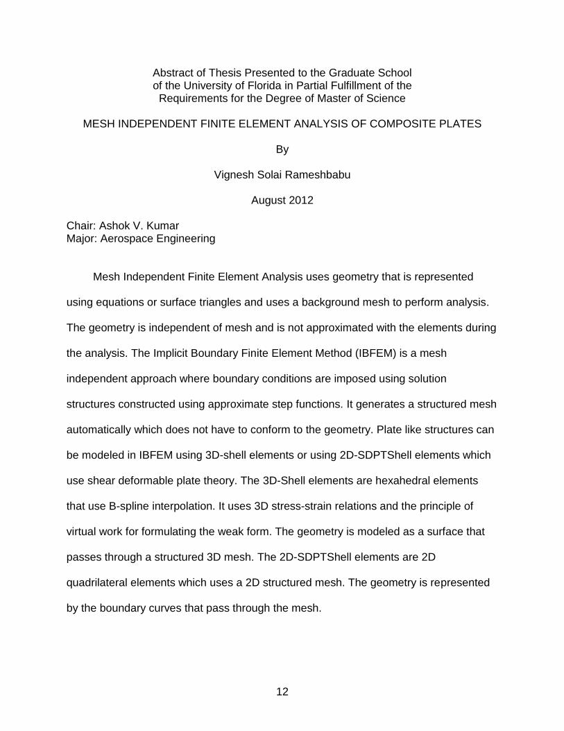
Mesh Independent Finite Element Analysis uses geometry that is represented
using equations or surface triangles and uses a background mesh to perform analysis.
The geometry is independent of mesh and is not approximated with the elements during
the analysis. The Implicit Boundary Finite Element Method (IBFEM) is a mesh
independent approach where boundary conditions are imposed using solution
structures constructed using approximate step functions. It generates a structured mesh
automatically which does not have to conform to the geometry. Plate like structures can
be modeled in IBFEM using 3D-shell elements or using 2D-SDPTShell elements which
use shear deformable plate theory. The 3D-Shell elements are hexahedral elements
that use B-spline interpolation. It uses 3D stress-strain relations and the principle of
virtual work for formulating the weak form. The geometry is modeled as a surface that
passes through a structured 3D mesh. The 2D-SDPTShell elements are 2D
quadrilateral elements which uses a 2D structured mesh. The geometry is represented
by the boundary curves that pass through the mesh.

13
In thesis, we extend these two approaches for modeling plates to include the
ability to model unidirectional composite laminates. The laminate is defined by the
number of layers, orientation, material properties and thickness of each lamina. Using
these, the effective properties of the laminate are usually computed as a relation
between force/moment resultants and strain/curvature. This can be directly used for the
2D-SDPTShell because it uses the weak form that is derived from the equations of the
Shear Deformable Plate Theory (SDPT). For the 3D-shell approach, a 3D stress-strain
relation is needed. This relation is determined from the effective properties of the
laminate including the relation between force resultants and strains, the coupling
between bending and in-plane forces, moment resultants and curvatures as well as
shears force resultants and shear strains. These two types of elements are developed
and compared using some standard and practical examples in different test cases and
using different boundary conditions. The results are compared with analytical solutions,
when available, or with commercial finite element analysis software. The convergence
rate of these two elements is compared. Finally, the advantages and disadvantages of
the two elements and future applications/extensions are discussed.
14
CHAPTER 1 INTRODUCTION
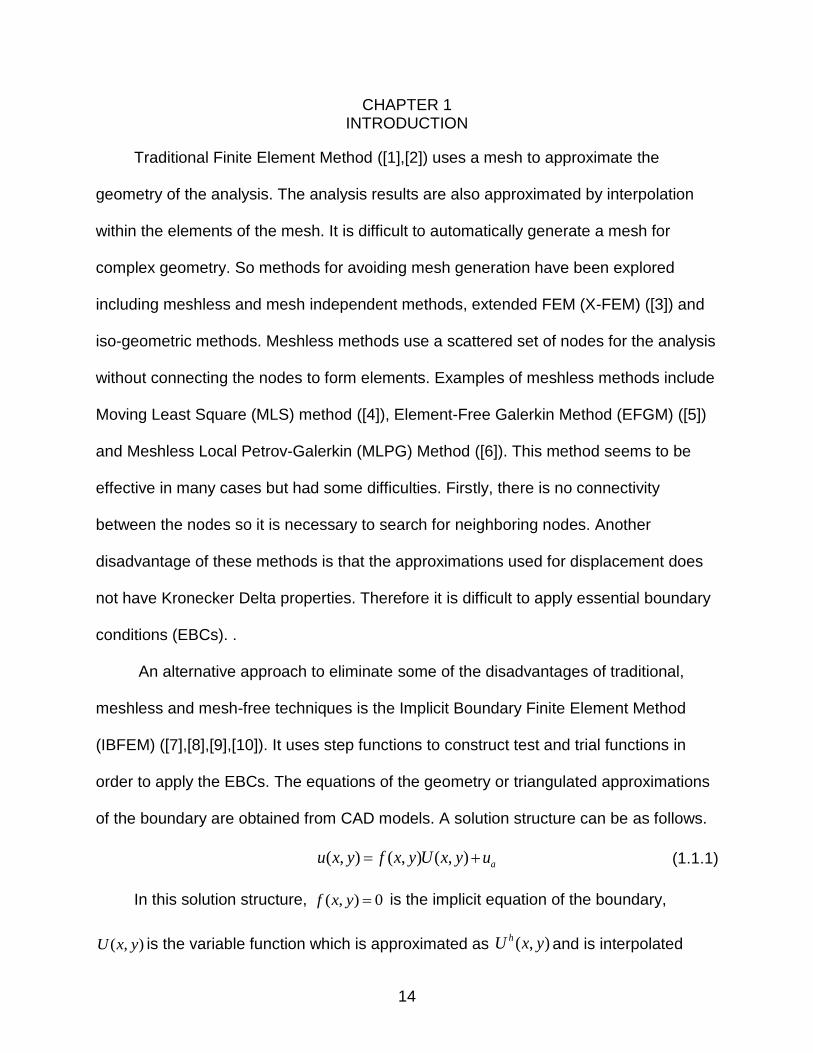
Traditional Finite Element Method ([1],[2]) uses a mesh to approximate the
geometry of the analysis. The analysis results are also approximated by interpolation
within the elements of the mesh. It is difficult to automatically generate a mesh for
complex geometry. So methods for avoiding mesh generation have been explored
including meshless and mesh independent methods, extended FEM (X-FEM) ([3]) and
iso-geometric methods. Meshless methods use a scattered set of nodes for the analysis
without connecting the nodes to form elements. Examples of meshless methods include
Moving Least Square (MLS) method ([4]), Element-Free Galerkin Method (EFGM) ([5])
and Meshless Local Petrov-Galerkin (MLPG) Method ([6]). This method seems to be
effective in many cases but had some difficulties. Firstly, there is no connectivity
between the nodes so it is necessary to search for neighboring nodes. Another
disadvantage of these methods is that the approximations used for displacement does
not have Kronecker Delta properties. Therefore it is difficult to apply essential boundary
conditions (EBCs). .
An alternative approach to eliminate some of the disadvantages of traditional,
meshless and mesh-free techniques is the Implicit Boundary Finite Element Method
(IBFEM) ([7],[8],[9],[10]). It uses step functions to construct test and trial functions in
order to apply the EBCs. The equations of the geometry or triangulated approximations
of the boundary are obtained from CAD models. A solution structure can be as follows.
( , ) ( , ) ( , ) au x y f x y U x y u (1.1.1)
In this solution structure, ( , ) 0f x y is the implicit equation of the boundary,
( , )U x y is the variable function which is approximated as ( , )hU x y and is interpolated
15
piecewise throughout the mesh and au is the prescribed value of the essential boundary
condition. In this method, a background mesh is generated around the geometry and
the integration is done by directly using the implicit equations of the geometry.
Therefore it is also known as Implicit Boundary Finite Element Method (IBFEM). The
accuracy is improved because the geometry equations are directly used and is not
approximated using elements. The main goal of this thesis is applying this method for
analyzing composite plates. Two different approaches for modeling plates were used
implement composite material properties. One uses 3D elements and cubic B-spline
approximation functions while the other uses Shear Deformable Plate theory and mixed
formulation approach.
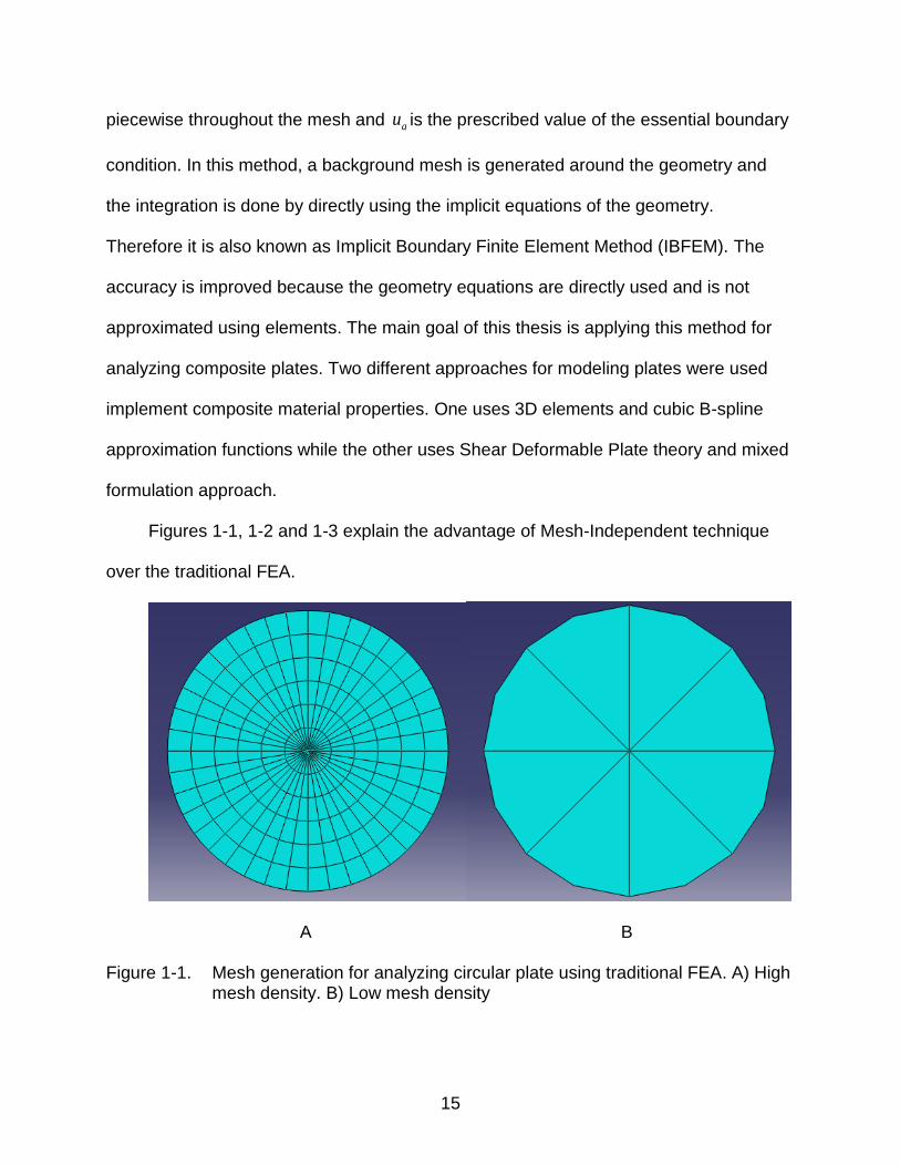
Figures 1-1, 1-2 and 1-3 explain the advantage of Mesh-Independent technique
over the traditional FEA.
A B
Figure 1-1. Mesh generation for analyzing circular plate using traditional FEA. A) High mesh density. B) Low mesh density

16
Figure 1-1 shows the mesh generated for an analysis of circular plate using
traditional FEA. From the figure, it is clear that the mesh generated is approximated for
the whole geometry and the mesh seems to be conforming when the mesh density is
high. But, when the mesh density is poor, the mesh does not conform to the geometry.
This problem can be overcome by implementing mesh-free technique since it does not
approximate the geometry by replacing it with meshes and it directly uses the equation
of the geometry. So, the mesh density does not affect the accuracy of the geometry.
A B
Figure 1-2. 3D mesh generation for analyzing circular plate using IBFEM. A) High mesh density. B) Low mesh density
Figure 1-2 clearly shows the 3D mesh generation for the analysis of circular plate
using IBFEM. As seen in the figure, the geometry is not replaced by the mesh but it
directly uses the equation of the geometry. Each element is 3D and the plate passes
through the elements.
To overcome some of the difficulties in the 3D element, a new element which uses
Shear Deformable Plate Theory is developed. Since, this element is exclusively
developed for composite plates; it is enough if only 2D meshes are generated. Hence

17
the grids generated for this analysis is 2D which is shown in figure 1-3. In this method,
the equations from the Shear Deformable Plate Theory (SDPT) are used for the
formulation of weak form. Hence, the in-plane stiffness [A], coupling stiffness [B] and
bending stiffness [D] of the laminate and is directly used in the formulation which
reduces the error percentage of the result.
A B
Figure 1-3. 2D mesh generation for analyzing circular plate using IBFEM. A) High mesh density. B) Low mesh density
Goals and Objectives
Goal
The main goal of this thesis is to develop composite plate elements which
implement the idea of mesh-independent Finite Element Method.
Objectives
Implement composite material properties for 3D shell elements to model flat
composite laminates where the geometry is modeled as a planar surface that is
imported from CAD software and mesh is a background structured mesh consisting of
uniform 3D cubic/cuboid elements.
18
Implement composite material properties for 2D Mindlin plate elements. This
method uses the equations of Shear Deformable Plate Theory (SDPT) directly for
formulation. Moreover, the stiffness matrix is defined from the in-plane stiffness,
coupling stiffness and bending stiffness matrix. The geometry is again a planar surface
and the mesh is a 2D background mesh with uniform square/rectangular elements.
Compare the performance of these two elements for modeling plates.
Perform convergence studies for some standard examples that have analytical
solutions and also perform convergence studies for some practical examples.
Compare results with commercial FEA software.
Outline
The remaining portion of the thesis is systematized as follows:
In Chapter 2, the introduction of composite materials, its types and its application
in engineering is explained. It also discloses the history of finite element analysis of
composite plates and the past work on composite FEA. This chapter also explains the
methods used for structural analysis of composite plates. It also gives the equation used
for structural analysis and determination of strength. Moreover, it also explains the two
major plate theories and its equations used in the Finite Element formulation.
In Chapter 3, explains the need for mesh-free finite element analysis and the past
work of researchers in this area. It also clarifies the concept of Implicit Boundary Finite
Element Method (IBFEM) and the use of step function in its formulation. It also explains
the calculation of stiffness matrix in this formulation.
In Chapter 4, the implementation of IBFEM for composite plates is explained. It
also explains the determination of equivalent stiffness of the composite laminate from

19
the material properties of the individual lamina which can be used in the formulation of
3D element. The constitutive model used in plate theory formulation is also explained.
In Chapter 5, various examples have been used to test the composite plates and
mixed formulation in IBFEM of composite plates. The first example explains it through
the 1-D analysis of composite beam. The second example proves the concept in 2-D
analysis in Composite Square Plate. The third example is a practical example which
proves the concept in the Composite Wing of a Micro-Air-Vehicle (MAV). It shows
clearly that IBFEM is effective in such cases as it is a good example of non-conforming
mesh type. The fourth example involves the analysis of a composite square plate with a
hole at the center. It also contains convergence plots for each example in various cases
such as different boundary conditions, various possible stacking sequences which
clearly shows that this method is the most cheap and efficient method for Finite-Element
Method of Composite Plates.
In Chapter 6, summary of the work and the conclusions drawn from the results are
provided. The advantages and disadvantages of the two approaches are explained and
the appropriate condition to use the two elements which is formulated from two different
methods is deduced. This chapter also clearly explains the research work which can be
done in the future in extension to the current research.

20
CHAPTER 2 ANALYSIS OF COMPOSITE MATERIALS
Overview
Composite materials, as per the definition, are obtained from the combination of
two or more distinct materials. They are designed to satisfy design criteria such that the
properties of the whole are better than the sum of the properties of each constituent
taken separately. It is different from isotropic materials as its property varies according
to the location and direction. As they give a very high strength to weight ratio, they are
also known as high-performance materials and are used in aerospace and automotive
applications. Some of the secondary advantages of composite materials are, they are
corrosion resistant, friction and wear resistant, vibration damping, fire resistant,
acoustical insulation, piezoelectric etc. There are various types of composites such as
particle-reinforced plastics (PRP), fiber-reinforced plastics (FRP), laminated plastics etc.
Among these, the most frequently used type of composites are FRPs and laminated
composites as the mechanical properties of the material can be calculated from the
location and the orientation of the fiber. The frequently used FRPs in engineering
applications are unidirectional composites as it gives an enhanced strength in a
particular direction which is aligned with the direction of loads acting on the component.
The design of components using these materials is different from those from
isotropic materials because, in this case, the material is made at the same time as the
component. As the material is fabricated according to the design specifications of the
component, designers/engineers should pay attention to the methods used to fabricate
the material which is a big factor which can affect the design of the component. Hence
there should be a better communication between the design and manufacturing to

21
ensure optimal result. Several methods are used for predicting and study the properties
of composites including analytical/classical methods, experimental methods and finite-
element methods. Analytical methods which include macro-mechanics and micro-
mechanics are the one which uses equilibrium, constitutive and compatibility equations
to derive the governing equations which in turn are solved to find the stresses and
displacements. Experimental methods are used to find the properties and strength of
the material by performing various tests in the Universal Testing Machine (UTM)
according to ASTM standards. Since these methods are limited to simple geometries,
finite-element method (FEM) [11],[12],[13],[14] is increasing being used by
designers/engineers to model and analyze composite structures. J.N. Reddy [15]
proposed a method to implement Shear Deformable Plate Theory (SDPT) in FEM.
Automatic mesh generation is difficult when the geometry is complex. Several
meshless and meshfree methods have been developed that try to avoid using a mesh
for the analysis. R.J. Razzaq, A. El-Zafrany [16] explained how to use reduced mesh for
the non-linear analysis of composite plates and shells. J. Sladek, V. Sladek and S.N.
Atluri [17] introduced Meshless Local Petrov-Galerkin Method (MLPG) in anisotropic
Elasticity. Similarly, J. Belinha and L.M.J.S. Dinis [18] came up with the idea of Element
Free Galerkin Method (EFGM) in analyzing composite laminates. The next stage of
development in the FEA research in composites leads to development of Higher order
Displacement model [19] and the introduction of Higher Order Shear and Normal
Deformable Plate Theory (HOSNDPT) and the Meshless Method with Radial Basis
Functions by J.R. Xiao, D.F. Gilhooley, R.C. Batra, J.W. Gillespie Jr., M.A. McCarthy

22
[19]. This chapter contains the derivation of the equations and the relations used for the
formulation in Shear deformable plate theory.
Stress-Strain Relations of a Composite Lamina
Composite materials are obtained by the combination of two or more materials at
macro scale and its behavior is describable by continuum mechanics. As it contains a
continuous phase called matrix and a discontinuous phase called fibers, its properties
are different at different point and direction.
Figure 2-1. Composite lamina
Figure 2-1 shows that the direction along the fiber is 1 and the direction
perpendicular to the fiber is 2. From the generalized Hooke’s Law, the general form of
Stress-Strain relation [21][22][23][24][25] is given by,
1 111 12 13 14 15 16
2 212 22 23 24 25 26
3 313 23 33 34 35 36
14 24 34 44 45 4623 23
15 25 35 45 55 5631 31
16 26 36 46 56 6612 12
Q Q Q Q Q Q
Q Q Q Q Q Q
Q Q Q Q Q Q
Q Q Q Q Q Q
Q Q Q Q Q Q
Q Q Q Q Q Q
(2.2.1)
The above equation refers to the Stress-Strain relation of anisotropic materials
(or) otherwise known as triclinic materials (i.e.) the three axes of the material are
1
2
Fiber cross section
23
oblique to one another. Because it is assumed to be hyper elastic, the [C] matrix
becomes symmetric and hence Cij = Cji. Hence we have 21 stiffness co-effecients.
If there is only one pair of symmetry of the material property, the Stress-Strain
relation becomes,
1 111 12 13 16
2 212 22 23 26
3 313 23 33 36
44 4523 23
45 5531 31
16 26 36 6612 12
0 0
0 0
0 0
0 0 0 0
0 0 0 0
0 0
Q Q Q Q
Q Q Q Q
Q Q Q Q
Q Q
Q Q
Q Q Q Q
(2.2.2)
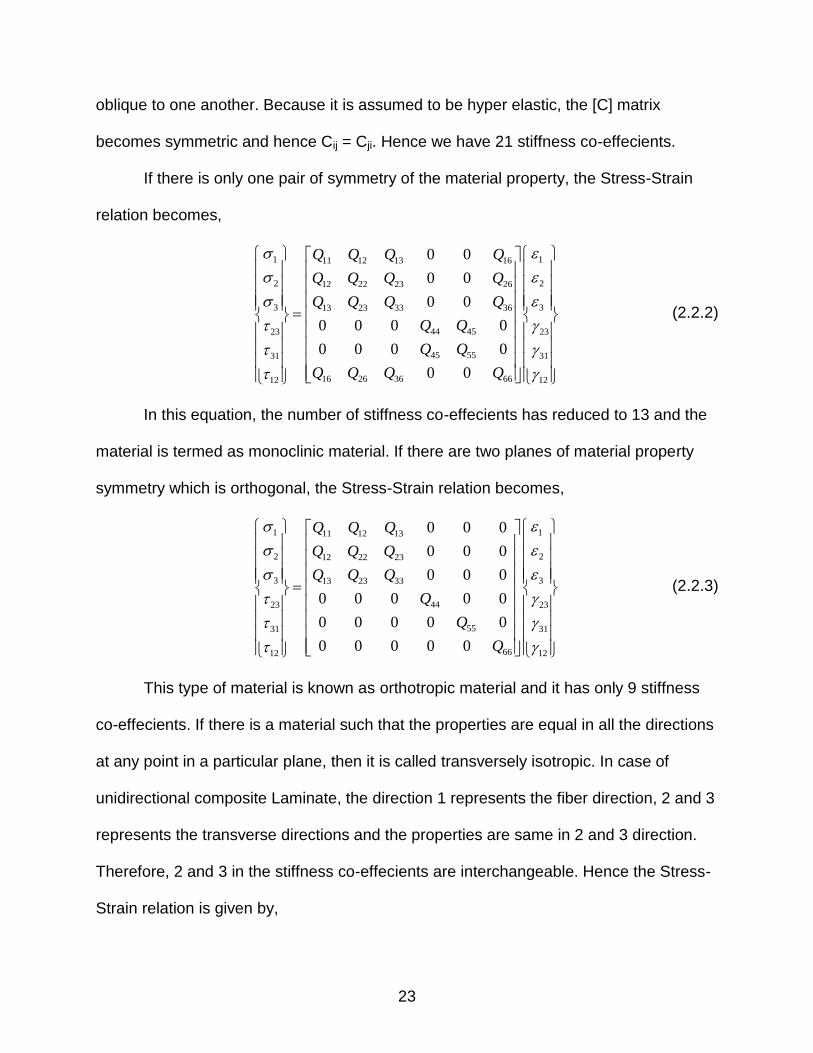
In this equation, the number of stiffness co-effecients has reduced to 13 and the
material is termed as monoclinic material. If there are two planes of material property
symmetry which is orthogonal, the Stress-Strain relation becomes,
1 111 12 13
2 212 22 23
3 313 23 33
4423 23
5531 31
6612 12
0 0 0
0 0 0
0 0 0
0 0 0 0 0
0 0 0 0 0
0 0 0 0 0
Q Q Q
Q Q Q
Q Q Q
Q
Q
Q
(2.2.3)
This type of material is known as orthotropic material and it has only 9 stiffness
co-effecients. If there is a material such that the properties are equal in all the directions
at any point in a particular plane, then it is called transversely isotropic. In case of
unidirectional composite Laminate, the direction 1 represents the fiber direction, 2 and 3
represents the transverse directions and the properties are same in 2 and 3 direction.
Therefore, 2 and 3 in the stiffness co-effecients are interchangeable. Hence the Stress-
Strain relation is given by,
24
1 111 12 13
2 212 22 23
3 313 23 33
22 2323 23
6631 31
6612 12
0 0 0
0 0 0
0 0 0
0 0 0 ( ) / 2 0 0
0 0 0 0 0
0 0 0 0 0
Q Q Q
Q Q Q
Q Q Q
Q Q
Q
Q
(2.2.4)
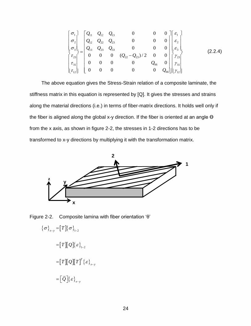
The above equation gives the Stress-Strain relation of a composite laminate, the
stiffness matrix in this equation is represented by [Q]. It gives the stresses and strains
along the material directions (i.e.) in terms of fiber-matrix directions. It holds well only if
the fiber is aligned along the global x-y direction. If the fiber is oriented at an angle Ɵ
from the x axis, as shown in figure 2-2, the stresses in 1-2 directions has to be
transformed to x-y directions by multiplying it with the transformation matrix.
Figure 2-2. Composite lamina with fiber orientation ‘θ’
1 2
1 2
x y
T
x y
x y
T
T Q
T Q T
Q
y
x
z
1
2
25
x y x yQ
σ ε (2.2.5)
Where, [ ̅] = [T] [Q] [T] T and the Transformation matrix is given by,
2 2
2 2
2 2
0 0 0 2
0 0 0 2
0 0 1 0 0 0
0 0 0 0
0 0 0 0
0 0 0
m n mn
n m mn
Tm n
n m
mn mn m n
(2.2.6)
Where m = cos θ and n = sin θ. When the fibers are oriented along the direction
which is at an angle Ɵ to the x axis, the Stress-Strain relation in x-y direction is given
by,
11 12 13 16
12 22 23 26
13 23 33 36
44 45
45 55
16 26 36 66
0 0
0 0
0 0
0 0 0 0
0 0 0 0
0 0
xx xx
yy yy
zz zz
yz yz
xz xz
xy xy
Q Q Q Q
Q Q Q Q
Q Q Q Q
Q Q
Q Q
Q Q Q Q
(2.2.7)
Where,
4 2 2 4
11 11 12 66 22
4 2 2 4
12 11 22 66 1212
2 2
13 2313
3 3
11 12 66 66 12 2216
4 2 2 4
22 12 66 1122
2 2
23 1323
2 2
4
2 2
2 2
Q Q m Q Q m n Q n
Q Q m Q Q Q m n Q n
Q Q m Q n
Q Q Q Q m n Q Q Q mn
Q Q m Q Q m n Q n
Q Q m Q n
26
3 3
12 22 66 11 12 6626
3333
13 2336
2 2 4 4
11 22 12 66 6666
2 2
44 5544
55 4445
2 2
55 4455
2 2
( 2 2 ) ( )
Q Q Q Q m n Q Q Q mn
Q Q
Q Q Q mn
Q Q Q Q Q m n Q m n
Q Q m Q n
Q Q Q mn
Q Q m Q n
For Plane stress condition, the above stress – strain relation can be written as,
11 12 16
12 22 26
16 26 66
xx xx
yy yy
xy xy
Q Q Q
Q Q Q
Q Q Q
(2.2.8)
Stress-Strain Relations of a Composite Laminate
Classical Lamination Plate Theory (CLPT)
In aerospace and automotive applications, unidirectional fiber composites are
widely used. The properties of unidirectional composites are close to transversely
isotropic materials. There are several other types of composites such as woven and
braided composites whose properties are close to orthotropic materials. These
unidirectional composites are using mats which are laminated layer by layer to form
plates. Here we introduce the classical lamination plate theory (CLPT) which makes the
following assumptions.
Stiffness and Stresses are averaged through the thickness.
x-y plane is the middle plane of the plate and z-axis is the thickness direction.
27
The thickness of the plate is so small when compared to the lateral dimensions of
the plate.
The displacements u, v and w are very small when compared to the plate
thickness. This theory is known as Small Displacement Theory.
The in-plane strains are very small when compared to unity.
The transverse shear strains are negligible. (i.e.) 0; 0;xz yz .The thickness
change is also very small and so the transverse normal strain can be neglected. (i.e.)
0z .
The transverse normal and shear stresses are negligibly small when compared to
in-plane stresses.
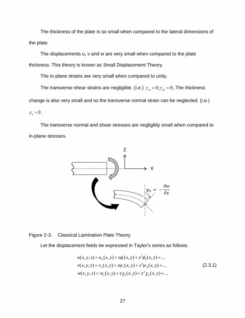
Figure 2-3. Classical Lamination Plate Theory
Let the displacement fields be expressed in Taylor's series as follows.
2
1 2
2
1 2
2
1 2
( , , ) ( , ) ( , ) ( , ) ...
( , , ) ( , ) ( , ) ( , ) ...
( , , ) ( , ) ( , ) ( , ) ...
o
o
o
u x y z u x y z x y z x y
v x y z v x y z x y z x y
w x y z w x y z x y z x y
(2.3.1)
𝜑𝑥 = −𝜕𝑤
𝜕𝑥
X
Z

28
Eliminating the higher order terms and assuming the transverse displacement
independent of z-coordinate, eqns (2.3.1) becomes,
1
1
( , , ) ( , ) ( , )
( , , ) ( , ) ( , )
( , , ) ( , )
o
o
o
u x y z u x y z x y
v x y z v x y z x y
w x y z w x y
(2.3.2)
From the Small-Strain Theory, the transverse shear strains can be derived as:
xz
yz
u w
z x
v w
z y
(2.3.3)
Substituting eqns (2.3.2) in eqns (2.3.3),
1
1
( , )
( , )
xz
yz
wx y
x
wx y
y
(2.3.4)
In CLPT, as the transverse shear strains are assumed to be negligible, (i.e.)
0; 0;xz yz eqns. (2.3.4) becomes,
1
1
w
x
w
y
(2.3.5)
Substituting eqns. (2.3.5) in eqns. (2.3.2), we get,
( , , ) ( , )
( , , ) ( , )
( , , ) ( , )
o
o
o
wu x y z u x y z
x
wv x y z v x y z
y
w x y z w x y
(2.3.6)
From the above equation, the in-plane strains can be derived as,

29
0
0
0
x x x
y y y
xy xy xy
z
z
z
(2.3.7)
Where ,xo yo and 0xy are the mid-plane strains and , ,x y xy are the curvatures
which can be defined as follows:
0 0 0 00 0 0
2 2 2
2 2
; ;
; ; 2
x y xy
x y xy
u v u v
x y y x
w w w
x y x y
(2.3.8)
Eqn. (2.3.7) can be written in Matrix form as follows:
0
0
0
x x x
y y y
xy xy xy
z
(2.3.9)
z 0 (2.3.10)
The three dimensional equations of motion for a body considering the large
deformations are,
2
2
ki i ikj i
k k j
u uB
x x x t
From these equations of equilibrium, without considering body forces and large
deformations and neglecting the product of transverse stresses and in-plane strains in
the non-Linear terms which are small, we get,
2
2
2
2
2
2
yxx zx
xy y zy
xz x xy yz xy y z xz yz
u
x y y t
v
x y y t
w w w w w w w
x x y y x y z x y t
(2.3.11)
30
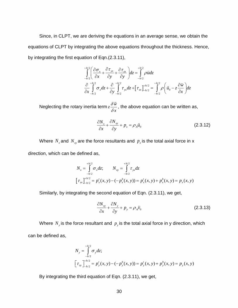
Since, in CLPT, we are deriving the equations in an average sense, we obtain the
equations of CLPT by integrating the above equations throughout the thickness. Hence,
by integrating the first equation of Eqn.(2.3.11),
/2 /2
/2 /2
/2 /2 /2/2
0/2
/2 /2 /2
h hyxx zx
h h
h h hh
x yx zx h
h h h
dz udzx y y
wdz dz u z dz
x y x
Neglecting the rotary inertia termw
zx
, the above equation can be written as,
0
xyxx A
NNp u
x y
(2.3.12)
Where xN and xyN are the force resultants and xp is the total axial force in x
direction, which can be defined as,
/2 /2
/2 /2
/2
/2
;
( , ) ( ( , )) ( , ) ( , ) ( , )
h h
x x xy yx
h h
h t b t b
zx x x x x xh
N dz N dz
p x y p x y p x y p x y p x y
Similarly, by integrating the second equation of Eqn. (2.3.11), we get,
0
xy y
y A
N Np v
x y
(2.3.13)
Where yN is the force resultant and yp is the total axial force in y direction, which
can be defined as,
/2
/2
/2
/2
;
( , ) ( ( , )) ( , ) ( , ) ( , )
h
y y
h
ht b t b
zy y y y y yh
N dz
p x y p x y p x y p x y p x y
By integrating the third equation of Eqn. (2.3.11), we get,
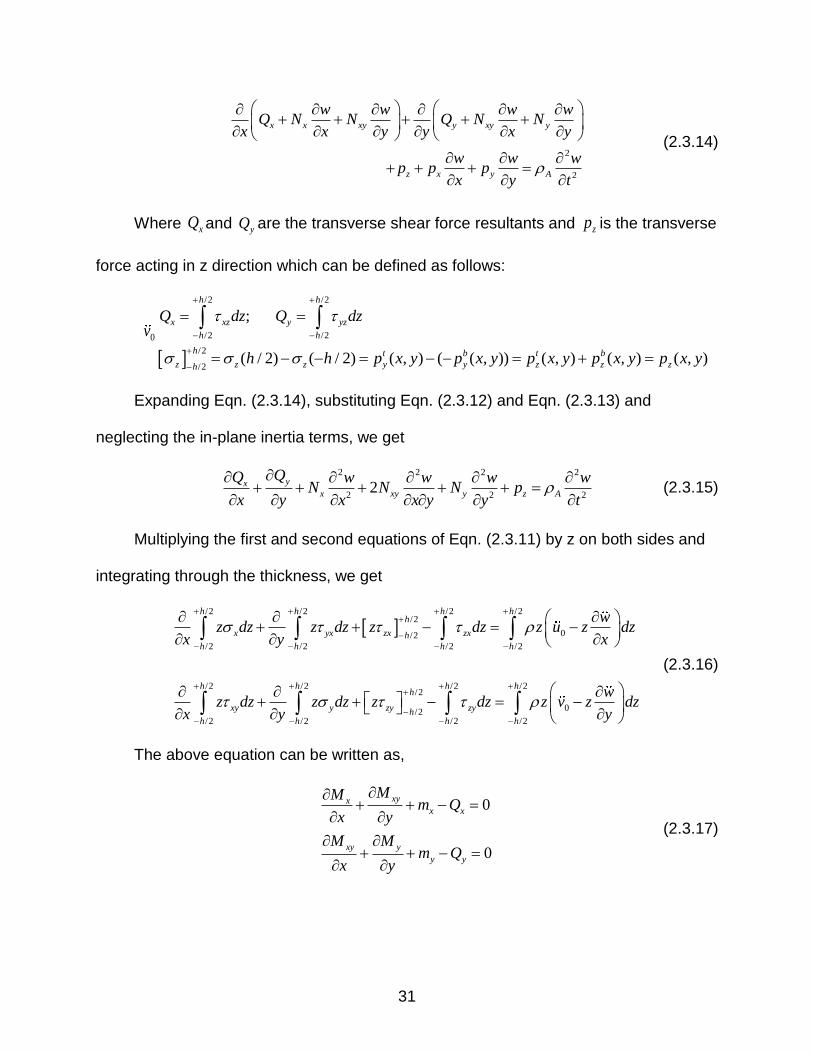
31
2
2
x x xy y xy y
z x y A
w w w wQ N N Q N N
x x y y x y
w w wp p p
x y t
(2.3.14)
Where xQ and yQ are the transverse shear force resultants and zp is the transverse
force acting in z direction which can be defined as follows:
0v
/2 /2
/2 /2
/2
/2
;
( / 2) ( / 2) ( , ) ( ( , )) ( , ) ( , ) ( , )
h h
x xz y yz
h h
h t b t b
z z z y y z z zh
Q dz Q dz
h h p x y p x y p x y p x y p x y
Expanding Eqn. (2.3.14), substituting Eqn. (2.3.12) and Eqn. (2.3.13) and
neglecting the in-plane inertia terms, we get
2 2 2 2
2 2 22
yxx xy y z A
QQ w w w wN N N p
x y x x y y t
(2.3.15)
Multiplying the first and second equations of Eqn. (2.3.11) by z on both sides and
integrating through the thickness, we get
/2 /2 /2 /2
/2
0/2
/2 /2 /2 /2
/2 /2 /2 /2/2
0/2/2 /2 /2 /2
h h h hh
x yx zx zxh
h h h h
h h h hh
xy y zy zyhh h h h
wz dz z dz z dz z u z dz
x y x
wz dz z dz z dz z v z dz
x y y
(2.3.16)
The above equation can be written as,
0
0
xyxx x
xy y
y y
MMm Q
x y
M Mm Q
x y
(2.3.17)
32
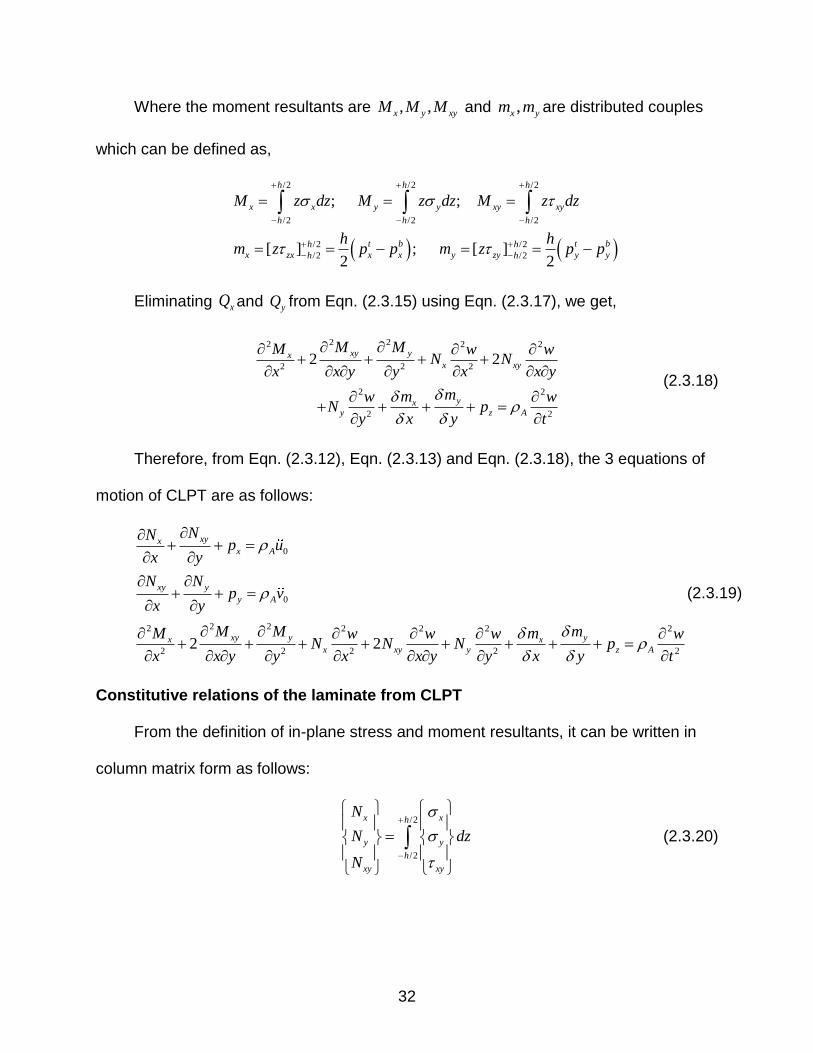
Where the moment resultants are , ,x y xyM M M and ,x ym m are distributed couples
which can be defined as,
/2 /2 /2
/2 /2 /2
/2 /2
/2 /2
; ;
[ ] ; [ ]2 2
h h h
x x y y xy xy
h h h
t b t bh h
x zx x x y zy y yh h
M z dz M z dz M z dz
h hm z p p m z p p
Eliminating xQ and yQ from Eqn. (2.3.15) using Eqn. (2.3.17), we get,
2 22 2 2
2 2 2
2 2
2 2
2 2xy yx
x xy
yxy z A
M MM w wN N
x x y y x x y
mmw wN p
y x y t
(2.3.18)
Therefore, from Eqn. (2.3.12), Eqn. (2.3.13) and Eqn. (2.3.18), the 3 equations of
motion of CLPT are as follows:
0
0
2 22 2 2 2 2
2 2 2 2 22 2
xyxx A
xy y
y A
xy y yx xx xy y z A
NNp u
x y
N Np v
x y
M M mM mw w w wN N N p
x x y y x x y y x y t
(2.3.19)
Constitutive relations of the laminate from CLPT
From the definition of in-plane stress and moment resultants, it can be written in
column matrix form as follows:
/2
/2
x xh
y y
h
xy xy
N
N dz
N
(2.3.20)

33
/2
/2
x xh
y y
h
xy xy
M
M zdz
M
(2.3.21)
Substituting Eqn. (2.2.8) in Eqn (2.3.20), we get
11 12 16/2
12 22 26
/2
16 26 66
11 12 16/2
12 22 26
/2
16 26 66
x xxh
y yy
h
xy xy
x xxh
y yy
h
xy xy
N Q Q Q
N Q Q Q dz
Q Q QN
M Q Q Q
M Q Q Q zdz
Q Q QM
(2.3.22)
Substituting Eqn. (2.3.7) in Eqn (2.3.21),
011 12 16/2
12 22 26 0
/2
16 26 66 0
/2
/2
x x xh
y y y
h
xy xy xy
h
h
N Q Q Q
N Q Q Q z dz
Q Q QN
z dz
0N Q
(2.3.23)
011 12 16/2
12 22 26 0
/2
16 26 66 0
/2
2
/2
x x xh
y y y
h
xy xy xy
h
h
M Q Q Q
M Q Q Q z zdz
Q Q QM
z z dz
0 M Q
(2.3.24)
The above equation can be further simplified as,
/2 /2
/2 /2
h h
h h
dz z dz
0
0
N
N
Q Q
A B
(2.3.25)
34
/2 /2
2
/2 /2
h h
h h
z dz z dz
0
0
M Q Q
M B D
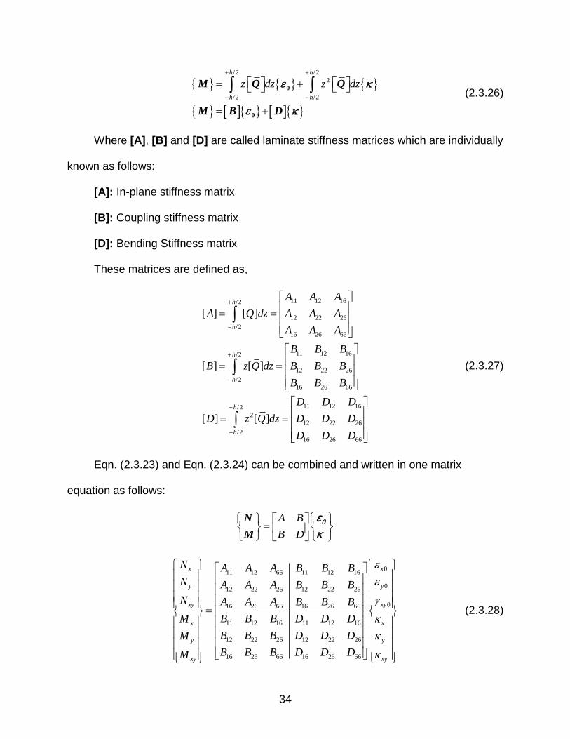
(2.3.26)
Where [A], [B] and [D] are called laminate stiffness matrices which are individually
known as follows:
[A]: In-plane stiffness matrix
[B]: Coupling stiffness matrix
[D]: Bending Stiffness matrix
These matrices are defined as,
11 12 16/2
12 22 26
/2
16 26 66
11 12 16/2
12 22 26
/2
16 26 66
11 12 16/2
2
12 22 26
/2
16 26 66
[ ] [ ]
[ ] [ ]
[ ] [ ]
h
h
h
h
h
h
A A A
A Q dz A A A
A A A
B B B
B z Q dz B B B
B B B
D D D
D z Q dz D D D
D D D
(2.3.27)
Eqn. (2.3.23) and Eqn. (2.3.24) can be combined and written in one matrix
equation as follows:
A B
B D
N
M
0ε
κ
011 12 66 11 12 16
012 22 26 12 22 26
016 26 66 16 26 66
11 12 16 11 12 16
12 22 26 12 22 26
16 26 66 16 26 66
x x
y y
xy xy
x x
y y
xy xy
N A A A B B B
N A A A B B B
N A A A B B B
B B B D D DM
B B B D D DM
B B B D D DM
(2.3.28)

35
Shear Deformable Plate Theory (SDPT)
This theory explains that one of the assumptions of CLPT that says the plane
sections normal to the mid-plane of the plate remain plane and normal after the plate
deforms is valid only in case of thin plates. This further explains that the transverse
shear strains xz and yz does not vanish and remain constant throughout the thickness
of the plate (i.e.), the plane sections normal to the mid-section remain plane but not
necessarily remain normal to the mid-surface after deformation.
Figure 2-4. Shear Deformable Plate Theory
The displacement fields can be expressed as,
( , , ) ( , ) ( , )
( , , ) ( , ) ( , )
( , , ) ( , )
o x
o y
o
u x y z u x y z x y
v x y z v x y z x y
w x y z w x y
(2.4.1)
Where x and y are rotations of the cross section about y axis and –x axis
respectively. The in-plane strains can be derived as,
−𝜕𝑤
𝜕𝑥
X
Z
Φx

36
0
0
0
x x x
y y y
xy xy xy
z
z
z
(2.4.2)
Where the mid-plane strains and curvatures are defined as,
0 0 0 00 0 0; ;
; ;
x y xy
y yx xx y xy
u v u v
x y y x
x x y x
(2.4.3)
Similarly, the equations of SDPT can be derived from the equilibrium equations
which are as follows:
0
0
2
2
0
0
xyxx A x
xy y
y A y
yxz A
xyxx x x
xy y
y y y
NNp u H
x y
N Np v H
x y
QQ wp
x y t
MMm Q Hu I
x y
M Mm Q Hu I
x y
(2.4.4)
Where,
/2
/2
/2
2
/2
h
h
h
h
H zdz
I z dz
37
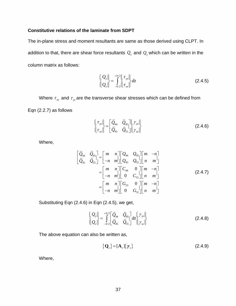
Constitutive relations of the laminate from SDPT
The in-plane stress and moment resultants are same as those derived using CLPT. In
addition to that, there are shear force resultants xQ and yQ which can be written in the
column matrix as follows:
/2
/2
hy yz
x h xz
Qdz
Q
(2.4.5)
Where xz and yz are the transverse shear stresses which can be defined from
Eqn (2.2.7) as follows
44 45
45 55
yz yz
xz xz
Q Q
Q Q
(2.4.6)
Where,
44 4544 45
45 5545 55
44
55
23
31
0
0
0
0
Q Qm n m nQ Q
Q Qn m n mQ Q
Cm n m n
Cn m n m
Gm n m n
Gn m n m
(2.4.7)
Substituting Eqn (2.4.6) in Eqn (2.4.5), we get,
/2
44 45
45 55/2
hy yz
x h xz
Q Q Qdz
Q QQ
(2.4.8)
The above equation can also be written as,
[ ]s s sQ A (2.4.9)
Where,

38
/2
44 45
45 55/2
44 45
45 55
[ ]
h
s
h
Q Qdz
Q Q
A A
A A
A
Eqn (2.3.23), Eqn. (2.3.24) and Eqn. (2.4.9) can be combined and written in the
form of one matrix equation to get the constitutive relation of the laminate which is as
follows:
s
N A B 0
M B D 0
0 0 A
sQ
0
s
ε
γ
(2.4.10)
The equation above, can be further written as,
11 12 16 11 12 16
12 22 23 12 22 26
16 26 66 16 26 66
11 12 16 11 12 16
12 22 23 12 22 23
16 26 66 16 26 66
44 45
45 55
0 0
0 0
0 0
0 0
0 0
0 0
0 0 0 0 0 0
0 0 0 0 0 0
x
y
xy
x
y
xy
y
x
N A A A B B BN A A A B B B
N A A A B B B
M B B B D D D
M B B B D D D
B B B D D DM
A AQ
A AQ
0
0
0
x
y
xy
x
y
xy
yz
xz
(2.4.11)
Eqn (2.4.11) gives the constitutive relation of the laminate using SDPT.

39
CHAPTER 3 MESH INDEPENDENT FINITE ELEMENT METHOD
Introduction
The most successful methods which are used to solve structural, thermal and fluid
flow problems are Finite Difference Method (FDM), Finite Element Method (FEM) and
Spectral Method. For structural analysis FEM is the most popular numerical method
because it can be used for arbitrary geometry as long as a mesh can be generated for
the analysis. Figure 3-1(a) shows the approximation of the whole geometry into a finite
element mesh. Automatic mesh generation is difficult for 3D problems. To avoid such
difficulties, a number of meshless or mesh-free analysis techniques have been
proposed in the past two decades. Belytschko.T, Y. Krongauz, D. Organ, M. Fleming, P.
Krysl [26] introduced meshless method and explained its implementation. J.J.
Monaghan [27] explained how mesh-free methods can be used to solve astrophysical
problems. This approach uses a scattered set of nodes all over the system for analysis
(figure 3-1(b)). One of the most widely used basis functions for scattered meshless
methods is Moving Least square (MLS) approximation which was clearly explained by
P.Lancaster and K.Salkauskas [4]. Followed by MLS, several other techniques such as
Element-Free Galerkin Method (EFGM) [5], Meshless local Petrov-Galerkin Method
(MLPG) [6] were consecutively developed. One of the main features of meshless
methods is, there is no connectivity between the nodes. An alternate approach to the
mesh-free method is using structured, non-conforming mesh, in which the geometry is
represented using implicit equations and therefore is independent of the mesh. Figure
3-1(c) shows the generation of non-conforming uniform, structured mesh.
40
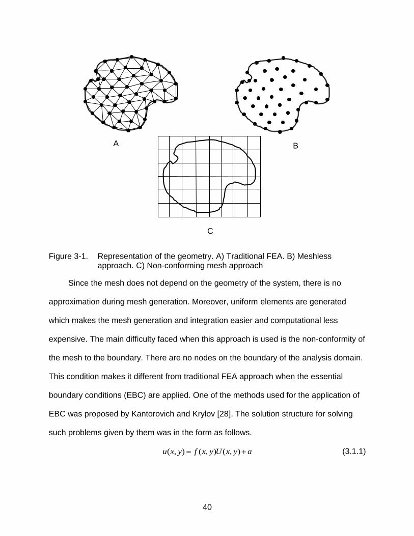
Figure 3-1. Representation of the geometry. A) Traditional FEA. B) Meshless approach. C) Non-conforming mesh approach
Since the mesh does not depend on the geometry of the system, there is no
approximation during mesh generation. Moreover, uniform elements are generated
which makes the mesh generation and integration easier and computational less
expensive. The main difficulty faced when this approach is used is the non-conformity of
the mesh to the boundary. There are no nodes on the boundary of the analysis domain.
This condition makes it different from traditional FEA approach when the essential
boundary conditions (EBC) are applied. One of the methods used for the application of
EBC was proposed by Kantorovich and Krylov [28]. The solution structure for solving
such problems given by them was in the form as follows.
( , ) ( , ) ( , )u x y f x y U x y a (3.1.1)
A B
C

41
In the above equation (Eqn. (3.1.1)), ( , )f x y is the equation of the boundary of the
domain and a is the essential boundary condition. The variable part of the solution
structure is the function ( , )U x y which is approximated as ( , )hU x y which is piecewise
interpolated over the grid. Several other techniques such as R-function technique were
developed by Shapiro and Tsukanov [29] and it was extended to non-linear vibrations of
thin plates by Lidia Kurpa, Galina Pilgun and Eduard Ventsel [30]. C. Daux, N. Moës, J.
Dolbow, N. Sukumar and T. Belytschko [3] proposed a similar method known as X-FEM
which is based on structured, uniform mesh and IBM. They introduced it to find the
stress distribution in crack tips and it was further extended to 2-D and 3-D crack
modeling.
Another approach used to solve such difficulties in boundary value problems is the
Implicit Boundary FEM (IBFEM) proposed by Kumar A.V.[7][8][9][10]. As discussed in
chapter – 1, this method constructs a solution structure for the displacement and virtual
displacement field using approximate step functions of the boundaries.
Figure 3-2 shows a shell subjected to gravity pressure. The structural analysis is
performed and the displacement contour is obtained from Abaqus which follows
traditional finite element method and IBFEM which uses uniform non conformal mesh.
The figure clearly shows the type of mesh used in traditional FEA and IBFEM. In
traditional FEA, the geometry is replaced by the meshes. But, in IBFEM, the geometry is
immersed in the structured mesh. For shell like structures IBFEM uses B-spline basis
functions which are C2 continuous (i.e.) the functions used are curvature continuous,
whereas the Lagrange interpolation functions are C0 continuous (i.e.) their magnitudes
are continuous.

42
A B
Figure 3-2. Representation of a shell. A) Traditional FEA. B) IBFEM
This thesis involves development of two types of elements for analyzing composite
plates and a comparative study of these two elements is done. One element named 3D-
Shell uses B-spline interpolation functions with 3D non conformal structured grid. As
shown in figure3-2(b), the geometry is surrounded by 3D mesh which is uniform
throughout the domain. The basis function used in this element is cubic in nature and
hence it is c2 continuous (i.e.) it is tangent and curvature continuous. Another element
named 2D-SDPTShell consists of 2D element with a two-dimensional background
mesh. The geometry is surrounded by 2D mesh and is non-conformal in nature. As the
analysis involves flat composite plates, the mesh generated is 2D. It involves
interpolation functions that are not tangent continuous which involve Mindlin Plate
formulation as it uses the equations from Shear Deformable Plate Theory (SDPT). The
formulation of these two elements is explained as follows.
Formulation of 3D Element (3D-Shell)
The implicit boundary finite element method uses implicit equation in its solution
structure which is as follows.

43
{ } [ ]{ } { }H g au u u (3.1.2)
Where,
{ }u - Trail function
{ }gu - Piecewise approximation of the element of the structured grid
derived from the implicit equation of the boundary.
{ }au - Boundary value function which contains the essential boundary
condition
[ ]H - Diagonal matrix whose components are the step functions.
In this research, as the discussion is about composite plates and shells, the
formulation is similar to isotropic plates and shells. First, the plate is integrated over the
area of the mid-section and then the integration through the thickness is performed.
The volume of the shell can be represented as
ˆ( , , ) ( , )2
hX x n (3.1.3)
Where
( , )x - Parametric equation of the surface representing the mid-plane.
h - Total thickness of the shell
n̂ - Unit normal to the surface
[ 1,1]
The volume of the shell can also be represented in terms of unit normal and bi-
normal as
ˆˆ( , , ) ( )i i iX n b (3.1.4)
Where,

44
( )i - Parametric equation of the ith boundary
ˆin - Unit normal to the surface at the respective boundary
ˆib - Unit bi-normal to the surface at the respective boundary which is
the cross product of the unit normal and unit tangent of the boundary,
where the unit tangent is the first derivative of the equation of the
boundary for which the tangent is to be determined.
Figure 3-3. Representation of volume of a shell
Clamped boundary condition
Figure 3-4. Clamped boundary condition of a plate/shell
45
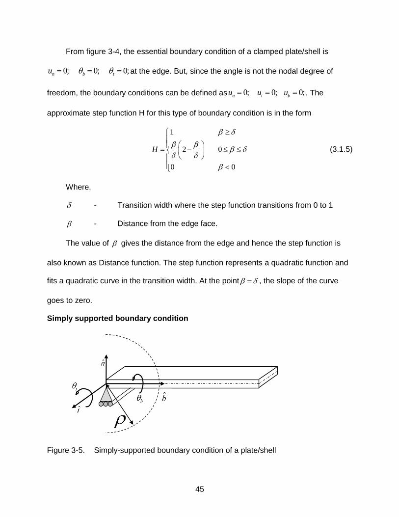
From figure 3-4, the essential boundary condition of a clamped plate/shell is
0; 0; 0;n b tu at the edge. But, since the angle is not the nodal degree of
freedom, the boundary conditions can be defined as 0; 0; 0;n t bu u u . The
approximate step function H for this type of boundary condition is in the form
1
2 0
0 0
H
(3.1.5)
Where,
- Transition width where the step function transitions from 0 to 1
- Distance from the edge face.
The value of gives the distance from the edge and hence the step function is
also known as Distance function. The step function represents a quadratic function and
fits a quadratic curve in the transition width. At the point , the slope of the curve
goes to zero.
Simply supported boundary condition
Figure 3-5. Simply-supported boundary condition of a plate/shell

46
From the figure 3-5, the essential boundary condition of a clamped plate/shell is
0;nu at the edge. Hence the approximate step function is defined as,
1
2 0
0 0
H
(3.1.6)
Where,
- Radial distance from the edge which is given by 2 2
Symmetric boundary condition
When a symmetric structure is to be analyzed; only a part of it is modeled to
reduce the model size (total number of elements) and therefore the computational time
is greatly reduced. The essential boundary condition of this type of boundary condition
is 0; ( . .) 0t bi e u . Hence the step function of this boundary condition is same as Eqn.
3.1.6 but can be applied only for bu .
B-Spline Basis Functions
Basis functions are used to map between the local and the global co-ordinate
system. In traditional FEA, Lagrange interpolation functions are used as basis functions
which are c0 continuous. But in the IBFEM, B-spline basis functions are used which
gives a higher degree of up to c2 continuity. Since the structured, uniform grids are
used, uniform B-spline basis functions are used in this case.
There are 2 types of basis functions used in two different types of elements. They
are quadratic B-spline basis functions which are C1 continuous and cubic B-spline basis
functions [31] which are C2 continuous. The concept of recursion (i.e.) calling a function

47
or a polynomial again and again is used to construct this basis function. Here is an
example for 1-D cubic B-spline basis function.
Figure 3-6. 1-D cubic B-spline approximation
In the figure, it is clear that the element E1 goes from node 2 to 3. The element is
actually controlled by four nodes starting from 1 through 4. Hence these nodes are also
known as support nodes. The approximated values such as displacement at a specific
node are not equal to the nodal value.
The cubic B-spline basis functions can be represented as follows.
2 3
1
2 3
2
2 3
3
2 3
4
1(1 3 3 );
48
1(23 15 3 3 );
48
1(23 15 3 3 );
48
1(1 3 3 );
48
N r r r
N r r r
N r r r
N r r r
(3.1.7)
Since the functions are cubic in nature (i.e.) the order of the function is 3, there are
4 basis functions and 4 support nodes, in which 2 nodes lie outside the element.
1 2 3 4 E1
Nodal Values
Approximated Function
Nodes
Elements

48
The basis functions of 2-D cubic B-spline basis functions can be constructed from
the product of two 1-D cubic basis functions.
2
4( 1)
3
16( 1) 4( 1)
( , ) ( ) ( ) 1,...,3; 1,...,3
( , , ) ( ) ( ) ( ) 1,...,3; 1,...,3; 1,...,3
D
j i i j
D
k j i i j k
N r s N r N s i j
N r s t N r N s N t i j k
(3.1.8)
Figure 3-7. 2-D cubic B-spline elements
From figure 3-7, it is shown that each 2-D element is supported by 16 support
nodes and 16 basis functions. Hence, a 2-D cubic basis element has 16 basis functions
and a 3-D cubic basis element has 64 functions.
Stiffness Matrix
In the 3D element approach, the weak form used is the 3D Principle of Virtual
Work, which can be expressed as follows,
{ } { } { } { } { } { } { } { }
t
T T T T
bd u T d u F d u f d
(3.1.9)
Where
{ } - Virtual Strain
{ } - Cauchy Stress tensor
t - Edges on which the traction is applied
{ }T - Traction vector
13 14 15 16
9 10 11 12
1 2 3 4
5 6 7 8

49
{ }u - Virtual displacement
{ }bF - Body force
{ }f - Pressure load per unit area
For plates and shells, the weak form (Eqn. 3.1.12) can be written as
1
0
1 1
1 1
1
1
{ } { } { } { }2 2
{ } { } { } { }2
t
A t
A
T T tA
T T
b A
dh hd d u T d d
d
hu F d d u f d
(3.1.10)
The strains and stresses can be broke down into homogenous and boundary
value part as,
( )
h a
h a h aC C
(3.1.11)
Substituting Eqn. (3.1.14) in Eqn. (3.1.13), we get,
1
0
1 1 1
1 1 1
1
1
{ } { } { } { } { } { }2 2 2
{ } { } { } { }2
t
t
T h T a T t
T T
b
dh h hC d d d d u T d d
d
hu F d d u f d
(3.1.12)
From the above equation, it is clear that the right-hand side of the equation has an
additional term which is due to the boundary value stress a . The trail and test functions
of the displacement field can be discretized using B-spline basis functions as follows.
i i i i
i i
i i
i
u H N u N a HNu Na
u H N u HN u
(3.1.13)
From the above equation, the strain displacement equation can be derived as
50
1 2 3 1 2 3 3
1 2 1 2
[ ]
[ ]
i i i i i i i i
i i i i
i i i i i i
i i i
Bu B u B u B a B B u B a Bu B a
B u B u B u B B u B u
(3.1.14)
Where,
B Strain-displacement matrix
The Strain-displacement matrix is a combined matrix of B1 and B2 which is as
follows
1 2 1 11 12 1 2 21 22 2; ..... ; .....n nB B B where B B B B B B B B
B1 matrix contains step functions and the derivatives of shape functions, whereas
B2 matrix contains shape functions and the derivatives of the step functions and B3
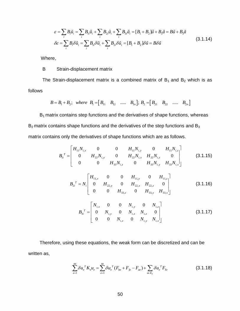
matrix contains only the derivatives of shape functions which are as follows.
11 , 11 , 11 ,
1 22 , 22 , 22 ,
33 , 33 , 33 ,
0 0 0
0 0 0
0 0 0
i x i y i z
T
i i y i x i z
i z i y i x
H N H N H N
B H N H N H N
H N H N H N
(3.1.15)
11, 11, 11,
2 22, 22, 22,
33, 33, 33,
0 0 0
0 0 0
0 0 0
x y z
T
i i y x z
z y x
H H H
B N H H H
H H H
(3.1.16)
, , ,
3 , , ,
, , ,
0 0 0
0 0 0
0 0 0
i x i y i z
T
i i y i x i z
i z i y i x
N N N
B N N N
N N N
(3.1.17)
Therefore, using these equations, the weak form can be discretized and can be
written as,
1 1
( )T
ne neT T T
e e e e be fe ae e Te
e e e E
u K u u F F F u F
(3.1.18)

51
Where,
1
1
( )2
e
T
e
hK B CB d d
(3.1.19)
1
1
( )2
e
T
be b
hF N F d d
(3.1.20)
e
T
feF N fd
(3.1.21)
1
3
1
( )2
e
T
ae
hF B CB a d d
(3.1.22)
1
0
1
12
e
e
T tTe
dhF N T d d
d
(3.1.23)
Where,
eK - Stiffness Matrix
e - Domain of integration
TE - Set of elements whose edge is with traction boundary condition
For the elements which is completely inside the boundary, that is, for internal
elements, the strain-displacement matrix 3B B . Therefore, the stiffness matrix
becomes,
1 1
3 3 3 3
11 1
( ) ( )2 2
t
e i
nT T
e
i A
h hK B CB d d B CB d dA
(3.1.24)
Where,
3B - Strain-displacement matrix which contains only the derivatives of
shape functions
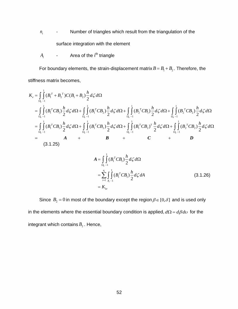
52
tn - Number of triangles which result from the triangulation of the
surface integration with the element
iA - Area of the ith triangle
For boundary elements, the strain-displacement matrix 1 2B B B . Therefore, the
stiffness matrix becomes,
1
1 2 1 2
1
1 1 1 1
1 1 1 2 2 1 2 2
1 1 1 1
1 1 1
1 1 1 2 1 2 2 2
1 1 1
( ) ( )2
( ) ( ) ( ) ( )2 2 2 2
( ) ( ) ( ) ( )2 2 2 2
e
e e e e
e e
T T
e
T T T T
T T T T T
hK B B C B B d d
h h h hB CB d d B CB d d B CB d d B CB d d
h h h hB CB d d B CB d d B CB d d B CB d d
1
1e e
A B C D
(3.1.25)
1
1 1
1
1
1 1
1 1
1
( )2
( )2
e
t
i
T
nT
i A
e
hB CB d d
hB CB d dA
K
A
(3.1.26)
Since 2 0B in most of the boundary except the region [0, ] and is used only
in the elements where the essential boundary condition is applied, d d d for the
integrant which contains 2B . Hence,
53
1
0
1
1 2
1
1
1 2
1
1
1 21
0
2
( )2
( )2
2
e
e
e
e
T
T
T
e
hB CB d d
hB CB d d d
hB CB d d d
K
B
(3.1.27)
1
0
1
1 2
1
1
1 2
1
1
1 21
0
2
( )2
( )2
2
e
e
e
e
T T
T T
T
T
T
e
hB CB d d
hB CB d d d
hB CB d d d
K
C
(3.1.28)
1
0
1
2 2
1
1
2 2
1
1
2 21
0
3
( )2
( )2
2
e
e
e
e
T
T
T
e
hB CB d d
hB CB d d d
hB CB d d d
K
D
(3.1.29)
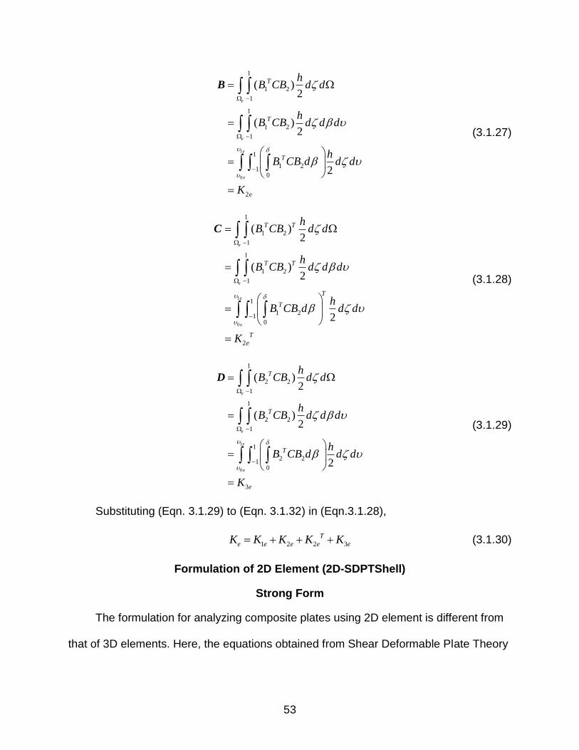
Substituting (Eqn. 3.1.29) to (Eqn. 3.1.32) in (Eqn.3.1.28),
1 2 2 3
T
e e e e eK K K K K (3.1.30)
Formulation of 2D Element (2D-SDPTShell)
Strong Form
The formulation for analyzing composite plates using 2D element is different from
that of 3D elements. Here, the equations obtained from Shear Deformable Plate Theory

54
(SDPT) are used. The inertial terms in Eqn (2.4.4) are eliminated and can be written in
Matrix form. The first two equations of Eqn (2.4.4) can be written as
0
0
0
x
x
y
y
xy
Npx y
Np
Ny x
The last two equations of Eqn (2.4.4) can be written as
0
0
0
x
x
y
y
xy
MQx y
MQ
My x
The third equation of Eqn (2.4.4) can be written as
0x
z
y
Qp
Qx y
The above Matrix equations can be simplified as
0TL N p (3.2.1)
0TL M Q (3.2.2)
0T p Q (3.2.3)
Where,
0
0 ; ;x
y
xp
Lpy
y x
p
And

55
2 2
2 2
h hx x x
y y y
h h
xy xy xy
N
N dz Q dz L
N
N A u (3.2.4)
2 2
2 2
h hx x x
y y y
h h
xy xy xy
M
M z dz zQ dz L
M
M D (3.2.5)
2
2
( )
h
x xz
s
y yzh
Qdz w
Q
Q A (3.2.6)
Substituting Eqns (3.2.4) and (3.2.5) in Eqns (3.2.1) and (3.2.2) respectively,
0TL L A u p (3.2.7)
0TL L D Q (3.2.8)
From Eqn (3.2.3),
0T p Q (3.2.9)
From Eqn (3.2.6),
1
0s
w QA
(3.2.10)
Weak Form
The above four equations Eqn (3.2.7) to Eqn (3.2.10) are the governing equations
which are used for further formulation. To these equations, the weighted residual
method is applied and simplified using Green’s formula to obtain the weak form. After
applying weighted residual method and Green’s Theorem, the weak form obtained is as
follows.

56
ˆ ˆ [( ) ( )] [ ] 0
ˆ ˆ [( ) ( )] [ ] 0
ˆ ( ) [ ] 0
10
P
Q
R
T T T T
P
T T T T
Q
T T
R
T T T
s
d L L d d
d L L d d
w d w d w p d
wd d d
u N n u u A u u p
M n D Q
Q Q
Q Q Q QA
(3.2.11)
Where,
ˆPN - Known traction (natural boundary condition) on the boundary P
ˆQM - Known moment (natural boundary condition) on the boundary Q
ˆRQ - Known shear (natural boundary condition) on the boundary R
To solve these equations, a three – field mixed formulation is used. The following
substitutions are made to solve it using mixed formulation.
ˆ ˆˆ ˆ, , ,
ˆ ˆˆ ˆ, , ,
u w Q
u w Q
w
w
u N u N w N Q N Q
u N u N w N Q N Q (3.2.12)
The shape functions , w QandN N N are formulated based on the number of
,wand Q parameters.
Using the above expression and simplifying the weak form, the matrix equation of
the final weak form becomes,
.T d
B DB X f (3.2.13)
Where,

57
ˆ0 0 0
ˆ0 0 ; 0 ; ; .
ˆ0 0 0
uu
w
Q w Q S
L
L
fN A B u
B N D B D X w f f
N X N X A f
Stiffness Matrix
From the above equation, it is clear that the stiffness matrix of the system of
equations depends upon , andA B D matrices and takes the form,
11 12 16 11 12 16
12 22 23 12 22 26
16 26 66 16 26 66
11 12 16 11 12 16
12 22 23 12 22 23
16 26 66 16 26 66
44 45
45 55
0 0
0 0
0 00
0 00
0 00 0
0 0
0 0 0 0 0 0
0 0 0 0 0 0
S
A A A B B B
A A A B B B
A A A B B B
B B B D D D
B B B D D D
B B B D D D
A A
A A
A B
K D B D
A
(3.2.14)

58
CHAPTER 4 FINITE ELEMENT FORMULATION FOR COMPOSITE PLATES
In the composite Laminate, the property of the laminate differ layer wise. Each layer
has a different material property which depends upon the Young’s Modulus, Shear
Modulus and Poisson’s ratio of the fiber and matrix, fiber orientation etc. The property of
the laminate also depends upon the thickness of the lamina. Hence, the calculation of
stiffness matrix is different from those of Isotropic materials.
The stiffness of the laminate can be determined by the Laminate constitutive relations
(Eqn. 2.3.26 and Eqn. 2.4.11). The first equation (Eqn. 2.3.26) gives the laminate
constitutive relation derived using Classical Lamination Plate Theory, in which the
transverse normal and shear forces are neglected and hence the transverse shear
strains are negligible.
As this theory holds good for only thinner plates and shells, another theory was
developed which considers the transverse normal and shear stresses into
consideration and takes shear strains into account while calculating the maximum
deflection of the plate for applied load, which is known as Shear Deformable Plate
Theory. From this Theory, the constitutive equation of the laminate is derived which is
given in Eqn 2.4.11. From this relation, the stiffness matrix of the laminate is found.
When the two laminate constitutive relations are observed, the stiffness matrix of the
laminate depends upon 3 matrices, In-plane Stiffness Matrix [A], Bending Stiffness
matrix [D] and coupling Stiffness Matrix [B]. Hence, to calculate the laminate stiffness,
we need to determine all these three matrices. After the 3 matrices are calculated, the
equivalent stiffness matrix of the laminate is calculated in two different ways. This is
shown in two different elements used in IBFEM. They are 3D-Shell and 2D-SDPTShell.

59
In the 3D-Shell, the weak form is derived from the stress-strain relation and hence the
stiffness matrix is obtained from the stress-strain relation of the laminate. Since, the
stiffness matrix of the laminate is not directly available from the stress-strain relation of
the laminate; the equivalent stiffness of the laminate is obtained from the Reduced
Bending Stiffness Matrix [Dr] which is derived from the in-plane stiffness matrix [A],
coupling stiffness matrix [B] and bending stiffness matrix [D]. This may increase the
percentage of error as well as the computational time. To overcome these difficulties,
another element is developed which is known as 2D-SDPTShell in which the weak form
is formulated from the equations obtained from Shear-Deformable Plate Theory (SDPT).
Since the weak form is formulated from the Force/Moment-Strain/curvature relation,
from the in-plane stiffness matrix [A], coupling stiffness matrix [B] and bending stiffness
matrix [D] can be directly used in the formulation. Then the error percentages of the
results obtained from these two elements are compared and the best element used for
composite plates is concluded. This shows that the error percentage and computational
time is better than the other element. It also converges faster, (i.e.) in a very low mesh
density than the other elements which is clearly shown from the convergence plots. The
following chapter explains the computation of the stiffness matrix for each element.
Stiffness Matrix in 3D-Shell Element
The explanation of calculation of stiffness matrix which is used in 3D-Shell element
involves first the determination of bending stiffness matrix for only symmetric laminates
followed by generalized determination of bending stiffness matrix for laminates. First,
the stiffness matrix of each layer in the material direction is calculated. Then it is
transformed to global co-ordinates. It is followed by combining the transformed stiffness
of each layer to obtain the stiffness of the whole laminate.

60
Input Parameters
The parameters which we need to calculate the stiffness matrix are collected
from the user through the graphical interface which is used in IBFEM. The properties
are different for different lamina and these properties are collected for each and every
layer. The properties which we need for each layer are as follows.
1. Young's Modulus along the direction of the fiber - E1
2. Young's Modulus perpendicular to the direction of the fiber - E2
3. Young's Modulus along the transverse direction of the fiber - E3
4. Poisson's Ratio of transverse strain in 2-direction to axial strain in 1-direction - ϒ12
5. Poisson's Ratio of transverse strain in 3-direction to axial strain in 2-direction - ϒ23
6. Poisson's Ratio of transverse strain in 3-direction to axial strain in 1-direction - ϒ13
7. Shear Modulus in 1-2 plane - G12
8. Shear Modulus in 2-3 plane - G23
9. Shear Modulus in 1-3 plane - G13
Stiffness Matrix of Each Layer in Material Direction (1-2 direction)
Here, each lamina is considered as an orthotropic material whose material
properties are collected. The stiffness Matrix of each layer is calculated from the stress-
strain relation as follows.
1 111 12
2 12 22 2
6612 12
0
0
0 0
S S
S S
S
(4.1.1)
From this relation, the compliance matrix [S] is given as
11 12
12 22
66
0
0
0 0
S S
S S S
S
(4.1.2)

61
Where,
From [S] matrix, the stiffness matrix [Q] is determined by,
1[ ] [ ]Q S
Stiffness Matrix of Each Layer in Global Co-ordinates (X-Y Direction)
Since the fiber direction is different for each layer, the stiffness matrix of each
layer is different and it depends upon the direction of the fiber. To calculate the total
stiffness of the laminate, the stiffness matrix of each layer should be transformed to a
global co-ordinate system. For convenience, they are all transformed to global direction
in which the plate or shell is aligned. Hence, the stiffness matrix of each layer is
multiplied with the transformation matrix to align it with the global co-ordinate system.
The transformation matrix is given by
2 2
2 2
2 2
2
2
where, m = cos , n = sin
m n mn
T n m mn
mn mn m n
(4.1.3)
And the transformed stiffness matrix of a single layer [ ̅] = [T] [Q] [T] T is given by
11 12 16
12 22 26
16 26 66
Q Q Q
Q Q Q Q
Q Q Q
(4.1.4)
Combined Bending Stiffness of the Laminate
To find the stiffness of the whole laminate, the stiffness matrix of each layer
should be combined together. This can be done by finding the combined bending
stiffness of the laminate and convert it into stiffness matrix.
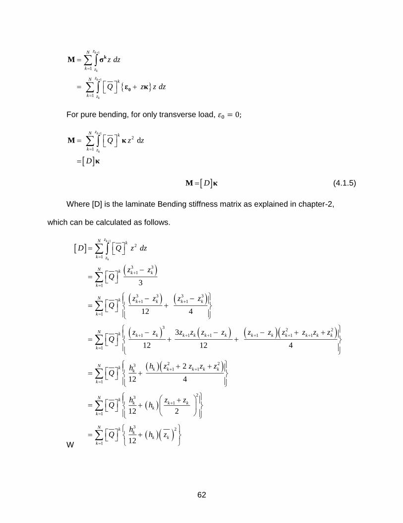
From the moment equation,
21 211 22 12 66 21 12
1 2 2 12 1
1 1 1; ; ; ; ;
ES S S S
E E E G E
62
1
1
1
1
k
k
k
k
zN
k z
zN k
k z
z dz
Q z z dz
k
0
M σ
ε κ
For pure bending, for only transverse load, =
1
2
1
d
k
k
zN k
k z
Q z z
D
M
κ
κ
DM κ (4.1.5)
Where [D] is the laminate Bending stiffness matrix as explained in chapter-2,
which can be calculated as follows.
W
1
2
1
3 3 1
1
3 3 3 3
1 1
1
3
2 2
1 1 1 1 1 1
1
3
12 4
3
12 12 4
k
k
zN k
k z
N k k k
k
N k k k k k
k
N k k k k k k k k k k k k k
k
D Q z dz
z zQ
z z z zQ
z z z z z z z z z z z zQ
2 23
1 1
1
2
3
1
1
3
2
1
2
12 4
12 2
12
N k k k k k kk
k
N kk k k
k
k
N kk
k k
k
h z z z zhQ
h z zQ h
hQ h z

63
32
1
12
N kk
k k
k
hD Q h z
(4.1.6)
where,
1
- Thickness of each layer
Z - z co-ordinate of mid of each layer2
k
k kk
h
Z Z
Therefore [D] matrix takes the form,
11 12 16
12 22 26
16 26 66
[ ]
D D D
D D D D
D D D
(4.1.7)
Approximation for Unsymmetrical Laminates
Unsymmetrical laminates are the one in which the in-plane stresses are developed
when the plate is subjected to only transverse load. This is because of the anisotropic
property of the laminate which can be seen from the emergence of [B] matrix for
unsymmetrical laminates. From Eqn 2.3.23 and Eqn. 2.3.24, the in-plane stress
resultants and moment resultants depends on all the three matrices (i.e.) [A], [B], and
[D] matrices. But for symmetric laminates, as the [B] matrix vanishes, the two equations
uncouple and it becomes easy to find the stiffness matrix of the laminate. But, for
unsymmetrical laminates, as the two equations are coupled to each other by [B] matrix,
it becomes important to consider all the three matrices when the stiffness of the
laminate is determined. Due to the existence of this coupling effect, (i.e.) existence of in-
plane stresses when the plane is subjected to only bending loads, the magnitude of
bending displacement gets reduced. This is because of the presence of in-plane
stiffness which reduces the bending stiffness. So the material gets stiffer due to the
reduction in the overall bending stiffness. This is known as Stress-Stiffening effect. So

64
the overall bending stiffness is reduced and is called Reduced Bending Stiffness Matrix
[Dr]. It can be calculated as follows.
From the first equation of the laminate constitutive equation,
A B 0N ε κ
A B 0ε N κ
Where [A] and [B] are called laminate stiffness matrices as explained in chapter-2,
which are individually known as follows:
[A]: In-plane stiffness matrix
[B]: Coupling stiffness matrix
These matrices are defined as,
2
1
/2
/2
1
1
11 12 16
12 22 26
16 26 66
[ ] [ ]
[ ]
[ ]
i
i
h
h
ZNL
i
i Z
NL
i i
i
A Q dz
Q dz
Q h
A A A
A A A
A A A
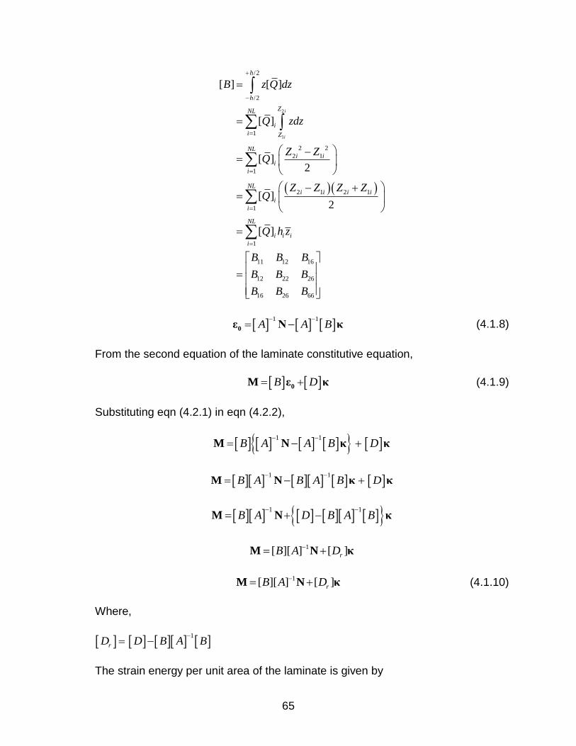
65
2
1
/2
/2
1
2 2
2 1
1
2 1 2 1
1
1
11 12 16
12 22 26
16 26 66
[ ] [ ]
[ ]
[ ]2
[ ]2
[ ]
i
i
h
h
ZNL
i
i Z
NLi i
i
i
NLi i i i
i
i
NL
i i i
i
B z Q dz
Q zdz
Z ZQ
Z Z Z ZQ
Q h z
B B B
B B B
B B B
1 1
A A B
0ε N κ (4.1.8)
From the second equation of the laminate constitutive equation,
B D 0M ε κ (4.1.9)
Substituting eqn (4.2.1) in eqn (4.2.2),
1 1
B A A B D
M N κ κ
1 1
B A B A B D
M N κ κ
1 1 B A D B A B
M N κ
1[ ][ ] [ ]rB A D M N κ
1[ ][ ] [ ]rB A D M N κ (4.1.10)
Where,
1
rD D B A B
The strain energy per unit area of the laminate is given by
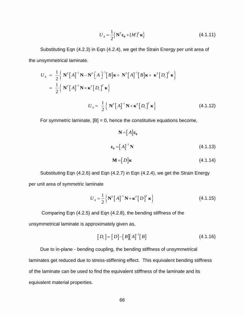
66
1
[ ]2
T T
AU M 0εN κ (4.1.11)
Substituting Eqn (4.2.3) in Eqn (4.2.4), we get the Strain Energy per unit area of
the unsymmetrical laminate.
11 1
1
1
2
1
2
TT T T T
A r
TT T
r
U A A B A B D
A D
N N N κ N κ κ κ
N N κ κ
11
2
TT T
A rU A D
N N κ κ (4.1.12)
For symmetric laminate, [B] = 0, hence the constitutive equations become,
A 0N ε
1
A
0ε N (4.1.13)
DM κ (4.1.14)
Substituting Eqn (4.2.6) and Eqn (4.2.7) in Eqn (4.2.4), we get the Strain Energy
per unit area of symmetric laminate
1
1
2
TT T
AU A D
N N κ κ (4.1.15)
Comparing Eqn (4.2.5) and Eqn (4.2.8), the bending stiffness of the
unsymmetrical laminate is approximately given as,
1
rD D B A B
(4.1.16)
Due to in-plane - bending coupling, the bending stiffness of unsymmetrical
laminates get reduced due to stress-stiffening effect. This equivalent bending stiffness
of the laminate can be used to find the equivalent stiffness of the laminate and its
equivalent material properties.

67
Therefore [Dr] matrix takes the form,
11 12 16
12 22 26
16 26 66
[ ]
r r r
r r r r
r r r
D D D
D D D D
D D D
(4.1.17)
Therefore, this reduced stiffness [Dr] can be used instead of the bending stiffness
[D] from which the stiffness matrix of the laminate can be determined.
Stiffness Matrix of the Laminate
If the whole laminate is considered as a single layer, becomes zero and hk
becomes the total thickness t. Therefore,
3
* 12
tD Q
*
3
12 Q D
t (4.1.18)
Hence, [Q*] is a 3x3 matrix from which [S*] is obtained which is as follows,
*
* * *
11 12 16
* * *
12 22 26
* * *
16 2
* 1
6 66
[ ]S
S S S
S S S
S S
Q
S
Hence, the equivalent material properties of the laminate is determined as,
* * *
11 22 66
1 1 1; ; ;x y xyE E G
S S S
* *
16 26, ,* *
12 12
; ; ; ;yx
xy yx xy x xy y
xy xy
EE S S
S S G G
From SDPT, the Shear stiffness matrix [As] is as follows.
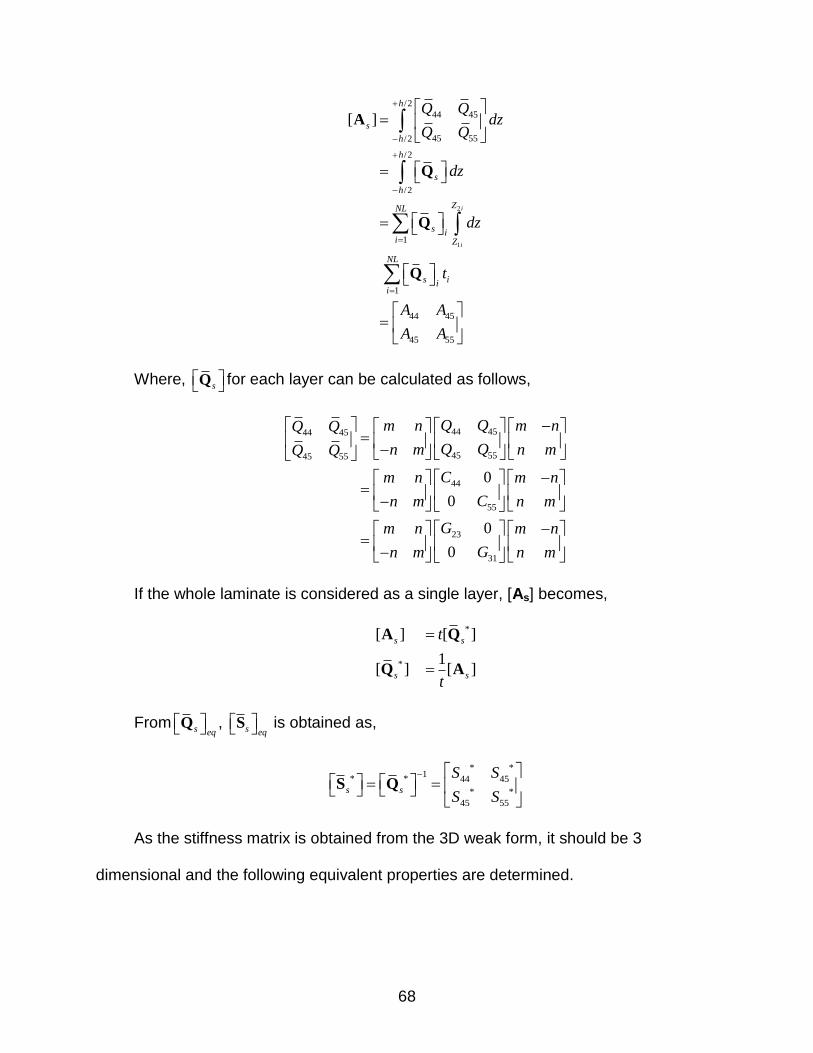
68
2
1
/2
44 45
45 55/2
/2
/2
1
1
44 45
45 55
[ ]
i
i
h
s
h
h
s
h
ZNL
s ii Z
NL
s iii
Q Qdz
Q Q
dz
dz
t
A A
A A
A
Q
Q
Q
Where, s
Q for each layer can be calculated as follows,
44 4544 45
45 5545 55
44
55
23
31
0
0
0
0
Q Qm n m nQ Q
Q Qn m n mQ Q
Cm n m n
Cn m n m
Gm n m n
Gn m n m
If the whole laminate is considered as a single layer, [As] becomes,
*
*
[ ] [ ]
1[ ] [ ]
s s
s s
t
t
A Q
Q A
From s eq Q , s eq
S is obtained as,
* *1
* * 44 45
* *
45 55
s s
S S
S S
S Q
As the stiffness matrix is obtained from the 3D weak form, it should be 3
dimensional and the following equivalent properties are determined.

69
3 * *
44 55
1 1; ; ;
1; 1; ; ;2 2
z yz xz
y x z zyz xz zy yz zx xz
yz xz y x
E E G GS S
E E E E
G G E E
To complete the equivalent 3D compliance matrix of the laminate, the following
terms are determined
* * *
33 13 23
1; ;
zyzx
z z z
S S SE E E
Therefore the equivalent 3D compliance matrix takes the form,
* * * *
11 12 13 16
* * * *
12 22 23 26
* * *
13 23 33
* *
44 45
* *
45 55
* * *
16 26 66
0 0
0 0
0 0 0[ ]
0 0 0 0
0 0 0 0
0 0 0
eq
S S S S
S S S S
S S SS
S S
S S
S S S
The equivalent stiffness matrix of the laminate is obtained as,
11 12 13 14 15 16
12 22 23 24 25 26
13 23 33 34 35 36
14 24 34 44 45 46
15 25 35 45 55 56
16 26 36 46 56 66
1
eq eqS
d d d d d d
d d d d d d
d d d d d d
d d d d d d
d d d d d d
d d
Q
d d d d
(4.1.19)
Stiffness Matrix in 2D-SDPTShell
The equivalent stiffness matrix used in 2D-SDPTShell element is directly obtained
from in-plane, coupling and bending stiffness matrices. Since this element is formulated
using Shear Deformable Plate Theory, it also considers transverse normal and shear

70
forces and the transverse shear strains are also considered. Hence, the formulation of
stiffness matrix includes another 3 new terms A44, A45, and A55 which is obtained from
the constitutive relations of the shear stress and strains. The formulation of equivalent
stiffness matrix used in 2D-SDPTShell is as follows.
Equivalent Stiffness Matrix
From the constitutive relation of the laminate using Shear Deformable Plate
Theory,
s
N A B 0
M B D 0
0 0 A
sQ
0
s
ε
γ
(4.2.1)
Where [A], [B], [D] and [As] are known as follows:
[A]: In-plane stiffness matrix
[B]: Coupling stiffness matrix
[D]: Bending stiffness matrix
[As]: Shear stiffness matrix
These matrices are defined as,
11 12 16/2
12 22 26
/2
16 26 66
11 12 16/2
12 22 26
/2
16 26 66
11 12 16/2
2
12 22 26
/2
16 26 66
44 45
45 55/2
[ ] [ ]
[ ] [ ]
[ ] [ ]
[ ]
h
h
h
h
h
h
s
h
A A A
A Q dz A A A
A A A
B B B
B z Q dz B B B
B B B
D D D
D z Q dz D D D
D D D
Q Qdz
Q Q
A
/244 45
45 55
h A A
A A
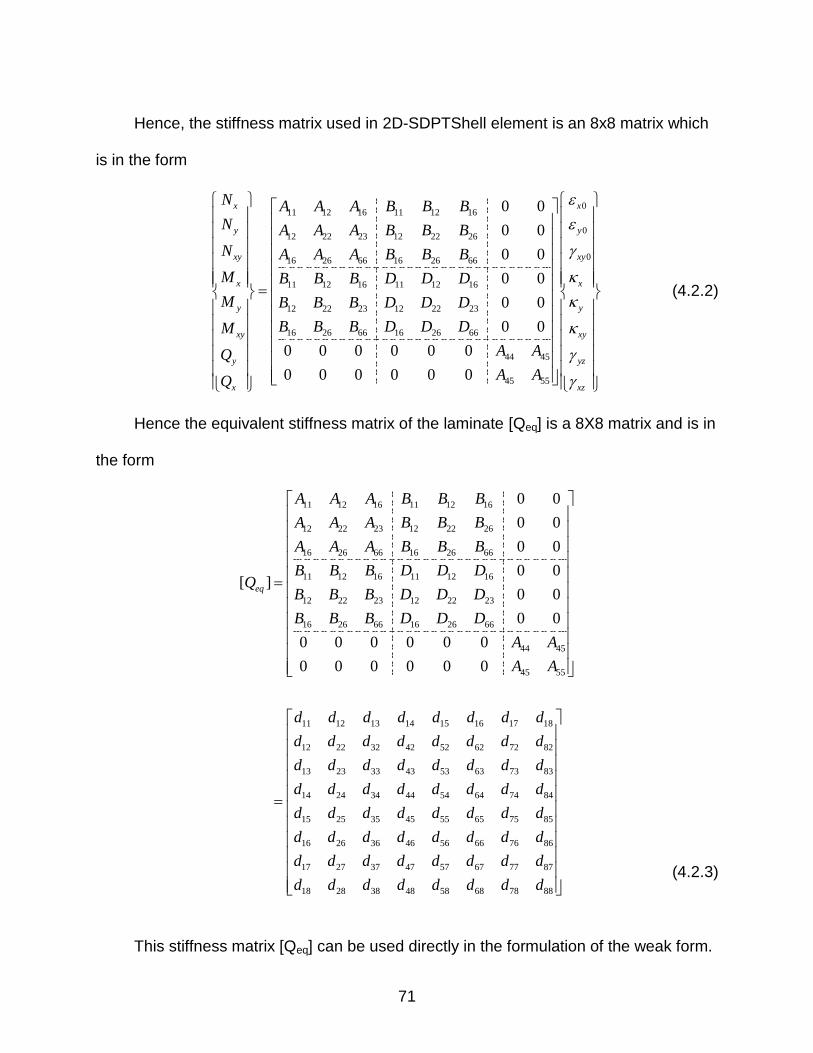
71
Hence, the stiffness matrix used in 2D-SDPTShell element is an 8x8 matrix which
is in the form
11 12 16 11 12 16
12 22 23 12 22 26
16 26 66 16 26 66
11 12 16 11 12 16
12 22 23 12 22 23
16 26 66 16 26 66
44 45
45 55
0 0
0 0
0 0
0 0
0 0
0 0
0 0 0 0 0 0
0 0 0 0 0 0
x
y
xy
x
y
xy
y
x
N A A A B B BN A A A B B B
N A A A B B B
M B B B D D D
M B B B D D D
B B B D D DM
A AQ
A AQ
0
0
0
x
y
xy
x
y
xy
yz
xz
(4.2.2)
Hence the equivalent stiffness matrix of the laminate [Qeq] is a 8X8 matrix and is in
the form
11 12 16 11 12 16
12 22 23 12 22 26
16 26 66 16 26 66
11 12 16 11 12 16
12 22 23 12 22 23
16 26 66 16 26 66
44 45
45 55
11 12 13 14 15 16 17 1
0 0
0 0
0 0
0 0[ ]
0 0
0 0
0 0 0 0 0 0
0 0 0 0 0 0
eq
A A A B B B
A A A B B B
A A A B B B
B B B D D DQ
B B B D D D
B B B D D D
A A
A A
d d d d d d d d
8
12 22 32 42 52 62 72 82
13 23 33 43 53 63 73 83
14 24 34 44 54 64 74 84
15 25 35 45 55 65 75 85
16 26 36 46 56 66 76 86
17 27 37 47 57 67 77 87
18 28 38 48 58 68 78 88
d d d d d d d d
d d d d d d d d
d d d d d d d d
d d d d d d d d
d d d d d d d d
d d d d d d d d
d d d d d d d d
(4.2.3)
This stiffness matrix [Qeq] can be used directly in the formulation of the weak form.

72
CHAPTER 5 RESULTS AND DISCUSSION
In order to check the method which have been used to analyze composite plates
and shells and to authenticate the application of B-spline Finite Element Method and
SDPT Composite Plates and shells, few standard examples which include composite
beams, square plates, Composite Wing and Composite plate with a hole have been
used. In the following chapter, the structural analysis of composite plates is done using
two types of elements which have been formulated using two different methods. In the
discussion, the element named 3D-Shell is a 3D element and is formulated using B-
Spline Finite Element Method. The element named 2D-SDPTShell is a 2D element and
is formulated using equation from Shear Deformable Plate Theory (SDPT) considering
the concept of constant transverse shear force throughout the thickness of the plate.
This chapter is mainly to find the difference among the elements developed and to
conclude which element is the best for which cases as well as for the future research.
Example 1: Composite Beam
A 1-D composite plate [23] whose width is small when compared to the length and
the applied load varies in only one direction is shown in Figure 5-1. The plate has
dimension 1 X 0.1 m2 and is loaded with an uniformly distributed load(UDL) of 1000 Pa
transversely. The material properties used are:
E1 = 225 GPa, 2 9.0E GPa , 12 0.3 , G12 = G13 = 6.9 GPa, G23 = 3 GPa.
The beam is analyzed with 3 types of boundary conditions, Hinged-Hinged (HH),
Clamped-Clamped (CC) and Clamped-Free (CF) and the results obtained using
Traditional Finite Element Method is compared with the analytical results.

73
Figure 5-1. Composite beam
A B C
Figure 5-2. Mesh pattern for Composite beam. A) Traditional FEA (abaqus). B) 3D-Shell. C) 2D-SDPTShell
A B C
Figure 5-3. Traditional FEA (abaqus) results of Composite beam. A) Hinged-Hinged. B) Clamped-Clamped. C) Clamped-Free
0.1
1

74
A B C
Figure 5-4. 3D-Shell results of Composite beam. A) Hinged-Hinged. B) Clamped-Clamped. C) Clamped-Free
A B C
Figure 5-5. 2D-SDPTShell results of Composite beam. A) Hinged-Hinged. B)
Clamped-Clamped. C) Clamped-Free
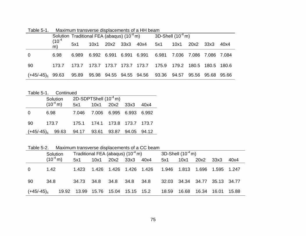
75
Table 5-1. Maximum transverse displacements of a HH beam
Solution (10-4
m)
Traditional FEA (abaqus) (10-4 m) 3D-Shell (10-4 m)
5x1 10x1 20x2 33x3 40x4 5x1 10x1 20x2 33x3 40x4
0 6.98 6.989 6.992 6.991 6.991 6.991 6.981 7.036 7.086 7.086 7.084
90 173.7 173.7 173.7 173.7 173.7 173.7 175.9 179.2 180.5 180.5 180.6
(+45/-45)s 99.63 95.89 95.98 94.55 94.55 94.56 93.36 94.57 95.56 95.68 95.66
Table 5-1. Continued
Solution (10-4 m)
2D-SDPTShell (10-4 m)
5x1 10x1 20x2 33x3 40x4
0 6.98 7.046 7.006 6.995 6.993 6.992
90 173.7 175.1 174.1 173.8 173.7 173.7
(+45/-45)s 99.63 94.17 93.61 93.87 94.05 94.12
Table 5-2. Maximum transverse displacements of a CC beam
Solution (10-4 m)
Traditional FEA (abaqus) (10-4 m) 3D-Shell (10-4 m)
5x1 10x1 20x2 33x3 40x4 5x1 10x1 20x2 33x3 40x4
0 1.42 1.423 1.426 1.426 1.426 1.426 1.946 1.813 1.696 1.595 1.247
90 34.8 34.73 34.8 34.8 34.8 34.8 32.03 34.34 34.77 35.13 34.77
(+45/-45)s 19.92 13.99 15.76 15.04 15.15 15.2 18.59 16.68 16.34 16.01 15.88

76
Table 5-2. Continued
Solution (10-4 m)
2D-SDPTShell (10-4 m)
5x1 10x1 20x2 33x3 40x4
0 1.42 1.48 1.44 1.43 1.427 1.427
90 34.8 36.15 35.18 34.9 34.85 34.83
(+45/-45)s 19.92 13.85 14.43 14.75 14.92 14.98
Table 5-3. Maximum transverse displacements of a CF beam
Table 5-3. Continued
Solution (10-4 m)
Traditional FEA (abaqus) (10-4 m) 3D-Shell(10-4 m)
5x1 10x1 20x2 33x3 40x4 5x1 10x1 20x2 33x3 40x4
0 67 66.8 66.8 66.8 66.8 66.8 79.68 76.18 72.83 67.84 62.68
90 1670 1666 1667 1667 1667 1667 1667 1667 1667 1674 1667
(+45/-45)s 954 805.3 845.7 829.7 832.7 834 921.2 871.6 861.2 853.6 850.5
Solution (10-4 m)
2D-SDPTShell(10-4 m)
5x1 10x1 20x2 33x3 40x4
0 67 67.01 66.83 66.79 66.78 66.78
90 1670 1673 1668 1667 1667 1667
(+45/-45)s 954 795.7 812.8 821.4 826.3 828.2

77
A
B
Figure 5-6. Convergence plots of Hinged-Hinged beam. A) 0. B) 90. C) (+45/-45)s

78
C
Figure 5-6. Continued
A
Figure 5-7. Convergence plots of Clamped-Clamped beam. A) 0. B) 90. C) (+45/-45)s

79
B
C
Figure 5-7. Continued
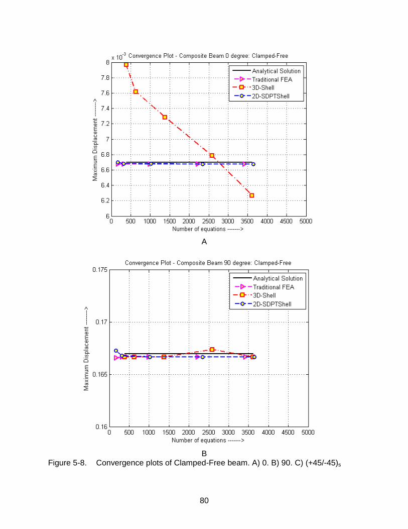
80
A
B
Figure 5-8. Convergence plots of Clamped-Free beam. A) 0. B) 90. C) (+45/-45)s

81
C
Figure 5-8. Continued

82
Example 2: Square Composite Plate
A square composite plate [23] of dimension 1X1 m2 with thickness 0.01 m is
subjected to uniform pressure of 1000 Pa and its maximum deflection at the center is
determined. The material properties used are:
E1 = 225 GPa, E2 = 9 GPa, ϒ12 = 0.25, G12 = G13 = 4.5 GPa, G23 = 1.8 GPa.
It is simply supported on all its edges (i.e.) at x = -0.5 and 0.5, v0 = w0 = Mxx = 0 &
at y = -0.5 and 0.5, u0 = wo = Myy = 0. Using these boundary conditions and material
properties, results are obtained using traditional FEA (abaqus) and are compared with
the analytical solutions.
Figure 5-9. Composite square plate
1 1
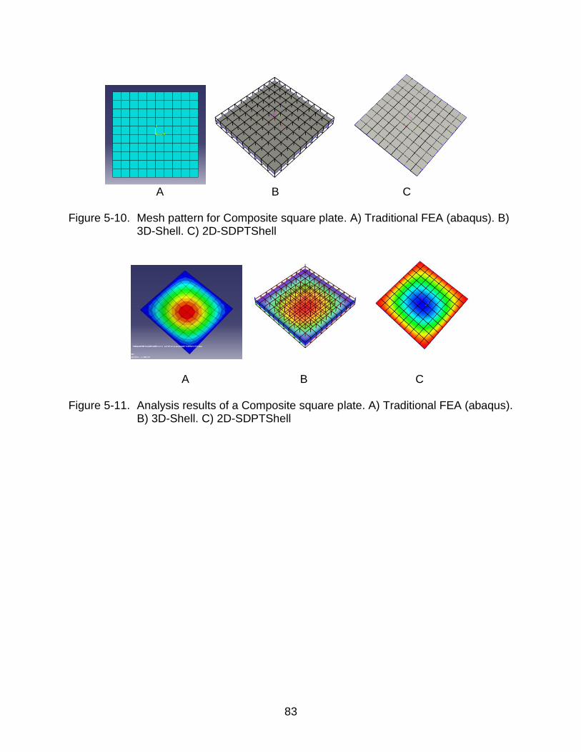
83
A B C
Figure 5-10. Mesh pattern for Composite square plate. A) Traditional FEA (abaqus). B) 3D-Shell. C) 2D-SDPTShell
A B C
Figure 5-11. Analysis results of a Composite square plate. A) Traditional FEA (abaqus). B) 3D-Shell. C) 2D-SDPTShell
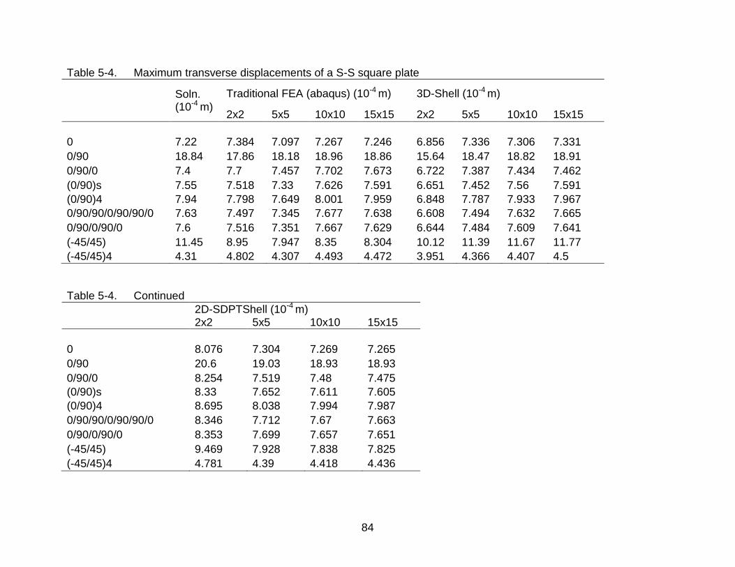
84
Table 5-4. Maximum transverse displacements of a S-S square plate
Soln. (10-4 m)
Traditional FEA (abaqus) (10-4 m) 3D-Shell (10-4 m)
2x2 5x5 10x10 15x15 2x2 5x5 10x10 15x15
0 7.22 7.384 7.097 7.267 7.246 6.856 7.336 7.306 7.331
0/90 18.84 17.86 18.18 18.96 18.86 15.64 18.47 18.82 18.91
0/90/0 7.4 7.7 7.457 7.702 7.673 6.722 7.387 7.434 7.462
(0/90)s 7.55 7.518 7.33 7.626 7.591 6.651 7.452 7.56 7.591
(0/90)4 7.94 7.798 7.649 8.001 7.959 6.848 7.787 7.933 7.967
0/90/90/0/90/90/0 7.63 7.497 7.345 7.677 7.638 6.608 7.494 7.632 7.665
0/90/0/90/0 7.6 7.516 7.351 7.667 7.629 6.644 7.484 7.609 7.641
(-45/45) 11.45 8.95 7.947 8.35 8.304 10.12 11.39 11.67 11.77
(-45/45)4 4.31 4.802 4.307 4.493 4.472 3.951 4.366 4.407 4.5
Table 5-4. Continued
2D-SDPTShell (10-4 m) 2x2 5x5 10x10 15x15
0 8.076 7.304 7.269 7.265
0/90 20.6 19.03 18.93 18.93
0/90/0 8.254 7.519 7.48 7.475
(0/90)s 8.33 7.652 7.611 7.605
(0/90)4 8.695 8.038 7.994 7.987
0/90/90/0/90/90/0 8.346 7.712 7.67 7.663
0/90/0/90/0 8.353 7.699 7.657 7.651
(-45/45) 9.469 7.928 7.838 7.825
(-45/45)4 4.781 4.39 4.418 4.436
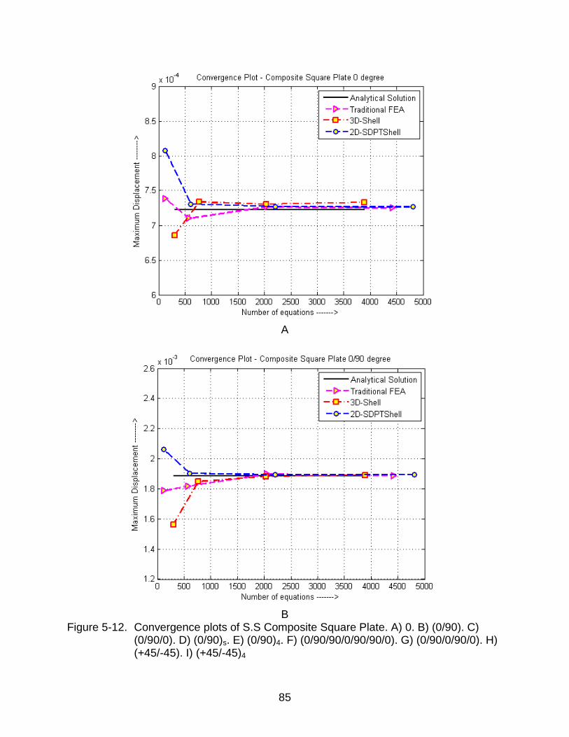
85
A
B
Figure 5-12. Convergence plots of S.S Composite Square Plate. A) 0. B) (0/90). C) (0/90/0). D) (0/90)s. E) (0/90)4. F) (0/90/90/0/90/90/0). G) (0/90/0/90/0). H) (+45/-45). I) (+45/-45)4

86
C
D
Figure 5-12. Continued

87
E
F
Figure 5-12. Continued

88
G
H
Figure 5-12. Continued

89
I
Figure 5-12. Continued

90
Example 3: Composite Wing of Micro-Air Vehicle
Micro-Air Vehicles (MAV's) are UAV's of comparatively small size which have
been used for several applications such as surveillance, bird-flight or insect-flight study
and aerial photography. In this case, a MAV wing is taken for analysis which is made
up of Carbon-Epoxy Composite Laminate whose material properties are:
1 2 3 12 13 23
12 13 23
= 181GPa; E E = 10.3GPa; 0.28; 0.0159;
G G 7.17GPa; G 5.07GPa
E
The wing is clamped at one edge. Therefore the boundary conditions are:
At one edge,(x=0); 0x y zu v w
It is made up of (±26.5)s laminate with lamina thickness of 0.125mm. It is
subjected to uniform pressure of 1Pa and the maximum deflection is determined.
Figure 5-13. Composite wing
A B C
Figure 5-14. Mesh pattern for composite wing. A) Traditional FEA (abaqus). B) 3D-
Shell. C) 2D-SDPTShell
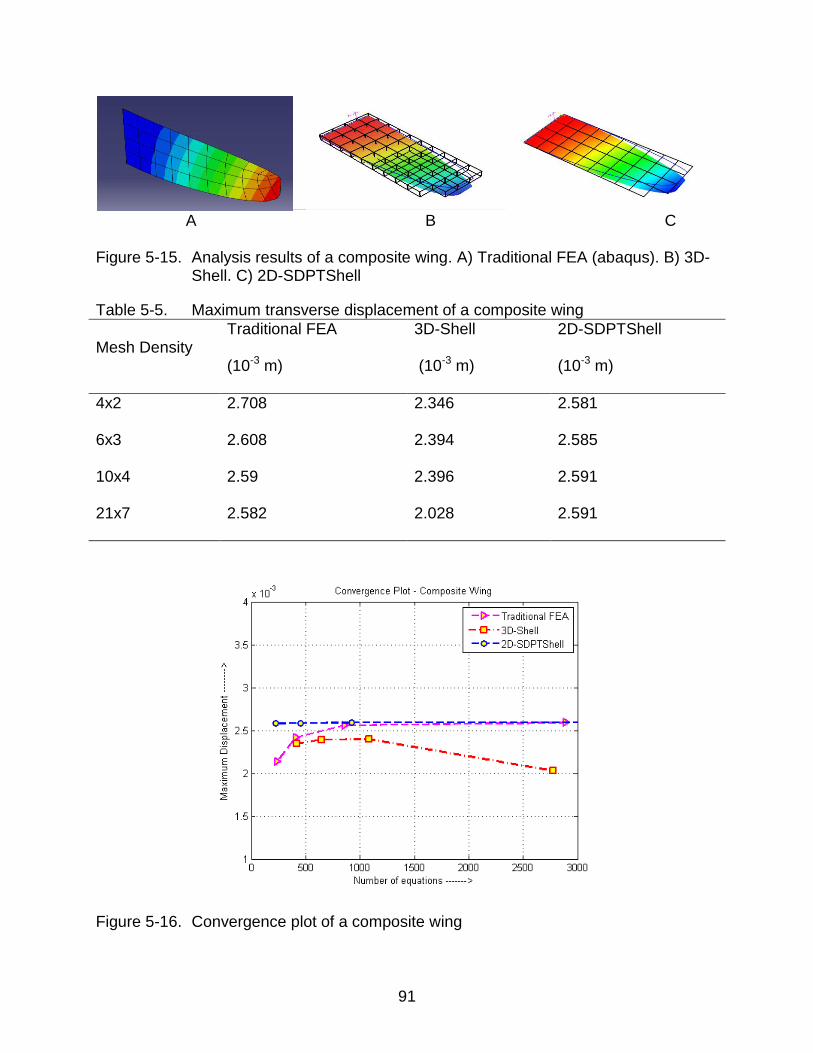
91
A B C
Figure 5-15. Analysis results of a composite wing. A) Traditional FEA (abaqus). B) 3D-
Shell. C) 2D-SDPTShell
Table 5-5. Maximum transverse displacement of a composite wing
Mesh Density Traditional FEA
(10-3 m)
3D-Shell
(10-3 m)
2D-SDPTShell
(10-3 m)
4x2 2.708 2.346 2.581
6x3 2.608 2.394 2.585
10x4 2.59 2.396 2.591
21x7 2.582 2.028 2.591
Figure 5-16. Convergence plot of a composite wing

92
Example 4: Composite Plate with a Hole
A composite plate of size 2 X 2 m2 with a hole of diameter 1 m at the center is
subjected to uniform pressure load of 100 Pa and its maximum displacement is
determined. This plate is simply supported at all the 4 edges (i.e.) at x = -1 and 1, v0 =
w0 = 0 & at y = -1 and 1, u0 = wo = 0. The mechanical properties of the laminate of
thickness 0.012 m are as follows:
E1 = 130 GPa, E2 = E3 = 10 GPa, ϒ12 = 0.35, G12 = G13 = 5 GPa, G23 = 3.7 GPa
Figure 5-17. Composite plate with a hole
Two types of stacking sequences, which are (i) [0/90]2s and (ii) [452/90/0]s are
tested and analyzed. The Traditional FEA results using Abaqus are extracted and
compared with the IBFEM results from two types of elements developed and the
method explained in this thesis is validated.
2
2 1

93
A B C
Figure 5-18. Mesh pattern for composite plate with a hole. A) Traditional FEA (abaqus),
B) 3D-Shell. C) 2D-SDPTShell
A B C
Figure 5-19. Analysis results of Composite plate with a hole. A) Traditional FEA (abaqus) results. B) 3D-Shell results. C) 2D-SDPTShell results
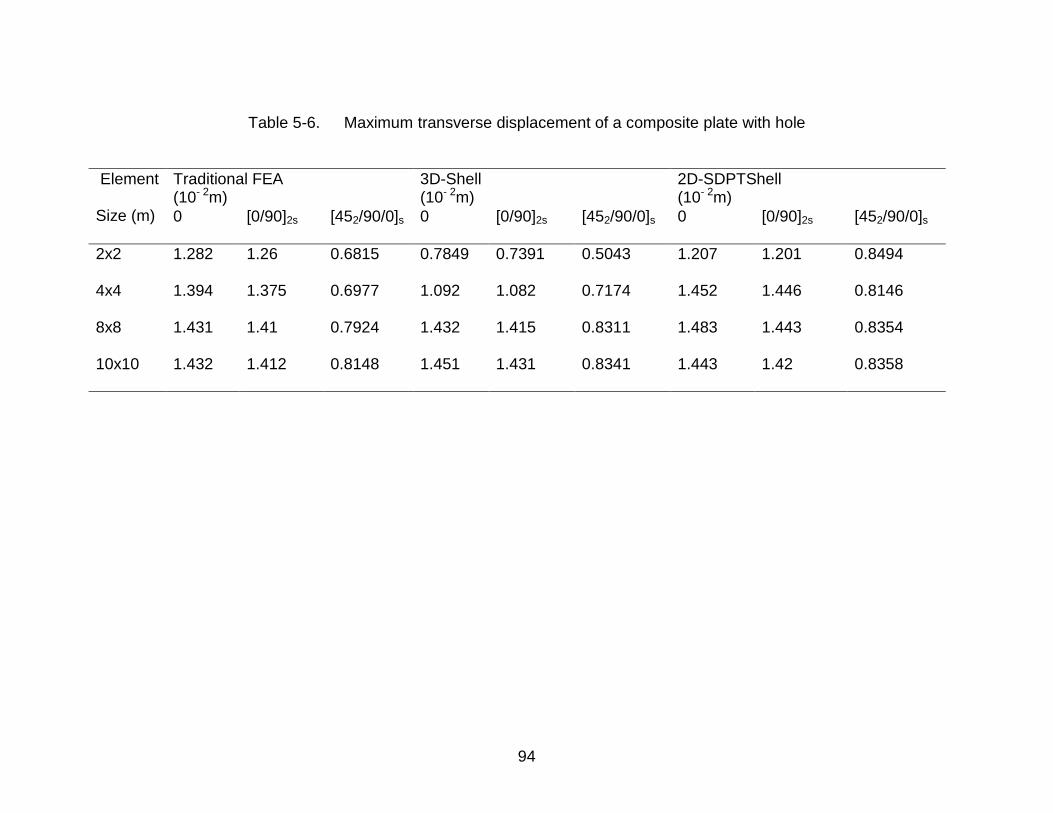
94
Table 5-6. Maximum transverse displacement of a composite plate with hole
Element
Size (m)
Traditional FEA (10- 2m)
3D-Shell (10- 2m)
2D-SDPTShell (10- 2m)
0 [0/90]2s [452/90/0]s 0 [0/90]2s [452/90/0]s 0 [0/90]2s [452/90/0]s
2x2 1.282 1.26 0.6815 0.7849 0.7391 0.5043 1.207 1.201 0.8494
4x4 1.394 1.375 0.6977 1.092 1.082 0.7174 1.452 1.446 0.8146
8x8 1.431 1.41 0.7924 1.432 1.415 0.8311 1.483 1.443 0.8354
10x10 1.432 1.412 0.8148 1.451 1.431 0.8341 1.443 1.42 0.8358
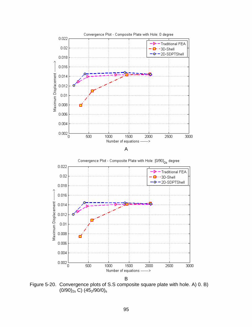
95
A
B
Figure 5-20. Convergence plots of S.S composite square plate with hole. A) 0. B) (0/90)2s C) (452/90/0)s

96
C
Figure 5-20. Continued
.

97
CHAPTER 6 CONCLUSION
Summary
In this thesis, the use of IBFEM to model composite plates is studied. Initially the
equations required for general formulation of Finite Element Method in laminated
composites is explained. It includes the derivation of equations used in FEM formulation
using Classical Lamination Plate Theory (CLPT) and Shear Deformable Plate Theory
(SDPT). This is followed by an introduction to the Implicit Boundary Finite Element
Method (IBFEM) and mixed formulation. The main advantage of this method is that it
uses uniform structured mesh for the analysis and such a mesh can be generated
automatically. As the mesh does not have to conform to the geometry, it is easier to
generate the mesh. The elements in the mesh are undistorted and therefore integration
is more accurate. The convergence is also quicker with a low mesh density.
The motive of this thesis is to develop two types of elements, namely 3D shell
element formulation and 2D plate element using mixed formulation. The results from
these two methods were computed and a comparative study was done using its results
and its convergence plots.
The main advantage of 2D elements is that it takes much less computational time.
The computational time taken by 2D element is nearly 5 to 10 times lesser that of 3D
element. The 2D element is a 9 node biquadratic element while the 3D element is a 64
node cubic B-spline element. The 2D plate element considers the transverse shear
strain to be constant. This 2D element avoids shear locking and volumetric locking
phenomena using mixed formulation. These type of locking are solved using special
methods such as reduced integration in case of traditional FEA.

98
The main advantage of developing 3D elements is that it can be used in mixed
assemblies which contain both plates and 3D structures. For example, if there is a need
to perform structural analysis in some structures like an aircraft wing structure with
stiffeners, or a cantilever plate supported by pillars, or a circular plate surrounded with
frame, 3D element can be used. This is because, in this case, a 3D mesh is used for
both the shell-like regions and the solid regions. This is not possible in case of 2D
elements because it can only be used to model thin plate like structures and are not
compatible with 3D elements.
Scope of Future Research
The IBFEM was extended to model composite plates. B-spline elements have
been successfully formulated for composite plates for all possible kinds of stacking
sequences by transforming the stiffness matrix with different orientations in a single
plane to a global co-ordinate. This concept can be further extended to 3D
transformation of the stiffness matrix and can be developed for analyzing composite
curved shells. This method can also be used for analyzing composite curved shells
which uses SDPT approach. A 3D element can be developed which uses mixed
formulation using SDPT and can be used to analyze composite curved shells.
In this research, a constant shear correction factor of 5/6 is used. But the actual
shear correction factor of the laminate can be calculated and can be used in the
formulation. This can further reduce the error percentage of the results obtained from
IBFEM.
This procedure is effective for structural analysis of composite laminates. This can
be extended to thermal stress analysis as well. This can be further extended to coupled-
field analysis such as when a system is subjected to both stresses and heat flux.

99
The current research deals only with the structural analysis to find the maximum
displacement and stress distribution in the whole laminate. It can be further elaborated
such that the stresses in each layer can be found and the exact location of failure of a
laminate can be determined. A thorough failure analysis can be done by taking
maximum tensile, compressive and shear strength as inputs from the user. Hence, all
these steps can be taken into consideration for the future research in the same field.
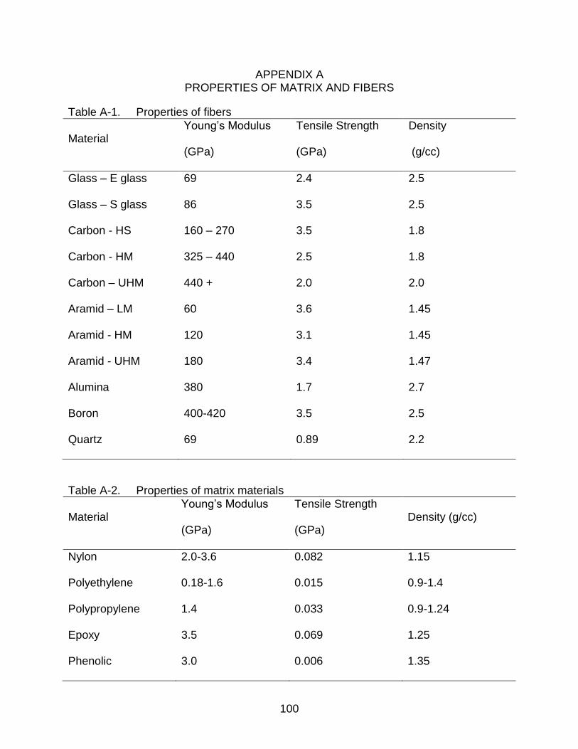
100
APPENDIX A PROPERTIES OF MATRIX AND FIBERS
Table A-1. Properties of fibers
Material Young’s Modulus
(GPa)
Tensile Strength
(GPa)
Density
(g/cc)
Glass – E glass 69 2.4 2.5
Glass – S glass 86 3.5 2.5
Carbon - HS 160 – 270 3.5 1.8
Carbon - HM 325 – 440 2.5 1.8
Carbon – UHM 440 + 2.0 2.0
Aramid – LM 60 3.6 1.45
Aramid - HM 120 3.1 1.45
Aramid - UHM 180 3.4 1.47
Alumina 380 1.7 2.7
Boron 400-420 3.5 2.5
Quartz 69 0.89 2.2
Table A-2. Properties of matrix materials
Material Young’s Modulus
(GPa)
Tensile Strength
(GPa) Density (g/cc)
Nylon 2.0-3.6 0.082 1.15
Polyethylene 0.18-1.6 0.015 0.9-1.4
Polypropylene 1.4 0.033 0.9-1.24
Epoxy 3.5 0.069 1.25
Phenolic 3.0 0.006 1.35

101
APPENDIX B MATERIAL PROPERTIES OF VARIOUS LAMINATES
Table B-1. Properties of various laminates
Material E1
(GPa)
E2
(GPa)
G12
(GPa)
ν12
(no units)
Density
(g/cc)
Carbon/PEEK
(unidirectional) 134 8.9 5.1 0.28 1.6
Carbon/Epoxy (Woven) 56.3 55.2 2.85 0.042 1.45
Carbon/Epoxy
(unidirectional) 300 6.5 5.0 0.23 1.59
E-Glass/Epoxy
(unidirectional) 39 8.6 3.8 0.28 2.10
E-Glass/Epoxy(woven) 25 25 4.0 0.20 1.90
S-Glass/Epoxy
(unidirectional) 43 8.9 4.5 0.27 2.00
S-Glass/Epoxy
(Woven) 29.7 29.7 5.3 0.17 2.20
Kevlar/Epoxy
(unidirectional) 87 5.5 2.2 0.34 1.38
Kevlar/Epoxy (Woven) 30 30 5.0 0.30 1.4
Boron/ Epoxy
(unidirectional) 200 15 5.0 0.23 2.00

102
LIST OF REFERENCES
[1] Jacob Fish and Ted Belytschko, A First Course in Finite Elements, JOHN WILEY & SONS LTD., 2007
[2] K.J. Bathe, Finite Element Procedures, PRENTICE HALL, 1996
[3] Christophe Dauxz, Nicolas Moes, John Dolbow,Natarajan Sukumar k and Ted Belytschko, Arbitrary branched and intersecting cracks with the extended finite element method, INTERNATIONAL JOURNAL FOR NUMERICAL METHODS IN ENGINEERING 2000; 48:1741-1760
[4] P. Lancaster and K. Salkauskas, Surfaces Generated by Moving Least Squares Methods, MATHEMATICS OF COMPUTATION, VOL. 37, NO. 155, July 1981
[5] Y.Y.Lu, T.Belytschko, L.Gu, A new implementation of Element Free Galerkin Method (EFGM), COMPUTER METHODS IN APPLIED MECHANICS AND ENGINEERING, 113, 1994, 397- 414
[6] Satya N. Atluri, The Meshless Local Petrov-Galerkin (MLPG)Method for Domain & BIE Discretizations, INTERNATIONAL WORKSHOP ON MESH-FREE METHODS, 2003
[7] Ashok V. Kumar and Jongho Lee, Step Function Representation of Solid Models and Application to Mesh-Free Engineering Analysis, ASME,128(1). Pp. 46-56.
[8] Ashok V. Kumar and Premdheepak S. Periyasamy, Mesh Independent Analysis of Shell-Like Structures, INTERNATIONAL JOURNAL FOR NUMERICAL METHODS AND ENGINEERING, 2011
[9] Ravi K. Burla and Ashok V. Kumar, Implicit boundary method for analysis using uniform B-spline basis and structured grid, INTERNATIONAL JOURNAL FOR NUMERICAL METHODS IN ENGINEERING, 2008
[10] Ashok V. Kumar, Ravi K. Burla, Sanjeev Padmanaban and Linxia Gu, Finite Element Analysis using Nonconforming Mesh, JOURNAL OF COMPUTING AND INFORMATION SCIENCE IN ENGINEERING, Sep. 2008
[11] E. Carrera, Theories and Finite Elements for Multilayered, Anisotropic Composite Plates and Shells, ARCHIVES IN COMPUTATIONAL METHODS IN ENGINEERING, VOL. 9, 2, 87-140, 2002
[12] Y.X. Zhang and C.H. Yang, Recent Developments in Finite Element Analysis for Laminated Composite Plates, COMPOSITE STRUCTURES, 88, 2009
[13] M. Nurhaniza, M.K.A. Ariffin, Aidy Ali, F. Mustapha and A. W. Noraini, Finite Element Analysis of Composite Materials for Aerospace Applications, 9TH NATIONAL SYMPOSIUM ON POLYMERIC MATERIALS, 2009
103
[14] P.F. Liu, J.Y. Zheng, Recent Developments on Damage Modeling and Finite Element Analysis for Composite Plates: A review, MATERIALS AND DESIGN, 2010
[15] J.N. Reddy, Bending of Laminated Anisotropic Shells by a Shear Deformable Finite Element, FIBER SCIENCE AND TECHNOLOGY 17, 1982
[16] R.J. Razzaq, A. El-Zafrany, Non – linear stress analysis of composite layered plates and shells using a mesh reduction method, ENGINEERING ANALYSIS WITH BOUNDARY ELEMENTS 29, 2005
[17] J. Sladek, V. Sladek and S.N. Atluri, Meshless Local Petrov-Galerkin (MLPG) Method in Anisotropic Elasticity, COMPUTER MODELING IN ENGINEERING AND SCIENCES (CMES) VOL.6, NO. 5, 2004
[18] J. Belinha and L.M.J.S. Dinis, Non- linear analysis of plates and laminates using the Element Free Galerkin Method (EFGM), COMPOSITE STRUCTURES 78, 2007
[19] B.N. Pandya and T. Kant, Finite Element Analysis of Composite Plates using a High-order displacement model, COMPOSITES SCIENCE AND TECHNOLOGY 32, 1988
[20] J.R. Xiao, R.C. Batra, D.F. Gilhooley, J.W. Gillespie Jr., M.A. McCarthy, Analysis of thick plates by using a Higher Order Shear and Normal Deformable Plate Theory (HOSNDPT) and a Meshless Local Petrov-Galerkin (MLPG) Method with Radial Basis Functions, COMPUTER METHODS IN APPLIED MECHANICS AND ENGINEERING 196, 2007
[21] Zafer Gurdal, Rapheal T. Haftka and Prabhat Hajela, Design and Optimization of Laminated Composite Materials, JOHN WILEY & SONS LTD., 1999
[22] Robert M. Jones, Mechanics of Composite Materials, TAYLOR & FRANCIS GROUP, 1999
[23] J.N. Reddy, Mechanics of Laminated Composite Plates and Shells: Theory and Analysis, CRC PRESS, 1997
[24] Autar K. Kaw, Mechanics of Composite Materials, TAYLOR & FRANCIS GROUP, 2006
[25] Ronald F. Gibson, Principles of Composite Material Mechanics, CRC PRESS, 2007
[26] T. Belytschko, Y. Krongauz, D. Organ, M. Fleming, P. Krysl, Meshless Methods: An overview and recent developments, COMPUTER METHODS IN APPLIED MECHANICS AND ENGINEERING, 1996

104
[27] J.J.Monaghan, An Introduction to SPH, COMPUTER PHYSICS COMMUNICATIONS 48 (1988) 89-96
[28] Kantorovich LV, Krylov VI, Approximate Methods for Higher Analysis, INTERSCIENCE PUBLISHERS INC., 1958
[29] V.Shapiro, I.Tsukanov, Meshfree simulation of deforming domains, COMPUTER AIDED DESIGN 31 (1999) 459–471
[30] Lidia Kurpa, Galina Pilgun, Eduard Ventsel, Application of the R-function method to nonlinear vibrations of thin plates of arbitrary shape, JOURNAL OF SOUND AND VIBRATION 284 (2005) 379–392
[31] Tae-Kyoung Uhm and Sung-Kie Youn, T-Spline Finite Element Method for the analysis of shell structures, INTERNATIONAL JOURNAL FOR NUMERICAL METHODS IN ENGINEERING, June 2009
[32] James D. Lee, Three Dimensional Finite Element Analysis of Layered Fiber-reinforced Composite Materials, COMPUTERS AND STRUCTURES, 1980
[33] Tarapada Roy, P.Manikandan, Debabrata Chakraborty, Improved Shell Finite Element for Piezothermoelastic Analysis of Smart Fiber Reinforced Composite Structures, FINITE ELEMENTS IN ANALYSIS AND DESIGN, 2010
[34] Y. Basar, M. Itskov, A. Eckstein, Composite laminates: nonlinear interlaminar stress analysis by multi-layer shell elements, COMPUTER METHODS IN APPLIED MECHANICS AND ENGINEERING, 2000
[35] R.L. Spilker, S.C. Chou, O. Orringer, Alternate Hybrid-Stress Elements for Analysis of Multilayered Composite Plates, JOURNAL OF COMPOSITE MATERIALS, 1977
[36] Juan Miquel, Salvador Botello and Eugenio Onate, A finite element formulation for analysis of composite laminate shells, INTERNATIONAL CENTER FOR NUMERICAL METHODS IN ENGINEERING
[37] Sun C.T., Mechanics of Aircraft Structures, JOHN WILEY & SONS LTD., 1998
[38] O.O. Ochoa and J.N. Reddy, Finite Element Analysis of Composite Laminates, KLUWER ACADEMIC PUBLISHERS, 1992
[39] Premdheepak Salem Periyasamy, Finite Element Analysis of shell like structures using Implicit Boundary Method, UNIVERSITY OF FLORIDA, 2012
[40] Hailong Chen, Mixed formulation using Implicit Boundary Finite Element Method, UNIVERSITY OF FLORIDA, 2012
105
BIOGRAPHICAL SKETCH
Vignesh Solai Rameshbabu was born and brought up in a small industrial town
called Neyveli, in the state of Tamil Nadu, India. He did his high school in Jawahar
Higher Secondary School in Neyveli and graduated in 2005. Then, he joined Hindustan
College of Engineering, Anna University in the year of 2005 and graduated with a
bachelor’s degree in aeronautical engineering with the specialization in Aircraft
Structures, Aerodynamics and Aircraft Propulsion in 2009. Meanwhile, he gained some
industrial experience by undergoing a 1 month industrial training in June 2007 at the
Ground-Test Centre, Rotary-Wing Research and Development Centre, Hindustan
Aeronautics Ltd, Bangalore, India. Then, he worked as a Design Engineer in the Design
Department, in a manufacturing industry called DMW CNC Solutions Pvt. Ltd., which is
located in a small town called Perundurai, Tamil Nadu, India. Then, he received a
master’s degree in aerospace engineering in the summer of 2012 from the University of
Florida, Gainesville, Florida, USA. His areas of specialization include Finite Element
Method, Aerospace Composites, Computational Methods in Design and Manufacturing
and developing softwares used in Mechanical/Aerospace/Automotive/Civil Engineering
using Object Orientation Programming Techniques.