c 2015 by vivek kale. all rights reserved
TRANSCRIPT

c© 2015 by Vivek Kale. All rights reserved.
LOW-OVERHEAD SCHEDULING FOR IMPROVINGPERFORMANCE OF SCIENTIFIC APPLICATIONS
BY
VIVEK KALE
DISSERTATION
Submitted in partial fulfillment of the requirementsfor the degree of Doctor of Philosophy in Computer Science
in the Graduate College of theUniversity of Illinois at Urbana-Champaign, 2015
Urbana, Illinois
Doctoral Committee:
Professor William D. Gropp, ChairDr. Bronis R. DeSupinski, Lawrence Livermore National LaboratoryProfessor Maria GarzaranProfessor David Padua

Abstract
Application performance can degrade significantly due to node-local load
imbalances during application execution on a large number of SMP nodes.
These imbalances can arise from the machine, operating system, or the ap-
plication itself. Although dynamic load balancing within a node can mit-
igate imbalances, such load balancing is challenging because of its impact
to data movement and synchronization overhead. We developed a series of
scheduling strategies that mitigate imbalances without incurring high over-
head. Our strategies provide performance gains for various HPC codes, and
perform better than widely known scheduling strategies such as OpenMP
guided scheduling. Our scheme and methodology allows for scaling appli-
cations to next-generation clusters of SMPs with minimal application pro-
grammer intervention. We expect these techniques to be increasingly useful
for future machines approaching exascale.
ii
Acknowledgments
This work would not be possible without the help of many people. First,
thanks to my advisor, Professor Bill Gropp, who provided me with several
revisions to my thesis, several technical suggestions (including code develop-
ment) throughout, and an initial and continual drive to learn new concepts
and to solve challenging problems through a PhD. Additionally, I would like
thank Professor Micheal Heath for helping to make the theoretical analysis
part of this work more formal and systematic. Thanks to Simplice Donfack
for his collaboration and support of the work on applying hybrid static/dy-
namic scheduling to dense matrix factorizations, and to Laura Grigori for
overseeing a large portion of this work. Thanks also to Jim Demmel for
discussing my work in the context of dense matrix factorizations, and for
providing impetus for detailed investigation locality-based optimizations for
dense matrix factorizations. I would like to especially thank Todd Gamblin
for providing support for the software system that increased the applica-
bility of this work and grew this work further, and to Bronis de Supinski
for providing strategic research direction for runtime optimizations of our
low-overhead scheduling techniques. Additionally, I’d like to thank Steve
Langer who posed important questions to think about from an application
programmer’s point of view. I would also like to thank Martin Schulz for
providing input on performance profiling, along with the LC division at
Lawrence Livermore National Laboratory for providing technical support
on the clusters at LLNL. I would also like to thank Torsten Hoefler for
his input on performance modeling and theoretical analysis of low-overhead
scheduling strategies. Thanks to my committee members David Padua and
Maria Garzaran for their generous feedback and input throughout the dis-
sertation process. Thanks to my labmates from the Scientific Computing
Group at the University of Illinois at Urbana-Champaign for their feedback
in practice presentations. Finally, this work would not be possible without
the unconditional support and caring of family and friends throughout the
PhD and the dissertation process.
iii

Table of Contents
List of Tables . . . . . . . . . . . . . . . . . . . . . . . . . . . . vii
List of Figures . . . . . . . . . . . . . . . . . . . . . . . . . . . . viii
List of Abbreviations . . . . . . . . . . . . . . . . . . . . . . . xii
List of Symbols . . . . . . . . . . . . . . . . . . . . . . . . . . . xiii
Chapter 1 Introduction and Motivation . . . . . . . . . . . 11.1 Cache Miss Calculations . . . . . . . . . . . . . . . . . . . . . 101.2 Contributions . . . . . . . . . . . . . . . . . . . . . . . . . . . 121.3 Thesis Outline . . . . . . . . . . . . . . . . . . . . . . . . . . 13
Chapter 2 Hybrid Static/Dynamic Scheduling . . . . . . . 142.1 Basic Mixed Static/Dynamic Scheduling Technique . . . . . . 142.2 Results for Barnes-Hut and NAS LU with Mixed Static/Dy-
namic Scheduling . . . . . . . . . . . . . . . . . . . . . . . . . 172.2.1 An Empirical Method for Finding the Best Static Frac-
tion . . . . . . . . . . . . . . . . . . . . . . . . . . . . 182.3 Study with MPI Code And Outer Iteration Locality . . . . . 22
2.3.1 A Scheduler for Outer Iteration Locality . . . . . . . . 222.3.2 MPI Regular Mesh Computation . . . . . . . . . . . . 232.3.3 Tuning Tasklet Granularity for Reduced Thread Idle
Time . . . . . . . . . . . . . . . . . . . . . . . . . . . . 292.3.4 Using Our Technique to Improve Scalability . . . . . . 31
2.4 Results for Numerical Linear Algebra . . . . . . . . . . . . . . 352.5 Conclusions . . . . . . . . . . . . . . . . . . . . . . . . . . . . 38
Chapter 3 Weighted Hybrid Scheduling . . . . . . . . . . . 393.1 Platforms Considered . . . . . . . . . . . . . . . . . . . . . . 403.2 Scheduling Techniques . . . . . . . . . . . . . . . . . . . . . . 42
3.2.1 Allocating Iterations Based on Weights . . . . . . . . 443.3 Results for Weighted Hybrid Scheduling . . . . . . . . . . . . 45
3.3.1 Weighted Scheduling . . . . . . . . . . . . . . . . . . . 473.3.2 Micro-scheduling . . . . . . . . . . . . . . . . . . . . . 483.3.3 Weighted micro-scheduling . . . . . . . . . . . . . . . 493.3.4 Experimentation with Varying Problem Sizes . . . . . 503.3.5 Impact of Memory Accessed per Time Step . . . . . . 50
iv
3.4 Discussion . . . . . . . . . . . . . . . . . . . . . . . . . . . . . 50
Chapter 4 Slack-Conscious Hybrid Static/Dynamic Schedul-ing . . . . . . . . . . . . . . . . . . . . . . . . . . . . . . . . . 534.1 Performance Perturbances . . . . . . . . . . . . . . . . . . . . 544.2 Model-Based Determination of Minimal Dynamic Fraction . . 55
4.2.1 Using a Model for Hybrid Scheduling . . . . . . . . . . 554.3 Communication Deadlines and Slack . . . . . . . . . . . . . . 57
4.3.1 Characterizing Slack . . . . . . . . . . . . . . . . . . . 584.3.2 Existing Thread Scheduling Policies In the Context of
Slack . . . . . . . . . . . . . . . . . . . . . . . . . . . . 594.4 Extending the Model to Incorporate Slack . . . . . . . . . . . 614.5 Slack-Conscious Hybrid Static/Dynamic Scheduling . . . . . 63
4.5.1 Automatic Compiler Transformation . . . . . . . . . . 654.5.2 Runtime Parameter Estimation . . . . . . . . . . . . . 66
4.6 Experimental Evaluation . . . . . . . . . . . . . . . . . . . . . 684.6.1 System-Specific Noise Signatures . . . . . . . . . . . . 694.6.2 Slack Prediction Accuracy and Overhead . . . . . . . 694.6.3 Comparing Slack-conscious Scheduling with Best Static
Fraction . . . . . . . . . . . . . . . . . . . . . . . . . . 704.6.4 Implementation Strategy Assessment . . . . . . . . . . 714.6.5 Overall Application Performance . . . . . . . . . . . . 74
4.7 Conclusion . . . . . . . . . . . . . . . . . . . . . . . . . . . . 76
Chapter 5 Spatial Locality in Dynamically Assigned Itera-tions . . . . . . . . . . . . . . . . . . . . . . . . . . . . . . . . 775.1 Problem Statement . . . . . . . . . . . . . . . . . . . . . . . . 785.2 Scheduling Strategy . . . . . . . . . . . . . . . . . . . . . . . 79
5.2.1 Modifications to Allocation of Iterations . . . . . . . . 795.2.2 Choosing the Thread From Which to Steal . . . . . . 80
5.3 Implementation . . . . . . . . . . . . . . . . . . . . . . . . . . 815.3.1 Framework and Usage . . . . . . . . . . . . . . . . . . 825.3.2 Implementation of Locality Optimized Static/Dynamic
Scheduling . . . . . . . . . . . . . . . . . . . . . . . . 825.4 Experimental Evaluation . . . . . . . . . . . . . . . . . . . . . 83
5.4.1 Implementation Overhead . . . . . . . . . . . . . . . . 845.4.2 Application Performance . . . . . . . . . . . . . . . . . 85
5.5 Conclusion . . . . . . . . . . . . . . . . . . . . . . . . . . . . 87
Chapter 6 Composing Multiple Scheduling Strategies . . . 906.1 Scheduling Strategies Overview . . . . . . . . . . . . . . . . . 906.2 Techniques for Composing Schedulers . . . . . . . . . . . . . 92
6.2.1 hybSched . . . . . . . . . . . . . . . . . . . . . . . . . 936.2.2 tunedSched . . . . . . . . . . . . . . . . . . . . . . . . 936.2.3 NoiseModelSched . . . . . . . . . . . . . . . . . . . . . 946.2.4 AppModelSched . . . . . . . . . . . . . . . . . . . . . 946.2.5 modelSched . . . . . . . . . . . . . . . . . . . . . . . . 956.2.6 uSched . . . . . . . . . . . . . . . . . . . . . . . . . . . 95
v

6.2.7 slackSched . . . . . . . . . . . . . . . . . . . . . . . . . 956.2.8 vSched . . . . . . . . . . . . . . . . . . . . . . . . . . . 966.2.9 ComboSched . . . . . . . . . . . . . . . . . . . . . . . 966.2.10 Code Transformation . . . . . . . . . . . . . . . . . . . 97
6.3 Results . . . . . . . . . . . . . . . . . . . . . . . . . . . . . . . 986.3.1 Application Programmer Effort . . . . . . . . . . . . . 102
6.4 Relevance to Future Architectures . . . . . . . . . . . . . . . 102
Chapter 7 Related Work . . . . . . . . . . . . . . . . . . . . 105
Chapter 8 Conclusions . . . . . . . . . . . . . . . . . . . . . . 110
References . . . . . . . . . . . . . . . . . . . . . . . . . . . . . . 113
vi
List of Tables
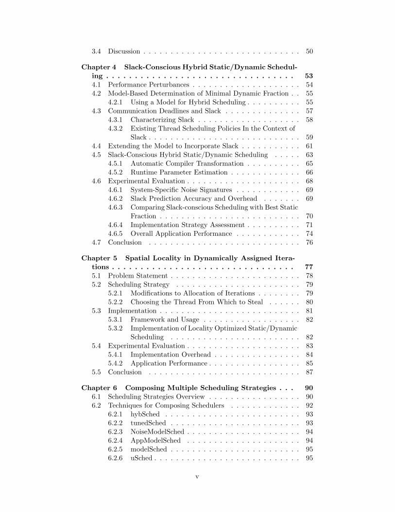
1.1 Standard load imbalance metric across all cores of multiplenodes of Cab. . . . . . . . . . . . . . . . . . . . . . . . . . . . 4
1.2 Standard load imbalance metric taken across nodes (withineach node, load is summed across cores) for the above N-bodycomputation run on Cab, added to the rightmost column. . . 4
2.1 Table showing performance gains over OpenMP static forNAS benchmarks with besf on cab. . . . . . . . . . . . . . . . 22
2.2 Table showing performance gains over OpenMP static forNAS benchmarks with besf on rzuseq. . . . . . . . . . . . . . 22
4.1 Overview of all model parameters. . . . . . . . . . . . . . . . 564.2 Slack statistics (in µs) across MPI processes. . . . . . . . . . 584.3 Overview of all model parameters. . . . . . . . . . . . . . . . 62
5.1 Overheads of our scheduling runtime shown as the percentagedifference between our library’s static scheduling and OpenMPstatic scheduling. . . . . . . . . . . . . . . . . . . . . . . . . . 84
5.2 Barnes-Hut standard deviations of execution times across 15trials, where a trial is a job submission of the code. . . . . . . 88
vii
List of Figures
1.1 Schematics of application timelines showing how impact ofnoise can be mitigated by idealized within-node work re-distribution. . . . . . . . . . . . . . . . . . . . . . . . . . . . . 3
1.2 A modeled application timeline having load imbalance onsome particular node through a re-distribution of work acrosscores within a node provides improved performance. . . . . . 3
1.3 Calculation of the total overhead of thread idle time for anMPI+OpenMP code. . . . . . . . . . . . . . . . . . . . . . . . 7
1.4 Breakdown of execution time for a load imbalanced code (left)and a load balanced code (right) on cab, shown for the threeavailable OpenMP scheduling strategies. . . . . . . . . . . . . 7
1.5 Breakdown of time. Synchronization overheads are shown ingreen. . . . . . . . . . . . . . . . . . . . . . . . . . . . . . . . 8
1.6 Cache misses with L2 misses on top and L3 on bottom, fordifferent OpenMP scheduling strategies. . . . . . . . . . . . . 9
2.1 Impact of performance irregularities for static scheduling. . . 152.2 Dynamic scheduling of one invocation of a threaded compu-
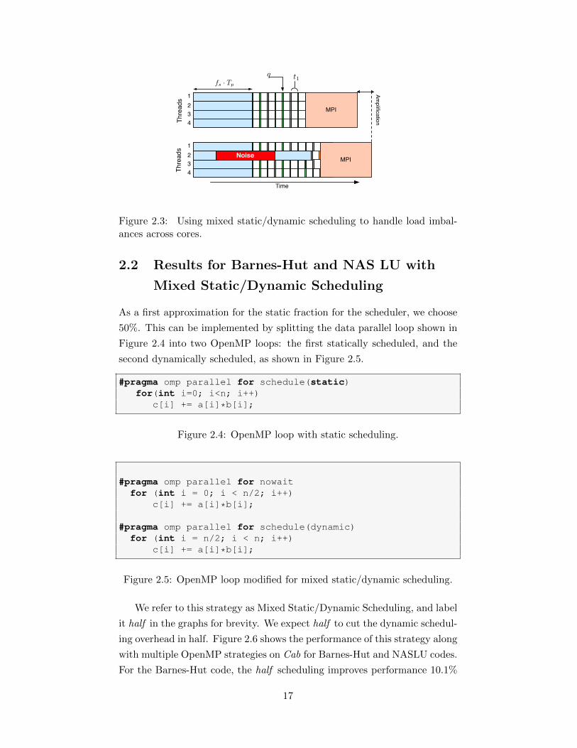
tation region on an arbitrary MPI process. . . . . . . . . . . . 162.3 Using mixed static/dynamic scheduling to handle load imbal-
ances across cores. . . . . . . . . . . . . . . . . . . . . . . . . 172.4 OpenMP loop with static scheduling. . . . . . . . . . . . . . . 172.5 OpenMP loop modified for mixed static/dynamic scheduling. 172.6 Set fs = 0.5: In half, threads do the first half of their iterations
statically. See rightmost bar in the bar graph. . . . . . . . . . 182.7 OpenMP statically scheduled loop transformed for hybrid
static/dynamic scheduling. . . . . . . . . . . . . . . . . . . . . 192.8 Performance for different static fractions when using hybrid
static/dynamic scheduling for Barnes-Hut. . . . . . . . . . . . 202.9 Performance for different static fractions when using hybrid
static/dynamic scheduling for NAS LU. . . . . . . . . . . . . 202.10 Execution time breakdown with the besf strategy added on
the rightmost bar. . . . . . . . . . . . . . . . . . . . . . . . . 212.11 L2 cache misses shown in the top graphs; L3 in the bottom.
The best static fraction strategy is added on the rightmost bar. 212.12 3D stencil domain decomposition across MPI processes. . . . 24
viii
2.13 3D stencil domain decomposition across MPI processes, alongwith thread partitioning of work within each MPI process. . . 25
2.14 Histograms for static scheduling on 1 node, showing bi-modaldistribution. . . . . . . . . . . . . . . . . . . . . . . . . . . . . 25
2.15 3D stencil decomposition with a dynamic scheduling strategyapplied. . . . . . . . . . . . . . . . . . . . . . . . . . . . . . . 26
2.16 3D stencil decomposition with a locality-aware schedulingstrategy applied. . . . . . . . . . . . . . . . . . . . . . . . . . 26
2.17 3D stencil decomposition with our mixed static/dynamic schedul-ing strategy applied. . . . . . . . . . . . . . . . . . . . . . . . 27
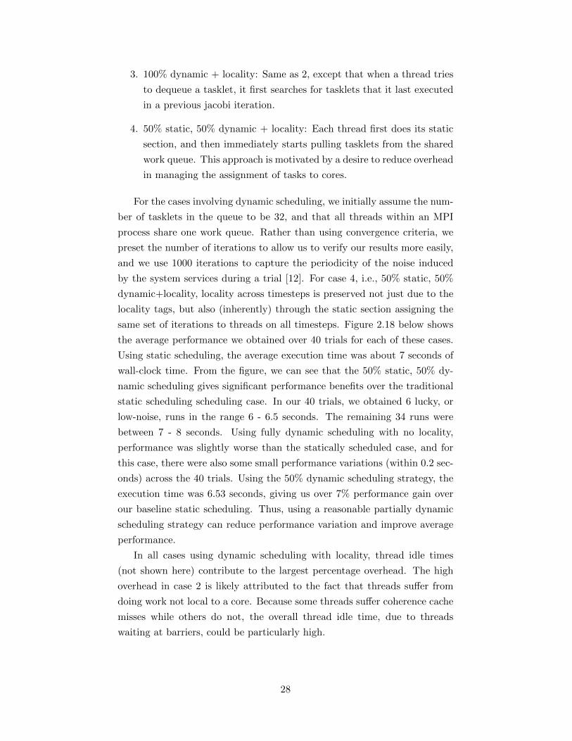
2.18 Performance for different scheduling strategies on a singlenode of IBM Power5+ cluster of SMPs. . . . . . . . . . . . . 29
2.19 Performance for scheduling with different numbers of planesper tasklet. . . . . . . . . . . . . . . . . . . . . . . . . . . . . 30
2.20 Iteration timing histograms of 3D regular mesh run on singlenode of IBM Power 5+ cluster, where each histogram corre-sponds to a different scheduling strategy applied to the 3Dregular mesh. . . . . . . . . . . . . . . . . . . . . . . . . . . 31
2.21 Scaling behavior of different scheduling strategies. . . . . . . 332.22 Performance consistency is maintained for mixed static/dy-
namic scheduling for 1 nodes. . . . . . . . . . . . . . . . . . . 332.23 Performance consistency is maintained for mixed static/dy-
namic scheduling for 2 nodes. . . . . . . . . . . . . . . . . . . 342.24 Performance consistency is maintained for hybrid static/dy-
namic scheduling for 16 nodes. . . . . . . . . . . . . . . . . . 342.25 Performance consistency is maintained for hybrid static/dy-
namic scheduling for 64 nodes. . . . . . . . . . . . . . . . . . 352.26 Performance of Hybrid Static/Dynamic Scheduled CALU, MKL
and PLASMA on the 16-core Intel machine. . . . . . . . . . 372.27 Performance of Hybrid Static/Dynamic Scheduled CALU, MKL
and PLASMA on the 48-core AMD Opteron machine. . . . . 372.28 Performance variation of CALU on an AMD Opteron 24-core
node of a cluster. . . . . . . . . . . . . . . . . . . . . . . . . . 38
3.1 System noise plotted against all ranks for a 100 node run forJaguar and Ranger. . . . . . . . . . . . . . . . . . . . . . . . 40
3.2 Histograms for the execution time of a sequential computationperformed to record noise events on Jaguar (left) and Ranger(right). The labels on the x-axis are bin-numbers. . . . . . . . 41
3.3 MPI domain decomposition used for the 3D Stencil code. . . 453.4 Hybrid MPI+pthreads domain decomposition with micro-scheduling
used for the 3D Stencil code. The dynamic fraction is denotedby fd. . . . . . . . . . . . . . . . . . . . . . . . . . . . . . . . 46
ix

3.5 Hybrid MPI+pthreads domain decomposition used with weightedstatic and dynamic micro-scheduling for the three-dimensional7-point stencil computation. The dynamic fraction is denotedby fd, and the weight of thread 1, as shown in this diagram,is denoted by w1. . . . . . . . . . . . . . . . . . . . . . . . . . 46
3.6 Performance of the stencil computation on Jaguar for variousscheduling techniques. . . . . . . . . . . . . . . . . . . . . . . 47
3.7 Performance of the stencil computation on Ranger for variousscheduling techniques. . . . . . . . . . . . . . . . . . . . . . . 48
3.8 Impact of problem size on Jaguar for 3D Stencil with differentload balancing strategies. . . . . . . . . . . . . . . . . . . . . 51
3.9 Impact of problem size on Ranger for 3D Stencil with differentload balancing strategies. . . . . . . . . . . . . . . . . . . . . 52
4.1 Slack in a binomial broadcast tree with four processes. . . . 594.2 Impact of performance irregularities for static scheduling, with
slack factor added. . . . . . . . . . . . . . . . . . . . . . . . . 604.3 Resilience to performance irregularities with dynamic schedul-
ing, with slack factor added. . . . . . . . . . . . . . . . . . . . 604.4 Hybrid Scheduling for a threaded computation region, with
the slack factor added. . . . . . . . . . . . . . . . . . . . . . . 614.5 Runtime framework with our contributions in grey. . . . . . 644.6 Transformation of an OpenMP loop to use our approach. . . 654.7 Scaling PF3D on a Intel Westmere 12-core cluster. . . . . . . 684.8 Noise signatures for our test systems. . . . . . . . . . . . . . . 694.9 Average error of runtime’s slack prediction across all MPI
processes, for different applications. . . . . . . . . . . . . . . . 704.10 Average overhead of implementation of slack prediction li-
brary function across all MPI processes for different applica-tions. . . . . . . . . . . . . . . . . . . . . . . . . . . . . . . . . 70
4.11 Comparison of our scheduling technique with using the beststatic fraction on Cab. . . . . . . . . . . . . . . . . . . . . . . 72
4.12 Performance for different scheduling strategies shown as per-centage speedup over OpenMP static scheduling. . . . . . . . 73
4.13 Overheads for different scheduling strategies as a percent oftotal runtime. Dequeue overhead is hashed, and thread idletime is solid. . . . . . . . . . . . . . . . . . . . . . . . . . . . 73
4.14 Scaling runs of all five applications. . . . . . . . . . . . . . . . 744.15 Scalability of PF3D with different schedulers on cab. . . . . . 75
5.1 Allocation of iterations to threads for Hybrid Static/DynamicScheduling. . . . . . . . . . . . . . . . . . . . . . . . . . . . . 80
5.2 Allocation of loop iterations to threads for Staggered HybridStatic/Dynamic Scheduling. . . . . . . . . . . . . . . . . . . . 80
5.3 Framework for our modified portion of the thread library. . . 815.4 Transformation of a loop to use our approach. . . . . . . . . . 835.5 Barnes-Hut code main modification using Slack-Conscious
Hybrid Static/Dynamic scheduling. . . . . . . . . . . . . . . . 86
x

5.6 Improvement obtained over OpenMP static scheduling for dif-ferent scheduling strategies applied to Barnes-Hut, shown for4 of 16 cores of Cab. . . . . . . . . . . . . . . . . . . . . . . . 87
5.7 Improvement obtained over OpenMP static scheduling for dif-ferent scheduling strategies applied to Barnes-Hut, shown for8 of 16 cores of Cab. . . . . . . . . . . . . . . . . . . . . . . . 88
5.8 Improvement obtained over OpenMP static scheduling fordifferent scheduling strategies applied to Barnes-Hut, for 16cores of Cab. . . . . . . . . . . . . . . . . . . . . . . . . . . . 88
5.9 Improvement obtained over OpenMP static scheduling for dif-ferent scheduling strategies applied to a stencil code, runningon 16 cores of Cab. . . . . . . . . . . . . . . . . . . . . . . . . 89
6.1 Composition of 8 schedulers that make comboSched. . . . . . 936.2 Original code with OpenMP loop. . . . . . . . . . . . . . . . 976.3 Code transformed to use composed scheduler. . . . . . . . . . 996.4 Rebound(N-body): Performance improvement obtained over
OpenMP static scheduling. . . . . . . . . . . . . . . . . . . . 1006.5 miniFE (finite element): Performance improvement obtained
over OpenMP static scheduling. . . . . . . . . . . . . . . . . 1016.6 SNAP (regular mesh): Performance improvement obtained
over OpenMP static scheduling. . . . . . . . . . . . . . . . . 1026.7 Total lines of code changed and average lines of code changed per
threaded computation region for the Rebound N-body, CORAL
SNAP and CORAL miniFE. . . . . . . . . . . . . . . . . . . . . 102
xi

List of Abbreviations
MPI Message Passing Interface
HPC High Performance Computing
LDB Load Balancer
static OpenMP Static scheduling
dynamic OpenMP Dynamic scheduling
guided OpenMP Guided scheduling
half Basic Hybrid Static/Dynamic Scheduling with 50% staticfraction
besf Basic Hybrid Static/Dynamic Scheduling
wSched Weighted Factoring for Persistent Load Imbalances
uWldb Weighted Hybrid Static/Dynamic Scheduling
sSch Slack-Conscious Mixed Static/Dynamic Scheduling
sds Staggered Static/Dynamic Scheduling.
combo Example scheduler composition.
xii

List of Symbols
τ Time taken to complete the computational work of a dynamicallyscheduled task.
δ Duration of excess work or idle time.
d Number of tasks to be dynamically scheduled in a threaded com-putation region.
N Number of loop iterations in a threaded computation region.
t1 Length of time for a single loop iteration.
Tp Time needed for computational work on p cores of a cluster’smulti-core node.
Si Slack duration on process i.
xiii
Chapter 1
Introduction and Motivation
As applications become more sophisticated and architectures become more
complex, a supercomputer may not be utilized to its peak performance [9,15,
29, 78]. Specifically, during application execution on a large number of pro-
cessors, load imbalance can cause parallel efficiency of scientific applications
to deteriorate with an increasing number of processors.
We focus on iterative MPI computations. Iterations may correspond to
timesteps, numerical iterations, or both. In each iteration, steps involve
synchronization across nodes, such as global reductions or near-neighbor
communications. Broadly, applications with these characteristics can be
called bulk-synchronous or loosely-synchronous.
Consider the kinds of load imbalances that arise in this context. Some
imbalances arise somewhat randomly across individual cores. We can think
of these as transient and uncoordinated imbalances. Examples of these
types of imbalances are small, transient performance perturbances caused
by time-shared operating system daemons, correctable hardware errors, vari-
able memory access latencies, software floating-point exception handling,
and dynamic CPU frequency management for power conservation [12, 61,
65, 70]. For brevity, we will call these variations noise, while noting that it
is a generalization of the conventional definition of noise, which is typically
associated with operating system daemons [12,52,72].
The other category of imbalances arises from load variability. Here, code
executing on different threads takes different amounts of time, and so ar-
rives at synchronization points at different times during each step. Many
situations in which this happens involve persistent load imbalances. Persis-
tent load imbalances have a (relatively) fixed pattern of load distributions
across cores, over iterations of an application. The balance may shift some-
what across iterations, slowly, but the broad pattern remains similar. A
major source of persistent load imbalances are the applications themselves.
For example, application load imbalances exist in sparse matrix-vector mul-
tiplication used in quantum chromodynamics simulations [74] and N-body
1
force calculations used in molecular dynamic simulations [73]. Addition-
ally, static variations in speeds of different cores may lead to persistent
imbalances as well. Load variability also includes situations that are non-
persistent imbalances. Here, the load variation significantly changes after
every few iterations, such as in the case of adaptive mesh refinement [37].
A potential method for mitigating both of these categories of load im-
balances is suggested by the fact that the number of cores per node is large
and is steadily increasing over time [78]. Many machines with conventional
processors have 32-64 cores per node, e.g., Cray’s Titan, or IBM’s Mira
(BG/Q) [1,2]. Future versions of many-core processors, such as Intel’s Xeon
Phi, are likely to have several hundred cores per node [87]. It has been
predicted that for an exascale machine, the number of nodes will not be
much larger than today’s petascale machines, but the number of cores per
node will be substantially larger [9]. The existence of large numbers of cores
within each node can be potentially utilized to reduce global load imbal-
ance by dynamically equalizing the load within each node. This is the key
approach that provides the context for this thesis.
The schematics in Figures 1.1 and 1.2 illustrate why our key approach
mentioned above is potentially attractive. In these figures, the x-axis is time,
and the y-axis is core number. A horizontal line represents the timeline
of a core. A white space in the core’s timeline represents the core’s idle
time. Consider the effects of system noise on overall performance, as shown
in Figure 1.1a. On each timestep, a core on a different node experiences
noise, given a system with a sufficiently large number of nodes. While
on some iterations, no node may experience noise, and on other iterations
multiple nodes might experience noise, the essential argument we are making
is still valid. Even though the noise on any given core is rare and would
not impact sequential computations significantly, the MPI synchronization
between computations slows down the parallel program significantly. Our
approach is illustrated by Figure 1.2b. If the load on the affected core can
be re-distributed to the remaining cores within that node without much
overhead, the overall impact of noise can be significantly reduced.
The schematic shown in Figure 1.2 applies for application-induced load
imbalance, which is typically persistent. The performance is affected by the
most heavily loaded core, as before. Again, if we could re-distribute the load
within each node equally, the performance would be substantially improved.
We make note that the indent on the node second to the bottom is due to
differences in load across nodes, and handling this problem is complementary
to this work. This re-distribution helps even for load variability that is not
2

persistent.
Node
(a) Noise occuring on different nodes in different iterationsdelays every iteration.
Node%
(b) Execution times are signifi-cantly reduced, if we assume loadcan be perfectly re-distributedwithin each node.
Figure 1.1: Schematics of application timelines showing how impact of noisecan be mitigated by idealized within-node work re-distribution.
(a) A modeled application timeline havingpersistent load imbalance across cores duringexecution.
(b) A modeled applica-tion timeline with workre-distributed across cores, toreduce load imbalance.
Figure 1.2: A modeled application timeline having load imbalance on someparticular node through a re-distribution of work across cores within a nodeprovides improved performance.
As a concrete example, consider the performance data shown in Table 1.2
for an N-body computation (a galaxy simulation) on a cluster named cab.
Cab is an Intel Xeon Cluster with 16 cores per node. The table shows load
imbalance during the application execution across all cores, in the form of
the ratio of the load on the heaviest loaded core to the average load per
core. This ratio captures the impact of load imbalance on execution time.
As expected, the load imbalance increases as the number of cores increases
in this strong scaling experiment.
To see how the above idealized approach will work for this example, we
3
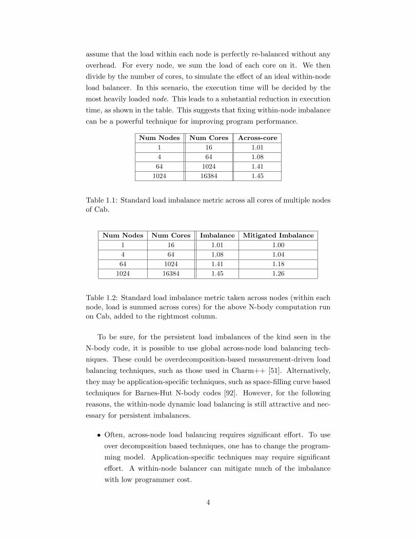
assume that the load within each node is perfectly re-balanced without any
overhead. For every node, we sum the load of each core on it. We then
divide by the number of cores, to simulate the effect of an ideal within-node
load balancer. In this scenario, the execution time will be decided by the
most heavily loaded node. This leads to a substantial reduction in execution
time, as shown in the table. This suggests that fixing within-node imbalance
can be a powerful technique for improving program performance.
Num Nodes Num Cores Across-core
1 16 1.01
4 64 1.08
64 1024 1.41
1024 16384 1.45
Table 1.1: Standard load imbalance metric across all cores of multiple nodesof Cab.
Num Nodes Num Cores Imbalance Mitigated Imbalance
1 16 1.01 1.00
4 64 1.08 1.04
64 1024 1.41 1.18
1024 16384 1.45 1.26
Table 1.2: Standard load imbalance metric taken across nodes (within eachnode, load is summed across cores) for the above N-body computation runon Cab, added to the rightmost column.
To be sure, for the persistent load imbalances of the kind seen in the
N-body code, it is possible to use global across-node load balancing tech-
niques. These could be overdecomposition-based measurement-driven load
balancing techniques, such as those used in Charm++ [51]. Alternatively,
they may be application-specific techniques, such as space-filling curve based
techniques for Barnes-Hut N-body codes [92]. However, for the following
reasons, the within-node dynamic load balancing is still attractive and nec-
essary for persistent imbalances.
• Often, across-node load balancing requires significant effort. To use
over decomposition based techniques, one has to change the program-
ming model. Application-specific techniques may require significant
effort. A within-node balancer can mitigate much of the imbalance
with low programmer cost.
4
• Even if global load balancing is used, a significant residual imbalance
remains because of imperfections in accurate predictions of load and
imperfections in load balancing algorithms themselves.
• Global load balancers can be faster if they focus on partitioning work
to the nodes (which are much smaller in number, compared with the
number of cores), leaving the within-node imbalance for a within-node
balancer.
• Often, applications with persistence still are not exactly repeating their
behavior every time step. As particles move in N-body codes, for
example, the load shifts slowly. This creates quasi-transient imbalance.
• Applications codes such as Adaptive Mesh Refinement, e.g., SAM-
RAI [37] or Shewchuck’s triangulation programs [83], change behavior
quickly as refinements and coarsenings are applied. A node may be a
sufficiently large unit that these effects are neutralized, but work allo-
cation to cores within a node must be changed after every refinement
or coarsening.
Utilizing multiple cores to dynamically balance load within each node
can be an effective technique for mitigating global load imbalance, without
undue burden on the programmer. Although the potential of this idea of
mitigating global load imbalance by dynamic load balancing within each
node is attractive, its utility critically depends on whether the dynamic
load balancing can be done effectively, and with low-overhead. Note that
we assumed an idealized, perfect load re-distribution in the example and
schematic above. The dominant methods for doing such load balancing, with
minimal programming effort for the application programmer, are provided
by OpenMP. However, as we show below, these methods are far from effective
for our purpose.
We experiment with a single-node OpenMP implementation of two dif-
ferent codes, one a load balanced computation and the other a load imbal-
anced computation. With these codes, we try different ways to distribute
work across cores, by running the code with OpenMP’s three available sched-
ulers.
As a representative of load imbalanced code, we consider the Barnes-Hut
Lonestar benchmark [79], a code used in the context of galaxy simulation.
We use the 100, 000 particle data set; this problem size is large enough
to run out of cache and into main memory during application execution.
For the load balanced code, we consider the NAS LU benchmark [50], a
5

code used within applications for solving a system of linear equations. We
used problem class D for NAS LU code for the same reason as the problem
size used for Lonestar Barnes-Hut code. Note that the purpose of applying
dynamic load balancing to a load balanced code is to handle transient load
imbalances, if they arise.
The below experiment is done on 1 node of Cab, which consists of two
8-core Intel Xeon chips with a CHAOS operating system. We use the Intel
icc compiler, and use the -O3 compiler optimization level. Also, we ensured
that thread-to-core binding was on by setting the GOMP CPU AFFINITY
OpenMP environment variable. The average of the timings across 25 trials
is reported. For each trial, a separate job was submitted. The below is
based on application execution time reported by the original code. We used
omp get wtime() to gather the timings for each run.
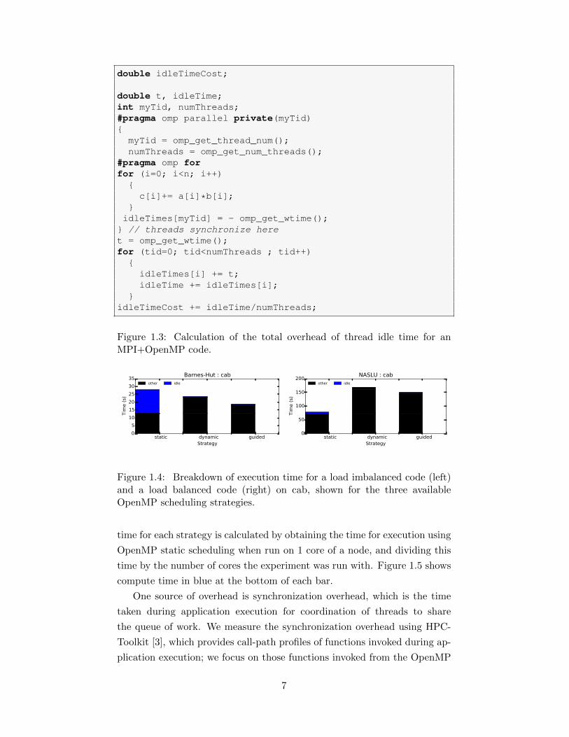
Figure 1.4 shows the performance of different OpenMP scheduling strate-
gies for Barnes-Hut and NAS LU. The OpenMP dynamic strategies make
the performance substantially worse for NAS LU, and do not improve it to
the extent expected for Barnes-Hut, as explained below. The first challenge
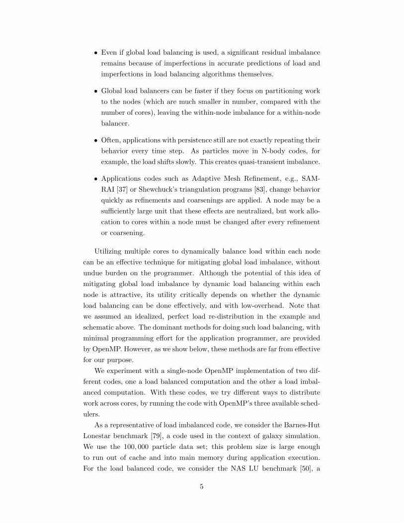
for any load balancing strategy is in handling thread idle times due to load
imbalances from the application or architecture. The method used to obtain
the idle time is shown in Figure 1.3. The average thread idle time shown
in blue in Figure 1.4 is the sum of idle times across all cores divided by the
number of cores. The other time, shown in black, is average computation
time per core, calculated as the difference between (a) the sum of execu-
tion times divided by the number of cores, and (b) the average thread idle
time. Note that the sum of idle times across threads is the load imbalance
that could be avoided. Thus, the average idle time across all threads is the
overhead of idle time incurred during application execution. One might ex-
pect that dynamic scheduling would eliminate thread idle time. However,
idle time can exist in dynamic scheduling due to task quantization [54], i.e.,
even with dynamic scheduling, each core except one may have idle time as
large as the size of each dynamically scheduled task (a task is a chunk of
iterations assigned at once).
The dynamic scheduling almost completely eliminated idle time for
Barnes-Hut, but the total execution did not go down by the same amount,
i.e., the black portion of the bar increased. For NAS LU, the execution time
in both dynamic strategies is substantially worse than the static strategy.
What are the remaining overheads that cause the increased execution
time in Figure 1.4? We first isolate the compute time of the application
execution time, or the time spent doing the application’s work. The compute
6
double idleTimeCost;
double t, idleTime;int myTid, numThreads;#pragma omp parallel private(myTid){
myTid = omp_get_thread_num();numThreads = omp_get_num_threads();
#pragma omp forfor (i=0; i<n; i++)
{c[i]+= a[i]*b[i];
}idleTimes[myTid] = - omp_get_wtime();
} // threads synchronize heret = omp_get_wtime();for (tid=0; tid<numThreads ; tid++)
{idleTimes[i] += t;idleTime += idleTimes[i];
}idleTimeCost += idleTime/numThreads;
Figure 1.3: Calculation of the total overhead of thread idle time for anMPI+OpenMP code.
static dynamic guidedStrategy
0
5
10
15
20
25
30
35
Tim
e (
s)
Barnes-Hut : cabother idle
static dynamic guidedStrategy
0
50
100
150
200
Tim
e (
s)
NASLU : cabother idle
Figure 1.4: Breakdown of execution time for a load imbalanced code (left)and a load balanced code (right) on cab, shown for the three availableOpenMP scheduling strategies.
time for each strategy is calculated by obtaining the time for execution using
OpenMP static scheduling when run on 1 core of a node, and dividing this
time by the number of cores the experiment was run with. Figure 1.5 shows
compute time in blue at the bottom of each bar.
One source of overhead is synchronization overhead, which is the time
taken during application execution for coordination of threads to share
the queue of work. We measure the synchronization overhead using HPC-
Toolkit [3], which provides call-path profiles of functions invoked during ap-
plication execution; we focus on those functions invoked from the OpenMP
7
static dynamic guidedStrategy
0
5
10
15
20
25
30
35
Tim
e (
s)
Barnes-Hut : cabcomp other dq idle
static dynamic guidedStrategy
0
50
100
150
200
Tim
e (
s)
NASLU : cabcomp other dq idle
Figure 1.5: Breakdown of time. Synchronization overheads are shown ingreen.
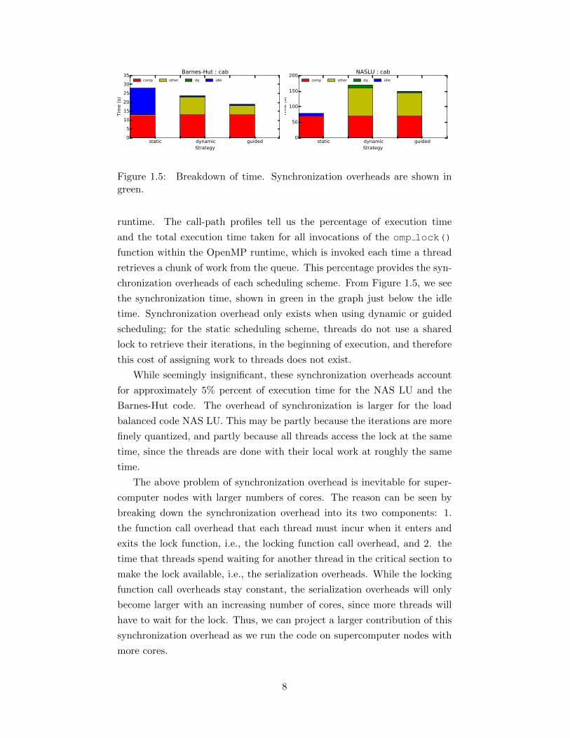
runtime. The call-path profiles tell us the percentage of execution time
and the total execution time taken for all invocations of the omp lock()
function within the OpenMP runtime, which is invoked each time a thread
retrieves a chunk of work from the queue. This percentage provides the syn-
chronization overheads of each scheduling scheme. From Figure 1.5, we see
the synchronization time, shown in green in the graph just below the idle
time. Synchronization overhead only exists when using dynamic or guided
scheduling; for the static scheduling scheme, threads do not use a shared
lock to retrieve their iterations, in the beginning of execution, and therefore
this cost of assigning work to threads does not exist.
While seemingly insignificant, these synchronization overheads account
for approximately 5% percent of execution time for the NAS LU and the
Barnes-Hut code. The overhead of synchronization is larger for the load
balanced code NAS LU. This may be partly because the iterations are more
finely quantized, and partly because all threads access the lock at the same
time, since the threads are done with their local work at roughly the same
time.
The above problem of synchronization overhead is inevitable for super-
computer nodes with larger numbers of cores. The reason can be seen by
breaking down the synchronization overhead into its two components: 1.
the function call overhead that each thread must incur when it enters and
exits the lock function, i.e., the locking function call overhead, and 2. the
time that threads spend waiting for another thread in the critical section to
make the lock available, i.e., the serialization overheads. While the locking
function call overheads stay constant, the serialization overheads will only
become larger with an increasing number of cores, since more threads will
have to wait for the lock. Thus, we can project a larger contribution of this
synchronization overhead as we run the code on supercomputer nodes with
more cores.
8
However, as can be seen in Figure 1.5, the synchronization overhead
alone does not account completely for the performance degradation with
OpenMP dynamic scheduling and OpenMP guided scheduling. Since dy-
namic scheduling may lead to accessing a cache line that may be in another
core’s cache, the remaining overheads are likely from data movement.
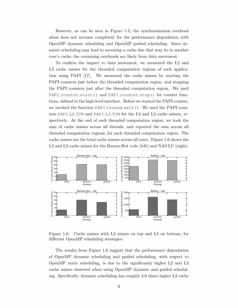
To confirm the impact to data movement, we measured the L2 and
L3 cache misses for the threaded computation regions of each applica-
tion using PAPI [17]. We measured the cache misses by starting the
PAPI counters just before the threaded computation region, and stopping
the PAPI counters just after the threaded computation region. We used
PAPI counter start() and PAPI counter stop() for counter func-
tions, defined in the high-level interface. Before we started the PAPI counter,
we invoked the function PAPI thread self(). We used the PAPI coun-
ters PAPI L2 TCM and PAPI L3 TCM for the L2 and L3 cache misses, re-
spectively. At the end of each threaded computation region, we took the
sum of cache misses across all threads, and reported the sum across all
threaded computation regions, for each threaded computation region. The
cache misses are the total cache misses across all cores. Figure 1.6 shows the
L2 and L3 cache misses for the Barnes-Hut code (left) and NAS LU (right).
static dynamic guidedStrategy
0
10
20
30
40
50
60
L2 C
ach
e M
isse
s (m
illio
ns)
Barnes-Hut : cab
static dynamic guidedStrategy
500
1000
1500
2000
2500
3000
3500
4000
L2 C
ach
e M
isse
s (m
illio
ns)
NASLU : cab
static dynamic guidedStrategy
0
5
10
15
20
25
30
L3 C
ach
e M
isse
s (m
illio
ns)
Barnes-Hut : cab
static dynamic guidedStrategy
500
1000
1500
2000
L3 C
ach
e M
isse
s (m
illio
ns)
NASLU : cab
Figure 1.6: Cache misses with L2 misses on top and L3 on bottom, fordifferent OpenMP scheduling strategies.
The results from Figure 1.6 suggest that the performance degradation
of OpenMP dynamic scheduling and guided scheduling, with respect to
OpenMP static scheduling, is due to the significantly higher L2 and L3
cache misses observed when using OpenMP dynamic and guided schedul-
ing. Specifically, dynamic scheduling has roughly 4.0 times higher L2 cache
9
misses over static scheduling, and 3.5 times higher L3 cache misses over
static scheduling. The cost of data movement does not decrease signifi-
cantly with OpenMP guided scheduling. OpenMP guided scheduling has
3.5 times higher L2 cache misses compared to OpenMP static scheduling,
and 2.8 times higher L3 cache misses compared to OpenMP static schedul-
ing. The cost of coherence cache misses increases with increasing numbers
of cores. The reason is that the probability that a core selects a tasklet that
it did not execute in the last invocation of the threaded computation region
(this incurs coherence cache misses) increases with increasing numbers of
cores.
1.1 Cache Miss Calculations
To check that the cache misses in Figure 1.6 are in fact impacting perfor-
mance and can explain most of the performance loss quantitatively, we show
calculations for NAS LU. We obtain the time for an L2 cache miss and for an
L3 cache miss on Cab using the specification sheet for Cab’s node architec-
ture [60], along with Intel’s forum post reply referring to this specification
sheet that gives the information needed [24]. In the architecture specifica-
tion sheet, the processor frequency is 2.66GHz. The forum post indicates
that the L2 remote cache miss latency is 100-300 cycles, so we use the mean
cycle time of 200 cycles. The time to remote DRAM, i.e., the L3 cache miss
latency, is 100 nanoseconds.
We need to account for 485.52 - 83.53 - 24.65 = 376 seconds of time
spent in dynamic scheduling. Note that we do not need the execution time
breakdown here, since this code exhibits low idle time. Cache miss time for
the L2 cache is 2002.66×109 · (3845×106−2257×106) = 65 seconds. This leaves
376 - 65 = 311 seconds to account for. Cache miss time for the L3 cache is
(100 ·10−9) ·(1676−631)×106 = 97 seconds. This now leaves 311 - 97 = 214
seconds to account for. The time of L3 cache misses may be much higher
than 100 nanoseconds, because access to main memory by multiple threads
requires threads to wait in the memory queue. In the worst case, i.e., when
all threads access main memory simultaneously, the latency to memory is a
factor of (16 + (16−mem queue depth)× 100) nanoseconds of the original
latency, where mem queue depth = 12 on this machine.
To check that memory bandwidth was the factor for the increase in time
for L3 cache misses, we ran STREAM [66] on one core of Cab and on all cores
10
of Cab. We recorded the bandwidth for both runs. The memory bandwidth
of STREAM triad run on one core is 14,837.24 MB/s, but the memory
bandwidth of STREAM triad run on 16 cores is only 103,669.71 MB/s, a 7x
improvement in memory bandwidth rather than a 16x improvement. The
effective memory latency increases by a factor of 2.4x, giving 238 seconds
instead of 97 seconds for the cache miss time for L3. The remaining time is
now 311 - 238 = 73 seconds. This may be due to the L2 cache miss latency
being higher (also, note that the L2 cache miss latency was reported at 1
core). Another cause could be TLB misses, although we to tried reduce their
impact by using huge pages for the runs.
While the above is a rough estimate, it helps explain the performance
degradation. Additionally, in terms of order of magnitude, the calculations
show that the timings shown in yellow for NAS LU in Figure 1.5 are mostly
attributed to data movement.
Thus, current OpenMP schedulers do not solve the performance problem
for next-generation clusters of SMPs. We have identified three challenges to
obtaining good performance using dynamic load balancing within a node:
(1) idle time due to load imbalances from the application or system noise, (2)
data movement overhead, and (3) synchronization overheads from runtimes.
These challenges provide motivations for developing a new set of schedulers,
which balance the tradeoff between load balance and locality that works for
any application-architecture pair.
To summarize, we first argued for the importance of handling within-
node load imbalances, and how they could mitigate the performance
loss due to global load imbalances. We describe these schematically for
both transient and persistent imbalances, using NAS LU and N-body
code, respectively. We further showed that using OpenMP scheduling
strategies to do this dynamic load balancing is problematic because they
add significant data movement overheads. Given the above challenges, the
objective of this thesis is to:
Design a set of new scheduling strategies that handles all three causes
of performance loss, i.e., thread idle time, data movement, and synchro-
nization overhead, simultaneously, for any application and architecture, in
the context of an MPI+OpenMP application.
11
Thus, we ask: can we combine a static and dynamic scheduling scheme
that simultaneously reduces load imbalances and scheduler overhead, in an
intelligent manner?
The key idea of our solution is to allocate to threads a fixed fraction of
OpenMP loop iterations statically, and schedule the remainder dynamically.
We define the ratio of static loop iterations to all loop iterations as the static
fraction (and the ratio of dynamic iterations to all iterations as the dynamic
fraction). The scheduling schemes developed throughout this thesis are an
elaboration of this basic idea.
1.2 Contributions
The main contributions of this thesis are:
• An experimental method to determine parameter values of our strategy
which achieves the tradeoff between load balance and locality;
• A runtime determination of scheduler parameters for maximizing both
load balance and locality, given partially transient and partially per-
sistent load imbalance;
• A performance model and theoretical analysis of scheduler parameter
values for our strategy for any number of nodes;
• analysis and experimentation of the tradeoff between locality and load
balance for coarse-grained application-generated imbalances;
• A methodology to provide for continual innovation of new scheduling
strategies through a combination of basic strategies developed, and to
provide a way to integrate into existing OpenMP or MPI runtimes, or
any exascale runtime.
Low-overhead dynamic scheduling has far-reaching implications because it
allows us to utilize the existence of multiple cores on a node to mitigate the
effects of load imbalances. Since the number of cores is expected to grow far
more rapidly than the number of nodes in future generations of hardware [9,
29, 78], future machines will be able to prevent effects of load imbalances
from propagating to other nodes by off-loading delayed work to other cores
within the node. If integrated with MPI and OpenMP implementations,
our techniques will avoid the scaling wall due to load imbalances for several
generations of machines to come.
12
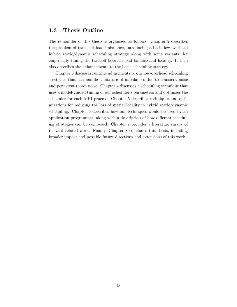
1.3 Thesis Outline
The remainder of this thesis is organized as follows. Chapter 2 describes
the problem of transient load imbalance, introducing a basic low-overhead
hybrid static/dynamic scheduling strategy along with some variants, for
empirically tuning the tradeoff between load balance and locality. It then
also describes the enhancements to the basic scheduling strategy.
Chapter 3 discusses runtime adjustments to our low-overhead scheduling
strategies that can handle a mixture of imbalances due to transient noise
and persistent (core) noise. Chapter 4 discusses a scheduling technique that
uses a model-guided tuning of our scheduler’s parameters and optimizes the
scheduler for each MPI process. Chapter 5 describes techniques and opti-
mizations for reducing the loss of spatial locality in hybrid static/dynamic
scheduling. Chapter 6 describes how our techniques would be used by an
application programmer, along with a description of how different schedul-
ing strategies can be composed. Chapter 7 provides a literature survey of
relevant related work. Finally, Chapter 8 concludes this thesis, including
broader impact and possible future directions and extensions of this work.
13
Chapter 2
Hybrid Static/DynamicScheduling
In the previous chapter, we highlighted three challenges for current OpenMP
loop schedulers. In this chapter, we show an intuitive diagram and model
for OpenMP static scheduling and OpenMP dynamic scheduling. With this,
we present our solution of mixed static/dynamic scheduling using OpenMP
static and dynamic scheduling to obtain the benefits of static and dynamic
scheduling, which can address the challenges of static and dynamic schedul-
ing. Given this mixed static/dynamic scheduling scheme, we ask how to
select the static fraction, and suggest a basic strategy of exhaustive search.
We apply the resulting scheduling strategy to the NAS LU and Barnes-Hut
code in Chapter 1. We proceed to describe a 3D regular mesh code, and
apply our static/dynamic scheduling technique to this code. In this part
of the chapter, we describe our own implemented scheduling library, which
allows for providing locality across timesteps for the dynamic section of the
scheduler, and allows for simultaneously tuning different parameters of the
scheduler. Finally, we discuss our approach applied to dense matrix fac-
torizations, highlighting a Communication-Avoiding LU code which has our
hybrid static/dynamic scheduling approach applied to it. We particularly
show its competitive performance over two widely-known implementations of
LU factorization, one from Intel’s MKL library for numerical linear algebra
codes, and the other from University of Tennessee’s PLASMA runtime.
2.1 Basic Mixed Static/Dynamic Scheduling
Technique
Given the thesis objective to design a set of new scheduling strategies that
handle all three causes of the problem, i.e., thread idle time, data movement,
and synchronization overhead, simultaneously, for many applications and
platforms, in the context of an MPI+OpenMP application, we propose a
new scheduling scheme.
Figure 2.1 shows a schematic of an OpenMP statically scheduled
14
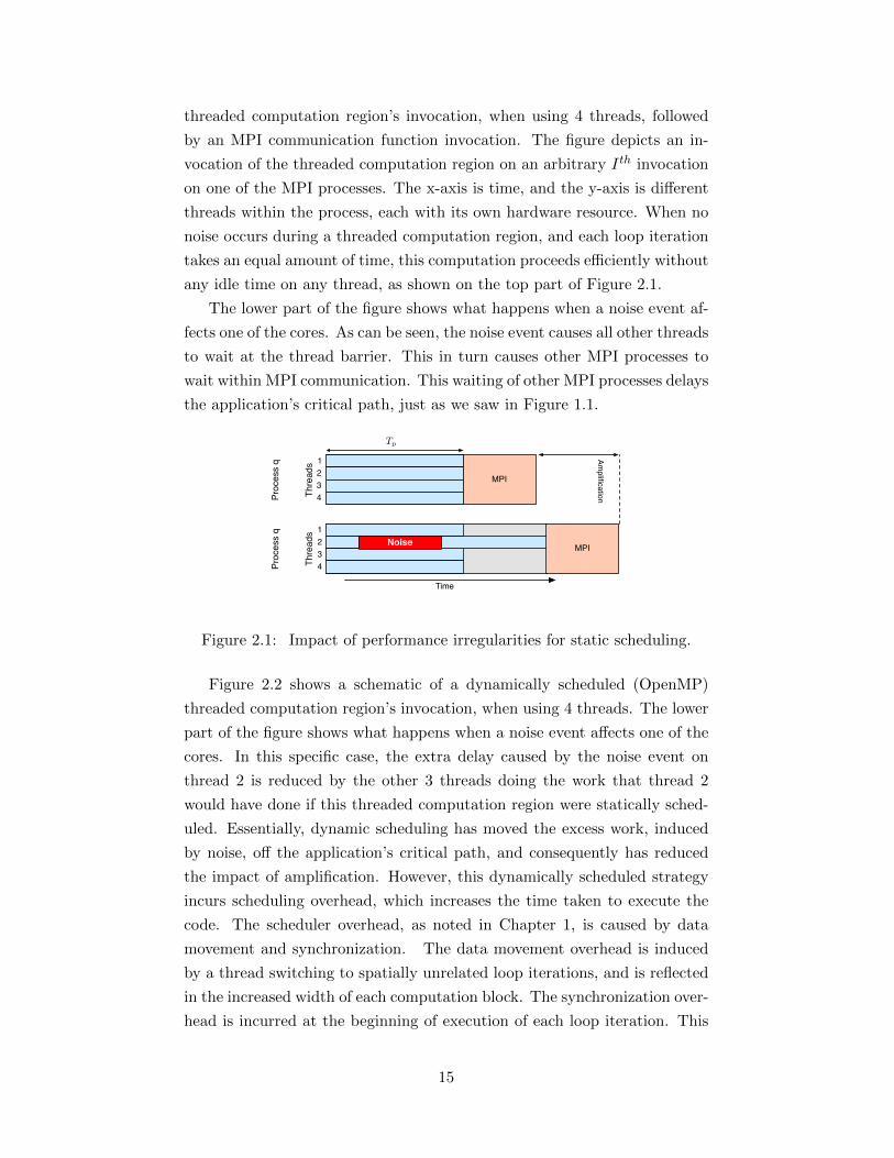
threaded computation region’s invocation, when using 4 threads, followed
by an MPI communication function invocation. The figure depicts an in-
vocation of the threaded computation region on an arbitrary Ith invocation
on one of the MPI processes. The x-axis is time, and the y-axis is different
threads within the process, each with its own hardware resource. When no
noise occurs during a threaded computation region, and each loop iteration
takes an equal amount of time, this computation proceeds efficiently without
any idle time on any thread, as shown on the top part of Figure 2.1.
The lower part of the figure shows what happens when a noise event af-
fects one of the cores. As can be seen, the noise event causes all other threads
to wait at the thread barrier. This in turn causes other MPI processes to
wait within MPI communication. This waiting of other MPI processes delays
the application’s critical path, just as we saw in Figure 1.1.
MPI
1234
1234
Time
Amplification
Noise MPI
Tp
Thre
ads
Thre
ads
Proc
ess
qPr
oces
s q
Figure 2.1: Impact of performance irregularities for static scheduling.
Figure 2.2 shows a schematic of a dynamically scheduled (OpenMP)
threaded computation region’s invocation, when using 4 threads. The lower
part of the figure shows what happens when a noise event affects one of the
cores. In this specific case, the extra delay caused by the noise event on
thread 2 is reduced by the other 3 threads doing the work that thread 2
would have done if this threaded computation region were statically sched-
uled. Essentially, dynamic scheduling has moved the excess work, induced
by noise, off the application’s critical path, and consequently has reduced
the impact of amplification. However, this dynamically scheduled strategy
incurs scheduling overhead, which increases the time taken to execute the
code. The scheduler overhead, as noted in Chapter 1, is caused by data
movement and synchronization. The data movement overhead is induced
by a thread switching to spatially unrelated loop iterations, and is reflected
in the increased width of each computation block. The synchronization over-
head is incurred at the beginning of execution of each loop iteration. This
15
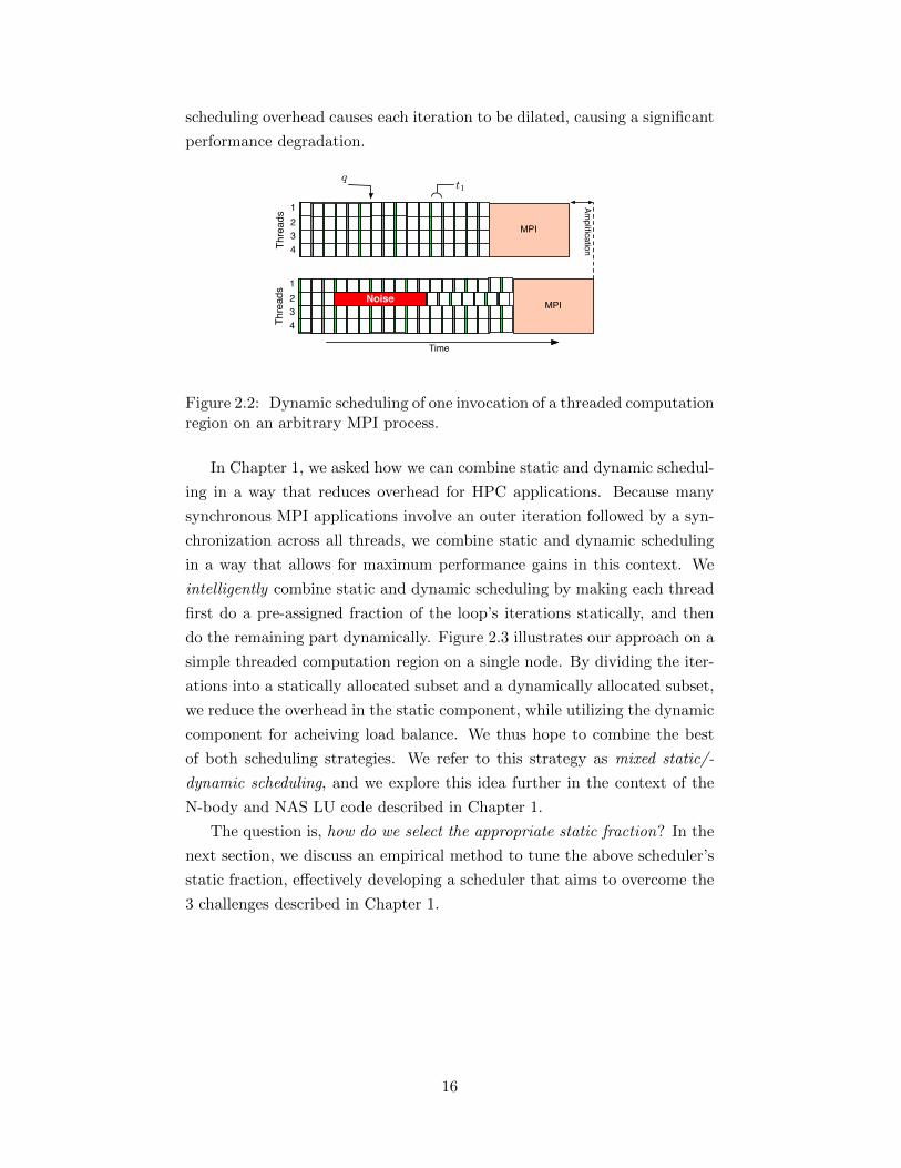
scheduling overhead causes each iteration to be dilated, causing a significant
performance degradation.
1234
Time
1234
Noise
MPI
MPIAm
plification
t1q
Threads
Threads
Figure 2.2: Dynamic scheduling of one invocation of a threaded computationregion on an arbitrary MPI process.
In Chapter 1, we asked how we can combine static and dynamic schedul-
ing in a way that reduces overhead for HPC applications. Because many
synchronous MPI applications involve an outer iteration followed by a syn-
chronization across all threads, we combine static and dynamic scheduling
in a way that allows for maximum performance gains in this context. We
intelligently combine static and dynamic scheduling by making each thread
first do a pre-assigned fraction of the loop’s iterations statically, and then
do the remaining part dynamically. Figure 2.3 illustrates our approach on a
simple threaded computation region on a single node. By dividing the iter-
ations into a statically allocated subset and a dynamically allocated subset,
we reduce the overhead in the static component, while utilizing the dynamic
component for acheiving load balance. We thus hope to combine the best
of both scheduling strategies. We refer to this strategy as mixed static/-
dynamic scheduling, and we explore this idea further in the context of the
N-body and NAS LU code described in Chapter 1.
The question is, how do we select the appropriate static fraction? In the
next section, we discuss an empirical method to tune the above scheduler’s
static fraction, effectively developing a scheduler that aims to overcome the
3 challenges described in Chapter 1.
16
1234
1234
Time
Noise
MPI
MPI
Amplification
t1qfs · Tp
Threads
Threads
Figure 2.3: Using mixed static/dynamic scheduling to handle load imbal-ances across cores.
2.2 Results for Barnes-Hut and NAS LU with
Mixed Static/Dynamic Scheduling
As a first approximation for the static fraction for the scheduler, we choose
50%. This can be implemented by splitting the data parallel loop shown in
Figure 2.4 into two OpenMP loops: the first statically scheduled, and the
second dynamically scheduled, as shown in Figure 2.5.
#pragma omp parallel for schedule(static)for(int i=0; i<n; i++)
c[i] += a[i]*b[i];
Figure 2.4: OpenMP loop with static scheduling.
#pragma omp parallel for nowaitfor (int i = 0; i < n/2; i++)
c[i] += a[i]*b[i];
#pragma omp parallel for schedule(dynamic)for (int i = n/2; i < n; i++)
c[i] += a[i]*b[i];
Figure 2.5: OpenMP loop modified for mixed static/dynamic scheduling.
We refer to this strategy as Mixed Static/Dynamic Scheduling, and label
it half in the graphs for brevity. We expect half to cut the dynamic schedul-
ing overhead in half. Figure 2.6 shows the performance of this strategy along
with multiple OpenMP strategies on Cab for Barnes-Hut and NASLU codes.
For the Barnes-Hut code, the half scheduling improves performance 10.1%
17
static dynamic guided halfStrategy
0
5
10
15
20
25
30
35
Tim
e (
s)
Barnes-Hut : cabcomp dm dq idle
static dynamic guided halfStrategy
0
50
100
150
200
Tim
e (
s)
NASLU : cabcomp dm dq idle
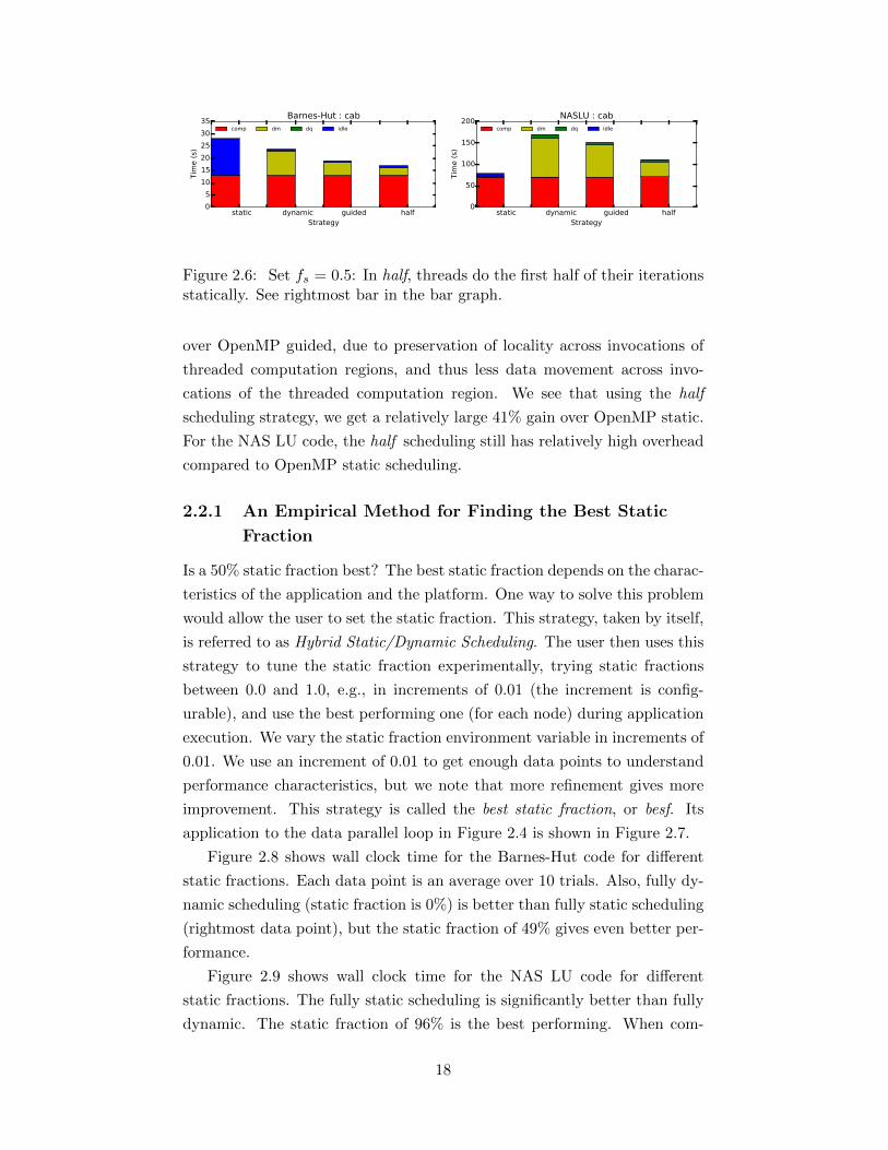
Figure 2.6: Set fs = 0.5: In half, threads do the first half of their iterationsstatically. See rightmost bar in the bar graph.
over OpenMP guided, due to preservation of locality across invocations of
threaded computation regions, and thus less data movement across invo-
cations of the threaded computation region. We see that using the half
scheduling strategy, we get a relatively large 41% gain over OpenMP static.
For the NAS LU code, the half scheduling still has relatively high overhead
compared to OpenMP static scheduling.
2.2.1 An Empirical Method for Finding the Best Static
Fraction
Is a 50% static fraction best? The best static fraction depends on the charac-
teristics of the application and the platform. One way to solve this problem
would allow the user to set the static fraction. This strategy, taken by itself,
is referred to as Hybrid Static/Dynamic Scheduling. The user then uses this
strategy to tune the static fraction experimentally, trying static fractions
between 0.0 and 1.0, e.g., in increments of 0.01 (the increment is config-
urable), and use the best performing one (for each node) during application
execution. We vary the static fraction environment variable in increments of
0.01. We use an increment of 0.01 to get enough data points to understand
performance characteristics, but we note that more refinement gives more
improvement. This strategy is called the best static fraction, or besf. Its
application to the data parallel loop in Figure 2.4 is shown in Figure 2.7.
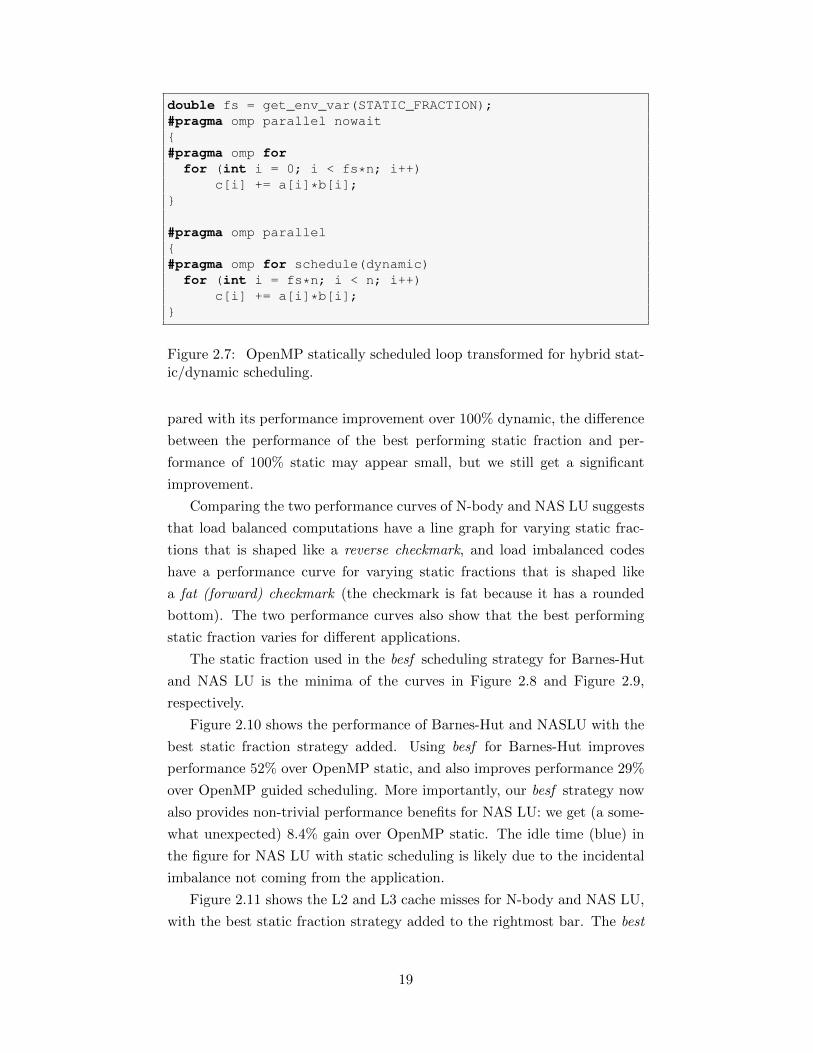
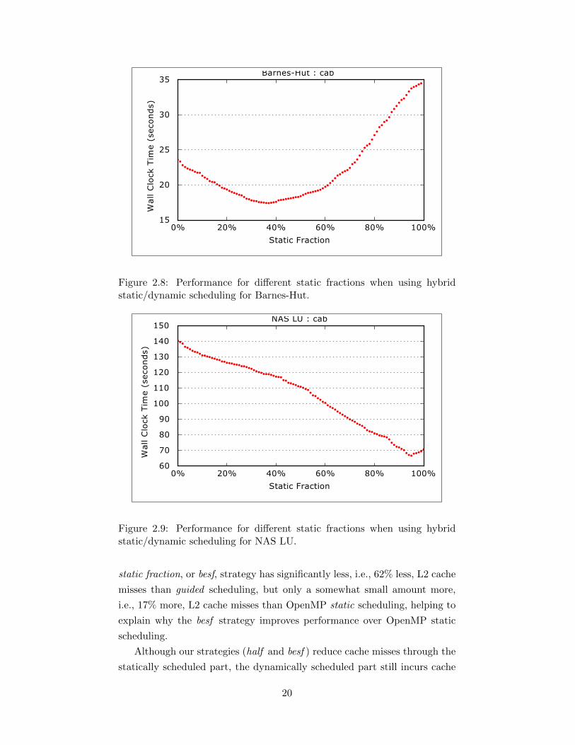
Figure 2.8 shows wall clock time for the Barnes-Hut code for different
static fractions. Each data point is an average over 10 trials. Also, fully dy-
namic scheduling (static fraction is 0%) is better than fully static scheduling
(rightmost data point), but the static fraction of 49% gives even better per-
formance.
Figure 2.9 shows wall clock time for the NAS LU code for different
static fractions. The fully static scheduling is significantly better than fully
dynamic. The static fraction of 96% is the best performing. When com-
18
double fs = get_env_var(STATIC_FRACTION);#pragma omp parallel nowait{#pragma omp for
for (int i = 0; i < fs*n; i++)c[i] += a[i]*b[i];
}
#pragma omp parallel{#pragma omp for schedule(dynamic)
for (int i = fs*n; i < n; i++)c[i] += a[i]*b[i];
}
Figure 2.7: OpenMP statically scheduled loop transformed for hybrid stat-ic/dynamic scheduling.
pared with its performance improvement over 100% dynamic, the difference
between the performance of the best performing static fraction and per-
formance of 100% static may appear small, but we still get a significant
improvement.
Comparing the two performance curves of N-body and NAS LU suggests
that load balanced computations have a line graph for varying static frac-
tions that is shaped like a reverse checkmark, and load imbalanced codes
have a performance curve for varying static fractions that is shaped like
a fat (forward) checkmark (the checkmark is fat because it has a rounded
bottom). The two performance curves also show that the best performing
static fraction varies for different applications.
The static fraction used in the besf scheduling strategy for Barnes-Hut
and NAS LU is the minima of the curves in Figure 2.8 and Figure 2.9,
respectively.
Figure 2.10 shows the performance of Barnes-Hut and NASLU with the
best static fraction strategy added. Using besf for Barnes-Hut improves
performance 52% over OpenMP static, and also improves performance 29%
over OpenMP guided scheduling. More importantly, our besf strategy now
also provides non-trivial performance benefits for NAS LU: we get (a some-
what unexpected) 8.4% gain over OpenMP static. The idle time (blue) in
the figure for NAS LU with static scheduling is likely due to the incidental
imbalance not coming from the application.
Figure 2.11 shows the L2 and L3 cache misses for N-body and NAS LU,
with the best static fraction strategy added to the rightmost bar. The best
19
0% 20% 40% 60% 80% 100%
Static Fraction
15
20
25
30
35
Wall
Clo
ck T
ime (
seco
nds)
Barnes-Hut : cab
Figure 2.8: Performance for different static fractions when using hybridstatic/dynamic scheduling for Barnes-Hut.
0% 20% 40% 60% 80% 100%
Static Fraction
60
70
80
90
100
110
120
130
140
150
Wall
Clo
ck T
ime (
seco
nds)
NAS LU : cab
Figure 2.9: Performance for different static fractions when using hybridstatic/dynamic scheduling for NAS LU.
static fraction, or besf, strategy has significantly less, i.e., 62% less, L2 cache
misses than guided scheduling, but only a somewhat small amount more,
i.e., 17% more, L2 cache misses than OpenMP static scheduling, helping to
explain why the besf strategy improves performance over OpenMP static
scheduling.
Although our strategies (half and besf ) reduce cache misses through the
statically scheduled part, the dynamically scheduled part still incurs cache
20

static dynamic guided half besfStrategy
0
5
10
15
20
25
30
35
Tim
e (
s)
Barnes-Hut : cabcomp dm dq idle
static dynamic guided half besfStrategy
0
50
100
150
200
Tim
e (
s)
NASLU : cabcomp dm dq idle
Figure 2.10: Execution time breakdown with the besf strategy added onthe rightmost bar.
static dynamic guided half besfStrategy
0
10
20
30
40
50
60
L2 C
ach
e M
isse
s (m
illio
ns)
static dynamic guided half besfStrategy
500
1000
1500
2000
2500
3000
3500
4000
L2 C
ach
e M
isse
s (m
illio
ns)
static dynamic guided half besfStrategy
0
5
10
15
20
25
30
L3 C
ach
e M
isse
s (m
illio
ns)
Barnes-Hut : cab
static dynamic guided half besfStrategy
500
1000
1500
2000
L3 C
ach
e M
isse
s (m
illio
ns)
NASLU : cab
Figure 2.11: L2 cache misses shown in the top graphs; L3 in the bottom.The best static fraction strategy is added on the rightmost bar.
misses because of the loss of spatial locality. We describe a scheme to reduce
these further in Chapter 5.
We next apply our strategy, with empirical determination of best static
fraction, to several NAS benchmarks. Table 2.1 and Table 2.2 respec-
tively show the performance improvement of our scheduling technique over
OpenMP static scheduling on the NAS benchmarks for an Intel Westmere
16-core node (cab) and an IBM BG/Q 16-core node (rzuseq). As can be seen
in Table 2.1, the gains for the CG benchmark are large on the Intel West-
mere machine due to the scheduler’s handling of application load imbalance
of NAS CG along with load imbalance due to performance irregularities
arising from OS noise. As seen in Table 2.2, while the BG/Q machine has
low noise [12], the scheduler still achieves significant performance gains for
CG because of its ability to handle the application load imbalance of CG.
21
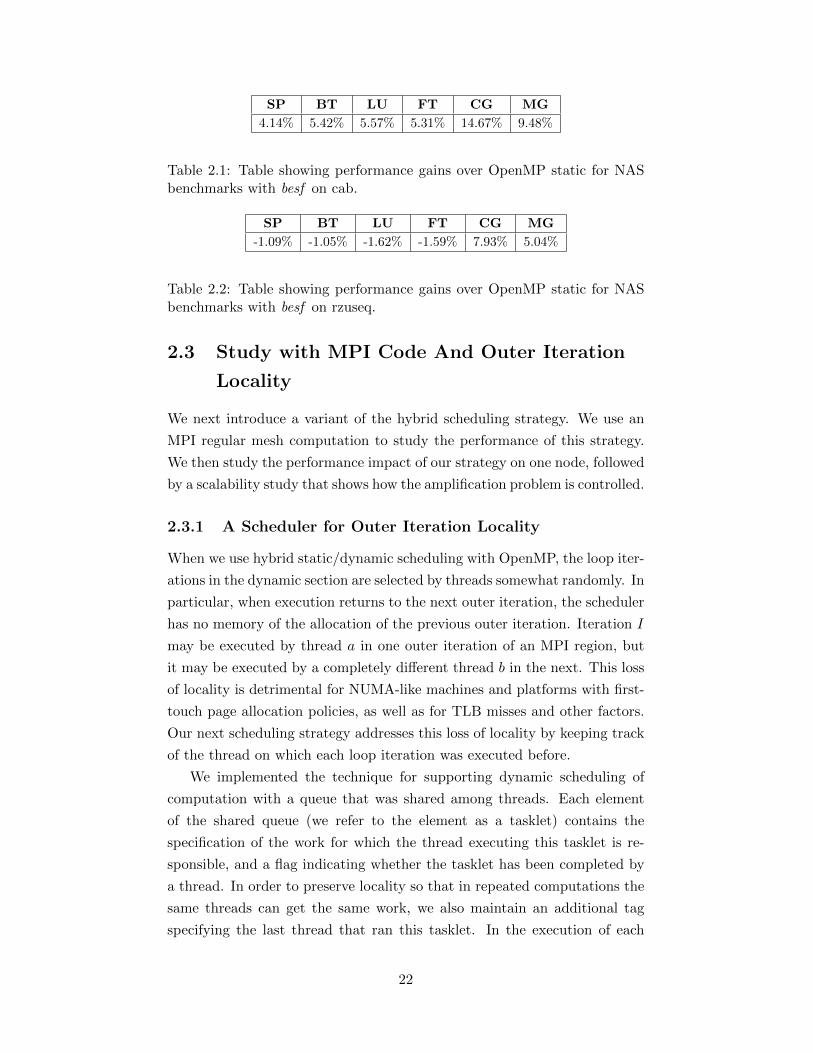
SP BT LU FT CG MG
4.14% 5.42% 5.57% 5.31% 14.67% 9.48%
Table 2.1: Table showing performance gains over OpenMP static for NASbenchmarks with besf on cab.
SP BT LU FT CG MG
-1.09% -1.05% -1.62% -1.59% 7.93% 5.04%
Table 2.2: Table showing performance gains over OpenMP static for NASbenchmarks with besf on rzuseq.
2.3 Study with MPI Code And Outer Iteration
Locality
We next introduce a variant of the hybrid scheduling strategy. We use an
MPI regular mesh computation to study the performance of this strategy.
We then study the performance impact of our strategy on one node, followed
by a scalability study that shows how the amplification problem is controlled.
2.3.1 A Scheduler for Outer Iteration Locality
When we use hybrid static/dynamic scheduling with OpenMP, the loop iter-
ations in the dynamic section are selected by threads somewhat randomly. In
particular, when execution returns to the next outer iteration, the scheduler
has no memory of the allocation of the previous outer iteration. Iteration I
may be executed by thread a in one outer iteration of an MPI region, but
it may be executed by a completely different thread b in the next. This loss
of locality is detrimental for NUMA-like machines and platforms with first-
touch page allocation policies, as well as for TLB misses and other factors.
Our next scheduling strategy addresses this loss of locality by keeping track
of the thread on which each loop iteration was executed before.
We implemented the technique for supporting dynamic scheduling of
computation with a queue that was shared among threads. Each element
of the shared queue (we refer to the element as a tasklet) contains the
specification of the work for which the thread executing this tasklet is re-
sponsible, and a flag indicating whether the tasklet has been completed by
a thread. In order to preserve locality so that in repeated computations the
same threads can get the same work, we also maintain an additional tag
specifying the last thread that ran this tasklet. In the execution of each
22
iteration of an MPI+pthreads program, there are 3 repeated phases: MPI
communication, statically scheduled computation, and dynamically sched-
uled computation. In the first phase, thread 0 does the MPI communication
for border exchange. During this time, all other threads typically wait at
a thread barrier. In the second phase, each thread does all work that is
statically allocated to it. Once a thread completes its statically allocated
work, it immediately moves to the third phase, where it starts retrieving the
next available tasklet from the queue shared among other threads, which it
repeats until the queue is empty. As in the completely static scheduled case,
after threads have finished computation, they must wait at a barrier before
continuing to the next iteration. The percentage of dynamic work, granu-
larity/number of tasklets, and number of queues per node, are specified as
parameters.
An additional scheme extends this strategy to improve outer iteration
locality. In this scheme, each tasklet in the queue has an extra field, or tag,
that records the thread ID that executed the tasklet in the previous outer
iteration. In the third phase, when a thread retrieves a tasklet from the
queue, the scheduler attempts to first give it a tasklet having a tag equal
to its thread ID. Only if such a tasklet is not available are other tasklets
assigned. We refer to this strategy as scheduling with locality tags, or simply
scheduling with locality.
2.3.2 MPI Regular Mesh Computation
Our model application is an exemplar of regular mesh code. For simplicity,
we will call it a Jacobi algorithm, as the work that we perform in our model
problem is the Jacobi relaxation iteration in solving a Poisson problem.
However, the data and computational pattern are similar for both regular
mesh codes (both implicit and explicit) and for algorithms that attempt
to divide work evenly among processor cores (such as most sparse matrix-
vector multiply implementations). Many MPI implmentations of regular
mesh codes traditionally have a pre-defined domain decomposition, as is seen
in many libraries and microbenchmark suites [86]. This optimal decomposi-
tion is necessary to reduce communication overhead, minimize cache misses,
and ensure data locality. In this work, we consider a slab decomposition of
a 3-dimensional block implemented in an MPI/pthreads hybrid model, an
increasingly popular model for taking advantage of clusters of SMPs. We
use a problem size and dimension that can highlight many of the issues that
we see in real-world applications with mesh computations implemented in
23
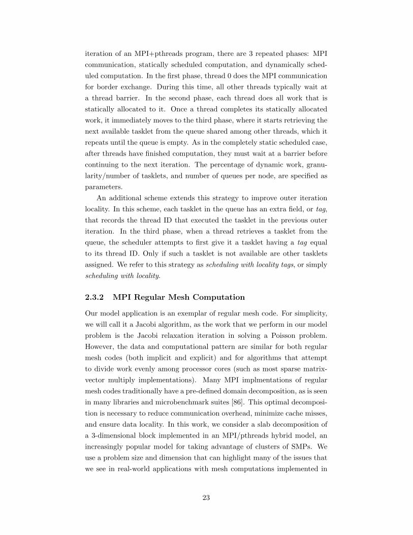
MPI: specifically, we use a 3D block with dimensions 64× 512× 64 on each
node for a fixed 1000 iterations. With this problem size, we can ensure that
computations are done out-of-cache so that it is just enough to excercise the
full memory hierarchy. The block is partitioned into vertical slabs across
processes along the X dimension. Each vertical slab is further partitioned
into horizontal slabs across threads along the Y dimension. The slab domain
decomposition across processes is shown in Figure 2.12, while the full hybrid
process-thread domain decomposition is shown in Figure 2.13.
MPI_Isend
3D Poisson Problem(slab)
P0 P1 Pn
yDim
zDim
xDim
MPI_IrecvMPI_Irecv
MPI_Isend
Figure 2.12: 3D stencil domain decomposition across MPI processes.
We use the slab decomposition strategy for the regular mesh because
of its simplicity to implement and to tune parameters in our search space,
and because it is a common way to partition meshes in Lattice-Boltzmann
codes [93]. A MPI border exchange communication occurs between left and
right borders of blocks of each process across the YZ planes. The border
exchange operation uses an MPI Isend and MPI Irecv pair, along with an
MPI Waitall. We mitigate the issue of first-touch as noted in [78] by doing
parallel memory allocation during the initialization of our mesh. For such
regular mesh computations, the communication between processes, even in
an explicit mesh sweep, provides a synchronization between the processes.
Any load imbalance between the processes can be amplified, even when using
a good (but static) domain decomposition strategy. If even 1% of nodes are
24

Static Decomposition (r =0.0)
P0 P1
Task0 Æ thread 0
Task 1 Æthread 1
StaticTaskSize
Task tÆ thread t
Figure 2.13: 3D stencil domain decomposition across MPI processes, alongwith thread partitioning of work within each MPI process.
affected by system interference during one iteration of a computationally
intensive MPI application on a cluster with 1000s of nodes, several nodes
will be affected by noise during each iteration. Our solution to this problem
is presented in the section that follows.
Figure 2.14: Histograms for static scheduling on 1 node, showing bi-modaldistribution.
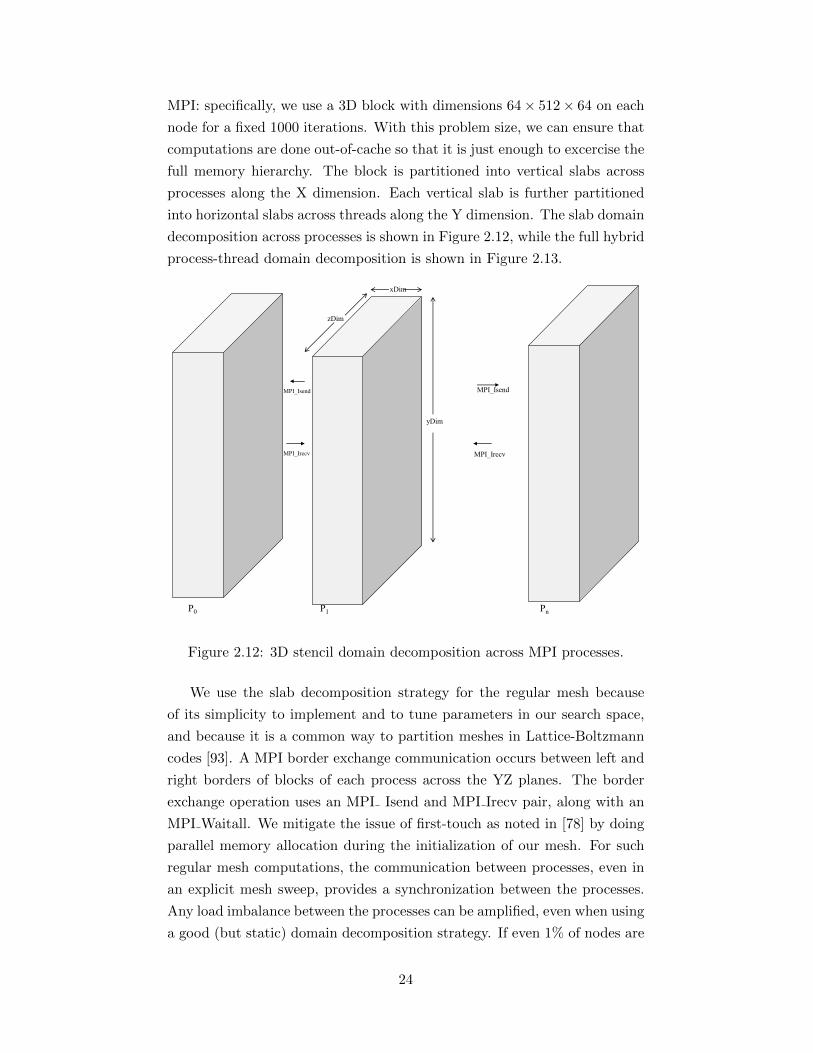
Figure 2.15 and 2.16 shows the domain decomposition for a 3D stencil,
with the dynamic scheduling and locality-aware scheduling srategy applied,
respectively.
Figure 2.17 shows the domain decomposition for a 3D stencil, with our
mixed static/dynamic scheduling strategy applied to the 3D stencil.
Through our experimental studies of tuning our dynamic scheduling
strategy, we pose the following questions:
25
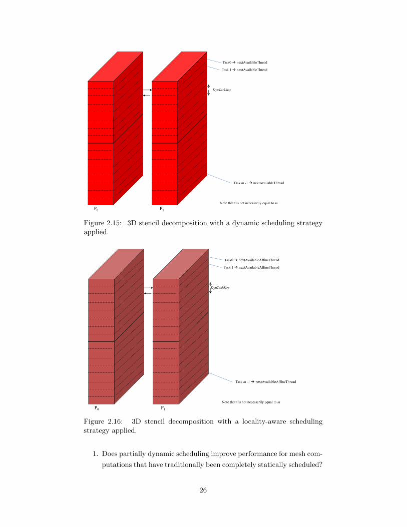
100% dynamic (r =1.0)
P0 P1
Task0 Æ nextAvailableThread
Task 1 Æ nextAvailableThread
DynTaskSize
Task m -1 Æ nextAvailableThread
Note that t is not necessarily equal to m
Figure 2.15: 3D stencil decomposition with a dynamic scheduling strategyapplied. 100% dynamic + Locality
P0 P1
Task0 Æ nextAvailableAffineThread
Task 1 Æ nextAvailableAffineThread
DynTaskSize
Task m -1 Æ nextAvailableAffineThread
Note that t is not necessarily equal to m
Figure 2.16: 3D stencil decomposition with a locality-aware schedulingstrategy applied.
1. Does partially dynamic scheduling improve performance for mesh com-
putations that have traditionally been completely statically scheduled?
26
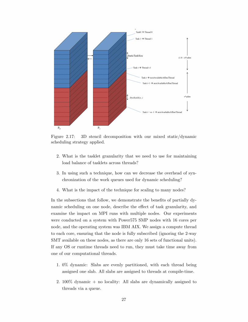
Static + Dynamic
P0 P1
DynTaskSize_i
Task0 Æ Thread 0
Task 1 Æ Thread 1
Task t Æ Thread t-1
StaticTaskSize
Task t Æ nextAvailableAffineThread
Task t + m -1 Æ nextAvailableAffineThread
Task t+1 Æ nextAvailableAffineThread
(1.0 - r)*ydim
r*ydim
Figure 2.17: 3D stencil decomposition with our mixed static/dynamicscheduling strategy applied.
2. What is the tasklet granularity that we need to use for maintaining
load balance of tasklets across threads?
3. In using such a technique, how can we decrease the overhead of syn-
chronization of the work queues used for dynamic scheduling?
4. What is the impact of the technique for scaling to many nodes?
In the subsections that follow, we demonstrate the benefits of partially dy-
namic scheduling on one node, describe the effect of task granularity, and
examine the impact on MPI runs with multiple nodes. Our experiments
were conducted on a system with Power575 SMP nodes with 16 cores per
node, and the operating system was IBM AIX. We assign a compute thread
to each core, ensuring that the node is fully subscribed (ignoring the 2-way
SMT available on these nodes, as there are only 16 sets of functional units).
If any OS or runtime threads need to run, they must take time away from
one of our computational threads.
1. 0% dynamic: Slabs are evenly partitioned, with each thread being
assigned one slab. All slabs are assigned to threads at compile-time.
2. 100% dynamic + no locality: All slabs are dynamically assigned to
threads via a queue.
27
3. 100% dynamic + locality: Same as 2, except that when a thread tries
to dequeue a tasklet, it first searches for tasklets that it last executed
in a previous jacobi iteration.
4. 50% static, 50% dynamic + locality: Each thread first does its static
section, and then immediately starts pulling tasklets from the shared
work queue. This approach is motivated by a desire to reduce overhead
in managing the assignment of tasks to cores.
For the cases involving dynamic scheduling, we initially assume the num-
ber of tasklets in the queue to be 32, and that all threads within an MPI
process share one work queue. Rather than using convergence criteria, we
preset the number of iterations to allow us to verify our results more easily,
and we use 1000 iterations to capture the periodicity of the noise induced
by the system services during a trial [12]. For case 4, i.e., 50% static, 50%
dynamic+locality, locality across timesteps is preserved not just due to the
locality tags, but also (inherently) through the static section assigning the
same set of iterations to threads on all timesteps. Figure 2.18 below shows
the average performance we obtained over 40 trials for each of these cases.
Using static scheduling, the average execution time was about 7 seconds of
wall-clock time. From the figure, we can see that the 50% static, 50% dy-
namic scheduling gives significant performance benefits over the traditional
static scheduling scheduling case. In our 40 trials, we obtained 6 lucky, or
low-noise, runs in the range 6 - 6.5 seconds. The remaining 34 runs were
between 7 - 8 seconds. Using fully dynamic scheduling with no locality,
performance was slightly worse than the statically scheduled case, and for
this case, there were also some small performance variations (within 0.2 sec-
onds) across the 40 trials. Using the 50% dynamic scheduling strategy, the
execution time was 6.53 seconds, giving us over 7% performance gain over
our baseline static scheduling. Thus, using a reasonable partially dynamic
scheduling strategy can reduce performance variation and improve average
performance.
In all cases using dynamic scheduling with locality, thread idle times
(not shown here) contribute to the largest percentage overhead. The high
overhead in case 2 is likely attributed to the fact that threads suffer from
doing work not local to a core. Because some threads suffer coherence cache
misses while others do not, the overall thread idle time, due to threads
waiting at barriers, could be particularly high.
28
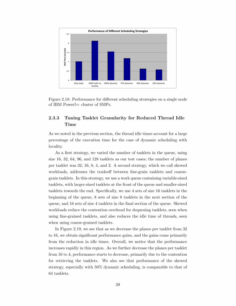
6
6.5
7
7.5
8
8.5
fully sta.c 100% with no locality
100% dynamic 75% dynamic 50% dynamic 25% dynamic
Wall Tim
e (secon
ds)
Performance of Different Scheduling Strategies
Figure 2.18: Performance for different scheduling strategies on a single nodeof IBM Power5+ cluster of SMPs.
2.3.3 Tuning Tasklet Granularity for Reduced Thread Idle
Time
As we noted in the previous section, the thread idle times account for a large
percentage of the execution time for the case of dynamic scheduling with
locality.
As a first strategy, we varied the number of tasklets in the queue, using
size 16, 32, 64, 96, and 128 tasklets as our test cases; the number of planes
per tasklet was 32, 16, 8, 4, and 2. A second strategy, which we call skewed
workloads, addresses the tradeoff between fine-grain tasklets and coarse-
grain tasklets. In this strategy, we use a work queue containing variable-sized
tasklets, with larger-sized tasklets at the front of the queue and smaller-sized
tasklets towards the end. Specifically, we use 4 sets of size 16 tasklets in the
beginning of the queue, 8 sets of size 8 tasklets in the next section of the
queue, and 16 sets of size 4 tasklets in the final section of the queue. Skewed
workloads reduce the contention overhead for dequeuing tasklets, seen when
using fine-grained tasklets, and also reduces the idle time of threads, seen
when using coarse-grained tasklets.
In Figure 2.19, we see that as we decrease the planes per tasklet from 32
to 16, we obtain significant performance gains, and the gains come primarily
from the reduction in idle times. Overall, we notice that the performance
increases rapidly in this region. As we further decrease the planes per tasklet
from 16 to 4, performance starts to decrease, primarily due to the contention
for retrieving the tasklets. We also see that performance of the skewed
strategy, especially with 50% dynamic scheduling, is comparable to that of
64 tasklets.
29
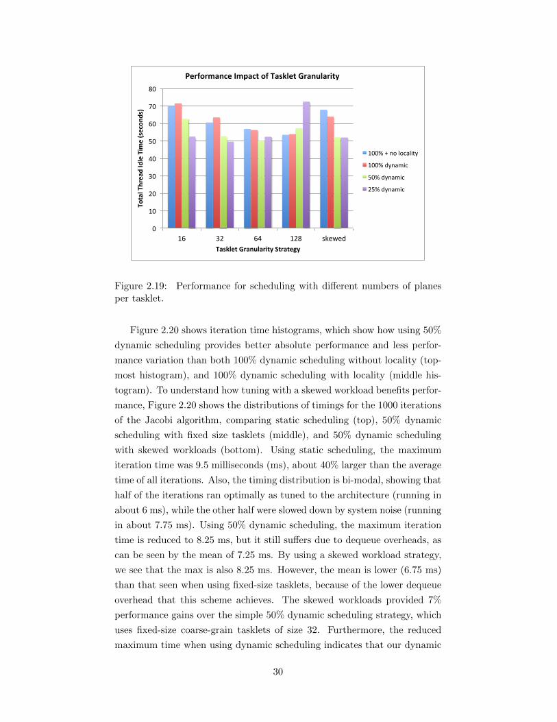
0"
10"
20"
30"
40"
50"
60"
70"
80"
16" 32" 64" 128" skewed"
Total&Thread&Idle&Tim
e&(secon
ds)&
Tasklet&Granularity&Strategy&
Performance&Impact&of&Tasklet&Granularity&
100%"+"no"locality"
100%"dynamic"
50%"dynamic"
25%"dynamic"
Figure 2.19: Performance for scheduling with different numbers of planesper tasklet.
Figure 2.20 shows iteration time histograms, which show how using 50%
dynamic scheduling provides better absolute performance and less perfor-
mance variation than both 100% dynamic scheduling without locality (top-
most histogram), and 100% dynamic scheduling with locality (middle his-
togram). To understand how tuning with a skewed workload benefits perfor-
mance, Figure 2.20 shows the distributions of timings for the 1000 iterations
of the Jacobi algorithm, comparing static scheduling (top), 50% dynamic
scheduling with fixed size tasklets (middle), and 50% dynamic scheduling
with skewed workloads (bottom). Using static scheduling, the maximum
iteration time was 9.5 milliseconds (ms), about 40% larger than the average
time of all iterations. Also, the timing distribution is bi-modal, showing that
half of the iterations ran optimally as tuned to the architecture (running in
about 6 ms), while the other half were slowed down by system noise (running
in about 7.75 ms). Using 50% dynamic scheduling, the maximum iteration
time is reduced to 8.25 ms, but it still suffers due to dequeue overheads, as
can be seen by the mean of 7.25 ms. By using a skewed workload strategy,
we see that the max is also 8.25 ms. However, the mean is lower (6.75 ms)
than that seen when using fixed-size tasklets, because of the lower dequeue
overhead that this scheme achieves. The skewed workloads provided 7%
performance gains over the simple 50% dynamic scheduling strategy, which
uses fixed-size coarse-grain tasklets of size 32. Furthermore, the reduced
maximum time when using dynamic scheduling indicates that our dynamic
30
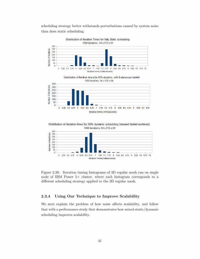
scheduling strategy better withstands perturbations caused by system noise
than does static scheduling.
Figure 2.20: Iteration timing histograms of 3D regular mesh run on singlenode of IBM Power 5+ cluster, where each histogram corresponds to adifferent scheduling strategy applied to the 3D regular mesh.
2.3.4 Using Our Technique to Improve Scalability
We next explain the problem of how noise affects scalability, and follow
that with a performance study that demonstrates how mixed static/dynamic
scheduling improves scalability.
31
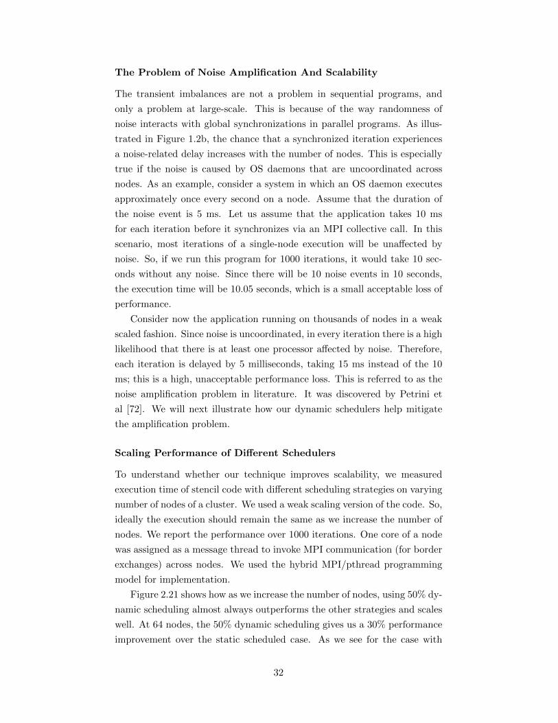
The Problem of Noise Amplification And Scalability
The transient imbalances are not a problem in sequential programs, and
only a problem at large-scale. This is because of the way randomness of
noise interacts with global synchronizations in parallel programs. As illus-
trated in Figure 1.2b, the chance that a synchronized iteration experiences
a noise-related delay increases with the number of nodes. This is especially
true if the noise is caused by OS daemons that are uncoordinated across
nodes. As an example, consider a system in which an OS daemon executes
approximately once every second on a node. Assume that the duration of
the noise event is 5 ms. Let us assume that the application takes 10 ms
for each iteration before it synchronizes via an MPI collective call. In this
scenario, most iterations of a single-node execution will be unaffected by
noise. So, if we run this program for 1000 iterations, it would take 10 sec-
onds without any noise. Since there will be 10 noise events in 10 seconds,
the execution time will be 10.05 seconds, which is a small acceptable loss of
performance.
Consider now the application running on thousands of nodes in a weak
scaled fashion. Since noise is uncoordinated, in every iteration there is a high
likelihood that there is at least one processor affected by noise. Therefore,
each iteration is delayed by 5 milliseconds, taking 15 ms instead of the 10
ms; this is a high, unacceptable performance loss. This is referred to as the
noise amplification problem in literature. It was discovered by Petrini et
al [72]. We will next illustrate how our dynamic schedulers help mitigate
the amplification problem.
Scaling Performance of Different Schedulers
To understand whether our technique improves scalability, we measured
execution time of stencil code with different scheduling strategies on varying
number of nodes of a cluster. We used a weak scaling version of the code. So,
ideally the execution should remain the same as we increase the number of
nodes. We report the performance over 1000 iterations. One core of a node
was assigned as a message thread to invoke MPI communication (for border
exchanges) across nodes. We used the hybrid MPI/pthread programming
model for implementation.
Figure 2.21 shows how as we increase the number of nodes, using 50% dy-
namic scheduling almost always outperforms the other strategies and scales
well. At 64 nodes, the 50% dynamic scheduling gives us a 30% performance
improvement over the static scheduled case. As we see for the case with
32
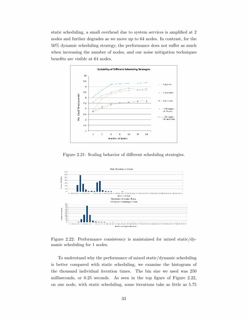
static scheduling, a small overhead due to system services is amplified at 2
nodes and further degrades as we move up to 64 nodes. In contrast, for the
50% dynamic scheduling strategy, the performance does not suffer as much
when increasing the number of nodes, and our noise mitigation techniques
benefits are visible at 64 nodes.
Figure 2.21: Scaling behavior of different scheduling strategies.
Figure 2.22: Performance consistency is maintained for mixed static/dy-namic scheduling for 1 nodes.
To understand why the performance of mixed static/dynamic scheduling
is better compared with static scheduling, we examine the histogram of
the thousand individual iteration times. The bin size we used was 250
milliseconds, or 0.25 seconds. As seen in the top figure of Figure 2.22,
on one node, with static scheduling, some iterations take as little as 5.75
33
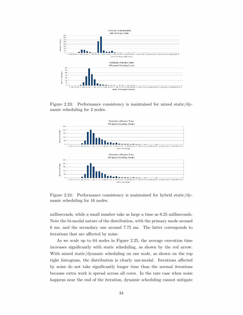
Figure 2.23: Performance consistency is maintained for mixed static/dy-namic scheduling for 2 nodes.
Figure 2.24: Performance consistency is maintained for hybrid static/dy-namic scheduling for 16 nodes.
milliseconds, while a small number take as large a time as 9.25 milliseconds.
Note the bi-modal nature of the distribution, with the primary mode around
6 ms, and the secondary one around 7.75 ms. The latter corresponds to
iterations that are affected by noise.
As we scale up to 64 nodes in Figure 2.25, the average execution time
increases significantly with static scheduling, as shown by the red arrow.
With mixed static/dynamic scheduling on one node, as shown on the top
right histogram, the distribution is clearly uni-modal. Iterations affected
by noise do not take significantly longer time than the normal iterations
because extra work is spread across all cores. In the rare case when noise
happens near the end of the iteration, dynamic scheduling cannot mitigate
34

Figure 2.25: Performance consistency is maintained for hybrid static/dy-namic scheduling for 64 nodes.
its impact, which is why a few iterations take a long time.
The mode is 6.5 ms which is larger than the 6 milliseconds primary
mode for static scheduling because of the overhead of dynamic scheduling,
but much smaller than the secondary mode of static scheduling of 7.75 ms.
Compared to the top histogram of Figure 2.25, the bottom histogram
of Figure 2.25 shows that the distribution has shifted significantly to the
right for static scheduling. This makes sense since each nodes noise event
occurs at different times. The chain of dependencies through MPI messag-
ing for border exchanges compounds the delay across nodes in consecutive
iterations. With dynamic scheduling, the distribution has not shifted as
much. For example, the mode, i.e., the tallest bar of the histogram, only
shifted from 6.75 ms to 7.00 ms. This is because in each iteration, the node
that experiences noise mitigates its effect by scheduling delayed tasklets
to its other threads. Generally, performance variation increases for static
scheduling with increasing numbers of nodes, but is maintained for mixed
static/dynamic scheduling with increasing numbers of nodes.
2.4 Results for Numerical Linear Algebra
Considering the application of our scheduling strategies to the 3D regular
mesh computation in Section 2.2 and Section 2.3, we apply our scheduling
strategies to dense matrix factorization computations, e.g., LU factorization,
QR factorization, Cholesky factorization, a class of numerical linear algebra
computations [89]. Dense matrix factorization computations form an impor-
tant class of numerical linear algebra computations because of their use in
35
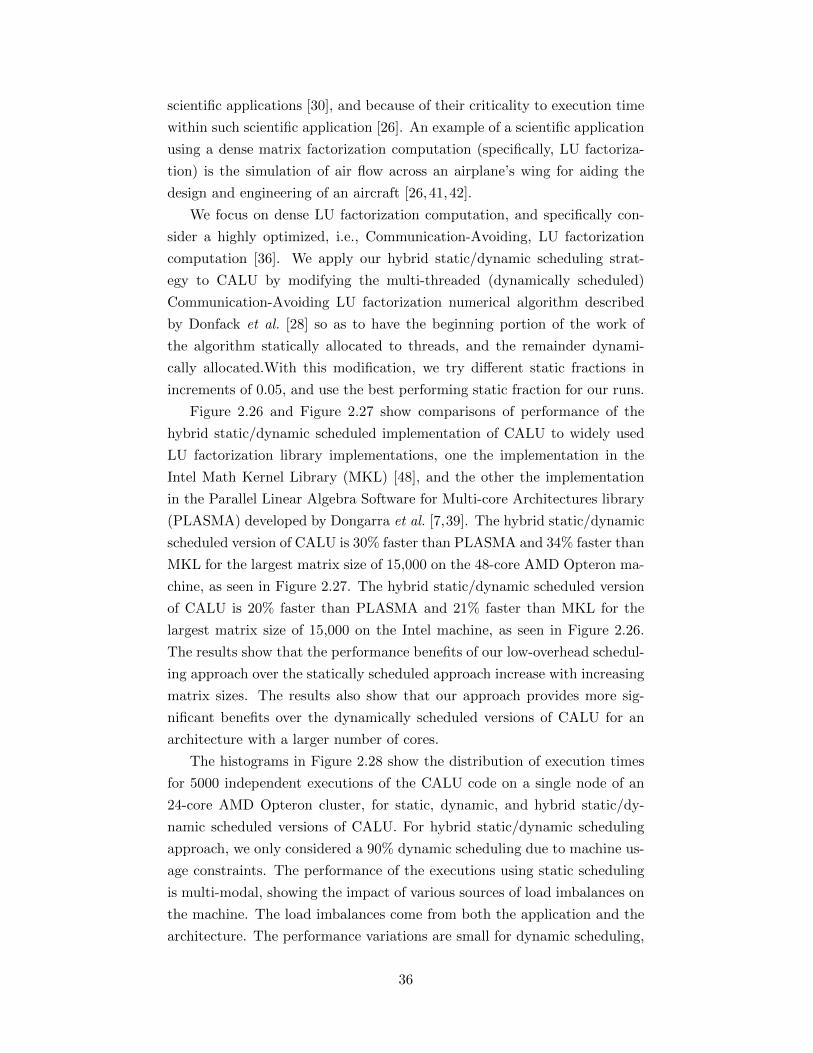
scientific applications [30], and because of their criticality to execution time
within such scientific application [26]. An example of a scientific application
using a dense matrix factorization computation (specifically, LU factoriza-
tion) is the simulation of air flow across an airplane’s wing for aiding the
design and engineering of an aircraft [26,41,42].
We focus on dense LU factorization computation, and specifically con-
sider a highly optimized, i.e., Communication-Avoiding, LU factorization
computation [36]. We apply our hybrid static/dynamic scheduling strat-
egy to CALU by modifying the multi-threaded (dynamically scheduled)
Communication-Avoiding LU factorization numerical algorithm described
by Donfack et al. [28] so as to have the beginning portion of the work of
the algorithm statically allocated to threads, and the remainder dynami-
cally allocated.With this modification, we try different static fractions in
increments of 0.05, and use the best performing static fraction for our runs.
Figure 2.26 and Figure 2.27 show comparisons of performance of the
hybrid static/dynamic scheduled implementation of CALU to widely used
LU factorization library implementations, one the implementation in the
Intel Math Kernel Library (MKL) [48], and the other the implementation
in the Parallel Linear Algebra Software for Multi-core Architectures library
(PLASMA) developed by Dongarra et al. [7,39]. The hybrid static/dynamic
scheduled version of CALU is 30% faster than PLASMA and 34% faster than
MKL for the largest matrix size of 15,000 on the 48-core AMD Opteron ma-
chine, as seen in Figure 2.27. The hybrid static/dynamic scheduled version
of CALU is 20% faster than PLASMA and 21% faster than MKL for the
largest matrix size of 15,000 on the Intel machine, as seen in Figure 2.26.
The results show that the performance benefits of our low-overhead schedul-
ing approach over the statically scheduled approach increase with increasing
matrix sizes. The results also show that our approach provides more sig-
nificant benefits over the dynamically scheduled versions of CALU for an
architecture with a larger number of cores.
The histograms in Figure 2.28 show the distribution of execution times
for 5000 independent executions of the CALU code on a single node of an
24-core AMD Opteron cluster, for static, dynamic, and hybrid static/dy-
namic scheduled versions of CALU. For hybrid static/dynamic scheduling
approach, we only considered a 90% dynamic scheduling due to machine us-
age constraints. The performance of the executions using static scheduling
is multi-modal, showing the impact of various sources of load imbalances on
the machine. The load imbalances come from both the application and the
architecture. The performance variations are small for dynamic scheduling,
36
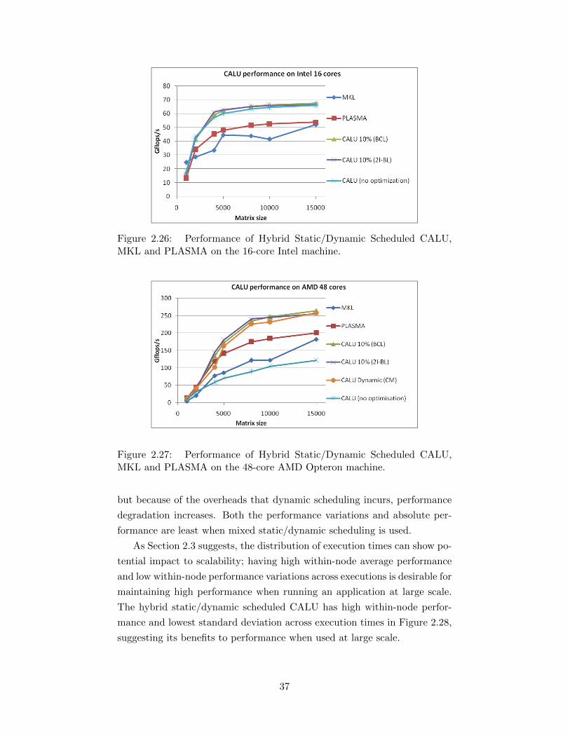
Figure 2.26: Performance of Hybrid Static/Dynamic Scheduled CALU,MKL and PLASMA on the 16-core Intel machine.
Figure 2.27: Performance of Hybrid Static/Dynamic Scheduled CALU,MKL and PLASMA on the 48-core AMD Opteron machine.
but because of the overheads that dynamic scheduling incurs, performance
degradation increases. Both the performance variations and absolute per-
formance are least when mixed static/dynamic scheduling is used.
As Section 2.3 suggests, the distribution of execution times can show po-
tential impact to scalability; having high within-node average performance
and low within-node performance variations across executions is desirable for
maintaining high performance when running an application at large scale.
The hybrid static/dynamic scheduled CALU has high within-node perfor-
mance and lowest standard deviation across execution times in Figure 2.28,
suggesting its benefits to performance when used at large scale.
37
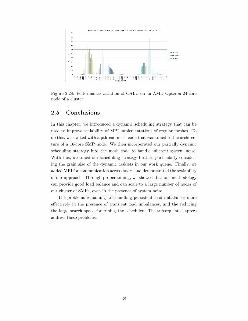
Figure 2.28: Performance variation of CALU on an AMD Opteron 24-corenode of a cluster.
2.5 Conclusions
In this chapter, we introduced a dynamic scheduling strategy that can be
used to improve scalability of MPI implementations of regular meshes. To
do this, we started with a pthread mesh code that was tuned to the architec-
ture of a 16-core SMP node. We then incorporated our partially dynamic
scheduling strategy into the mesh code to handle inherent system noise.
With this, we tuned our scheduling strategy further, particularly consider-
ing the grain size of the dynamic tasklets in our work queue. Finally, we
added MPI for communication across nodes and demonstrated the scalability
of our approach. Through proper tuning, we showed that our methodology
can provide good load balance and can scale to a large number of nodes of
our cluster of SMPs, even in the presence of system noise.
The problems remaining are handling persistent load imbalances more
effectively in the presence of transient load imbalances, and the reducing
the large search space for tuning the scheduler. The subsequent chapters
address these problems.
38
Chapter 3
Weighted Hybrid Scheduling
In the previous chapters, we saw how infrequent uncoordinated noise can
be amplified on synchronous MPI programs running on a large number of
processors. We also developed a hybrid scheduling strategy that combines
both static and dynamic allocation of loop iterations to cores within a node
that handles dynamic load balancing without adding significant overhead.
The nature of noise considered in the last chapter was such that only a small
number of processors/nodes are affected by it in every outer iteration, i.e.,
between MPI synchronizations. This is low-frequency, high-amplitude noise;
by high-amplitude, we mean that the duration of the noise is long enough
to significantly delay the iteration. However, another kind of noise exists:
namely high-frequency, low-amplitude noise. This can arise from short-
duration daemons that execute frequently enough that they affect every
node in each iteration. As we will see, on many platforms, such daemons
run on a fixed subset of cores of each node. From the application’s point of
view, this has the effect of slowing down those cores. Slow cores may also
arise from other architectural factors such as low-priority hardware threads,
e.g., Power7. [91]. We next focus on how to handle such persistent difference
in effective speeds of cores. This chapter is based on material published in
an early paper [52], and so it uses the tasklet-based scheduling technique of
Chapter 2. The tasklet-based scheduling technique described in Chapter 2
is referred to as micro-scheduling in this chapter.
Our key contribution in this chapter is an augmentation of our reac-
tive, queue-based micro-scheduling approach with a form of pro-active load-
balancing. Pro-active load balancing adjusts load before the application
time step begins, while reactive load balancing adjusts load during the time
step. Pro-active load balancers can assign work to each core in proportion
to its availability with respect to OS daemons running on it. We refer to
this augmented load balancing strategy as weighted micro-scheduling.
We show the benefits, over our original solution, for aiding noise mitiga-
tion by:
39
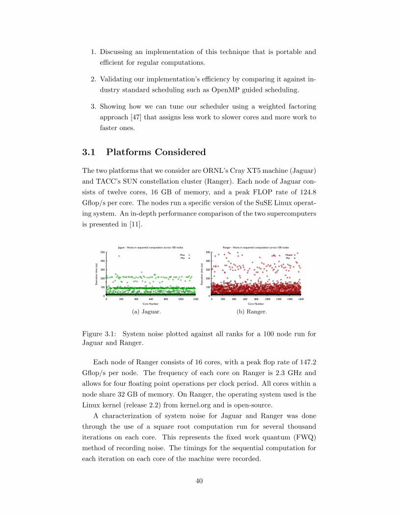
1. Discussing an implementation of this technique that is portable and
efficient for regular computations.
2. Validating our implementation’s efficiency by comparing it against in-
dustry standard scheduling such as OpenMP guided scheduling.
3. Showing how we can tune our scheduler using a weighted factoring
approach [47] that assigns less work to slower cores and more work to
faster ones.
3.1 Platforms Considered
The two platforms that we consider are ORNL’s Cray XT5 machine (Jaguar)
and TACC’s SUN constellation cluster (Ranger). Each node of Jaguar con-
sists of twelve cores, 16 GB of memory, and a peak FLOP rate of 124.8
Gflop/s per core. The nodes run a specific version of the SuSE Linux operat-
ing system. An in-depth performance comparison of the two supercomputers
is presented in [11].
0
100
200
300
400
500
0 200 400 600 800 1000 1200
Exec
utio
n tim
e (u
s)
Core Number
Jaguar - Noise in sequential computation across 100 nodes
MaxMin
(a) Jaguar.
0
100
200
300
400
500
0 200 400 600 800 1000 1200 1400 1600
Exec
utio
n tim
e (u
s)
Core Number
Ranger - Noise in sequential computation across 100 nodes
MaxMin
(b) Ranger.
Figure 3.1: System noise plotted against all ranks for a 100 node run forJaguar and Ranger.
Each node of Ranger consists of 16 cores, with a peak flop rate of 147.2
Gflop/s per node. The frequency of each core on Ranger is 2.3 GHz and
allows for four floating point operations per clock period. All cores within a
node share 32 GB of memory. On Ranger, the operating system used is the
Linux kernel (release 2.2) from kernel.org and is open-source.
A characterization of system noise for Jaguar and Ranger was done
through the use of a square root computation run for several thousand
iterations on each core. This represents the fixed work quantum (FWQ)
method of recording noise. The timings for the sequential computation for
each iteration on each core of the machine were recorded.
40
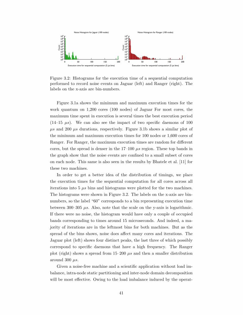
100101102103104105106107108109
0 50 100 150 200C
ount
Execution time for sequential computation (5 µs bins)
Noise Histogram for Jaguar (100 nodes)
100101102103104105106107108109
0 50 100 150 200
Cou
nt
Execution time for sequential computation (5 µs bins)
Noise Histogram for Ranger (100 nodes)
Figure 3.2: Histograms for the execution time of a sequential computationperformed to record noise events on Jaguar (left) and Ranger (right). Thelabels on the x-axis are bin-numbers.
Figure 3.1a shows the minimum and maximum execution times for the
work quantum on 1,200 cores (100 nodes) of Jaguar For most cores, the
maximum time spent in execution is several times the best execution period
(14–15 µs). We can also see the impact of two specific daemons of 100
µs and 200 µs durations, respectively. Figure 3.1b shows a similar plot of
the minimum and maximum execution times for 100 nodes or 1,600 cores of
Ranger. For Ranger, the maximum execution times are random for different
cores, but the spread is denser in the 17–100 µs region. These top bands in
the graph show that the noise events are confined to a small subset of cores
on each node. This same is also seen in the results by Bhatele et al. [11] for
these two machines.
In order to get a better idea of the distribution of timings, we place
the execution times for the sequential computation for all cores across all
iterations into 5 µs bins and histograms were plotted for the two machines.
The histograms were shown in Figure 3.2. The labels on the x-axis are bin-
numbers, so the label “60” corresponds to a bin representing execution time
between 300–305 µs. Also, note that the scale on the y-axis is logarithmic.
If there were no noise, the histogram would have only a couple of occupied
bands corresponding to times around 15 microseconds. And indeed, a ma-
jority of iterations are in the leftmost bins for both machines. But as the
spread of the bins shows, noise does affect many cores and iterations. The
Jaguar plot (left) shows four distinct peaks, the last three of which possibly
correspond to specific daemons that have a high frequency. The Ranger
plot (right) shows a spread from 15–200 µs and then a smaller distribution
around 300 µs.
Given a noise-free machine and a scientific application without load im-
balance, intra-node static partitioning and inter-node domain decomposition
will be most effective. Owing to the load imbalance induced by the operat-
41
ing system, dynamic scheduling can be beneficial to improve performance of
scientific applications [14]. As we saw in Chapter 1, this dynamic schedul-
ing scheme needs to incur low overheads to offer performance benefits for
synchronous MPI applications.
Understanding the characteristics of variations helps us to further fine-
tune the scheduling schemes, which is important to reduce costs of the sched-
uler. Each characteristic of the noise pattern of a platform suggests the im-
portance of a particular feature of our scheduler. In previous chapters, we
designed schedulers to handle the noise pattern where the noise on any given
core is an infrequent event. Within this pattern, there could be several varia-
tions: when a platform has several different noise events of different lengths,
a dynamic scheduling strategy with an assortment of task granularities can
be used; if there are only a few different noise events, each with relatively
similar durations, then we can tune the task granularity.
Yet, none of the scheduling schemes we have developed have used the
noise characteristic of persistence due to core speed variation that is observed
in Figure 3.1a and Figure 3.1b. The next section extends the lightweight
scheduling scheme described in Chapter 2 so that it can mitigate imbalances
due to a mixture of peristent core noise and transient noise, and, as we note
at the end of the chapter, can also be used to handle a mixture including
persistent application imbalance.
3.2 Scheduling Techniques
Locality-sensitive scheduling aims to schedule work on cores that executed
this work in a previous time step. This optimization aims to improve tem-
poral locality, and has been shown to provide benefits in [54].
Our basic scheduler [54] uses a queue to assign chunks of work to cores.
Each queue is implemented as an array of pointers to data structures we call
tasklets. A tasklet is a fine-grained piece of computation that keeps track of
its movement across cores of a node. A queue can consist of an assortment
of tasklets of different lengths. These tasklets are dynamically scheduled
across cores of a node, but are aware of their movement across cores of a
node.
In this work, we improve our technique by augmenting the statically
scheduled stage of the computation with weighted scheduling. Our previous
work assumed that a noise event was equally likely to delay computation of
any core of a node, and that a dynamic scheduler could, in theory, handle
noise events of any duration and any frequency. Yet, short-duration, high
42
frequency events are fine-grained enough that the application quantization
of tasklets limits the ability to distribute the noise across cores evenly. Our
previous work did not handle short-duration, high-frequency noise events
specially.
We address the case when a core is continuously impacted by short-
duration, high-frequency noise events. We observe that a core effectively
becomes “slow” when there are many such OS daemons that are bound
to that particular core and must be frequently time-sliced with the actual
computation. Due to the many different system services that are running on
that core, we observe that the core may have a higher chance of performance
degradation during a time step. Finally, only a subset of cores tend to
have several OS daemons running on them, while the remaining cores are
relatively unoccupied by such system services [72]. If we know that some
cores are always slower than others, we can employ a strategy to offload
some work from the slow cores, and move that work onto faster cores.
Putting both techniques together, we use a prescriptive load balancing
technique in the first stage of the computation to mitigate system noise,
followed by a reactive load balancing technique in the second stage of the
computation. This strategy tries to reduce the amount of work done on
those cores that are heavily occupied by the OS services.
Using weighted scheduling, we obtain performance gains when we are
able to predict which processors likely remain slow throughout the duration
of the application time step. This allows all processors on the node to start
their work at the same time in the subsequent dynamic scheduling stage.
If we know this information before an application time step begins, we can
reduce the chance that the slow core(s) impacts the collective iteration time
across all cores. This can be done by using a form of measurement-based
load balancing as in Charm++ [51].
Weighted scheduling works well because it offloads work proportionally
to the speed of a processor. Its advantage over dynamic scheduling arises
from the fact that it involves no dequeue overheads for locking and unlocking
the work queue. Weighted scheduling tries to ensure that the slow core’s
static section will not be the cause of timestep slowdown. If we do not handle
the slow cores differently, we essentially create a predictable load imbalance.
This will lead to a much higher dynamic fraction, with associated overheads.
This increases the chance that the dynamic load balancing may not be able
to restore balance. In this case, there is no way for the other cores to “steal”
the work from the static section. However, weighted scheduling does also
have its shortcomings. Noise events may not necessarily be restricted to
43

one, or a subset, of the cores on a node. Thus, the predetermined weighted
factoring will serve little purpose. In addition, weighted scheduling does
not handle low-frequency, long-duration noise events. These low-frequency,
long-duration noise events that can happen on any core are seen on both
Jaguar and Ranger, and thus should not be ignored.
The set of cores that are slow varies for different platforms. Even for a
particular platform, the set of cores that are slow can change over the course
of days or weeks. To handle both of these issues, we run an initial loop
with a square-root computation to gather the speeds of each core before the
application begins. We also allow for adjustment of weights during runtime,
to handle the case when the speeds of the cores change during execution of
the program.
Also, for the dynamic scheduling stage, we make use of a more system-
atic auto-tuning methodology to find the best scheduler parameters. The
tuned parameters include the average tasklet granularity and tasklet gran-
ularity distributions. We use a shell script that runs before execution of
the program, to tune the parameters. In the future, we plan to make our
auto-tuning more sophisticated.
3.2.1 Allocating Iterations Based on Weights
We should assign fewer iterations to slower cores, and more iterations to
faster cores. In this section, we describe how to calculate the number of
iterations assigned to each core, based on the history of the computation, i.e.,
of previous outer iterations. For the micro-scheduler described Chapter 2,
recall that the total number of loop iterations was denoted as N , and the
number of cores was p. Given a static fraction fs, the number of iterations
assigned to each core is N ·fsp . Thus, the ith core begins with iteration i ·
N ·fsp . How do we calculate the starting iterations for each core, in terms of
weighted scheduling?
For weighted scheduling, we measure the time taken by static iterations
for each thread, si, with equal allocation as in Chapter 2. The weight for
the ith thread, wi, is calculated as: wi = avg{si}si
. The slower cores which
had a larger value of si have a smaller weight, as we desired. The number
of iterations ki allocated to the ith thread is then given by: ki = wi · fs·Np .
A prefix sum of ki gives the starting iteration for each thread. This needs
to be stored in an array that is calculated at the end of the experimental
uniform allocation phase of the computation. This process of adjustment
can be repeated across outer iterations. In this case, the new ki is calculated
44
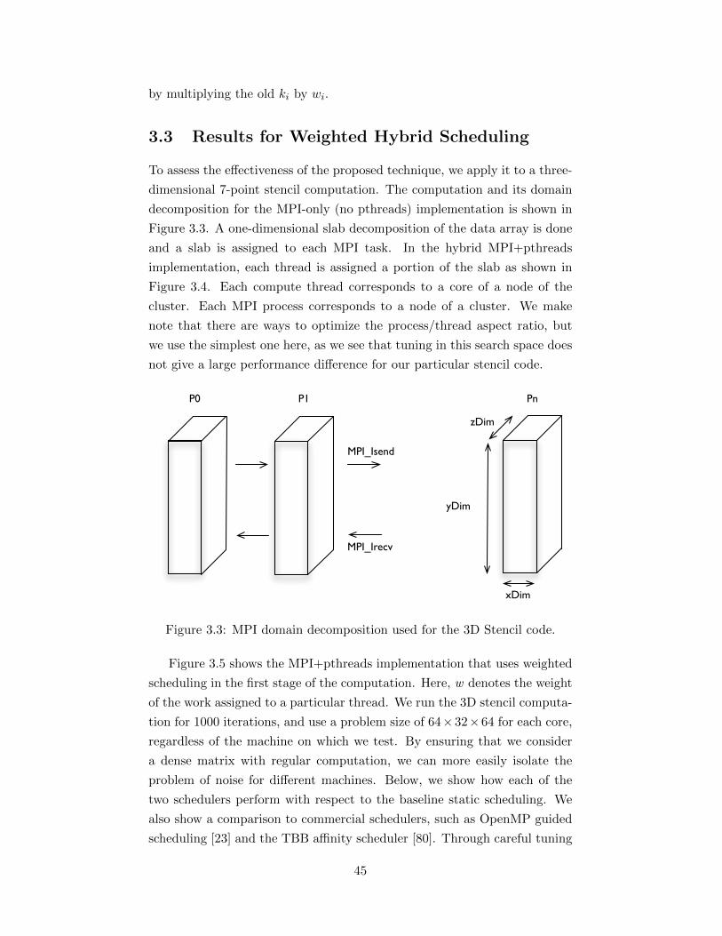
by multiplying the old ki by wi.
3.3 Results for Weighted Hybrid Scheduling
To assess the effectiveness of the proposed technique, we apply it to a three-
dimensional 7-point stencil computation. The computation and its domain
decomposition for the MPI-only (no pthreads) implementation is shown in
Figure 3.3. A one-dimensional slab decomposition of the data array is done
and a slab is assigned to each MPI task. In the hybrid MPI+pthreads
implementation, each thread is assigned a portion of the slab as shown in
Figure 3.4. Each compute thread corresponds to a core of a node of the
cluster. Each MPI process corresponds to a node of a cluster. We make
note that there are ways to optimize the process/thread aspect ratio, but
we use the simplest one here, as we see that tuning in this search space does
not give a large performance difference for our particular stencil code.
xDim
zDim
P0 P1 Pn
MPI_Isend
MPI_Irecv
yDim
Figure 3.3: MPI domain decomposition used for the 3D Stencil code.
Figure 3.5 shows the MPI+pthreads implementation that uses weighted
scheduling in the first stage of the computation. Here, w denotes the weight
of the work assigned to a particular thread. We run the 3D stencil computa-
tion for 1000 iterations, and use a problem size of 64×32×64 for each core,
regardless of the machine on which we test. By ensuring that we consider
a dense matrix with regular computation, we can more easily isolate the
problem of noise for different machines. Below, we show how each of the
two schedulers perform with respect to the baseline static scheduling. We
also show a comparison to commercial schedulers, such as OpenMP guided
scheduling [23] and the TBB affinity scheduler [80]. Through careful tuning
45

xDim
zDim
P0 P1 Pn
MPI_Isend
MPI_Irecv
(1 � fd) · yDim
fd · yDim
Figure 3.4: Hybrid MPI+pthreads domain decomposition with micro-scheduling used for the 3D Stencil code. The dynamic fraction is denotedby fd.
of the parameters shown in Figure 3.5 in our experimentation, we can obtain
significant performance benefits for the stencil application.
xDim
zDim
P0 P1 Pn
MPI_Isend
MPI_Irecv
w1 · (1 � fd) · yDim
p
(1 � fd) · yDim
fd · yDim
w4 · (1 � fd) · yDim
p
Figure 3.5: Hybrid MPI+pthreads domain decomposition used withweighted static and dynamic micro-scheduling for the three-dimensional 7-point stencil computation. The dynamic fraction is denoted by fd, and theweight of thread 1, as shown in this diagram, is denoted by w1.
We now discuss the performance of weighted scheduling, micro-
scheduling, and our combination of the two schedulers, called weighted
micro-scheduling. Figures 3.6 and 3.7 show the performance of the sten-
cil computation described above, using the various schedulers on Jaguar
46
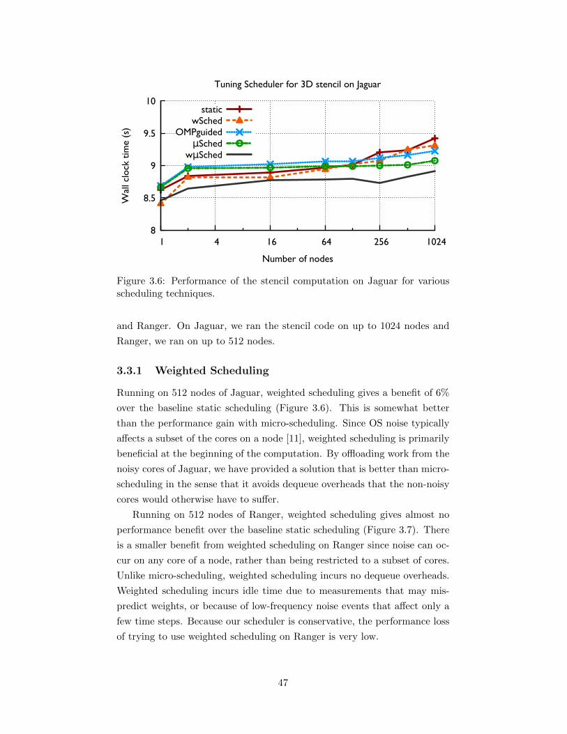
8
8.5
9
9.5
10
1 4 16 64 256 1024
Wal
l clo
ck t
ime
(s)
Number of nodes
Tuning Scheduler for 3D stencil on Jaguar
staticwSched
OMPguidedµSched
wµSched
Figure 3.6: Performance of the stencil computation on Jaguar for variousscheduling techniques.
and Ranger. On Jaguar, we ran the stencil code on up to 1024 nodes and
Ranger, we ran on up to 512 nodes.
3.3.1 Weighted Scheduling
Running on 512 nodes of Jaguar, weighted scheduling gives a benefit of 6%
over the baseline static scheduling (Figure 3.6). This is somewhat better
than the performance gain with micro-scheduling. Since OS noise typically
affects a subset of the cores on a node [11], weighted scheduling is primarily
beneficial at the beginning of the computation. By offloading work from the
noisy cores of Jaguar, we have provided a solution that is better than micro-
scheduling in the sense that it avoids dequeue overheads that the non-noisy
cores would otherwise have to suffer.
Running on 512 nodes of Ranger, weighted scheduling gives almost no
performance benefit over the baseline static scheduling (Figure 3.7). There
is a smaller benefit from weighted scheduling on Ranger since noise can oc-
cur on any core of a node, rather than being restricted to a subset of cores.
Unlike micro-scheduling, weighted scheduling incurs no dequeue overheads.
Weighted scheduling incurs idle time due to measurements that may mis-
predict weights, or because of low-frequency noise events that affect only a
few time steps. Because our scheduler is conservative, the performance loss
of trying to use weighted scheduling on Ranger is very low.
47
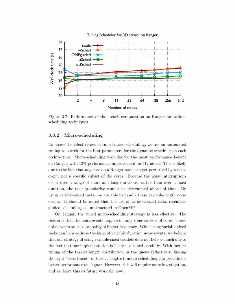
20
22
24
26
28
30
32
34
1 2 4 8 16 32 64 128 256 512
Wal
l clo
ck t
ime
(s)
Number of nodes
Tuning Scheduler for 3D stencil on Ranger
staticwSched
OMPguidedµSched
wµSched
Figure 3.7: Performance of the stencil computation on Ranger for variousscheduling techniques.
3.3.2 Micro-scheduling
To assess the effectiveness of tuned micro-scheduling, we use an automated
tuning to search for the best parameters for the dynamic scheduler on each
architecture. Micro-scheduling provides for the most performance benefit
on Ranger, with 12% performance improvement on 512 nodes. This is likely
due to the fact that any core on a Ranger node can get perturbed by a noise
event, not a specific subset of the cores. Because the noise interruptions
occur over a range of short and long durations, rather than over a fixed
duration, the task granularity cannot be determined ahead of time. By
using variable-sized tasks, we are able to handle these variable-length noise
events. It should be noted that the use of variable-sized tasks resembles
guided scheduling, as implemented in OpenMP.
On Jaguar, the tuned micro-scheduling strategy is less effective. The
reason is that the noise events happen on only some subsets of cores. These
noise events are also probably of higher frequency. While using variable sized
tasks can help address the issue of variable duration noise events, we believe
that our strategy of using variable-sized tasklets does not help as much due to
the fact that our implementation is likely not tuned carefully. With further
tuning of the tasklet length distribution in the queue (effectively, finding
the right “assortment” of tasklet lengths), micro-scheduling can provide for
better performance on Jaguar. However, this will require more investigation,
and we leave this as future work for now.
48
3.3.3 Weighted micro-scheduling
As the preceding sections show, noise that occurs sporadically on any core
of a node can be mitigated by micro-scheduling, and noise that is restricted
to run on a subset of nodes is well-mitigated by weighted scheduling. How-
ever, in practice, production HPC clusters may not have a clear distinction
between the case of noise being focused on a subset of the cores versus the
case where noise occurs sporadically on any core of a node [72].
For example, noise events on a production HPC cluster may be more
likely (rather than restricted) to occur on one core than the other. Thus,
using either of the schedulers in isolation does not necessarily provide for
significant performance gains. To what extent can we combine these two dif-
ferent schedulers to get the best of both worlds? We now discuss the results
obtained when we combine the weighted scheduler and micro-scheduler.
On Jaguar, we observe that noise happens on some cores more than
others. Specifically, cores 0, 6, and 9 are slowest. This is 3 out of the 12 cores
that could potentially finish late and cause a slowdown. By using weighted
micro-scheduling on 512 nodes of Jaguar, we get a performance improvement
of 12% over the baseline static scheduling. This is significantly better than
the performance that we get with using the weighted scheduler (7%) or
the micro-scheduler (9%). In this case, the knowledge that these cores are
noisy allows us to reduce the time for each time step. In addition, dynamic
scheduling handles low-frequency, small duration noise events occurring on
any core.
On 512 nodes of Ranger, weighted micro-scheduling yields a perfor-
mance improvement of 16.6%, which is a slight improvement over the
14.1% improvement we get with just micro-scheduling. All cores are al-
most equally noisy, although core 0 has slightly more noise than other cores.
Weighted scheduling (offloading work from core 0) does help to mitigate
high-frequency, short duration noise on core 0. However, the benefit from
weighted scheduling is still not significant; the benefits obtained through
micro-scheduling still dominate in the results for Ranger.
A key observation we make here is that while weighted scheduling is
not very successful on Ranger, our combined weighted micro-scheduler also
does not hinder performance, compared to the corresponding results for
the weighted scheduler or micro-scheduler. Thus, our solution of combining
weighted and micro-scheduling is portable; when we do not have “slow” cores
on a node, the weighted scheduling portion of the combined weighted micro-
scheduler does not induce unnecessary overhead. Further, our scheduler
49
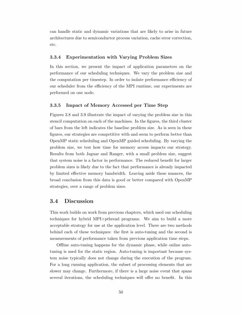
can handle static and dynamic variations that are likely to arise in future
architectures due to semiconductor process variation, cache error correction,
etc.
3.3.4 Experimentation with Varying Problem Sizes
In this section, we present the impact of application parameters on the
performance of our scheduling techniques. We vary the problem size and
the computation per timestep. In order to isolate performance efficiency of
our scheduler from the efficiency of the MPI runtime, our experiments are
performed on one node.
3.3.5 Impact of Memory Accessed per Time Step
Figures 3.8 and 3.9 illustrate the impact of varying the problem size in this
stencil computation on each of the machines. In the figures, the third cluster
of bars from the left indicates the baseline problem size. As is seen in these
figures, our strategies are competitive with and seem to perform better than
OpenMP static scheduling and OpenMP guided scheduling. By varying the
problem size, we test how time for memory access impacts our strategy.
Results from both Jaguar and Ranger, with a small problem size, suggest
that system noise is a factor in performance. The reduced benefit for larger
problem sizes is likely due to the fact that performance is already impacted
by limited effective memory bandwidth. Leaving aside these nuances, the
broad conclusion from this data is good or better compared with OpenMP
strategies, over a range of problem sizes.
3.4 Discussion
This work builds on work from previous chapters, which used our scheduling
techniques for hybrid MPI+pthread programs. We aim to build a more
acceptable strategy for use at the application level. There are two methods
behind each of these techniques: the first is auto-tuning and the second is
measurements of performance taken from previous application time steps.
Offline auto-tuning happens for the dynamic phase, while online auto-
tuning is used for the static region. Auto-tuning is important because sys-
tem noise typically does not change during the execution of the program.
For a long running application, the subset of processing elements that are
slower may change. Furthermore, if there is a large noise event that spans
several iterations, the scheduling techniques will offer no benefit. In this
50
1
10
100
16x384x16 32x384x32 64x384x64 128x384x128
Ave
rage
iter
atio
n tim
e (s
)
Size of stencil
Impact of problem size (Jaguar)
staticµSched
wµSchedOMPguided
Figure 3.8: Impact of problem size on Jaguar for 3D Stencil with differentload balancing strategies.
case, we need a measurement-based load balancing technique such as in
Charm++ [51] that adaptively adjusts to situations where cores are con-
stantly slowed down by operating system events, even across time steps.
We must move work away from those “slow” processing elements.
There is no proactive load measurement involved in our solution of
weighted scheduling. An intelligent load balancer like that in Charm++
uses sophisticated techniques to implement load balancing strategies by col-
lecting load balancing information from previous iterations [10,57,94]. The
nature of load imbalances our strategies are designed to deal with is not
predictable. However, if we can find a pattern in the noise events, an intel-
ligent measurement-based technique that uses periodic load balancing may
be advantageous. Further, our technique can be used in conjunction with
Charm++’s measurement-based load balancers.
Finally, performance tuning a scheduler for a given operating system
is a difficult task. If applications are sensitive to the operating system on
which they are running, the argument for portable application code is further
justified. The rapid pace of innovation of computer architectures is clearly
evident, and can change over just a year’s notice. This requires one to re-tune
application codes continually for these new architectures. Unlike the pace
of innovation for architectures, an operating system can change underneath
within weeks. Furthermore, operating systems are programmed by humans.
This further adds complications because humans make mistakes, thereby
51

1
10
100
16x512x16 32x512x32 64x512x64 128x512x128
Ave
rage
iter
atio
n tim
e (s
)
Size of stencil
Impact of problem size (Ranger)
staticµSched
wµSchedOMPguided
Figure 3.9: Impact of problem size on Ranger for 3D Stencil with differentload balancing strategies.
causing performance (or correctness) bugs in kernel software. Therefore,
strategies such as that described in this chapter that automatically adapt
to variabilities, are desirable.
52

Chapter 4
Slack-Conscious HybridStatic/Dynamic Scheduling
Consider again the basic hybrid scheduling approach that we developed in
Chapter 2. By combining static and dynamic scheduling, we were able to
control overhead while providing dynamic load balancing. We saw that it
is necessary to reduce the dynamic fraction, and therefore the number of
dynamically scheduled iterations to the minimum value that is adequate to
contain the load imbalance. The method that we used for finding this value
of the dynamic fraction was an exhaustive enumerative search. Further,
once the dynamic fraction was decided, the same dynamic fraction was used
on all nodes.
In this chapter, we first develop a model-based method to determine the
dynamic fraction; an empirical search can still be performed near the optimal
dynamic fraction determined by the model. Next, we explore the following
question: If we allow the dynamic fraction to be different on different nodes,
can the dynamic fraction be further reduced, along with reducing the over-
head associated with dynamic scheduling? What we need is a technique
that uses minimally dynamic scheduling on a node, minimizing delay added
to the critical path due to either noise or overhead. As we demonstrate, in
hybrid parallel applications, the mixture of static and dynamic work that
minimizes the average-case runtime varies by each threaded region as well
as by node. Specifically, we show that the percentage of dynamic work that
minimizes the average-case runtime for a threaded computation region in a
noisy system depends on each node’s communication deadline.
The main contributions of this work are:
• A model-based determination of scheduler parameters based on noise,
scheduler overhead and the communication deadline;
• A minimally dynamic scheduling policy that minimizes the average-
case runtime of noisy hybrid applications;
• A tuning technique that enables the above scheduling policy by cou-
pling shared memory and distributed runtimes;
53
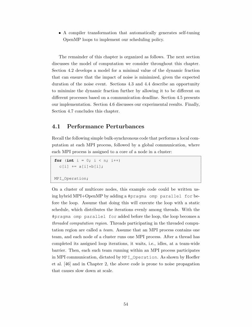
• A compiler transformation that automatically generates self-tuning
OpenMP loops to implement our scheduling policy.
The remainder of this chapter is organized as follows. The next section
discusses the model of computation we consider throughout this chapter.
Section 4.2 develops a model for a minimal value of the dynamic fraction
that can ensure that the impact of noise is minimized, given the expected
duration of the noise event. Sections 4.3 and 4.4 describe an opportunity
to minimize the dynamic fraction further by allowing it to be different on
different processes based on a communication deadline. Section 4.5 presents
our implementation. Section 4.6 discusses our experimental results. Finally,
Section 4.7 concludes this chapter.
4.1 Performance Perturbances
Recall the following simple bulk-synchronous code that performs a local com-
putation at each MPI process, followed by a global communication, where
each MPI process is assigned to a core of a node in a cluster:
for (int i = 0; i < n; i++)
c[i] += a[i]*b[i];
MPI_Operation;
On a cluster of multicore nodes, this example code could be written us-
ing hybrid MPI+OpenMP by adding a #pragma omp parallel for be-
fore the loop. Assume that doing this will execute the loop with a static
schedule, which distributes the iterations evenly among threads. With the
#pragma omp parallel for added before the loop, the loop becomes a
threaded computation region. Threads participating in the threaded compu-
tation region are called a team. Assume that an MPI process contains one
team, and each node of a cluster runs one MPI process. After a thread has
completed its assigned loop iterations, it waits, i.e., idles, at a team-wide
barrier. Then, each such team running within an MPI process participates
in MPI communication, dictated by MPI_Operation. As shown by Hoefler
et al. [46] and in Chapter 2, the above code is prone to noise propagation
that causes slow down at scale.
54
4.2 Model-Based Determination of Minimal
Dynamic Fraction
We now establish the theoretical foundations for our technique which
builds on hybrid scheduling. We assume that applications execute bulk-
synchronously, as computation phases followed by communication phases.
We refer to each bulk-synchronous step as a timestep, and we refer to an
iteration as one unit of work in an OpenMP loop.
We use a simple model for noise, computation, and the fraction of dy-
namic work used. We denote t1 as the duration of a single iteration of a loop,
on one core. We denote the total execution time of a single bulk-synchronous
step, consisting of N loop iterations on p cores, as Tp. We denote the ex-
pected noise delay as δ. We define the portion of dynamically scheduled
work done in a threaded computation region as the dynamic fraction, and
denote it as fd. The portion of statically scheduled work in a threaded com-
putation region is the static fraction, and we define it as 1.0− fd. Table 4.3
provides an overview of all parameters used in the following analysis.
At sufficient scale, noise of length δ occurs with virtual certainty within
each timestep. In principle, at least one process in the job will be affected
by noise with duration δ during each threaded computation region. When
this noise impacts some particular node during a timestep, the noise can
occur on any of the cores of that node. We assume in our model that for
the node that is impacted by noise during an outer iteration, only one core
within that node suffers the noise event.
4.2.1 Using a Model for Hybrid Scheduling
In the absence of dynamic scheduling, when noise occurs on a core, the
critical path will be delayed by δ time units (see Figure 4.2). Therefore,
making at least δ time units worth of work dynamic will allow other cores
to absorb the delayed work to minimize the critical path delay on this node.
Since each thread has Nt1p amount of computation, the relationship between
the delay and dynamic work can be expressed as:
fdNt1p≥ δ (4.1)
fd ≥pδ
Nt1(4.2)
Although the above is an inequality, increasing the dynamic fraction
further does not improve performance. Thus, to achieve our goal of using the
55

Model outputs
fd Fraction of work scheduled dynamically
f ′d Fraction of work scheduled dynamically,reduced for slack
Model inputs
q Overhead of dequeueing single iteration
δ Expected noise duration
δi Expected noise duration on node i
Tp Execution time on p cores with fully static scheduling andno noise
N Total number of iterations across all threads
Change quantities
∆f Change in dynamic fraction
∆η Change in execution time of computation region
τ Sequential time for dynamic work moved
Other variables
t1 Duration of one loop iteration on one thread (running onone core)
d Duration of one dynamic iteration on onethread
η Compute delay due to noise and scheduling overhead
αi Delay added to the critical path by node i
Table 4.1: Overview of all model parameters.
minimal amount of dynamic scheduling, we consider the above relationship
as an equality throughout the remainder of the section.
A minor variant of this model is described in [54] for understanding the
experimental data, but is not used as a part of a runtime strategy for pro-
ducing the results, and was not connected to the experiments. Furthermore,
even if we did attempt to use this model by itself for applications, this model
is overly simplistic. To begin with, it assumes that dynamic scheduling is
free, i.e., that no queueing overhead exists.
With dequeue overhead, each dynamically scheduled iteration takes
slightly longer than a statically scheduled iteration. So, we should use
slightly fewer dynamic tasks to absorb the same amount of noise. Let d
represent the execution time of one dynamically scheduled iteration, p be
the number of cores, and let q represent the scheduler queueing overhead of
a single iteration. Given t1 and q, d can be approximated as:
d = t1 + q (4.3)
We want to use just enough dynamic scheduling so that the scheduler can
parallelize any work displaced by a noise event of length δ. On any one
56
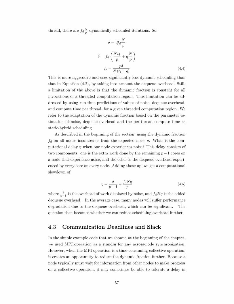
thread, there are fdNp dynamically scheduled iterations. So:
δ = dfdN
p
δ = fd
(Nt1p
+ qN
p
)fd =
pδ
N (t1 + q)(4.4)
This is more aggressive and uses significantly less dynamic scheduling than
that in Equation (4.2), by taking into account the dequeue overhead. Still,
a limitation of the above is that the dynamic fraction is constant for all
invocations of a threaded computation region. This limitation can be ad-
dressed by using run-time predictions of values of noise, dequeue overhead,
and compute time per thread, for a given threaded computation region. We
refer to the adaptation of the dynamic fraction based on the parameter es-
timation of noise, dequeue overhead and the per-thread compute time as
static-hybrid scheduling.
As described in the beginning of the section, using the dynamic fraction
fd on all nodes insulates us from the expected noise δ. What is the com-
putational delay η when one node experiences noise? This delay consists of
two components: one is the extra work done by the remaining p−1 cores on
a node that experience noise, and the other is the dequeue overhead experi-
enced by every core on every node. Adding those up, we get a computational
slowdown of:
η =δ
p− 1+fdNq
p(4.5)
where δp−1 is the overhead of work displaced by noise, and fdNq is the added
dequeue overhead. In the average case, many nodes will suffer performance
degradation due to the dequeue overhead, which can be significant. The
question then becomes whether we can reduce scheduling overhead further.
4.3 Communication Deadlines and Slack
In the simple example code that we showed at the beginning of the chapter,
we used MPI operation as a standin for any across-node synchronization.
However, when the MPI operation is a time-consuming collective operation,
it creates an opportunity to reduce the dynamic fraction further. Because a
node typically must wait for information from other nodes to make progress
on a collective operation, it may sometimes be able to tolerate a delay in
57
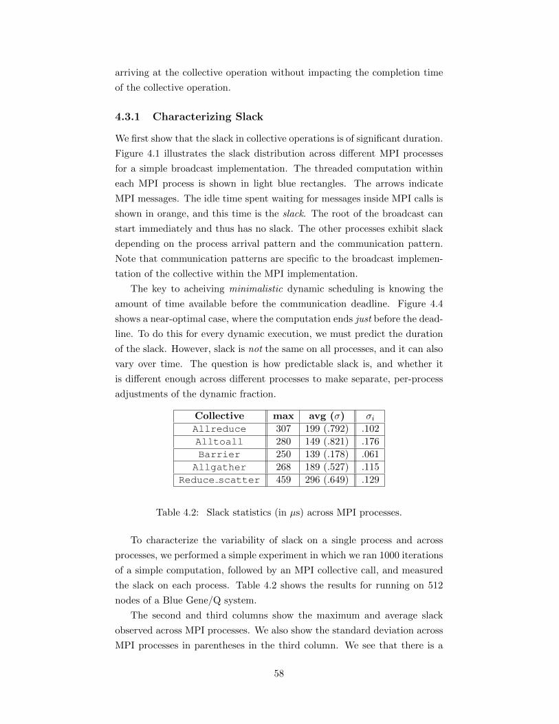
arriving at the collective operation without impacting the completion time
of the collective operation.
4.3.1 Characterizing Slack
We first show that the slack in collective operations is of significant duration.
Figure 4.1 illustrates the slack distribution across different MPI processes
for a simple broadcast implementation. The threaded computation within
each MPI process is shown in light blue rectangles. The arrows indicate
MPI messages. The idle time spent waiting for messages inside MPI calls is
shown in orange, and this time is the slack. The root of the broadcast can
start immediately and thus has no slack. The other processes exhibit slack
depending on the process arrival pattern and the communication pattern.
Note that communication patterns are specific to the broadcast implemen-
tation of the collective within the MPI implementation.
The key to acheiving minimalistic dynamic scheduling is knowing the
amount of time available before the communication deadline. Figure 4.4
shows a near-optimal case, where the computation ends just before the dead-
line. To do this for every dynamic execution, we must predict the duration
of the slack. However, slack is not the same on all processes, and it can also
vary over time. The question is how predictable slack is, and whether it
is different enough across different processes to make separate, per-process
adjustments of the dynamic fraction.
Collective max avg (σ) σiAllreduce 307 199 (.792) .102
Alltoall 280 149 (.821) .176
Barrier 250 139 (.178) .061
Allgather 268 189 (.527) .115
Reduce scatter 459 296 (.649) .129
Table 4.2: Slack statistics (in µs) across MPI processes.
To characterize the variability of slack on a single process and across
processes, we performed a simple experiment in which we ran 1000 iterations
of a simple computation, followed by an MPI collective call, and measured
the slack on each process. Table 4.2 shows the results for running on 512
nodes of a Blue Gene/Q system.
The second and third columns show the maximum and average slack
observed across MPI processes. We also show the standard deviation across
MPI processes in parentheses in the third column. We see that there is a
58
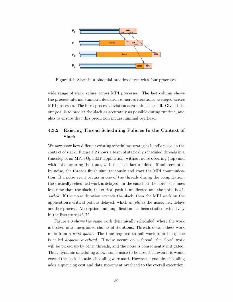
P0
P1
P2
P3
MPI
MPI
Slack MPI
MPISend Send
Send
Recv
Recv
Recv
Slack
Slack
Figure 4.1: Slack in a binomial broadcast tree with four processes.
wide range of slack values across MPI processes. The last column shows
the process-internal standard deviation σi across iterations, averaged across
MPI processes. The intra-process deviation across time is small. Given this,
our goal is to predict the slack as accurately as possible during runtime, and
also to ensure that this prediction incurs minimal overhead.
4.3.2 Existing Thread Scheduling Policies In the Context of
Slack
We now show how different existing scheduling strategies handle noise, in the
context of slack. Figure 4.2 shows a team of statically scheduled threads in a
timestep of an MPI+OpenMP application, without noise occuring (top) and
with noise occuring (bottom), with the slack factor added. If uninterrupted
by noise, the threads finish simultaneously and start the MPI communica-
tion. If a noise event occurs in one of the threads during the computation,
the statically scheduled work is delayed. In the case that the noise consumes
less time than the slack, the critical path is unaffected and the noise is ab-
sorbed. If the noise duration exceeds the slack, then the MPI work on the
application’s critical path is delayed, which amplifies the noise, i.e., delays
another process. Absorption and amplification has been studied extensively
in the literature [46,72].
Figure 4.3 shows the same work dynamically scheduled, where the work
is broken into fine-grained chunks of iterations. Threads obtain these work
units from a work queue. The time required to pull work from the queue
is called dequeue overhead. If noise occurs on a thread, the “lost” work
will be picked up by other threads, and the noise is consequently mitigated.
Thus, dynamic scheduling allows some noise to be absorbed even if it would
exceed the slack if static scheduling were used. However, dynamic scheduling
adds a queueing cost and data movement overhead to the overall execution.
59
Slack MPI
1234
1234
Time
Amplification
Noise
ThreadsThreads
MPI
Tp S
Figure 4.2: Impact of performance irregularities for static scheduling, withslack factor added.
1234
Time
1234
Noise
Delay
Slack
ThreadsThreads
MPI
MPI
Amplification
t1q
S
Figure 4.3: Resilience to performance irregularities with dynamic scheduling,with slack factor added.
The overhead caused by this cost depends crucially on the granularity of
the work, but can be significant for loops typically found in computational
science applications [27,54].
To reduce queueing cost, we can schedule a large fraction of the itera-
tions statically and schedule only a minimal number of iterations dynami-
cally. We call this mechanism Hybrid Static/Dynamic Scheduling, or Hybrid
Scheduling. Figure 4.4 illustrates this technique. Here, only the second part
of the workload is scheduled dynamically. The first part, shown in blue,
is scheduled statically, without any overhead. The noise event causes load
imbalance, but the dynamic scheduling moves excess work off the critical
path. Additionally, the schedule still incurs some dequeue overhead, but
much smaller than that of a fully dynamic scheme. The goal of our ap-
proach is to use just enough dynamic iterations to reschedule work delayed
by noise, while using enough static iterations to prevent the communication
phase from being delayed by queueing overhead.
60
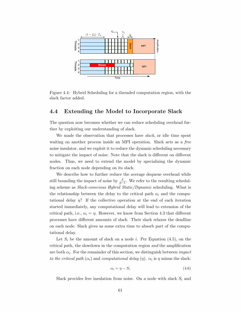
1234
1234
Time
Slack
Noise
ThreadsThreads
MPI
MPI
Amplification
t1q(1 � fd) · Tp S
Figure 4.4: Hybrid Scheduling for a threaded computation region, with theslack factor added.
4.4 Extending the Model to Incorporate Slack
The question now becomes whether we can reduce scheduling overhead fur-
ther by exploiting our understanding of slack.
We made the observation that processes have slack, or idle time spent
waiting on another process inside an MPI operation. Slack acts as a free
noise insulator, and we exploit it to reduce the dynamic scheduling necessary
to mitigate the impact of noise. Note that the slack is different on different
nodes. Thus, we need to extend the model by specializing the dynamic
fraction on each node depending on its slack.
We describe how to further reduce the average dequeue overhead while
still bounding the impact of noise by δp−1 . We refer to the resulting schedul-
ing scheme as Slack-conscious Hybrid Static/Dynamic scheduling. What is
the relationship between the delay to the critical path αi and the compu-
tational delay η? If the collective operation at the end of each iteration
started immediately, any computational delay will lead to extension of the
critical path, i.e., αi = η. However, we know from Section 4.3 that different
processes have different amounts of slack. Their slack relaxes the deadline
on each node. Slack gives us some extra time to absorb part of the compu-
tational delay.
Let Si be the amount of slack on a node i. Per Equation (4.5), on the
critical path, the slowdown in the computation region and the amplification
are both αi. For the remainder of this section, we distinguish between impact
to the critical path (αi) and computational delay (η). αi is η minus the slack:
αi = η − Si (4.6)
Slack provides free insulation from noise. On a node with slack Si and
61
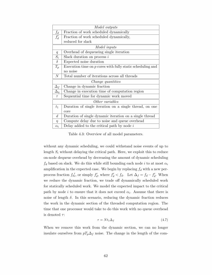
Model outputs
fd Fraction of work scheduled dynamically
f ′d Fraction of work scheduled dynamically,reduced for slack
Model inputs
q Overhead of dequeueing single iteration
Si Slack duration on process i
δ Expected noise duration
Tp Execution time on p cores with fully static scheduling andno noise
N Total number of iterations across all threads
Change quantities
∆f Change in dynamic fraction
∆η Change in execution time of computation region
τ Sequential time for dynamic work moved
Other variables
t1 Duration of single iteration on a single thread, on onecore
d Duration of single dynamic iteration on a single thread
η Compute delay due to noise and queue overhead
αi Delay added to the critical path by node i
Table 4.3: Overview of all model parameters.
without any dynamic scheduling, we could withstand noise events of up to
length Si without delaying the critical path. Here, we exploit this to reduce
on-node dequeue overhead by decreasing the amount of dynamic scheduling
fd based on slack. We do this while still bounding each node i to at most αi
amplification in the expected case. We begin by replacing fd with a new per-
process fraction fd′i, or simply f ′d, where f ′d < fd. Let ∆f = fd− f ′d. When
we reduce the dynamic fraction, we trade off dynamically scheduled work
for statically scheduled work. We model the expected impact to the critical
path by node i to ensure that it does not exceed αi. Assume that there is
noise of length δ. In this scenario, reducing the dynamic fraction reduces
the work in the dynamic section of the threaded computation region. The
time that one processor would take to do this work with no queue overhead
is denoted τ :
τ = Nt1∆f (4.7)
When we remove this work from the dynamic section, we can no longer
insulate ourselves from pTp∆f noise. The change in the length of the com-
62

putation region (η) due to this scheduling change when noise occurs is:
∆η = −τp
+ τ −∆fNq (4.8)
The first two terms model the change in computational load, and the last
term models the change in queuing overhead. Now, we have enough infor-
mation to choose f ′d so that the node’s impact to the critical path is still αi
in the expected case. Let α′i, or simply α′, be the amplification encountered
using f ′d. α′ is equal to amplification using fd plus ∆η, minus the slack:
α′ = α+ ∆η − S (4.9)
Set the above equal to α and solve for fd′:
α = α+ ∆η − S
S = −τp
+ τ −∆fNq
S = −pNt1∆f + Tp∆f + ∆fNq
S = −∆f ((p2 − 1)Nt1 +Nt1p
+Nq)
− S
(p2 − 1)Nt1p +Nq= fd − f ′d
f ′d = fd −S
(p2 − 1)Nt1p −Nq(4.10)
This dynamic fraction will ensure that amplification in the expected
case does not exceed α, i.e., it is no worse than for nodes that are on the
critical path. Indeed, it can be observed trivially that when we are on the
critical path, S = 0 and f ′d = fd. As slack grows, we reduce the dynamic
scheduling used when a node is unaffected by noise. We prefer to use slack
for insulation when it is available because dequeue overhead of dynamic
scheduling can amplify even when there is no noise.
This formulation allows f ′d to be negative when slack is large, but in
reality we cannot use less than 0% dynamic scheduling. We revise Equa-
tion (4.10) to:
f ′d = min
(fd −
S
(p− 1)Nt1p −Nq, 0
)(4.11)
4.5 Slack-Conscious Hybrid Static/Dynamic
Scheduling
The percentage of dynamic work that minimizes the average-case runtime
of a threaded region in a noisy system depends on each node’s communi-
cation deadline. This fact implies that optimizing the performance of a
63
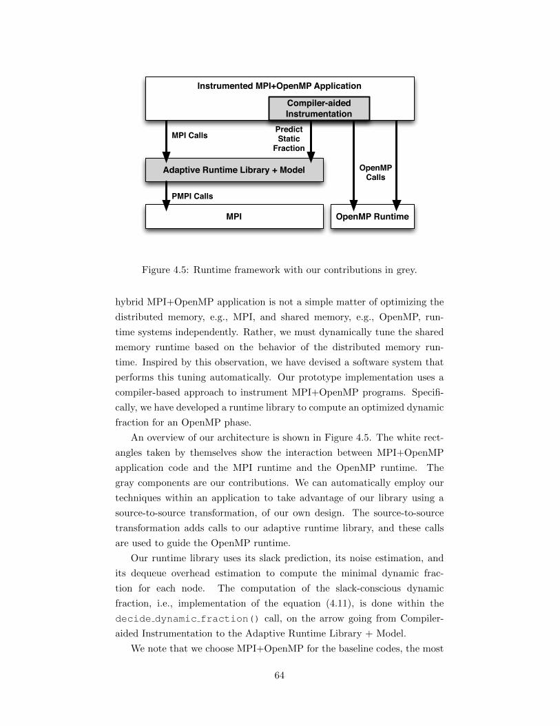
MPI
Adaptive Runtime Library + Model
OpenMP Runtime
OpenMPCalls
PredictStatic
FractionMPI Calls
PMPI Calls
Instrumented MPI+OpenMP Application
Compiler-aidedInstrumentation
Figure 4.5: Runtime framework with our contributions in grey.
hybrid MPI+OpenMP application is not a simple matter of optimizing the
distributed memory, e.g., MPI, and shared memory, e.g., OpenMP, run-
time systems independently. Rather, we must dynamically tune the shared
memory runtime based on the behavior of the distributed memory run-
time. Inspired by this observation, we have devised a software system that
performs this tuning automatically. Our prototype implementation uses a
compiler-based approach to instrument MPI+OpenMP programs. Specifi-
cally, we have developed a runtime library to compute an optimized dynamic
fraction for an OpenMP phase.
An overview of our architecture is shown in Figure 4.5. The white rect-
angles taken by themselves show the interaction between MPI+OpenMP
application code and the MPI runtime and the OpenMP runtime. The
gray components are our contributions. We can automatically employ our
techniques within an application to take advantage of our library using a
source-to-source transformation, of our own design. The source-to-source
transformation adds calls to our adaptive runtime library, and these calls
are used to guide the OpenMP runtime.
Our runtime library uses its slack prediction, its noise estimation, and
its dequeue overhead estimation to compute the minimal dynamic frac-
tion for each node. The computation of the slack-conscious dynamic
fraction, i.e., implementation of the equation (4.11), is done within the
decide dynamic fraction() call, on the arrow going from Compiler-
aided Instrumentation to the Adaptive Runtime Library + Model.
We note that we choose MPI+OpenMP for the baseline codes, the most
64
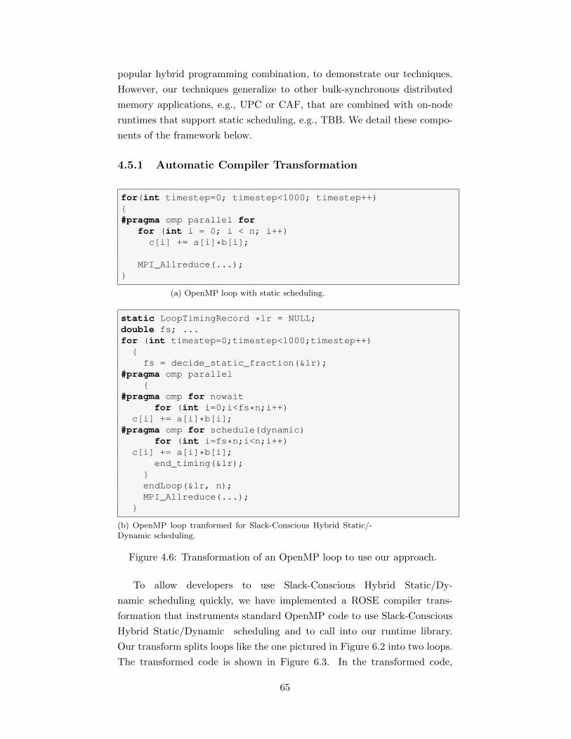
popular hybrid programming combination, to demonstrate our techniques.
However, our techniques generalize to other bulk-synchronous distributed
memory applications, e.g., UPC or CAF, that are combined with on-node
runtimes that support static scheduling, e.g., TBB. We detail these compo-
nents of the framework below.
4.5.1 Automatic Compiler Transformation
for(int timestep=0; timestep<1000; timestep++){#pragma omp parallel for
for (int i = 0; i < n; i++)c[i] += a[i]*b[i];
MPI_Allreduce(...);}
(a) OpenMP loop with static scheduling.
static LoopTimingRecord *lr = NULL;double fs; ...for (int timestep=0;timestep<1000;timestep++)
{fs = decide_static_fraction(&lr);
#pragma omp parallel{
#pragma omp for nowaitfor (int i=0;i<fs*n;i++)
c[i] += a[i]*b[i];#pragma omp for schedule(dynamic)
for (int i=fs*n;i<n;i++)c[i] += a[i]*b[i];
end_timing(&lr);}endLoop(&lr, n);MPI_Allreduce(...);
}
(b) OpenMP loop tranformed for Slack-Conscious Hybrid Static/-Dynamic scheduling.
Figure 4.6: Transformation of an OpenMP loop to use our approach.
To allow developers to use Slack-Conscious Hybrid Static/Dy-
namic scheduling quickly, we have implemented a ROSE compiler trans-
formation that instruments standard OpenMP code to use Slack-Conscious
Hybrid Static/Dynamic scheduling and to call into our runtime library.
Our transform splits loops like the one pictured in Figure 6.2 into two loops.
The transformed code is shown in Figure 6.3. In the transformed code,
65

the first OpenMP loop’s iterations are statically scheduled, and the sec-
ond OpenMP loop’s iterations are dynamically scheduled. The compiler
inserts the nowait clause on the statically scheduled OpenMP loop to al-
low its threads to start the dynamic region immediately, without synchro-
nization. Before the OpenMP region, the ROSE transformation adds the
predict dynamic fraction() call and other instrumentations, the re-
sults of which are used to determine the bounds of our static and dynamic
loops. Our approach relies heavily on cooperation between the MPI and
OpenMP runtimes, and the predict dynamic fraction() call is where
the two communicate. Without this call, OpenMP would be unable to get
the information it needs from MPI to enable Slack-Conscious Hybrid Stat-
ic/Dynamic scheduling.
4.5.2 Runtime Parameter Estimation
Within the predict dynamic fraction() call, observed slack values
and measured parameters of computation time per thread N ·t1p , dequeue
overhead q, and noise length δ are needed to calculate this per-process dy-
namic fraction, as determined in Equation 4.11 in Section 5.2. Below, we
explain how these values are obtained during runtime.
Basic Scheduler Measurements
The record parameter stores the values of N ·t1p , q and δ. The scheduling
overhead q is measured with a dynamically scheduled OpenMP loop at the
initialization of the library. This loop runs multiple dynamically scheduled
short iterations to estimate the dequeue overhead q. The expected noise
event length δ is observed by running multiple measurement iterations in
a tight loop containing within its body a square root calculation. The dif-
ference between the minimum and maximum runtimes is used to estimate
δ. We estimate N ·t1p by obtaining the minimally observed time taken for
the statically scheduled section from previous invocations of the loop. We
obtain t1 by dividing this time by the number of iterations executed by a
thread statically, and use it to calculate N ·t1p .
We denote the time taken in some arbitrary invocation as Tp, and the
time taken for invocation i as Tp,i. The time for executing a single invoca-
tion of a loop depends on the application workload. Thus, we measure it for
each OpenMP parallel loop. The mechanism is shown in Figure 6.3. The
endLoop() function records time taken for the loop of the precedent invo-
cation of the OpenMP region, and we collect the timing for each invocation
66
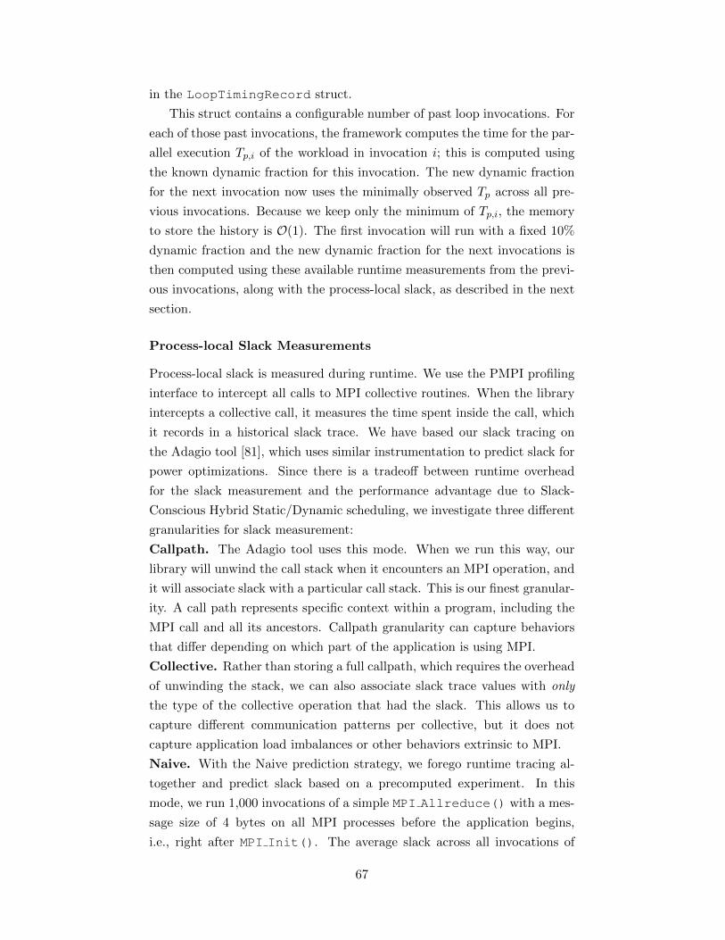
in the LoopTimingRecord struct.
This struct contains a configurable number of past loop invocations. For
each of those past invocations, the framework computes the time for the par-
allel execution Tp,i of the workload in invocation i; this is computed using
the known dynamic fraction for this invocation. The new dynamic fraction
for the next invocation now uses the minimally observed Tp across all pre-
vious invocations. Because we keep only the minimum of Tp,i, the memory
to store the history is O(1). The first invocation will run with a fixed 10%
dynamic fraction and the new dynamic fraction for the next invocations is
then computed using these available runtime measurements from the previ-
ous invocations, along with the process-local slack, as described in the next
section.
Process-local Slack Measurements
Process-local slack is measured during runtime. We use the PMPI profiling
interface to intercept all calls to MPI collective routines. When the library
intercepts a collective call, it measures the time spent inside the call, which
it records in a historical slack trace. We have based our slack tracing on
the Adagio tool [81], which uses similar instrumentation to predict slack for
power optimizations. Since there is a tradeoff between runtime overhead
for the slack measurement and the performance advantage due to Slack-
Conscious Hybrid Static/Dynamic scheduling, we investigate three different
granularities for slack measurement:
Callpath. The Adagio tool uses this mode. When we run this way, our
library will unwind the call stack when it encounters an MPI operation, and
it will associate slack with a particular call stack. This is our finest granular-
ity. A call path represents specific context within a program, including the
MPI call and all its ancestors. Callpath granularity can capture behaviors
that differ depending on which part of the application is using MPI.
Collective. Rather than storing a full callpath, which requires the overhead
of unwinding the stack, we can also associate slack trace values with only
the type of the collective operation that had the slack. This allows us to
capture different communication patterns per collective, but it does not
capture application load imbalances or other behaviors extrinsic to MPI.
Naive. With the Naive prediction strategy, we forego runtime tracing al-
together and predict slack based on a precomputed experiment. In this
mode, we run 1,000 invocations of a simple MPI Allreduce() with a mes-
sage size of 4 bytes on all MPI processes before the application begins,
i.e., right after MPI Init(). The average slack across all invocations of
67
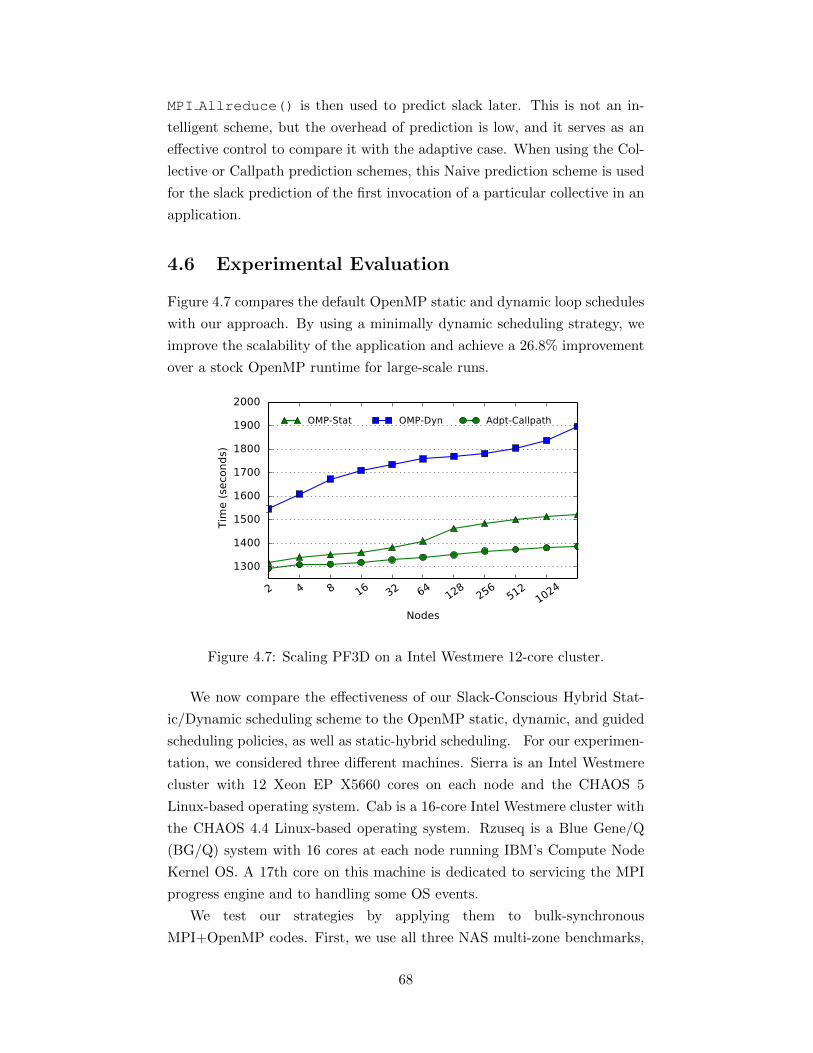
MPI Allreduce() is then used to predict slack later. This is not an in-
telligent scheme, but the overhead of prediction is low, and it serves as an
effective control to compare it with the adaptive case. When using the Col-
lective or Callpath prediction schemes, this Naive prediction scheme is used
for the slack prediction of the first invocation of a particular collective in an
application.
4.6 Experimental Evaluation
Figure 4.7 compares the default OpenMP static and dynamic loop schedules
with our approach. By using a minimally dynamic scheduling strategy, we
improve the scalability of the application and achieve a 26.8% improvement
over a stock OpenMP runtime for large-scale runs.
2 4 8 16 32 64128
256512
1024
Nodes
1300
1400
1500
1600
1700
1800
1900
2000
Tim
e (
seco
nd
s)
OMP-Stat OMP-Dyn Adpt-Callpath
Figure 4.7: Scaling PF3D on a Intel Westmere 12-core cluster.
We now compare the effectiveness of our Slack-Conscious Hybrid Stat-
ic/Dynamic scheduling scheme to the OpenMP static, dynamic, and guided
scheduling policies, as well as static-hybrid scheduling. For our experimen-
tation, we considered three different machines. Sierra is an Intel Westmere
cluster with 12 Xeon EP X5660 cores on each node and the CHAOS 5
Linux-based operating system. Cab is a 16-core Intel Westmere cluster with
the CHAOS 4.4 Linux-based operating system. Rzuseq is a Blue Gene/Q
(BG/Q) system with 16 cores at each node running IBM’s Compute Node
Kernel OS. A 17th core on this machine is dedicated to servicing the MPI
progress engine and to handling some OS events.
We test our strategies by applying them to bulk-synchronous
MPI+OpenMP codes. First, we use all three NAS multi-zone benchmarks,
68
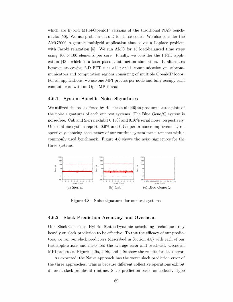
which are hybrid MPI+OpenMP versions of the traditional NAS bench-
marks [50]. We use problem class D for these codes. We also consider the
AMG2006 Algebraic multigrid application that solves a Laplace problem
with Jacobi relaxation [5]. We run AMG for 13 load-balanced time steps
using 100 × 100 elements per core. Finally, we consider the PF3D appli-
cation [43], which is a laser-plasma interaction simulation. It alternates
between successive 2-D FFT MPI Alltoall communication on subcom-
municators and computation regions consisting of multiple OpenMP loops.
For all applications, we use one MPI process per node and fully occupy each
compute core with an OpenMP thread.
4.6.1 System-Specific Noise Signatures
We utilized the tools offered by Hoefler et al. [46] to produce scatter plots of
the noise signatures of each our test systems. The Blue Gene/Q system is
noise-free. Cab and Sierra exhibit 0.18% and 0.16% serial noise, respectively.
Our runtime system reports 0.6% and 0.7% performance improvement, re-
spectively, showing consistency of our runtime system measurements with a
commonly used benchmark. Figure 4.8 shows the noise signatures for the
three systems.
0.01
0.1
1
10
100
1000
10000
0 5 10 15 20 25 30 35 40 45 50
De
tou
r [u
s]
Sample Time [s]
(a) Sierra.
0.01
0.1
1
10
100
1000
10000
0 5 10 15 20 25 30 35 40 45 50
De
tou
r [u
s]
Sample Time [s]
(b) Cab.
0.01
0.1
1
10
100
1000
10000
0 200u 400u 600u 800u 1m 1m 1m 2m 2m
De
tou
r [u
s]
Sample Time [s]
(c) Blue Gene/Q.
Figure 4.8: Noise signatures for our test systems.
4.6.2 Slack Prediction Accuracy and Overhead
Our Slack-Conscious Hybrid Static/Dynamic scheduling techniques rely
heavily on slack prediction to be effective. To test the efficacy of our predic-
tors, we ran our slack predictors (described in Section 4.5) with each of our
test applications and measured the average error and overhead, across all
MPI processes. Figures 4.9a, 4.9b, and 4.9c show the results for slack error.
As expected, the Naive approach has the worst slack prediction error of
the three approaches. This is because different collective operations exhibit
different slack profiles at runtime. Slack prediction based on collective type
69
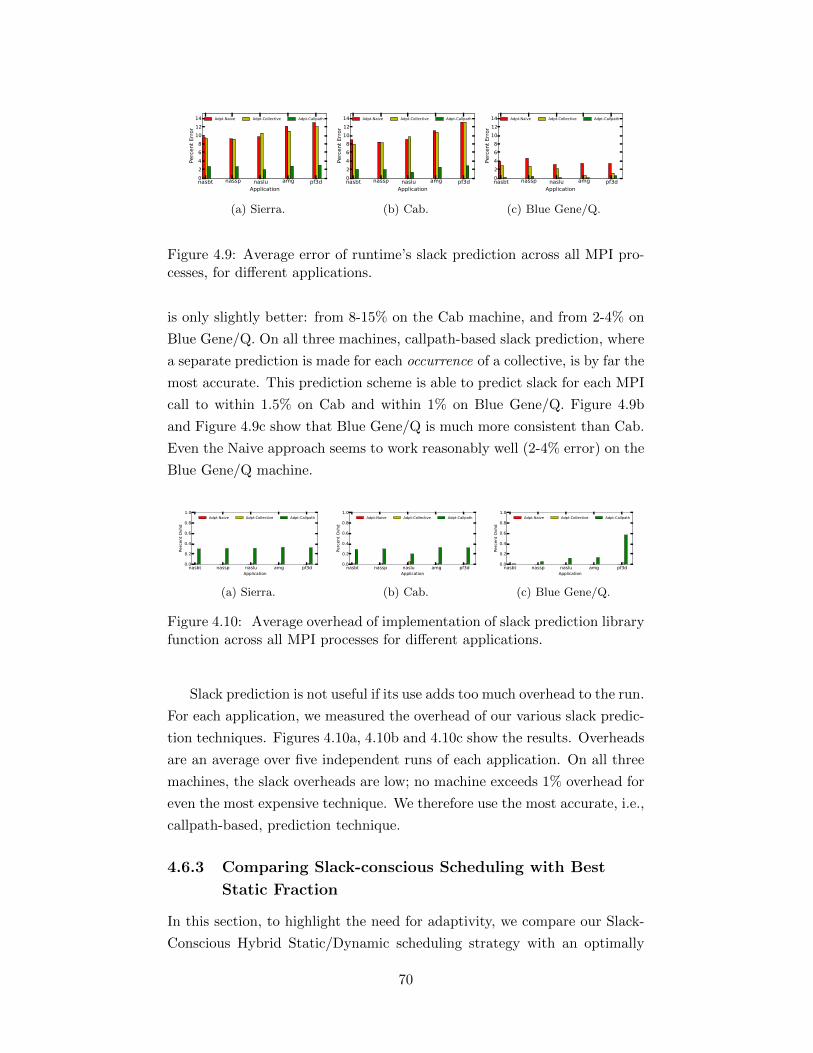
nasbt nassp naslu amg pf3dApplication
0
2
4
6
8
10
12
14
Perc
ent
Err
or
Adpt-Naive Adpt-Collective Adpt-Callpath
(a) Sierra.
nasbt nassp naslu amg pf3dApplication
0
2
4
6
8
10
12
14
Perc
ent
Err
or
Adpt-Naive Adpt-Collective Adpt-Callpath
(b) Cab.
nasbt nassp naslu amg pf3dApplication
0
2
4
6
8
10
12
14
Perc
ent
Err
or
Adpt-Naive Adpt-Collective Adpt-Callpath
(c) Blue Gene/Q.
Figure 4.9: Average error of runtime’s slack prediction across all MPI pro-cesses, for different applications.
is only slightly better: from 8-15% on the Cab machine, and from 2-4% on
Blue Gene/Q. On all three machines, callpath-based slack prediction, where
a separate prediction is made for each occurrence of a collective, is by far the
most accurate. This prediction scheme is able to predict slack for each MPI
call to within 1.5% on Cab and within 1% on Blue Gene/Q. Figure 4.9b
and Figure 4.9c show that Blue Gene/Q is much more consistent than Cab.
Even the Naive approach seems to work reasonably well (2-4% error) on the
Blue Gene/Q machine.
nasbt nassp naslu amg pf3dApplication
0.0
0.2
0.4
0.6
0.8
1.0
Perc
ent
Ovhd
Adpt-Naive Adpt-Collective Adpt-Callpath
(a) Sierra.
nasbt nassp naslu amg pf3dApplication
0.0
0.2
0.4
0.6
0.8
1.0
Perc
ent
Ovhd
Adpt-Naive Adpt-Collective Adpt-Callpath
(b) Cab.
nasbt nassp naslu amg pf3dApplication
0.0
0.2
0.4
0.6
0.8
1.0
Perc
ent
Ovhd
Adpt-Naive Adpt-Collective Adpt-Callpath
(c) Blue Gene/Q.
Figure 4.10: Average overhead of implementation of slack prediction libraryfunction across all MPI processes for different applications.
Slack prediction is not useful if its use adds too much overhead to the run.
For each application, we measured the overhead of our various slack predic-
tion techniques. Figures 4.10a, 4.10b and 4.10c show the results. Overheads
are an average over five independent runs of each application. On all three
machines, the slack overheads are low; no machine exceeds 1% overhead for
even the most expensive technique. We therefore use the most accurate, i.e.,
callpath-based, prediction technique.
4.6.3 Comparing Slack-conscious Scheduling with Best
Static Fraction
In this section, to highlight the need for adaptivity, we compare our Slack-
Conscious Hybrid Static/Dynamic scheduling strategy with an optimally
70
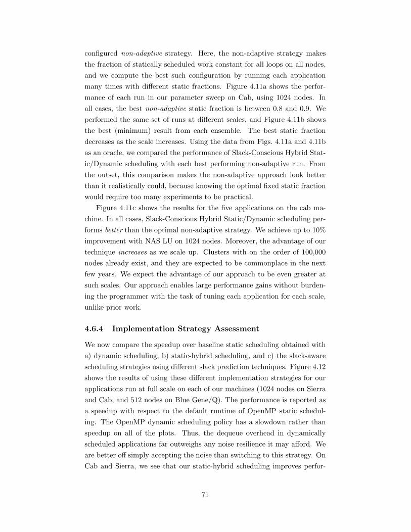
configured non-adaptive strategy. Here, the non-adaptive strategy makes
the fraction of statically scheduled work constant for all loops on all nodes,
and we compute the best such configuration by running each application
many times with different static fractions. Figure 4.11a shows the perfor-
mance of each run in our parameter sweep on Cab, using 1024 nodes. In
all cases, the best non-adaptive static fraction is between 0.8 and 0.9. We
performed the same set of runs at different scales, and Figure 4.11b shows
the best (minimum) result from each ensemble. The best static fraction
decreases as the scale increases. Using the data from Figs. 4.11a and 4.11b
as an oracle, we compared the performance of Slack-Conscious Hybrid Stat-
ic/Dynamic scheduling with each best performing non-adaptive run. From
the outset, this comparison makes the non-adaptive approach look better
than it realistically could, because knowing the optimal fixed static fraction
would require too many experiments to be practical.
Figure 4.11c shows the results for the five applications on the cab ma-
chine. In all cases, Slack-Conscious Hybrid Static/Dynamic scheduling per-
forms better than the optimal non-adaptive strategy. We achieve up to 10%
improvement with NAS LU on 1024 nodes. Moreover, the advantage of our
technique increases as we scale up. Clusters with on the order of 100,000
nodes already exist, and they are expected to be commonplace in the next
few years. We expect the advantage of our approach to be even greater at
such scales. Our approach enables large performance gains without burden-
ing the programmer with the task of tuning each application for each scale,
unlike prior work.
4.6.4 Implementation Strategy Assessment
We now compare the speedup over baseline static scheduling obtained with
a) dynamic scheduling, b) static-hybrid scheduling, and c) the slack-aware
scheduling strategies using different slack prediction techniques. Figure 4.12
shows the results of using these different implementation strategies for our
applications run at full scale on each of our machines (1024 nodes on Sierra
and Cab, and 512 nodes on Blue Gene/Q). The performance is reported as
a speedup with respect to the default runtime of OpenMP static schedul-
ing. The OpenMP dynamic scheduling policy has a slowdown rather than
speedup on all of the plots. Thus, the dequeue overhead in dynamically
scheduled applications far outweighs any noise resilience it may afford. We
are better off simply accepting the noise than switching to this strategy. On
Cab and Sierra, we see that our static-hybrid scheduling improves perfor-
71
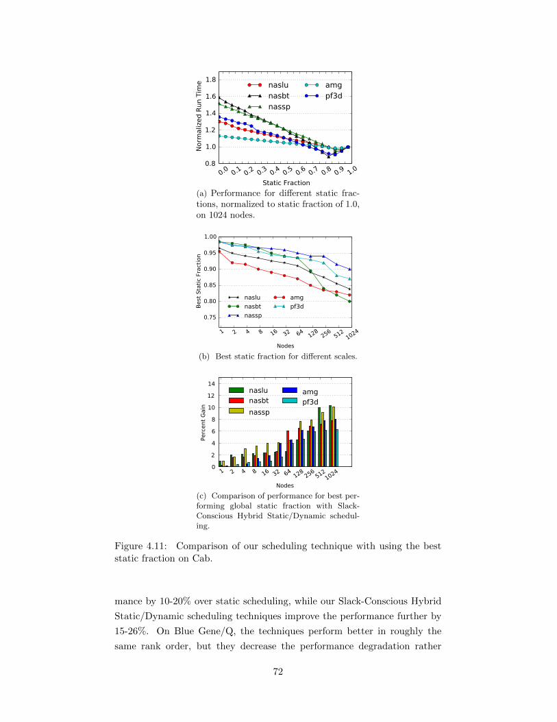
0.0 0.1 0.2 0.3 0.4 0.5 0.6 0.7 0.8 0.9 1.0
Static Fraction
0.8
1.0
1.2
1.4
1.6
1.8
Norm
aliz
ed R
un T
ime naslu
nasbtnassp
amgpf3d
(a) Performance for different static frac-tions, normalized to static fraction of 1.0,on 1024 nodes.
1 2 4 8 16 32 64128
256512
1024
Nodes
0.75
0.80
0.85
0.90
0.95
1.00
Best
Sta
tic
Fract
ion
naslu
nasbt
nassp
amg
pf3d
(b) Best static fraction for different scales.
1 2 4 8 16 32 64128
256512
1024
Nodes
0
2
4
6
8
10
12
14
Perc
ent
Gain
naslunasbt
nassp
amgpf3d
(c) Comparison of performance for best per-forming global static fraction with Slack-Conscious Hybrid Static/Dynamic schedul-ing.
Figure 4.11: Comparison of our scheduling technique with using the beststatic fraction on Cab.
mance by 10-20% over static scheduling, while our Slack-Conscious Hybrid
Static/Dynamic scheduling techniques improve the performance further by
15-26%. On Blue Gene/Q, the techniques perform better in roughly the
same rank order, but they decrease the performance degradation rather
72

nasbt nassp naslu amg pf3d
Application
60
40
20
0
20
Perc
ent
Speedup
OMP-Dynamic
Static-Hybrid
Adpt-Naive
Adpt-Collective
Adpt-Callpath
(a) Sierra.
nasbt nassp naslu amg pf3d
Application
60
40
20
0
20
Perc
ent
Speedup
OMP-Dynamic
Static-Hybrid
Adpt-Naive
Adpt-Collective
Adpt-Callpath
(b) Cab.
nasbt nassp naslu amg pf3d
Application
50
40
30
20
10
0
10
20
Perc
ent
Speedup
OMP-Dynamic
Static-Hybrid
Adpt-Naive
Adpt-Collective
Adpt-Callpath
(c) Blue Gene/Q.
Figure 4.12: Performance for different scheduling strategies shown as per-centage speedup over OpenMP static scheduling.
than getting more speedup.
Overhead Analysis
nasbt nassp naslu amg pf3dApplication
0
5
10
15
20
25
Perc
ent
of
Runti
me
OMP-Dyn
Static-Hybrid
Adpt-Naive
Adpt-Collective
Adpt-Callpath
(a) Sierra.
nasbt nassp naslu amg pf3dApplication
0
5
10
15
20
25
Perc
ent
of
Runti
me
OMP-Dyn
Static-Hybrid
Adpt-Naive
Adpt-Collective
Adpt-Callpath
(b) Cab.
nasbt nassp naslu amg pf3dApplication
0
5
10
15
20
25
Perc
ent
of
Runti
me
OMP-Dyn
Static-Hybrid
Adpt-Naive
Adpt-Collective
Adpt-Callpath
(c) Blue Gene/Q.
Figure 4.13: Overheads for different scheduling strategies as a percent oftotal runtime. Dequeue overhead is hashed, and thread idle time is solid.
To understand better how different adaptation strategies balance tran-
sient load imbalances and scheduler overhead, we measure the total time
spent across all threads in scheduler overhead and thread idle time during
execution. Figures 4.13a, 4.13b and 4.13c show the percent costs (cost is
in units of CPU-seconds) spent in thread idle time and scheduling over-
head time for Sierra, Cab and BlueGene/Q, respectively. The general trend
we see is that with the fully dynamic scheduling strategy, we incur high
percentage costs mainly due to scheduling overhead. As we use more ag-
gressively lightweight scheduling strategies (with Adpt-Callpath being most
aggressive), we increase costs of thread idle time slightly, but the cost of
scheduling overhead is greatly decreased. We also note that with Sierra,
which has lower dequeue overhead than Cab, the Adpt-Callpath strategy is
still beneficial in reducing scheduling overhead costs.
73

4.6.5 Overall Application Performance
Figures 4.14a, 4.14b, and 4.14c show the relative speedup we attain over
OpenMP static scheduling for all five applications using our Slack-Conscious
Hybrid Static/Dynamic scheduling with callpath-based slack prediction. On
1 2 4 8 16 32 64 128 256 512 1024Nodes
0
5
10
15
20
25
30
35Perc
ent
Speedup
nasbt nassp naslu amg pf3d
(a) Sierra.
1 2 4 8 16 32 64 128 256 512 1024Nodes
0
5
10
15
20
25
30
35
Perc
ent
Speedup
nasbt nassp naslu amg pf3d
(b) Cab.
1 2 4 8 16 32 64 128 256 511 512Nodes
2
1
0
1
2
3
4
5
Perc
ent
Speedup
nasbt nassp naslu amg pf3d
(c) Blue Gene/Q.
Figure 4.14: Scaling runs of all five applications.
Cab, Slack-Conscious Hybrid Static/Dynamic scheduling improves perfor-
mance in all cases. We are able to improve performance by up to 26.8% for
the NAS BT benchmark running on 1024 nodes. For real-world applications
like AMG and PF3D, we are able to achieve a 20% performance gain on
1,024 nodes. Notably, the amount of improvement increases as we scale up,
which is consistent with the idea of noise resiliency: there is more likelihood
that some node will encounter noise at scale, so the benefit of our tech-
74
niques increases. On the Blue Gene/Q machine, we see that our techniques
have much less effect. At most scales, our benchmarks and applications are
slowed down by a fraction of a percent. This is likely because we add a small
overhead to scheduling in the complete absence of noise. However, at large
scale, we are able to improve AMG performance by a few percent. AMG
has load imbalances in the sparse phases of the solve at larger scales, and
we attribute these gains to being able to compensate for these imbalances.
Because our Slack-Conscious Hybrid Static/Dynamic scheduler manages the
transient delays while also reducing dequeue overhead, we are actually able
to improve performance on a nearly “noiseless” machine, showing that our
technique can be beneficial for transient load imbalances that come from the
application and not just the platform. The key observation here is that even
on a machine with little or no noise, we do not hurt performance, and for load
imbalanced applications we can often improve it. For machines where noise
is prevalent, we achieve significant speedups with Slack-Conscious Hybrid
Static/Dynamic scheduling.
2 4 8 16 32 64 128
256
512
1024
Nodes
103
Tim
e (s
econ
ds)
OMP-StaticOMP-DynamicStatic-Hybrid
OMP-GuidedAdpt-Callpath
vSchedcomboSched
Figure 4.15: Scalability of PF3D with different schedulers on cab.
Figure 4.15 shows the raw runtimes for the PF3D application on cab. On
this system, OpenMP dynamic scheduling performs noticeably worse than
the other strategies. On Cab, both static and guided scheduling perform
roughly 10% faster than dynamic scheduling, with guided scheduling some-
times tying and sometimes coming in slightly faster. Using our static-hybrid
scheduling policy, we are able to perform faster than any built-in OpenMP
scheduling policy by approximately 9%, and using Slack-conscious schedul-
ing to exploit knowledge of the MPI runtime, we are able to run up to 18%
75
faster than stock OpenMP.
4.7 Conclusion
In this work, we have developed fundamental techniques that enable pro-
grammers to overcome the scaling wall, induced by within-node transient
delays, for hybrid parallel applications. We demonstrated a general method
that adaptively tunes itself, and which shows increasing performance im-
provement on increasingly large systems. We also implemented an auto-
mated source-to-source transformation framework for MPI+OpenMP hybrid
applications that transforms such applications in a way that is transparent
to the application programmer.
Our results showed performance gains of 26.8% over basic static schedul-
ing for NAS BT MZ running on 1,024 nodes (16,384 cores) of a NUMA clus-
ter. We showed that our Slack-Conscious Hybrid Static/Dynamic scheduler
will not hurt performance significantly on a low-noise machine, and may im-
prove the performance of load imbalanced applications even when there is
no noise. Most importantly, we showed that our performance gains increase
for increasingly large scales, indicating that our approach will yield even
more improvement on future systems.
76
Chapter 5
Spatial Locality inDynamically AssignedIterationsThe hybrid static/dynamic scheduling scheme provides many performance
benefits. In particular, the statically allocated iterations exhibit higher spa-
tial and temporal locality. In consecutive outer iterations, each thread exe-
cutes the same inner loop iterations and therefore touches the same data on
each outer iteration. In addition, statically allocated iterations for a given
thread constitute a contiguous region, and thus exhibit spatial locality (this
assumes consecutive iterations access nearby data, which is the common case
in most applications). However, for dynamically allocated iterations, spatial
as well as outer-loop temporal locality is lost. In this chapter, we develop a
technique to restore locality for these iterations.
To handle a larger class of load imbalances so as to make our approach
useful to a broad range of applications, we consider modifications to our
existing hybrid static/dynamic scheduling scheme to improve data locality.
Specifically, we implement a scheduling scheme in which we change the lay-
out of the iterations that are static and the iterations that are dynamic, in
order to improve spatial locality. We also add an additional tunable con-
straint in the dequeue function of the scheduler, in order to reduce coherence
cache misses on a multi-core node. The constraint is quantified as a fraction
of dynamically scheduled work, and thus can be determined through perfor-
mance modeling and theoretical analysis in the same way as done in [27].
The contributions of this chapter are:
1. Analysis of the tradeoff between locality and load balance for coarse-
grained application-generated imbalances;
2. Improvement of spatial locality for scheduling in current static/dy-
namic scheduling schemes;
3. Techniques (constraints) for the portion of work that is dynamically
scheduled, so as to reduce both coherence cache misses and contention
on the shared memory interconnect.
77
Through experimentation of an N-body code on modern multi-core ar-
chitectures, our technique gives 19.42% performance gains over dynamic
scheduling, and an overall 48.63% gain over standard static scheduling.
5.1 Problem Statement
The scheduling strategy in this chapter builds upon the basic hybrid stat-
ic/dynamic scheduling strategy of Chapter 2. So, we begin with a recap
of that strategy. We assume a bulk-synchronous hybrid MPI+OpenMP or
MPI+pthread application, where each thread runs on one core of an SMP
node (and each MPI process runs on one node). A bulk-synchronous code
consists of several application timesteps, with each application timestep sur-
rounded by two successive global MPI collective invocations. Within each
timestep are one or more threaded computation regions, e.g., a loop per-
forming a dot product with a #pragma omp parallel for surrounded
by it. Unless otherwise noted, a threaded computation region ends with a
thread barrier. There may be load imbalance across threads, not just of the
magnitude of one loop iteration, i.e., fine-grained, but also of the magnitude
of multiple loop iterations, i.e., coarse-grained. This load imbalance may
come from either system noise or from the application. The characteristic
of load imbalance may be transient, i.e., without a fixed pattern across ap-
plication timesteps, or persistent, i.e., with a fixed pattern across application
timesteps.
A simple technique to handle the load imbalance within a node during
the execution of an application timestep is to use dynamic scheduling rather
than standard static scheduling. We assume a dynamic scheduling strategy
where, during each invocation of a threaded computation region, threads
pull sets of loop iterations, or tasklets, from a shared work queue. These
tasklets have locality tags associated with them that indicate the thread
on which that tasklet ran in the last application timestep. The scheduler
attempts to give a thread a tasklet that the thread executed in the previous
outer iteration, to the extent possible. Let us assume that when a thread
retrieves a tasklet from the shared work queue, it incurs some scheduler
overhead, consisting of dequeue overhead due to locking (including waiting
for the lock) and unlocking the queue to retrieve a tasklet, along with the
possible cost of data movement overhead due to coherence cache misses
required to retrieve data corresponding to iterations specified by the tasklet
from another core.
To reduce these costs of dynamic load balancing, a hybrid static/dy-
78
namic scheduling scheme can be used. In this scheme, depicted in Figure 5.1,
threads first execute pre-assigned iterations from a fraction of iterations of
the compute loop.The threads then, without waiting at a thread barrier, ex-
ecute the remaining fraction of iterations dynamically by retrieving tasklets
from a shared work queue. The x-axis in the figure is iterations, and not
time. The point in the computation at which the threads switch from static
scheduling to dynamic scheduling is either empirically tuned or determined
through performance modeling and theoretical analysis.
5.2 Scheduling Strategy
We explain the locality optimizations of the hybrid static/dynamic schedul-
ing strategies that we use to improve performance. In the following, let p be
the number of cores on an SMP node. Let n be the number of iterations in
a loop. Let fs be the fraction of statically scheduled iterations of the loop.
Let t be the thread ID of a particular thread participating in a threaded
computation region.
5.2.1 Modifications to Allocation of Iterations
A key problem of spatial locality exists with hybrid static/dynamic schedul-
ing. Figure 5.1 shows the allocation of iterations to threads. In the diagram,
the x-axis is loop iteration number. Consider the dynamically scheduled set
of loop iterations, starting with the iteration numbered n·fsp , in Figure 5.1.
As the labeling indicates, iterations are executed by arbitrary threads de-
pending on the order in which the threads requested work.
Across outer iterations, the same inner iteration will typically be exe-
cuted by different threads, and therefore will access data that was used by
a different thread earlier. Heuristically, we can assume that consecutive it-
erations access adjacent data. This is because programmers typically write
code to preserve spatial locality. Note that in the dynamic section, this
spatial locality is also lost, where the consecutive sets of loop iterations get
allocated to different threads arbitrarily.
Can we control the arbitrariness of the allocation of dynamic iterations
to reduce the above problem? Consider the case of transient noise. We note
that on a given node, on most outer iterations, there will be no noise. Yet,
the dynamic scheduler will necessarily be arbitrary given the order in which
the threads will enter the critical section to fetch their dynamic allocations.
We prefer that the dynamic iterations executed by a thread be contiguous
to its static allocation, to the extent possible.
79

dynamicstatic
Increasing loop iteration number
T0 T1 T2 T3 T3T2T2T0T1T1T2T0..
Figure 5.1: Allocation of iterations to threads for Hybrid Static/DynamicScheduling.
Therefore, we rearrange the static and dynamic iterations so that for
each thread, the dynamic iterations are placed after the static iterations.
That is, when a thread completes its last statically scheduled iteration i,
the first dynamically allocated iteration it receives is likely to be i+ 1. This
new layout is shown in Figure 5.2. Now, thread t begins its static section atn·tp , and ends it before n·(t+fs)
p . Most importantly, each thread t maintains
a separate queue of tasklets that corresponds to iterations contiguous to its
static iterations, namely from n·(t+fs)p to n·(t+1)
p .
Each thread first executes its static iterations, and then dynamically
allocates iterations from its own dynamic queue. Only after that does it
attempt to steal work from other queues. When there is no imbalance, each
thread will execute a contiguous set of iterations (static + dynamic) just
as an OpenMP static scheduler will. Even when a core is overloaded by
noise, the rest of the cores execute their own dynamic iterations first before
helping the overloaded cores. Therefore, most dynamic iterations retain
outer iteration locality as well as spatial locality.
static dyn
Increasing loop iteration number
dyn dyn dynstatic static static
T0 T1 T2 T3T0 T1 T2 T3
Figure 5.2: Allocation of loop iterations to threads for Staggered HybridStatic/Dynamic Scheduling.
5.2.2 Choosing the Thread From Which to Steal
A basic problem with the dynamic scheduling section of hybrid static/dy-
namic scheduling is that it incurs overhead due to scheduling from a shared
queue, as is done in many dynamic scheduling implementations. This causes
additional locking and synchronization overhead, especially as the number
80
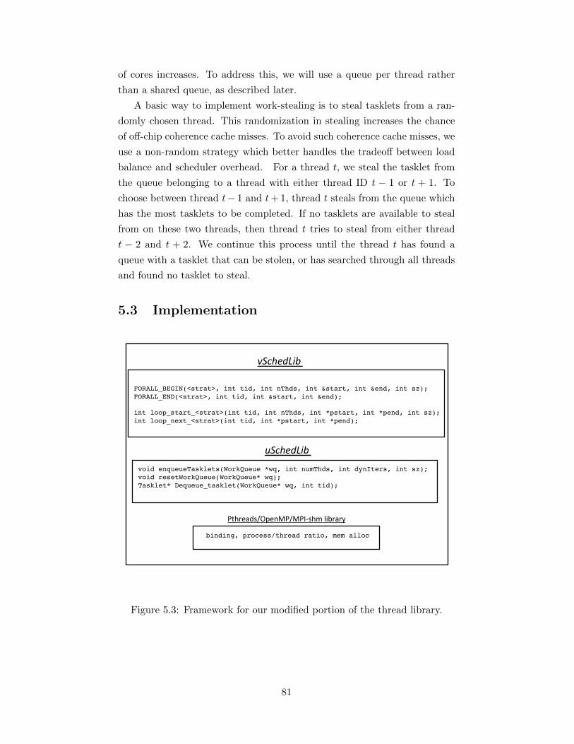
of cores increases. To address this, we will use a queue per thread rather
than a shared queue, as described later.
A basic way to implement work-stealing is to steal tasklets from a ran-
domly chosen thread. This randomization in stealing increases the chance
of off-chip coherence cache misses. To avoid such coherence cache misses, we
use a non-random strategy which better handles the tradeoff between load
balance and scheduler overhead. For a thread t, we steal the tasklet from
the queue belonging to a thread with either thread ID t − 1 or t + 1. To
choose between thread t− 1 and t+ 1, thread t steals from the queue which
has the most tasklets to be completed. If no tasklets are available to steal
from on these two threads, then thread t tries to steal from either thread
t − 2 and t + 2. We continue this process until the thread t has found a
queue with a tasklet that can be stolen, or has searched through all threads
and found no tasklet to steal.
5.3 Implementation
FORALL_BEGIN(<strat>, int tid, int nThds, int &start, int &end, int sz);!FORALL_END(<strat>, int tid, int &start, int &end);!
int loop_start_<strat>(int tid, int nThds, int *pstart, int *pend, int sz);!int loop_next_<strat>(int tid, int *pstart, int *pend);!
binding, process/thread ratio, mem alloc!
vSchedLib
uSchedLib
Pthreads/OpenMP/MPI-‐shm library
void enqueueTasklets(WorkQueue *wq, int numThds, int dynIters, int sz); !void resetWorkQueue(WorkQueue* wq);!Tasklet* Dequeue_tasklet(WorkQueue* wq, int tid);!
Figure 5.3: Framework for our modified portion of the thread library.
81
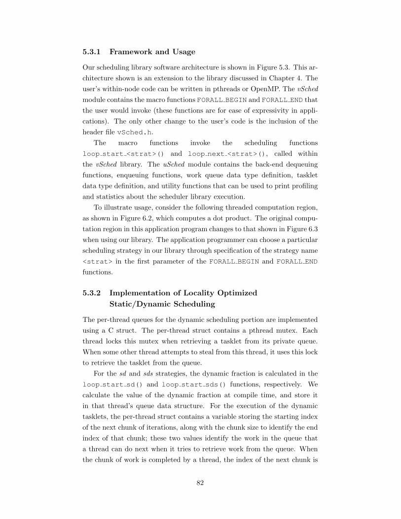
5.3.1 Framework and Usage
Our scheduling library software architecture is shown in Figure 5.3. This ar-
chitecture shown is an extension to the library discussed in Chapter 4. The
user’s within-node code can be written in pthreads or OpenMP. The vSched
module contains the macro functions FORALL BEGIN and FORALL END that
the user would invoke (these functions are for ease of expressivity in appli-
cations). The only other change to the user’s code is the inclusion of the
header file vSched.h.
The macro functions invoke the scheduling functions
loop start <strat>() and loop next <strat>(), called within
the vSched library. The uSched module contains the back-end dequeuing
functions, enqueuing functions, work queue data type definition, tasklet
data type definition, and utility functions that can be used to print profiling
and statistics about the scheduler library execution.
To illustrate usage, consider the following threaded computation region,
as shown in Figure 6.2, which computes a dot product. The original compu-
tation region in this application program changes to that shown in Figure 6.3
when using our library. The application programmer can choose a particular
scheduling strategy in our library through specification of the strategy name
<strat> in the first parameter of the FORALL BEGIN and FORALL END
functions.
5.3.2 Implementation of Locality Optimized
Static/Dynamic Scheduling
The per-thread queues for the dynamic scheduling portion are implemented
using a C struct. The per-thread struct contains a pthread mutex. Each
thread locks this mutex when retrieving a tasklet from its private queue.
When some other thread attempts to steal from this thread, it uses this lock
to retrieve the tasklet from the queue.
For the sd and sds strategies, the dynamic fraction is calculated in the
loop start sd() and loop start sds() functions, respectively. We
calculate the value of the dynamic fraction at compile time, and store it
in that thread’s queue data structure. For the execution of the dynamic
tasklets, the per-thread struct contains a variable storing the starting index
of the next chunk of iterations, along with the chunk size to identify the end
index of that chunk; these two values identify the work in the queue that
a thread can do next when it tries to retrieve work from the queue. When
the chunk of work is completed by a thread, the index of the next chunk is
82
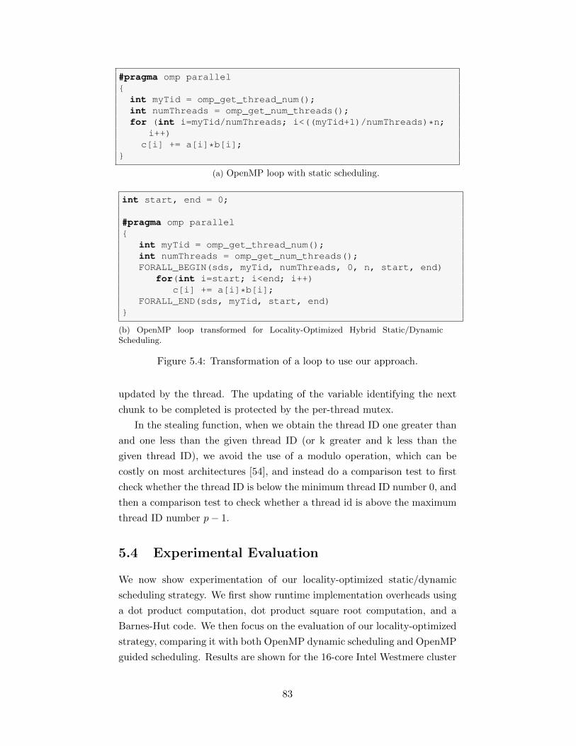
#pragma omp parallel{
int myTid = omp_get_thread_num();int numThreads = omp_get_num_threads();for (int i=myTid/numThreads; i<((myTid+1)/numThreads)*n;
i++)c[i] += a[i]*b[i];
}
(a) OpenMP loop with static scheduling.
int start, end = 0;
#pragma omp parallel{
int myTid = omp_get_thread_num();int numThreads = omp_get_num_threads();FORALL_BEGIN(sds, myTid, numThreads, 0, n, start, end)
for(int i=start; i<end; i++)c[i] += a[i]*b[i];
FORALL_END(sds, myTid, start, end)}
(b) OpenMP loop transformed for Locality-Optimized Hybrid Static/DynamicScheduling.
Figure 5.4: Transformation of a loop to use our approach.
updated by the thread. The updating of the variable identifying the next
chunk to be completed is protected by the per-thread mutex.
In the stealing function, when we obtain the thread ID one greater than
and one less than the given thread ID (or k greater and k less than the
given thread ID), we avoid the use of a modulo operation, which can be
costly on most architectures [54], and instead do a comparison test to first
check whether the thread ID is below the minimum thread ID number 0, and
then a comparison test to check whether a thread id is above the maximum
thread ID number p− 1.
5.4 Experimental Evaluation
We now show experimentation of our locality-optimized static/dynamic
scheduling strategy. We first show runtime implementation overheads using
a dot product computation, dot product square root computation, and a
Barnes-Hut code. We then focus on the evaluation of our locality-optimized
strategy, comparing it with both OpenMP dynamic scheduling and OpenMP
guided scheduling. Results are shown for the 16-core Intel Westmere cluster
83

Code Pct. ovhd
dotProd 3.14%
dotProdSqrt 2.31%
Barnes-Hut 1.71%
Regular Mesh 2.12%
Table 5.1: Overheads of our scheduling runtime shown as the percentage dif-ference between our library’s static scheduling and OpenMP static schedul-ing.
with a CHAOS 4.4 Linux-based operating system.
For the Barnes-Hut code, we show in Figure 5.5 the main modification
done. Specifically, the modified code is shown within the #ifdef CDY
... #else portion of the code. The original pthreads code is shown in the
#else... #endif portion of the code. The start and end variables, which
are private to each thread, are calculated from within our scheduler library.
5.4.1 Implementation Overhead
Table 5.1 shows the comparison between our library’s static scheduling and
OpenMP static scheduling for three different codes. The first code is a dot
product calculation, denoted dotProd. To increase the computation per
step of this dot product code, we applied a square root function to each
product, denoted dotProdSqrt. We also show the result for the Barnes-
Hut code, denoted by its name below. The comparison between our library
implementation and the OpenMP library implementation is done by taking
the percentage loss in execution time of our static scheduling method (100%
static) with respect to OpenMP static scheduling.
The overheads in our implementation are small even for the code with
very little work in each timestep (1000 timesteps were done), i.e., for the
dot product computation, and decreases slightly when we increase the com-
putation done, specifically for the square rooted dot product computation.
We also see that the overheads are notably low for Barnes-Hut code, where
the computation per step is significantly larger than both the dotProd and
dotProdSqrt. From this, we can justify that our library is adequately op-
timized. Further optimizations can be done to reduce other overheads of
library operation, but these small overheads do not add significant perfor-
mance degradation to application execution when using our runtime.
84
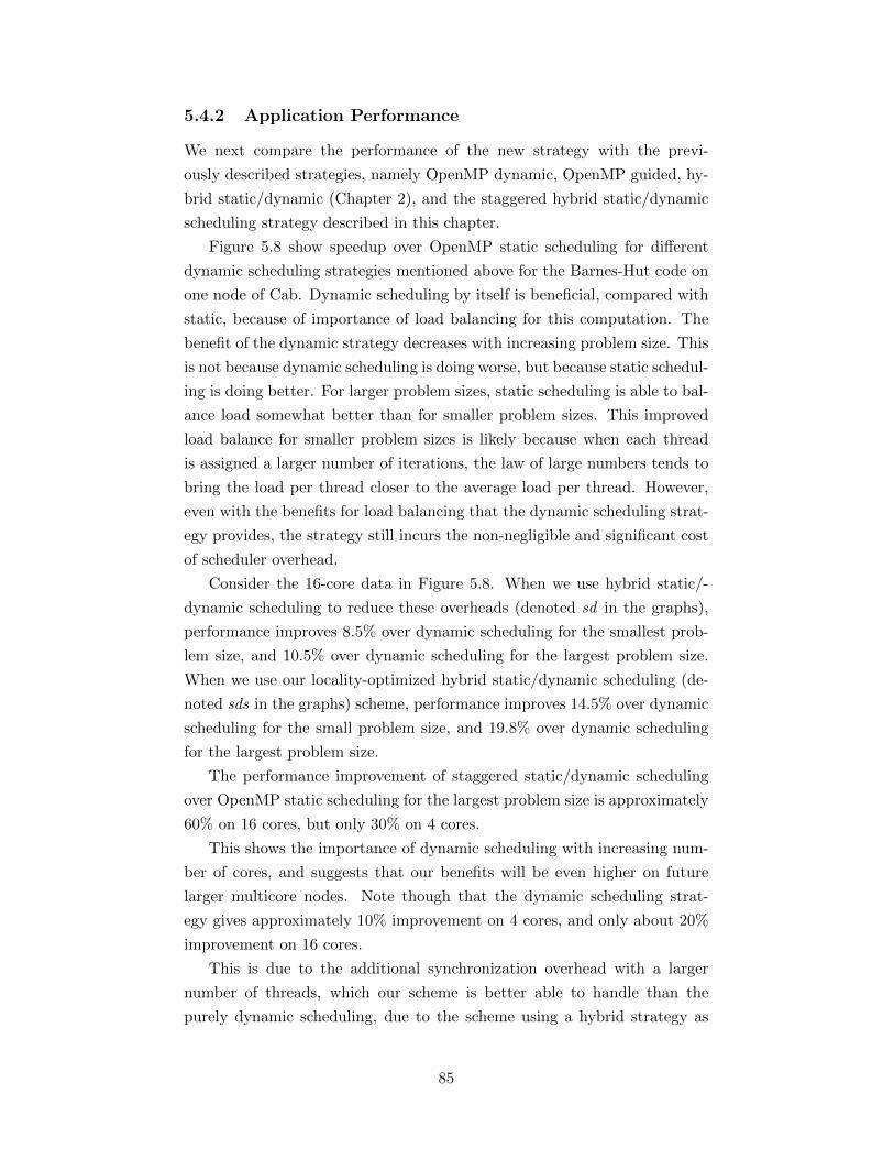
5.4.2 Application Performance
We next compare the performance of the new strategy with the previ-
ously described strategies, namely OpenMP dynamic, OpenMP guided, hy-
brid static/dynamic (Chapter 2), and the staggered hybrid static/dynamic
scheduling strategy described in this chapter.
Figure 5.8 show speedup over OpenMP static scheduling for different
dynamic scheduling strategies mentioned above for the Barnes-Hut code on
one node of Cab. Dynamic scheduling by itself is beneficial, compared with
static, because of importance of load balancing for this computation. The
benefit of the dynamic strategy decreases with increasing problem size. This
is not because dynamic scheduling is doing worse, but because static schedul-
ing is doing better. For larger problem sizes, static scheduling is able to bal-
ance load somewhat better than for smaller problem sizes. This improved
load balance for smaller problem sizes is likely because when each thread
is assigned a larger number of iterations, the law of large numbers tends to
bring the load per thread closer to the average load per thread. However,
even with the benefits for load balancing that the dynamic scheduling strat-
egy provides, the strategy still incurs the non-negligible and significant cost
of scheduler overhead.
Consider the 16-core data in Figure 5.8. When we use hybrid static/-
dynamic scheduling to reduce these overheads (denoted sd in the graphs),
performance improves 8.5% over dynamic scheduling for the smallest prob-
lem size, and 10.5% over dynamic scheduling for the largest problem size.
When we use our locality-optimized hybrid static/dynamic scheduling (de-
noted sds in the graphs) scheme, performance improves 14.5% over dynamic
scheduling for the small problem size, and 19.8% over dynamic scheduling
for the largest problem size.
The performance improvement of staggered static/dynamic scheduling
over OpenMP static scheduling for the largest problem size is approximately
60% on 16 cores, but only 30% on 4 cores.
This shows the importance of dynamic scheduling with increasing num-
ber of cores, and suggests that our benefits will be even higher on future
larger multicore nodes. Note though that the dynamic scheduling strat-
egy gives approximately 10% improvement on 4 cores, and only about 20%
improvement on 16 cores.
This is due to the additional synchronization overhead with a larger
number of threads, which our scheme is better able to handle than the
purely dynamic scheduling, due to the scheme using a hybrid strategy as
85

well as its use of localized work queues.
Comparing with Guided Scheduling: Our strategy improves per-
formance 10.1% over OpenMP guided scheduling for the smallest problem
size, and 14.3% for the largest problem size. Guided scheduling incurs addi-
tional data movement because it does not respect outer iteration locality as
well as spatial locality, whereas our scheduling scheme limits this dequeue
overhead through the use of partially static scheduling.
Table 5.2 shows the standard deviations of execution times across 15
trials of the Barnes-Hut code, where a trial is a single job submission of
the code. The dynamic and guided scheduling schemes exhibit over 6.2%
standard deviation, and the sd strategy improves the standard deviation to
4.1%. Our sds scheduling further reduces the standard deviation to 1.9%.
This is likely due to its superior outer iteration locality in both static and
dynamic sections of iterations. This low standard deviation shows perfor-
mance consistency, which is beneficial for bulk-synchronous codes, as shown
in [27,54].
static void* Process(void* arg){
register const int slice = (long) arg;int start, end;
#ifdef CDY_ // constrained dynamic schedulingint tid = (long) arg;int i;setCDY(fd, myConstraint, chunkSz);FORALL_BEGIN(sds, 0, nbodies, start, end, tid, thds)
for (i=start; i<end; i++)body[i]->ComputeForce(groot, gdiameter);
FORALL_END(sds, start, end, myTid)#else // normal pthreads code
start = slice * nbodies / threads;end = (slice + 1) * nbodies / threads;// the iterations can be executed in any orderfor (int i = start; i < end; i++) {
// compute the acceleration of each body//(consumes most of the runtime)body[i]->ComputeForce(groot, gdiameter);
}#endif
return NULL;}
Figure 5.5: Barnes-Hut code main modification using Slack-Conscious Hy-brid Static/Dynamic scheduling.
86

We briefly explain the impact of the sds strategy on load balanced com-
putations. Recall that we consider dynamic strategies for such computations
is because of transient imbalances, a.k.a. noise. We have explained and
experimented with the relationship between single-node performance and
multi-node performance going to a large number of nodes, in the presence
of noise. We therefore focus on single-node performance in this chapter.
Specifically, for load balanced computations, our objective is to show that
our schemes do not add significant overhead to static scheduling. This can
help to ensure that on large number of nodes, the dynamic component of
our schemes will control the amplification as described in Chapter 2. In
this context, we show the performance of multiple scheduling strategies on
the stencil computation of Chapter 2 in Figure 5.9. The sds strategy does
slightly, but consistently better than the sd strategy because of the im-
proved locality in the dynamic section. The guided scheduling strategy does
slightly better on the two smallest problem sizes, but much worse on the
largest problem size, compared with sds. This again shows the consistency
benefit of sds. We believe that the benefit of guided can be overcome by
increasing the chunk size in sds.
1000 10000 100000Number of Bodies
0.0
0.1
0.2
0.3
0.4
0.5
0.6
0.7
Impro
vem
ent
OMP-Dynamic OMP-Guided uSched vSched
Figure 5.6: Improvement obtained over OpenMP static scheduling for dif-ferent scheduling strategies applied to Barnes-Hut, shown for 4 of 16 coresof Cab.
5.5 Conclusion
In this work, we showed different techniques to increase locality further
and to reduce costs of scheduling in the hybrid static/dynamic scheduling
technique, which allows for reducing performance degradation at scale for
87
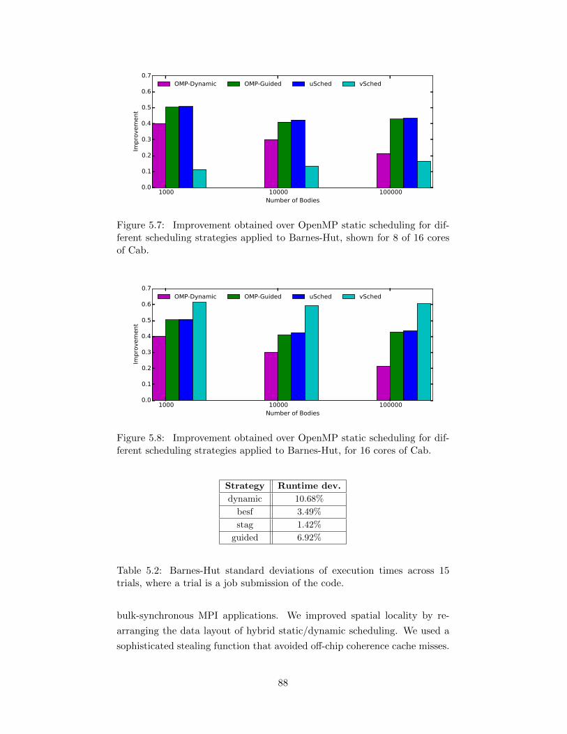
1000 10000 100000Number of Bodies
0.0
0.1
0.2
0.3
0.4
0.5
0.6
0.7
Impro
vem
ent
OMP-Dynamic OMP-Guided uSched vSched
Figure 5.7: Improvement obtained over OpenMP static scheduling for dif-ferent scheduling strategies applied to Barnes-Hut, shown for 8 of 16 coresof Cab.
1000 10000 100000Number of Bodies
0.0
0.1
0.2
0.3
0.4
0.5
0.6
0.7
Impro
vem
ent
OMP-Dynamic OMP-Guided uSched vSched
Figure 5.8: Improvement obtained over OpenMP static scheduling for dif-ferent scheduling strategies applied to Barnes-Hut, for 16 cores of Cab.
Strategy Runtime dev.
dynamic 10.68%
besf 3.49%
stag 1.42%
guided 6.92%
Table 5.2: Barnes-Hut standard deviations of execution times across 15trials, where a trial is a job submission of the code.
bulk-synchronous MPI applications. We improved spatial locality by re-
arranging the data layout of hybrid static/dynamic scheduling. We used a
sophisticated stealing function that avoided off-chip coherence cache misses.
88
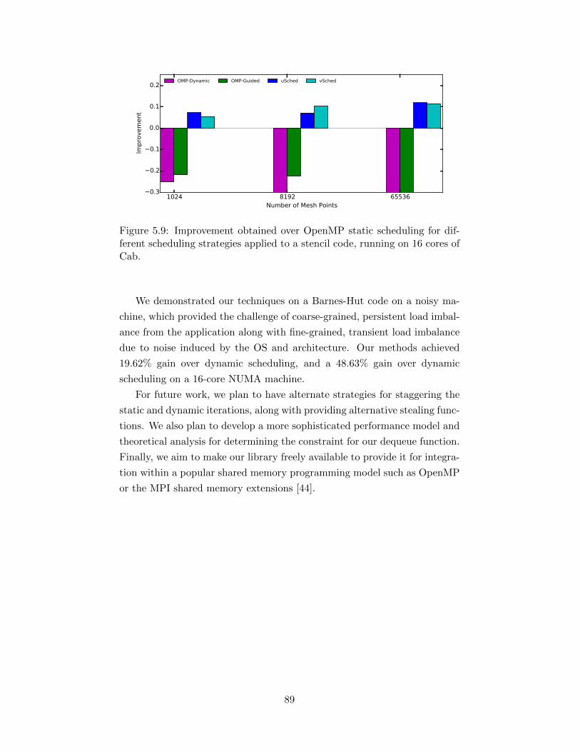
1024 8192 65536Number of Mesh Points
0.3
0.2
0.1
0.0
0.1
0.2
Impro
vem
ent
OMP-Dynamic OMP-Guided uSched vSched
Figure 5.9: Improvement obtained over OpenMP static scheduling for dif-ferent scheduling strategies applied to a stencil code, running on 16 cores ofCab.
We demonstrated our techniques on a Barnes-Hut code on a noisy ma-
chine, which provided the challenge of coarse-grained, persistent load imbal-
ance from the application along with fine-grained, transient load imbalance
due to noise induced by the OS and architecture. Our methods achieved
19.62% gain over dynamic scheduling, and a 48.63% gain over dynamic
scheduling on a 16-core NUMA machine.
For future work, we plan to have alternate strategies for staggering the
static and dynamic iterations, along with providing alternative stealing func-
tions. We also plan to develop a more sophisticated performance model and
theoretical analysis for determining the constraint for our dequeue function.
Finally, we aim to make our library freely available to provide it for integra-
tion within a popular shared memory programming model such as OpenMP
or the MPI shared memory extensions [44].
89
Chapter 6
Composing MultipleScheduling Strategies
In the previous chapters, we discussed the reasons for using basic hybrid
static/dynamic scheduling techniques, and discussed additional optimiza-
tions over hybrid static/dynamic scheduling. However, for real applications
running on real-world architectures, several different factors of the machine
and application are involved. Thus, we need to find a way to handle all
of the problems discussed, simultaneously. In this chapter, we discuss a
methodology to combine the scheduling schemes to make it available for the
user.
To do this, we first identify the general types of scheduler techniques we
have discussed up to this point, and combine them to make them usable for
the application programmer within software. We discuss implementation a
scheduler composition containing all the different schedulers implemented
up to this point. With this, we show results for 3 new application codes on
different architectures, shown for different types of scheduling strategies dis-
cussed up to this point. We include notes and data on architecture-specific
tuning for the scheduler and application programmer usability. Finally, we
conclude the chapter through discussion of scheduling techniques and the
composed scheduler described in this chapter as it could be used for in the
context of running applications on next-generation architectures.
6.1 Scheduling Strategies Overview
We have examined several schedulers in the previous chapters. In different
circumstances, features of different schedulers will be more useful. It is desir-
able to combine features of different schedulers to make more sophisticated
schedulers with better performance.
To do this, we first describe categories of circumstances, features of
schedulers, methods of tuning their parameters, and performance factors.
1. circumstances: these are the architecture and application characteris-
tics that affect the choice of the scheduling strategies.
90
2. scheduler features: these are the individual techniques that were used
in putting together the schedulers of previous chapters. Our attempt
will be to judiciously choose and combine features from individual
schedulers.
3. methods for selecting parameters.
4. performance facets: the different features impact the performance via
affecting specific performance facets.
Circumstances: The application-platform combinations that we encounter
can be classified based on the following circumstances:
• noise
• application imbalance
• different iterations take different amounts of time
• effective core speed variation
• number of nodes
• number of cores per node
Features: Each of the schedulers from the previous chapters was built using
a combination of scheduling techniques. Each scheduling technique can be
thought of as a separate feature that can often be independently combined.
• hybrid static/dynamic scheduling
• chunking of iterations,(task quantization)
• variable-sized tasklets, as in guided and tasklet library.
• separate calculation of fd for each node.(forgetting about slack)
• exploiting slack
• weighted scheduling
• staggered
Methods for selecting parameters: Many of the features described
above can be refined further by selection of parameters. Also, when we
combine features from different schedulers, needs for balancing the tradeoffs
involved can be satisfied by creating additional parameters that can be ad-
justed. For example, the tradeoff between idle time and grain size, or the
tradeoff between idle time and locality.
91
• model-driven determination
• experimental tuning
• runtime adjustment
Performance facets: Different scheduling strategies impact overall appli-
cation performance in multiple ways. Although execution time is the most
important metric, several intermediate metrics provide useful insights. Spe-
cific scheduling strategies may worsen one metric while improving another.
Understanding these tradeoffs is critical to design combined schedulers that
serve any specific purpose such as the needs of an application class of in-
terest. We describe below the most important performance facets, i.e., the
intermediate metrics.
• idle time
• synchronization
• spatial locality (in dynamic section)
• spatial locality (static section)
• temporal locality (across outer iterations)
6.2 Techniques for Composing Schedulers
To illustrate how to combine schedulers, we show a particular sequence of
composition of a subset of the schedulers from previous chapters. In the
process, we will generate a new scheduler, which we call comboSched, that
combines several features from each of the baseline schedulers. The sequence
of development of these schedulers is shown in Figure 6.1.
We first review the definition of the basic lightweight scheduling tech-
nique, as it is described in previous chapters. With this defined, we explain
each of three schedulers, each based on a scheduler we have described in
the previous chapter. In some cases, these are improved versions of the
corresponding schedulers. We give a description of each scheduler, and its
specific features, especially from the point of view of how to combine them
with each other.
92
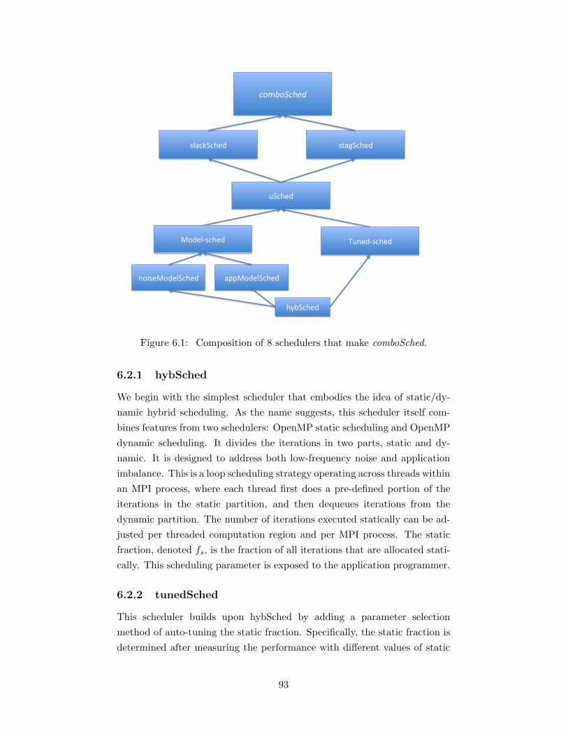
uSched
slackSched stagSched
comboSched
Model-‐sched Tuned-‐sched
hybSched
noiseModelSched appModelSched
Figure 6.1: Composition of 8 schedulers that make comboSched.
6.2.1 hybSched
We begin with the simplest scheduler that embodies the idea of static/dy-
namic hybrid scheduling. As the name suggests, this scheduler itself com-
bines features from two schedulers: OpenMP static scheduling and OpenMP
dynamic scheduling. It divides the iterations in two parts, static and dy-
namic. It is designed to address both low-frequency noise and application
imbalance. This is a loop scheduling strategy operating across threads within
an MPI process, where each thread first does a pre-defined portion of the
iterations in the static partition, and then dequeues iterations from the
dynamic partition. The number of iterations executed statically can be ad-
justed per threaded computation region and per MPI process. The static
fraction, denoted fs, is the fraction of all iterations that are allocated stati-
cally. This scheduling parameter is exposed to the application programmer.
6.2.2 tunedSched
This scheduler builds upon hybSched by adding a parameter selection
method of auto-tuning the static fraction. Specifically, the static fraction is
determined after measuring the performance with different values of static
93

fractions.
6.2.3 NoiseModelSched
Builds upon the hybSched by using a model for execution time given param-
eters of the duration of noise δnoise. See Chapter 4 for how the static fraction
is calculated using this model. For each node used for the application run,
we obtain the noise event length, tnoise, and time for dequeue operation,
tq. Note that tq and tnoise is obtained before the application begins. We
obtain the overhead due to noise and overhead due to dequeue operations
as described in Section 5.3 of Chapter 4. In Chapter 2 and Chapter 4, we
referred to the value of the noise event length as δ, but here, we will call
it δnoise so that we can distinguish load imbalance due to noise and load
imbalance due to any other source.
6.2.4 AppModelSched
Builds upon the hybSched by developing a model for execution time in
presence of application imbalance. This involves replacing the δnoise by a
measure of within-node application imbalance, δapp.
To obtain δapp, we first run 1 step of the application twice: one using
static scheduling and the other using dynamic scheduling. Specifically, we
run the application code with OpenMP static scheduling on process 0, and
then run the application code with OpenMP dynamic scheduling on process
0. For each process, we calculate the average idle time across threads within
the process from the previous application timestep. The scheduling over-
head, tovhd, is computed by multiplying the iterations per thread d by the
time for a dequeue operation tq, where tq is obtained from the measurements
of dynamic scheduling as above.
Let the time for the statically scheduled run be tstatic, the time for the
dynamically scheduled run be tdynamic, and the time for scheduler overhead
be tovhd. The magnitude of the additional duration induced by load im-
balance coming from the application, δapp, is tstatic - tdynamic - tovhd1. We
estimate the parallel outer iteration time as Tp by running the application
in a mode where only one core of each node is used, i.e., we remove the
OpenMP parallelism. We obtain the execution time on node 0, as a sample,
and divide it by the total number of cores used for the run. Instead of using
node 0 as a sample, we could use an average across all the nodes, by doing
1Alternatively, δapp can be calculated via the method used in Figure 1.2.
94
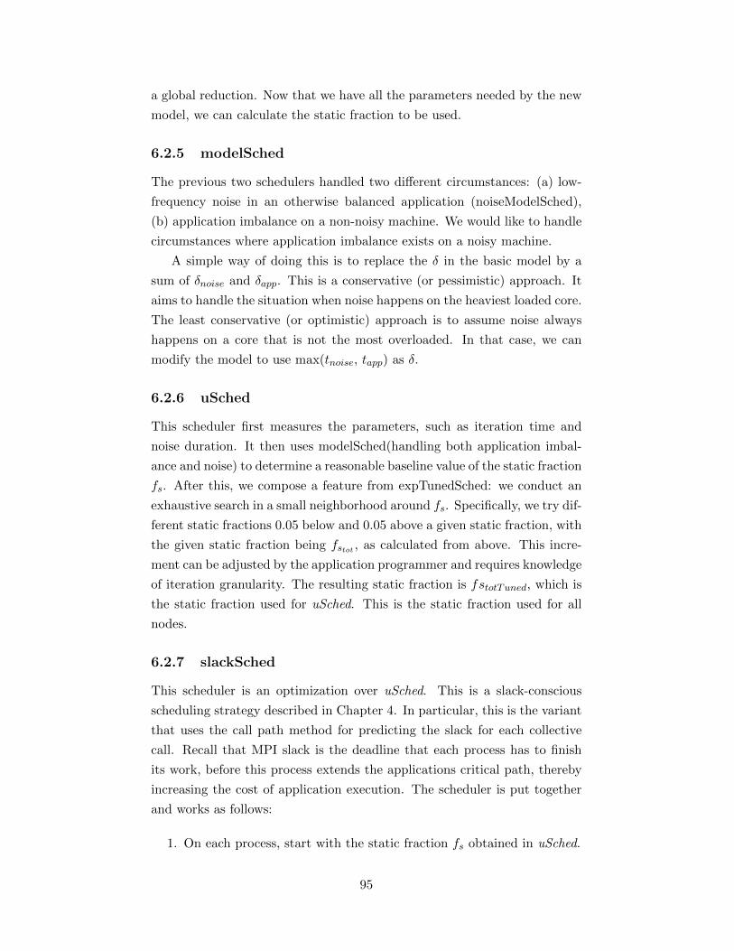
a global reduction. Now that we have all the parameters needed by the new
model, we can calculate the static fraction to be used.
6.2.5 modelSched
The previous two schedulers handled two different circumstances: (a) low-
frequency noise in an otherwise balanced application (noiseModelSched),
(b) application imbalance on a non-noisy machine. We would like to handle
circumstances where application imbalance exists on a noisy machine.
A simple way of doing this is to replace the δ in the basic model by a
sum of δnoise and δapp. This is a conservative (or pessimistic) approach. It
aims to handle the situation when noise happens on the heaviest loaded core.
The least conservative (or optimistic) approach is to assume noise always
happens on a core that is not the most overloaded. In that case, we can
modify the model to use max(tnoise, tapp) as δ.
6.2.6 uSched
This scheduler first measures the parameters, such as iteration time and
noise duration. It then uses modelSched(handling both application imbal-
ance and noise) to determine a reasonable baseline value of the static fraction
fs. After this, we compose a feature from expTunedSched: we conduct an
exhaustive search in a small neighborhood around fs. Specifically, we try dif-
ferent static fractions 0.05 below and 0.05 above a given static fraction, with
the given static fraction being fstot , as calculated from above. This incre-
ment can be adjusted by the application programmer and requires knowledge
of iteration granularity. The resulting static fraction is fstotTuned, which is
the static fraction used for uSched. This is the static fraction used for all
nodes.
6.2.7 slackSched
This scheduler is an optimization over uSched. This is a slack-conscious
scheduling strategy described in Chapter 4. In particular, this is the variant
that uses the call path method for predicting the slack for each collective
call. Recall that MPI slack is the deadline that each process has to finish
its work, before this process extends the applications critical path, thereby
increasing the cost of application execution. The scheduler is put together
and works as follows:
1. On each process, start with the static fraction fs obtained in uSched.
95

(a) On each process, retrieve that process’s invocation of the last
MPI collective, where the invocation of the last MPI collective is
retrieved through the callsite slack-prediction method (see paper
for details on implementation details of slack prediction).
(b) Given the identifier of the last the MPI collective call invoked,
estimate that collective call’s slack value from the history of slack
values stored by the slack-conscious runtime. The slack estimate
is based on the slack value recorded in the previous MPI collective
invocation, as is done in the cited work of Adagio.
2. On each process, adjust its dynamic fraction based on the slack value.
This adjustment is done using the formula 5 in section 3 of Chapter 4
(final formula defining the slack-conscious dynamic) and implementa-
tion of section 4 of Chapter 4. The static fraction used in the loop
bound is 1- fd.
Note that the dynamic fraction, rather than the static fraction (used in
Chapters 2, 3, and 5) was used in Chapter 4 to make the slack-conscious
scheduling technique more intuitive. Additionally, doing the theoretical
analysis in that chapter using the dynamic fraction rather than the static
fraction helped more to minimize the calculations needed for slack-conscious
runtime adjustment of the hybrid static/dynamic scheduling during execu-
tion of an MPI application.
6.2.8 vSched
This scheduler is based on Chapter 5. The motivation of this scheduler is
to improve the spatial locality in the dynamically scheduled iterations. In
uSched, the dynamically scheduled iterations are assigned to threads arbi-
trarily based on the order in which threads happen to request dynamic work
(see Figure 5.2). The focus of this scheduler is to use different dimensions of
the tradeoff between load balance and locality to improve upon basic hybrid
static/dynamic scheduling.
We start with the hybrid static/dynamic scheduling strategy with the
static fraction obtained from uSched above, and then apply the strategy of
staggering of iterations to this.
6.2.9 ComboSched
The comboSched scheduling strategy is stagSched, i.e., locality-optimized
scheduling, with slackSched, i.e., slack-conscious scheduling, added into it.
96
In other words, one optimization over uSched, slackSched, is composed
with another optimization over uSched, stagSched, to form the comboSched
scheduling strategy. We add further optimizations to just the dynamic
scheduling section, e.g., using variable task sizes, only after the slack-
conscious scheduling adjustment is done.
In summary, we described a series of schedulers. We also illustrated
how new schedulers can be designed by composing features from multiple
schedulers, or by extending an existing scheduler by adding new features to
it. We next compare the performance of several of these schedulers.
6.2.10 Code Transformation
#include <omp.h>
int main(int argc, char* argv[]){
int timestep = 0;void *status;int numprocs;int rank;
MPI_Init(&argc,&argv);MPI_Comm_size(MPI_COMM_WORLD,&numprocs);MPI_Comm_rank(MPI_COMM_WORLD,&rank);
// ...
while(timestep < 1000){
#pragma omp parallel{
#pragma omp forfor(int i = 0; i<n; i++)
c[i] += a[i]*b[i];}MPI_Allreduce(&sum, &global_sum, 1, MPI_DOUBLE, MPI_SUM
, MPI_COMM_WORLD);timestep++;
}
MPI_Finalize();}
Figure 6.2: Original code with OpenMP loop.
97
Figure 6.2 shows an application program containing a basic OpenMP
loop. Note that the original full application code file is shown here, rather
than in the code snippet from previous chapters. We do this to show the
application programmer’s lines of code changed. When we put the imple-
mentation together, we get the following code shown in Figure 6.3 below.
The code shows an application program containing the OpenMP loop
transformed to use our Composed Scheduler. Specifically, the code shows
how to implement a composition of schedulers, using our existing scheduling
techniques from previous chapters. The implementation changes needed for
the composition are done within our macro-based scheduler. In the above
code, the slack-conscious scheduling scheme is shown in lines 40 and 48.
Considering the implementation of slack-conscious scheduling in Section 4
of Chapter 4, no changes were needed for the slack prediction runtime or
source-to-source transformation for this scheduler composition.
6.3 Results
With the above composition of schedulers, the main question we ask is:
does our composition of the schedulers and adjustment of the scheduler pa-
rameters help provide further performance improvement than each of the
schedulers in isolation? Specifically, how close is the sum of the perfor-
mance gains obtained by using the individual schedulers in the scheduler
composition to the performance gain obtained by the composed schedulers?
To answer the above, we experimented with three different
MPI+OpenMP application codes. The first application code is Rebound
[79], an MPI+OpenMP N-body simulation that simulates bio-molecular in-
teractions. The second application code is the CORAL SNAP code [86],
a regular mesh code which has computation used in the context of heat
diffusion. The third application code is the CORAL miniFE code [40], an
MPI+OpenMP finite element code involving computation on an unstruc-
tured mesh used in the context of earthquake simulations. We performed
the experiments on Cab, an Intel Xeon cluster with 16 cores per node, 2.66
GHz clock speed, a 32 KB L1 data cache, a 256 KB L2 cache, 24 MB shared
L3 cache, the TOSS operating system, an InfiniBand interconnect with a
fat-tree network topology.
Figure 6.4 shows the results for the MPI+OpenMP N-body code Re-
bound [79] run on Cab, with different schedulers applied to Rebound. In
this code, every particle loops through its neighborhood of particles to cal-
culate forces applied to it, identifying the position in the next application
98
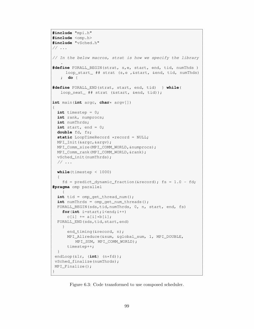
#include "mpi.h"#include <omp.h>#include "vSched.h"// ...
// In the below macros, strat is how we specify the library.
#define FORALL_BEGIN(strat, s,e, start, end, tid, numThds )loop_start_ ## strat (s,e ,&start, &end, tid, numThds)
; do {
#define FORALL_END(strat, start, end, tid) } while(loop_next_ ## strat (&start, &end, tid));
int main(int argc, char* argv[]){
int timestep = 0;int rank, numprocs;int numThrds;int start, end = 0;double fd, fs;static LoopTimeRecord *record = NULL;MPI_Init(&argc,&argv);MPI_Comm_size(MPI_COMM_WORLD,&numprocs);MPI_Comm_rank(MPI_COMM_WORLD,&rank);vSched_init(numThrds);// ...
while(timestep < 1000){
fd = predict_dynamic_fraction(&record); fs = 1.0 - fd;#pragma omp parallel
{int tid = omp_get_thread_num();int numThrds = omp_get_num_threads();FORALL_BEGIN(sds,tid,numThrds, 0, n, start, end, fs)
for(int i=start;i<end;i++)c[i] += a[i]*b[i];
FORALL_END(sds,tid,start,end)}
end_timing(&record, n);MPI_Allreduce(&sum, &global_sum, 1, MPI_DOUBLE,
MPI_SUM, MPI_COMM_WORLD);timestep++;
}endLoop(&lr, (int) (n*fd));vSched_finalize(numThrds);MPI_Finalize();
}
Figure 6.3: Code transformed to use composed scheduler.
99
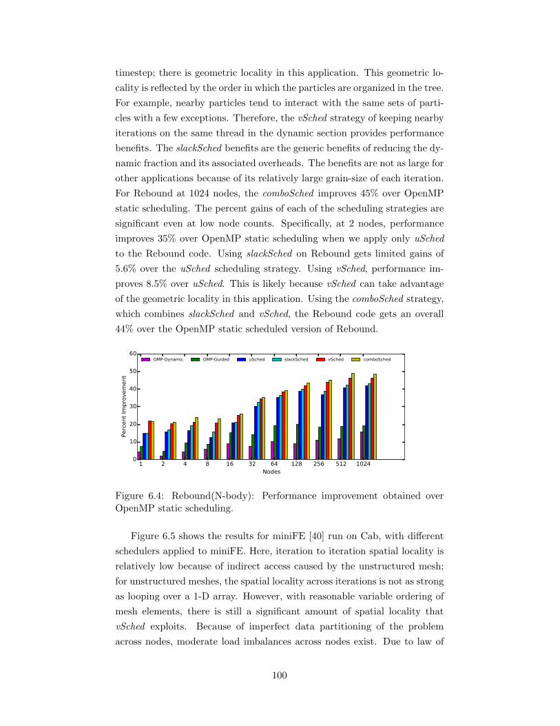
timestep; there is geometric locality in this application. This geometric lo-
cality is reflected by the order in which the particles are organized in the tree.
For example, nearby particles tend to interact with the same sets of parti-
cles with a few exceptions. Therefore, the vSched strategy of keeping nearby
iterations on the same thread in the dynamic section provides performance
benefits. The slackSched benefits are the generic benefits of reducing the dy-
namic fraction and its associated overheads. The benefits are not as large for
other applications because of its relatively large grain-size of each iteration.
For Rebound at 1024 nodes, the comboSched improves 45% over OpenMP
static scheduling. The percent gains of each of the scheduling strategies are
significant even at low node counts. Specifically, at 2 nodes, performance
improves 35% over OpenMP static scheduling when we apply only uSched
to the Rebound code. Using slackSched on Rebound gets limited gains of
5.6% over the uSched scheduling strategy. Using vSched, performance im-
proves 8.5% over uSched. This is likely because vSched can take advantage
of the geometric locality in this application. Using the comboSched strategy,
which combines slackSched and vSched, the Rebound code gets an overall
44% over the OpenMP static scheduled version of Rebound.
1 2 4 8 16 32 64 128 256 512 1024Nodes
0
10
20
30
40
50
60
Perc
ent
Impro
vem
ent
OMP-Dynamic OMP-Guided uSched slackSched vSched comboSched
Figure 6.4: Rebound(N-body): Performance improvement obtained overOpenMP static scheduling.
Figure 6.5 shows the results for miniFE [40] run on Cab, with different
schedulers applied to miniFE. Here, iteration to iteration spatial locality is
relatively low because of indirect access caused by the unstructured mesh;
for unstructured meshes, the spatial locality across iterations is not as strong
as looping over a 1-D array. However, with reasonable variable ordering of
mesh elements, there is still a significant amount of spatial locality that
vSched exploits. Because of imperfect data partitioning of the problem
across nodes, moderate load imbalances across nodes exist. Due to law of
100

large numbers, the imbalances across cores are larger at larger number of
nodes. Thus, dynamic and guided scheduling by itself should be able to pro-
vide significant performance gains. Consider the results for miniFE running
at 1024 nodes of Cab. The vSched scheduling strategy gets 15% perfor-
mance improvement over OpenMP static scheduling, while the slackSched
gets 19% performance gain over OpenMP static scheduling. The comboStrat
gets 23% performance improvement over OpenMP static scheduling, and
also gets 9.0% performance improvement over OpenMP guided scheduling.
By putting together vSched and slackSched, we are able to improve perfor-
mance further, to make our scheduling methodology perform better than
guided. The benefits of vSched and slackSched are not completely additive.
Composing the scheduling strategies along with tuning of parameters could
increase performance benefits, and could yield better performance for the
comboSched.
1 2 4 8 16 32 64 128 256 512 1024Nodes
0
10
20
30
40
50
60
Perc
ent
Impro
vem
ent
OMP-Dynamic OMP-Guided uSched slackSched vSched comboSched
Figure 6.5: miniFE (finite element): Performance improvement obtainedover OpenMP static scheduling.
Figure 6.6 shows the results for the regular mesh code SNAP [86] run
on Cab, with different schedulers applied to the SNAP code. The regular
mesh computation has no application load imbalance; the only load imbal-
ance during application execution is that due to noise. Note that the regular
mesh computation has inherent spatial locality (because the computation’s
sweep operation works on contiguous array elements). At 1024 nodes of
Cab, performance improves 10% over OpenMP static with slackSched, and
we get a reasonable performance gain of 16% over static scheduling with
vSched. The comboSched scheduler gets 19% performance improvement over
OpenMP static scheduling. This result of comboSched specifically helps to
show that the optimizations of vSched and slackSched composed in com-
boSched do not cancel out each other’s performance benefits, and that the
101
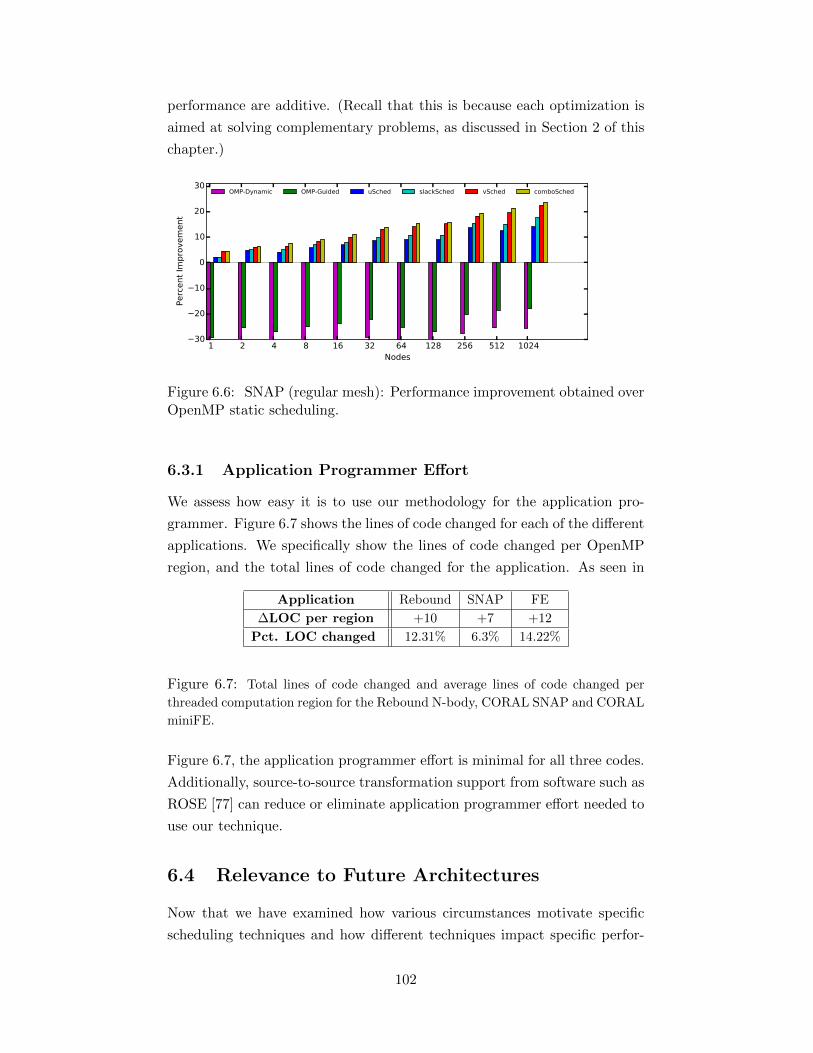
performance are additive. (Recall that this is because each optimization is
aimed at solving complementary problems, as discussed in Section 2 of this
chapter.)
1 2 4 8 16 32 64 128 256 512 1024Nodes
30
20
10
0
10
20
30Perc
ent
Impro
vem
ent
OMP-Dynamic OMP-Guided uSched slackSched vSched comboSched
Figure 6.6: SNAP (regular mesh): Performance improvement obtained overOpenMP static scheduling.
6.3.1 Application Programmer Effort
We assess how easy it is to use our methodology for the application pro-
grammer. Figure 6.7 shows the lines of code changed for each of the different
applications. We specifically show the lines of code changed per OpenMP
region, and the total lines of code changed for the application. As seen in
Application Rebound SNAP FE
∆LOC per region +10 +7 +12
Pct. LOC changed 12.31% 6.3% 14.22%
Figure 6.7: Total lines of code changed and average lines of code changed per
threaded computation region for the Rebound N-body, CORAL SNAP and CORAL
miniFE.
Figure 6.7, the application programmer effort is minimal for all three codes.
Additionally, source-to-source transformation support from software such as
ROSE [77] can reduce or eliminate application programmer effort needed to
use our technique.
6.4 Relevance to Future Architectures
Now that we have examined how various circumstances motivate specific
scheduling techniques and how different techniques impact specific perfor-
102
mance metrics, we examine the relevance of this work in the context of future
exascale machines.
As we go to exascale, the number of nodes in a parallel machine will
increase. This increases the likelihood of amplification. More importantly,
static and dynamic variability of future processor chips is likely to be much
higher. To complicate matters further, applications at exascale are likely to
be strong scaled [9]. Because of memory costs, the total amount of memory
will not increase as much as the number of FLOP/s. For example, the 10
petaflop MIRA, has about 0.8 petabytes of memory [88]. Summit, which
will be operational in 2017-2018, will have 15 times more floating-point per-
formance (150 PF), but only about 2.5 times more memory (2 PetaBytes).
This means the size of the problem in terms of memory will not increase
significantly, but it will have to be solved much faster to utilize this floating-
point capacity available. This is strong scaling. Separately, application
scientists are also increasingly seeking strong scaling. For many application
domains, scientists would want to solve the same problem faster rather than
a larger problem at the same speed.
Strong scaling implies that outer iteration durations for most applica-
tions will get smaller, e.g., of the order of a few milliseconds. We know
that for longer outer iterations, the impact of irregularities and noise-like
events can be absorbed without significant impact, but for shorter iterations,
the impact will be more significant. This raises the importance of dynamic
scheduling further. The locality cost differentials will also be higher in fu-
ture because of the large number of cores in a node, and necessarily deeper
memory hierarchy. Therefore, dynamic scheduling must be balanced care-
fully with locality considerations. Our scheduling strategies are designed to
handle exactly this balance.
Future machines will also have a large number of cores per node. These
may include heavier Xeon-like cores, or NVIDIA accelerator-like cores. Our
scheduling strategies are designed to utilize the abundance of cores to mit-
igate the scaling bottlenecks arising from variability, load imbalances, or
noise. So, our scheduling strategies distribute excess work on any core to
other cores, without significantly affecting locality.
Of course, exascale is still many years away. There will be many un-
known circumstances, in the combination of applications and architectures.
Yet, we have identified a large number of scheduling features in this work.
We expect many of the features to be relevant at exascale. Further, we have
demonstrated an extensible software infrastructure. We can combine the
features in different ways, as illustrated in this chapter. This extensibility,
103

combined with invention of new scheduling features inspired by specific ex-
ascale circumstances, will ensure that our approach will remain viable for
exascale.
104

Chapter 7
Related Work
The topics related to this dissertation research have received significant at-
tention by researchers in recent years. Some of the categories we discuss
in this chapter include noise and its amplification, MPI+X hybrid program-
ming, loop scheduling strategies, task scheduling strategies, dependent tasks,
cache-obliviousness, etc.
Several studies provide an in-depth analysis of noise and its impact on
large-scale systems [45, 68, 72, 82, 90]. Beckman et al. [8] discuss a bench-
mark for quantification of noise referred to as the selfish benchmark. This
benchmark has enabled a more accurate and proper study of noise in several
follow-up studies, and has allowed one to quantify noise on a system in a
standardized fashion.
The study by Petrini et al. of OS system services on ASCI Q inves-
tigates how to mitigate noise [72]. Noise mitigation is achieved through
system service suppression, i.e., the sources of system noise (in the form of
OS daemons) are identified, and then each non-critical service is stripped
away from the machine. Stripping away OS services was key to enabling
better performance of ASCI Q. They also suggest using co-scheduling to
make existing noise more coordinated. Furthermore, the study discusses
several lessons learned from their studies, particularly the impact that noise
mitigation solutions have on different classes of applications. The solutions
discussed in Petrini et al. are lower-level and specific to the platform used to
run the application. They are not portable to enable applicability to a larger
class of machines and a larger set of applications. As discussed in [54], a
higher-level solution is necessary to take advantage of the compute power of
emerging clusters of multi-cores. In particular, the application programmer
should have control over how the application should be implemented and
tuned, ensuring that characteristic noise has minimal impact on a particu-
lar problem. A paper discussing experimentation of a molecular dynamics
simulation code NAMD on a noisy system argues that effects of noise in the
communication sub-system can be mitigated by data-driven execution [73].
105
However, not all applications can use this technique. For some applications,
overlap of communication and computation is not possible due to inherent
strict dependencies across application time steps.
A study of the impact of noise for MPI applications was done by Hoefler
et al. [46]. This showed how noise can have a large impact for a particularly
large number of MPI processes. This assessment of performance loss is done
for several key scientific applications, and many different experiments are
carried out to understand changes in performance as the amount of system
noise is increased. Such studies have provided insight on how to mitigate
noise, and several studies show its usage.
An early study by Lusk with MPI+OpenMP focuses on the compar-
ison between MPI-everywhere and MPI+OpenMP codes [63]. Cappello
et al [19] show how MPI-everywhere performs better than MPI+OpenMP
codes. OpenMP has improved significantly since then, but some of the
issues still remain valid. The lack of locality-awareness in OpenMP pro-
gramming is the main reason for the performance problems. Rabenseifner
et al [78] provides an important introduction to the issues involved in hybrid
programming. They note that dynamic or guided loop scheduling is sub-
optimal because of its memory access performance, especially in a NUMA
context. We believe that the work in this thesis has addressed the challenge
referenced by this paper.
Application load balancing has been studied in [20, 47, 51]; these strate-
gies take advantage of the principle of persistence in load imbalance in
many applications. The problem with a system using measurement-based
load balancing on multi-core systems with transient load imbalance in-
duced by system noise is that it is difficult to predict the load imbalance in
each timestep. Thus, it is important to use a dynamic scheduling scheme
which reacts to changes in load during the application timestep, rather than
proactively assigning work to threads based on patterns in past application
timesteps. Load imbalances aren’t persistent across cores. The same goes
for Charm++ [51, 57] persistence across nodes, as these are uncoordinated
load imbalances.
Dynamic scheduling has been supported in OpenMP since the early days
of OpenMP [69]. Guided self-scheduling can reduce scheduler overhead com-
pared with it, while trying to maintain good load balance through exponen-
tially decreasing the chunk sizes [62,75] as threads execute chunks of work.
However, guided scheduling (along with other work-stealing schemes) may
not necessarily take into account outer iteration locality, or the temporal lo-
cality of data across application timesteps. This means that in one timestep,
106
the ith iteration is assigned to thread k, while in a subsequent timestep, the
ith iteration may be assigned to some other thread k′. Such patterns are
prevalent in a large number of HPC codes. In this work, the idea of the
tasklet aims to handle this outer iteration locality by storing within the
tasklet data structure a field denoting the last thread that the tasklet exe-
cuted on.
The work in Olivier et al. [71] discusses incorporation of affinity in
OpenMP scheduling for load imbalanced codes. This work considers op-
timizations specific to the OpenMP runtime. A key distinction between
our scheduling strategies and this work is that our method tunes the bal-
ance between locality and load imbalance for each application and architec-
ture rather than having a general runtime solution for handling locality for
scheduling. The importance of tuning the scheduler, given a particular ap-
plication and architecture, with the guidance of a simple model to validate
results, was shown in [27].
Chapman et al. [69] provide a system for OpenMP affinity-based lo-
cality parameters for each architecture, and finding the right placement of
data. This is done through detection of architecture parameters provided
in hardware. The system does not however tune to find the balancing of
scheduler overhead and load imbalance in an application, and also doesn’t
consider slack. Each combination of application and architecture can make
this tradeoff different, and tuning the application/architecture pairs provides
a solution that can handle the different tradeoffs.
Zhang et al. [47] describe an adaptive OpenMP loop scheduler that ad-
dresses synchronization and load imbalance issues that arise out of hyper-
threading (symmetric multi-threading), and it uses a NUMA-aware hierar-
chical scheduling strategy.
Loop iterations are a form of independent tasks. Several programming
models support creation of independent tasks directly. One of the key short-
comings of work-stealing [13,14,35] is that work-stealing incurs an overhead
due to the cost of a lock and the cost of coherence cache misses, both of
which depend on the number of cores and the shared memory interconnect
of the node architecture [18, 85]. Scalable work-stealing [25] is beneficial
in a distributed memory context, but it mainly focuses on steals across a
large number of nodes. We try to avoid the cost of overhead by doing
only within-node scheduling. Further work might include scheduling across
neighboring nodes. UPC scheduler [49] load imbalances across nodes are
not large enough to justify across node data movement.
SLAW (2010) [59] is a locality-aware scheduling scheme for Cilk. Its main
107
contribution is orthogonal to locality, a synthesis of work-first and help-first
scheduling. It addresses locality in a hierarchical sense, by dividing cores
into groups and prioritizing within-group steals first.
Threaded Building Blocks [80] use templates for common parallel itera-
tion patterns, written in terms of tasks, and supports dynamic load balanc-
ing.
Recently, many systems have started supporting creation of tasks that
depend on remote data as well as completion of other tasks. Examples
of such systems include DaGue and DPLASMA [15]. Galois for irregular
parallelism also represents a similar task creation mechanism [58]. These
scheduling strategies provide dynamic load balancing, but it is unclear if
they can address locality affectively. Concurrent Collections is another task
scheduling language that supports data-dependent and control-dependent
tasks [22] via graphs.
Much work has been done to improve scalability of bulk-synchronous
MPI applications on large-scale clusters of SMPs in the presence of the
changes in architectures and interconnect topologies [4, 87]. In the general
context of performance tuning of applications on multicore architectures,
several application papers investigate performance tuning of the applica-
tion timesteps for maximum efficiency in the compute phase of the bulk-
synchronous application. Some studies have aimed to find the best code
that maps to an architecture by enumerating the search space of all codes,
and then use machine learning to find the optimal code within the search
space [4, 55, 93]. Other application studies [19, 63, 78] on Hybrid Parallel
Programming have tried to document the techniques that programmers can
use to to harness the power of large-scale clusters through using a mixture of
different programming libraries. There are two main differences between the
approaches taken in the above work and the approach taken in this work.
First, each of these studies take a static approach and improve performance
locally within a node. In this work, we consider transient variations within
an SMP node, and maintain resiliency to unexpected noise on a core of a
node throughout the execution of the application. Second, these studies fo-
cus on the compute phase within one particular node, without consciousness
of MPI collective communication across nodes. In this work, we do consider
the collective communication for tuning the computation within each node.
The importance of spatial locality, specifically for static schedules, is dis-
cussed in [34,44], and also discussed in work demonstrating the importance
of block-cyclic data distributions [7, 76] in the context of static scheduling.
This work is complementary but orthogonal to our work, and we note that
108

it does not handle rearrangement or staggering of static and dynamic itera-
tions. In this work, we optimize for spatial locality through data placement
in the context of hybrid static/dynamic scheduling, as illustrated through
the use of a staggered approach.
109
Chapter 8
Conclusions
The broad problem that this thesis is concerned with is how to assign work
to compute elements in a synchronous data parallel program. Such a pro-
gram contains outer iterations, such as timesteps, and inner loop iterations,
typically over the data elements of the program. Application imbalances
arise when the time for different loop iterations are different. These im-
balances may be persistent or irregular. The machine imbalance could be
caused by noise, i.e., transient irregularities on specific cores, or it could be
persistent when some cores are slower than the others. Imbalances affect
performance of such programs significantly because all the processors wait
for the most loaded processor in every outer iteration.
One approach to solving this problem is to move data and work across
nodes. Typical MPI applications require an invasive reprogramming to do
this. This work focused on within-node load balancing. As we showed in
Chapter 1, given the large number of cores on each node, within-node load
balancing has a significant impact on global load imbalance, i.e., if you can
perfectly balance work within each node, much of the global imbalance will
be taken care of.
Although this seems like a straightforward solution, we demonstrated
that we are faced with three major challenges. While idle time can be
significantly reduced using OpenMP dynamic or guided scheduling, the syn-
chronization overhead, and data movement costs stop us from realizing the
full potential of this idea This work was aimed at developing scheduling
strategies the three challenges simultaneously, and demonstrates scalability
of applications to a large number of nodes.
Our basic approach is to fix a percentage of iterations that are exe-
cuted statically, and the remainder dynamically. The presence of a stati-
cally scheduled iterations helped to restore locality and reduce the above
synchronization and data movement costs to a much smaller level, while the
dynamically scheduled iteration allowed mitigation of load imbalance. This
design principle is carried out throughout this thesis.
110
Dynamically scheduled iterations add synchronization costs due to coor-
dination among thread to allocate iterations. More importantly, it disturbs
the locality in two different ways: (a) outer iteration locality: whether an
inner iteration continues to be scheduled on the same thread across outer
iterations, and (b) spatial locality within data parallel loops: whether con-
secutive inner iterations are executed consecutively on the same thread.
Both of these metrics are close to perfect with static scheduling, except that
it suffers from load imbalances. The series of strategies in the chapters can
be seen as increasingly sophisticated methods for improving both of these
locality factors.
In Chapter 2, we show how a careful selection of dynamic fraction, i.e.,
the percentage of iterations allocated dynamically improves performance
significantly. This was done in the context of both load imbalanced and load
balanced codes. This selection helps us balance the costs of idle time due
to imbalances and data movement overhead due to dynamic load balancing.
We showed the amplification problem arising from OS noise in the context
of a 3D regular mesh computation, analyzing it through histogramming of
outer iteration times, and how our strategy mitigates it. We also showed
how the scheduling of work benefits core computations in numerical linear
algebra, particularly dense matrix factorizations.
Chapter 3 showed how to schedule work given the persistent imbalance
observed among cores, typically because of high-frequency low-amplitude
noise events. This is done by changing the number of statically allocated
iterations to each thread, based on the recent history of outer iterations.
We also showed how to combine this weighted scheduling strategy with the
hybrid scheduling strategy of Chapter 2.
In Chapter 4, we showed how to reduce the search space for the dynamic
fraction through theoretical analysis coupled with a small runtime adjust-
ment. Further, by allowing the dynamic fraction to be different on different
MPI processes, we were able to take advantage of slack in MPI collective
operations, thus reducing the dynamic fraction further. This reduces the
dynamic scheduling overhead further, as demonstrated on multiple bench-
marks and application codes.
Although the previous techniques improve spatial locality and outer it-
eration locality in the static section, the dynamically scheduled iterations
lose the benefits of locality. By staggering the allocations of iteration space,
i.e., into alternate bands of statically and dynamically allocated iterations,
the dynamically scheduled iterations executed by a thread are made likely
to be contiguous to its statically scheduled iterations. This strategy was
111
described and demonstrated In Chapter 5.
Chapter 6 identified the problem that each of the performance issues ad-
dressed individually in previous chapters may exist together when running
applications on a cluster SMPs, notably for next-generation (most immi-
nently exascale) supercomputers. Given this, we showed an example com-
positions of our schedulers (developed in prior chapters), and showed, for
three representative MPI+OpenMP application codes, how this synthesis of
scheduling techniques can provide more performance benefits than that of
each of the individual schedulers that it was composed of.
Our runtime does not introduce significant overheads. Thus, even if
runtime slowdowns due to performance irregularity are negligible, it can
still be used, i.e., even when the user is unsure whether noise or imbalances
affect the application, they may use our scheduler without any concerns of
adding overhead.
Some specific ideas that immediately follow from this dissertation in-
clude the following: (a) the usage of our technique in MPI+X applica-
tions(including applications written with MPI-3 shared memory extensions),
as opposed to only MPI+OpenMP applications, and (b) developing addi-
tional examples of composite strategies and describing the circumstances
under which such strategies can be useful.
We showed how scheduling strategies within a node will be important in
the coming years as we get increasingly larger and more complex nodes. We
believe that our scheduling strategies, along with their potential for exten-
sion and composition, will contribute significantly to efficient utilization of
large-scale machines consisting of such nodes.
112
References
[1] Specifications of the MIRA Supercomputer. http://www.alcf.anl.gov/user-guides/mira-cetus-vesta, Jun 2011.
[2] Specifications of the Titan Supercomputer. https://www.olcf.ornl.gov/titan/, Oct 2012.
[3] L. Adhianto, S. Banerjee, M. Fagan, M. Krentel, G. Marin, J. Mellor-Crummey, and N. R. Tallent. HPCToolkit: Tools for Performance Anal-ysis of Optimized Parallel Programs. Concurrency and Computation:Practice and Experience, 22(6):685–701, 2010.
[4] D. H. Bailey, J. Chame, C. Chen, J. Dongarra, M. Hall, J. K.Hollingsworth, P. Hovland, S. Moore, K. Seymour, J. Shin, A. Tiwari,S. Williams, and H. You. PERI Auto-tuning. Journal of Physics: Con-ference Series, 125(1):012089, 2008.
[5] A. H. Baker, T. Gamblin, M. Schulz, and U. M. Yang. Challenges ofScaling Algebraic Multigrid Across Modern Multicore Architectures.IEEE International Parallel and Distributed Processing Symposium,pages 275–286, 2011.
[6] M. Bauer, S. Treichler, E. Slaughter, and A. Aiken. Legion: ExpressingLocality and Independence with Logical Regions. In Proceedings of theInternational Conference on High Performance Computing, Network-ing, Storage and Analysis, SC ’12, pages 66:1–66:11, Salt Lake City,UT, USA, 2012. IEEE Computer Society Press.
[7] D. Becker, M. Faverge, and J. Dongarra. Towards a Parallel Tile LDLFactorization for Multicore Architectures. Technical report, Universityof Tennessee at Knoxville, April 2011. ICL-UT-11-03.
[8] P. Beckman, K. Iskra, K. Yoshii, S. Coghlan, and A. Nataraj. Bench-marking the Effects of Operating System Interference on Extreme-scaleParallel Machines. Cluster Computing, 11:3–16, March 2008.
113

[9] K. Bergman, S. Borkar, D. Campbell, W. Carlson, W. Dally, M. Den-neau, P. Franzon, W. Harrod, J. Hiller, S. Karp, S. Keckler, D. Klein,R. Lucas, M. Richards, A. Scarpelli, S. Scott, A. Snavely, T. Ster-ling, R. S. Williams, K. Yelick, K. Bergman, S. Borkar, D. Campbell,W. Carlson, W. Dally, M. Denneau, P. Franzon, W. Harrod, J. Hiller,S. Keckler, D. Klein, P. Kogge, R. S. Williams, and K. Yelick. ExaScaleComputing Study: Technology Challenges in Achieving Exascale Sys-tems. Technical Report 0, University of Notre Dame, ComputationalScience and Engineering Department, September 2008.
[10] A. Bhatele, L. V. Kale, and S. Kumar. Dynamic Topology-Aware LoadBalancing Algorithms for Molecular Dynamics Applications. In 23rdACM International Conference on Supercomputing, ICS ’09, YorktownHeights, NY, USA, 2009. ACM.
[11] A. Bhatele, L. Wesolowski, E. Bohm, E. Solomonik, and L. V. Kale. Un-derstanding Application Performance via Micro-benchmarks on ThreeLarge Supercomputers: Intrepid, Ranger and Jaguar. InternationalJournal of High Performance Computing Applications (IJHPCA), 2010.http://hpc.sagepub.com/cgi/content/abstract/1094342010370603v1.
[12] A. Blanchard. Practical Experiences with OS Jitter. http://www.ibm.com/developerworks/wikis/display/LinuxP/OS+Jitter+Mitigation+Techniques, 2010.
[13] R. D. Blumofe, C. F. Joerg, B. C. Kuszmaul, C. E. Leiserson, K. H.Randall, and Y. Zhou. Cilk: An Efficient Multithreaded Runtime Sys-tem. In Journal of Parallel and Distributed Computing, 1995.
[14] R. D. Blumofe and C. E. Leiserson. Scheduling Multithreaded Compu-tations by Work Stealing. In In Proceedings of the 35th Annual Sym-posium on Foundations of Computer Science (FOCS), pages 356–368,Santa Fe, NM, USA, 1994.
[15] G. Bosilca, A. Bouteiller, A. Danalis, M. Faverge, A. Haidar,T. Herault, J. Kurzak, J. Langou, P. Lemarinier, H. Ltaief, P. Luszczek,A. Yarkhan, and J. J. Dongarra. Distibuted Dense Numerical LinearAlgebra Algorithms on Massively Parallel Architectures: DPLASMA.In Proceedings of the 25th IEEE International Symposium on Paralleland Distributed Processing Workshops and PhD Forum (IPDPSW’11),PDSEC 2011, pages 1432–1441, Anchorage, Alaska, USA, May 2011.
[16] F. Broquedis, J. Clet Ortega, S. Moreaud, N. Furmento, B. Goglin,G. Mercier, S. Thibault, and R. Namyst. hwloc: a Generic Frameworkfor Managing Hardware Affinities in HPC Applications. In PDP 2010 -The 18th Euromicro International Conference on Parallel, Distributedand Network-Based Computing, Pisa, Italy, 02 2010.
114

[17] S. Browne, J. Dongarra, N. Garner, G. Ho, and P. Mucci. A PortableProgramming Interface for Performance Evaluation on Modern Proces-sors. International Journal of High Performance Computing Applica-tions, 14(3):189–204, Aug. 2000.
[18] J. M. Bull. Measuring Synchronisation and Scheduling Overheads inOpenMP. In In Proceedings of First European Workshop on OpenMP,pages 99–105, Lund, Sweden, 1999.
[19] F. Cappello and D. Etiemble. MPI versus MPI+OpenMP on IBMSP for the NAS Benchmarks. In Proceedings of the 2000 ACM/IEEEconference on Supercomputing (CDROM), Supercomputing ’00, Dallas,TX, USA, 2000. IEEE Computer Society.
[20] U. Catalyurek, E. Boman, K. Devine, D. Bozdag, R. Heaphy, andL. Riesen. Hypergraph-based Dynamic Load Balancing for Adap-tive Scientific Computations. In IEEE International Parallel and Dis-tributed Processing Symposium, Long Beach, CA, USA, 2007. IEEE.
[21] E. Chan. Runtime Data Flow Scheduling of Matrix Computations.Technical Report FLAME Working Note 39, University of Texas atAustin, 2009.
[22] A. Chandramowlishwaran, K. Knobe, and R. Vuduc. Performance Eval-uation of Concurrent Collections on High-performance Multicore Com-puting Systems. In 2010 IEEE International Symposium on Paralleland Distributed Processing, pages 1–12, Atlanta, GA, USA, April 2010.
[23] L. Dagum and R. Menon. OpenMP: An Industry-Standard API forShared-Memory Programming. IEEE Computational Science & Engi-neering, 5(1), January-March 1998.
[24] J. Dempsey. i7-980x Details on Latencies of Caches and TLBand Buffers. https://software.intel.com/en-us/forums/topic/287236, June 2013.
[25] J. Dinan, D. B. Larkins, P. Sadayappan, S. Krishnamoorthy, andJ. Nieplocha. Scalable Work Stealing. In Proceedings of the Conferenceon High Performance Computing Networking, Storage and Analysis, SC’09, pages 53:1–53:11, Portland, OR, USA, 2009. ACM.
[26] S. Donfack, J. Dongarra, M. Faverge, M. Gates, and J. Kurzak. OnAlgorithmic Variants of Parallel Gaussian Elimination: Comparison ofImplementations in Terms of Performance and Numerical Properties,2013.
[27] S. Donfack, L. Grigori, W. D. Gropp, and V. Kale. Hybrid Static/Dy-namic Scheduling for Already Optimized Dense Matrix Factorizations.In IEEE International Parallel and Distributed Processing Symposium,IPDPS 2012, Shanghai, China, 2012.
115

[28] S. Donfack, L. Grigori, and A. Gupta. Adapting Communication-Avoiding LU and QR Factorizations to Multicore Architectures. In2010 IEEE International Parallel and Distributed Processing Sympo-sium, pages 1–10, Atlanta, GA, USA, April 2010.
[29] J. Dongarra, P. Beckman, T. Moore, P. Aerts, G. Aloisio, J.-C. An-dre, D. Barkai, J.-Y. Berthou, T. Boku, B. Braunschweig, F. Cap-pello, B. Chapman, X. Chi, A. Choudhary, S. Dosanjh, T. Dunning,S. Fiore, A. Geist, B. Gropp, R. Harrison, M. Hereld, M. Heroux,A. Hoisie, K. Hotta, Z. Jin, Y. Ishikawa, F. Johnson, S. Kale, R. Ken-way, D. Keyes, B. Kramer, J. Labarta, A. Lichnewsky, T. Lippert,B. Lucas, B. Maccabe, S. Matsuoka, P. Messina, P. Michielse, B. Mohr,M. S. Mueller, W. E. Nagel, H. Nakashima, M. E. Papka, D. Reed,M. Sato, E. Seidel, J. Shalf, D. Skinner, M. Snir, T. Sterling, R. Stevens,F. Streitz, B. Sugar, S. Sumimoto, W. Tang, J. Taylor, R. Thakur,A. Trefethen, M. Valero, A. Van Der Steen, J. Vetter, P. Williams,R. Wisniewski, and K. Yelick. The International Exascale SoftwareProject Roadmap. International Journal of High Performance Com-puting Applications, 25(1):3–60, Feb. 2011.
[30] P. Du, A. Bouteiller, G. Bosilca, T. Herault, and J. Dongarra.Algorithm-based Fault Tolerance for Dense Matrix Factorizations. SIG-PLAN Not., 47(8):225–234, Feb. 2012.
[31] A. E. Eichenberger, C. Terboven, M. Wong, and D. an Mey. The Designof OpenMP Thread Affinity. In International Workshop on OpenMP,pages 15–28, Rome, Italy, Jun 2012.
[32] A. Faraj, P. Patarasuk, and X. Yuan. A Study of Process ArrivalPatterns for MPI Collective Operations. In Proceedings of the 2006ACM/IEEE Conference on Supercomputing, SC ’06, Tampa, FL, USA,2006. ACM.
[33] E. Frachtenberg, D. G. Feitelson, F. Petrini, and J. Fernandez. AdaptiveParallel Job Scheduling with Flexible Coscheduling. IEEE Transactionsof Parallel and Distributed Systems, 16(11):1066–1077, Nov. 2005.
[34] M. Frigo, C. E. Leiserson, H. Prokop, and S. Ramachandran. Cache-Oblivious Algorithms. In Proceedings of the 40th Annual Symposium onFoundations of Computer Science, FOCS ’99, pages 285–, New York,NY, USA, 1999. IEEE Computer Society.
[35] M. Frigo, C. E. Leiserson, and K. H. Randall. The Implementationof the Cilk-5 Multithreaded Language. SIGPLAN Not., 33(5):212–223,May 1998.
[36] L. Grigori, J. Demmel, and H. Xiang. Communication-Avoiding Gaus-sian Elimination. In International Conference on High PerformanceComputing, Networking, Storage and Analysis, 2008. (SC 2008), pages1–12, Atlanta, GA, USA, Nov 2008.
116
[37] B. T. Gunney, A. M. Wissink, and D. A. Hysom. Parallel ClusteringAlgorithms for Structured AMR. Journal of Parallel and DistributedComputing, 66(11):1419 – 1430, 2006.
[38] J. Habich, C. Feichtinger, H. Kostler, G. Hager, and G. Wellein. Per-formance Engineering for the Lattice Boltzmann Method on GPGPUs:Architectural Requirements and Performance Results. Computers andFluids, abs/1112.0850, 2011.
[39] B. Hadri, H. Ltaief, E. Agullo, and J. Dongarra. Tall and Skinny QRMatrix Factorization Using Tile Algorithms on Multicore Architectures.Technical report, University of Tennessee at Knoxville, September 2009.ICL-UT-09-03.
[40] M. Heroux. MiniFE Documentation. http://www.nersc.gov/users/computational-systems/cori/nersc-8-procurement/trinity-nersc-8-rfp/nersc-8-trinity-benchmarks/minife/.
[41] J. Hess and A. Smith. Calculation of Potential Flow About ArbitraryBodies. Progress in Aerospace Sciences, 8(0):1 – 138, 1967.
[42] J. L. Hess. Panel Methods in Computational Fluid Dynamics. AnnualReview of Fluid Mechanics, 22:255–274, 1990.
[43] D. Hinkel, D. Callahan, N. Meezan, L. Suter, C. Still, D. Strozzi,E. Williams, and A. Langdon. Analyses of Laser-plasma Interactionsin NIF Ignition Emulator Designs. In Journal of Physics: ConferenceSeries, volume 244, page 022019. IOP Publishing, 2010.
[44] T. Hoefler, J. Dinan, D. Buntinas, P. Balaji, B. Barrett, R. Brightwell,W. Gropp, V. Kale, and R. Thakur. MPI + MPI: A New HybridApproach to Parallel Programming with MPI plus Shared Memory.Computing, 95(12):1121–1136, 2013.
[45] T. Hoefler, T. Schneider, and A. Lumsdaine. The Impact of NetworkNoise at Large-Scale Communication Performance. In Proceedings ofthe 23rd IEEE International Parallel & Distributed Processing Sympo-sium, LSPP’09 Workshop, Rome, Italy, May 2009.
[46] T. Hoefler, T. Schneider, and A. Lumsdaine. Characterizing the Influ-ence of System Noise on Large-Scale Applications by Simulation. InInternational Conference for High Performance Computing, Network-ing, Storage and Analysis (SC’10), New Orleans, LA, USA, Nov 2010.
[47] S. F. Hummel, J. Schmidt, R. N. Uma, and J. Wein. Load-sharing inHeterogeneous Systems via Weighted Factoring. In Proceedings of theEighth Annual ACM symposium on Parallel Algorithms and Architec-tures, SPAA ’96, pages 318–328, Padua, Italy, 1996. ACM.
[48] Intel. Intel Math Kernel Library. https://software.intel.com/en-us/intel-mkl/, 2011.
117
[49] S. jai Min, C. Iancu, and K. Yelick. Hierarchical Work Stealing onManycore Clusters. In In Fifth Conference on Partitioned Global Ad-dress Space Programming Models, New York, NY, USA, 2010.
[50] H. Jin and R. F. Van der Wijngaart. Performance Characteristics ofthe Multi-zone NAS Parallel Benchmarks. Journal of Parallel and Dis-tributed Computing, 66(5):674–685, May 2006.
[51] L. Kale and S. Krishnan. CHARM++: A Portable Concurrent ObjectOriented System Based on C++. In A. Paepcke, editor, Proceedings ofOOPSLA’93, pages 91–108. ACM Press, September 1993.
[52] V. Kale, A. Bhatele, and W. D. Gropp. Weighted Locality-SensitiveScheduling for Mitigating Noise on Multicore Clusters. In 18th An-nual IEEE International Conference on High Performance Computing(HiPC 2011), Bangalore, India, December 2011.
[53] V. Kale, S. Donfack, L. Grigori, and W. D. Gropp. Lightweight Schedul-ing for Balancing the Tradeoff Between Load Balance and Locality.2014.
[54] V. Kale and W. Gropp. Load Balancing for Regular Meshes on SMPswith MPI. In Proceedings of the 17th European MPI Users’ GroupMeeting Conference on Recent Advances in the Message Passing Inter-face, EuroMPI ’10, pages 229–238, Stuttgart, Germany, 2010. Springer-Verlag.
[55] S. Kamil, C. Chan, S. Williams, L. Oliker, J. Shalf, M. Howison, andE. W. Bethel. A Generalized Framework for Auto-tuning Stencil Com-putations. In In Proceedings of the Cray User Group Conference, 2009.
[56] T. Klug, M. Ott, J. Weidendorfer, C. Trinitis, and T. U. Mnchen. au-topin, Automated Optimization of Thread-to-Core Pinning on Multi-core Systems, 2008.
[57] S. Krishnan and L. V. Kale. Automating Runtime Optimizations forLoad Balancing in Irregular Problems. In Proc. Conf. on Paralleland Distributed Processing Technology and Applications, San Jose, CA,USA, August 1996.
[58] M. V. Kulkarni. The Galois System: Optimistic Parallelization of Ir-regular Programs. PhD thesis, Cornell University, 2008.
[59] V. Kumar, Y. Zheng, V. Cave, Z. Budimlic, and V. Sarkar. Habaner-oUPC: a Compiler-free PGAS Library, 2014.
[60] D. Levinthal. Intel Xeon Processor Architecture. https://software.intel.com/en-us/, Jun 2013.
[61] Y. D. Liu. Green Thieves in Work Stealing. In Seventeenth InternationalConference on Architectural Support for Programming Languages andOperating Systems, ASPLOS 2012, London, United Kingdom, 2012.
118
[62] S. E. Lucco. Adaptive Parallel Programs. PhD thesis, EECS Depart-ment, University of California, Berkeley, Aug 1994.
[63] E. Lusk and A. Chan. Early Experiments with the OpenMP/MPIHybrid Programming Model, 2004.
[64] E. Lusk, N. Doss, and A. Skjellum. A High-performance, PortableImplementation of the Message Passing Interface Standard. ParallelComputing, 22:789–828, 1996.
[65] P. D. V. Mann and U. Mittaly. Handling OS Jitter on Multicore Mul-tithreaded Systems. In Proceedings of the 2009 IEEE InternationalSymposium on Parallel and Distributed Processing Symposium, Rome,Italy, 2009. IEEE Computer Society.
[66] J. D. McCalpin. STREAM: Sustainable Memory Bandwidth in HighPerformance Computers. Technical report, University of Virginia,Charlottesville, VA, USA, 1991-2007. A continually updated techni-cal report.
[67] R. G. Minnich, M. J. Sottile, S.-E. Choi, E. Hendriks, and J. McKie.Right-weight Kernels: An off-the-shelf Alternative to Custom Light-weight Kernels. SIGOPS Oper. Syst. Rev., 40(2):22–28, Apr. 2006.
[68] A. Morari, R. Gioiosa, R. Wisniewski, F. J. Cazorla, and M. Valero. AQuantitative Analysis of OS Noise. In Proceedings of the IEEE Interna-tional Parallel and Distributed Processing Symposium, Anchorage, AK,USA, May 2011.
[69] A. Muddukrishna, P. A. Jonsson, V. Vlassov, and M. Brorsson.Locality-Aware Task Scheduling and Data Distribution on NUMA Sys-tems. In A. P. Rendell, B. M. Chapman, and M. Miller, editors,OpenMP in the Era of Low Power Devices and Accelerators, volume8122 of Lecture Notes in Computer Science, pages 156–170. SpringerBerlin Heidelberg, 2013.
[70] A. Nataraj, A. Morris, A. D. Malony, M. Sottile, and P. Beckman.The Ghost in the Machine: Observing the Effects of Kernel Opera-tion on Parallel Application Performance. In Proceedings of the 2007ACM/IEEE Conference on Supercomputing, pages 1–12, Reno, NV,USA, 2007. ACM.
[71] S. L. Olivier, B. R. de Supinski, M. Schulz, and J. F. Prins. Character-izing and Mitigating Work Time Inflation in Task Parallel Programs. InProceedings of the International Conference on High Performance Com-puting, Networking, Storage and Analysis, SC ’12, pages 65:1–65:12,Salt Lake City, UT, USA, 2012. IEEE Computer Society Press.
119
[72] F. Petrini, D. J. Kerbyson, and S. Pakin. The Case of the MissingSupercomputer Performance: Achieving Optimal Performance on the8,192 Processors of ASCI Q. In Proceedings of the 2003 ACM/IEEEConference on Supercomputing, Phoenix, AZ, USA, 2003. IEEE Com-puter Society.
[73] J. C. Phillips, G. Zheng, S. Kumar, and L. V. Kale. NAMD: Biomolec-ular simulation on thousands of processors. In Proceedings of the 2002ACM/IEEE Conference on Supercomputing, pages 1–18, Baltimore,MD, USA, September 2002.
[74] T. Pohl, F. Deserno, N. Thurey, U. Rude, P. Lammers, G. Wellein,and T. Zeiser. Performance Evaluation of Parallel Large-Scale LatticeBoltzmann Applications on Three Supercomputing Architectures. InProceedings of the 2004 ACM/IEEE Conference on Supercomputing,SC ’04, Pittsburgh, PA, USA, Nov 2004. IEEE Computer Society.
[75] C. D. Polychronopoulos and D. J. Kuck. Guided Self-scheduling: APractical Scheduling Scheme for Parallel Supercomputers. IEEE Trans-actions of Computing, 36:1425–1439, December 1987.
[76] L. Prylli and B. Tourancheau. Fast Runtime Block Cyclic Data Re-distribution on Multiprocessors. Journal of Parallel and DistributedComputing, 45(1):63 – 72, 1997.
[77] D. Quinlan. ROSE: Compiler Support for Object-Oriented Frameworks.Parallel Processing Letters, 10, January 2000.
[78] R. Rabenseifner. Hybrid Parallel Programming: Performance Problemsand Chances. In In Proceedings of the Forty-Fifth Cray User’s GroupConference, Columbus, OH, USA, May 2003.
[79] H. Rein and S. F. Liu. REBOUND: An Open-source Multi-purposeN-body Code for Collisional Dynamics. Astronomy and Astrophysics,537:A128, 2012.
[80] J. Reinders. Intel Threading Building Blocks: Outfitting C++ for Multi-Core Processor Parallelism. O’Reilly Media, 2007.
[81] B. Rountree, D. K. Lowenthal, B. R. de Supinski, M. Schulz, V. W.Freeh, and T. Bletsch. Adagio: Making DVS Practical for ComplexHPC Applications. In Proceedings of the 23rd International Conferenceon Supercomputing, ICS ’09, pages 460–469, Yorktown Heights, NY,USA, 2009. ACM.
[82] S. Seelam, L. Fong, A. Tantawi, J. Lewars, J. Divirgilio, and K. Gildea.Extreme-scale Computing: Modeling the Impact of System Noise inMulticore Clustered Systems. In Proceedings of the IEEE InternationalParallel and Distributed Processing Symposium, pages 1–12, Atlanta,GA, USA, April 2010.
120
[83] J. R. Shewchuk. Triangle: Engineering a 2D Quality Mesh Genera-tor and Delaunay Triangulator. In M. C. Lin and D. Manocha, edi-tors, Applied Computational Geometry: Towards Geometric Engineer-ing, volume 1148 of Lecture Notes in Computer Science, pages 203–222.Springer-Verlag, May 1996. From the First ACM Workshop on AppliedComputational Geometry.
[84] F. Song, A. YarKhan, and J. Dongarra. Dynamic Task Scheduling forLinear Algebra Algorithms on Distributed-Memory Multicore Systems.In Proceedings of the Conference on High Performance Computing Net-working, Storage and Analysis, Portland, OR, USA, 2009. ACM.
[85] P. Stenstrom. A Survey of Cache Coherence Schemes for Multiproces-sors. Computer, 23(6):12–24, June 1990.
[86] A. Talamo. Numerical Solution of the Time Dependent Neutron Trans-port Equation by the Method of the Characteristics. Journal of Com-putational Physics, 240(0):248 – 267, 2013.
[87] Y. Tang, R. A. Chowdhury, B. C. Kuszmaul, C.-K. Luk, and C. E. Leis-erson. The Pochoir Stencil Compiler. In Proceedings of the Twenty-thirdAnnual ACM Symposium on Parallelism in Algorithms and Architec-tures, SPAA ’11, pages 117–128, San Jose, CA, USA, 2011. ACM.
[88] T. Trader. Obamas 2016 Budget Boosts R & D Exas-cale Funding. http://www.hpcwire.com/2015/02/04/obamas-2016-budget-request-holds-clues-exascale/.
[89] L. N. Trefethen and I. David Bau. Numerical Linear Algebra.
[90] D. Tsafrir, Y. Etsion, D. G. Feitelson, and S. Kirkpatrick. System Noise,OS Clock Ticks, and Fine-grained Parallel Applications. In Proceedingsof the 19th annual international conference on Supercomputing, ICS’05, pages 303–312, Cambridge, MA, USA, 2005. ACM.
[91] S. Vetter. Architecture of the IBM POWER7+ Technology-Based IBMPower 750 and IBM Power 760. http://www.redbooks.ibm.com/Redbooks.nsf/RedbookAbstracts/tips0972.html, Feb. 2013.
[92] M. S. Warren and J. K. Salmon. A Parallel Hashed Oct-Tree N-bodyAlgorithm. In Proceedings of the 1993 ACM/IEEE Conference on Su-percomputing, SC ’93, pages 12–21, Portland, OR, USA, 1993. ACM.
[93] S. Williams, J. Carter, L. Oliker, J. Shalf, and K. A. Yelick. Optimiza-tion of a Lattice Boltzmann Computation on State-of-The-art MulticorePlatforms. Journal of Parallel and Distributed Computing, 2009.
[94] G. Zheng. Achieving High Performance on Extremely Large ParallelMachines: Performance Prediction and Load Balancing. PhD the-sis, Department of Computer Science, University of Illinois at Urbana-Champaign, 2005.
121