c 2015, thomas m. halverson
TRANSCRIPT
Exact Quantum Dynamics Calculations of Large Dimensional Molecules UsingPhase Space Basis Truncation
by
Thomas M. Halverson, B.S.
A Dissertation
In
PHYSICS
Submitted to the Graduate Facultyof Texas Tech University in
Partial Fulfillment ofthe Requirements for
the Degree of
DOCTOR OF PHILOSOPHY
Dr. L. William (Bill) PoirierChairperson of the Committee
Dr. Jorge A. Morales
Dr. Thomas L. Gibson
Dr. Mahdi Sanati
Dr. Mark SheridanDean of the Graduate School
December 2015

c©2015, Thomas M. Halverson

Texas Tech University, Thomas M. Halverson, December 2015
ACKNOWLEDGEMENTS
This work was largely supported by a grant from The Robert A. Welch Founda-
tion (D-1523). In addition, both a research grant (CHE-1012662) and a CRIF MU
instrumentation grant (CHE-0840493) from the National Science Foundation are ac-
knowledged. I also gratefully acknowledge the following entities for providing access
and technical support for their respective computing clusters: the Texas Tech Univer-
sity High Performance Computing Center, for use of the Hrothgar facility; the Texas
Tech University Department of Chemistry and Biochemistry, for use of the Robinson
cluster; the Texas Advanced Computing Center, for use of the Lonestar 4 facility. Cal-
culations presented in this paper were performed using the SwitchBLADE parallel
code.
Despite doing most of the research present here on my own, many people pro-
vided invaluable contributions indirectly. Firstly, I would like to thank my adviser,
Dr. Bill Poirier, without whom I would still be aimlessly wandering the physics land-
scape. His tutelage and guidance has made me not only a better scientist, but also a
better person. Secondly, none of this would have been possible with out the endless
help from my colleague, Dr. Corey Petty. In our countless discussions, he proved
time and again to be an invaluable source of advice (and criticism when needed).
Moreover, his technological knowledge, combined with his immense patience, kept
me sane throughout this entire process. Lastly, I would like to thank my mother and
sister, whose love and support was always in the background keeping me on course.
ii

Texas Tech University, Thomas M. Halverson, December 2015
TABLE OF CONTENTS
Acknowledgements . . . . . . . . . . . . . . . . . . . . . . . . . . . . . . . ii
Abstract . . . . . . . . . . . . . . . . . . . . . . . . . . . . . . . . . . . . . v
List of Tables . . . . . . . . . . . . . . . . . . . . . . . . . . . . . . . . . . vi
List of Figures . . . . . . . . . . . . . . . . . . . . . . . . . . . . . . . . . . viii
Acronyms . . . . . . . . . . . . . . . . . . . . . . . . . . . . . . . . . . . . ix
1. Introduction . . . . . . . . . . . . . . . . . . . . . . . . . . . . . . . . . 1
2. Theory . . . . . . . . . . . . . . . . . . . . . . . . . . . . . . . . . . . . 5
2.1 Problem Overview . . . . . . . . . . . . . . . . . . . . . . . . . 5
2.2 The Phase Space Picture . . . . . . . . . . . . . . . . . . . . . 6
2.3 The Symmetrized Gaussian Basis Set . . . . . . . . . . . . . . 10
2.4 The Harmonic Oscillator Basis Set (revisited) . . . . . . . . . . 14
3. SwitchBLADE and Computational Scaling . . . . . . . . . . . . . . . 26
3.1 Version 1.0 . . . . . . . . . . . . . . . . . . . . . . . . . . . . . 27
3.2 Version 2.0 . . . . . . . . . . . . . . . . . . . . . . . . . . . . . 29
3.3 Advanced Search Algorithms (Sherlock v1.0) . . . . . . . . . . 32
3.4 GHOST Module . . . . . . . . . . . . . . . . . . . . . . . . . . 35
4. Dimensional Scaling and Proof of Concept . . . . . . . . . . . . . . . . 39
4.1 Isotropic Uncoupled Harmonic Oscillators (IUHO’s) . . . . . . 39
4.2 Coupled Anharmonic Oscillators (CAHO’s) . . . . . . . . . . . 44
4.2.1 Two-dimensional case (D = 2) . . . . . . . . . . . . . . . . 45
4.2.2 Three-dimensional case (D = 3) . . . . . . . . . . . . . . . 48
4.2.3 Four-dimensional case (D = 4) . . . . . . . . . . . . . . . . 48
4.2.4 Accurate numerical convergence study: D = 3 revisited . . 49
4.2.5 Eight-, twelve-, and sixteen-dimensional cases (D = 8, D =
12, and D = 16) . . . . . . . . . . . . . . . . . . . . . . . . 53
4.3 Conclusions . . . . . . . . . . . . . . . . . . . . . . . . . . . . 55
5. Diphosphorous Oxide (D = 3) . . . . . . . . . . . . . . . . . . . . . . . 59
6. Methyleneimine (D = 9) . . . . . . . . . . . . . . . . . . . . . . . . . . 64
7. Acetonitrile (D = 12) . . . . . . . . . . . . . . . . . . . . . . . . . . . . 69
7.1 Force Field Potential . . . . . . . . . . . . . . . . . . . . . . . 69
iii

Texas Tech University, Thomas M. Halverson, December 2015
7.2 Results . . . . . . . . . . . . . . . . . . . . . . . . . . . . . . . 73
7.3 Conclusions . . . . . . . . . . . . . . . . . . . . . . . . . . . . 75
8. Benzene (D = 30) . . . . . . . . . . . . . . . . . . . . . . . . . . . . . . 79
8.1 Low-lying energy levels . . . . . . . . . . . . . . . . . . . . . . 82
8.2 High-lying energy levels . . . . . . . . . . . . . . . . . . . . . . 84
8.3 Hybrid Truncation (HT) dataset . . . . . . . . . . . . . . . . . 86
8.4 Conclusions . . . . . . . . . . . . . . . . . . . . . . . . . . . . 88
9. Closing Remarks . . . . . . . . . . . . . . . . . . . . . . . . . . . . . . . 105
References . . . . . . . . . . . . . . . . . . . . . . . . . . . . . . . . . . . . 108
iv

Texas Tech University, Thomas M. Halverson, December 2015
ABSTRACT
Over the course of this project, a simple, stand-alone software code was devel-
oped, using Fortran 90 and MPI, to compute the exact vibrational spectrum of
molecular systems. This code, named SwitchBLADE, is dimensionally independent
and, therefore, can be used for a myriad of different molecular systems. A full theo-
retical analysis of what makes SwitchBLADE possible is presented—i.e., the phase
space truncated symmetrized Gaussian basis and the energy truncated harmonic os-
cillator basis. Moreover, a full discussion of how phase space arguments can be used
to better improve these truncation techniques is given. Also presented are vibrational
spectra for isotropic uncoupled harmonic oscillators, coupled anharmonic oscillators,
diphosphorous oxide (P2O), methyleneimine (CH2NH), acetonitrile (CH3CN), and
benzene (C6H6), all of which were computed using the same SwitchBLADE code.
The full dynamically relevant range of states for each spectra is presented, which
varies from a few hundred for P2O to over one million for C6H6.
v

Texas Tech University, Thomas M. Halverson, December 2015
LIST OF TABLES
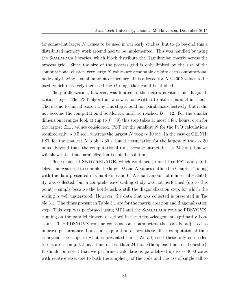
3.1 SwitchBLADE Computational Scaling Data . . . . . . . . . . . . . 32
3.2 Numerical performance of GHOST: Creation vs. diagonalization . . . 37
3.3 Numerical performance of GHOST: Total runtime . . . . . . . . . . . 38
4.1 Number of accurately computed states for D = 5 . . . . . . . . . . . 41
4.2 Number of accurately computed states for D = 6 . . . . . . . . . . . 42
4.3 Number of accurately computed states for D = 7 . . . . . . . . . . . 42
4.4 Number of accurately computed states for D = 8 . . . . . . . . . . . 42
4.5 Number of accurately computed states for D = 9, D = 10, and D = 11 43
4.6 Number of accurately computed states for D = 12 to D = 19 . . . . . 44
4.7 Number of accurately computed states for D = 12 to D = 27 using
parallel implementation . . . . . . . . . . . . . . . . . . . . . . . . . . 45
4.8 Selected computed eigenvalues forD = 3 coupled anharmonic oscillator
(CAHO) . . . . . . . . . . . . . . . . . . . . . . . . . . . . . . . . . . 51
4.9 Comparison between the number of accurate states computed using
µ = 0.0 HOB and SGB, for the D = 3 coupled anharmonic oscillator . 53
4.10 Number of accurate states computed for D = 8, D = 12, and D = 16
coupled anharmonic oscillators . . . . . . . . . . . . . . . . . . . . . . 55
5.1 Vibrational spectra for P2O . . . . . . . . . . . . . . . . . . . . . . . 62
5.2 Selected computed energy eigenvalues for P2O . . . . . . . . . . . . . 63
5.3 Number of converged energy eigenstates for P2O . . . . . . . . . . . . 63
6.1 Selected computed energy eigenvalues for CH2NH . . . . . . . . . . . 67
6.2 Number of converged energy eigenstates for CH2NH . . . . . . . . . . 67
7.1 Basis sizes for CH3CN . . . . . . . . . . . . . . . . . . . . . . . . . . 70
7.2 Comparison of selected computed eigenfrequencies for CH3CN . . . . 78
8.1 Normal mode frequencies for C6H6 . . . . . . . . . . . . . . . . . . . 80
8.2 Basis sizes for C6H6 . . . . . . . . . . . . . . . . . . . . . . . . . . . . 82
8.3 Lowest 34 eigenfreqencies of the A1g ⊕ E2gx block of C6H6 . . . . . . 92
8.4 Lowest 26 eigenfrequencies of the A2g ⊕ E2gy block of C6H6 . . . . . . 93
8.5 Lowest 33 eigenfrequencies of the B1u ⊕ E1ux block of C6H6 . . . . . . 94
8.6 Lowest 34 eigenfrequencies of the B2u ⊕ E1uy block of C6H6 . . . . . . 95
vi

Texas Tech University, Thomas M. Halverson, December 2015
8.7 Lowest 29 eigenfrequencies of the B1g ⊕ E1gx block of C6H6 . . . . . . 96
8.8 Lowest 35 eigenfrequencies of the B2g ⊕ E1gy block of C6H6 . . . . . . 97
8.9 Lowest 31 eigenfrequencies of the A1u ⊕ E2ux block of C6H6 . . . . . . 98
8.10 Lowest 35 eigenfrequencies of the A2u ⊕ E2uy block of C6H6 . . . . . . 99
8.11 Comparison of selected frequencies for C6H6 . . . . . . . . . . . . . . 100
8.12 Number of converged eigenstates for C6H6, using µ = 0.1 . . . . . . . 101
8.13 Number of converged eigenstates for C6H6, using µ = 0.1 . . . . . . . 101
8.14 Number of converged eigenstates for C6H6, using µ = 1.0 . . . . . . . 102
8.15 Number of states chosen during the hybrid process . . . . . . . . . . 102
8.16 Selected frequencies for C6H6using hybrid truncation . . . . . . . . . 103
8.17 Number of converged eigenstates for C6H6, using hybrid truncation . 104
vii

Texas Tech University, Thomas M. Halverson, December 2015
LIST OF FIGURES
2.1 Phase space contours: HOB vs. SGB . . . . . . . . . . . . . . . . . . 8
2.2 Schematic representation of the P2O potential energy . . . . . . . . . 9
2.3 Short range ρK for h(2) . . . . . . . . . . . . . . . . . . . . . . . . . . 17
2.4 Short range ρN for h(2) using polyad truncation . . . . . . . . . . . . 18
2.5 Short range ρN for h(2) using frequency truncation . . . . . . . . . . . 19
2.6 Long range ρK for h(2) . . . . . . . . . . . . . . . . . . . . . . . . . . 20
2.7 Long range ρN for h(2) using polyad truncation . . . . . . . . . . . . . 21
2.8 Long range ρN for h(2) using frequency truncation . . . . . . . . . . . 21
3.1 Schematic representation of Sherlock algorithm . . . . . . . . . . . 34
3.2 SwitchBLADE: Schematic overview . . . . . . . . . . . . . . . . . . 36
4.1 Lowest 50 computed states for D = 2 coupled anharmonic oscillator . 47
4.2 Lowest 150 computed states for D = 3 coupled anharmonic oscillator 49
4.3 Lowest 400 computed states for D = 4 coupled anharmonic oscillator 50
4.4 Lowest 105 computed states for D = 3 CAHO . . . . . . . . . . . . . 58
6.1 Contour plot of the q1 and q7 normal mode coordinates for CH2NH . 65
6.2 Reaction profile corresponding to the CH2NH dissociation reaction path 66
7.1 Reaction profiles for the C–C stretch of CH3CN . . . . . . . . . . . . 71
7.2 Errors of selected computed eigenfrequencies for CH3CN . . . . . . . 75
viii
Texas Tech University, Thomas M. Halverson, December 2015
ACRONYMS
CAHO coupled anharmonic oscillator. 2, 28, 44, 47, 49–55, 58, 105
D dimensionality. 1–6, 8, 9, 21, 22, 24, 26, 28, 30–32, 39–41, 46, 48, 49, 52–57, 59,
60, 68, 69, 76, 86, 88–90, 106
D&H Davis and Heller. 1, 8, 10, 12
DPB direct product basis. 1, 3, 5, 6, 9, 15, 76
DVR discrete variable representation. 3, 4, 29, 59, 89
E0 the ground state energy. 3, 52, 62, 63, 66, 69, 73, 86
EQD exact quantum dynamics. 1, 2, 9, 26, 35, 39, 64, 70, 74, 76, 77, 88, 89
FFP force field potential. 2–5, 7, 13, 16, 26, 29, 30, 33, 59, 60, 64, 69–74, 77, 79–81,
83, 90, 91, 105–107
FT frequency truncation. 16–22
HOB harmonic oscillator basis. 2, 6, 8–10, 14–16, 18–21, 23, 24, 26, 35, 45, 50–53,
58–60, 66, 68, 69, 71–73, 77, 81, 88–90, 106
HT hybrid truncation. 23, 53, 73, 86–88, 90
IUHO isotropic uncoupled harmonic oscillator. 2, 3, 27, 39, 41–48, 50, 54, 105
K total number of converged states. 3, 7–9, 15, 18, 20, 39–41, 46, 57, 86, 88–90
L dynamically relevant states. 3, 4, 46, 60, 84
MCTDH multi-configuration time dependent Hartree. 57
N basis size. 1, 5–7, 15, 16, 20, 22–24, 27, 28, 30, 31, 36, 37, 39–41, 44, 46, 50–54,
56, 57, 68–70, 73, 81, 82, 85, 86, 89, 90
ix

Texas Tech University, Thomas M. Halverson, December 2015
PDF phase space quasi-probability density function. 7, 15–21
PertT perturbation theory. 3, 28, 45–50, 53, 79, 83, 84
PES potential energy surface. 2, 6, 52, 56, 57, 77, 79, 90, 91, 106
PSLB phase space localized basis. 8–10, 59, 61, 69, 88, 90, 105
PSP phase space picture. 6, 14, 15, 17–19, 26, 76, 77, 79, 84, 88–91, 106
PSRO phase space region operator. 56, 57, 90, 106, 107
PST phase space truncation. 7, 8, 10–12, 27–32, 35, 39, 56, 59, 61, 68, 105
PT polyad truncation. 16–18, 20–22, 85
SGB symmetrized Gaussian basis. 2, 8, 12–14, 24, 26–28, 30, 35, 39–53, 55–66,
68–71, 73, 74, 76–78, 81, 105
x

Texas Tech University, Thomas M. Halverson, December 2015
CHAPTER 1
INTRODUCTION
The calculation of numerically exact nuclear rovibrational eigenstates [what we
call exact quantum dynamics (EQD)]1 for large molecules has been considered a
“holy grail” of chemical physics for some time. The major hindrance preventing
progress in this area has always been the exponential scaling of the computational
basis size (N) with respect to the dimensionality (D) of the problem.2–6 That is
to say that as D increases, the N needed to maintain a constant level of accuracy
grows exponentially and, therefore, reaches a size where direct computation of the
eigenvectors and eigenvalues of the Hamiltonian matrix becomes impractical (if not
impossible). This is, of course, an artifact of using a direct product basis (DPB)—i.e.,
expressing the multidimensional basis functions as direct products of single variable
basis functions. In the past few years, massively parallelized computational platforms
(with total number of process cores reaching ∼ 105) have pushed the limits of what
was possible in this regard, but on its own parallelization does not directly address the
exponential scaling issue. Alongside the computational developments, many methods
have been developed that attempt to side-step this so-called “curse of dimensionality”
by either utilizing some sort of basis truncation—decreasing N to a point where
computational diagonalization is possible, without sacrificing the basis efficacy—or by
utilizing innovative techniques for the matrix diagonalization process, e.g. iterative
methods.3,7? –17 Although the latter is useful and ultimately, combing both ideas
would be the end goal, the former is where the research contained herein is focused.
In particular, we present a phase space based methodology that not only explains
the causes of exponential scaling, but also provides a direct solution to this long
standing problem. The method was derived by piggybacking on previous work done
in 1979 by Davis and Heller (D&H), whereby they attempted to utilize a rectilinear
lattice of phase space Gaussians truncated using the classical Hamiltonian energy.18
This original attempt ultimately failed, but by building on this seminal work, Poirier
and coworkers were able to devise the first basis that formally defeats exponential
scaling—momentum symmetrized weylets.19–21 Although the work contained herein
does not directly use momentum symmetrized weylets, owing to their complexity,
1

Texas Tech University, Thomas M. Halverson, December 2015
it does utilize a simplified version—i.e., the symmetrized Gaussian basis (SGB)—
which has been shown to be as efficient despite being non-orthogonol.22 Moreover,
the SGB still retains the properties necessary to defeat exponential scaling. Along
with results obtained by using the SGB, we also utilize phase space based arguments
to systematically explore different truncation methods for the harmonic oscillator
basis (HOB). In essence, this yields a problem specific methodology that works in
conjunction with the SGB to dramatically improve computational accuracy, especially
in the lower energy regime.
Traditionally, any EQD problem can be broken down into three components: (1)
performing electronic structure calculations over a wide range of nuclear configura-
tions to produce a potential energy surface (PES); (2) choosing a suitable basis set
in which to expand the (ro)vibirational Hamiltonian; and (3) diagonalizing the re-
sultant Hamiltonian matrix via some numerical technique. Density functional theory
and ab intio methods have made (1) a relatively simple, everyday occurrence even for
systems of very large D.23 In fact, many “black-box” software packages have become
available for the calculation of electronic structure (e.g. Gaussian24). However, this
is not the case for (2) and (3), mainly due to the aforementioned “curse of dimension-
ality”. In that vein, we present results obtained from a software package designed for
such a purpose. Using Fortran 90, Scalapack, and MPI, we have developed a
simple, black-box code, featuring Switchable Basis set Linear Algebra modules for
Dimensionally independent Eigensolves—“SwitchBLADE”. This new code com-
putes bound vibrational energy levels and wavefunctions for virtually any molecule
for which the PES is expressed as a fourth order polynomial—i.e., a force field po-
tential (FFP). As a proof of concept for the underlying methodology, the vibrational
spectra of isotropic uncoupled harmonic oscillator (IUHO) systems and CAHO sys-
tems, ranging from D= 5 to D= 27, are presented. These initial calculations serve
as a reliable benchmark for the both the accuracy limitations and the dimensional
scaling of SwitchBLADE. To add to this, the vibrational spectra of diphosphorous
oxide (P2O), D= 3, and methyleneimine (CH2NH), D= 9, were computed to show-
case the viability of SwitchBLADE in the context of realistic molecular systems.
Lastly, the vibrational spectra of acetonitrile (CH3CN), D=12, and benzene (C6H6),
D= 30 are presented. These last two molecular systems, CH3CN and C6H6, repre-
2

Texas Tech University, Thomas M. Halverson, December 2015
sent some of the largest systems, in terms of D, ever studied exactly, and without a
“smart” methodology, calculations of this size would not even be possible, especially
in a “black-box” manner.
With respect to accuracy, there are several different methods by which it can be
judged. The most obvious is a simple comparison between the calculated results and
“known” results—i.e. comparing the results of the new theoretical model to that of
a more typical theoretical calculation, like perturbation theory (PertT). The draw-
back here is that the overall goal of this project is to compute states that lie very
high in energy, where mode coupling and anharmonicities are strongly represented.
This is, of course, where PertT begins to break down, making direct comparison
dubious at best. Moreover, other traditional methods, e.g. discrete variable repre-
sentation (DVR),3,5,9,25–31 suffer immensely from dimensional scaling vis-a-vis their
use of DPB’s. Hence, they are very rarely used to study systems of large D, and
when they are utilized, they do not report a very large total number of converged
states (K), usually no more than K = 103. On the contrary, if we wish to compute
all of the dynamically relevant states (L)—i.e, all states that lie below ∼ 5000–6000
cm−1 above the ground state energy (E0), which for large molecules (D = 10−30)
can be on the order of L= 105—then we must look elsewhere. A second test would
be intramethod comparison—i.e., comparing the results from one calculations done
using N1 to another calculation done using N2, where N1 > N2. Of course, this
is predicated on the method being variational, in which case all computed eigenval-
ues converge from above. Since SwitchBLADE uses analytic matrix elements and
an analytic FFP, it yields computed eigenvalues that are strictly variational and is,
therefore, amenable to this form of analysis. However, more recent developments
have yielded a new method by which accuracy can be assessed—intermethod. Given
two calculations from two separate methods using the same FFP where N1 ≈ N2,
the method that yields the lowest lying eigenvalues is the most accurate. This sort of
analysis has proven to be very fruitful in cases where D is so large that a converged
E0 is difficult to compute. For the results presented here, all three methods were
utilized, where applicable, along with comparison to analytic solutions (in the case of
the model IUHO).
3

Texas Tech University, Thomas M. Halverson, December 2015
It should be noted that in its current implementation, SwitchBLADE has one
major drawback—overall accuracy. More traditional methods (like DVR) are able to
compute states to sub-wavenumber convergence—i.e., spectroscopic accuracy. The
major drawback is that the spectrum is computed a few states at a time. For systems
of large D, computing all of L in this manner becomes intractable. SwitchBLADE,
on the other hand, computes the entire spectrum in one calculation, since it utilizes
direct diagonalization methods. The trade-off being the highest-lying states are only
accurate to 101−102 cm−1, which is by no means spectroscopic. The lower states,
K ≈ 102, are, in fact, accurate to 10−1−101 cm−1, but it turns out to be extremely
difficult to compute the full K ≈ 105 to spectroscopic levels. The full reasoning
behind why this is the case is explained in detail in Chapter 2, but suffice to say it is
a direct limitation that is non-trivial to circumvent. It should be noted that in this D
range, the FFP’s available typically do not exceed 101 cm−1 in accuracy, making the
computation of sub-wavnumber states somewhat of a moot point, but going forward
adjustments will have to made if we wish to move toward the spectroscopic regime.
4

Texas Tech University, Thomas M. Halverson, December 2015
CHAPTER 2
THEORY
2.1 Problem Overview
The overall goal is to solve the time-independent Schrodinger equation,
H|Ψ〉 = E|Ψ〉. (2.1)
Given that the Hamiltonian, H, is expressed in normal mode coordinates, and the
potential energy is a 4th order polynomial FFP,
H(q1, p1, ..., qD, pD) =1
2
D∑j=1
ωj(p2j + q2
j ) +D∑i=1
D∑j=i
D∑l=j
kijlqiqjql
+D∑i=1
D∑j=i
D∑l=j
D∑n=l
kijlnqiqjqlqn. (2.2)
The eigenvalues and eigenfunctions in Eq. (2.1) are computed numerically by expand-
ing H via some sort of representational basis,
Hij = 〈Φi|H|Φj〉. (2.3)
In a standard approach, each basis function, |Φi〉, is a direct product of one-dimensional
energy-like functions, |φnk〉, so that
|Φi〉 = |φn1〉 ⊗ |φn2〉 ⊗ ...⊗ |φnf 〉 =D∏j=1
|φnj〉, (2.4)
where the subscript i denotes a D-tuple configuration, i = {n1, n2, ..., nD}. If for each
single dimension, j, the excitation quantum number, nj, ranges over , 0 < nj < nmaxj ,
then the total DPB size, N , is given by
N = nmax1 × nmax
2 × ...× nmaxD . (2.5)
5

Texas Tech University, Thomas M. Halverson, December 2015
With the further assumption that every nmaxj has the same value, nmax, this becomes
N = (nmax)D. (2.6)
For a DPB of the form of Eq. (2.4), basis truncation can be applied to alleviate
(but not eradicate) the exponential scaling of N with respect to D explicit in Eq. (2.6).
One applies some physically relevant, problem-specific criterion for restricting the
set of |Φi〉’s, without significantly sacrificing the accuracy of the computed results.
However, it is not completely obvious which basis functions to keep and which to
eliminate. For an energy-like DPB, e.g. HOB, we can make great reductions in N
by limiting the total number of excitation for each mode, nmax ≥D∑j=1
nj. This basic
truncation scheme certainly reduces the scaling of N with D—down from exponential
to power law, provided that nmax is held fixed. However, keeping nmax fixed while
increasing D will not necessarily lead to the same level of accuracy over the same
energetic range. This only holds true for uncoupled systems. For the realistic case
where there is mode coupling, the value of nmax must be increased with D to maintain
the same level of accuracy—leading once again to exponential scaling.
2.2 The Phase Space Picture
In chemical dynamics, the configuration space picture—defined by the (relative)
positions of all nuclei, and exemplified by the PES—often serves as a valuable source
of insight. However, a complete dynamical picture requires an analysis of the full
f = 2D dimensional phase space—i.e., both the position coordinates, qk, and the
conjugate momenta, pk. In classical mechanics, it is points in phase space, rather
than configuration space, that uniquely determine the classical system state. In
quantum mechanics, the Heisenberg uncertainty principle precludes individual phase
space points; instead, quantum states are associated with phase space regions, of
volume (2π)D (where units are such that ~ = 1, which is assumed from here on).
Such a mapping between phase space regions and quantum states is not a perfect
isomorphism, though it is conceptually and practically useful.
On the other hand, the mathematical formalism that underlies the classical
phase space picture (PSP), developed by Wigner and Weyl in the early 20th cen-
6
Texas Tech University, Thomas M. Halverson, December 2015
tury,18,32–37 is an exact phase space representation of quantum mechanics. This for-
malism transforms any quantum mechanical density operator, ρ, into a phase space
quasi-probability density function (PDF), ρ(q1, p1, ..., qD, pD). Specifically, since we
desire to compute the lowest K states of H, the quantity of interest is the projection
operator of the uniform ensemble of the subspace spanned by K,
ρK =1
K
K∑i=1
|Ψi〉〈Ψi|. (2.7)
The corresponding Wigner PDF is, of course, not known exactly without a priori
knowledge of the |Ψi〉’s, but even without direct knowledge, it is useful for two separate
but equally important reason. The first is that conceptual understanding of ρK is
useful in directly explaining the underlying cause of exponential scaling. The second
is that by invoking a classical approximation for ρK ,38 we can design a phase space
truncation (PST) scheme that accomplishes our aforementioned goal of perfect basis
efficiency (See Section 2.3). Both reasons are predicated on the concept that a given
ρK defines a phase space region, RK, whose volume is given as, K(2π)f . In addition,
any representative basis of size N will define another quantum projection operator,
ρN =1
N
N∑j=1
|Φj〉〈Φj|. (2.8)
This quantity will define its own phase region, RN , with a volume given by, N(2π)f .
The goal then becomes to matchRN toRK as closely as possible, under the constraint
RK ⊂ RN , by choosing and truncating the set of |Φj〉’s.If we naively attempt to represent RK with RN , only respecting RK ⊂ RN ,
our representational volume will be much larger than needed, and is, in fact, the
direct cause of exponential scaling. This can easily be seen if we look at the slice of
the f = 24 Hamiltonian for CH3CNwhere all phase space coordinates are set to zero
except j = 4,
h(1)(q4, p4) = 460.0(p24 + q2
4)− 41.82q24 + 1.16q4
4, (2.9)
in units of cm−1 (for more information about this FFP see Chapter 7). Figure 2.1
shows the classical Hamiltonian contours for Eq. (2.9) for h(1) = 2500 cm−1 and
7

Texas Tech University, Thomas M. Halverson, December 2015
�5 �4 �3 �2 �1 0 1 2 3 4 5
�5
�4
�3
�2
�1
0
1
2
3
4
5
q4
p4
�
�
�
�
�
�
�
�
�
�
�
�
�
�
�
�
�
�
�
�
�
�
�
�
�
�
�
�
�
�
�
�
�
�
�
�
�
�
�
�
�
�
�
�
�
�
�
�
�
�
�
�
�
�
�
�
�
�
�
�
�
�
�
�
�
�
�
�
�
�
�
�
�
�
�
�
�
�
�
�
�
�
�
�
�
�
�
�
�
�
�
�
�
�
�
�
�
�
�5 �4 �3 �2 �1 0 1 2 3 4 5�5
�4
�3
�2
�1
0
1
2
3
4
5
q4
p4
(a)! (b)!
Figure 2.1: Two different effective Hamiltonian phase space contours (thick curves,inner = Emax = 2500 cm−1, outer = Emax = 6500 cm−1) for the fourth normalmode of CH3CN. Also shown are the HOB functions, represented schematically bythe concentric circles (a), and the rectilinear lattice of SGB functions, representedschematically by the squares and dots (b). The gray shaded area is the phase spaceregion, RN , denoting those basis functions retained via the HOB truncation scheme(a) or via PST (b).
6500 cm−1. For the lower energy, the contour is relatively circular, but at the higher
energy the anharmonicity is strongly pronounced, resulting in a rightward skew. A
traditional method, like HOB, has limited problem specific customization and, there-
fore, overcompensates the necessary volume. In Figure 2.1a the individual HOB
functions are represented schematically by concentric circles with uniform volume
(∆2 = 2π). For the lower energy, the volume difference between RN and RK is not
that dramatic—i.e., HOB is quit efficient for low K. However, at the higher energy,
anharmonicities manifest as greater “eccentricity” in RK—leading to substantial ex-
cess phase space in the corresponding RN (the shaded region in Figure 2.1b), and
hence, to K/N values that are well below unity. This excess volume, which grows ex-
ponentially with D, is precisely what causes exponential loss in basis efficiency—i.e.,
exponential scaling.
A simple remedy—proposed in 1979 by D&H18—is the use of phase space lo-
calized basis (PSLB) functions combined with a PST scheme based on the classical
energy, which are schematically represented in Figure 2.1(b) as squares. Such a ba-
sis carves up the phase space into a rectilinear “checkerboard” lattice. Only those
8
Texas Tech University, Thomas M. Halverson, December 2015
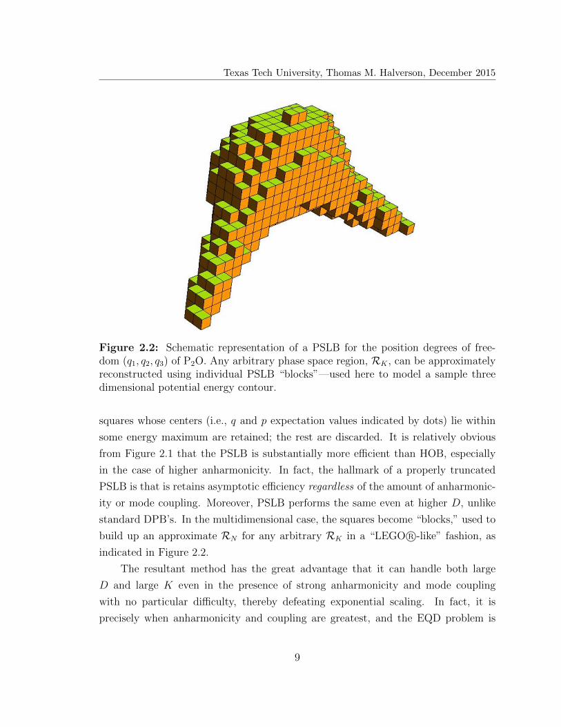
Figure 2.2: Schematic representation of a PSLB for the position degrees of free-dom (q1, q2, q3) of P2O. Any arbitrary phase space region, RK , can be approximatelyreconstructed using individual PSLB “blocks”—used here to model a sample threedimensional potential energy contour.
squares whose centers (i.e., q and p expectation values indicated by dots) lie within
some energy maximum are retained; the rest are discarded. It is relatively obvious
from Figure 2.1 that the PSLB is substantially more efficient than HOB, especially
in the case of higher anharmonicity. In fact, the hallmark of a properly truncated
PSLB is that is retains asymptotic efficiency regardless of the amount of anharmonic-
ity or mode coupling. Moreover, PSLB performs the same even at higher D, unlike
standard DPB’s. In the multidimensional case, the squares become “blocks,” used to
build up an approximate RN for any arbitrary RK in a “LEGO R©-like” fashion, as
indicated in Figure 2.2.
The resultant method has the great advantage that it can handle both large
D and large K even in the presence of strong anharmonicity and mode coupling
with no particular difficulty, thereby defeating exponential scaling. In fact, it is
precisely when anharmonicity and coupling are greatest, and the EQD problem is
9

Texas Tech University, Thomas M. Halverson, December 2015
the most challenging, that PSLB is most effective. This is because individual blocks
becomes vanishingly small compared to RK . On the other hand, at low energies, the
unphysical “blockiness” of RN [Figure 2.1(b)] leads to some numerical inefficiency. It
is this dichotomy—i.e., HOB works well at low energy, and PSLB works well at high
energy—for which the most recent version of SwitchBLADE was developed.
2.3 The Symmetrized Gaussian Basis Set
So far we have only spoken of PSLB’s in vague terms. In general, any set of
basis functions that is localized in phase space constitutes a PSLB and is amenable
to PST. However, not all PSLB’s display the properties necessary for the defeat of
exponential scaling, despite their usefulness in fields like signals processing.39–42 This
is the exact problem that was encountered in the original work of D&H, where they
attempted to use the most obvious choice of critically dense (∆2 = 2π or one function
per Planck cell) phase space Gaussian functions,
G(1)mn(q, p) =
1
πe−(q−m
√2π)2−(p−n
√2π)2
(2.10)
where m and n are the Gaussian center indices, and the “(1)” superscript denotes
the critically dense lattice spacing. If we transform Eq. (2.10) from phase space to
position space via an inverse Wigner transform,33 we get a basis set that is both
complete and linearly independent,
〈q|gmn〉 = g(1)mn(q) =
1
π1/4Exp[−1
2(q −m
√2π)2 + i(n
√2πq −mnπ)]. (2.11)
This basis set (critically dense Gaussians on a Von Neumann lattice43), however, ul-
timately fails to increase basis efficiency via PST, but for reasons that would not be
understood for many years. In work done in the early 2000’s, Poirier and coworkers
were able to show that despite the individual functions in Eq. (2.11) being as local-
ized in phase space as possible, they do not display the necessary “collective” locality
necessary for proper PST.19–22 Collective locality requires both that the individual
functions be well localized, which is the case for Eq. (2.11), and that they be orthogo-
nal, which is definitely not the case for Eq. (2.11). In fact what Poirier and coworkers
found after attempted to create a new, orthogonal basis set via a Lowdin canonical
10

Texas Tech University, Thomas M. Halverson, December 2015
orthogonalization44,45 of Eq. (2.11),
|φm′n′〉 =∑m,n
[S−1/2]m′n′mn|gmn〉, (2.12)
where S = 〈gm′n′ |gmn〉, is that the new basis set (a weylet basis) does not decay
exponentially outside the quasiclassical region—i.e., too much of the basis function’s
phase space density is far away from the center, making PST ineffective. It turns out
that this is true for any critically dense phase space localized basis set—they cannot
simultaneously be well localized and orthogonal.46,47
To remedy this problem, consider a move from the critically dense lattice (∆2 =
2π) to a half dense lattice (∆2 = 4π or one function for every two Planck cells).
At half density, the set of Gaussians do indeed exhibit collective locality; canoni-
cal orthogonalization now leads to orthogonal wavelets with exponential decay. This
change is due to the greatly decreased overlap between neighboring Gaussian func-
tions. However, by obviating collective non-locality, we have introduced a new prob-
lem: incompleteness. We no longer have enough functions to span the Hilbert space,
which means that the half-dense grid does not constitute a viable basis choice either,
despite exhibiting the type of locality required.
On the other hand, the doubly dense grid (∆2 = π or two functions per Planck
cell) has the opposite problem, in that we now have too many functions than are
needed, resulting in overcompleteness. Moreover, one could conclude that because of
the increased lattice spacing, double dense Gaussians would have even more overlap
than at critical density, but this is not the case. To explain this we exploit a reciprocal
lattice property, which establishes a kind of equivalence between a grid at density δ
and the reciprocal grid at density 1/δ. This relationship can be seen in the case of
the full set of coherent state basis functions, for which δ → ∞ and 1/δ → 0. In
this case, the reciprocal lattice Gaussians approach mutual orthogonality. This fact
is very closely related to the well-known resolution of the identity property, satisfied
by the full coherent state basis, despite its overcompleteness.48,49 This relationship
shows that overlap is maximal at critical density, and only reduces when moving
to either sub- or super-critical density—i.e., it proves that the because the former
satisfies collective locality so does the latter.20 By applying the new, super-critical
11

Texas Tech University, Thomas M. Halverson, December 2015
density to Eq. (2.11) we arrive at,
〈q|gmn〉 = g(2)mn(q) =
1
π1/4Exp[−1
2(q −m
√π)2 + i(n
√πq − mnπ
2)]. (2.13)
If this new basis set is then orthogonalized via Eq. (2.12), the new functions decay
exponentially, or better, outside the quasiclassical region.20 However, utilizing the
entire set of doubly dense Gaussians leads to numerically instability due to linear
dependencies, which, in turn, leads to exponential scaling. This unsuccessful strategy
was also tried by D&H.18
To address this final difficulty—i.e. linear dependence—momentum symmetriza-
tion is exploited. We create a new, linearly independent set of basis functions by tak-
ing a specific superposition of each ±n pair of doubly dense Gaussians.19–21,50 The re-
sultant SGB forms a complete, linearly-independent set with collective localization—
i.e., the desired goal. Moreover, the linear combination of two imaginary exponentials
yields a real valued function,
φmn(q) =1√2
[e−iπ2
(nm+n+1)g(2)mn(q) + ei
π2
(nm+n+1)g(2)m(−n)(q)]
= (4/π)1/4e−12
(q−m√π)2
sin[n√πq − nπ
2(2m+ 1)], (2.14)
which, in the end, is more numerically convenient. Because of momentum symmetry,
n is restricted to positive half-integer values, since the n = 0 states have no symmetric
counterpart. However, m has no such restriction—i.e., m = {..., ε − 1, ε, ε + 1, ...},for an arbitrary shift parameter, ε. SwitchBLADE is only currently setup for ε = 0
or ε = 1/2. In general, the choice of ε is arbitrary, having limited effect on perfor-
mance,21,51 and the restrictions only exist for pragmatic reasons (See Chapter 3). In
any event, the collective locality of the SGB can now be utilized with a proper PST
scheme,
H(m1
√π, n1
√π, ...,mD
√π, nD
√π) ≤ Emax, (2.15)
where H is the classical Hamiltonian and Emax is a truncation parameter, to defeat
exponential scaling as per the discussion in Section 2.2.
12

Texas Tech University, Thomas M. Halverson, December 2015
It should be noted that we could use Eq. (2.12) on the SGB. In fact, this is
what Poirier and Coworkers did, creating the first basis to formally defeat exponen-
tial scaling—momentum symmetrized weylets.20–22 However, the marginal gains in
performance achieved by implementing orthogonality are somewhat overshadowed by
the numerical inconvenience (see Chapter 4). In using SGB’s over weylets, we need
to take into account that the non-orthogonality of the representational basis implies
the use of the generalized matrix eigenvalue problem,
H|Ψ〉 = λ S|Ψ〉. (2.16)
This, in turn, requires explicit calculation and storage of the both the Hamiltonian
matrix, H, and the overlap matrix, S, which does increase the computational storage
needs.
For Hamiltonians of the form in Eq. (2.2) it is possible to obtain analytic matrix
elements. Since the FFP is a polynomial of order four in the normal mode coordinates,
we require equations for the p2 operator and qn operators where n = {0, 1, 2, 3, 4}.For simplicity, we introduce the following notational conventions:
m∆ = (m−m′) ; m+ = (m+m′)
n∆ = (n− n′) ; n+ = (n+ n′)
ζ(m,n,m′, n′) =π
2(m∆n+ + n∆). (2.17)
In terms of these quantities, the explicit matrix elements can be written as,
〈φm′n′ |p2|φmn〉 = p2m′n′mn =
π
2(p2(m,n,m′, n′)− p2(m,n,m′,−n′))
p2(m,n,m′, n′) = e−π4
(m2∆+n2
∆)[1
2(n2
+ −m2∆ +
2
π) cos(ζ)
−m∆n+ sin(ζ)] (2.18)
〈φm′n′ |q0|φmn〉 = sm′n′mn = s(m,n,m′, n′)− s(m,n,m′,−n′)
s(m,n,m′, n′) = e−π4
(m2∆+n2
∆) cos(ζ) (2.19)
13
Texas Tech University, Thomas M. Halverson, December 2015
〈φm′n′|q2|φmn〉 = qm′n′mn =
√π
2(q1(m,n,m′, n′)− q1(m,n,m′,−n′))
q1(m,n,m′, n′) = e−π4
(m2∆+n2
∆)[m+ cos(ζ)− n∆ sin(ζ)] (2.20)
〈φm′n′|q2|φmn〉 = q2m′n′mn =
π
2(q2(m,n,m′, n′)− q2(m,n,m′,−n′))
q2(m,n,m′, n′) = e−π4
(m2∆+n2
∆)[1
2(m2
+ − n2∆ +
2
π) cos(ζ)
+ n∆m+ sin(ζ)] (2.21)
〈φm′n′|q3|φmn〉 = q3m′n′mn =
√π
8(q3(m,n,m′, n′)− q3(m,n,m′,−n′))
q3(m,n,m′, n′) = e−π4
(m2∆+n2
∆)[(6m+ + π(m3+ − 3m+n
2∆)) cos(ζ)
+ (6n∆ + π(3m2+n∆ − n3
∆)) sin(ζ)] (2.22)
〈φm′n′|q4|φmn〉 = q4m′n′mn =
π
16(q4(m,n,m′, n′)− q4(m,n,m′,−n′))
q4(m,n,m′, n′) = e−π4
(m2∆+n2
∆)[(12m2+ − 12n2
∆ + π(m4+ − 6m2
+n2∆ + n4
∆)
+12
π) cos(ζ)− (24m+n∆ + π(4m3
+n∆ − 4m+n3∆))
× sin(ζ)]. (2.23)
2.4 The Harmonic Oscillator Basis Set (revisited)
Much work has gone into creating a new methodology that formally defeats
exponential scaling (SGB’s). It is the result of a rigorous analysis using phase space.
However, the use of the PSP does not stop there. We now revisit the issue that was
alluded to in Section 2.1 involving the energy-based truncation of HOB, and attempt
to utilize the PSP to explain the weaknesses (and strengths) of HOB. Moreover, the
ultimate goal is to utilize a phase space based analysis to design a better truncation
scheme for HOB, in a hope that we can improve its performance.
The tools utilized are the same as before, Eq. (2.7) and Eq. (2.8) under the
assumption that our basis is of the form as Eq. (2.4), but instead of having ar-
bitrary basis functions, we have HOB functions, |n1, n2, ..., nD〉, where nk has the
14
Texas Tech University, Thomas M. Halverson, December 2015
physical meaning of being the nth excitation of the kth mode. As has been discussed
throughout, to mitigate the curse of dimensionality, we must employ some correlated,
non-DPB truncation criterion. For HOB’s we choose,
D∑j=1
αjnj ≤ Emax, (2.24)
which restricts the energy configuration, {n1, n2, ..., nD}, of each HOB function such
that the weighted sum of the individual mode excitations is less than some maximum
energy. This greatly reduces N , and can also greatly improve HOB efficiency—
provided that the αj’s are chosen in a way that is tailored for the specific application.
In the past, these coefficients have been chosen in somewhat ad hoc fashion,10,11,52
with very little evidence provided for why one choice is better than another. Here,
we hope to answer the question of what αj choices are best via systematic analysis
of the possible choices. More specifically, what choices optimize a given calculation
within a given desired spectral range?
The basic idea is the same as Section 2.2 in that the K quantum states of
interest—i.e., those that lie below some energy threshold—define some well-defined
classical region of phase space.18,38 Any representational basis meant to compute all
K states must, as a necessary condition, incorporate this classical region, within
which most of the quantum probability resides. However, if higher accuracy is de-
sired, the representational basis must extend beyond the classical region, in order
to also incorporate quantum tunneling probability. Thus, whereas the classical PSP
provides an invaluable starting point, a more rigorous analysis requires a quantum
PSP treatment—specifically, the Wigner PDF.32,33,36
To help visualize the issue at hand, we utilized a slice of the Hamiltonian, similar
to what was used in Section 2.2. However, here we need to be able to observe the
effect of “correlation” between the degrees of freedom. This requires more information
than f = 2 would be able to provide. Instead, we utilize the slice of the full f = 60
Hamiltonian for C6H6, where all phase space coordinates are set to zero except j=2
(in-plane anti-symmetric stretch) and j=5 (out-of-plane anti-symmetric bend), where
15

Texas Tech University, Thomas M. Halverson, December 2015
the mode labeling is that of Wilson,53
h(2)(q2, p2, q5, p5) = 1604.0(p22 + q2
2) + 505.0(p25 + q2
5)− 137.87q32 + 7.20q4
2
+3.39q45 + 137.75q2q
25 − 26.60q2
2q25, (2.25)
in units of cm−1 (for more information about the full FFP See Chapter 8). Obviously,
there are many mode pairs that could have been chosen, but (2, 5) exhibits a moderate
or “typical” amount of anharmonicity and mode coupling for the benzene system.
We will first consider two natural choices for the αj coefficients in Eq. (2.24). For
the first choice, all modes are equally weighted, αj = 1; this is called polyad truncation
(PT). For the second choice, the coefficients are chosen to be the harmonic frequencies
of the corresponding normal modes, i.e. αj = ωj; this is called frequency truncation
(FT). Of course, these are not the only choices, but we shall find it convenient to
regard these two as the opposite ends of a spectrum of possibilities.
To begin this analysis we must first solve Eq. (2.7) to get the Wigner PDF,
ρK(q2, p2, q5, p5). Of course, calculating ρK requires computation of the eigenvectors,
which we obtained by diagonalizing the Hamiltonian matrix of Eq. (2.3) for H = h(2)
and {|Φj〉}Nj=1, using a very large HOB. Specifically, a sufficiently large N was chosen
such that K = 20 states were all converged to ∼ 10−2 cm−1 or better. The position-
space projection of this Wigner PDF can be seen in Figure 2.3(a). The choice K =
20 corresponds roughly to the dynamically relevant range for the h(2) system; from
Figure 2.3(b), the anharmonicity/coupling is readily apparent.
Next, we calculated projection operators for candidate representational HOB’s
using Eq. (2.8) for two truncation methods, PT and FT, with Emax chosen for each
such that N≈K. This is the smallest possible N value with any chance of spanning
the desired classical phase space region. From Eq. (2.4), we know that for PT, the
set of retained D=2 basis functions, |n2, n5〉, corresponds to a “symmetric triangle”
of points in (n2, n5) space, which is obviously invariant with respect to coordinate
exchange. This coordinate exchange permutation symmetry is evident in the corre-
sponding ρN Wigner PDF, as can be seen in Figure 2.4. Indeed, from the figure, it
is clear that ρN exhibits not only exchange symmetry but also pure rotational sym-
metry, with respect to the q2 and q5 coordinates. In any event, nmax is clearly the
same for both coordinates. All of this is in stark contrast to the ρK distribution of
16

Texas Tech University, Thomas M. Halverson, December 2015
Figure 2.3: Position space projection of the ρK Wigner PDF for the density operatorof the K = 20 lowest lying eigenstates of the D = 2 h(2) Hamiltonian of Section 2.4:(a) 3D plot; (b) contour plot.
Figure 2.3, which exhibits an oblong shape that is much more extended along q5 than
q2, owing to the smaller ω5 < ω2 frequency. In any event, for N≈K, the desired ρK
and representational ρN PDF’s are not even qualitatively close to each other, and so
the PT basis yields very low efficiency.
On the other hand, the classical PSP predicts that FT should do a much better
job at capturing the desired classical phase space region, when N ≈ K. This is
because Eq. (2.24) effectively becomes the true classical Hamiltonian, apart from
anharmonicity/coupling. More specifically, the FT choice provides a higher nmax for
q5 than for q2 because of the smaller ω5 value—exactly as it should. Indeed, as
indicated in Figure 2.5, the resultant FT ρN Wigner PDF is an oval, elongated along
q5, that closely resembles the true ρK—at least within the classical region. It is this
similarity in shape that results in much higher basis efficiency for FT than for PT, in
cases when N≈K. In any event, this result should not be too surprising, given that
PT uses no system-specific information at all to determine its αj’s, whereas FT at
least incorporates harmonic frequencies. However, the FT customization is relatively
limited, as it does not take into account any of the mode coupling and anharmonicity,
which are also evident in Figure 2.3(b). Specifically, these manifest as distortions from
17
Texas Tech University, Thomas M. Halverson, December 2015
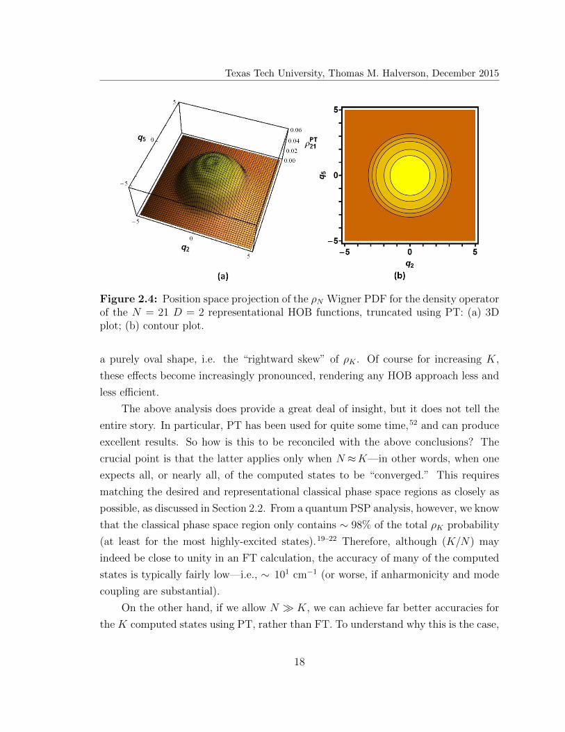
Figure 2.4: Position space projection of the ρN Wigner PDF for the density operatorof the N = 21 D = 2 representational HOB functions, truncated using PT: (a) 3Dplot; (b) contour plot.
a purely oval shape, i.e. the “rightward skew” of ρK . Of course for increasing K,
these effects become increasingly pronounced, rendering any HOB approach less and
less efficient.
The above analysis does provide a great deal of insight, but it does not tell the
entire story. In particular, PT has been used for quite some time,52 and can produce
excellent results. So how is this to be reconciled with the above conclusions? The
crucial point is that the latter applies only when N ≈K—in other words, when one
expects all, or nearly all, of the computed states to be “converged.” This requires
matching the desired and representational classical phase space regions as closely as
possible, as discussed in Section 2.2. From a quantum PSP analysis, however, we know
that the classical phase space region only contains ∼ 98% of the total ρK probability
(at least for the most highly-excited states).19–22 Therefore, although (K/N) may
indeed be close to unity in an FT calculation, the accuracy of many of the computed
states is typically fairly low—i.e., ∼ 101 cm−1 (or worse, if anharmonicity and mode
coupling are substantial).
On the other hand, if we allow N � K, we can achieve far better accuracies for
the K computed states using PT, rather than FT. To understand why this is the case,
18

Texas Tech University, Thomas M. Halverson, December 2015
Figure 2.5: Position space projection of the ρN Wigner PDF for the density operatorof the N = 20 D = 2 representational HOB functions, truncated using FT: (a) 3Dplot; (b) contour plot.
we must apply the quantum PSP to examine the long-range tunneling behavior of
the requisite PDF’s—since high convergence requires the inclusion of deep tunneling
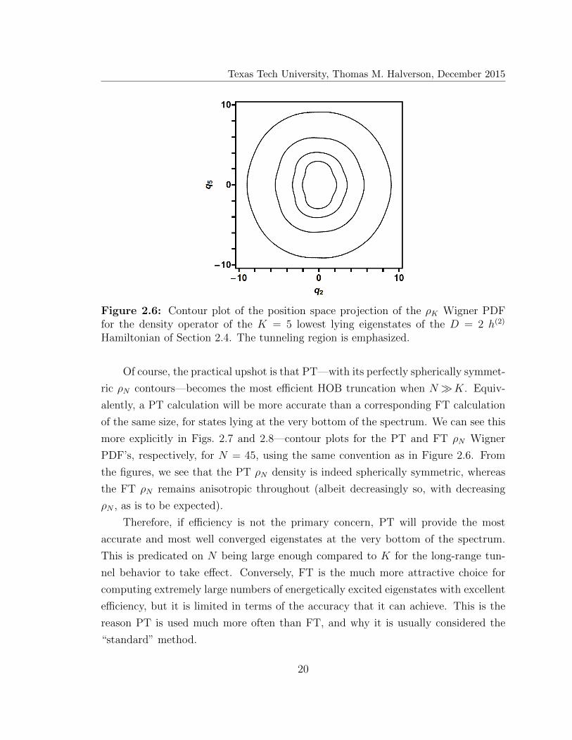
probabilities, from well beyond the classical phase space region. In Figure 2.6 we
present the long range tunneling of the ρK Wigner PDF for K = 5, for h(2). Here,
in order to properly reflect the higher desired target accuracy, the calculation was
converged to ∼10−4 cm−1 or better for each of the K=5 eigenstates.
In Figure 2.6, the innermost contour corresponds roughly to the classical phase
space region, whereas the larger concentric contours correspond to the rapidly de-
caying values of ρK in the quantum tunneling region, down to well below numerical
precision. Any representational basis that captures the region defined by the largest
contour should therefore suffice to compute the lowest K = 5 quantum states “ex-
actly”. The main conclusion to draw from the figure is that for higher accuracies, the
contours become increasingly circular, not elliptical. The reason for this is simply un-
derstood in terms of the long-range decay of the HOB functions themselves—which
scales as the same Gaussian for all normal modes, regardless of excitation, nj, or
frequency, ωj.
19
Texas Tech University, Thomas M. Halverson, December 2015
Figure 2.6: Contour plot of the position space projection of the ρK Wigner PDFfor the density operator of the K = 5 lowest lying eigenstates of the D = 2 h(2)
Hamiltonian of Section 2.4. The tunneling region is emphasized.
Of course, the practical upshot is that PT—with its perfectly spherically symmet-
ric ρN contours—becomes the most efficient HOB truncation when N�K. Equiv-
alently, a PT calculation will be more accurate than a corresponding FT calculation
of the same size, for states lying at the very bottom of the spectrum. We can see this
more explicitly in Figs. 2.7 and 2.8—contour plots for the PT and FT ρN Wigner
PDF’s, respectively, for N = 45, using the same convention as in Figure 2.6. From
the figures, we see that the PT ρN density is indeed spherically symmetric, whereas
the FT ρN remains anisotropic throughout (albeit decreasingly so, with decreasing
ρN , as is to be expected).
Therefore, if efficiency is not the primary concern, PT will provide the most
accurate and most well converged eigenstates at the very bottom of the spectrum.
This is predicated on N being large enough compared to K for the long-range tun-
nel behavior to take effect. Conversely, FT is the much more attractive choice for
computing extremely large numbers of energetically excited eigenstates with excellent
efficiency, but it is limited in terms of the accuracy that it can achieve. This is the
reason PT is used much more often than FT, and why it is usually considered the
“standard” method.
20
Texas Tech University, Thomas M. Halverson, December 2015
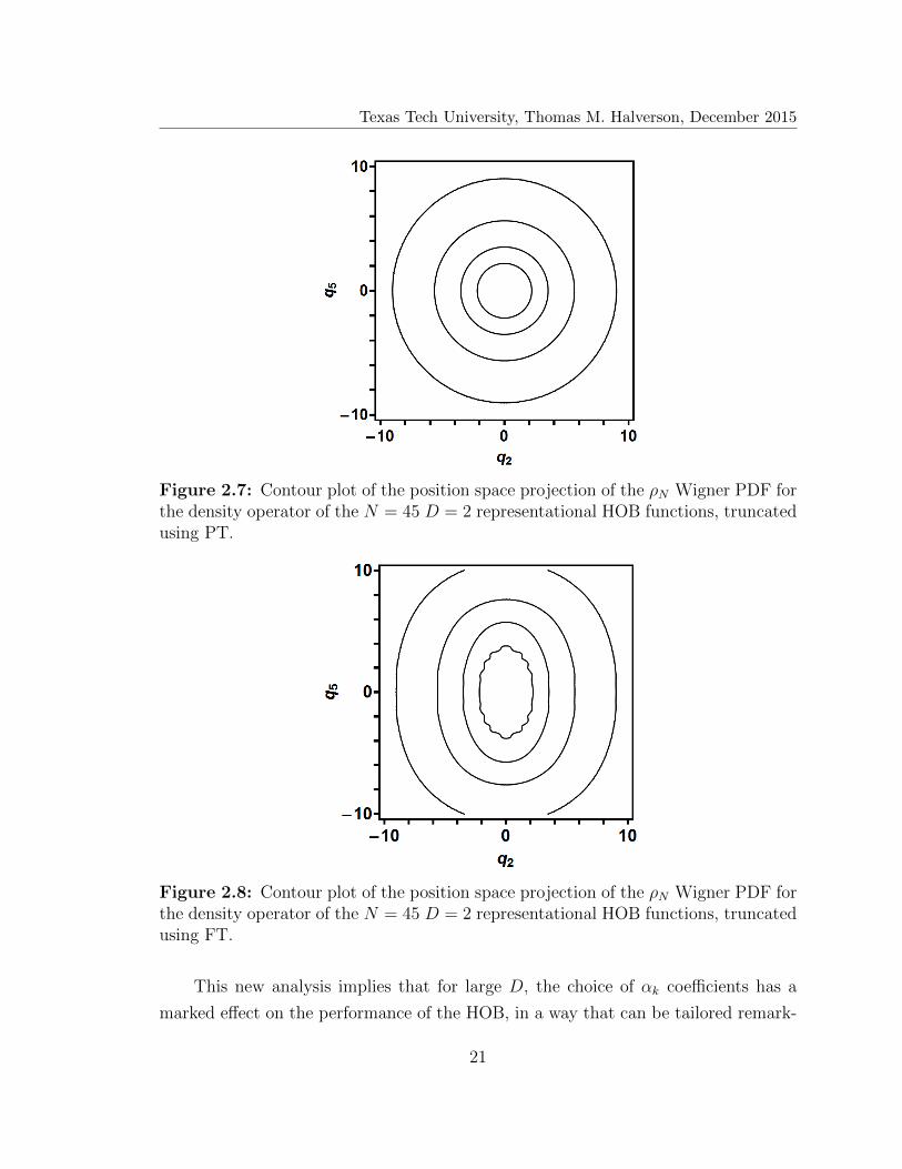
Figure 2.7: Contour plot of the position space projection of the ρN Wigner PDF forthe density operator of the N = 45 D = 2 representational HOB functions, truncatedusing PT.
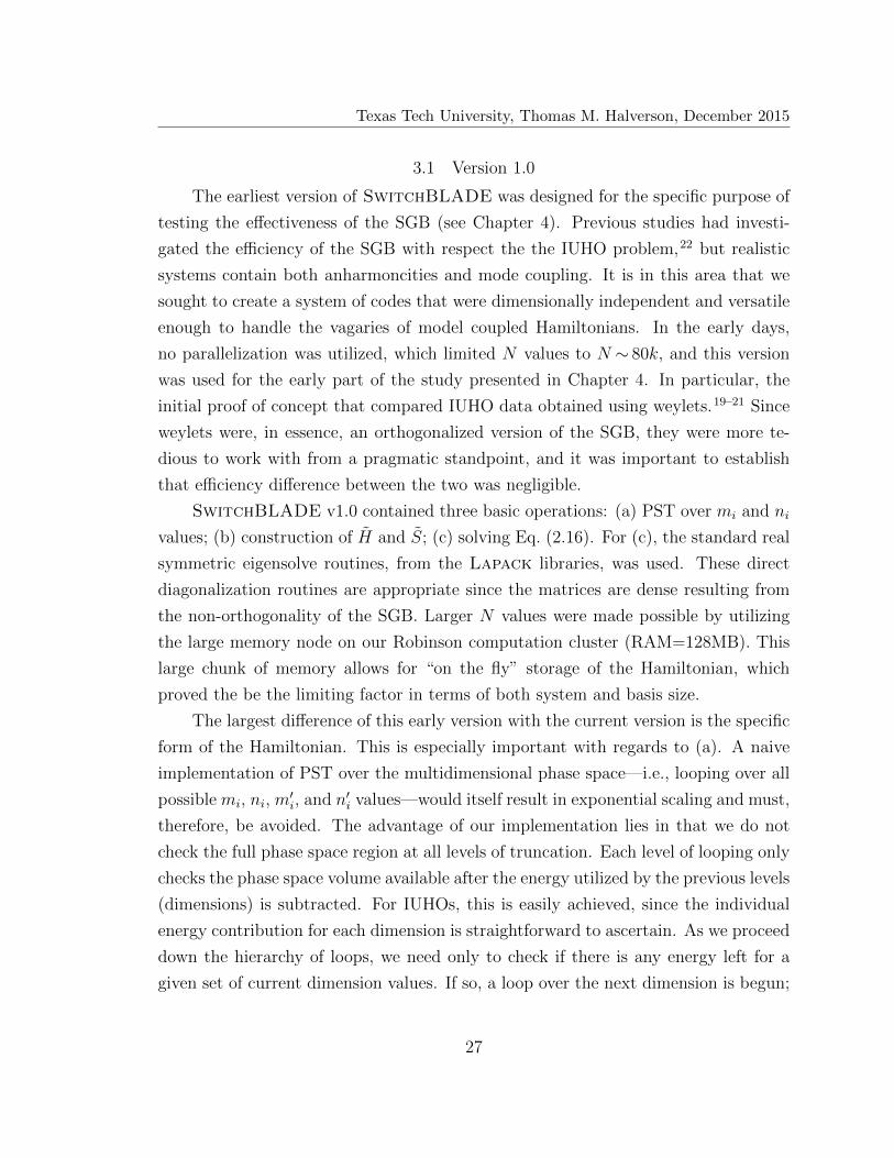
Figure 2.8: Contour plot of the position space projection of the ρN Wigner PDF forthe density operator of the N = 45 D = 2 representational HOB functions, truncatedusing FT.
This new analysis implies that for large D, the choice of αk coefficients has a
marked effect on the performance of the HOB, in a way that can be tailored remark-
21

Texas Tech University, Thomas M. Halverson, December 2015
ably well for specific spectral domains. The closer the αk are to the ωk, the higher
we can go in the spectrum and still obtain reasonably well converged results. As all
of the αk’s approach the same value, however, we obtain very high accuracy in the
lowest part of the spectrum, but quickly lose even qualitatively correct behavior with
increasing excitation energy (with errors typically growing nearly exponentially).
The above facts suggests that a “compromise” between FT and PT might work
best in intermediate energy domains—particularly in cases where D is large, and/or
when there is a substantial spread in ωk values. One way to explore this idea is to
replace Eq. (2.24) withD∑j=1
(ωj)µ nj ≤ Emax, (2.26)
where 0 ≤ µ ≤ 1. This allows us to work with the single truncation parameter, µ,
rather than with D separate parameters.
By comparing Eqs. (2.24) and (2.26), it becomes clear that µ = 0.0 corresponds
to PT, whereas µ = 1.0 corresponds to FT. This “µ-truncation” gives us great control
over N , which is not the case for traditional µ = 0.0. The extremely high symmetry
of true PT results in very large sudden jumps in N as Emax is increased. This makes
it very difficult to “tune” the PT basis size—a property which is desirable, among
other reasons, because it enables accurate convergence testing. At low D this is not
a problem, again showcasing why it has always been considered the standard. For
example, Eq. (2.26) with the parameters, D = 3, µ = 0.0, and Emax = 10, would
yield 3N0.010.0 = 286, where we utilize the notation, DNµ
Emax. If we increase Emax by a
factor of 2, we get 3N0.020.0 = 1771, which is only a modest increase. However, if we
increase to D = 9, a 2-fold increase in Emax yields a much more substantial jump,9N0.0
5 = 2002 to 9N0.010 = 92378. When we move to very large D, e.g. D = 30, this
discreteness becomes so large that systematic basis set convergence testing is nigh
impossible—i.e., 30N0.05 = 324, 632 jumps suddenly to 30N0.0
6 = 1, 947, 792 with no
possible values in between. As a pragmatic measure, we don’t actually work with
µ = 0.0 when D is large, but rather, we use the very small value, µ = 0.1, instead.
This provides much finer gradations in N , while still providing a truncated basis that
is very similar to µ = 0.0. For instance, if we take the ω’s in Eq. (2.26) to be those of
22

Texas Tech University, Thomas M. Halverson, December 2015
C6H6, we get 30N0.1180.0 = 315, 061, but unlike µ = 0.0, a small increase in Emax yields
a marginal increase in N , e.g. 30N0.1185.0 = 414, 212.
Beyond facilitating more logical, systematic convergence testing, the use of Eq. (2.26)
allows us to compare results from different µ values, since we can ensure the similarity
of N values from one truncation method to the next. It is worth noting again that
all HOB representations, as implemented in SwitchBLADE, are rigorously varia-
tional—meaning that all computed energy levels converge from above to the exact
results, as Emax is increased. Of course, for comparable N values, a lower µ calcula-
tion should yield more accurate—and therefore lower—energy levels, Ek, in the lower
part of the spectrum, whereas a higher µ calculation will yield lower/more accurate
eigenvalues further up in the spectrum. In any event, for a given eigenstate, k, the
lowest energy level, Eµk , computed across different µ values, is the most accurate.
This suggests a natural way to combine the different truncation schemes together,
to create a “best of all worlds” dataset: one simply compares a sorted list of computed
energy levels for each separate µ calculation; for each eigenstate k, one then selects the
lowest of the Eµk values as the most accurate computed energy level for that state. We
call this the hybrid truncation (HT) dataset. In principle, HT does not even require
that the respective N ’s for each calculation be comparable to each other. However,
if one wishes to quantify convergence for the HT dataset in a consistent manner then
the various DNµEmax
values for the different µ calculations should be similar.
Because it incorporates different types of truncation that are optimal for different
energy regimes, the HT dataset will be more accurate overall than any other specific
µ value, throughout the entire spectrum. We could, in essence, combine as many
different µ calculations as we like, but for simplicity sake, here we combine calculations
from µ = 0.1 (or µ = 0.0 when possible) with µ = 1.0, in addition to µ = 0.5, lying
“halfway” between µ = 0.1 and µ = 1.0. Generally speaking, one expects the lowest-
lying states to come from µ = 0.1, the intermediate states from µ = 0.5, and the
high-lying states from µ = 1.0. However, there are some exceptions to this basic
pattern—such as a partially excited overtone for a low-frequency mode. µ = 0.1 does
not do well for such states, even if Ek is rather low, because it treats all modes equally.
The above analysis is formally rigorous where HT energy levels are concerned;
however, there may in principle be some subtleties with regard to the corresponding
23

Texas Tech University, Thomas M. Halverson, December 2015
energy eigenvectors. One question that does arise is the orthogonality of the eigen-
states between the methods used in the hybridization process. Since we are cherry
picking states from each set of calculations simply based on lowest lying eigenvalue,
we have no assurances that the eigenvectors retain their orthogonality (or even their
linear independence). A full analysis of this problem is beyond the scope of what
is presented herein. However, for the above D = 2 example the condition number
of the overlap matrix for the hybrid basis set is within ∼ 3% of the identity even
if the N is small (∼ 30) and the states are not very well converged. This regime is
the “worst case scenario” since the convergence is on the order of the level spacing.
However, this will give a better indication of what the overlap matrix would look like
at higher D—i.e., when there exists a regime in which any method is equally as likely
to be chosen by the hybridization process. At very high levels of convergence, the
bifurcation between methods is very clearly defined and the condition number of the
overlap is within ∼ 0.1% of the identity, but for large D this level of convergence is
difficult to achieve.
Lastly, in the same vein as the SGB in Section 2.3, we can compute analytic
matrix elements for the operators present in Eq. (2.2)—i.e., the p2 operator and the
qn operators where n = {1, 2, 3, 4} (note that n = 0 is ignored since HOB functions
are orthogonal). This can be accomplished by utilizing the standard ladder operators,
yielding,
〈m|p2|n〉 = p2m,n =
1
2[(2n+ 1) δm,n −
√(n+ 1)(n+ 2) δm,n+2
−√n(n− 1) δm,n−2], (2.27)
〈m|q|n〉 = qmn =
√1
2(√n+ 1 δm,n+1 +
√n δm,n−1), (2.28)
〈m|q2|n〉 = q2mn =
1
2[√
(n+ 1)(n+ 2) δm,n+2 +√n(n− 1) δm,n−2
+ (2n+ 1) δm,n], (2.29)
24

Texas Tech University, Thomas M. Halverson, December 2015
〈m|q3|n〉 = q3mn =
(1
2
)2/3
[√
(n+ 1)(n+ 2)(n+ 3) δm,n+3
+√n(n− 1)(n− 2) δm,n−3 + (3n+ 3)
√n+ 1 δm,n+1
+ 3n√n δm,n−1], (2.30)
〈m|q4|n〉 = q4mn =
(1
2
)[√
(n+ 1)(n+ 2)(n+ 3)(n+ 4) δm,n+4
+√n(n+ 1)(n+ 2)(n+ 3) δm,n−4
+ (4n+ 6)√
(n+ 1)(n+ 1) δm,n+2
+ (4n− 2)√n(n− 1) δm,n−2
+ +(6n2 + 6n+ 3) δm,n], (2.31)
where δm,n is the Kronecker delta function.
25

Texas Tech University, Thomas M. Halverson, December 2015
CHAPTER 3
SWITCHBLADE AND COMPUTATIONAL SCALING
The underlying goal throughout this project has always been the creation of
standalone, black-box code for distribution to the computational chemistry commu-
nity, under the guise that the code should not only be versatile and efficient, but
also easy to use. From a computational standpoint, a general EQD problem can be
broken down into three steps: a) Choosing a representational basis set; b) Truncating
the set of basis functions given a specific scheme (See. Chapter 2); c) Creation and
diagonalization of the Hamiltonian matrix. To this end, we have developed Switch-
BLADE, which in its most current implementation, utilizes Fortran 90 and MPI
combined with two general basis sets, HOB and SGB, and their respective truncation
schemes. Over the years many changes have been implemented into SwitchBLADE,
which will be discussed below, but none of the “bells and whistles” change the overall
concept. The whole system is predicated on utilizing well known, direct diagonaliza-
tion libraries (e.g. Lapack and Scalapack). Because SwitchBLADE uses these
libraries, which are widely distributed, it can utilized by many different users, regard-
less of access to cutting edge computational platforms. However, SwitchBLADE is
designed to take advantage of newer, state-of-the-art systems, when available—i.e.,
the scalability of the newest versions is quite good, with the diagonalization step
being the bottleneck,54 allowing for parallelization up ∼103 computational cores.
Beyond the obvious, what makes the SwitchBLADE system truly unique
among the pantheon of computational software is the user functionality. From day
one, SwitchBLADE was designed with ease of use in mind. All the user must
provide is a properly formatted FFP input file and the code will compute vibra-
tional eigenstates regardless of D!. This is in stark contrast to most EQD software
packages, which are either limited to a specific D (or small set of D’s)12 or require
massive customization to the source code for each individual system of interest.15
Despite all the work that has been done over the past years, SwitchBLADE is still
in its fledgling stage, and much work still needs to be done before it is ready for large
scale distribution. However, the foundation on which is was built—i.e., PSP based
basis truncation—provides very solid footing for future version.
26
Texas Tech University, Thomas M. Halverson, December 2015
3.1 Version 1.0
The earliest version of SwitchBLADE was designed for the specific purpose of
testing the effectiveness of the SGB (see Chapter 4). Previous studies had investi-
gated the efficiency of the SGB with respect the the IUHO problem,22 but realistic
systems contain both anharmoncities and mode coupling. It is in this area that we
sought to create a system of codes that were dimensionally independent and versatile
enough to handle the vagaries of model coupled Hamiltonians. In the early days,
no parallelization was utilized, which limited N values to N ∼ 80k, and this version
was used for the early part of the study presented in Chapter 4. In particular, the
initial proof of concept that compared IUHO data obtained using weylets.19–21 Since
weylets were, in essence, an orthogonalized version of the SGB, they were more te-
dious to work with from a pragmatic standpoint, and it was important to establish
that efficiency difference between the two was negligible.
SwitchBLADE v1.0 contained three basic operations: (a) PST over mi and ni
values; (b) construction of H and S; (c) solving Eq. (2.16). For (c), the standard real
symmetric eigensolve routines, from the Lapack libraries, was used. These direct
diagonalization routines are appropriate since the matrices are dense resulting from
the non-orthogonality of the SGB. Larger N values were made possible by utilizing
the large memory node on our Robinson computation cluster (RAM=128MB). This
large chunk of memory allows for “on the fly” storage of the Hamiltonian, which
proved the be the limiting factor in terms of both system and basis size.
The largest difference of this early version with the current version is the specific
form of the Hamiltonian. This is especially important with regards to (a). A naive
implementation of PST over the multidimensional phase space—i.e., looping over all
possible mi, ni, m′i, and n′i values—would itself result in exponential scaling and must,
therefore, be avoided. The advantage of our implementation lies in that we do not
check the full phase space region at all levels of truncation. Each level of looping only
checks the phase space volume available after the energy utilized by the previous levels
(dimensions) is subtracted. For IUHOs, this is easily achieved, since the individual
energy contribution for each dimension is straightforward to ascertain. As we proceed
down the hierarchy of loops, we need only to check if there is any energy left for a
given set of current dimension values. If so, a loop over the next dimension is begun;
27
Texas Tech University, Thomas M. Halverson, December 2015
if not, execution passes back to the higher loops. In this manner, a “pruned tree” of
loops is performed, which avoids exponential scaling. The CPU time needed for PST
is thus decreased to a matter of seconds, even for larger D values.
It is the separability of the IUHO potential, and the fact each individual contri-
bution to H is positive, that guarantees that as we proceed down the loop tree, the
remaining energy contribution decreases. In the general CAHO case, negative cou-
pling and/or anharmonicity contributions, arising from odd powers of q or negative
coefficients (both of which are physically realistic), will result in the above algorithm
missing relevant areas of phase space—and therefore, not identifying the correct PST
basis. To obviate this difficulty, for the moment we consider only positive anharmonic-
ity and coupling constants, and set all odd powers of qi to zero. This ensures that
the second-order separable IUHO potential is lower in energy than the full CAHO
potential, which allows us to utilize the same truncation algorithm for both. This
is, of course, an issue that needs to be addressed if we wish to study more general
systems.
For D ≤ 4, the N values are so small that the matrix diagonalization (which
scales as N3) requires significantly less CPU time than matrix construction (which
scales as N2 or faster). As a result, the total CPU times for the SGB calculations
exhibit a less marked D dependence than might be expected. Specifically, the time
needed to compute an individual set of eigenvalues forD = 2 was less than one minute,
for D = 3 it was around one minute, and for D = 4 it was around five minutes. In
contrast, the CPU time required for PertT calculations—even though this calculation
is only approximate—increased very dramatically with D. The D = 2 calculation
required only 30 seconds, but D = 3 required over nine minutes, and D = 4 over 150
minutes.
This early study proved that at the very least, the PST SGB approach, utiliz-
ing direct diagonlization, has promise. However, two major obstacles needed to be
overcome—a more generalized version of H and computational paralellization. These
two problems turned out to be highly non-trivial, especially in the context of ease of
use and dimensional independence.
28

Texas Tech University, Thomas M. Halverson, December 2015
3.2 Version 2.0
To make SwitchBLADE more robust we first tackled the problem of the gener-
alizing the Hamiltonian to include odd powers of q and negative coupling coefficients.
The major hindrance here manifested itself in the PST algorithm. As discussed
above a naıve implementation of a full 2D phase space search reintroduces expo-
nential scaling, which has been painstakingly avoid up to now. To circumvent this
issue we utilized effective, D=1, potentials created by fixing a single coordinate and
minimizing with respect to the rest. Beyond the pragmatic application to the com-
putational algorithms, this process also proved quite useful in evaluating the quality
of a given FFP. It provided great insight into the maximum coordinate ranges ap-
plicable to the given FFP, provided information about maximum energy ranges and
any psuedo-dissociation thresholds, and also illuminated potential issues (see Chap-
ter 6 and 7). The effective potentials were computed using the CG-plus library of
conjugate gradient minimization routines.55 Given the basic PST criterion as out-
lined in Section 2.3, we discard basis functions localized around phase space points
(q1, p1, ..., qD, pD), except when
Emax ≥ H(q1, p1, ..., qD, pD). (3.1)
Instead of doing this directly for all levels of the search, correlations introduced by
the FFP are accounted for via minimization of the FFP with respect to all degrees
of freedom but the one of interest—the same strategy used in the highly successful
“phase space optimized DVR” technique.29–31
The resultant effective potentials, V effj (qj), are used to define 1-D energies,
Ej(qj, pj) =1
2ωjp
2j + V eff
j (qj), (3.2)
associated with individual phase space coordinate pairs, (qj, pj). This allows for the
pruned tree PST strategy to be used. Like before, the q and p indices for a given
coordinate level j—i.e., mj and nj—are only allowed to range over values for which
Ej ≤ Emax − E1 − E2 − ...− Ej−1, (3.3)
29
Texas Tech University, Thomas M. Halverson, December 2015
thereby dramatically reducing the total region of phase space that must be searched
explicitly. In this manner, exponential scaling is avoided yet again, despite the use of
a general Hamiltonian.
In terms of implementation, the outermost loop (really two loops) considers each
(m1, n1) pair in the range mmin1 ≤ m1 ≤ mmax
1 ; 12≤ n1 ≤ nmax
1 , with SGB centers for
the first degree of freedom located at (q1 = m1
√π, p1 = n1
√π). All phase space points
in the above ranges are evaluated to determine whether or not E1 ≤ Emax. If so, the
next set of loops is called—over (m2, n2), and with Emax replaced with (Emax−E1). If
not, the phase space point is ignored. Subsequent loops proceed in the same fashion,
until the innermost, j = f , loop is reached—at which point Eq. (3.1) is used to effect
the final PST, instead of Eq. (3.3). Surprisingly, the creation of the D − 1 effective
potentials needed in the new pruned tree PST algorithm takes a remarkably short
amount of time, regurdless of D or even the number of parameters in the FFP. This
algorithm was tested on realistic FFP’s up to D = 30, and the computational time
only varied from seconds for small D up to a few minutes for D = 30; we do not
foresee that this step will ever require parallelization.
In reality, the algorithm as described above could be “fooled”—e.g., if the region
of phase space considered is concave, rather than convex, as in the case of double-well
tunneling. We have currently implemented a work around for this issue, discussed
below. However, the underlying assumption of SwitchBLADE up to this point
is that the system has a single well. In any event, this PST algorithm will still
work perfectly for arbitrary phase space regions, if the following two refinements are
implemented. First, within the lowest-level of the loop, the exact criterion of Eq. (3.1)
is used to select points, rather than Eq. (3.3). This ensures that only legitimate phase
space points (SGB functions) are retained. Second, to avoid the possibility (unlikely
for single-well systems) of missing legitimate points, one can simply increase Emax in
Eq. (3.3), until the resultant N no longer changes.
The second issue that must be addressed is parallelization. The original code
utilized the Lapack libraries which do not take advantage of distributed memory
architectures. This was very limiting since it imposes a strict maximum on N based
on the amount of memory available on a single node of the system. Luckily, we had
access to a computational platform that had nodes with large memory blocks, allowing
30
Texas Tech University, Thomas M. Halverson, December 2015
for somewhat larger N values to be used in our early studies, but to go beyond this a
distributed memory work around had to be implemented. This was handled by using
the Scalapack libraries, which block distribute the Hamiltonian matrix across the
process grid. Since the size of the process grid is only limited by the size of the
computational cluster, very large N values are attainable despite each computational
node only having a small amount of memory. This allowed for N∼400k values to be
used, which massively increased the D range that could be studied.
The parallelization, however, was limited to the matrix creation and diagonal-
ization steps. The PST algorithm was was not written to utilize parallel methods.
There is no technical reason why this step should not parallelize effectively, but it did
not become the computational bottleneck until we reached D = 12. For the smaller
dimensional ranges look at (up to f = 9) this step takes at most a few hours, even for
the largest Emax values considered. PST for the smallest N for the P2O calculations
required only ∼ 0.5 sec., whereas the largest N took ∼ 10 sec. In the case of CH2NH,
PST for the smallest N took ∼ 30 s, but the truncation for the largest N took ∼ 30
mins. Beyond that, the computational time became intractable (> 24 hrs.), but we
will show later that parallelization is not the solution.
This version of SwitchBLADE, which combined pruned tree PST and paral-
lelization, was used to compile the larger D and N values outlined in Chapter 4, along
with the data presented in Chapters 5 and 6. A small amount of numerical scalabil-
ity was collected, but a comprehensive scaling study was not performed (up to this
point)—simply because the bottleneck is still the diagonalization step, for which the
scaling is well understood. However, the data that was collected is presented in Ta-
ble 3.1. The times present in Table 3.1 are for the matrix creation and diagonalization
step. This step was performed using MPI and the Scalapack routine PDSYGVX,
running on the parallel clusters described in the Acknowledgements (primarily Lon-
estar). The PDSYGVX routine contains some parameters that can be adjusted to
improve performance, but a full exploration of how these affect computational time
is beyond the scope of what is presented here. We adjusted these only as needed
to ensure a computational time of less than 24 hrs. (the queue limit on Lonestar).
It should be noted that we performed calculations parallelized up to ∼ 4000 cores
with relative ease, due to both the simplicity of the code and the use of single call to
31
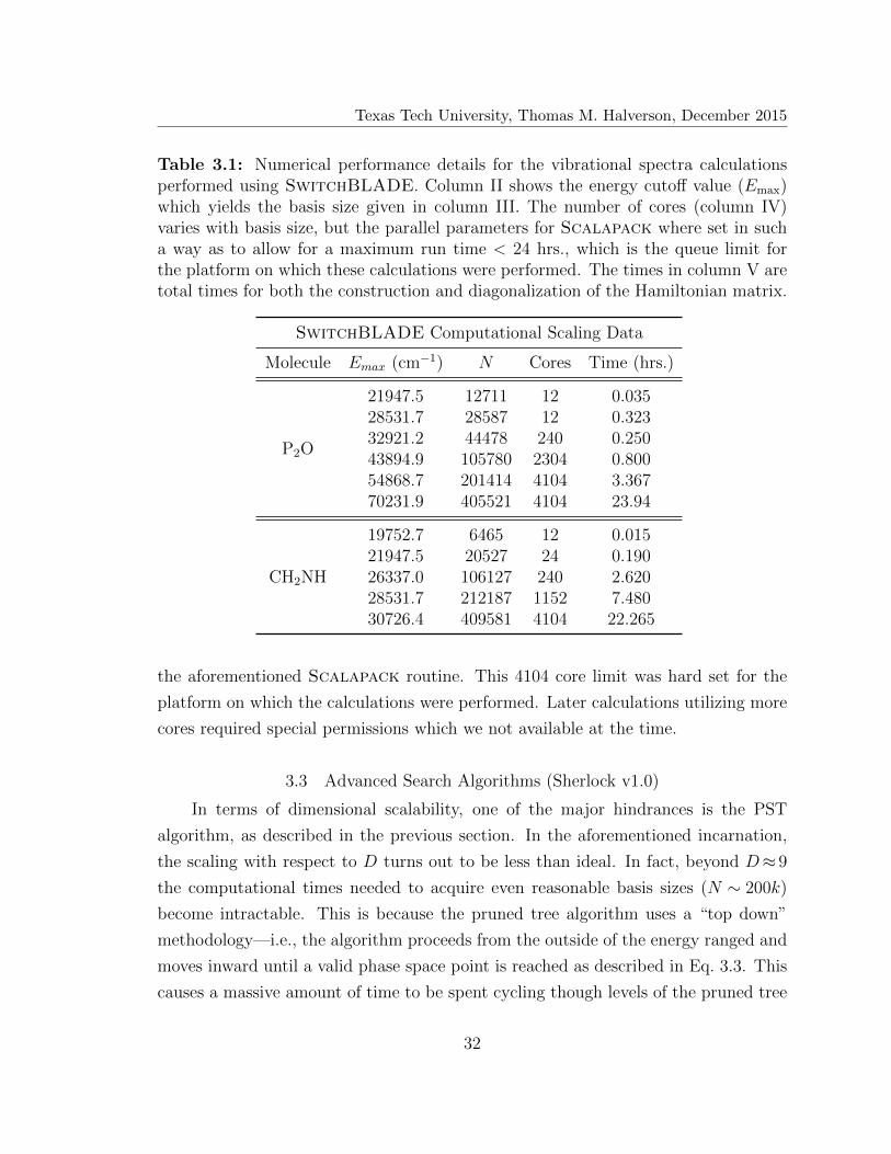
Texas Tech University, Thomas M. Halverson, December 2015
Table 3.1: Numerical performance details for the vibrational spectra calculationsperformed using SwitchBLADE. Column II shows the energy cutoff value (Emax)which yields the basis size given in column III. The number of cores (column IV)varies with basis size, but the parallel parameters for Scalapack where set in sucha way as to allow for a maximum run time < 24 hrs., which is the queue limit forthe platform on which these calculations were performed. The times in column V aretotal times for both the construction and diagonalization of the Hamiltonian matrix.
SwitchBLADE Computational Scaling Data
Molecule Emax (cm−1) N Cores Time (hrs.)
P2O
21947.5 12711 12 0.03528531.7 28587 12 0.32332921.2 44478 240 0.25043894.9 105780 2304 0.80054868.7 201414 4104 3.36770231.9 405521 4104 23.94
CH2NH
19752.7 6465 12 0.01521947.5 20527 24 0.19026337.0 106127 240 2.62028531.7 212187 1152 7.48030726.4 409581 4104 22.265
the aforementioned Scalapack routine. This 4104 core limit was hard set for the
platform on which the calculations were performed. Later calculations utilizing more
cores required special permissions which we not available at the time.
3.3 Advanced Search Algorithms (Sherlock v1.0)
In terms of dimensional scalability, one of the major hindrances is the PST
algorithm, as described in the previous section. In the aforementioned incarnation,
the scaling with respect to D turns out to be less than ideal. In fact, beyond D≈ 9
the computational times needed to acquire even reasonable basis sizes (N ∼ 200k)
become intractable. This is because the pruned tree algorithm uses a “top down”
methodology—i.e., the algorithm proceeds from the outside of the energy ranged and
moves inward until a valid phase space point is reached as described in Eq. 3.3. This
causes a massive amount of time to be spent cycling though levels of the pruned tree
32

Texas Tech University, Thomas M. Halverson, December 2015
that have no chance of leading to a valid point. Beyond the computational issues, this
method (pruned tree) has other issues, in that it is limited to cases where we have
concave phase space volumes only—i.e., single well potentials far from disassociation.
To handle more general molecular systems this issue must also be addressed directly.
What we created was a “bottom up” algorithm—Sherlock. This algorithm
utilizes psuedo-recursion to find all points within a closed surface starting from some
interior point. This alleviates the computational overhead seen in the pruned tree
method since it only has to search a small number of invalid points at the boundaries.
In general, we start with some valid point on the interior and proceed outward from
that point until all valid interior points are located. The key is that each point has a
2D−1 array that records whether or not each possible directions has been searched.
For the given point of interest, if any of those values are zero, then we move in that
direction and check if the new point is valid—i.e., satisfies Eq. (3.1). If the new point
is valid, we search the current list of valid points to see if it has already been added
or not. If it has not already been added, then it constitutes a new valid phase space
point and is added to the list of valid points. What makes this methods so efficient is
that the phase space point that is being checked is also added to a “stack” of points
that represents the path that was taken to get to the current location. If we come
across a point that has already been searched 2D−1 times, we remove that point
from the stack and proceed back to the previous point in the stack, beginning the
process again. This process can be seen visually in Figure 3.1. As long as the shape
is “closed” Sherlock is guaranteed to find all the valid interior points, and does
not suffer from the same drawbacks as the pruned tree method—i.e., concave regions.
The pruned tree method would not have been able to properly express the potential
seen in Figure 3.1, since the bottom has an indentation. That is not to say that the
pruned tree method is all bad. In fact, the effective potentials it uses provide valuable
information about hard limits for the coordinates in more realistic FFP’s. Without
that information, Sherlock would blindly “fall off the edge” in cases where the turn
over is below the energy range being evaluated.
Sherlock proves to be highly robust, since it scales very well despite not tak-
ing advantage of parallelization. For example, for D = 12 CH3CN N ∼ 325K was
computed in ∼ 6 hrs, and N ∼ 650K took ∼ 15 hrs. As for D = 30 C6H6 , the total
33
Texas Tech University, Thomas M. Halverson, December 2015
Figure 3.1: Schematic representation of Sherlock algorithm for an arbitrary D =2 correlated double-well potential. The arrows indicate the path that was taken viathe stack method. The thick red line denotes the classical Hamiltonian energy. Thegreen square is the starting point, where the orange square is the final point.
search time for N ∼ 300k is less than ∼ 24 hrs. Dimensionality of this size would be
completely impossible using the previous pruned tree method. In contrast it is not
the dimensionality that limits Sherlock it is the number of valid points. In fact, it
should be noted that we could see increased performance in Sherlock if we utilized
a better search algorithm for the list of valid points since a majority of the computa-
tional time is spent on this step (∼80%). Currently, the search is done using a very
simple sequential algorithm—i.e., we just proceed down the list and compare each
entry with the current point of interest. This type of search scales as n2, where n is
the number of entries in the list, and does prove to be the new bottleneck. We could
order the list of points and use a binary search, but the ordering, itself, could prove to
scale poorer than the simple sequential search. Another solution could be to utilize
a binary tree structure, which scales as n Log n, but since the scaling of the current
implementation was good enough for our purposes, this area was not explored.
34
Texas Tech University, Thomas M. Halverson, December 2015
3.4 GHOST Module
The last major improvement made to SwitchBLADE was the addition of
the Generalized Harmonic Oscillator Basis Linear Algebra Solver with Truncation
(GHOST) module. This is actually what puts the “switch” in SwitchBLADE, in
that it provides two different basis sets with which to switch between—HOB and
SGB. The underlying properties of the HOB are quite different than that of the
SGB, e.g. orthogonality, requiring a different Scalapack routine. Moreover, the
energy based truncation routine is much simpler than PST, resulting in somewhat
smaller overall computation needs, but as we will see Chapters 4, 7, and 8, it still
provides a very robust framework in the context of vibrational EQD. The addition
actually came about by happenstance; we were asked to compare our SGB results to
a “known” method and, therefore, needed to create our own software package using
a standard basis set with which to compare our results to, since no other package
existed at the time. Coincidentally, it turned out that GHOST worked much better
than anticipated, especially when coupled with the truncation analysis outlined in
Section 2.4. The usefulness of HOB is accentuate further when amny calculations are
combined together, using multiple truncation types, to form a hybrid calculation (See
Section 2.4 and Chapters 7 and 8). Figure 3.2 gives a general overview of Switch-
BLADE functions with the addition of the GHOST module. For HOB, the mu can
essentially be arbitrary due to the simplicity of the energy truncation routine. How-
ever, the ε parameter for SGB, which denotes the shift parameter in the q direction
(See Section 2.3), can only be chosen to be ε = 0.0 or 0.5, since the Hamiltonian
matrix elements are computed ahead of time. As for the possible symmetry choices,
there are currently only two (C3v and D6h), which were hard coded for their specific
molecular systems (CH3CN and C6H6 respectively). Also, as was stated before, the
HOB and SGB sets utilize very different Scalapack routines, since the former is
orthogonal and the latter is not. This require two different codes for the matrix cre-
ation/diagonalization steps, but both function in almost identical manners, barring
the different Scalapack calls.
In the process of developing GHOST, much scaling data was acquired. We can
see in Table 3.2 that the matrix creation step scales near perfectly with the number
of cores used, whereas the diagonalization exhibits non-monotonic scaling. This is
35
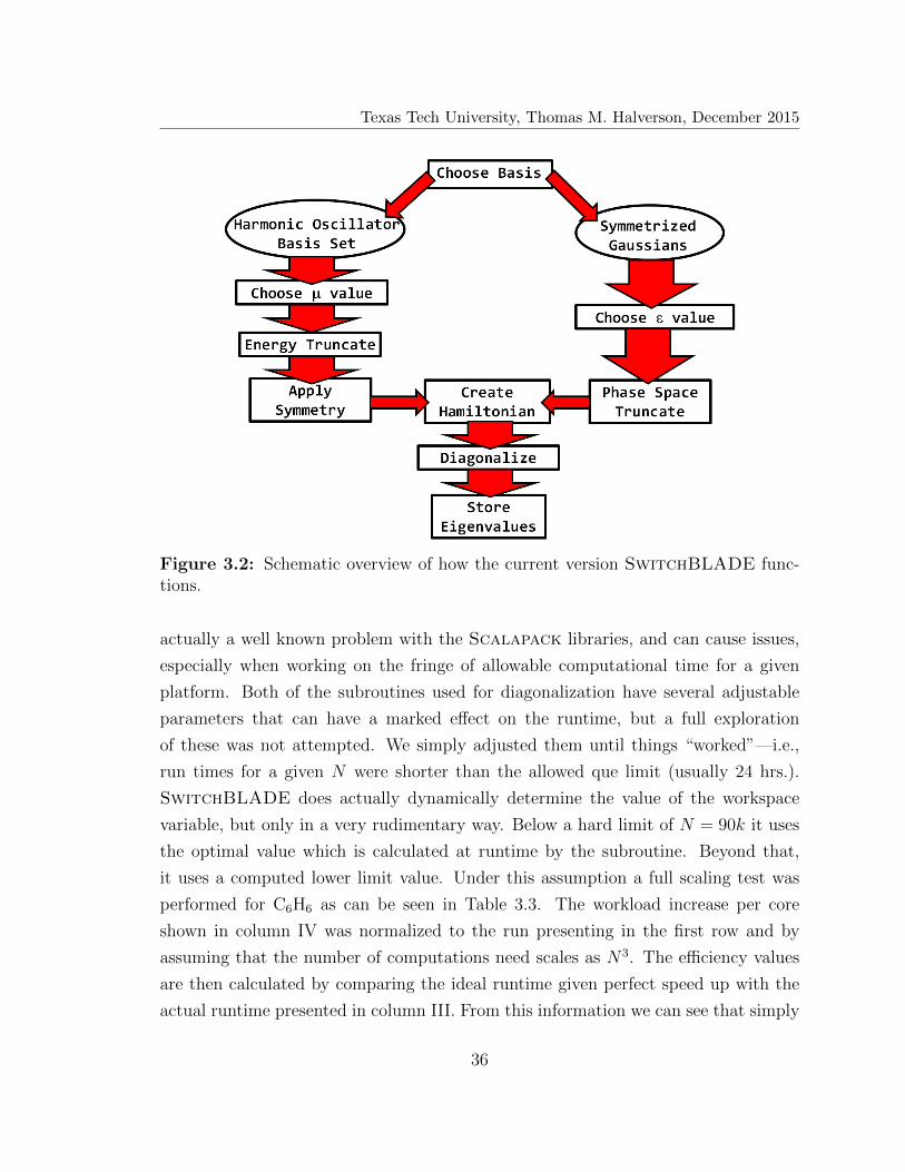
Texas Tech University, Thomas M. Halverson, December 2015
Figure 3.2: Schematic overview of how the current version SwitchBLADE func-tions.
actually a well known problem with the Scalapack libraries, and can cause issues,
especially when working on the fringe of allowable computational time for a given
platform. Both of the subroutines used for diagonalization have several adjustable
parameters that can have a marked effect on the runtime, but a full exploration
of these was not attempted. We simply adjusted them until things “worked”—i.e.,
run times for a given N were shorter than the allowed que limit (usually 24 hrs.).
SwitchBLADE does actually dynamically determine the value of the workspace
variable, but only in a very rudimentary way. Below a hard limit of N = 90k it uses
the optimal value which is calculated at runtime by the subroutine. Beyond that,
it uses a computed lower limit value. Under this assumption a full scaling test was
performed for C6H6 as can be seen in Table 3.3. The workload increase per core
shown in column IV was normalized to the run presenting in the first row and by
assuming that the number of computations need scales as N3. The efficiency values
are then calculated by comparing the ideal runtime given perfect speed up with the
actual runtime presented in column III. From this information we can see that simply
36
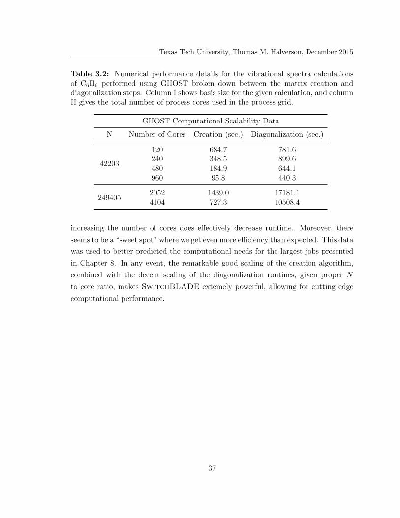
Texas Tech University, Thomas M. Halverson, December 2015
Table 3.2: Numerical performance details for the vibrational spectra calculationsof C6H6 performed using GHOST broken down between the matrix creation anddiagonalization steps. Column I shows basis size for the given calculation, and columnII gives the total number of process cores used in the process grid.
GHOST Computational Scalability Data
N Number of Cores Creation (sec.) Diagonalization (sec.)
42203
120 684.7 781.6240 348.5 899.6480 184.9 644.1960 95.8 440.3
2494052052 1439.0 17181.14104 727.3 10508.4
increasing the number of cores does effectively decrease runtime. Moreover, there
seems to be a “sweet spot” where we get even more efficiency than expected. This data
was used to better predicted the computational needs for the largest jobs presented
in Chapter 8. In any event, the remarkable good scaling of the creation algorithm,
combined with the decent scaling of the diagonalization routines, given proper N
to core ratio, makes SwitchBLADE extemely powerful, allowing for cutting edge
computational performance.
37
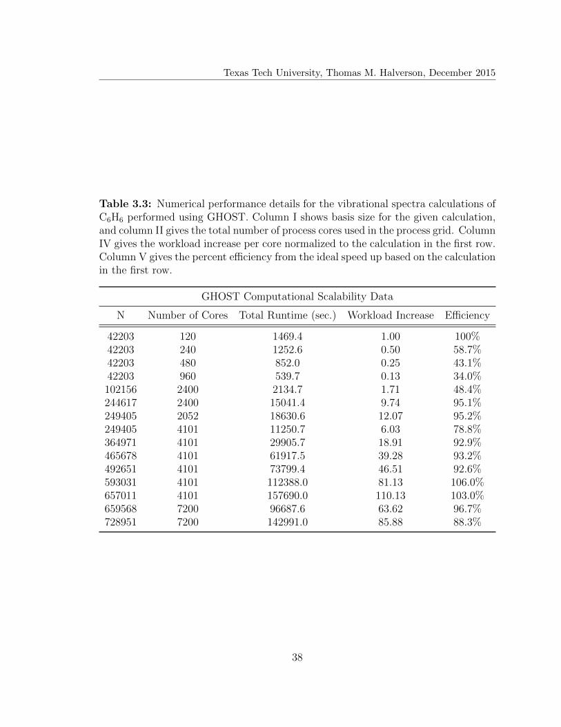
Texas Tech University, Thomas M. Halverson, December 2015
Table 3.3: Numerical performance details for the vibrational spectra calculations ofC6H6 performed using GHOST. Column I shows basis size for the given calculation,and column II gives the total number of process cores used in the process grid. ColumnIV gives the workload increase per core normalized to the calculation in the first row.Column V gives the percent efficiency from the ideal speed up based on the calculationin the first row.
GHOST Computational Scalability Data
N Number of Cores Total Runtime (sec.) Workload Increase Efficiency
42203 120 1469.4 1.00 100%42203 240 1252.6 0.50 58.7%42203 480 852.0 0.25 43.1%42203 960 539.7 0.13 34.0%102156 2400 2134.7 1.71 48.4%244617 2400 15041.4 9.74 95.1%249405 2052 18630.6 12.07 95.2%249405 4101 11250.7 6.03 78.8%364971 4101 29905.7 18.91 92.9%465678 4101 61917.5 39.28 93.2%492651 4101 73799.4 46.51 92.6%593031 4101 112388.0 81.13 106.0%657011 4101 157690.0 110.13 103.0%659568 7200 96687.6 63.62 96.7%728951 7200 142991.0 85.88 88.3%
38

Texas Tech University, Thomas M. Halverson, December 2015
CHAPTER 4
DIMENSIONAL SCALING AND PROOF OF CONCEPT
4.1 Isotropic Uncoupled Harmonic Oscillators (IUHO’s)
IUHO’s provide a convenient starting point to benchmark the utility of any EQD
method. This is especially true for the SGB approach, because exact solutions are
known and dimensional scalability analysis is straightforward. Poirier and coworkers
considered IUHO’s up to D= 15 to explicitly demonstrate that a PST-weylet basis
defeats exponential scaling.19,21 In their analysis, they considered both integer (ε = 0)
and half-integer (ε = 1/2) m grids. We present similar calculations (identical Emax
and N values) for IUHO’s from D=5 to D=11 on half-integer m grids. For the larger
D calculations, D = 12 to D = 15, we use an integer m grid, to mitigate the large
jumps in N that occur as Emax is increased.21 Such a limitation only applies to IUHO
systems—i.e., the greatly reduced symmetry of more realistic potentials results in far
less sizable jumps. We also present results for IUHO’s at higher D values (D=15 to
D=27), as well as lower D calculations with larger Emax (and therefore larger N and
K) values than considered in previous weylet studies.
The IUHO’s used here are defined by Eq. (2.2), setting ωi = 1, kijl = 0, and
kijln = 0. The eigenenergies for this system are well known and are given by
E(D)ν = (ν +
D
2) ; ν ∈ {0, 1, 2, ...}, (4.1)
where ν is the energy level. The degeneracy for each level is given by
deg(ν,D) =
(ν +D − 1
D − 1
). (4.2)
Our analysis presumes that for a typical spectroscopy calculation, we are inter-
esting in total excitations of ∼ 10 vibrational quanta, to be distributed across all of
the available modes. This corresponds to a typical energy scale for a given problem.
Next, we define a desired accuracy for the computed energy eigenvalues, expressed
as a fraction of the above energy scale; Poirier and Salam made arguments for 2%
accuracy being a reasonable target for an efficient weylet calculation,21 but they also
extended their analysis to higher accuracies. Here, we consider two different accura-
39

Texas Tech University, Thomas M. Halverson, December 2015
cies: 2% and 0.2%. Thus, a computed eigenenergy is accurate to within 2% (0.2%)
if it falls within 0.2 × D (0.02 × D) of the exact analytical value. At higher D, we
relaxed our tolerance to 3% to explore the “efficiency cliff” phenomenon22 (discussed
below).
Table 4.1 indicates the number of accurately computed eigenenergies, K, as a
function of Emax, for D = 5. For the most part, the performance of the SGB and
weylet basis sets is very similar, with weylets performing slightly better at the larger
Emax values. However, there are some marked differences at the 0.2% accuracy level.
This can best be understood in terms of what we call the “efficiency cliff”, based on
the observation that all calculations exhibit a narrow Emax range over which (K/N)
increases very sharply. The precise location of this cliff depends on the accuracy
level, and to a lesser degree, the choice of basis—i.e., weylet or SGB. In Table 4.1, for
example, at 0.2% accuracy the efficiency of weylets increases by an order of magnitude
from Emax = 10.5 to Emax = 13.5, while the change of efficiency for the SGB is
negligible. In this range, weylets are climbing the cliff, while the SGB is not. On
the other hand, the SGB experience an order of magnitude increase in efficiency
from Emax = 13.5 to Emax = 16.5, where the efficiency of weylets remains relatively
constant, meaning the SGB is now climbing the cliff. Thus, what appear to be large
differences in performance are merely relatively minor displacements in the location
of the respective efficiency cliffs.
As D increases, we observe the same trends. Table 4.2–Table 4.4 show that for
most of the allowable N values, the SGB and weylets yield the same K values at
2% accuracy. To the limited extent that the 0.2% cliff is being climbed at these
small N values, it appears that weylets again reach the cliff sooner. However, we
see in Table 4.5 that at D=10, the SGB cliff occurs sooner than weylets, leading to
dramatically better performance. The D=11 behavior is also somewhat anomalous,
for reasons that are not yet clear.
For larger D, the earlier trends resume, and we see that the weylet and SGB
performance is very similar at both 2.0% and 0.2%. Here, however, we do an ex-
plicit investigation of the efficiency cliff phenomenon by decreasing the error tolerance
slightly, from 2.0% to 3.0%. This yields a dramatic increase in the number of accurate
states for both basis sets. Table 4.6 shows results for D=12, D=13, D=15, and also
40

Texas Tech University, Thomas M. Halverson, December 2015
Table 4.1: Number of accurate eigenstates computed for D = 5 IUHO using theSGB compared with those previously computed using orthonormal weylets.21 Thenew SGB states were computed using the same energy cutoff values and the samehalf-integer m grid as the previous weylet calculations. The energy cutoff valuesyielded the same truncated basis sizes for both basis sets, but the number of accuratestates varied slightly between the two.
K for D = 5 IUHO
WeyletsSymmetrized
Gaussians
Emax N 2.0% 0.2% 2.0% 0.2%
4.0 32 0 0 0 07.5 352 30 0 30 010.5 1792 285 1 305 013.5 5952 1069 31 1054 116.5 15552 3003 127 2823 50
larger D values for the SGB only. The increase in K associated with this rather mod-
est decrease in accuracy is an astonishing two orders of magnitude or so, across the
board. This is another manifestation of the efficiency cliff phenomenon—i.e., there
are many states that lie not far beyond 2.0% convergence. This is likely due, in part,
to the high degeneracy of the IUHO model. Because of the large N jumps, we are
unable to “tune” our basis to converge the many states that are just out of reach; we
can only tune the accuracy threshold itself.
On the other hand, we can improve the actual accuracy of the computed eigenen-
ergies very substantially, using a simple rescaling procedure. Since it is known that
the computed energies are always too large (our approach satisfies a variational prin-
ciple), we can rescale by taking a ratio of the actual ground state to the computed
ground state, which reduces all computed eigenenergy values by a fixed percentage.
This procedure is justified by the fact that Monte Carlo methods can be used to ob-
tain highly accurate ground state energies even at large D. The rescaled values seen
in Table 4.6 illuminate how the rescaling method can be used to achieve good perfor-
mance at much lower threshold tolerances. For example, for D= 19, the SGB yields
41

Texas Tech University, Thomas M. Halverson, December 2015
Table 4.2: Comparison between the number of accurate states computed usingweylets and the SGB for D = 6 IUHO (consult Table 4.1 for further details).
K for D = 6 IUHO
WeyletsSymmetrized
Gaussians
Emax N 2.0% 0.2% 2.0% 0.2%
5.0 64 0 0 0 08.0 832 56 0 56 011.0 5056 624 0 589 014.5 19904 2910 22 2793 1
Table 4.3: Comparison between the number of accurate states computed usingweylets and the SGB for D = 7 IUHO (consult Table 4.1 for further details).
K for D = 7 IUHO
WeyletsSymmetrized
Gaussians
Emax N 2.0% 0.2% 2.0% 0.2%
5.5 128 0 0 0 09.0 1920 98 0 98 012.0 13568 1276 0 1269 0
Table 4.4: Comparison between the number of accurate states computed usingweylets and the SGB for D = 8 IUHO (consult Table 4.1 for further details).
K for D = 8 IUHO
WeyletsSymmetrized
Gaussians
Emax N 2.0% 0.2% 2.0% 0.2%
6.5 256 0 0 0 09.5 4352 174 0 174 013.0 35072 2461 1 2461 0
42
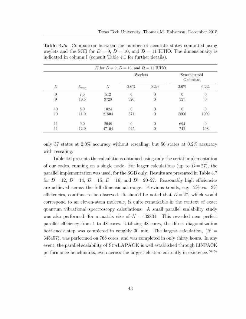
Texas Tech University, Thomas M. Halverson, December 2015
Table 4.5: Comparison between the number of accurate states computed usingweylets and the SGB for D = 9, D = 10, and D = 11 IUHO. The dimensionaity isindicated in column I (consult Table 4.1 for further details).
K for D = 9, D = 10, and D = 11 IUHO
Weylets SymmetrizedGaussians
D Emax N 2.0% 0.2% 2.0% 0.2%
9 7.5 512 0 0 0 09 10.5 9728 326 0 327 0
10 8.0 1024 0 0 0 010 11.0 21504 571 0 5606 1909
11 9.0 2048 0 0 694 011 12.0 47104 945 0 742 198
only 37 states at 2.0% accuracy without rescaling, but 56 states at 0.2% accuracy
with rescaling.
Table 4.6 presents the calculations obtained using only the serial implementation
of our codes, running on a single node. For larger calculations (up to D = 27), the
parallel implementation was used, for the SGB only. Results are presented in Table 4.7
for D = 12, D = 14, D = 15, D = 16, and D = 20–27. Reasonably high efficiencies
are achieved across the full dimensional range. Previous trends, e.g. 2% vs. 3%
efficiencies, continue to be observed. It should be noted that D = 27, which would
correspond to an eleven-atom molecule, is quite remarkable in the context of exact
quantum vibrational spectroscopy calculations. A small parallel scalability study
was also performed, for a matrix size of N = 32831. This revealed near perfect
parallel efficiency from 1 to 48 cores. Utilizing 48 cores, the direct diagonalization
bottleneck step was completed in roughly 30 min. The largest calculation, (N =
345457), was performed on 768 cores, and was completed in only thirty hours. In any
event, the parallel scalability of ScaLAPACK is well established through LINPACK
performance benchmarks, even across the largest clusters currently in existence.56–58
43

Texas Tech University, Thomas M. Halverson, December 2015
Table 4.6: Comparison between the number of accurate states computed usingweylets and the SGB for D = 12 to D = 19 IUHO. All results shown we computedusing serial codes. The dimension is indicated in column I. All calculations for bothbasis sets were performed using an integer m grid. The absence of data for weyletsindicates that no previous calculations were performed. Columns VI and IX refer tothe rescaled eigenvalues.
K for D = 12 to D = 19 IUHO
Weylets SymmetrizedGaussians
D Emax N 3.0% 2.0% 0.2%* 3.0% 2.0% 0.2%*
12 11.0 13527 1103 90 11 1103 90 3512 13.0 62103 - - - 5228 496 189
13 11.5 18578 1405 92 12 1405 92 3813 13.5 92158 - - - 6811 610 103
14 12.0 24942 1794 106 13 1758 28 4115 12.5 32831 2151 30 14 2152 30 4416 13.0 42473 - - - 2514 32 4717 13.0 54112 - - - 3027 34 5018 13.5 68008 - - - 3607 35 5319 14.0 84437 - - - 4257 37 56
* Rescaled
4.2 Coupled Anharmonic Oscillators (CAHO’s)
The CAHO Hamiltonian is obtained from Eq. (2.2) with ωj = 1.0, kijl = 0, and
kijln = 0 except for the terms, kiijj = βij and kiiii = αi. The presence of anharmonicity
and mode coupling is of course essential for modeling real molecules. There is no
theoretical reason why the SGB approach should work less well in this context than
for the IUHO, although some authors have claimed otherwise.59 In fact, the reduced
symmetry of the CAHO potential should alleviate the large jumps in N , leading to
a de facto improvement in efficiency. In any event, to establish a benchmark, we
compute SGB results for a range of anharmonicity and coupling strengths (α’s and
β’s) ranging from zero to very strong.
44
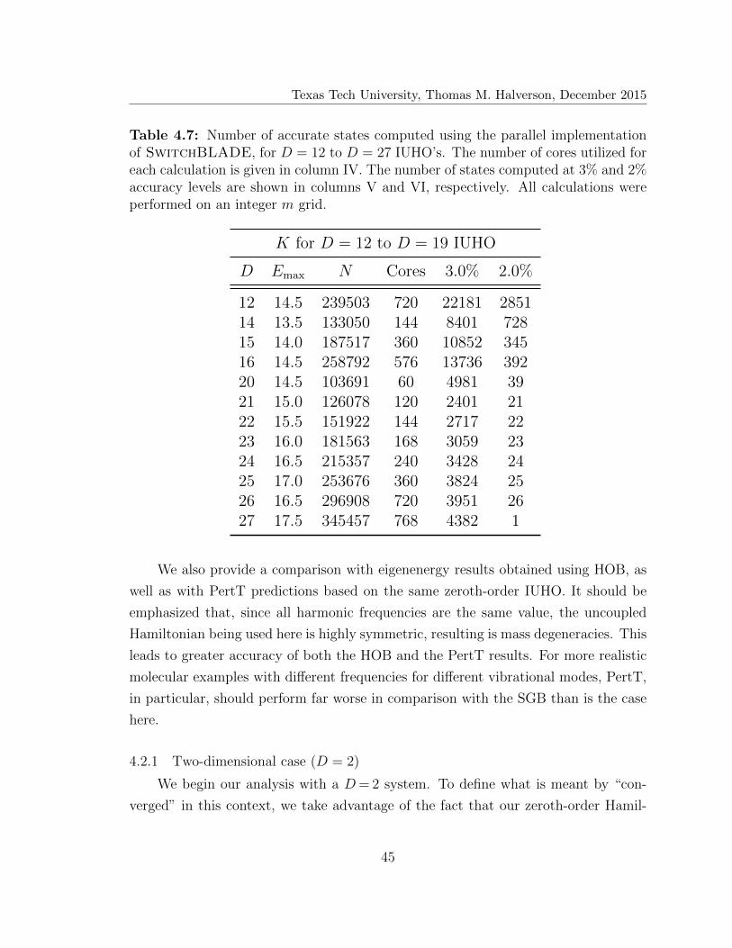
Texas Tech University, Thomas M. Halverson, December 2015
Table 4.7: Number of accurate states computed using the parallel implementationof SwitchBLADE, for D = 12 to D = 27 IUHO’s. The number of cores utilized foreach calculation is given in column IV. The number of states computed at 3% and 2%accuracy levels are shown in columns V and VI, respectively. All calculations wereperformed on an integer m grid.
K for D = 12 to D = 19 IUHO
D Emax N Cores 3.0% 2.0%
12 14.5 239503 720 22181 285114 13.5 133050 144 8401 72815 14.0 187517 360 10852 34516 14.5 258792 576 13736 39220 14.5 103691 60 4981 3921 15.0 126078 120 2401 2122 15.5 151922 144 2717 2223 16.0 181563 168 3059 2324 16.5 215357 240 3428 2425 17.0 253676 360 3824 2526 16.5 296908 720 3951 2627 17.5 345457 768 4382 1
We also provide a comparison with eigenenergy results obtained using HOB, as
well as with PertT predictions based on the same zeroth-order IUHO. It should be
emphasized that, since all harmonic frequencies are the same value, the uncoupled
Hamiltonian being used here is highly symmetric, resulting is mass degeneracies. This
leads to greater accuracy of both the HOB and the PertT results. For more realistic
molecular examples with different frequencies for different vibrational modes, PertT,
in particular, should perform far worse in comparison with the SGB than is the case
here.
4.2.1 Two-dimensional case (D = 2)
We begin our analysis with a D= 2 system. To define what is meant by “con-
verged” in this context, we take advantage of the fact that our zeroth-order Hamil-
45

Texas Tech University, Thomas M. Halverson, December 2015
tonian is an IUHO. This allows us to use the same 2% error tolerance as was used
previously. However in this case, we cannot compare calculated values to analytical
values. Instead, we exploit the fact that the SGB approach is variational, and com-
pute the difference between two sets of calculated values, one at Emax and one at
1.1 × Emax. The subset of eigenvalues for which this difference is less than the tol-
erance are said to be converged to within 2%, for the energy Emax. (This somewhat
simplistic criterion is introduced to enable facile comparisons across D values; a more
comprehensive convergence analysis is provided in Section 4.2.4.)
Also different from the IUHO calculations: instead of determiningK as a function
of N , we increase N (Emax) until a predetermined number of states, L, are converged.
With a maximum of 10 excitation quanta as presumed earlier, the target L value is
given exactly by a multinomial expansion, which we approximate here via
L ≈ 10D
D!. (4.3)
This yields L≈ 50 for D= 2. It should be noted that this approximation [Eq. (4.3)]
to the multinomial expansion begins to fail around D≈ 8, since the factorial in the
denominator grows faster that the exponential. However, only systems up to D= 4
will be analyzed using Eq. (4.3); the higher dimensional systems will be treated in a
different manner.
The main focus of this comparison is to see how the SGB and PertT methods
perform as the anharmonicity and coupling constants are varied. Figure 4.1 shows
that when the three perturbation parameters (α1, α2, and β) are set to zero, PertT
gives the exact analytical values, but the SGB does not, which is to be expected.
46
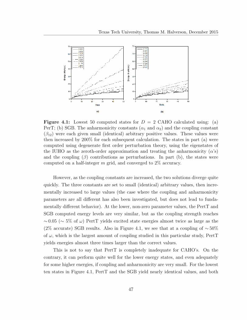
Texas Tech University, Thomas M. Halverson, December 2015
Figure 4.1: Lowest 50 computed states for D = 2 CAHO calculated using: (a)PerT; (b) SGB. The anharmonicity constants (α1 and α2) and the coupling constant(β12) were each given small (identical) arbitrary positive values. These values werethen increased by 200% for each subsequent calculation. The states in part (a) werecomputed using degenerate first order perturbation theory, using the eigenstates ofthe IUHO as the zeroth-order approximation and treating the anharmonicity (α’s)and the coupling (β) contributions as perturbations. In part (b), the states werecomputed on a half-integer m grid, and converged to 2% accuracy.
However, as the coupling constants are increased, the two solutions diverge quite
quickly. The three constants are set to small (identical) arbitrary values, then incre-
mentally increased to large values (the case where the coupling and anharmonicity
parameters are all different has also been investigated, but does not lead to funda-
mentally different behavior). At the lower, non-zero parameter values, the PertT and
SGB computed energy levels are very similar, but as the coupling strength reaches
∼ 0.05 (∼ 5% of ω) PertT yields excited state energies almost twice as large as the
(2% accurate) SGB results. Also in Figure 4.1, we see that at a coupling of ∼ 50%
of ω, which is the largest amount of coupling studied in this particular study, PertT
yields energies almost three times larger than the correct values.
This is not to say that PertT is completely inadequate for CAHO’s. On the
contrary, it can perform quite well for the lower energy states, and even adequately
for some higher energies, if coupling and anharmonicity are very small. For the lowest
ten states in Figure 4.1, PertT and the SGB yield nearly identical values, and both
47

Texas Tech University, Thomas M. Halverson, December 2015
capture the degeneracy pattern for those lower states. For the higher states, though,
the SGB results continue to display the same degeneracy pattern as for the lower
states, a feature that PertT fails to capture even qualitatively.
4.2.2 Three-dimensional case (D = 3)
The main difference between D= 2 and D= 3 is that there are now six pertur-
bation parameters—i.e., three anharmonicity constants (α1, α2, and α3) and three
coupling constants (β12, β13, and β23). This presents a large number of possible ways
to analyze the eigenvalues, with respect to variations in the α’s and β’s. An extensive
analysis of how the change of these parameters affects the energies was performed,
but a detailed presentation is excluded here. Instead, we focus on the case where all
constants are given the same value, which is increased simultaneously. This particular
case should demonstrate the best performance for PertT, and it will also allow for
better cross dimensional comparisons.
By employing Eq. (4.3) for D = 3, we sought to converge L≈ 150 states using
the same convergence scheme outlined in Section 4.2.1. We know that the amount
of degeneracy for a D = 3 IUHO [given by Eq. (4.2)] is large. This can be seen in
Figure 4.2, where the zero coupling (IUHO limit) is shown. In this limit, we know
that PertT gives the analytical values and the proper degeneracy. However, at higher
coupling values, it both overestimates the energy by close to a factor of three for
the higher states, and loses the degeneracy pattern exhibited by the accurate SGB
results.
4.2.3 Four-dimensional case (D = 4)
The largest dimensionality for which reasonable comparisons with PertT can
be made is D = 4. Because of the multiple degrees of freedom, there are now four
anharmonicity and six coupling constants. Along with this increase, Eq. (4.3) yields
L ≈ 400. As for the other D values, we do not report the full analysis that was
done with respect to the possible combinations of the α’s and β’s, but focus on the
case where all constants are the same. The results presented in Figure 4.3 exhibit
a continuation of earlier trends. At zero coupling, PertT gives the exact analytical
values and the proper degeneracy, similar to D = 3. For very small coupling—i.e.,
48
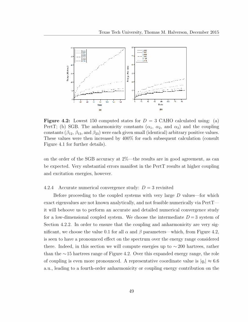
Texas Tech University, Thomas M. Halverson, December 2015
Figure 4.2: Lowest 150 computed states for D = 3 CAHO calculated using: (a)PertT; (b) SGB. The anharmonicity constants (α1, α2, and α3) and the couplingconstants (β12, β13, and β23) were each given small (identical) arbitrary positive values.These values were then increased by 400% for each subsequent calculation (consultFigure 4.1 for further details).
on the order of the SGB accuracy at 2%—the results are in good agreement, as can
be expected. Very substantial errors manifest in the PertT results at higher coupling
and excitation energies, however.
4.2.4 Accurate numerical convergence study: D = 3 revisited
Before proceeding to the coupled systems with very large D values—for which
exact eigenvalues are not known analytically, and not feasible numerically via PertT—
it will behoove us to perform an accurate and detailed numerical convergence study
for a low-dimensional coupled system. We choose the intermediate D= 3 system of
Section 4.2.2. In order to ensure that the coupling and anharmonicity are very sig-
nificant, we choose the value 0.1 for all α and β parameters—which, from Figure 4.2,
is seen to have a pronounced effect on the spectrum over the energy range considered
there. Indeed, in this section we will compute energies up to ∼ 200 hartrees, rather
than the ∼15 hartrees range of Figure 4.2. Over this expanded energy range, the role
of coupling is even more pronounced. A representative coordinate value is |qi| ≈ 6.6
a.u., leading to a fourth-order anharmonicity or coupling energy contribution on the
49

Texas Tech University, Thomas M. Halverson, December 2015
Figure 4.3: Lowest 400 computed states for D = 4 CAHO calculated using: (a)PertT; (b) SGB. The coupling constants (α1, α2, α3, and α4) and the anharmonicityconstants (β21, β13, β14, β23, β24, and β34) were each given small (identical) arbi-trary positive values. These values were then increased by 400% for each subsequentcalculation (consult Figure 4.1 for further details).
order of 0.1×6.64 ≈ 189 hartrees, which is on the scale of the entire expanded energy
range itself.
An accurate assessment of convergence first requires an accurate characterization
of the exact eigenvalues, for comparison. Since the system is coupled, these can only
be determined numerically. For the lower-lying eigenstates, an extremely efficient
choice of basis set is the zeroth-order IUHO basis set—i.e., HOB—because the cou-
pling perturbation is small in the low energy regime. We further optimize the HOB
by applying energetic truncation with µ = 0.0 as outlined in Section 2.4. According
to the previous analysis, this type of truncation should provide the best overall energy
eiegenstates at the bottom of the spectrum, provided we use a large enough N value
for our reference calculation.
As expected, the µ = 0.0 HOB calculation converges extremely rapidly for the
low-lying D=3 states, such that the first 150 eigenvalues are converged to at least five
digits past the decimal, for the largest basis size considered (N = 102340). Selected
eigenvalues are also presented in Table 4.8.
On the other hand, the higher-lying eigenvalues computed using this standard
method will not be well converged at all, and cannot be used as a reference for a
50
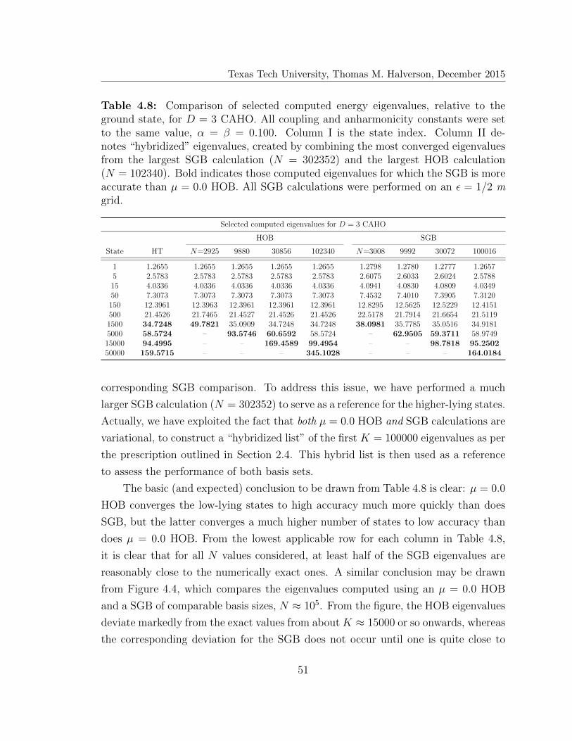
Texas Tech University, Thomas M. Halverson, December 2015
Table 4.8: Comparison of selected computed energy eigenvalues, relative to theground state, for D = 3 CAHO. All coupling and anharmonicity constants were setto the same value, α = β = 0.100. Column I is the state index. Column II de-notes “hybridized” eigenvalues, created by combining the most converged eigenvaluesfrom the largest SGB calculation (N = 302352) and the largest HOB calculation(N = 102340). Bold indicates those computed eigenvalues for which the SGB is moreaccurate than µ = 0.0 HOB. All SGB calculations were performed on an ε = 1/2 mgrid.
Selected computed eigenvalues for D = 3 CAHO
HOB SGB
State HT N=2925 9880 30856 102340 N=3008 9992 30072 100016
1 1.2655 1.2655 1.2655 1.2655 1.2655 1.2798 1.2780 1.2777 1.26575 2.5783 2.5783 2.5783 2.5783 2.5783 2.6075 2.6033 2.6024 2.578815 4.0336 4.0336 4.0336 4.0336 4.0336 4.0941 4.0830 4.0809 4.034950 7.3073 7.3073 7.3073 7.3073 7.3073 7.4532 7.4010 7.3905 7.3120150 12.3961 12.3963 12.3961 12.3961 12.3961 12.8295 12.5625 12.5229 12.4151500 21.4526 21.7465 21.4527 21.4526 21.4526 22.5178 21.7914 21.6654 21.51191500 34.7248 49.7821 35.0909 34.7248 34.7248 38.0981 35.7785 35.0516 34.91815000 58.5724 – 93.5746 60.6592 58.5724 – 62.9505 59.3711 58.974915000 94.4995 – – 169.4589 99.4954 – – 98.7818 95.250250000 159.5715 – – – 345.1028 – – – 164.0184
corresponding SGB comparison. To address this issue, we have performed a much
larger SGB calculation (N = 302352) to serve as a reference for the higher-lying states.
Actually, we have exploited the fact that both µ = 0.0 HOB and SGB calculations are
variational, to construct a “hybridized list” of the first K = 100000 eigenvalues as per
the prescription outlined in Section 2.4. This hybrid list is then used as a reference
to assess the performance of both basis sets.
The basic (and expected) conclusion to be drawn from Table 4.8 is clear: µ = 0.0
HOB converges the low-lying states to high accuracy much more quickly than does
SGB, but the latter converges a much higher number of states to low accuracy than
does µ = 0.0 HOB. From the lowest applicable row for each column in Table 4.8,
it is clear that for all N values considered, at least half of the SGB eigenvalues are
reasonably close to the numerically exact ones. A similar conclusion may be drawn
from Figure 4.4, which compares the eigenvalues computed using an µ = 0.0 HOB
and a SGB of comparable basis sizes, N ≈ 105. From the figure, the HOB eigenvalues
deviate markedly from the exact values from about K ≈ 15000 or so onwards, whereas
the corresponding deviation for the SGB does not occur until one is quite close to
51

Texas Tech University, Thomas M. Halverson, December 2015
the top end of the spectrum. The latter behavior would be most unusual for a
conventional basis, but is quite standard for a SGB.
In practice, for a coupled large D calculation, there may not be a hybrid list
against which to assess accuracy; one may be forced to simply compare a set of
smaller N calculations against a very large N calculation, regardless of the basis set
used. Ideally though, one could create a hybrid set from a myriad of calculations
with as large as N values as possible to create the “correct answer”. However, it
should be noted that one way to predict the accuracy of this method is to compare
the E0 state for each calculation, both intra- and inter-method. The former gives
a sense of the convergence of E0; the latter gives a sense of its accuracy. In the
limit as N→ inf, all exact methods, using the same PES, will converge to the same
E0. Here, we can see that the N values of both methods are almost large enough
for this to occur, since ESGB0 = 1.2657 and E0.0
0 = 1.2655 hartrees for the largest
calculations. However, E0 does not vary at all across all the µ = 0.0 HOB calculations,
but drops by 0.0141 hartrees for SGB. This is, somewhat, to be expected since we
know from Sections 2.2 and 2.4 that HOB performs better at the bottom of the
spectrum, especially when µ = 0.0. The extent to which this procedure may serve as
an estimate of a hypothetical comparison vs. the exact eigenvalues can be found in
Table 4.9. Here, the number of eigenvalues computed to a given level of accuracy for
different N ’s is presented. For the numbers without parentheses, the accuracies are
determined relative to the HT set, i.e. to the most converged numbers available. For
the SGB numbers in parentheses, accuracies are relative to the computed eigenvalues
obtained from the next largest SGB basis calculation. For all N values and accuracies,
the parenthetical numbers are the same order of magnitude as the non-parenthetical
values.
From the last two rows, we see that the parenthetical estimates are very good
for N≥105, for all but the highest 0.06% accuracy level, even though the N increase
is less than a factor of two. Note that the exact agreement in the last row should be
largely ignored, because for most states, the two comparisons are identical—although
this does justify the use of a very large N SGB calculation for convergence assessment
purposes. Likewise, the 0.06%, N≈105 µ = 0.0 HOB number is suspect, because the
relevant computed states are identical to those in the HT set. Table 4.9 also presents
52
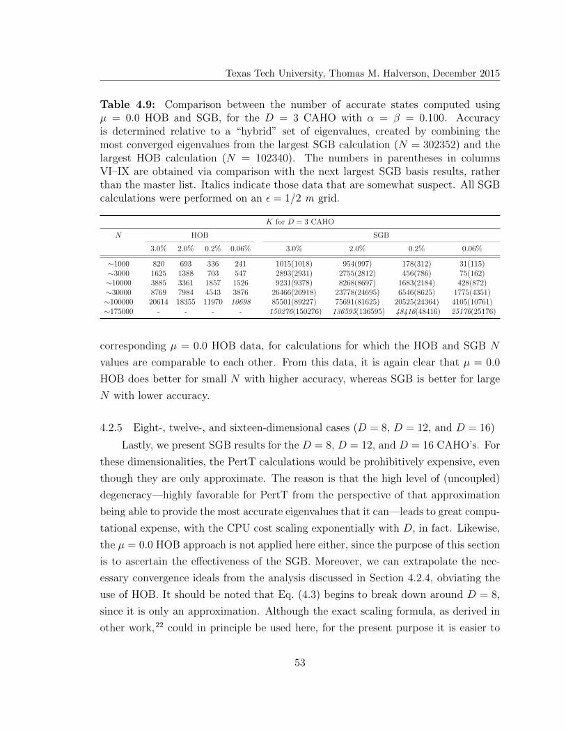
Texas Tech University, Thomas M. Halverson, December 2015
Table 4.9: Comparison between the number of accurate states computed usingµ = 0.0 HOB and SGB, for the D = 3 CAHO with α = β = 0.100. Accuracyis determined relative to a “hybrid” set of eigenvalues, created by combining themost converged eigenvalues from the largest SGB calculation (N = 302352) and thelargest HOB calculation (N = 102340). The numbers in parentheses in columnsVI–IX are obtained via comparison with the next largest SGB basis results, ratherthan the master list. Italics indicate those data that are somewhat suspect. All SGBcalculations were performed on an ε = 1/2 m grid.
K for D = 3 CAHO
N HOB SGB
3.0% 2.0% 0.2% 0.06% 3.0% 2.0% 0.2% 0.06%
∼1000 820 693 336 241 1015(1018) 954(997) 178(312) 31(115)∼3000 1625 1388 703 547 2893(2931) 2755(2812) 456(786) 75(162)∼10000 3885 3361 1857 1526 9231(9378) 8268(8697) 1683(2184) 428(872)∼30000 8769 7984 4543 3876 26466(26918) 23778(24695) 6546(8625) 1775(4351)∼100000 20614 18355 11970 10698 85501(89227) 75691(81625) 20525(24364) 4105(10761)∼175000 - - - - 150276(150276) 136595(136595) 48416(48416) 25176(25176)
corresponding µ = 0.0 HOB data, for calculations for which the HOB and SGB N
values are comparable to each other. From this data, it is again clear that µ = 0.0
HOB does better for small N with higher accuracy, whereas SGB is better for large
N with lower accuracy.
4.2.5 Eight-, twelve-, and sixteen-dimensional cases (D = 8, D = 12, and D = 16)
Lastly, we present SGB results for the D = 8, D = 12, and D = 16 CAHO’s. For
these dimensionalities, the PertT calculations would be prohibitively expensive, even
though they are only approximate. The reason is that the high level of (uncoupled)
degeneracy—highly favorable for PertT from the perspective of that approximation
being able to provide the most accurate eigenvalues that it can—leads to great compu-
tational expense, with the CPU cost scaling exponentially with D, in fact. Likewise,
the µ = 0.0 HOB approach is not applied here either, since the purpose of this section
is to ascertain the effectiveness of the SGB. Moreover, we can extrapolate the nec-
essary convergence ideals from the analysis discussed in Section 4.2.4, obviating the
use of HOB. It should be noted that Eq. (4.3) begins to break down around D = 8,
since it is only an approximation. Although the exact scaling formula, as derived in
other work,22 could in principle be used here, for the present purpose it is easier to
53
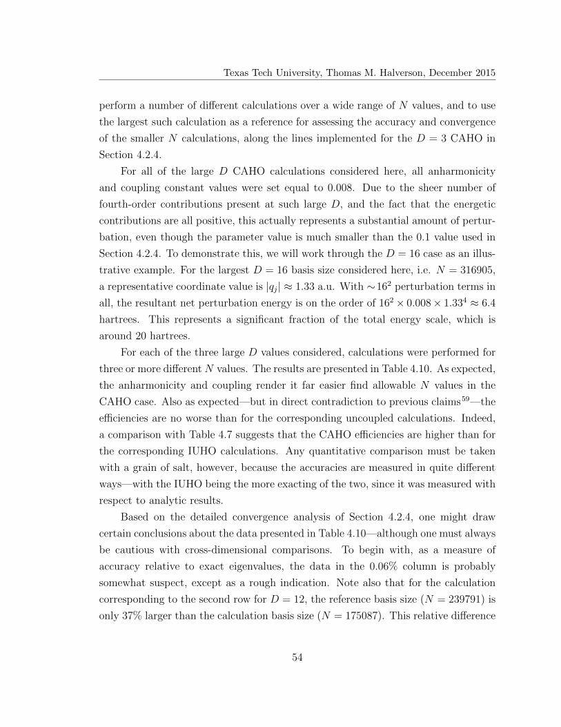
Texas Tech University, Thomas M. Halverson, December 2015
perform a number of different calculations over a wide range of N values, and to use
the largest such calculation as a reference for assessing the accuracy and convergence
of the smaller N calculations, along the lines implemented for the D = 3 CAHO in
Section 4.2.4.
For all of the large D CAHO calculations considered here, all anharmonicity
and coupling constant values were set equal to 0.008. Due to the sheer number of
fourth-order contributions present at such large D, and the fact that the energetic
contributions are all positive, this actually represents a substantial amount of pertur-
bation, even though the parameter value is much smaller than the 0.1 value used in
Section 4.2.4. To demonstrate this, we will work through the D = 16 case as an illus-
trative example. For the largest D = 16 basis size considered here, i.e. N = 316905,
a representative coordinate value is |qj| ≈ 1.33 a.u. With ∼162 perturbation terms in
all, the resultant net perturbation energy is on the order of 162× 0.008× 1.334 ≈ 6.4
hartrees. This represents a significant fraction of the total energy scale, which is
around 20 hartrees.
For each of the three large D values considered, calculations were performed for
three or more differentN values. The results are presented in Table 4.10. As expected,
the anharmonicity and coupling render it far easier find allowable N values in the
CAHO case. Also as expected—but in direct contradiction to previous claims59—the
efficiencies are no worse than for the corresponding uncoupled calculations. Indeed,
a comparison with Table 4.7 suggests that the CAHO efficiencies are higher than for
the corresponding IUHO calculations. Any quantitative comparison must be taken
with a grain of salt, however, because the accuracies are measured in quite different
ways—with the IUHO being the more exacting of the two, since it was measured with
respect to analytic results.
Based on the detailed convergence analysis of Section 4.2.4, one might draw
certain conclusions about the data presented in Table 4.10—although one must always
be cautious with cross-dimensional comparisons. To begin with, as a measure of
accuracy relative to exact eigenvalues, the data in the 0.06% column is probably
somewhat suspect, except as a rough indication. Note also that for the calculation
corresponding to the second row for D = 12, the reference basis size (N = 239791) is
only 37% larger than the calculation basis size (N = 175087). This relative difference
54
Texas Tech University, Thomas M. Halverson, December 2015
Table 4.10: Number of accurate states computed for D = 8, D = 12, and D = 16CAHO’s. All of the coupling and anharmonicity constants were set to the same value,α = β = 0.008. Accuracy is assessed via comparison with the largest calculationperformed for each D value (N = 350147 for D = 8; N = 239791 for D = 12; N =316905 for D = 16). The number of computational cores utilized for each calculationis given in column IV. Italics indicate those data that are somewhat suspect, if takenas a measure of accuracy relative to exact eigenvalues. All SGB calculations wereperformed on an integer m grid.
K for D = 8, D = 12, and D = 16 CAHO
D Emax N Cores 2.0% 0.2% 0.06%
8 14.5 23925 24 2408 0 08 18.0 154323 576 88320 128 08 19.0 211251 1152 160713 652 18 19.5 242627 1728 203946 2359 11
12 14.5 79759 144 66890 12 012 15.5 175087 1728 168421 21932 3128
16 13.0 13321 36 8265 0 016 14.0 42473 60 32023 0 016 15.0 117993 576 110264 239 0
is substantially smaller than all of the others considered in this table and in Table 4.9,
which might account for the anomalously large 0.2% value obtained here. All in all,
though, these results are very encouraging. Even for the N = 117993, D = 16
calculation, for instance, most of the computed eigenvalues are 2% accurate, and a
good number are likely accurate to 0.2% as well.
4.3 Conclusions
From the above study, it can be tempting to imagine that any problem can
be solved via some suitable numerical technique, especially from a pure theoretical
standpoint. However, in practice this is far from being the case. Many subtle pit-
falls exist that can render the use of numerical solution techniques arduous, if not
intractible. The main pitfall explored here is, of course, exponential scaling, which
proves to be quite an obstacle. It does, however, motivate the creation of fresh, in-
55
Texas Tech University, Thomas M. Halverson, December 2015
novative techniques to defeat this formidable opponent. Here, we have shown that
the SGB approach allows us to create a basis that is amenable to PST, which ergo
defeats exponential scaling. By utilizing the SGB, we are able to perform accurate
calculations on systems up to D = 27, setting a new benchmark for basis set ex-
pansion methods in time-independent quantum dynamics. We have examined both
uncoupled and coupled cases, and shown that the latter are at least as efficient as the
former, vis-a-vis (K/N) ratios, especially for the higher dimensionalities considered.
We have implemented all of this using a massively parallel, dimension-independent
code, which is remarkably simple, and easy for non-experts to use. However, much
work remains to be done.
The thresholds of accuracy explored here were chosen because they lead to a
reasonably efficient calculation, measured as the K/N ratio. However, this does
not represent a high level of accuracy, certainly far less than what can be called
“spectroscopic accuracy”. That is not to say that higher levels of accuracy cannot
be achieved using this method, but to compute a large number of states to very high
accuracy requires extremely large N values—or low K/N ratios—at large D, which is
a known disadvantage of the current incarnation of this approach.20 However, there
is a fix. One way to avert the use of very large matrices, and still greatly increase the
accuracy, is to apply the phase space region operator (PSRO) method developed by
Lombardini and Poirier.22 This would utilize specialized projection operators13,14 to
transform the initial SGB, into a customized basis specifically tailored for the given
system. Using the PSRO method, Lombardini and Poirier were able to increase the
computed accuracy level to a very high degree—i.e., to what could be called true
spectroscopic accuracy—while still maintaining relatively modest N values.
The PSRO method discussed above, though almost certainly quite beneficial
for providing very high accuracies at the lower dimensionalities, may not in practice
achieve such high accuracies at the higher dimensionalities in the range considered,
i.e. D ≈ 30. The main reason is that highly accurate PES’s for such systems are
not known. The inherent accuracy obtainable from a fourth-order Taylor expanded
potential is limited, even assuming that all of the relevant coupling and anharmonicity
constants are available. The total number of perturbation parameters for such large
56
Texas Tech University, Thomas M. Halverson, December 2015
D is in principle very large, but most of the parameter values will be inconsequentially
small.
Nevertheless, the proposed calculations are worth doing, for several reasons.
First, a computationally inexpensive form of PSRO may deliver an “intermediate”
level of accuracy (say, to one part in 104) at the large D values—commensurate with
the “ten wavenumber” accuracy of the fourth-order PES itself, but beyond the capa-
bilities of other current methods. In this context, the multi-configuration time depen-
dent Hartree (MCTDH) method15 is probably the only competing approach; however,
the MCTDH codes are orders of magnitude more complex than SwitchBLADE.
Second, PSRO enables calculation of a much larger number of accurately computed
K’s for a given N , even if the desired accuracy threshold is modest. Finally, at the
lower D values—say, D=10–30—modern techniques are rendering accurate PES de-
velopment possible, as a result of which spectroscopically accurate quantum dynamics
calculations are in demand (e.g., for malonaldehyde60). Such calculations can be per-
formed using PSRO SGB, provided an accurate Gaussian quadrature scheme is also
employed.51 This scheme has itself been carefully crafted so as to avoid exponential
scaling.
57
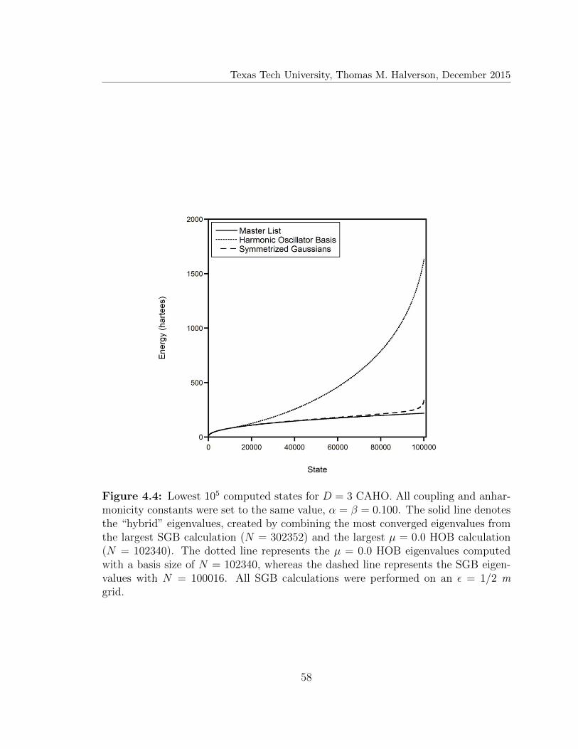
Texas Tech University, Thomas M. Halverson, December 2015
Figure 4.4: Lowest 105 computed states for D = 3 CAHO. All coupling and anhar-monicity constants were set to the same value, α = β = 0.100. The solid line denotesthe “hybrid” eigenvalues, created by combining the most converged eigenvalues fromthe largest SGB calculation (N = 302352) and the largest µ = 0.0 HOB calculation(N = 102340). The dotted line represents the µ = 0.0 HOB eigenvalues computedwith a basis size of N = 102340, whereas the dashed line represents the SGB eigen-values with N = 100016. All SGB calculations were performed on an ε = 1/2 mgrid.
58

Texas Tech University, Thomas M. Halverson, December 2015
CHAPTER 5
DIPHOSPHOROUS OXIDE (D = 3)
Our primary interest in P2O is as a simple benchmark triatomic system for which
an FFP exists.61,62 Through the years, phosphorous compounds have been studied in
astrophysics, particularly those serving as reaction intermediates.63,64 More recently,
P2O5 has become a concern in the production of more environmentally safe steel and
steel alloys.65 These applications serve as examples as to why accurate spectroscopic
data for compounds such as P2O could have interesting implications across many
scientific fields. It should be noted that the low D of P2O lends itself quite well to
other exact quantum methods, e.g. DVR methods, and systems of this size have been
studied using such methods many times.12 However, even for such a small system,
PSLB methods can prove useful—especially if a large number of excited states is
desired.
Using SwitchBLADE, we computed the vibrational energy levels of P2O, as-
sociated with the FFP by Pouchan et al, which is of the form in Eq. (2.2).61 This
FFP was obtained via a least squares fit method with an RMS fit error of ∼ 0.3
cm−1. Despite this, the agreement with experimental spectra (∼ 10 cm−1) is not par-
ticularly good even for the fundamental transitions, suggesting an FFP of somewhat
limited quality. Although a much better (in the sense of agreement with experiment)
P2O FFP does exist,62 the Pouchan FFP serves our present purpose of providing
a realistic test case model for evaluating SGB method performance. For a system
this small, there is no need to utilize HOB, since the SGB alone yield L ≈ 300 to
sub-wavenumber accuracy.
Using their own FFP, Pouchan et al. computed some vibrational energies, up
to the third excitation of mode three (3ν3). These values, which were reported to be
converged to 1 cm−1, can be seen in column IV of Table 5.1. Places in the column
where no value is shown are states that were not calculated by Pouchan et al., most
likely due to their truncation scheme not allowing for sufficiently high excitations
in a single mode (specifically, mode j = 1). In contrast, since our calculations are
PST-based, we do not have issues with large overtones—i.e., our calculations yield
a complete spectrum. Columns II and III in Table 5.1 depict the P2O energies we
59

Texas Tech University, Thomas M. Halverson, December 2015
calculated using SwitchBLADE. Results for both the largest basis set calculation
(N ∼ 400, 000) and the second largest (N ∼ 200, 000) are reported, in order to
demonstrate the level of numerical convergence achieved (between a few 0.001 cm−1
and a few 0.1 cm−1) throughout the energy range indicated. All of our calculated
energies agree with those from Ref. 61 to within ∼ 1 cm−1.
For a system with small D, the calculation of the lowest lying 26 vibrational
states to < 10 cm−1—though it may represent spectroscopic accuracy—is certainly
less accurate than could be obtained using other means. However, numerically pre-
cise low-lying energy eigenstates was never the goal here. What was the goal was
to calculate the entire L range to at least ∼ 10 cm−1, which is easily done utiliz-
ing SwitchBLADE. Moreover, SwitchBLADE, armed with the SGB, also yields
many more states than just L. In Table 5.2, we present a selected number of states
up to the 10, 000th excitation. We can see that even at this high level of excitation,
which is on the order of the dissociation energy,66 the convergence accuracy is ∼ 10
cm−1. Though no longer spectroscopic, this is far more accurate than what can likely
be obtained using other methods. It should also be noted that all the calculations
were done only using the SGB, without the addition of the HOB. The ground state,
E0 = 1065.27 cm−1, is converged to 0.1 cm−1, obviated the use of the HOB since we
get the lowest states to better than our desired accuracy. Moreover, this initial test
system was investigated to test the viability of the SGB on a real system (one with
realistic anharmonicity), and utilizing HOB would be overkill.
As for the higher-lying states, of course, one cannot rely on eigenenergies com-
puted using any force field—even an accurate one—near the dissociation threshold.
Therefore, the 10, 000th excited state result has little value as an experimental predic-
tion. Nevertheless, it is quite valuable from the perspective of assessing the numerical
performance of the SGB approach. Note that for the larger D molecular systems of
the sort for which SwitchBLADE is primarily intended, the scaling of the density
of states is such that the 10, 000th excited state typically lies only a few thousand
cm−1 above ν1 = E1 − E0—i.e., well below the dissociation threshold. However, this
is still sufficiently excited that coupling and anharmonicity should play an extremely
important dynamical role. At such “intermediate” energies, even a very good FFP
60
Texas Tech University, Thomas M. Halverson, December 2015
may only be accurate to a ∼ 10 cm−1, which is on the same level of accuracy as the
SGB method itself.
The basis convergence pattern—seen in detail in Tables 5.2 and 5.3—is typical
of PSLB methods like SGB, but very different from other, more traditional methods.
This difference can be directly attributed to the fact that SGB utilizes PST, defeat-
ing exponential scaling—but without the underlying functions being customized to
the specific problem at hand. The main manifestation of this is that, for low-to-
intermediate accuracy levels, we obtain high (K/N) ratios (efficiencies). In fact, it is
only in the top half of the spectrum or so that the computed and exact energy eigen-
values begin to differ qualitatively. Thus, for example, the 10, 000th excited state
as computed using N = 12, 711 is off by ∼ 2000 cm−1, but by N = 105, 781, this
error reduces to ∼ 50 cm−1. This same behavior can be seen in Table 5.3, where we
show the number of converged states at varying levels of accuracy. Note that 26,084
states—a full 13%—are converged to within 10 cm−1. On the other hand, in Table 5.3
we also see that our method yields a relatively small (but still respectable) number
of spectroscopically accurate states, which is to be expected.
61
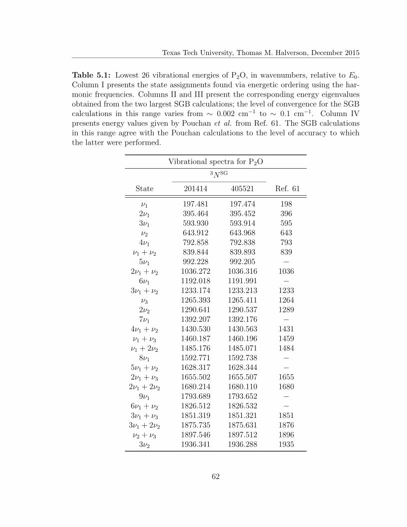
Texas Tech University, Thomas M. Halverson, December 2015
Table 5.1: Lowest 26 vibrational energies of P2O, in wavenumbers, relative to E0.Column I presents the state assignments found via energetic ordering using the har-monic frequencies. Columns II and III present the corresponding energy eigenvaluesobtained from the two largest SGB calculations; the level of convergence for the SGBcalculations in this range varies from ∼ 0.002 cm−1 to ∼ 0.1 cm−1. Column IVpresents energy values given by Pouchan et al. from Ref. 61. The SGB calculationsin this range agree with the Pouchan calculations to the level of accuracy to whichthe latter were performed.
Vibrational spectra for P2O
3NSG
State 201414 405521 Ref. 61
ν1 197.481 197.474 1982ν1 395.464 395.452 3963ν1 593.930 593.914 595ν2 643.912 643.968 6434ν1 792.858 792.838 793
ν1 + ν2 839.844 839.893 8395ν1 992.228 992.205 −
2ν1 + ν2 1036.272 1036.316 10366ν1 1192.018 1191.991 −
3ν1 + ν2 1233.174 1233.213 1233ν3 1265.393 1265.411 12642ν2 1290.641 1290.537 12897ν1 1392.207 1392.176 −
4ν1 + ν2 1430.530 1430.563 1431ν1 + ν3 1460.187 1460.196 1459ν1 + 2ν2 1485.176 1485.071 1484
8ν1 1592.771 1592.738 −5ν1 + ν2 1628.317 1628.344 −2ν1 + ν3 1655.502 1655.507 16552ν1 + 2ν2 1680.214 1680.110 1680
9ν1 1793.689 1793.652 −6ν1 + ν2 1826.512 1826.532 −3ν1 + ν3 1851.319 1851.321 18513ν1 + 2ν2 1875.735 1875.631 1876ν2 + ν3 1897.546 1897.512 1896
3ν2 1936.341 1936.288 1935
62
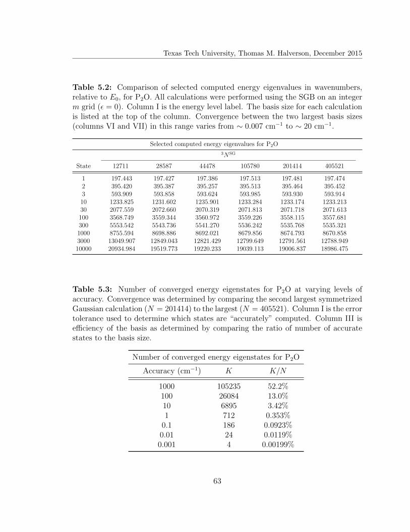
Texas Tech University, Thomas M. Halverson, December 2015
Table 5.2: Comparison of selected computed energy eigenvalues in wavenumbers,relative to E0, for P2O. All calculations were performed using the SGB on an integerm grid (ε = 0). Column I is the energy level label. The basis size for each calculationis listed at the top of the column. Convergence between the two largest basis sizes(columns VI and VII) in this range varies from ∼ 0.007 cm−1 to ∼ 20 cm−1.
Selected computed energy eigenvalues for P2O
3NSG
State 12711 28587 44478 105780 201414 405521
1 197.443 197.427 197.386 197.513 197.481 197.4742 395.420 395.387 395.257 395.513 395.464 395.4523 593.909 593.858 593.624 593.985 593.930 593.91410 1233.825 1231.602 1235.901 1233.284 1233.174 1233.21330 2077.559 2072.660 2070.319 2071.813 2071.718 2071.613100 3568.749 3559.344 3560.972 3559.226 3558.115 3557.681300 5553.542 5543.736 5541.270 5536.242 5535.768 5535.3211000 8755.594 8698.886 8692.021 8679.856 8674.793 8670.8583000 13049.907 12849.043 12821.429 12799.649 12791.561 12788.94910000 20934.984 19519.773 19220.233 19039.113 19006.837 18986.475
Table 5.3: Number of converged energy eigenstates for P2O at varying levels ofaccuracy. Convergence was determined by comparing the second largest symmetrizedGaussian calculation (N = 201414) to the largest (N = 405521). Column I is the errortolerance used to determine which states are “accurately” computed. Column III isefficiency of the basis as determined by comparing the ratio of number of accuratestates to the basis size.
Number of converged energy eigenstates for P2O
Accuracy (cm−1) K K/N
1000 105235 52.2%100 26084 13.0%10 6895 3.42%1 712 0.353%
0.1 186 0.0923%0.01 24 0.0119%0.001 4 0.00199%
63

Texas Tech University, Thomas M. Halverson, December 2015
CHAPTER 6
METHYLENEIMINE (D = 9)
Methyleneimine has been shown to be an important reaction intermediate in
many chemical processes.67 In particular, it plays an important role in both atmo-
spheric science and interstellar cloud formations.68 Despite its chemical importance,
the large dimensionality (D=9) of CH2NH makes EQD calculations difficult. It there-
fore represents another good benchmark for SwitchBLADE, as we move toward the
regime of the “very large”.
We calculated the vibrational spectra for CH2NH using the FFP given by Pouchan
and Zaki.69 However, some of the important computational details were omitted in
Ref. 69, and the FFP, as presented, leads to ambiguity in how the reported coefficients
are to be interpreted. The Hamiltonian equation we present in this paper [Eq. (2.2)],
adopts a constrained summation convention, and denotes the third and fourth order
force constants as k’s. Pouchan adopts what appears to be an unconstrained summa-
tion convention, labeling his constants as φ’s, but the precise meaning in that paper
is unclear.
Which convention is chosen for the reported values, constrained or unconstrained,
has a large effect on the amount of coupling that the system exhibits. If one treats
these coefficients as unconstrained, then the barrier height for dissociation drops
below the energy range of the states reported in Ref. 69. This can be seen in Fig-
ures 6.1 and 6.2, which show, respectively, the corresponding dissociation reaction
pathway and reaction profile. Indeed, an SGB calculation performed according to the
unconstrained interpretation of the presented coefficients led to nonsensical results.
If instead, we assume that the coefficients as presented in Ref. 69 are constrained,
then the barrier height becomes much higher, and it becomes possible to compute
meaningful bound state energy eigenvalues.
64
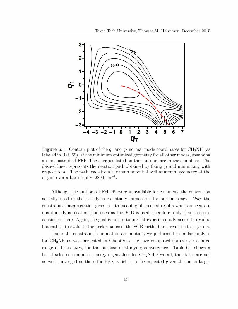
Texas Tech University, Thomas M. Halverson, December 2015
Figure 6.1: Contour plot of the q1 and q7 normal mode coordinates for CH2NH (aslabeled in Ref. 69), at the minimum optimized geometry for all other modes, assumingan unconstrained FFP. The energies listed on the contours are in wavenumbers. Thedashed lined represents the reaction path obtained by fixing q7 and minimizing withrespect to q1. The path leads from the main potential well minimum geometry at theorigin, over a barrier of ∼ 2800 cm−1.
Although the authors of Ref. 69 were unavailable for comment, the convention
actually used in their study is essentially immaterial for our purposes. Only the
constrained interpretation gives rise to meaningful spectral results when an accurate
quantum dynamical method such as the SGB is used; therefore, only that choice is
considered here. Again, the goal is not to to predict experimentally accurate results,
but rather, to evaluate the performance of the SGB method on a realistic test system.
Under the constrained summation assumption, we performed a similar analysis
for CH2NH as was presented in Chapter 5—i.e., we computed states over a large
range of basis sizes, for the purpose of studying convergence. Table 6.1 shows a
list of selected computed energy eigenvalues for CH2NH. Overall, the states are not
as well converged as those for P2O, which is to be expected given the much larger
65

Texas Tech University, Thomas M. Halverson, December 2015
Figure 6.2: Reaction profile (solid line) corresponding to the CH2NH dissociationreaction path from Figure 6.1. The two dashed lines represent the energy range forthe supposedly “bound” vibrational states presented in Ref. 69—even though almostall of these lie above the barrier to dissociation.
dimensionality. Also, the differences in convergence can be explained by looking at
the convergence of E0. For the two largest calculations done here the convergence of
E0 is only 449.1 cm−1!. This is in stark contrast to P2O, where E0 was converged
to subwavenumber. At first glance this may seem disconcerting, but since in the
end we are interested in frequencies—i.e., νj = Ej = E0—the overall convergence
of E0 only has small effect on the spectrum itself. In retrospect, we could have
increased our E0 convergence by introducing HOB calculations, but the goal here
(like that of Chapter 5) was to investigate the performance of the SGB alone. In
comparison with Table 5.2, we see that the degradation of the accuracy of E0 does
have an effect on the convergence of the lowest frequency. For P2O ∆ν1 = 0.007 cm−1,
whereas for CH2NH ∆ν1 = 4.821 cm−1. However, this has less of an effect on the
10, 000th excited state, ∆ν10000 = 20.362 cm−1 for P2O and ∆ν10000 = 221.993 cm−1 for
CH2NH. This phenomena is even more clear in Table 6.2. In particular, note that the
efficiency from the lowest level of accuracy considered (100 cm−1) has only dropped
from 52.2% (Table 5.3) to 43.3%, when going from D = 3 to D = 9 (a huge increase
in dimensionality). On the other hand, the efficiency at the 0.1 cm−1 level dropped
from 0.0923% to 0.0015%.
66
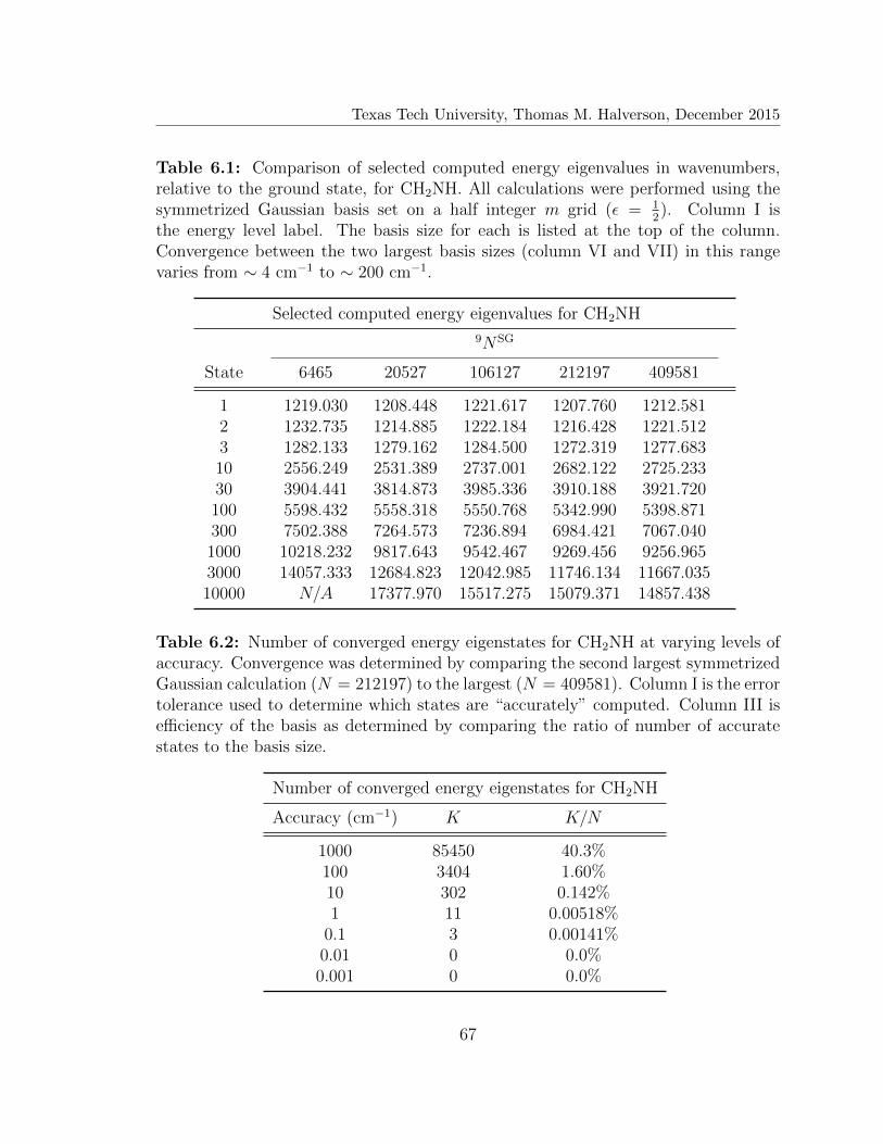
Texas Tech University, Thomas M. Halverson, December 2015
Table 6.1: Comparison of selected computed energy eigenvalues in wavenumbers,relative to the ground state, for CH2NH. All calculations were performed using thesymmetrized Gaussian basis set on a half integer m grid (ε = 1
2). Column I is
the energy level label. The basis size for each is listed at the top of the column.Convergence between the two largest basis sizes (column VI and VII) in this rangevaries from ∼ 4 cm−1 to ∼ 200 cm−1.
Selected computed energy eigenvalues for CH2NH
9NSG
State 6465 20527 106127 212197 409581
1 1219.030 1208.448 1221.617 1207.760 1212.5812 1232.735 1214.885 1222.184 1216.428 1221.5123 1282.133 1279.162 1284.500 1272.319 1277.68310 2556.249 2531.389 2737.001 2682.122 2725.23330 3904.441 3814.873 3985.336 3910.188 3921.720100 5598.432 5558.318 5550.768 5342.990 5398.871300 7502.388 7264.573 7236.894 6984.421 7067.0401000 10218.232 9817.643 9542.467 9269.456 9256.9653000 14057.333 12684.823 12042.985 11746.134 11667.03510000 N/A 17377.970 15517.275 15079.371 14857.438
Table 6.2: Number of converged energy eigenstates for CH2NH at varying levels ofaccuracy. Convergence was determined by comparing the second largest symmetrizedGaussian calculation (N = 212197) to the largest (N = 409581). Column I is the errortolerance used to determine which states are “accurately” computed. Column III isefficiency of the basis as determined by comparing the ratio of number of accuratestates to the basis size.
Number of converged energy eigenstates for CH2NH
Accuracy (cm−1) K K/N
1000 85450 40.3%100 3404 1.60%10 302 0.142%1 11 0.00518%
0.1 3 0.00141%0.01 0 0.0%0.001 0 0.0%
67

Texas Tech University, Thomas M. Halverson, December 2015
What are we to make of these trends, in light of our theorem that (K/N)→ 1 as
N →∞? The only conclusion is that even by N ≈ 200, 000, N is not yet sufficiently
large to achieve this theoretical limit—except for an error tolerance of ∼100 cm−1. In
fact, this is not unexpected; theory predicts that classical PST accounts for about 98%
of the Wigner probability.19–21 It should thus be “easy” to calculate many eigenvalues
to within 2% or so of the energy scale of the problem—which in the present context,
turns out to be ∼ 100 cm−1. Of course, lower energy states are more accurately
computed in the SGB approach—because the corresponding R regions are smaller,
and so R′ incorporates quantum tunneling (outside of the classically allowed region
R) better (See Section 2.2).38 However, the scaling of phase space volume is such
that, for larger D, an increasing fraction of this volume lies in the periphery of the
region—hence making it much more difficult to compute states to the same (higher)
level of accuracy as for smaller D. Though more difficult, the scaling can be shown
to be power law, rather than exponential; nevertheless, in practice, better strategies
than simply increasing N will have to be adopted, if better accuracy is desired (e.g.
HOB hybridization).
68

Texas Tech University, Thomas M. Halverson, December 2015
CHAPTER 7
ACETONITRILE (D = 12)
The work outlined in Chapter 6, which only utilized the SGB, showcases that
on its own a PSLB can be lackluster for systems of increasing D. This is exempli-
fied by the fact that E0 for CH2NH was only converged to a ∼ 400 cm−1. Going
forward, we will need to also utilize both the HOB and the SGB to calculate a more
accurate vibrational spectrum. For the system here (CH3CN), which has dimension-
ality D = 12, we utilized the full power of SwitchBLADE by incorporating three
truncation schemes for HOB—µ = 0.0, µ = 0.5, and µ = 1.0—and the SGB. Based
on the arguments laid out in Chapter 2, we anticipate three distinct spectral regions
over which µ = 0.0, µ = 0.5, and µ = 1.0, in energetically increasing order, are most
accurate (for comparable N)—provided that anharmonicity and mode coupling are
sufficiently small. A maximum energy threshold is also expected, beyond which an-
harmonicity destroys the effectiveness of any HOB truncation scheme, and the SGB
therefore becomes most efficient.
7.1 Force Field Potential
These predictions have been evaluated, using the CH3CN system as a realistically
complex test molecule. Using a D = 12 version of the quartic FFP of Begue and
coworkers,70 we computed the vibrational spectra using the, aforementioned, four
basis sets/truncation schemes. In each case, two different Emax values were considered,
resulting in one “small” (N1) and one “large” (N2) basis set calculation for each, as
indicated in Table 7.1. The Emax values were chosen such that N1 and (to a lesser
extent) N2 are roughly comparable across all four methods.
It should be noted that that the FFP, as described in 70 has too major issues.
The first is that the inconsistency in notation causes ambiguities in the definition of
the coefficients they report (more on that below, also see Chapter 6). The second,
which is slightly more egregious, is that an incomplete number of terms is specified
as to transform the D = 8 reduced coordinate coefficients to a full D = 12 FFP.
The lack of terms leads to ambiguities in how such expansions should be evaluated
according to the Henry and Amat relations.71,72 However, a definite method, based
69

Texas Tech University, Thomas M. Halverson, December 2015
Table 7.1: Basis sizes for each EQD method: smaller (N1) and larger (N2). N isdetermined from Eq. (2.26) for the HOB and Eq. (2.15) for the SGB.
Basis sizes for CH3CN
Method Emax N
µ = 0.0 9.0 12N0.01 = 293930
10.0 12N0.02 = 646646
µ = 0.5 330.5 12N0.51 = 265944
366.2 12N0.52 = 582150
µ = 1.0 10885.0 12N1.01 = 246258
12671.0 12N1.02 = 733313
SGB 0.090 12NSGB1 = 252788
0.092 12NSGB2 = 328224
on how the doubly degenerate normal mode coordinates transform with respect to
the C3v symmetry operations—in particular, the C3 operation—was developed (by
us) that removes these ambiguities.
With regards to the first problem, it can be understood by looking back at
Eq. 2.2, which utilizes a constained summation convention, in that the summation
limits are interdependent. In fact, this is the form that Ref. 71 and 72 requires for
proper expansion. However, the FFP reported in Ref. 70 utilizes unconstrained sums,
where the coefficients are the standard derivative matrix elements,
φijl =∂3V
∂qi∂qj∂ql; φijln =
∂4V
∂qi∂qj∂ql∂qn, (7.1)
and do not contain index permutations. It appears that the φ values, as presented
in Ref. 70 Table 4, might actually be k values. Direct evidence of this can be found
by plotting subsets of the unconstrained CH3CN FFP. We present one such plot
as the dotted curve in Figure 7.1—a 1D reaction profile, expressed in terms of the
coordinate q4 (the C–C stretching mode). The curve exhibits a turnaround “barrier”
near q4 = 7. Such a barrier, per se, is not necessarily problematic, but rather indicates
the onset of dissociation. The problem here is that the unconstrained CH3CN FFP
barrier height is only ∼ 6000 cm−1, whereas the actual C–C bond energy is around
70

Texas Tech University, Thomas M. Halverson, December 2015
Figure 7.1: Reaction profiles for CH3CN, as a function of q4 (C–C stretch). Dottedlines and diamonds represent unconstrained FFP reaction profiles; solid lines andcircles represent constrained FFP reaction profiles.
30,000 cm−1. Alternatively, if the values listed in Ref. 70 Table 4 are interpreted to
be k’s, rather than φ’s, then the resultant constrained CH3CN FFP gives rise to the
much more reasonable reaction profile indicated by the solid curve in Figure 7.1. The
qualitatively different behaviors of the two FFPP’s can be explained by the fact that k
values are generally much larger than their φ counterparts. Consequently, mislabeling
k values as φ values would lead to an (unconstrained) FFP with greatly exaggerated
coupling and anharmonicity—which, in turn, would lead to unreasonably low-lying
turnarounds.
Essentially, this leaves us with two differentD = 8 FFP’s from which to choose. It
turns out that the the choice is quite easy to make since the unconstrained FFP leads
to nonsensical negative eigenenergies when solved using the SGB method, whereas
energy levels computed using HOB are close (within 10 cm−1) to those reported in
Ref. 70. However, agreement should be much stronger if identical FFP’s are utilized.
To this end, we utilized the unconstrained FFP for the HOB calculations and the
constrained FFP for the SGB calculations. This makes hybridization between the
71
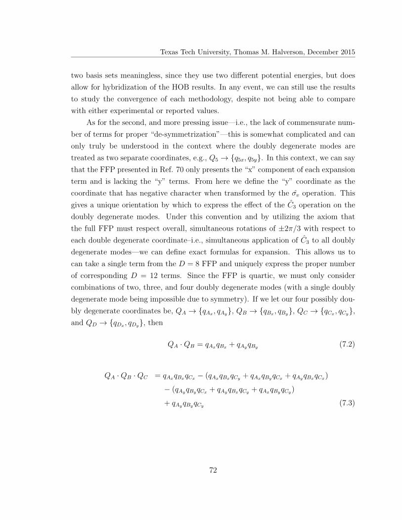
Texas Tech University, Thomas M. Halverson, December 2015
two basis sets meaningless, since they use two different potential energies, but does
allow for hybridization of the HOB results. In any event, we can still use the results
to study the convergence of each methodology, despite not being able to compare
with either experimental or reported values.
As for the second, and more pressing issue—i.e., the lack of commensurate num-
ber of terms for proper “de-symmetrization”—this is somewhat complicated and can
only truly be understood in the context where the doubly degenerate modes are
treated as two separate coordinates, e.g., Q5 → {q5x, q5y}. In this context, we can say
that the FFP presented in Ref. 70 only presents the “x” component of each expansion
term and is lacking the “y” terms. From here we define the “y” coordinate as the
coordinate that has negative character when transformed by the σv operation. This
gives a unique orientation by which to express the effect of the C3 operation on the
doubly degenerate modes. Under this convention and by utilizing the axiom that
the full FFP must respect overall, simultaneous rotations of ±2π/3 with respect to
each double degenerate coordinate–i.e., simultaneous application of C3 to all doubly
degenerate modes—we can define exact formulas for expansion. This allows us to
can take a single term from the D = 8 FFP and uniquely express the proper number
of corresponding D = 12 terms. Since the FFP is quartic, we must only consider
combinations of two, three, and four doubly degenerate modes (with a single doubly
degenerate mode being impossible due to symmetry). If we let our four possibly dou-
bly degenerate coordinates be, QA → {qAx , qAy}, QB → {qBx , qBy}, QC → {qCx , qCy},and QD → {qDx , qDy}, then
QA ·QB = qAxqBx + qAyqBy (7.2)
QA ·QB ·QC = qAxqBxqCx − (qAxqBxqCy + qAxqByqCx + qAyqBxqCx)
− (qAyqByqCx + qAyqBxqCy + qAxqByqCy)
+ qAyqByqCy (7.3)
72

Texas Tech University, Thomas M. Halverson, December 2015
QA ·QB ·QC ·QD = qAxqBxqCxqDx +1
3(qAxqBxqCyqDy
+ qAxqByqCxqDy + qAyqBxqCxqDy
+ qAxqByqCyqDx + qAyqBxqCyqDx
+ qAyqByqCxqDx) + qAyqByqCyqDy , (7.4)
with all non-degenerate modes having a 1-to-1 correspondences to the terms in the
D = 12 FFP. These three equations allow us to take any D = 8 coefficient and
uniquely define either two or eight corresponding D = 12 terms, mapping the the
reduced coordinate space to the full coordinate space.
7.2 Results
Once we properly calculated the full FFP, we computed vibrational eigenstates
using all four methods. To help reduce the computation time, and allow access to
large N values, the HOB calculations were split based on the σv operation, which,
again, yields negative character for the “y” components of the doubly degenerate
coordinates. This created two separate blocks—one with A ⊕ Ex character and one
with B ⊕ Ey. It should be noted that this was not an option for the SGB since the
underlying functions do not have the same even/odd parity. After all the calcula-
tions were completed and the blocks recombined using energetic ordering, the HOB
calculations were also hybridized—i.e., the eigenstates from three different trunca-
tion methods were combined into a new data set (see Section 2.4). Again, the idea
is straightforward: since all calculations are variational, the lowest-lying computed
energy eigenvalue at a given point in the spectrum is the most accurate. One way
to judge the validity of the HT dataset is to investigate E0 for each calculation. We
see that for µ = 0.0, which is expected to yield the most converged eigenenergies
at the bottom of the spectrum, E0 varies by only 0.0002 cm−1 from small to large.
This gives good indication that overall spectrum is not only well converged, but also
accurate. Moreover, E0 for µ = 1.0, which is expected to do poorest for low energies,
is converged to 0.53 cm−1 and only differs is actual value from µ = 0.0 by 1.96 cm−1.
In general, the lack of variation, method-to-method, of E0, combined with the spec-
troscopic convergence of µ = 0.0 leads us to believe that a hybrid spectrum will not
73
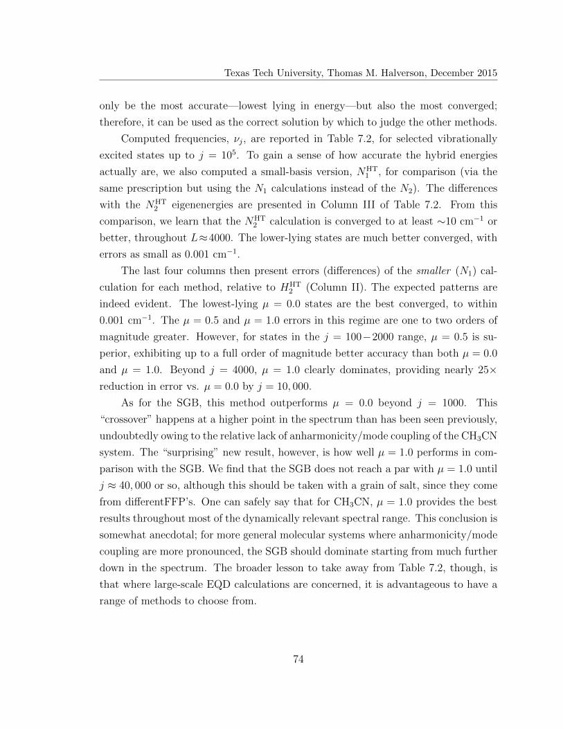
Texas Tech University, Thomas M. Halverson, December 2015
only be the most accurate—lowest lying in energy—but also the most converged;
therefore, it can be used as the correct solution by which to judge the other methods.
Computed frequencies, νj, are reported in Table 7.2, for selected vibrationally
excited states up to j = 105. To gain a sense of how accurate the hybrid energies
actually are, we also computed a small-basis version, NHT1 , for comparison (via the
same prescription but using the N1 calculations instead of the N2). The differences
with the NHT2 eigenenergies are presented in Column III of Table 7.2. From this
comparison, we learn that the NHT2 calculation is converged to at least ∼10 cm−1 or
better, throughout L≈4000. The lower-lying states are much better converged, with
errors as small as 0.001 cm−1.
The last four columns then present errors (differences) of the smaller (N1) cal-
culation for each method, relative to HHT2 (Column II). The expected patterns are
indeed evident. The lowest-lying µ = 0.0 states are the best converged, to within
0.001 cm−1. The µ = 0.5 and µ = 1.0 errors in this regime are one to two orders of
magnitude greater. However, for states in the j = 100−2000 range, µ = 0.5 is su-
perior, exhibiting up to a full order of magnitude better accuracy than both µ = 0.0
and µ = 1.0. Beyond j = 4000, µ = 1.0 clearly dominates, providing nearly 25×reduction in error vs. µ = 0.0 by j = 10, 000.
As for the SGB, this method outperforms µ = 0.0 beyond j = 1000. This
“crossover” happens at a higher point in the spectrum than has been seen previously,
undoubtedly owing to the relative lack of anharmonicity/mode coupling of the CH3CN
system. The “surprising” new result, however, is how well µ = 1.0 performs in com-
parison with the SGB. We find that the SGB does not reach a par with µ = 1.0 until
j ≈ 40, 000 or so, although this should be taken with a grain of salt, since they come
from differentFFP’s. One can safely say that for CH3CN, µ = 1.0 provides the best
results throughout most of the dynamically relevant spectral range. This conclusion is
somewhat anecdotal; for more general molecular systems where anharmonicity/mode
coupling are more pronounced, the SGB should dominate starting from much further
down in the spectrum. The broader lesson to take away from Table 7.2, though, is
that where large-scale EQD calculations are concerned, it is advantageous to have a
range of methods to choose from.
74
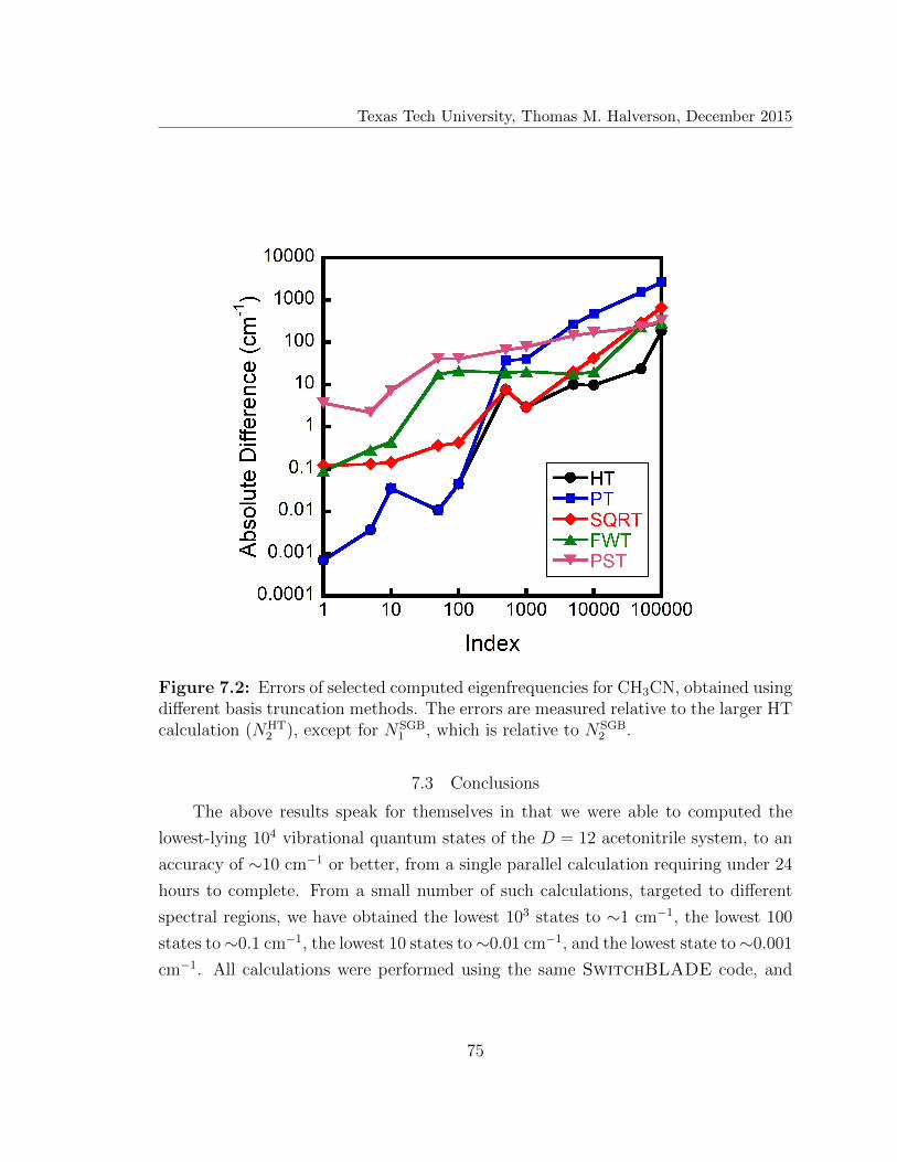
Texas Tech University, Thomas M. Halverson, December 2015
Figure 7.2: Errors of selected computed eigenfrequencies for CH3CN, obtained usingdifferent basis truncation methods. The errors are measured relative to the larger HTcalculation (NHT
2 ), except for NSGB1 , which is relative to NSGB
2 .
7.3 Conclusions
The above results speak for themselves in that we were able to computed the
lowest-lying 104 vibrational quantum states of the D = 12 acetonitrile system, to an
accuracy of ∼10 cm−1 or better, from a single parallel calculation requiring under 24
hours to complete. From a small number of such calculations, targeted to different
spectral regions, we have obtained the lowest 103 states to ∼1 cm−1, the lowest 100
states to∼0.1 cm−1, the lowest 10 states to∼0.01 cm−1, and the lowest state to∼0.001
cm−1. All calculations were performed using the same SwitchBLADE code, and
75

Texas Tech University, Thomas M. Halverson, December 2015
the parallel computing cluster employed—though large—is much less massive than
certain newer machines, on which a single job can access more than 105 cores.
Massive parallelization alone has not made this possible—though it certainly
plays a critical and increasingly important role in EQD advancement. Rather, the
most important contributor is the classical PSP, serving as a useful and versatile—
perhaps even indispensable—tool for basis set optimization of large-D systems. Such
applications are simply too large and complex to be optimized successfully via trial
and error—at least not in any straightforward “black-box” fashion suitable for non-
expert users. As a case in point, m = 0.0 truncation has been used for many years,
essentially without a solid understanding that this approach is optimized only for
the very bottom of the spectrum—or at least, of why that is the case. The PSP not
only provides such an understanding, but also points to a different truncation scheme
which, provides ∼25× better performance, in the much more challenging high-lying
part of the dynamically relevant spectrum. More generally, the PSP serves as both
a rigorous and practical criterion—for large dimensional systems, perhaps the only
such—for assessing a priori the efficiency of an arbitrary basis set. This feature
could have very important ramifications for existing methodologies and codes that
are already widely used.
The PSP also provides a clear and quantitative understanding of exponential
scaling: both where it comes from, and how to eradicate it (See Chapter 2). It has
been used both to develop the SGB method—which defeats exponential scaling—as
well as to understand its limitations. Likewise, we have used it here to both optimize
and analyze the correlated truncation of DPB’s, as has not been done previously to
our knowledge. It seems likely that this versatile workhorse will become increasingly
relied upon for the future advancement of EQD methodologies and applications.
That said, some major challenges are also anticipated. Regarding massive par-
allelization, modern architectures are idiosyncratic, leading to unpredictable and
platform-specific performance vis-a-vis scalability. It seems that hierarchical caching
structures, multi-core CPU’s, proprietary interconnects, combined shared- and distributed-
memory computing, etc., have all conspired to usher in a new era of computing not
entirely dissimilar to the early days of mainframes and assembly languages. In any
76
Texas Tech University, Thomas M. Halverson, December 2015
event, such technical and practical concerns will increasingly have to be accounted for
if EQD calculations are to take full advantage of parallel architectures going forward.
Regarding methodology, both HOB truncation and SGB have their drawbacks.
According to the phase space picture, however, these are quite complementary. Thus,
the former approach is well adapted to the lower-lying spectrum, whereas the latter
is better suited to higher spectral regions, where coupling and anharmonicity are
more pronounced. In that respect, the SGB is more versatile than the HOB, and will
soon be applied to systems with “floppy” or multi-well PES’s (although the Switch-
BLADE code is still currently limited to FFP’s). Nevertheless, from a practical
standpoint, both methods are necessary for tackling general problems; accordingly,
both are implemented in SwitchBLADE. Ultimately, though, the PSP may inspire
a single method with the best features of both.
77
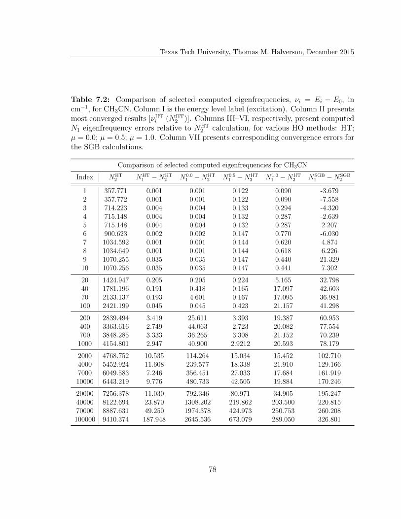
Texas Tech University, Thomas M. Halverson, December 2015
Table 7.2: Comparison of selected computed eigenfrequencies, νi = Ei − E0, incm−1, for CH3CN. Column I is the energy level label (excitation). Column II presentsmost converged results [νHT
i (NHT2 )]. Columns III–VI, respectively, present computed
N1 eigenfrequency errors relative to NHT2 calculation, for various HO methods: HT;
µ = 0.0; µ = 0.5; µ = 1.0. Column VII presents corresponding convergence errors forthe SGB calculations.
Comparison of selected computed eigenfrequencies for CH3CN
Index NHT2 NHT
1 −NHT2 N0.0
1 −NHT2 N0.5
1 −NHT2 N1.0
1 −NHT2 NSGB
1 −NSGB2
1 357.771 0.001 0.001 0.122 0.090 -3.6792 357.772 0.001 0.001 0.122 0.090 -7.5583 714.223 0.004 0.004 0.133 0.294 -4.3204 715.148 0.004 0.004 0.132 0.287 -2.6395 715.148 0.004 0.004 0.132 0.287 2.2076 900.623 0.002 0.002 0.147 0.770 -6.0307 1034.592 0.001 0.001 0.144 0.620 4.8748 1034.649 0.001 0.001 0.144 0.618 6.2269 1070.255 0.035 0.035 0.147 0.440 21.32910 1070.256 0.035 0.035 0.147 0.441 7.302
20 1424.947 0.205 0.205 0.224 5.165 32.79840 1781.196 0.191 0.418 0.165 17.097 42.60370 2133.137 0.193 4.601 0.167 17.095 36.981100 2421.199 0.045 0.045 0.423 21.157 41.298
200 2839.494 3.419 25.611 3.393 19.387 60.953400 3363.616 2.749 44.063 2.723 20.082 77.554700 3848.285 3.333 36.265 3.308 21.152 70.2391000 4154.801 2.947 40.900 2.9212 20.593 78.179
2000 4768.752 10.535 114.264 15.034 15.452 102.7104000 5452.924 11.608 239.577 18.338 21.910 129.1667000 6049.583 7.246 356.451 27.033 17.684 161.91910000 6443.219 9.776 480.733 42.505 19.884 170.246
20000 7256.378 11.030 792.346 80.971 34.905 195.24740000 8122.694 23.870 1308.202 219.862 203.500 220.81570000 8887.631 49.250 1974.378 424.973 250.753 260.208100000 9410.374 187.948 2645.536 673.079 289.050 326.801
78

Texas Tech University, Thomas M. Halverson, December 2015
CHAPTER 8
BENZENE (D = 30)
Benzene represents the culmination of the power of SwitchBLADE. In fact,
many of the calculations contained herein are some of the largest direct matrix di-
aganolizations that have been done to date (at least for the purpose of real calcu-
lations). The PES used for benzene is a full D = 30 FFP, developed by N. Handy
and coworkers. They used ab initio self-consistent field calculations, with double-zeta
plus polarization basis sets, to compute all quadratic, cubic and quartic force con-
stants, omitting coefficients < 1.0 cm−1. They then used Spectro73,74 to compute
anharmonic frequencies, νtheoryj , via second-order PertT. After comparing with exper-
imental values, νexptj (although benzene has only four infrared-active modes),75 they
discovered substantial disagreement, with |νexptj − νtheory
j | > 100 cm−1 in some cases.
To partially correct for this, they defined a new FFP for which all of the new harmonic
frequencies were adjusted via ωj → ωj + νexptj − νtheory
j (Table 8.1). Finally, they used
Spectro to recompute the anharmonic frequencies, together with a few combination
bands. Due to the accuracy limitations of second-order PertT—and the rather large
magnitude of the semi-empirical corrections employed—it is not expected that the
more accurate spectroscopic calculations conducted here will yield better agreement
with experiment. Nevertheless, this FFP serves as a very realistic and challenging
benchmark application for our PSP methods.
The reduced normal mode coefficients as presented in Ref. 76 can be expanded
to the full D = 30 FFP using the Henry and Amat symmetry relations.71,72 It should
be noted that Ref. 76 contains the correct number of reduced coordinate coefficient
values needed to properly expand the full FFP, save one. The term, Φ16a16a6a6a is not
reported, even though its symmetry partner, Φ16a16a6b6b , is reported. To be on the
safe side, and since the numerical value of the reported Φ16a16a6b6b coefficient is only
2.9 cm−1, we simply ignore both terms. Because the numerical value is small, it should
not play a large role in the overall coupling, but it is difficult to make exact claims
into how much of a role this could play at very high excitation. The major downside
of not having a proper explanation of how this term was handled by the original
author is that it makes direct comparison to the calculated frequencies somewhat
79

Texas Tech University, Thomas M. Halverson, December 2015
Table 8.1: Adjusted normal mode harmonic frequencies, ωj, as used in the quar-tic FFP developed by N. Handy and coworkers.76 Column I: full D = 30 normalmode labels, for which each doubly degenerate mode receives two labels. ColumnII: “reduced” (D = 20) normal mode labels, for which each doubly degenerate modereceives a single label.
Normal mode frequencies for C6H6
Mode
j Reduced D6h irrep ωk (cm−1)
1 1 A1g 10082 2 A1g 32083 3 A2g 13904 4 B2g 7185 5 B2g 1011
6,7 6 E2g 6138,9 7 E2g 3191
10,11 8 E2g 163912,13 9 E2g 119214,15 10 E1g 866
16 11 A2u 68617 12 B1u 102418 13 B1u 317219 14 B2u 131820 15 B2u 1167
21,22 16 E2u 40723,24 17 E2u 98925,26 18 E1u 105827,29 19 E1u 151229,30 20 E1u 3191
spurious, but since the methods used for those calculations are somewhat older, and
approximate, the small potential difference will most likely not be the limiting factor
in the difference between the computed states presented here and those in the original
paper. In any event, direct comparison to the aforementioned results is not the focus,
like was the case with previous systems, and this difference in no way affects the
convergence and accuracy of the results presented.
80
Texas Tech University, Thomas M. Halverson, December 2015
For the D = 30 benzene application, symmetry adaptation of the basis set is
required in order to reduce the basis size N to a tractable size, even for a massively
parallel computer. Benzene belongs to the D6h point group, which has 8 singly- and
4 doubly-degenerate irreducible representations (irreps). Unfortunately, the HOB
representation does not respect the full D6h symmetry of the problem. However, the
HOB functions transform very straightforwardly (with ±1 character) under each of
the three commuting symmetry operations, i, σv, and C2. This property is easily
exploited to allow for an 8–fold reduction in N (eight independent symmetry blocks),
reducing the largest basis size from N = 5, 706, 342 down to N = 719, 588. Direct
diagonalization for matrices of even this size are quite challenging, requiring wall
times of ∼ 40 hrs. despite being run in parallel across 7200 cores. The large N
values needed, and the fact that HOB respects some of the system symmetry and
the SGB does not, meant there was no reason to utilize the SGB for a full spectral
analysis because the N values would be too small as to affect the hybrid calculation.
Therefore, only HOB’s were utilized.
Three sets of calculations were done using the benzene FFP, corresponding to
three different µ values: µ = 0.1; µ = 0.5; µ = 1.0. For each µ value, calculations for
three different N ’s were conducted: small; medium; large. One such calculation was
performed for each of the eight symmetry blocks, resulting in a total of 72 separate
calculations in all. The normal mode frequencies, ωk, used in Eq. (2.26), are the
adjusted benzene frequencies as presented in Ref. 76 and also Table 8.1.
As discussed, Emax values were chosen so that small, medium, and large basis
sizes, NµEmax
, are comparable across µ. The resultant basis sizes as used in each of the
72 calculations can be seen in Table 8.2, along with the irrep decomposition of each
symmetry block. Specifically, each symmetry block corresponds to a unique singly-
degenerate irrep (eight in all), plus one half of a corresponding doubly degenerate
irrep (four in all). The splitting of the doubly-degenerate modes across two blocks
(chosen to be adjacent odd-even rows in the table) makes it possible to uniquely iden-
tify the D6h irrep for any given state, by comparing computed energy levels across
the block pair. For all of the analysis presented here, eigenvalues are only compared
block to block to ensure that we are comparing states with the same symmetry. This
ensures that psuedo-convergence does not cause two states, with different symmetry,
81

Texas Tech University, Thomas M. Halverson, December 2015
Table 8.2: Basis sizes, NµEmax
, as truncated in accord with Eq. (2.26), using threedifferent Emax values for each of three different truncation schemes, µ. The Emax
values were adjusted in such a way as to ensure that small, medium, and large NµEmax
values are roughly constant across µ.
Basis Sizes for C6H6
Symmetry µ = 0.1 µ = 0.5 µ = 1.0
Block D6h irreps 30N0.113.28
30N0.113.88
30N0.114.23
30N0.5215.0
30N0.5223.0
30N0.5237.0
30N1.06600.0
30N1.06800.0
30N1.07278.0
1 A1g ⊕ E2gx 250063 372485 719588 245756 364971 716302 259479 351713 7162052 A2g ⊕ E2gy 248580 370870 717697 244591 363543 714140 258156 350166 7139193 B1u ⊕ E1ux 248947 371390 717955 244617 363467 714052 257997 349825 7120084 B2u ⊕ E1uy 248584 371054 717602 244411 363206 713560 257692 349458 7114285 B1g ⊕ E1gx 239179 361028 707327 242506 361022 709793 257050 349274 7108106 B2g ⊕ E1gy 239881 362210 709084 243423 362203 711467 258023 350428 7125527 A1u ⊕ E2ux 239505 361787 708032 243275 361808 711087 258024 349979 7135498 A2u ⊕ E2uy 239897 362491 709057 243774 362491 712037 258582 350637 714547
total — 1954636 2933315 5706342 1952353 2902771 5702438 2065003 2801480 5705018
to swap positions in the indexing scheme. All estimates of numerical convergence
are accomplished by calculating differences between the large N calculation, and the
corresponding medium or small N calculation. This provides two separate conver-
gence estimates for each eigenstate. The presentation of two such convergence values
allows for a better understanding of convergence, and also helps to rule out spurious
or pseudo-convergence.
8.1 Low-lying energy levels
For the lowest lying 30+ states in each symmetry block (257 total), we used
energetic ordering of the ωj, together with symmetry considerations, to assign state
labels based on mode excitations. The symmetry characters for the overtone and
combination states were determined using the D6h product table. This procedure is
straightforward—except that care must be taken to exclude antisymmetric combina-
tions when there are multiple excitations of the same doubly degenerate mode. For
example, two excitations of ω16, which has E1g character, should yield four states
since E2g ⊗ E2g = A1g ⊕ A2g ⊕ E2g. However, the A2g state, which results from the
antisymmetric combination of the modes, is a virtual state—i.e., the antisymmetric
linear combination of the double degenerate mode coordinate is equal to zero since it
is a combination of the same mode, qxqy − qxqy = 0. In fact, this is true regardless
82
Texas Tech University, Thomas M. Halverson, December 2015
of whether the character is gerade or ungerade. Excluding these forbidden combina-
tions, we deduce the following combination rules for multiple products of identical
doubly-degenerate modes:
E ⊗ E = A1 ⊕ E1
E1 ⊗ E1 ⊗ E1 = B1 ⊕B2 ⊕ E1
E2 ⊗ E2 ⊗ E2 = A1 ⊕ A2 ⊕ E1
E ⊗ E ⊗ E ⊗ E = A1 ⊕ E1 ⊕ E1. (8.1)
Note that the 1 and 2 subscripts do not play a roll in even-power products, but do
do so when the power is odd.
The low-lying states as described above are presented in Tables 8.3–8.10, for
which one table corresponds to each symmetry block. State labels are pre-
sented in Column II, in “reduced” (D = 20) normal mode notation [e.g., (6, 7) → 6,
(8, 9) → 7, etc.; see Table 8.1]. The corresponding frequencies, νi = Ei − E0, are
presented in Column V. Since µ = 0.1 is expected to be most accurate at the bot-
tom of the spectrum, the frequencies correspond to the large µ = 0.1 calculation—i.e.,
N0.114.23. Columns VI and VII present ∆νi = νi−ν large
i —i.e., the numerical convergence
of the medium and small calculation frequencies, respectively, relative to the large
calculation. About half of the frequencies are converged to subwavenumber accuracy,
with the rest converged to within just a few cm−1’s. However, ν’s that result from a
large excitation of a single low-frequency mode tend to be less well converged. This
is inline with the analysis presented in Section 2.4, since µ = 0.1 treats all modes
equally. For example, 4v16 (Table 8.3) displays particularly poor convergence despite
being a relatively low energy mode. The cause of this could go beyond the number
of excitations, and could be resultant from a large amount of anharmonicity in that
particular mode, or some large amount of coupling to another mode, but finding the
exact cause would prove quite difficult due to the large dimensionality of the space.
Along with the states computed using SwitchBLADE, Tables 8.3–8.10 also
show ν’s from Ref. 76 (where available) obtained using second-order PertT, in Col-
umn IV. Since identical FFP’s were employed here as in Ref. 76, a direct comparison
of Columns IV and V provides an estimate of the error associated with second-order
83
Texas Tech University, Thomas M. Halverson, December 2015
PertT. These errors are generally on the order of 10 cm−1’s, although in some cases
they are significantly larger. In some of the cases the reference v’s are lower in value
compared to our calculations. However, the lack of approximation used by Switch-
BLADE leads us to conclude that our calculations are more accurate, and there is
some amount of anhamarmonicity that their approximation is not taking into account.
That is not to say there are any large discrepancies between our calculated states and
those from Ref. 76. In fact, the difference is never more that a few wavenumbers.
In any event, we report many more energy levels than in Ref. 76, as the latter au-
thors were primarily concerned with just those states for which experimental data is
available, mainly because they are only concerned with mode that are E1 active. It
should be noted that in the cases where we can compare, our error is smaller than
the difference between their approximate calculation and our direct calculation, e.g.
v4 + v16 where our calculated frequency differs from the reference value by ∼ 3 cm−1
but is converged to ∼ 0.2 cm−1.
8.2 High-lying energy levels
Reporting and properly assigning the low-lying ν’s is important, but the true
power of the PSP approach is not realized until we consider more highly-excited
states. For a large molecule such as benzene, the L is quite large, L > 105. Table 8.11
presents frequencies for a selection of dynamically relevant excited states, i, ranging
from i = 1 to i = 106, across all eight symmetry blocks (Column I). To generate this
table, the computed energy levels from all blocks were first concatenated together, and
then resorted by energy. Columns II, V, and VIII, list frequencies, νi, as computed
using the large calculation for each of the three truncations, µ = 0.1, µ = 0.5, and
µ = 1.0, respectively. The corresponding E0’s are 217866.6 cm−1, 21790.8 cm−1, and
21850.7 cm−1. The remaining columns indicate numerical convergence, of the three
medium and small calculations, relative to the corresponding large calculations. Note
that here we present convergence of the energy levels—i.e., ∆Ei = Ei−Elargei —rather
than the frequencies. The third row in the table indicates which basis set was used
for each calculation, using NµEmax
notation.
Table 8.11 also serves to show how each truncation method performs, in different
regions of the spectrum. We find that the numerical convergence patterns are not as
84

Texas Tech University, Thomas M. Halverson, December 2015
“clean” as anticipated in Chapter 2—nor indeed, as was observed in Chapter 7. To be
sure, µ = 1.0 is least well converged near the bottom of the spectrum, and the small
µ = 0.1 calculation is very poorly converged as i→ 106, in accord with expectation.
On the other hand, the medium µ = 0.1 calculation appears the most converged
near the top of the spectrum. In reality, this is most likely a pseudo-convergence,
owing to the (nearly)-perfectly-symmetric PT behavior discussed in Section 2.4. It
might also be due to the limited range of the N values considered; even though the
large-to-small basis ratio used here is nearly 3×, which is quite large, it may be that
for D≈30, even larger ratios are needed. In any event, one solid indication that this
is a pseudo-convergence, besides the fact that the small µ = 0.1 errors are so large,
is the fact that the computed frequency, e.g. for i = 106, is several hundred cm−1’s
larger than for either of the other two µ values.
We must be a bit careful in comparing frequencies rather than energy levels across
methods, as only the latter are variational. Thus, the fact that µ = 1.0 provides the
smallest ν1 value should not be taken as an indication that this is the most accurate
frequency value, but rather, that it corresponds to the least well converged ground
state. That said, a “lowest” frequency comparison is legitimate for differences that are
greater than the worst convergence of the ground state energy—in this case, around
2.5 cm−1’s. By this reckoning, one sees that µ = 0.1 is indeed least accurate at the
highest energies.
With one million states to choose from, it might in principle be the case that the
small sampling considered in Table 8.11 happens not to be representative. We there-
fore next turn our attention to statistics gathered across all 106 states. Tables 8.12–
8.14 indicate the total numbers of energy levels that are converged to within different
error tolerances, for the µ = 0.1, µ = 0.5, and µ = 1.0 calculations, respectively.
We see the same basic patterns as described above. For example, µ = 0.1 yields 318
states that are converged to within 4 cm−1, whereas µ = 1.0 yields only one such
state. Conversely, µ = 1.0 yields 652,066 levels to within 15 cm−1—i.e., nearly 2/3
of the desired 106 states—whereas µ = 0.1 yields only 33,233 such states. Although
this is in keeping with the expected pattern, in actuality the latter number should
probably be even smaller, owing to the aforementioned pseudo-convergence.
85
Texas Tech University, Thomas M. Halverson, December 2015
Up to now, we have made very little mention of µ = 0.5. This is because it
does not seem to behave in the manner in which we would expect. According to to
the analysis outlined Section 2.4, we would expect there to be some middle range in
which µ = 0.5 outperforms µ = 0.1. If we compare Table 8.12 and Table 8.13 we see
this is not the case. In fact, there is no level of convergence in which µ = 0.5 is better
than µ = 0.1. However, this is only true if viewed in the context of “convergence”—
i.e., µ = 0.5 does not have any range where the difference between the eigenstates
calculated using the larges N and the smaller N is overall smaller than µ = 0.1. This
is actually very apparent in Table 8.11, where for the most part no single method
shines in terms of error. That is not to say that µ = 0.5 is an unnecessary calculation.
On the the contrary, if we view the three methods in terms of their overall eigenenergy
values, µ = 0.5 has a lower eigenspectrum throughout the “middle range” of energies
(m ≈ 103 − 104). From a variational standpoint, µ = 0.5 is more “accurate” in
that range because the calculate eigenvalues are lower in energy that either of the
other three methods. The reason this is not apparent in Table 8.11 or Tables 8.12-
8.14 is because E0 varies quite differently between the three methods. In our work
with acetonitrile, we were able to converge E0 to subwavenumber between the three
methods. Here, E0 differs by up to 64 cm−1 between the largest µ = 0.1 and µ = 1.0
calculations. More interestingly, between the three calculations done via each method,
E0 only varies by 0.1 cm−1 for µ = 0.1 and µ = 1.0, whereas E0 drops by 0.1 cm−1
from the smallest to the largest N values for µ = 0.5. This leads one to believe
that the efficiency cliff described in Chapter 4 may be responsible for the psuedo-
convergence displayed by µ = 0.1 and µ = 1.0. However, the nature of how these
types of calculations converge ensures that the frequency spectrum, relative to E0, is
similar despite the difference in E0 between each method, as can be seen in Table 8.11,
where the first frequency only varies by a few wavenumbers method to method.
8.3 Hybrid Truncation (HT) dataset
All of the above serves to indicate that where large D and K energy level cal-
culations are concerned, we should:(a) take care when interpreting convergence and
accuracy; (b) rely on a range of different truncation methods. Both of these ideas
come together in the HT procedure of Section 2.4, which also introduces a third cru-
86
Texas Tech University, Thomas M. Halverson, December 2015
cially important element: the variational principle. Because the variational principle
enables us to rigorously compare energy levels across truncation methods, it pro-
vides the unambiguously most accurate results, while at the same time mitigating
the vagaries that individual truncation methods might exhibit at one point or an-
other throughout the spectrum (such as pseudo-convergence). Moreover, with regard
to individual calculations, “the more the merrier”; with HT, it can never hurt to add
new calculations into the mix, even if they are not very accurate.
In the present context, for instance, based on the discussion in the previous sec-
tion, one might be tempted to exclude the µ = 0.5 calculations from the hybridization.
In reality though, not only does it not hurt to do so, it actually helps very substan-
tially. Indeed, hybridization is the most rigorous procedure for determining which
method is most useful where—because it does not depend on a convergence compar-
ison between basis sets of two (substantially) different sizes. Table 8.15 shows the
number of states that contribute to the HT dataset, as culled from the large calcu-
lations for each of the three truncation methods (throwing in the small and medium
calculations would not change anything).
Here, we see a very clear pattern in accord with expectation: the fewest and
presumably mostly lowest-lying states, about 15,000 in all, come from µ = 0.1; an
intermediate number, about 400,000, come from µ = 0.5; the vast majority, around
5.3× 10⁶, come from µ = 1.0. As also indicated in the table, the relative percentages
are reliably consistent even across symmetry blocks.
Table 8.16, Column III presents frequencies, νi, for selected eigenstates i, as
taken from the HT dataset. Note that these represent the most accurate benzene
frequencies presented in this paper. In Columns IV and V, we present energy level
convergence errors, ∆EHTi , for the medium and small calculations of the same µ
value as that from which the given HT state i came from (indicated in Column II).
Defined in this fashion, the HT convergence errors for individual states are the same
as those for the constituent truncation methods, and so we do not necessarily observe
an enormous reduction. The full advantage of HT may not be completely evident
in the convergence data, but it is nevertheless very substantial. This is because HT
optimizes for accuracy rather than convergence. In any event, Table 8.17 offers a
more complete picture of HT convergence, by providing statistical data across all 106
87

Texas Tech University, Thomas M. Halverson, December 2015
states, in the same format as Tables 8.12–8.14. From this data we see that by utilizing
HT we get almost the same number of ∆E = 4 states, 316, that we saw with µ = 0.1
while still retain a very high number of ∆E = 15 states, 19% of the total spectrum.
Remarkably, we even see that 66% of the spectrum is converged to below 40 cm−1.
That is a almost 2 million states, easily reaching our sought after goal of the full
dynamically relevant range. However, tens of wavenumbers is not spectroscopic, and
in a perfect world we would seek to go beyond that. Going larger would hopefully
push the efficiency cliff down to the ∆E = 4 level or beyond, but calculations at
this level are still quite usefully for calculating dynamically relevant quantities, e.g.
partition functions, despite the states not being considered super converged.
8.4 Conclusions
By combining phase space ideas with massive parallelization, we have computed
all one million of the dynamically relevant vibrational quantum states for the 12-
atom benzene molecule, to a converged accuracy of ∼10−1–101 cm−1. Moreover, with
respect to the most accurate frequencies as presented in Table 8.16 Column III, we
have done so using only 24 calculations in all. Such a feat—i.e., combining large D
with very large K in an EQD context—would have been unheard of just a few years
ago. Yet, despite the advanced computer hardware used, it is the PSP approach itself
that has primarily made this possible.
No developments in hardware alone can overcome the EQD exponential scaling
problem. In contrast, PSP ideas are what have led to the creation of the only EQD
methods (PSLB) formally known to circumvent exponential scaling.19–21 Here, we
have extended the utility of PSP ideas still further, by using them to develop an HOB
truncation scheme that is not only customized for individual molecular systems, but
also tailored for specific regions of the energetic spectrum. Also, we have learned
from this study that large D—and more so very large K—calculations can benefit
from a range of different EQD calculations. When combined with the variational
principle, this enables the construction of a hybrid dataset that is not only optimally
accurate throughout the entire spectral range, but also exhibits more stable numerical
convergence.
88
Texas Tech University, Thomas M. Halverson, December 2015
The PSP is so useful because it provides simple, clear, intuitive insight, offering
answers to a broad range of potential questions. Over the years, it has been used to
optimize DVR’s,5,28 explain exponential scaling,38and overcome it.18–21 It not only
offers optimal EQD basis set representations, it also provides powerful a priori tools
for estimating (and improving) their accuracy and convergence scaling. We anticipate
that PSP ideas will continue to provide useful insight in new and unanticipated ways—
particularly for large D, very large K applications of the sort considered here.
For the present benzene study, we have chosen to use massively parallel comput-
ers because such resources are available to us—and because these will be the tools of
cutting edge computational science, going forward. Also, massively parallel calcula-
tions provide many eigenvalues at once. So for large molecules, for which there are
a great many dynamically relevant quantum states, such calculations are extremely
convenient. However, it is more than just this. We have also learned that the con-
vergence of PSP HOB exhibits a pronounced efficiency cliff. This means that a small
increase in basis size can lead to a dramatic increase in the number of states converged
to a given accuracy level—creating a strong impetus to work with as large a basis
size, N , as possible.
Also with this study, one of our goals was to push the limits of our present, simple
SwitchBLADE codes as far as possible. Thus, we sought the largest D and N values
for which we could feasibly perform direct diagonalization on a massively parallel
computer. That is not to say that our PSP methods require such specialized hardware,
however. On the contrary, for somewhat smaller but still highly challenging systems,
hundreds or thousands of dynamically relevant states can be computed utilizing much
more modest computational resources.
Alternatively, since the Hamiltonian matrix (and even its symmetry blocks) are
sparse, it is also possible to combine PSP HOB truncation with iterative methods—
thereby extending the realm of applicability of the latter, while simultaneously ren-
dering benzene-like calculations possible on much smaller computing clusters than
those employed here. Also, one could then tackle substantially larger basis sizes,
N . This is an area of future investigation. As discussed in Chapter 1, however, the
downside to the iterative approach is that relatively few states can be computed at a
time.
89

Texas Tech University, Thomas M. Halverson, December 2015
Whether iterative or direct eigensolvers are employed, one current drawback of
the PSP methods that must be addressed going forward is the accuracy limitation: for
large D, one can evidently attain high convergence accuracy or very high efficiency,
(K/N), but not both at the same time. Finding ways to simultaneously improve both
is therefore an ongoing area of investigation. In particular, early work done by our
group resulted in a methodology for dramatically increasing the accuracy of PSLB’s
without compromising efficiency.13,14,22 This method (PSRO, see Chapter 4) not only
increase efficiency—i.e., less basis functions are needed for decent convergence—but
also increased the amount of convergence. Under normal circumstances, calculations
done via PSLB would be combined with those from a HOB in order to further optimize
the hybrid process. However, in the case of benzene the lack of symmetry of PSLB
does not allow for any reduction in the size of the calculations. This makes accessing
the N values for which PSLB states are reasonably converged extremely difficult.
However, by utilizing PSRO’s we could compute a PSLB spectrum that is converged
enough to be useful in HT, despite not being able to access very large basis sizes. Also,
by implementing PSRO’s into SwitchBLADE we might be able obviate HOB’s
entirely, if the increased efficiency bypassed that of HOB’s. Most likely, PSRO’s
could not push passed µ = 0.0 HOB, but it could easily be the case that they perform
better than mu = 1.0 HOB. In any event, as was stated before, the beauty of HT
is that we do not lose anything by introducing more types of truncation. However,
it should be noted that the study in Ref. 22 only looked at model applications up
to D = 4, but the results proved extremely encouraging. All in all, many challenges
for a large D, very large K implementation still remain—particular vis-a-vis massive
parallelization.
Another, slightly less pressing issue going forward is the generalization for ar-
bitrary (i.e., non-FFP) PES’s. Currently, the SwitchBLADE codes are restricted
to quartic FFP’s—although this does not reflect an inherent limitation of the un-
derlying PSP methods themselves. For PSP HOB’s, in particular, Gauss-Hermite
quadrature77 is a natural tool for representing arbitrary PES’s; moreover, a similar
approach has been developed for PSLB’s, in a manner that itself avoids exponential
scaling.51 To date, we have not implemented these techniques into SwitchBLADE,
primarily for two reasons. First, for D ≈ 15–30, there are very few non-FFP PES’s
90
Texas Tech University, Thomas M. Halverson, December 2015
in existence. Second, the accuracy limitation of most FFP PES’s is on the order of
tens of cm−1’s—i.e., comparable to the worst convergence error that SwitchBLADE
currently provides. As PES quality and PSP accuracy improve, however, the moti-
vation for doing so will increase. We also note, though, that the introduction of
quadrature removes the rigorously variational property that is so beneficial for the
HT procedure—although how damaging this would be in practice remains to be seen.
91
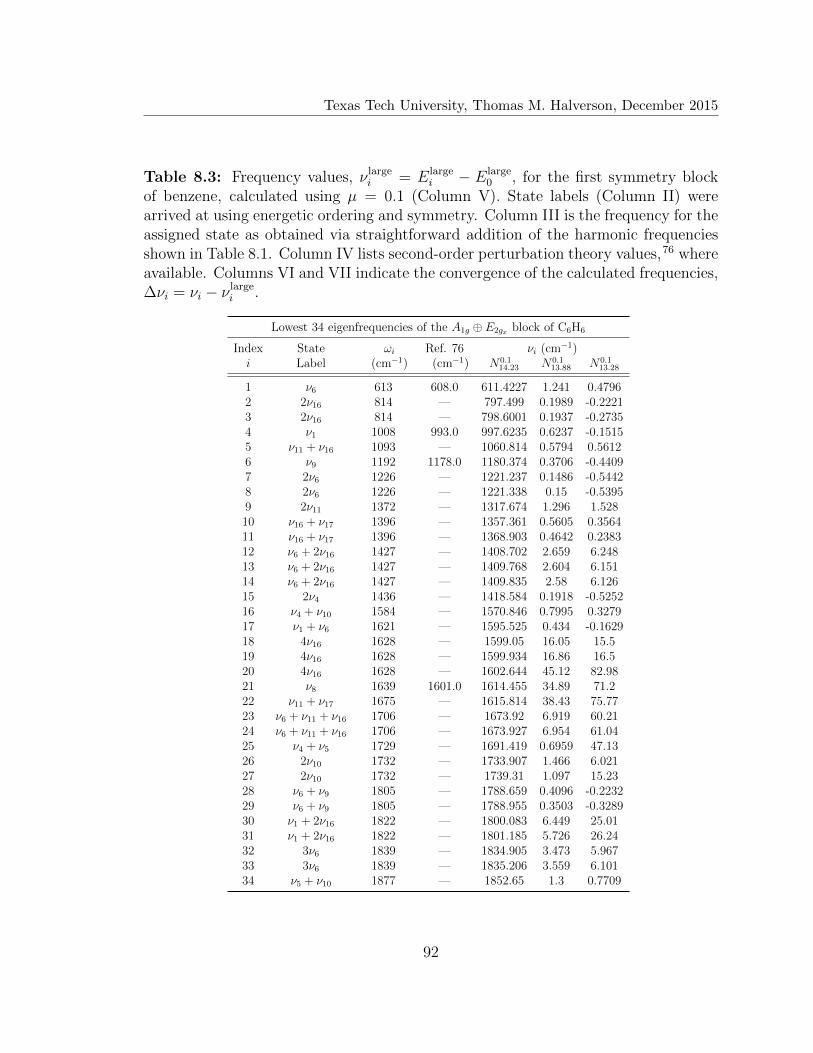
Texas Tech University, Thomas M. Halverson, December 2015
Table 8.3: Frequency values, ν largei = Elarge
i − Elarge0 , for the first symmetry block
of benzene, calculated using µ = 0.1 (Column V). State labels (Column II) werearrived at using energetic ordering and symmetry. Column III is the frequency for theassigned state as obtained via straightforward addition of the harmonic frequenciesshown in Table 8.1. Column IV lists second-order perturbation theory values,76 whereavailable. Columns VI and VII indicate the convergence of the calculated frequencies,∆νi = νi − ν large
i .
Lowest 34 eigenfrequencies of the A1g ⊕ E2gx block of C6H6
Index State ωi Ref. 76 νi (cm−1)i Label (cm−1) (cm−1) N0.1
14.23 N0.113.88 N0.1
13.28
1 ν6 613 608.0 611.4227 1.241 0.47962 2ν16 814 — 797.499 0.1989 -0.22213 2ν16 814 — 798.6001 0.1937 -0.27354 ν1 1008 993.0 997.6235 0.6237 -0.15155 ν11 + ν16 1093 — 1060.814 0.5794 0.56126 ν9 1192 1178.0 1180.374 0.3706 -0.44097 2ν6 1226 — 1221.237 0.1486 -0.54428 2ν6 1226 — 1221.338 0.15 -0.53959 2ν11 1372 — 1317.674 1.296 1.52810 ν16 + ν17 1396 — 1357.361 0.5605 0.356411 ν16 + ν17 1396 — 1368.903 0.4642 0.238312 ν6 + 2ν16 1427 — 1408.702 2.659 6.24813 ν6 + 2ν16 1427 — 1409.768 2.604 6.15114 ν6 + 2ν16 1427 — 1409.835 2.58 6.12615 2ν4 1436 — 1418.584 0.1918 -0.525216 ν4 + ν10 1584 — 1570.846 0.7995 0.327917 ν1 + ν6 1621 — 1595.525 0.434 -0.162918 4ν16 1628 — 1599.05 16.05 15.519 4ν16 1628 — 1599.934 16.86 16.520 4ν16 1628 — 1602.644 45.12 82.9821 ν8 1639 1601.0 1614.455 34.89 71.222 ν11 + ν17 1675 — 1615.814 38.43 75.7723 ν6 + ν11 + ν16 1706 — 1673.92 6.919 60.2124 ν6 + ν11 + ν16 1706 — 1673.927 6.954 61.0425 ν4 + ν5 1729 — 1691.419 0.6959 47.1326 2ν10 1732 — 1733.907 1.466 6.02127 2ν10 1732 — 1739.31 1.097 15.2328 ν6 + ν9 1805 — 1788.659 0.4096 -0.223229 ν6 + ν9 1805 — 1788.955 0.3503 -0.328930 ν1 + 2ν16 1822 — 1800.083 6.449 25.0131 ν1 + 2ν16 1822 — 1801.185 5.726 26.2432 3ν6 1839 — 1834.905 3.473 5.96733 3ν6 1839 — 1835.206 3.559 6.10134 ν5 + ν10 1877 — 1852.65 1.3 0.7709
92

Texas Tech University, Thomas M. Halverson, December 2015
Table 8.4: Frequency values for the second symmetry block of benzene calculatedusing µ = 0.1 truncation (see Table 8.3 for further details).
Lowest 26 eigenfrequencies for the A2g ⊕ E2gy block of C6H6
Index State ωi Ref. 76 νi (cm−1)i Label (cm−1) (cm−1) N0.1
14.23 N0.113.88 N0.1
13.28
1 ν6 613 608.0 611.4227 1.241 0.47962 2ν16 814 — 798.6001 0.1937 -0.27353 ν11 + ν16 1093 — 1060.814 0.5794 0.56124 ν9 1192 1178.0 1180.374 0.3706 -0.44095 2ν6 1226 — 1221.237 0.1486 -0.54426 ν3 1390 1350.0 1352.563 0.3641 -0.18827 ν16 + ν17 1396 — 1357.361 0.5605 0.35648 ν16 + ν17 1396 — 1375.937 0.2826 -0.35059 ν6 + 2ν16 1427 — 1408.702 2.659 6.24810 ν6 + 2ν16 1427 — 1409.736 2.59 6.13911 ν6 + 2ν16 1427 — 1409.768 2.604 6.15112 ν4 + ν10 1584 — 1570.846 0.7995 0.327913 ν1 + ν6 1621 — 1595.525 0.434 -0.162914 4ν16 1628 — 1599.934 15.17 14.6115 4ν16 1628 — 1602.644 14.15 13.7916 ν8 1639 1601.0 1614.455 34.89 71.117 ν11 + ν17 1675 — 1615.814 38.43 69.8418 ν6 + ν11 + ν16 1706 — 1673.811 6.997 64.7419 ν6 + ν11 + ν16 1706 — 1673.927 6.954 66.20 2ν10 1732 — 1739.31 1.097 15.2321 ν6 + ν9 1805 — 1787.628 0.3808 -0.264522 ν6 + ν9 1805 — 1788.955 0.3503 -0.328923 ν1 + 2ν16 1822 — 1801.185 5.726 23.9124 3ν6 1839 — 1834.89 3.475 5.96825 3ν6 1839 — 1835.206 3.559 6.10126 ν5 + ν10 1877 — 1852.65 1.3 0.7709
93
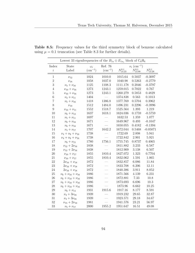
Texas Tech University, Thomas M. Halverson, December 2015
Table 8.5: Frequency values for the third symmetry block of benzene calculatedusing µ = 0.1 truncation (see Table 8.3 for further details).
Lowest 33 eigenfrequencies of the B1u ⊕ E1ux block of C6H6
Index State ωi Ref. 76 νi (cm−1)i Label (cm−1) (cm−1) N0.1
14.23 N0.113.88 N0.1
13.28
1 ν12 1024 1010.0 1015.64 0.5037 -0.30972 ν18 1058 1037.0 1040.98 0.5263 -0.27793 ν4 + ν16 1125 1108.3 1111.178 0.2046 -0.37974 ν10 + ν16 1273 1243.1 1259.015 0.7022 0.7675 ν10 + ν16 1273 1243.1 1260.279 0.5853 0.48296 ν4 + ν11 1404 — 1374.838 0.563 0.10137 ν5 + ν16 1418 1386.8 1377.769 0.5704 0.39628 ν19 1512 1484.0 1496.231 0.2296 -0.39969 ν10 + ν11 1552 1518.7 1525.564 1.393 1.21910 ν6 + ν12 1637 1618.1 1624.036 0.1759 -0.575911 ν5 + ν11 1697 — 1632.53 1.359 1.07712 ν6 + ν18 1671 — 1649.967 0.493 -0.104713 ν6 + ν18 1671 — 1650.055 0.4182 -0.139414 ν4 + ν17 1707 1642.2 1672.044 0.5468 -0.0507115 ν4 + ν6 + ν16 1738 — 1722.69 2.898 5.94116 ν4 + ν6 + ν16 1738 — 1722.842 2.901 5.92117 ν6 + ν15 1780 1756.1 1755.745 0.8737 0.406518 ν12 + 2ν16 1838 — 1811.882 3.233 6.58719 ν12 + 2ν16 1838 — 1812.909 3.138 6.50720 ν10 + ν17 1855 1810.4 1827.072 1.323 0.770421 ν10 + ν17 1855 1810.4 1832.062 1.591 1.06522 2ν16 + ν18 1872 — 1832.857 6.086 11.8423 2ν16 + ν18 1872 — 1833.708 6.206 12.1124 2ν16 + ν18 1872 — 1840.386 3.911 8.05225 ν6 + ν10 + ν16 1886 — 1871.566 4.139 6.23126 ν6 + ν10 + ν16 1886 — 1872.881 7.33 10.827 ν6 + ν10 + ν16 1886 — 1873.693 6.696 10.328 ν6 + ν10 + ν16 1886 — 1873.96 6.662 10.2529 ν6 + ν14 1931 1915.6 1917.16 8.177 8.59130 ν4 + 3ν16 1939 — 1919.232 29.65 32.8731 ν4 + 3ν16 1939 — 1923.571 29.18 34.6732 ν15 + 2ν16 1981 — 1941.576 23.21 56.9733 ν5 + ν17 2000 1955.2 1951.647 16.51 49.08
94

Texas Tech University, Thomas M. Halverson, December 2015
Table 8.6: Frequency values for the fourth symmetry block of benzene calculatedusing µ = 0.1 truncation (see Table 8.3 for further details).
Lowest 34 eigenfrequencies of the B2u ⊕ E1uy block of C6H6
Index State ωi Ref. 76 νi (cm−1)i Label (cm−1) (cm−1) N0.1
14.23 N0.113.88 N0.1
13.28
1 ν18 1058 1037.0 1040.98 0.5263 -0.27792 ν4 + ν16 1125 1108.3 1111.178 0.2046 -0.37973 ν15 1167 1150.0 1147.751 0.4723 -0.32264 ν10 + ν16 1273 1243.1 1260.279 0.5853 0.47355 ν10 + ν16 1273 1243.1 1260.781 0.407 -0.018926 ν14 1318 1309.0 1315.612 0.2943 -0.42297 ν5 + ν16 1418 1386.8 1377.769 0.5704 0.39628 ν19 1512 1484.0 1496.231 0.2296 -0.39969 ν10 + ν11 1552 1518.7 1525.564 1.393 1.21910 ν6 + ν12 1637 1618.1 1624.036 0.1759 -0.575911 ν6 + ν18 1671 — 1649.085 0.4198 -0.177612 ν6 + ν18 1671 — 1650.055 0.4058 -0.191913 ν4 + ν17 1707 1642.2 1672.044 0.5468 -0.0507114 ν4 + ν6 + ν16 1738 — 1722.842 2.901 5.92115 ν4 + ν6 + ν16 1738 — 1722.936 2.913 5.92116 ν6 + ν15 1780 1756.1 1755.745 0.8737 0.406517 ν12 + 2ν16 1838 — 1812.909 3.138 6.50718 ν10 + ν17 1855 1810.4 1827.072 1.323 0.770419 ν10 + ν17 1855 1810.4 1832.857 1.429 0.840620 2ν16 + ν18 1872 — 1833.006 5.937 11.6921 2ν16 + ν18 1872 — 1833.858 5.811 11.722 2ν16 + ν18 1872 — 1840.386 3.911 8.05223 ν6 + ν10 + ν16 1886 — 1871.566 4.139 6.23124 ν6 + ν10 + ν16 1886 — 1872.881 7.117 10.7325 ν6 + ν10 + ν16 1886 — 1873.205 7.006 10.4826 ν6 + ν10 + ν16 1886 — 1873.693 6.696 10.327 ν6 + ν14 1931 1915.6 1917.16 8.177 8.59128 ν4 + 3ν16 1939 — 1919.498 28.69 32.6129 ν4 + 3ν16 1939 — 1923.571 25.31 33.7730 ν15 + 2ν16 1981 — 1940.87 11.88 17.3731 ν15 + 2ν16 1981 — 1941.576 23.21 56.9732 ν5 + ν17 2000 1955.2 1951.647 16.86 49.2833 ν4 + ν6 + ν11 2017 — 1988.645 7.355 12.4634 ν5 + ν6 + ν16 2031 — 1991.223 6.859 43.71
95
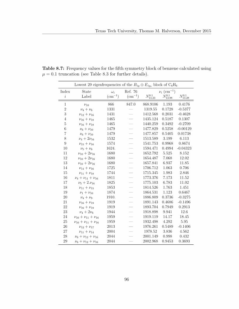
Texas Tech University, Thomas M. Halverson, December 2015
Table 8.7: Frequency values for the fifth symmetry block of benzene calculated usingµ = 0.1 truncation (see Table 8.3 for further details).
Lowest 29 eigenfrequencies of the B1g ⊕ E1gx block of C6H6
Index State ωi Ref. 76 νi (cm−1)i Label (cm−1) (cm−1) N0.1
14.23 N0.113.88 N0.1
13.28
1 ν10 866 847.0 868.9106 1.193 0.41762 ν4 + ν6 1331 — 1319.55 0.1728 -0.53773 ν12 + ν16 1431 — 1412.568 0.2031 -0.46284 ν16 + ν18 1465 — 1435.124 0.5187 0.13075 ν16 + ν18 1465 — 1440.259 0.3492 -0.27096 ν6 + ν10 1479 — 1477.829 0.5258 -0.001297 ν6 + ν10 1479 — 1477.857 0.5405 0.017388 ν4 + 2ν16 1532 — 1513.589 3.199 6.1139 ν15 + ν16 1574 — 1541.753 0.9968 0.867410 ν5 + ν6 1624. — 1594.471 0.4994 -0.0432311 ν10 + 2ν16 1680 — 1652.792 5.525 8.15212 ν10 + 2ν16 1680 — 1654.487 7.068 12.0213 ν10 + 2ν16 1680 — 1657.841 6.937 11.8514 ν14 + ν16 1725 — 1706.712 1.063 0.70615 ν11 + ν18 1744 — 1715.345 1.983 2.84616 ν4 + ν11 + ν16 1811 — 1773.376 7.173 11.5217 ν5 + 2.ν16 1825 — 1775.103 6.783 11.0218 ν11 + ν15 1853 — 1814.526 1.763 1.45119 ν1 + ν10 1874 — 1864.531 1.123 0.646720 ν4 + ν9 1910. — 1886.809 0.3736 -0.327521 ν16 + ν19 1919 — 1891.143 0.4686 -0.149622 ν16 + ν19 1919 — 1893.704 0.7949 0.291323 ν4 + 2ν6 1944 — 1918.898 9.941 12.624 ν10 + ν11 + ν16 1959 — 1919.119 14.17 18.4525 ν10 + ν11 + ν16 1959 — 1932.498 4.292 5.9526 ν12 + ν17 2013 — 1976.261 0.5489 -0.140627 ν11 + ν14 2004 — 1978.52 3.836 4.56228 ν6 + ν12 + ν16 2044 — 2001.149 0.998 0.43229 ν6 + ν12 + ν16 2044 — 2002.968 0.9453 0.3693
96
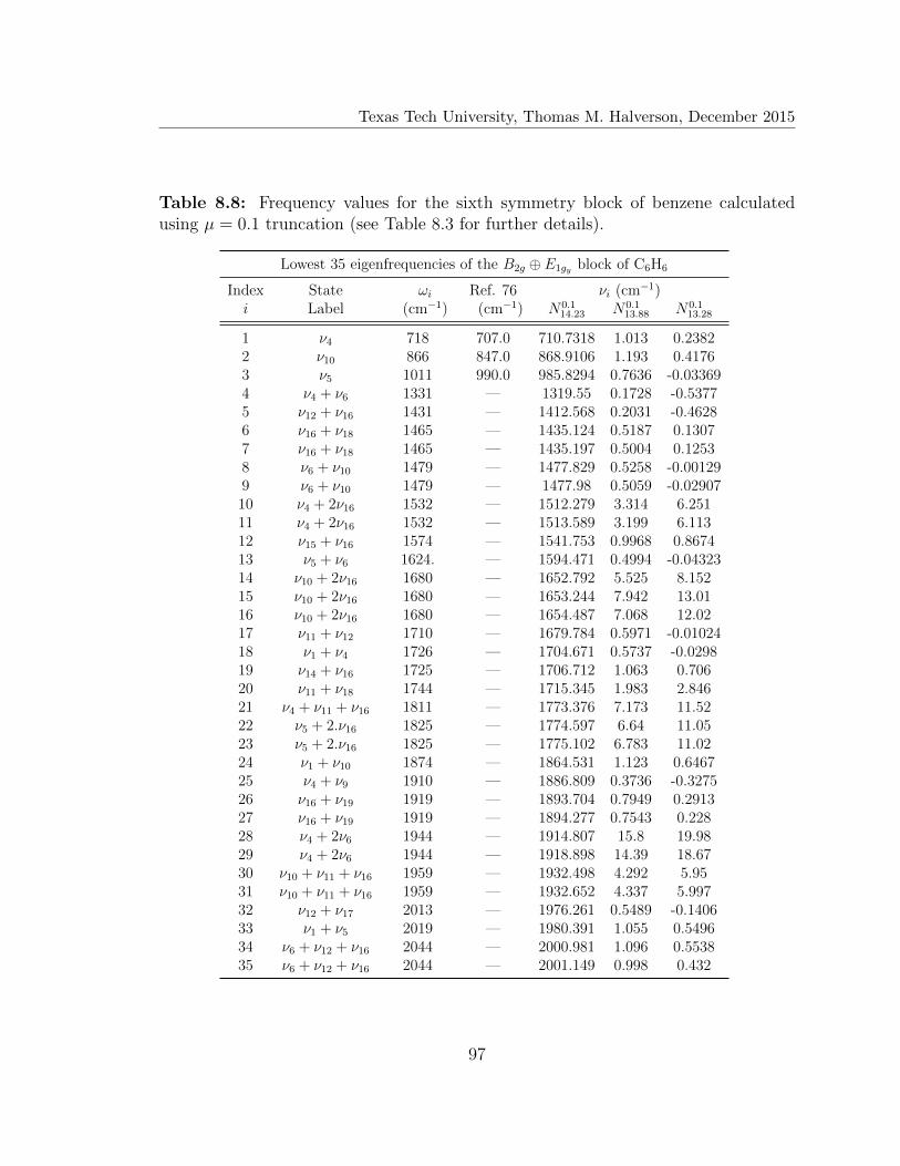
Texas Tech University, Thomas M. Halverson, December 2015
Table 8.8: Frequency values for the sixth symmetry block of benzene calculatedusing µ = 0.1 truncation (see Table 8.3 for further details).
Lowest 35 eigenfrequencies of the B2g ⊕ E1gy block of C6H6
Index State ωi Ref. 76 νi (cm−1)i Label (cm−1) (cm−1) N0.1
14.23 N0.113.88 N0.1
13.28
1 ν4 718 707.0 710.7318 1.013 0.23822 ν10 866 847.0 868.9106 1.193 0.41763 ν5 1011 990.0 985.8294 0.7636 -0.033694 ν4 + ν6 1331 — 1319.55 0.1728 -0.53775 ν12 + ν16 1431 — 1412.568 0.2031 -0.46286 ν16 + ν18 1465 — 1435.124 0.5187 0.13077 ν16 + ν18 1465 — 1435.197 0.5004 0.12538 ν6 + ν10 1479 — 1477.829 0.5258 -0.001299 ν6 + ν10 1479 — 1477.98 0.5059 -0.0290710 ν4 + 2ν16 1532 — 1512.279 3.314 6.25111 ν4 + 2ν16 1532 — 1513.589 3.199 6.11312 ν15 + ν16 1574 — 1541.753 0.9968 0.867413 ν5 + ν6 1624. — 1594.471 0.4994 -0.0432314 ν10 + 2ν16 1680 — 1652.792 5.525 8.15215 ν10 + 2ν16 1680 — 1653.244 7.942 13.0116 ν10 + 2ν16 1680 — 1654.487 7.068 12.0217 ν11 + ν12 1710 — 1679.784 0.5971 -0.0102418 ν1 + ν4 1726 — 1704.671 0.5737 -0.029819 ν14 + ν16 1725 — 1706.712 1.063 0.70620 ν11 + ν18 1744 — 1715.345 1.983 2.84621 ν4 + ν11 + ν16 1811 — 1773.376 7.173 11.5222 ν5 + 2.ν16 1825 — 1774.597 6.64 11.0523 ν5 + 2.ν16 1825 — 1775.102 6.783 11.0224 ν1 + ν10 1874 — 1864.531 1.123 0.646725 ν4 + ν9 1910 — 1886.809 0.3736 -0.327526 ν16 + ν19 1919 — 1893.704 0.7949 0.291327 ν16 + ν19 1919 — 1894.277 0.7543 0.22828 ν4 + 2ν6 1944 — 1914.807 15.8 19.9829 ν4 + 2ν6 1944 — 1918.898 14.39 18.6730 ν10 + ν11 + ν16 1959 — 1932.498 4.292 5.9531 ν10 + ν11 + ν16 1959 — 1932.652 4.337 5.99732 ν12 + ν17 2013 — 1976.261 0.5489 -0.140633 ν1 + ν5 2019 — 1980.391 1.055 0.549634 ν6 + ν12 + ν16 2044 — 2000.981 1.096 0.553835 ν6 + ν12 + ν16 2044 — 2001.149 0.998 0.432
97
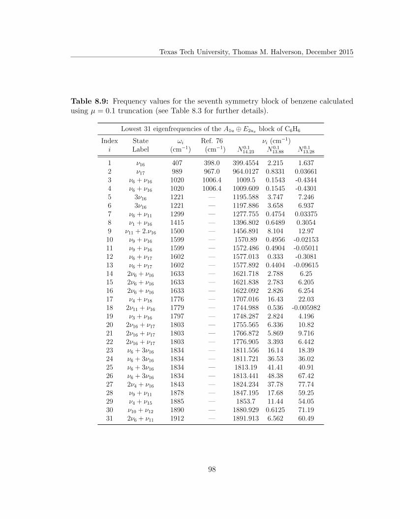
Texas Tech University, Thomas M. Halverson, December 2015
Table 8.9: Frequency values for the seventh symmetry block of benzene calculatedusing µ = 0.1 truncation (see Table 8.3 for further details).
Lowest 31 eigenfrequencies of the A1u ⊕ E2ux block of C6H6
Index State ωi Ref. 76 νi (cm−1)i Label (cm−1) (cm−1) N0.1
14.23 N0.113.88 N0.1
13.28
1 ν16 407 398.0 399.4554 2.215 1.6372 ν17 989 967.0 964.0127 0.8331 0.036613 ν6 + ν16 1020 1006.4 1009.5 0.1543 -0.43444 ν6 + ν16 1020 1006.4 1009.609 0.1545 -0.43015 3ν16 1221 — 1195.588 3.747 7.2466 3ν16 1221 — 1197.886 3.658 6.9377 ν6 + ν11 1299 — 1277.755 0.4754 0.033758 ν1 + ν16 1415 — 1396.802 0.6489 0.30549 ν11 + 2.ν16 1500 — 1456.891 8.104 12.9710 ν9 + ν16 1599 — 1570.89 0.4956 -0.0215311 ν9 + ν16 1599 — 1572.486 0.4904 -0.0501112 ν6 + ν17 1602 — 1577.013 0.333 -0.308113 ν6 + ν17 1602 — 1577.892 0.4404 -0.0961514 2ν6 + ν16 1633 — 1621.718 2.788 6.2515 2ν6 + ν16 1633 — 1621.838 2.783 6.20516 2ν6 + ν16 1633 — 1622.092 2.826 6.25417 ν4 + ν18 1776 — 1707.016 16.43 22.0318 2ν11 + ν16 1779 — 1744.988 0.536 -0.00598219 ν3 + ν16 1797 — 1748.287 2.824 4.19620 2ν16 + ν17 1803 — 1755.565 6.336 10.8221 2ν16 + ν17 1803 — 1766.872 5.869 9.71622 2ν16 + ν17 1803 — 1776.905 3.393 6.44223 ν6 + 3ν16 1834 — 1811.556 16.14 18.3924 ν6 + 3ν16 1834 — 1811.721 36.53 36.0225 ν6 + 3ν16 1834 — 1813.19 41.41 40.9126 ν6 + 3ν16 1834 — 1813.441 48.38 67.4227 2ν4 + ν16 1843 — 1824.234 37.78 77.7428 ν9 + ν11 1878 — 1847.195 17.68 59.2529 ν4 + ν15 1885 — 1853.7 11.44 54.0530 ν10 + ν12 1890 — 1880.929 0.6125 71.1931 2ν6 + ν11 1912 — 1891.913 6.562 60.49
98
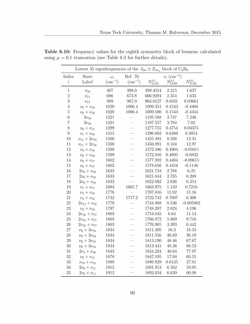
Texas Tech University, Thomas M. Halverson, December 2015
Table 8.10: Frequency values for the eighth symmetry block of benzene calculatedusing µ = 0.1 truncation (see Table 8.3 for further details).
Lowest 35 eigenfrequencies of the A2u ⊕ E2uy block of C6H6
Index State ωi Ref. 76 νi (cm−1)i Label (cm−1) (cm−1) N0.1
14.23 N0.113.88 N0.1
13.28
1 ν16 407 398.0 399.4554 2.215 1.6372 ν11 686 673.8 666.9294 2.354 1.6333 ν17 989 967.0 964.0127 0.8331 0.036614 ν6 + ν16 1020 1006.4 1009.351 0.1543 -0.43685 ν6 + ν16 1020 1006.4 1009.500 0.1543 -0.43446 3ν16 1221 — 1195.588 3.747 7.2467 3ν16 1221 — 1197.557 3.704 7.028 ν6 + ν11 1299 — 1277.755 0.4754 0.033759 ν1 + ν16 1415 — 1396.802 0.6489 0.305410 ν11 + 2ν16 1500 — 1455.491 8.338 13.3111 ν11 + 2ν16 1500 — 1456.891 8.104 12.9712 ν9 + ν16 1599 — 1572.486 0.4904 -0.0501113 ν9 + ν16 1599 — 1572.916 0.4695 -0.083214 ν6 + ν17 1602 — 1577.892 0.4404 -0.0961515 ν6 + ν17 1602 — 1578.656 0.4416 -0.114616 2ν6 + ν16 1633 — 1621.718 2.788 6.2517 2ν6 + ν16 1633 — 1621.844 2.785 6.20818 2ν6 + ν16 1633 — 1622.092 2.826 6.25419 ν1 + ν11 1694 1665.7 1663.975 1.133 0.721620 ν4 + ν18 1776 — 1707.016 15.92 15.1621 ν4 + ν12 1742 1717.2 1722.742 0.7007 6.30622 2ν11 + ν16 1779 — 1744.988 0.536 -0.00598223 ν3 + ν16 1797 — 1748.287 2.824 4.19624 2ν16 + ν17 1803 — 1754.645 6.64 11.1425 2ν16 + ν17 1803 — 1766.872 5.869 9.71626 2ν16 + ν17 1803 — 1776.905 3.393 6.44227 ν6 + 3ν16 1834 — 1811.395 16.3 18.5528 ν6 + 3ν16 1834 — 1811.556 36.69 36.1929 ν6 + 3ν16 1834 — 1813.190 48.46 67.6730 ν6 + 3ν16 1834 — 1813.441 48.38 88.5331 2ν4 + ν16 1843 — 1824.234 40.64 77.9732 ν9 + ν11 1878 — 1847.195 17.94 60.5533 ν10 + ν12 1890 — 1880.929 0.6125 27.0134 2ν6 + ν11 1912 — 1891.913 6.562 59.9535 2ν6 + ν11 1912 — 1892.034 6.639 60.08
99
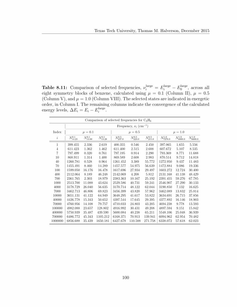
Texas Tech University, Thomas M. Halverson, December 2015
Table 8.11: Comparison of selected frequencies, ν largei = Elarge
i − Elarge0 , across all
eight symmetry blocks of benzene, calculated using µ = 0.1 (Column II), µ = 0.5(Column V), and µ = 1.0 (Column VIII). The selected states are indicated in energeticorder, in Column I. The remaining columns indicate the convergence of the calculatedenergy levels, ∆Ei = Ei − Elarge
i .
Comparison of selected frequencies for C6H6
Frequency, νi (cm−1)
Index µ = 0.1 µ = 0.5 µ = 1.0
i N0.114.23 N0.1
13.88 N0.113.28 N0.5
237.0 N0.5223.0 N0.5
215.0 N1.07278.0 N1.0
6800.0 N1.06600.0
1 399.455 2.336 2.619 400.355 0.546 2.450 397.065 1.655 5.5564 611.423 1.362 1.462 611.400 2.515 2.688 607.672 5.107 8.5357 797.499 0.320 0.761 797.195 0.914 2.290 793.369 8.771 11.68810 868.911 1.314 1.400 869.589 2.608 2.983 870.514 9.712 14.81840 1260.781 0.528 0.964 1261.452 3.389 55.772 1272.950 9.437 11.48370 1455.491 8.460 14.289 1457.577 54.975 56.639 1472.884 9.086 19.336100 1599.050 16.176 16.478 1617.696 27.934 29.497 1603.272 12.724 30.400400 2112.064 8.189 46.248 2142.069 4.208 5.812 2131.168 41.138 48.429700 2361.765 2.303 18.979 2383.363 10.167 25.192 2391.455 59.276 67.7851000 2513.700 11.088 43.624 2529.586 40.731 59.241 2546.907 27.290 30.1334000 3178.729 26.040 56.635 3170.714 48.122 62.044 3190.850 7.132 16.6257000 3462.713 46.806 69.823 3456.399 43.820 57.962 3462.089 13.832 25.81410000 3651.131 41.122 64.949 3648.295 41.617 53.822 3634.691 26.715 37.85640000 4426.778 15.343 50.652 4397.544 17.645 29.395 4377.892 16.146 18.90370000 4760.956 14.108 79.757 4710.033 24.803 43.205 4694.238 9.778 13.593100000 4982.088 23.657 128.802 4916.992 30.431 49.208 4897.594 9.151 15.842400000 5750.939 35.487 439.590 5600.084 40.238 65.211 5548.106 25.048 36.939700000 6486.772 45.343 1105.212 6168.371 70.913 139.941 6094.962 62.954 70.4821000000 6856.688 35.439 1650.181 6427.678 110.588 271.758 6338.072 57.618 62.023
100
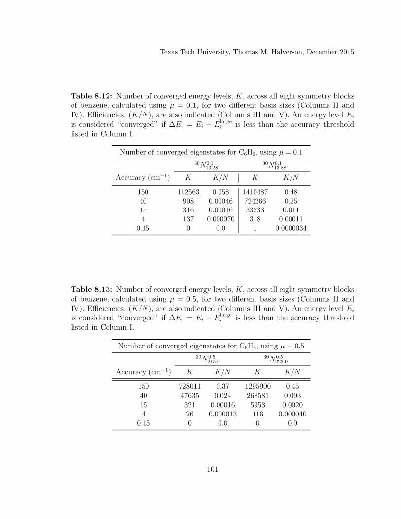
Texas Tech University, Thomas M. Halverson, December 2015
Table 8.12: Number of converged energy levels, K, across all eight symmetry blocksof benzene, calculated using µ = 0.1, for two different basis sizes (Columns II andIV). Efficiencies, (K/N), are also indicated (Columns III and V). An energy level Eiis considered “converged” if ∆Ei = Ei − Elarge
i is less than the accuracy thresholdlisted in Column I.
Number of converged eigenstates for C6H6, using µ = 0.1
30N0.113.28
30N0.113.88
Accuracy (cm−1) K K/N K K/N
150 112563 0.058 1410487 0.4840 908 0.00046 724266 0.2515 316 0.00016 33233 0.0114 137 0.000070 318 0.00011
0.15 0 0.0 1 0.0000034
Table 8.13: Number of converged energy levels, K, across all eight symmetry blocksof benzene, calculated using µ = 0.5, for two different basis sizes (Columns II andIV). Efficiencies, (K/N), are also indicated (Columns III and V). An energy level Eiis considered “converged” if ∆Ei = Ei − Elarge
i is less than the accuracy thresholdlisted in Column I.
Number of converged eigenstates for C6H6, using µ = 0.5
30N0.5215.0
30N0.5223.0
Accuracy (cm−1) K K/N K K/N
150 728011 0.37 1295900 0.4540 47635 0.024 268581 0.09315 321 0.00016 5953 0.00204 26 0.000013 116 0.000040
0.15 0 0.0 0 0.0
101

Texas Tech University, Thomas M. Halverson, December 2015
Table 8.14: Number of converged energy levels, K, across all eight symmetry blocksof benzene, calculated using µ = 1.0, for two different basis sizes (Columns II andIV). Efficiencies, (K/N), are also indicated (Columns III and V). An energy level Eiis considered “converged” if ∆Ei = Ei − Elarge
i is less than the accuracy thresholdlisted in Column I.
Number of converged eigenstates for C6H6, using µ = 0.5
30N1.06600.0
30N1.06800.0
Accuracy (cm−1) K K/N K K/N
150 1983268 0.96 2688080 0.9640 974760 0.47 1843956 0.6615 48410 0.023 652066 0.234 1 0.0000048 3 0.000011
0.15 0 0.0 0 0.0
Table 8.15: Total number of energy levels, Nµ, contributed to the HT dataset fromµ = 0.1 (Column IV), µ = 0.5 (Column V), and µ = 1.0 (Column VI), for each of theeight symmetry blocks of benzene. The total HT dataset size, NHT is indicated inColumn III for each block. Totals across all eight symmetry blocks are listed in thelast row.
Number of states chosen during the hybrid process
Symmetry NHT Nµ
Block D6h irreps µ = 0.1 µ = 0.5 µ = 1.0
1 A1g ⊕ E2gx 716205 1566 49511 6651282 A2g ⊕ E2gy 713919 1498 49053 6633683 B1u ⊕ E1ux 712008 2244 48405 6613594 B2u ⊕ E1uy 711428 2204 47852 6613725 B1g ⊕ E1gx 707327 2171 43976 6611806 B2g ⊕ E1gy 709084 2215 43993 6628767 A1u ⊕ E2ux 708032 1613 48174 6582458 A2u ⊕ E2uy 709057 1548 48357 659152
total 5687060 15059 379321 5292680
102
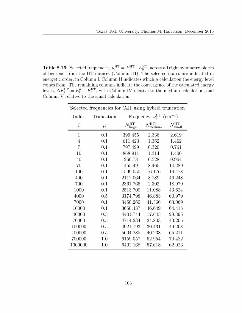
Texas Tech University, Thomas M. Halverson, December 2015
Table 8.16: Selected frequencies, νHTi = EHT
i −EHT0 , across all eight symmetry blocks
of benzene, from the HT dataset (Column III). The selected states are indicated inenergetic order, in Column I. Column II indicates which µ calculation the energy levelcomes from. The remaining columns indicate the convergence of the calculated energylevels, ∆EHT
i = Eµi − EHT
i , with Column IV relative to the medium calculation, andColumn V relative to the small calculation.
Selected frequencies for C6H6using hybrid truncation
Index Truncation Frequency, νHTi (cm−1)
i µ NHTlarge NHT
medium NHTsmall
1 0.1 399.455 2.336 2.6194 0.1 611.423 1.362 1.4627 0.1 797.499 0.320 0.76110 0.1 868.911 1.314 1.40040 0.1 1260.781 0.528 0.96470 0.1 1455.491 8.460 14.289100 0.1 1599.050 16.176 16.478400 0.1 2112.064 8.189 46.248700 0.1 2361.765 2.303 18.9791000 0.1 2513.700 11.088 43.6244000 0.5 3174.798 46.883 60.9797000 0.1 3460.260 41.366 63.06910000 0.1 3650.437 46.649 64.41540000 0.5 4401.744 17.645 29.39570000 0.5 4714.234 24.803 43.205100000 0.5 4921.193 30.431 49.208400000 0.5 5604.285 40.238 65.211700000 1.0 6159.057 62.954 70.4821000000 1.0 6402.168 57.618 62.023
103
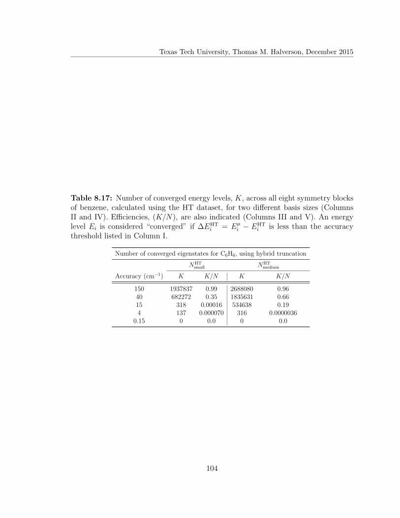
Texas Tech University, Thomas M. Halverson, December 2015
Table 8.17: Number of converged energy levels, K, across all eight symmetry blocksof benzene, calculated using the HT dataset, for two different basis sizes (ColumnsII and IV). Efficiencies, (K/N), are also indicated (Columns III and V). An energylevel Ei is considered “converged” if ∆EHT
i = Eµi − EHT
i is less than the accuracythreshold listed in Column I.
Number of converged eigenstates for C6H6, using hybrid truncation
NHTsmall NHT
medium
Accuracy (cm−1) K K/N K K/N
150 1937837 0.99 2688080 0.9640 682272 0.35 1835631 0.6615 318 0.00016 534638 0.194 137 0.000070 316 0.0000036
0.15 0 0.0 0 0.0
104
Texas Tech University, Thomas M. Halverson, December 2015
CHAPTER 9
CLOSING REMARKS
There appears to an apparent ebb and flow in computational technology. In
the late 90’s we saw a revolution in the decrease in size of computing power. Plat-
forms that would fill entire rooms only a few years earlier, were packed into compact
personal systems. Recently, we have seen the rebirth of very large computational
systems, that again fill entire rooms. Most likely in the coming years we will see
this technology “shrink” again, but before that becomes the case, these new immense
systems have at the very least allowed for new benchmarks to be set. It is pivotal
that computational software be developed to take advantage of the current technol-
ogy. Enter SwitchBLADE, a software package that does exactly that. The speed
at which technology changes, may soon render codes like SwitchBLADE obsolete
in the future, but that does not mean that much cannot be learned in the meantime.
In its early implementation, SwitchBLADE showcased the power of a basis set
that formally defeats exponential scaling. In Chapters 4, 5, and 6 we showed that
PSLB’s which are collectively well localized can be used to dramatically increase basis
efficiency. The essential additions that make the methods discussed here different
from previous studies are momentum symmetrization and phase space truncation.
The former allows the latter, since without the former, the latter is impossible due
to the ideas discussed in Section 2.3. With those two properties in place, the SGB’s
provide a simple, universal basis set, which can be used to solve a myriad of problems.
Here, we explored model systems (IUHO) up to D = 27 with only a modest amount of
computational resources. Even in the more complicated case of systems with coupling
(CAHO), we were able to span from D = 3 to D = 16 using the same code. Beyond
simple models, the study of P2O and CH2NH proved that addition of negative energy
contributions to the Hamiltonian—i.e., odd powers of the position coordinates and/or
negative value coefficients in the FFP—did not hinder the performance of the SGB,
as long as the PST was completed in a smart way as to avoid exponential scaling (See
Sections 3.2 and 3.3). Using our simple, dimensionally independent code, we were
able to compute vibrational spectra for systems up to D = 9 in a reasonable amount
of time (< 24 hrs.) and utilizing a reasonable amount of computational resources
105
Texas Tech University, Thomas M. Halverson, December 2015
(< 5000 cores). Note, yet again, that both systems, P2O and CH2NH, were analyzed
using the same code, with zero modification. All that SwitchBLADE requires to
compute vibrational spectra is an FFP. This is a large and important step toward
the aforementioned goal of a do-it-all, black-box system.
All the effort that had gone into the study of phase space in the context of
how to properly create a collectively localized basis provided the machinery needed
to apply phase space ideas to other basis sets, namely HOB. The PSP described in
Section 2.2 turns out to be indispensable, and should prove to be quite useful in
other areas of study. Most likely, we have only begun to scratch the surface of what
this tool can provide. As for the applications utilized here, we were able to provide
the first (to our knowledge) theoretical study as to how energy truncation affects
the efficiency of HOB (See Section 2.4). Also, we have shown with our higher D
studies, CH3CN and C6H6, a single basis alone is not adequate to compute the entire
spectrum. The standard truncation method, µ = 0.0, has been utilized for some time
to compute the lower energy regime, but to go beyond this we need to utilize multiple
truncation types—i.e., hybrid truncation. Since SwitchBLADE provides a simple
way to compute multiple spectra, using a wide variety of truncation and different
basis sets, it provides the prefect tool to achieve this end.
In time, many additions could be made to improve the functionality of Switch-
BLADE (some of which were discussed in previous sections, e.g., PSRO’s). One such
addition not yet discussed is the calculations of the calculation of rotational (and pos-
sible rovibrational and rovibronic) energy states. To do this, we must first move past
FFP’s and utilize full PES’s. However, the advantage of using FFP’s is that we can
compute analytic matrix elements, and, therefore, the calculations are strictly varia-
tional. This is paramount if we wish to utilize hybridization, since our criterion is that
the lowest eigenenergy is most correct. However, if we move toward a more general
PES system, we will most likely have to utilize some sort of quadrature,77 eliminat-
ing the variational nature of the calculations. In any event, the implementation of
rotational motion would be straightforward if the rotational operators are expressed
in a Cartesian-like manner, as in the case of the Watson Hamiltonian,78 but if the
ultimate goal is to maximize accuracy and to truly calculate experimentally relevant,
spectroscopic rovibrational (or even rovibronic) energy levels, a full PES is the only
106

Texas Tech University, Thomas M. Halverson, December 2015
option. Though already a powerful tool for FFP systems, if computationally inex-
pensive quadrature, PSRO’s, and even sparse iterative methods can be successfully
incorporated, SwitchBLADE would become an even more formidable weapon than
it already is.
107
Texas Tech University, Thomas M. Halverson, December 2015
BIBLIOGRAPHY
[1] Bowman, J. M. Comp. Phys. Commun., Special Issue on “Molecular Vibrations”1988, 51, 225.
[2] Bowman, J. M. Acc. Chem. Res. 1986, 19, 202–208.
[3] Bacic, Z.; Light, J. C. Annu. Rev. Phys. Chem. 1989, 40, 469.
[4] Bramley, M. J.; Carrington, Jr., T. J. Chem. Phys. 1993, 99, 8519.
[5] Poirier, B.; Light, J. C. J. Chem. Phys. 1999, 111, 4869–4885.
[6] Poirier, B.; Light, J. C. J. Chem. Phys. 2000, 113, 211–217.
[7] Cullum, J. K.; Willoughby, R. A. Lanczos Algorithms for Large Symmetric Eigen-value Computations ; Birkhauser: Boston, 1985.
[8] Saad, Y. Iterative Methods for Sparse Linear Systems ; PWS: Boston, 1996.
[9] Light, J. C.; Carrington Jr., T. Adv. Chem. Phys. 2000, 114, 263.
[10] Avila, G.; Carrington, Jr., T. J. Chem. Phys. 2011, 134, 054126.
[11] Avila, G.; Carrington, Jr., T. J. Chem. Phys. 2012, 137, 184108.
[12] Petty, C.; Chen, W.; Poirier, B. J. Chem. Phys. A 2013, 137, 7280.
[13] Bracken, A. J.; Doebner, H.-D.; Wood, J. G. Phys. Rev. Lett. 1999, 83, 3758.
[14] Wood, J. G. Bounds on integrals of the Wigner function. Ph.D. thesis in physics,University of Queensland, St. Lucia 4072, Australia, 2003.
[15] Meyer, H.-D., Gatti, F., Worth, G. A., Eds. Multidimensional Quantum Dynam-ics: MCTDH Theory and Applications ; Wiley-VCH: Weinheim, 2009.
[16] Matyus, E.; Czako, G.; Csaszar, A. G. J. Chem. Phys. 2009, 130, 134112.
[17] Yurchenko, S. N.; Thiel, W.; Jensen, P. J. Mol. Spec. 2007, 245, 126–140.
[18] Davis, M. J.; Heller, E. J. J. Chem. Phys. 1979, 71, 3383.
[19] Poirier, B. J. Theo. Comput. Chem. 2003, 2, 65–72.
[20] Poirier, B.; Salam, A. J. Chem. Phys. 2004, 121, 1690–1703.
[21] Poirier, B.; Salam, A. J. Chem. Phys. 2004, 121, 1704–1724.
108

Texas Tech University, Thomas M. Halverson, December 2015
[22] Lombardini, R.; Poirier, B. Phys. Rev. E 2006, 74, 036705.
[23] Goedecker, S. Rev. Mod. Phys. 1999, 71, 1085–1123.
[24] Dennington, R.; Keith, T.; Millam, J. GaussView Version 5. Semichem Inc.Shawnee Mission KS 2009.
[25] Bacic, Z.; Light, J. C. J. Chem. Phys. 1986, 85, 4594.
[26] Cargo, M. C.; Littlejohn, R. G. Phys. Rev. E 2002, 65, 026703.
[27] Littlejohn, R. G.; Cargo, M.; Carrington, Jr., T.; Mitchell, K. A.; Poirier, B. J.Chem. Phys. 2002, 116, 8691.
[28] Fattal, E.; Baer, R.; Kosloff, R. Phys. Rev. E. 1996, 53, 1217.
[29] Poirier, B.; Light, J. C. J. Chem. Phys. 1999, 111, 4869–4885.
[30] Poirier, B.; Light, J. C. J. Chem. Phys. 2001, 114, 6562–6571.
[31] Bian, W.; Poirier, B. J. Theo. Comput. Chem. 2003, 2, 583–597.
[32] Weyl, H. Z. Phys. 1928, 46, 1.
[33] Wigner, E. Phys. Rev. 1932, 40, 749.
[34] Husimi, K. Proc. Phys. Math. Soc. Jpn. 1940, 22, 264.
[35] Moyal, J. E. Proc. Cambridge Phil. Soc. 1949, 45, 99.
[36] Hillery, M.; O’Connell, R. F.; Scully, M. O.; Wigner, E. P. Phys. Rep. 1984, 106,121–167.
[37] Lesche, B.; Seligman, T. H. J. Phys. A: Math. Gen. 1986, 19, 91–105.
[38] Poirier, B. Found. Phys. 2000, 30, 1191–1226.
[39] Shimshovitz, A.; Tannor, D. J. Phys. Rev. Lett. 2002, 109, 070402.
[40] Shimshovitz, A.; Tannor, D. J. arXiv.1207.0623v1 [math.FA].
[41] Mallet, S. G. IEEE Tans. Pattern Anal. Machine Intell. 1989, 11, 674–693.
[42] Mallet, S. G. A Wavelet Tour of Signal Processing ; Academic Press: Burlington,1998.
[43] von Neumann, J. Z. Phys. 1929, 57, 30.
109

Texas Tech University, Thomas M. Halverson, December 2015
[44] Lowdin, P.-O. Adv. Phys. 1956, 5, 1.
[45] Arias, T. A. Rev. Mod. Phys. 1999, 71, 267.
[46] Balian, R. C. R. Acad. Sc. Paris 1981, 292, 1357–1361.
[47] Low, F. A Passion for Physics—Essays in Honor of Geoffrey Chew ; World Sci-entific: Singapore, 1985; pp 17–22.
[48] Klauder, J. R.; Sudarshan, E. C. G. Fundamentals of Quantum Optics ; W. A.Benjamin, Inc.: New York, 1968.
[49] Perelemov, A. Generalized Coherent States and Their Applications ; Springer-Verlag: Berlin, 1986.
[50] Wilson, K. G. Generalized Wannier Functions. Cornell University preprint, 1987.
[51] Lombardini, R.; Poirier, B. J. Chem. Phys. 2006, 124, 144107.
[52] Carter, S.; Bowman, J. M.; Sharma, A. R. AIP Conf. Proc. 2012, 1504, 465–466.
[53] Wilson, Jr., E. B. Phys. Rev. 1934, 45, 706–714.
[54] Geus, R.; Rollin, S. Parallel Computing 2001, 27, 883–896.
[55] Gilbert, J. C.; Nocedal, J. SIAM J. Optimiz. 1992, 2, 21–42.
[56] Choi, J.; Dongarra, J.; Pozo, R.; Walker, D. in Proceedings of the Fourth Sympo-sium on the Frontiers of Massively Parallel Computation 1992, 120–127, IEEEComputer Society Press.
[57] http://www.research.ibm.com/bluegene.
[58] http://www.ncsa.uiuc.edu/BlueWaters/.
[59] Dawes, R.; Carrington, Jr., T. J. Chem. Phys. 2005, 122, 134101.
[60] Wang, Y.; Braams, B. J.; Bowman, J. M.; Carter, S.; Tew, D. P. J. Chem. Phys.2008, 128, 224314.
[61] Pouchan, C.; Aouni, M.; Begue, D. Chem. Phys. Lett. 2001, 334, 352–356.
[62] Bailleux, S.; Bogey, M.; Demuynck, C.; Destombes, J.; Lui, Y.; Csaszar, A. G.J. Chem. Phys. 1997, 107, 8317.
[63] Gulein, M.; Cernicharo, J.; Pauber, G.; Turner, B. E. Astron. Astrophys. 1990,230, L9–L11.
110
Texas Tech University, Thomas M. Halverson, December 2015
[64] Millar, T. J. Astron. Astrophys. 1991, 242, 241–246.
[65] Pahlevani, F.; Kitamura, S.; Shibata, H.; Maruoka, N. ISIJ Int. 2010, 50, 822–829.
[66] Ornellas, F.; Aquino, A. Theor. Chim. Acta. 1991, 79, 105–114.
[67] Johnson, B. R. Chem. Phys. Lett. 1972, 13, 172.
[68] Tang, Y.; Nielsen, C. J. Atmos. Environ. 2012, 55, 185–189.
[69] Pouchan, C.; Zaki, K. J. Chem. Phys. 1997, 107, 342.
[70] Begue, D.; Carbonniere, P.; Pouchan, C. J. Phys. Chem A 2005, 109, 4611–4616.
[71] Henry, L.; Amat, G. J. Mol. Spectrosc. 1960, 5, 319–325.
[72] Henry, L.; Amat, G. J. Mol. Spectrosc. 1965, 15, 168–179.
[73] Willetts, A.; Handy, N. C.; Green, W. H.; Jayatilaka, D. J. Phys. Chem. 1990,94, 5608.
[74] Gaw, J. F.; Willetts, A.; Green, W. H.; Handy, N. C. In Advances in MolecularVibrations and Collision Dynamics ; Bowmen, J. M., Ed.; JAI Press Inc.: NewYork, NY, 1991; Vol. IB; p 169.
[75] Goodman, L.; Ozkabak, A. G.; Thakur, S. N. J. Phys. Chem 1991, 95, 9044.
[76] Maslen, P. E.; Handy, N. C.; Amos, R. D.; Jayatilaka, D. J. Chem. Phys. 1992,97, 4233.
[77] Press et al, W. H. Numerical Recipes, 2nd ed.; Cambridge University Press:Cambridge, England, 1992.
[78] Watson, J. K. G. Mol. Phys. 1968, 15, 479–490.
111