ccopy 2020 Sarah Christensen

ALGORITHMS FOR PHYLOGENETIC TREE CORRECTION INSPECIES AND CANCER EVOLUTION

BY

SARAH CHRISTENSEN

DISSERTATION

Submitted in partial fulfillment of the requirementsfor the degree of Doctor of Philosophy in Computer Science

in the Graduate College of theUniversity of Illinois at Urbana-Champaign 2020

Urbana Illinois

Doctoral Committee

Assistant Professor Mohammed El-Kebir Chair and Director of ResearchProfessor Tandy Warnow Co-Director of ResearchProfessor Sariel Har-PeledProfessor Luay Nakhleh Rice University

ABSTRACT

Reconstructing evolutionary trees also known as phylogenies from molecular sequence

data is a fundamental problem in computational biology Classically evolutionary trees

have been estimated over a set of species where leaves correspond to extant species and

internal nodes correspond to ancestral species This type of phylogeny is colloquially thought

of as the ldquoTree of Liferdquo and assembling it has been designated as a Grand Challenge by

the National Science Foundation Advisory Committee for Cyberinfrastructure However

processes other than speciation are also shaped by evolution One notable example is in

the development of a malignant tumor tumor cells rapidly grow and divide acquiring new

mutations with each subsequent generation Tumor cells then compete for resources often

resulting in selection for more aggressive cell types Recent advancements in sequencing

technology rapidly increased the amount of sequencing data taken from tumor biopsies This

development has allowed researchers to attempt reconstructing evolutionary histories for

individual patient tumors improving our understanding of cancer and laying the groundwork

for precision therapy

Despite algorithmic improvements in the estimation of both species and tumor phylo-

genies from molecular sequence data current approaches still suffer a number of limita-

tions Incomplete sampling and estimation error can lead to missing leaves and low-support

branches in the estimated phylogenies Moreover commonly posed optimization problems

are often under-determined given the limited amounts and low quality of input data leading

to large solution spaces of equally plausible phylogenies In this dissertation we explore cur-

rent limitations in both species and tumor phylogeny estimation connecting similarities and

highlighting key differences We then put forward four new methods that improve phylogeny

estimation methods by incorporating auxiliary information OCTAL TRACTION PhySigs

and RECAP For each method we present theoretical results (eg optimization problem

complexity algorithmic correctness running time analysis) as well as empirical results on

simulated and real datasets Collectively these methods show we can significantly improve

the accuracy of leading phylogeny estimation methods by leveraging additional signal in

distinct but related datasets

ii

ACKNOWLEDGEMENTS

I would like to begin by thanking my advisors without whom this dissertation would not

be possible In particular I would like to thank Professor Tandy Warnow for taking a chance

on me when I first started my PhD with no background in computer science I am especially

grateful for her candor when giving advice her patience as I navigated my way through

graduate school and her support as I went on to explore new topics She is truly a role

model to young women scientists and I benefited immensely from her mentorship I would

also like to thank Professor Mohammed El-Kebir whose cheerful demeanor and optimism

helped me to keep pushing through the ups and downs of graduate school It is through

Mohammed that I was introduced to cancer genomics which connected the two types of

evolution that ultimately became my dissertation Most of all I appreciate Mohammed for

always encouraging me follow my own interests even when it led to him sitting through long

talks on complexity lower bounds

I also want to acknowledge other important people that helped my academic progres-

sion Specifically I would like to thank my Doctoral Committee including Professor Sariel

Har-Peled and Professor Luay Nakhleh for their thoughtful feedback and guidance Pro-

fessor Chandra Chekuri was also extremely generous with his time throughout my PhD

experience often offering a helpful outside perspective Moreover I would be remiss if I

did not thank all of my coauthors Juho Kim Erin K Molloy Pranjal Vachaspati Ananya

Yammanuru Professor Nicholas Chia Professor Oluwasanmi Koyejo and Professor Max

Leiserson It has been immensely rewarding to collaborate with each of these individuals I

am additionally grateful to the University of Illinois at Urbana-Champaign staff especially

Candice Steidinger Viveka Kudaligama Kara MacGregor and Maggie Metzger Chappell

for keeping me on track to graduate and for keeping the school functioning in the pandemic

I would next like to acknowledge all of the support I received from my fellow graduate

students without whom I would not have made it past my first semester let alone my

dissertation Particularly I would like to thank Ehsan Saleh for helping me not fail the first

class of my PhD program Despite going through his own challenges he still found so much

time to help me and I will never forget that kindness I would also like to thank Allyson

Lauren Kaminsky for being a great roommate and an even better friend Her own personal

growth throughout graduate school has been an inspiration to me and I always value her

perspective Next I would like to thank Erin K Molloy and her sweet cat Alice I am so

lucky to have been able to (try to) follow in the footsteps of such a successful researcher and

iii

learn from her example Lastly I would like to acknowledge the Warnow and El-Kebir lab

groups who fostered an intellectual community that helped me grow

Of course I am also grateful for the financial support of the Chirag Fellowship (2016-

2018) State Farm Doctoral Award (Spring 2018) CL and Jane Liu Award (Spring 2018)

Ira amp Debra Cohen Graduate Fellowship (Spring 2019) and the National Science Foundation

(through Grant No CCF-1535977 and Grant No IIS 15-13629 to Tandy Warnow) Many

computational experiments presented in this dissertation were performed on the Illinois

Campus Cluster The Illinois Campus Cluster is a computing resource supported by funds

from the University of Illinois at Urbana-Champaign and is operated by the Illinois Campus

Cluster Program in conjunction with the National Center for Supercomputing Applications

Finally I would like to thank my close friends and family for their love and encouragement

as I pursued this final stage of my formal education I am grateful to my mother who

sacrificed so much to focus on raising me She likes to tell the story of how when I was

little I asked her for the first time about the concept of addition on a day where she was

sick in bed Not wanting to pass up on a teaching moment she got up and proceeded to

encourage me for the rest of the afternoon teaching me addition and subtraction While I

have heard this story many times in the context of my mother boasting about me I repeat

it here because I think it also shows much about her she is such a strong woman who has

always pushed me to take on new challenges I am likewise thankful for my father whose

hard work and dedication provided me with so much opportunity He has always been my

number one fan once driving over four hours to watch me in an ice skating competition

that only lasted 3 minutes only to turn around and drive back for work He instilled in me

the work ethic and diligence that allowed me to persevere through this program I would

next like to thank both of my grandmothers who were in many ways ahead of their time

They have shown me that learning is a life long activity and that one can have intellectual

curiosity at any age Last but not least I want to thank Kent Quanrud for being my best

friend and champion throughout this experience Kent helped me dream big and feel as if

with computers and imagination anything is possible

iv

TABLE OF CONTENTS

CHAPTER 1 INTRODUCTION 1

CHAPTER 2 BACKGROUND 521 Species Phylogeny Construction 522 Tumor Phylogeny Construction 14

CHAPTER 3 CORRECTING GENE TREES TO INCLUDE MISSING SPECIESUSING A REFERENCE TREE WITH OCTAL 2231 Introduction 2232 Problem Statement 2333 Methods 2334 Evaluation and Results 3135 Discussion 3836 Figures and Tables 40

CHAPTER 4 CORRECTING UNRESOLVED BRANCHES IN GENE TREESUSING A REFERENCE TREE WITH TRACTION 4641 Introduction 4642 Problem Statement 4843 Methods 4844 Evaluation and Results 5345 Discussion 6046 Figures and Tables 61

CHAPTER 5 PRIORITIZING ALTERNATIVE TUMOR PHYLOGENIES US-ING MUTATIONAL SIGNATURES WITH PHYSIGS 6951 Introduction 6952 Problem Statement 7153 Methods 7354 Evaluation and Results 7655 Visualization Tool 7956 Discussion 8057 Figures and Tables 82

CHAPTER 6 PRIORITIZING ALTERNATIVE TUMOR PHYLOGENIES US-ING CANCER PATIENT COHORTS WITH RECAP 8661 Introduction 8662 Problem Statement 8763 Methods 9264 Evaluation and Results 96

v

65 Discussion 10066 Proofs 10167 Figures 114

CHAPTER 7 CONCLUSION 125

REFERENCES 127

vi

CHAPTER 1 INTRODUCTION

The theory of evolution which states that changes in heritable characteristics of organ-

isms are shaped by random mutation and natural selection over the course of generations

is on the surface a simple and elegant idea Yet this idea has grown to have far-reaching

implications underpinning much of biology Here we discuss computational methods aimed

at reconstructing evolutionary history in two different contexts species and tumor evolution

The initial conception of evolutionary theory was famously an attempt to explain the

great variety of life on Earth Contemporary understandings of evolution have of course

moved beyond Darwinian theory to incorporate modern genetics We now know that her-

itable characteristics are passed down through genes where the complete set of genes for

an organism is collectively known as a genome Genomes are encoded in special molecules

called DNA which are chains comprised of four varieties of nucleotides (Adenine Cytosine

Guanine and Thymine) Modern genetic sequencing technology allows us to reconstruct

the genomes of different organisms which we denote as a string of characters over an al-

phabet of four letters (A C G and T respectively) We now can reconstruct evolutionary

relationships between species not with macro-level traits but with this micro-level genetic

material under specialized models of sequence evolution We typically represent the result-

ing evolutionary relationships between species with graphical models known formally as

species phylogenies and popularly as evolutionary trees There are two fundamental sub-

types of phylogenies in this context species trees which describe the evolutionary history

for populations of organisms and are estimated from multi-locus datasets and gene trees

which describe the evolutionary history of a gene and are estimated from just a single lo-

cus Large-scale sequencing projects generating the necessary inputs for species phylogenies

are currently underway including the 5000 Insect Genomes Project [1 2] the 10000 Plant

Genomes Project [3] and the Earth BioGenome Project [4] taking us one step closer to the

ultimate vision of integrating life on Earth into a unified Tree of Life

More recently the principles of evolutionary theory have also been applied to tumorigene-

sis the progression of tumors [5] A malignant tumor is characterized by a fast proliferation

of cells that accumulate new somatic mutations with each subsequent generation Intra-

tumor heterogeneity is in fact the primary cause of relapse and resistance to treatment

a major contributing factor for why cancer remains a leading cause of premature death

globally [6 7 8] We use tumor phylogenies to study this heterogeneity by reconstruct-

ing evolutionary relationships between tumor clones groups of cells with nearly identical

sets of mutations Large-scale sequencing projects to facilitate our understanding of tumor

1

composition are likewise underway For instance The Cancer Genome Atlas (TCGA) has

already sequenced over 20000 tumors spanning 33 cancer types and anticipates generating

25 petabytes of genomic data [9] It is the hope that sufficient tumor sequencing coupled

with tailored algorithms will help uncover evolutionary mechanisms driving tumorigenesis

enabling clinically-relevant tumor subtyping and ultimately improving patient care

Much progress has already been made on developing computational methods for esti-

mating phylogenies in both contexts As with anything in science there are still a number

of limitations While many of these limitations are shared some stem from context specific

details that do not translate between species and tumor phylogenies For example biological

processes such as gene duplication and loss (GDL) incomplete lineage sorting (ILS) and

horizontal gene transfer (HGT) create heterogeneous gene and species tree topologies com-

plicating the inference process [10] We discuss each context below separately to carefully

handle these important distinctions

This dissertation is therefore conceptually divided into two parts The first part (Chap-

ters 3-4) begins with the formulation of optimization problems and algorithms in the context

of species phylogeny estimation The second part (Chapters 5-6) then uses a similar frame-

work and toolkit to pose and solve problems in the context of tumor evolution In both cases

we address the limitations of current methods by leveraging auxiliary information such as

sequencing data from other genes or other patients to correct low-quality phylogenies out-

put by existing methods or prioritize phylogenies when there are multiple optimal solutions

Along the way many of our methods give additional insight into the broader mechanics of

evolution beyond improving individual phylogenies

Chapter 3 starts by addressing the challenge of correcting estimated gene trees that are

missing species To do so we rely on a reference tree typically estimated from regions

of the genome outside of the missing gene We formalize our objective by introducing

the Optimal Tree Completion (OTC) problem a general optimization problem that involves

adding missing leaves to an unrooted binary tree so as to minimize its distance to a reference

tree on a superset of the leaves In particular given a pair (T t) of unrooted binary trees on

leaf sets (S R sube S) we wish to add all leaves from S R to t in such a way that minimizes

the distance to T We show that when the distance is defined by one of the most common

measures in phylogenetics the Robinson-Foulds (RF) distance [11] an optimal solution can

be found in polynomial time We do this constructively by presenting OCTAL an algorithm

that solves the RF-OTC problem exactly in O(|S|2) time We then report on a simulation

study where we complete estimated gene trees using a reference tree estimated from a multi-

locus dataset OCTAL produces completed gene trees that are closer to the true gene trees

than the only previously existing heuristic but the accuracy of the completed gene trees

2

computed by OCTAL depends on how topologically similar the estimated species tree is

to the true gene tree Hence under conditions with relatively low gene tree heterogeneity

OCTAL can be used to provide highly accurate completions

Chapter 4 expands on the framework of OCTAL in order to also correct weakly supported

branches in estimated gene trees using a reference tree While previous work only focused

on performing gene tree branch correction in the context of GDL here we address gene

tree correction where heterogeneity is instead due to ILS (a common problem in eukaryotic

phylogenetics) and HGT (a common problem in bacterial phylogenetics) We introduce

TRACTION a simple polynomial time method that provably finds an optimal solution to

the Robinson-Foulds Optimal Tree Refinement and Completion (RF-OTRC) problem This

problem we formulate seeks a refinement and completion of an input tree t with respect to a

given binary reference tree T so as to minimize the RF distance In practice t is typically an

estimated gene tree whose low-support edges have been collapsed We present the results of

an extensive simulation study evaluating TRACTION within gene tree correction pipelines

on 68000 estimated gene trees using reference trees estimated from multi-locus data We

explore accuracy under conditions with varying levels of gene tree heterogeneity due to ILS

and HGT We show that TRACTION matches or improves the accuracy of well-established

methods from the GDL literature under conditions with HGT and ILS and ties for best

under the ILS-only conditions Furthermore TRACTION ties for fastest on these datasets

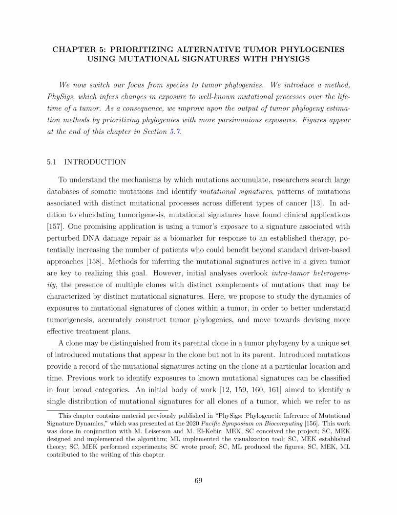
Chapter 5 then pivots into the context of tumor phylogeny estimation Here we propose

an approach that prioritizes alternative phylogenies inferred from the same sequencing data

using mutational signatures It was previously shown that distinct mutational processes

shape the genomes of the clones comprising a tumor These processes result in distinct mu-

tational patterns summarized by a small number of mutational signatures [12 13] Current

analyses of exposures to mutational signatures do not fully incorporate a tumorrsquos evolution-

ary context conversely current tumor phylogeny estimation methods do not incorporate

mutational signature exposures Here we introduce the Tree-constrained Exposure (TE)

problem to infer a small number of exposure shifts along the edges of a given tumor phy-

logeny Our algorithm PhySigs solves this problem and includes model selection to identify

the number of exposure shifts that best explain the data We validate our approach on

simulated data and identify exposure shifts in lung cancer data including at least one shift

with a matching subclonal driver mutation in the mismatch repair pathway When applying

PhySigs to the solution space T of plausible trees for a single patient we can then prioritize

the trees that have the fewest number of exposure shifts and are therefore more parsimonious

with respect to signature exposure We include an R package along with a tool to allow users

to visualize exposure shifts for various trees in a patient solution space

3

Chapter 4 likewise introduces a method for prioritizing the solution space for estimated

tumor phylogenies for a single patient tumor Rather than using mutational signatures here

we utilize sequencing data sourced from cohorts of patient tumors The idea is to leverage the

fact that tumors in different patients are the consequence of similar evolutionary processes

We wish to resolve ambiguities in our input data and detect subtypes of evolutionary patterns

by simultaneously (i) identifying a single tumor phylogeny among the solution space of

trees for each patient (ii) assigning patients to clusters and (iii) inferring a consensus tree

summarizing the identified expanded trees for each cluster of patients We formalize this as

the Multiple Choice Consensus Tree (MCCT) problem We show that this problem is NP-

hard via a reduction to 3-SAT and propose a gradient descent heuristic to use in practice

This framework addresses the limitations of previous work in that our problem statement

allows for different patient subtypes and our algorithm scales to larger sets of mutations

On simulated data we show that we are able to better recover the true patient trees and

patient clusters relative to existing approaches that do not account for patient subtypes

We then use RECAP to resolve ambiguities in patient trees and find repeated evolutionary

trajectories in lung and breast cancer cohorts

In summary this dissertation is structured as follows after introducing key background

material in Chapter 2 each chapter introduces a new method for improving phylogeny

estimation Chapter 3 introduces OCTAL a method for adding missing species into gene

trees using a reference tree Chapter 4 introduces TRACTION which builds on OCTAL

by using a reference tree to also correct low-support branches in gene trees The next two

chapters then shift to improving tumor phylogeny estimation Chapter 5 presents PhySigs a

method for improving tumor phylogeny estimation with mutational signatures and Chapter 6

presents RECAP a method for improving tumor phylogeny estimation using cohorts of

patient tumors Chapter 7 concludes with a discussion of future directions

4

CHAPTER 2 BACKGROUND

This chapter contains background material referenced throughout this dissertation Note

that key acronyms and terminology are defined once in this section rather than in each

subsequent chapter Sections 21ndash22 introduce species phylogenies and tumor phylogenies

respectively Each section begins with a discussion of the graph-theoretic objects before moving

on to current phylogeny estimation models and methods

21 SPECIES PHYLOGENY CONSTRUCTION

Species phylogenies are graphical objects used to represent the evolutionary relationship

between species as they have evolved through time Species phylogenies implicitly assume

that the represented species arise from a common ancestor and that genetic material is passed

down from parents to children along the branches of the tree Because this process happened

in the past phylogenies cannot be directly observed but instead must be estimated With

the advent of high throughput sequencing technology modern phylogeny estimation methods

leverage molecular sequence data sampled across species along with models of evolution to

reconstruct this history In this section we first introduce species phylogenies as a graphical

objects so as to define basic terminology Next we describe models of evolution under

which phylogenies are estimated and clarify the relationship between two subtypes of species

phylogenies gene trees estimated over a single locus and species trees estimated over the

whole genome1 Finally we discuss current methods for species phylogeny estimation along

with corresponding limitations

211 Species phylogenies as graph theoretic objects

A species phylogeny can be represented as a tree T with leaves labeled by a set S of

organisms If each leaf label is unique then the species phylogeny is singly-labeled Un-

less noted otherwise species phylogenies throughout this dissertation are singly-labeled and

unrooted

Rooted phylogenies Rooted trees offer an intuitive way to visualize evolution Indeed

since time is directed directed edges can be interpreted as capturing the passage of time

However estimates of species phylogenies are frequently unrooted because roots can be hard

1Note that we used the phrase ldquospecies phylogenyrdquo to refer to both gene and species tree estimation (wherethe leaves correspond to species) as a way to distinguish these trees from tumor phylogeny estimation

5

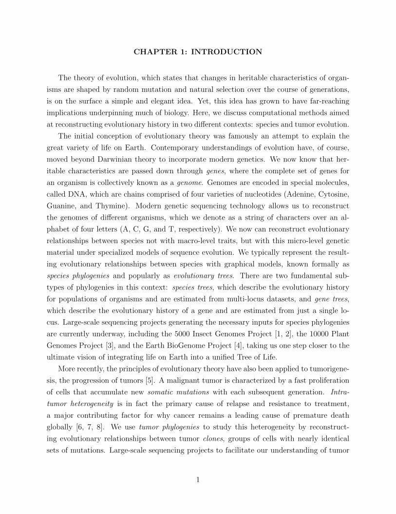
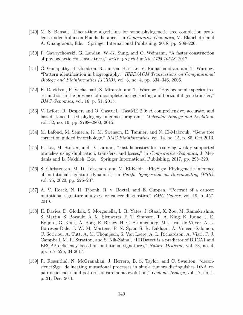
a b

Figure 21 Illustrative examples of the two types of phylogenies in this disserta-tion (a) Example of a rooted species phylogeny where the leaves represent extant species(b) Example of a tumor phylogeny where the leaves represent extant clones (ie cells sharinga common set of mutations) The colored circles denote the introduction of a new mutationdistinguishing a clone from its parent

to place (see [14] for a discussion) We introduce rooted trees here as a way to motivate the

unrooted species phylogenies we work with for the remainder of this dissertation

A rooted phylogeny can be represented as a rooted tree T with root vertex r If we direct

the edges of this tree away from the root then each vertex with the exception of r will

have an indegree of one When observing a directed edge from u to w between two vertices

uw in this tree we call u the parent of w Likewise w is the child of u We denote such an

edge with either urarr w or (uw) More broadly a vertex u is an ancestor of vertex w (and

conversely w is a descendant of u) if there exists a directed path from u to w If a vertex

does not have any children then it is considered to be a leaf Otherwise the vertex is an

internal node In practice leaves correspond to extant species and internal nodes correspond

to ancestral species Vertices with exactly two children are binary and vertices with more

than two children are polytomies A tree where each vertex is binary is called a binary tree

Given a subset of leaves R sube S in tree T a vertex is a common ancestor of R if it is an

ancestor of every leaf in R The common ancestor farthest from the root is known as the

most recent common ancestor (MRCA) or lowest common ancestor (LCA) of R A clade of

T is simply a subtree of T clades correspond to a subset of species defined by a common

ancestor and all descendants of that ancestor

6

Unrooted phylogenies A rooted species phylogeny can be converted into an unrooted

phylogeny by suppressing the orientation of the edges in the graph and removing any vertex

with degree two connecting its neighbors by a single undirected edge Each edge e in

an unrooted species phylogeny then defines a bipartition πe (also sometimes referred to as

a split) on the set of leaf labels induced by the deletion of e from the tree but not its

endpoints Each bipartition splits the leaf set into two non-empty disjoint parts A and

B and is denoted by A|B The set of bipartitions of a tree T is given by C(T ) = πe

e isin E(T ) where E(T ) is the edge set for T The leaves of an unrooted tree are vertices

with degree one and the remaining vertices are still considered internal nodes Notice that

without directed edges concepts like parent child and clade are no longer well-defined

Comparing unrooted phylogenies When working with species phylogenies it is im-

portant to have frameworks for comparing different trees Here we describe common re-

lationships between trees as well as define standard distances used to measure topological

similarity These distances may be deployed in the optimization problems used to construct

trees or in evaluating the accuracy of estimated trees when ground truth is known

We start by noting that trees are often restricted to the same set of leaves before making

a comparison More formally given a species phylogeny T on taxon set S T restricted to

R sube S is the minimal subgraph of T connecting elements of R and suppressing nodes of

degree two We denote this as T |R If T and T prime are two trees with R as the intersection

of their leaf sets their shared edges are edges whose bipartitions restricted to R are in the

set C(T |R) cap C(T prime|R) Correspondingly their unique edges are edges whose bipartitions

restricted to R are not in the set C(T |R) cap C(T prime|R)

We say that a tree T prime is a refinement of T if T can be obtained from T prime by contracting a

set of edges in E(T prime) A tree T is fully resolved (ie binary) if there is no tree that refines

T other than itself A set Y of bipartitions on some leaf set S is compatible if there exists

an unrooted tree T leaf-labeled by S such that Y sube C(T ) A bipartition π of a set S is

said to be compatible with a tree T with leaf set S if and only if there is a tree T prime such

that C(T prime) = C(T ) cup π (ie T prime is a refinement of T that includes the bipartition π)

Similarly two trees on the same leaf set are said to be compatible if they share a common

refinement An important result on compatibility is that pairwise compatibility of a set of

bipartitions over a leaf set ensures setwise compatibility [15 16] it then follows that two

trees are compatible if and only if the union of their sets of bipartitions is compatible

The Robinson-Foulds (RF) distance [11] between two trees T and T prime on the same leaf set is

defined as the minimum number of edge-contractions and refinements required to transform

T into T prime For singly-labeled trees the RF distance equals the number of bipartitions present

7

in only one tree (ie the symmetric difference) We define this formally as it is frequently

used in subsequent chapters

Definition 21 Given singly-labeled trees T and T prime both on leaf set S the Robinson-Foulds

distance is defined as

RF (T T prime) = |C(T ) C(T prime)|+ |C(T prime) C(T )| (21)

where C(T ) and C(T prime) are the sets of bipartitions in T and T prime respectively

The normalized RF distance is the RF distance divided by 2nminus6 where n is the number

of leaves in each tree this produces a value between 0 and 1 since the two trees can only

disagree with respect to internal edges and nminus 3 is the maximum number of internal edges

in an unrooted tree with n leaves

The matching distance [17] is another distance measure that relaxes the RF distance by

giving bipartitions forming a similar partition over the species set partial credit Formally

given two trees T and T prime on the same set of leaves we define a complete weighted bipartite

graph G = (C(T ) C(T prime) E) such that one set of vertices corresponds to bipartitions in T

and the other set corresponds to bipartitions in T prime The weight of an edge in G between

endpoints π isin C(T ) and πprime isin C(T prime) is the minimum hamming distance between any binary

vector encoding of each bipartition (ie consider an encoding and its complement) The

matching distance between T and T prime is then defined as the minimum weight perfect matching

on G Note that if the edge weights were instead binary with 0 for equal endpoints and 1

otherwise then the minimum weight perfect matching would equal the RF distance

A common measure that does not directly rely on bipartitions is the quartet distance

[18] A quartet is defined as the unrooted tree induced when restricting a tree to a subset

of four distinct leaves The quartet distance between two trees T and T prime on the same set of

leaves is then the number of four taxon subsets for which the quartet differs between trees

The motivation for using quartets is that they represent the smallest set of species for which

there is more than one possible unrooted tree topology (in fact there are three)

212 Gene and species trees

The precise interpretation of a species phylogeny can vary depending on the biological

context In particular there are two common subtypes of species phylogenies gene trees

and species trees Here we introduce these subtypes and discuss the underlying models of

evolution that give rise to this distinction

8

Gene trees In the context of this literature a gene is simply defined as a contiguous

subsequence of the genome (not necessarily coding for a protein) The evolutionary history of

a gene is then represented with a gene tree and estimated from genetic sequences descended

from some common ancestral gene This ancestral gene was passed down through many

generations ultimately arriving in the genomes of the individuals labeling the gene tree

leaves For the branching structure to hold gene trees must be estimated from regions of the

genome that are free of recombination [10] in other words the gene sequence was inherited

from one parent in every generation rather than intermixed between different individuals

As a gene replicates and its copies are passed on mutations or duplications may occur

that generate branching events in the gene tree When the leaves of a gene tree sample

individual representatives of different species leaves are either related via a speciation event

(orthologs) or via a duplication event (paralogs) (see discussion in [19]) The internal nodes

of the gene tree can be interpreted as corresponding to these ancestral events Note that

within a species individuals may have different versions of a gene referred to as alleles

Species trees We begin by acknowledging that there is not a definitive definition of a

species and delineating species is itself an area of research [20] for the purposes of develop-

ing computational methods we sidestep this issue by assuming that sequencing data from

distinct species has already been identified and provided as input

While a gene tree traces an individual gene lineage as it moves backwards in time a

species tree dictates the collection of potential ancestors from which a gene can be inherited

Branches of a species tree can be understood to contain generations of individuals when a

population becomes separated by speciation the genes within each nascent species likewise

become divided into two sets of lineages In this way gene trees are constrained by branches

of the species tree [10] Internal nodes of a species tree therefore correspond to speciation

events lineage-splitting that creates two or more separate species We typically expect

for an ancestral species to diverge into two descendant species creating a binary species

tree However there are some examples of ancient rapid radiation events these are short

periods of intense diversification that are especially hard to resolve creating polytomies in

the species tree [21] Unlike gene trees estimated from a single locus species trees incorporate

sequencing data from across the genome

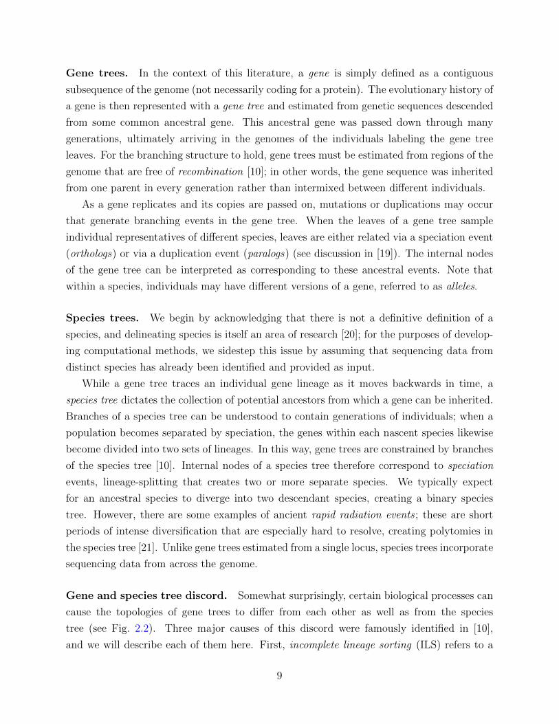
Gene and species tree discord Somewhat surprisingly certain biological processes can

cause the topologies of gene trees to differ from each other as well as from the species

tree (see Fig 22) Three major causes of this discord were famously identified in [10]

and we will describe each of them here First incomplete lineage sorting (ILS) refers to a

9

population-level phenomenon whereby gene lineages coalesce in a branch of the species tree

deeper than their MRCA When this happens the ordering of lineage merging may be such

that it differs from the species tree ILS is thought to be widespread and found across a

variety of species (eg [22 23 24]) Gene duplication and loss (GDL) refers to the process

whereby genes duplicate to create additional copies or are deleted during replication [25]

Complex patterns of duplication and loss can likewise lead to a gene tree that differs from

the species tree GDL has been observed in nature including between the human and great

ape [26] in fact gene duplication is thought to be a major driver of evolutionary change

as the duplicated gene takes on new functions (the orthologs conjecture) Finally reticulate

evolution describes the merging of ancestral lineages into a descendent lineage Examples

of reticulate evolution include hybridization [27] along with horizontal gene transfer (HGT)

[28] where an organism incorporates genetic information from a contemporary organism

other than its parent Reticulate evolution is well documented in bacteria and single cell

eukaryotes (eg [29 30 31 32]) but has also been observed in larger organisms such as

plants (eg [33 34 35])

There is a major conceptual difference between reticulate evolution as compared to ILS

and HGT The merging of branches in reticulate evolution results in a non-treelike process

and requires a more general graphical model called a phylogenetic network for proper anal-

ysis [36 37 38 39] However GDL and ILS produce heterogeneity across the genome that

can still be properly modeled by a single species tree [10 40] Species phylogeny estimation

methods should account for and be robust to this heterogeneity

Models relating gene and species trees Models of evolution allow us to establish

statistical relationships between gene and species trees as motivated above they are not

wholly independent Indeed a gene tree can be thought of as randomly drawn from the gene

tree distribution defined by a species tree Conversely a species tree can be inferred using

probabilistic models accounting for the distribution of gene trees induced by species trees

Much of the focus in the statistical phylogenetics literature has been on developing meth-

ods for species tree estimation in the presence of ILS which is modeled by the multi-species

coalescent (MSC) [41 42 43 44] Under the MSC model each branch of the species tree is

parameterized by the number of generations spanned by the branch and the size of the pop-

ulation contained in the branch (or twice that if species are diploid) These parameters are

the branch length and width respectively Since the probability that two lineages coalesce

on a branch is simply a function of length and width the parameterized species tree defines

a probability distribution over possible gene trees contained within its branches Species

trees with very short branches or very large populations are more likely to produce conflict-

10

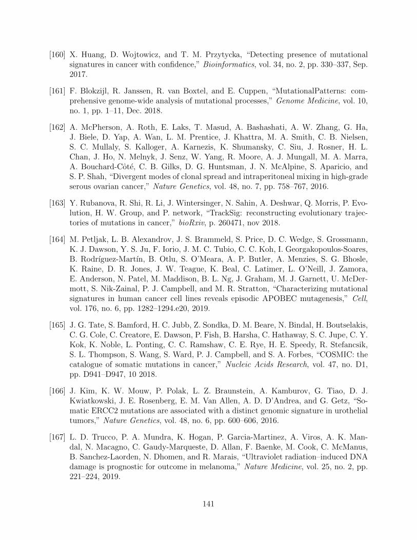
a b

Figure 22 Heterogeneity in modeling the evolution of single gene versus entiregenome (a) Examples of rooted gene trees which depict the evolutionary history of asingle gene for a collection of butterfly species Note that tree topologies may differ acrossgenes due to certain known biological phenomena such as GDL ILS and HGT (b) Exampleof a species tree which depicts the evolutionary history of the entire genome for a collectionof butterfly species Note that the species and gene tree topologies again may differ In somecases the species tree may not have the same topology as any gene tree

ing gene trees Under the MSC species trees are provably identifiable from the probability

distribution of gene tree topologies they define for certain models of sequence evolution [45]

There has been recent interest in expanding beyond MSC to model types of discord other

than ILS Notable examples of this include a probabilistic model accounting for just GDL

[46] followed by a unified model that accounts for both ILS and GDL [47]

Models of evolution are important to keep in mind when thinking about method assump-

tions and the data on which methods are tested Simplistic models of evolution can be more

computationally tractable but may for example suffer from being underspecified resulting

in a large solution space On the other hand highly parameterized methods may perform

well on data consistent with the model assumptions but may not be robust or transferable

to a wide range of datasets

213 Estimation methods

We now discuss existing approaches for both gene and species tree estimation While

the subsequent chapters of this dissertation primarily focus on improving gene trees we

introduce here how gene trees may be used as an input to estimate species trees In this

way improving gene tree estimation may improve species tree estimation albeit indirectly

11

Evaluating methods Computational methods must first and foremost perform well em-

pirically to be useful to biologists Since we do not typically know the ground truth on

real biological datasets simulated datasets are constructed under different models of evolu-

tion to benchmark method accuracy Researchers test methods under a range of conditions

evaluating robustness to error model misspecification and challenging edge cases

It is likewise important to establish the theoretical proprieties of each method For

instance there is a lot of interest in showing methods are statistically consistent that is

error in the estimated model parameters provably goes to zero as the amount of input

data generated under the model approaches infinity Otherwise the method is said to be

statistically inconsistent While statistical consistency is important it is worth reiterating

that it only describes performance at the limit In practice methods are run on finite data

which statistical consistency does not address Another important theoretical consideration

is time complexity which indicates the scalability of a method to large datasets with many

species Algorithms will need to accommodate large-scale sequencing projects underway

such as the 5000 Insect Genomes Project [1 2] the 10000 Plant Genomes Project [3] and

the Earth BioGenome Project whose goal is to sequence 15 million eukaryotic species [4]

Gene tree estimation The input to gene tree estimation methods is typically a multiple

sequence alignment (MSA) for the gene of interest across a set of species An alignment

can be represented as a matrix where each row contains the genomic sequence for a species

interspliced with gap character states gaps are introduced so as to ensure that characters

in the same column are homologous meaning they evolved from the same nucleotide in

a common ancestor MSAs are an active area of research and beyond the scope of this

dissertation we refer the interested reader to the chapter on MSA in [48]

Given an MSA there are broadly two types of approaches for estimating a gene tree

Non-statistical approaches include constructing trees from qualitative characters (eg max-

imum parsimony and maximum compatibility) and certain types of distance methods (eg

neighbor joining) Statistical approaches on the other hand explicitly account for mod-

els of evolution Examples of these approaches include maximum likelihood and Bayesian

methods Across methods there are different trade-offs some are heuristics for NP-hard

problems some are computationally intensive some lack certain theoretical properties such

as statistical consistency However one limitation that all these methods have in common is

that gene tree estimation based on a single locus is more susceptible to (1) missing sequenc-

ing data for that gene for certain species and (2) not containing enough signal to determine

the correct gene tree topology with high confidence (see Chapter 1 and discussion in [49 50])

One approach from the GDL literature to address limited signal is to modify estimated

12

gene trees with respect to a reference tree which may either be an established tree from

prior studies or an estimated species tree (eg based on an assembled multi-gene dataset)

Such methods are typically based on parametric models of gene evolution and broadly fall

into two categories Integrative methods use available sequence data in addition to the

estimated gene tree and reference tree examples include ProfileNJ [51] TreeFix [52] and

TreeFix-DTL [53] On the other hand gene tree correction methods only use the gene

tree and species tree topologies Notung [54 55] and ecceTERA [56] are two well-known

methods of this type Integrative methods are generally expected to be more accurate than

gene tree correction methods in the presence of GDL but are also more computationally

intensive as a result of performing likelihood calculations with the sequencing data See

[57 58 59 60 61 62] for additional literature on this subject We build on this line of work

in Chapters 3-4 by introducing non-parametric approaches for gene tree correction that can

be used in contexts outside of GDL such as ILS and HGT

Species tree estimation A straightforward approach for estimating species trees is sim-

ply to concatenate together a multi-locus dataset and then run a method described above

on the resulting alignment Such an approach is often referred to as concatenation and is

indeed quite popular [63 64] Despite competitive empirical performance on benchmark

experiments [65] these methods tend to suffer from a number of theoretical limitations

For example one of the most common versions of concatenation uses maximum likelihood

(CA-ML) Under the simplest unpartitioned version of CA-ML all loci are assumed to evolve

down a single model tree an assumption that is violated when recombination occurs between

loci Furthermore it was shown that unpartitioned CA-ML is statistically inconsistent and

sometimes positively misleading under the MSC model [44]

Another intuitive approach for estimating species trees from multi-locus data is to first

estimate gene trees and then combine them into a species tree leveraging the fact that

the two types of trees are related The simplest way to combine them is to use the most

frequent gene tree topology as the estimate of the species tree This approach has been proven

statistically consistent under the MSC for rooted species trees with three leaves or unrooted

trees with four leaves but not when more leaves are present [66 67 68 69] However there

are related approaches that combine gene trees into a larger species tree in a way that is

statistically consistent under the MSC model Some of these summary methods such as

ASTRAL-II [70] and ASTRID [71] have been shown to scale well to datasets with many

taxa (ie gt1000 species) and provide accurate species tree estimates Note that summary

methods have many features in common with supertree methods that combine source trees

on overlapping leaf sets (see discussion in [72]) but are based on mathematical properties

13

of the MSC model and so can be proven statistically consistent under this model supertree

methods by contrast assume conflict between source trees is due to estimation error rather

than ILS and so are generally not statistically consistent under the MSC model

Finally there also exist co-estimation methods that indirectly rely on gene trees These

methods work by taking as input an MSA and then inferring gene and species trees together

[73] While these methods are often computationally expensive the approach supports the

idea that species and gene trees may be able to improve one another iteratively

22 TUMOR PHYLOGENY CONSTRUCTION

We now switch our attention from species phylogenies to tumor phylogenies Tumor

phylogeny estimation is a related but distinct conceptual challenge from species phylogeny

estimation Many of these differences stem from the fact that evolution is happening at a

different scale where the leaves of the phylogeny are not known a priori

Tumors develop via an evolutionary process [5] tumor cells rapidly grow and divide ac-

quiring new mutations with each subsequent generation Mutations that accumulate during

the lifetime of an individual are referred to as somatic mutations as opposed to germline

mutations that are inherited Under the infinite sites assumption (ISA) each mutation is

gained exactly once and never lost giving rise to a two-state perfect phylogeny The ISA

underlies the majority of current methods for tumor phylogeny inference from both bulk

and single-cell DNA sequencing data (reviewed in [74]) In line with this work we likewise

adhere to the ISA unless it is noted otherwise we acknowledge that this is a simplifying

assumption that should be relaxed in future work

221 Tumor phylogenies as graph theoretic objects

We begin by reviewing the basic graphical objects underlying tumor phylogenies Note

that we hold off on diving into tumor biology until the next section as a consequence certain

terms like mutation are left intentionally vague

Rooted phylogenies The evolutionary history of n mutations of a tumor is represented

by a particular type of rooted tree T whose root vertex is denoted by r(T ) vertex set by V (T )

and directed edge set by E(T ) Similar to the rooted species phylogenies introduced above

the edges of a tumor phylogeny are directed away from the root The terms parent child

ancestor and descendant are used in an analogous fashion when describing the relationship

14

119879 119879119879

119879$ 119879 119879amp

Figure 23 Unlike a species phylogeny leaves of a tumor phylogeny are not knowna priori (Left) Two different species phylogenies TA TB with the same set of species labelingthe leaves (Right) Four different tumor phylogenies that differ in distinct ways Trees T1

and T2 have the same set of clones labeling the leaves but a different ancestral relationshipbetween the mutations on the right branch Trees T1 and T3 have the same set of mutationsbut different clones Trees T1 and T4 have different mutations and different clones

between two vertices Other general tree terminology also carries over directly including

binary polytomy common ancestor and most recent common ancestor

The vertices of T now represent groups of cells or clones that have nearly identical

mutational profiles The leaves of T correspond to the extant clones present at the time of

sampling and the internal nodes correspond to ancestral clones in the tumor Under the

ISA mutations are gained once and never lost Thus each mutation is present on exactly one

edge of T and we may label each non-root vertex v 6= r(T ) by the mutations micro(v) = micro(u v)

introduced on its unique incoming edge (u v) The root vertex r(T ) typically corresponds

to the normal or non-mutated clone and is represented by the empty set micro(r(T )) = emptyIf more than one mutation is gained on an edge then we call the child vertex v a mutation

cluster (ie |micro(v)| gt 1) Such mutation clusters represent a type of ambiguity where the

linear ordering of mutation gain is unknown We say that a tree T prime is an expansion of a tree

T if all mutation clusters of T have been expanded into ordered paths such that only one

mutation is gained on each edge In particular for a mutation cluster with n mutations there

are n possible expanded paths We also define the ancestral set A(v) of vertex v as the set

of mutations that label the path from r(T ) to v in T A(v) defines the full set of mutations

15

Figure 24 Three different distance measures for comparing tumor phylogeniesEach measure takes the symmetric difference between sets from each tree Clonal distanceuses the set of clones parent-child distance uses the set of directed edges and ancestor-descendant distance uses the set of all ancestor-descendant mutation pairs Here we com-pute each distance between trees T1 and T2 We show the elements contributing to thesymmetric difference in each case Items in T1 but not T2 are shown in the column on theleft Conversely items in T2 but not T1 are shown in the right column

present in the clone represented by v We say that two edges (u v) isin E(T ) (uprime vprime) isin E(T prime)

are equal if they have the same set of mutations present at their corresponding endpoints

(ie micro(u) = micro(uprime) micro(v) = micro(vprime))

Comparing rooted phylogenies There are several reasons why the methods for com-

paring rooted species phylogenies do not immediately translate to tumor phylogenies The

first reason is that the leaves of a tumor tree are not known a priori we typically observe

the set of mutations for a patient but the clustering of these mutations into clones is not

directly observed This creates scenarios where even for a fixed set of mutations we may

want to compare alternative tumor phylogenies with different clones A second reason is

that there is only one tree of life but there are many separate instances of tumor evolution

occurring in different patient tumors Here we may want to compare trees not only with

different clones but also with different sets of mutations In other words tumor comparisons

must operate at the level of the mutation sets labeling each vertex rather than collapsing

these sets into some higher order notion of species (see Fig 24)

Recall that above we introduced the notion of RF distance between unrooted species

phylogenies In the rooted setting RF distance can be modified slightly to equal the sym-

metric difference of the sets of clades rather than bipartitions In an attempt to adapt this

to tumor phylogenies we could think of a clade as being represented by the set of mutations

gained within that clade However there is something flawed with this approach working

16

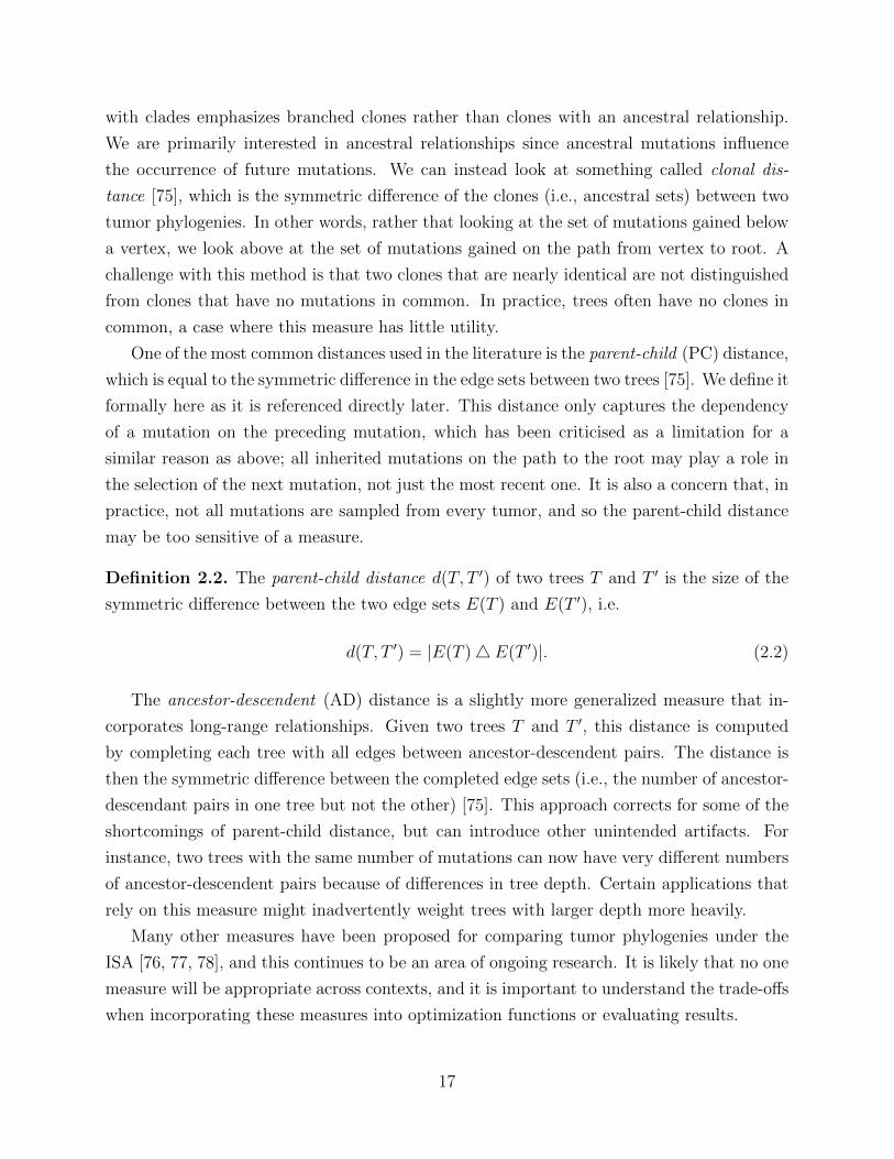
with clades emphasizes branched clones rather than clones with an ancestral relationship

We are primarily interested in ancestral relationships since ancestral mutations influence

the occurrence of future mutations We can instead look at something called clonal dis-

tance [75] which is the symmetric difference of the clones (ie ancestral sets) between two

tumor phylogenies In other words rather that looking at the set of mutations gained below

a vertex we look above at the set of mutations gained on the path from vertex to root A

challenge with this method is that two clones that are nearly identical are not distinguished

from clones that have no mutations in common In practice trees often have no clones in

common a case where this measure has little utility

One of the most common distances used in the literature is the parent-child (PC) distance

which is equal to the symmetric difference in the edge sets between two trees [75] We define it

formally here as it is referenced directly later This distance only captures the dependency

of a mutation on the preceding mutation which has been criticised as a limitation for a

similar reason as above all inherited mutations on the path to the root may play a role in

the selection of the next mutation not just the most recent one It is also a concern that in

practice not all mutations are sampled from every tumor and so the parent-child distance

may be too sensitive of a measure

Definition 22 The parent-child distance d(T T prime) of two trees T and T prime is the size of the

symmetric difference between the two edge sets E(T ) and E(T prime) ie

d(T T prime) = |E(T )4 E(T prime)| (22)

The ancestor-descendent (AD) distance is a slightly more generalized measure that in-

corporates long-range relationships Given two trees T and T prime this distance is computed

by completing each tree with all edges between ancestor-descendent pairs The distance is

then the symmetric difference between the completed edge sets (ie the number of ancestor-

descendant pairs in one tree but not the other) [75] This approach corrects for some of the

shortcomings of parent-child distance but can introduce other unintended artifacts For

instance two trees with the same number of mutations can now have very different numbers

of ancestor-descendent pairs because of differences in tree depth Certain applications that

rely on this measure might inadvertently weight trees with larger depth more heavily

Many other measures have been proposed for comparing tumor phylogenies under the

ISA [76 77 78] and this continues to be an area of ongoing research It is likely that no one

measure will be appropriate across contexts and it is important to understand the trade-offs

when incorporating these measures into optimization functions or evaluating results

17

222 Clonal theory of evolution

The landmark paper by Nowell [5] posits that cancer results from an evolutionary process

whereby cells within a tumor descend from a single founder cell As cells grow and divide

new mutations are introduced leading to genetically-distinct subpopulations of cells known as

clones Clones are subject to selective pressure exerted by surrounding tissues the immune

system and treatments Particularly advantageous combinations of mutations are selected

for and create clonal expansions where many copies of a particular clone arise in a tumor

Types of somatic mutations Genetic variation observed in cancer can be classified

into different types depending on the scale in which it operates Small-scale variations

(lt 1 kilobase in length) include insertions and deletions as well as point mutations We

note that when germline point mutations are common to a population they are referred to

as single nucleotide polymorphisms (SNPs) This is not to be confused with somatic point

mutations arising in tumor cells which are referred to as single nucleotide variants (SNVs)

On the other hand large-scale variations (gt 1 kilobase in length) include chromosomal

rearrangements (eg translocation transversion segmental) and copy number aberrations

(CNAs) such as gain or loss At the largest scale there can be variation in the number of

whole chromosomes or genomes (eg polyploidy aneuploidy)

Models of tumor evolution Much of the current work in tumor phylogenetics focuses

on just SNVs and relies on the ISA Recall under the ISA each mutation can only be gained

once and never lost In the two-state case this corresponds to a tree where the root vertex

starts with state 0 (non-mutated) for each character Each character can change state from

0 to 1 only once in the tree but never revert back This model is known as the two-state

perfect phylogeny model A more general version has also been proposed called the multi-

state perfect phylogeny model which likewise prohibits homoplasy A character in this model

can change states more than once but never change back to a previous state

SNVs and CNAs can interact in such a way that reliably violates the standard ISA

assumption making the two-state perfect phylogeny model unrealistic For instance a copy

number deletion that overlaps with an SNV causes a loss of that SNV in descendent cells

One straightforward solution that is often deployed is to exclude all SNVs that occur in

regions where a CNA has been detected However aneuploidy drives extensive CNAs in

approximately 90 of tumors [79 80] removing these regions results in a major loss of data

More general models of evolution have been proposed in response to these concerns While

the methods in this dissertation are primarily developed under ISA we include these models

18

because they are an important direction of future research

Under the Dollo parsimony model [81] a mutation can be gained only once but it can

be lost multiple times A variation on this model is the k-Dollo parsimony model which

restricts each mutation to being lost at most k times [82] Because the loss of SNVs due to

CNAs is much more prevalent than gaining the same mutation twice via parallel evolution

this relaxation captures dominant factors underlying the evolution of SNVs in cancer

The finite sites model is even more general allowing for parallel evolution along with

mutation loss This is a parameterized model that uses a continuous-time Markov chain

to assign probabilities along branches of the tumor phylogeny for each possible transition

between a homozygous reference or a heterozygous or homozygous non-reference genotype

The model assumes that each site in the genome evolves identically and independently

through time Thus a major conceptual limitation of both this and the Dollo model is that

although they allow for loss they do not consider CNAs that produce loss dependencies

across sites Recent work [83] has tried to address this concern by using a loss-supported

phylogeny model which constrains losses to regions with evidence of copy number decrease

Hallmarks of cancer While each tumor results from a different instantiation of this

evolutionary process it is postulated that the complexity of all cancers can be reduced

to a small number of principles so called hallmarks of cancer [84 85] The theory states

that normal cells must obtain a certain set of traits such as ldquoevading growth suppressorsrdquo

ldquoresisting cell deathrdquo and ldquoenabling replicative immortalityrdquo to eventually turn malignant

The increasing availability of tumor sequencing data has led to the use of phylogenies to

identify driver mutations interfering with genes or pathways potentially linked to these

common traits driving cancer progression [86 87]

Driver mutations in turn may then be used to identify repeated evolutionary trajectories

in tumorigenesis and metastasis [88 89 90 91] Crucially it has been suggested that the

co-occurrence and ordering rather than just mutation presence have significant prognostic

consequences as was shown for example in a study of myeloproliferative neoplasms with

the ordering of JAK2 and TET2 mutations [92] Early methods for revealing evolutionary

trajectories from cohorts of patients find evidence of reoccuring patterns but suffer from

scalability issues and make simplifying assumptions about patient subtypes [90 91] It is the

hope that identifying patient subtypes with shared evolutionary patterns called evolutionary

subtypes will eventually lead to clinically-relevant subtypes enabling precision medicine

Nevertheless there is an exponential number of orderings in which these mutations can be

acquired and identifying these hallmarks remains a great challenge We address this issue

further in the final chapter of this dissertation

19

223 Estimation methods

Tumor phylogeny estimation methods have been developed for a range of sequencing

technologies However most current methods only reconstruct the evolutionary history of

SNVs with some methods also accounting for changes in copy number [82 93 94] We focus

on such methods here unless otherwise noted Future methods will need to account for the

other types of structural variation that can occur in the genome

Bulk sequencing The majority of patient tumor data is currently obtained via bulk DNA

sequencing For instance almost all datasets from The Cancer Genome Atlas (TCGA) and

International Cancer Genome Consortium (ICGC) consist of single bulk tumor samples

The input to bulk sequencing is a mixed sample of short reads (lt 300 bp) taken from

potentially millions of cells with varying genomes [95 96] In practice samples will not

just contain tumor cells but also normal cells The fraction of tumor cells in a sample is

known as the purity Reads are then aligned to a reference genome For each SNV present

in a bulk sample we directly observe the fraction of DNA sequencing reads aligned to that

location in the genome containing a variant allele This fraction is the variant allele frequency

(VAF) and the denominator (ie the number of aligned reads) is the read depth The VAF

estimates the fraction of tumor chromosomes containing an SNV with some error introduced

by the stochasticity of sequencing Note that this is not the same as the fraction of cells

containing an SNV known as the cancer cell fraction (CCF) as purity and copy number

obscure the relationship However VAF can be assumed as proportionate to CCF under

the ISA if CNAs are ignored since this implies all mutated cells are heterozygous diploid

Alternatively several methods have been developed to use copy number to more carefully

convert VAF into CCF [97] Tumor phylogeny estimations methods then use VAF or CCF to

simultaneously identify the clones and tree topology over these clones (see [74] for a survey)

Methods here are inherently trying to solve a mixture problem intuitively we have as

input a matrix F where the rows correspond to tumor samples and columns correspond

to mutations The entries of this matrix are the proportion of cells containing a mutation

in a sample Informally the objective is to factorize F into (1) a matrix B specifying the

clustering of mutations into clones and (2) a mixture matrix U describing the proportion of

clones in each sample When additional constraints are placed on B so that the clones are

consistent with an evolutionary model we call it a phylogeny mixture problem Much work

has been done on studying the Perfect Phylogeny Mixture (PPM) problem [98] where the

evolutionary model placed on B is the two-state perfect phylogeny (ie B must correspond

to a perfect phylogeny) Deciding if such a factorization of F into UB exists in this setting

20

has been shown to be NP-complete [98] Minimizing the factorization error or sampling from

the solution space is therefore NP-hard note that the solution is not necessarily unique [99]

Several heuristic methods have been developed that try to solve variations of this mixture

problem in practice Methods that specialize in estimating tumor phylogenies from just one

bulk sample typically need to make additional strong assumptions such as strong parsimony

or sparsity [100] because one sample does not provide sufficient constraint Fortunately as

sequencing has become cheaper and more pervasive there has been a rise in bulk sequencing

studies that collect multiple samples from the same tumor either spatially (eg [87 101

102 103]) or temporally (eg [89 104]) This has led to a boon in multi-sample bulk

sequencing methods some of which just model SNVs and others that also account for CNAs

[98 105 106 107 108] A method has also been proposed that moves beyond two-state

and assumes the multi-state perfect phylogeny model [109] A current limitation shared by

all of these methods is that they do not infer a single tree per patient but rather a large

solution space of plausible trees for each individual patient [95 96] Identifying the true tree

is important to effective downstream analysis either additional data must be collected or

additional constraints should be explored in order to select one tree for each patient

Single cell sequencing Single-cell sequencing allows us to directly observe specific cells

present within a tumor without deconvolution While promising single-cell sequencing is

currently expensive and not performed at scale Moreover the data suffers from a number of

technical challenges that must be adequately addressed These sequences are known to have

elevated rates of false positives and negatives from genome amplification as well as significant

amounts of missing data since only a small fraction of tumor cells are sequenced [110 111]

This is especially problematic in the context of cancer where it is hard to determine if a

variant is a subclonal mutation or an error While early single cell methods directly applied

classic phylogeny estimation techniques like neighbor joining [112] more recent methods

have tried to explicitly model the single cell sequencing errors for better results [77 82 93

113 114] Still single cell methods have some limitations especially in establishing linear

mutation orderings due to high noise levels and missing ancestral clones [115]

Some methods look to combine single cell and bulk sequencing data in a complementary

way to overcome the limitations of each technology [115] For example bulk sequencing is

an inexpensive way to generate a set of plausible tumor phylogenies for a patient Targeted

single cell sequencing can then be used to rule out phylogenies and hopefully select the true

tree [116] While this is again another promising direction such combined datasets are rare

and require the ability to do additional sequencing Later we look to see what signal we

can extract from existing datasets when additional sequencing is not an option

21

CHAPTER 3 CORRECTING GENE TREES TO INCLUDE MISSINGSPECIES USING A REFERENCE TREE WITH OCTAL

We begin the main body of this dissertation with a method for adding missing species into

gene trees using a reference tree This reference tree is typically estimated from a multi-locus

dataset and used as a surrogate in the case where sequencing information is missing for the

gene of interest Figures and tables appear at the end of this chapter in Section 36

31 INTRODUCTION

A common challenge for phylogeny estimation methods is that sequence data may not

be available for all genes and species of interest creating conditions with missing data

[49 50 119] Gene trees can be missing species simply because some species do not contain

a particular gene and in some cases no common gene will be shared by every species in the

set of taxa [120] Additionally not all genomes may be fully sequenced and assembled as

this can be operationally difficult and expensive [50 121]

Missing gene data has both practical and theoretical implications the impact of which

may propagate into downstream analysis including species tree estimation Although species

tree summary methods are statistically consistent under the MSC model [122] the proofs

of statistical consistency assume that all gene trees are complete and so may not apply

when the gene trees are missing taxa Recent extensions to this theory have postulated

that some species tree estimation methods are statistically consistent under some models of

missing data (eg when every species is missing from each gene with uniform probability)

[123 124 125] However missing data in biological datasets often violates such models [119]

for example missing data may be biased towards genes with faster rates of evolution [126]

Furthermore sparse multi-locus datasets can be phylogenetically indecisive meaning more

than one tree topology can be optimal making it impossible to distinguish between multiple

alternative trees [127] Because of concerns that missing data may reduce the accuracy

of multi-locus species tree estimation methods many phylogenomic studies have restricted

their analyses to only include genes with most of the species (see discussion in [49 50 128])

We address this challenge by adding missing species back into gene trees using auxiliary

This chapter contains material previously presented at the 2017Workshop on Algorithms in Bioinfor-matics [117] and later published in Algorithms for Molecular Biology under the title ldquoOCTAL OptimalCompletion of Gene Trees in Polynomial Timerdquo [118] This work was done in conjunction with EK Mol-loy P Vachaspati and T Warnow TW conceived the project PV EKM designed and implemented thealgorithm SC EKM TW established theory SC TW wrote proofs SC PV EKM performed experimentsSC EKM produced the figures SC EKM TW contributed to the writing of this chapter

22

information from other regions of the genome In doing so we formulate the Optimal Tree

Completion (OTC) problem which seeks to add missing species to a gene tree so as to mini-

mize distance to another tree called a reference tree In this chapter we specifically address

the Robinson-Foulds (RF) Optimal Completion problem which seeks a completion that

minimizes the RF distance between the two trees We then present the Optimal Completion

of Incomplete gene Tree Algorithm (OCTAL) a greedy polynomial time algorithm that we

prove solves the RF Optimal Completion problem exactly We also present results from an

experimental study on simulated datasets comparing OCTAL to a heuristic for gene tree

completion within ASTRAL-II

32 PROBLEM STATEMENT

The problem we address in this paper seeks to add leaves into an incomplete tree in such

a way as to minimize distance to an existing tree where the distance between trees is defined

by the RF distance (see Def 21) A formal statement of the problem is as follows

Problem 31 (RF Optimal Tree Completion (RF-OTC)) Given an unrooted binary

tree T on the full taxon set S and an unrooted binary tree t on a subset of taxa R sube S

output an unrooted binary tree T prime on the full taxon set S with two key properties

1 T prime is a S-completion of t (ie T prime contains all the leaves of S and T prime|R = t) and

2 T prime minimizes the RF distance to T among all S-completions of t

Note that t and T |R are both on taxon set R but need not be identical In fact the RF

distance between these two trees is a lower bound on the RF distance between T and T prime

33 METHODS

In this section we present OCTAL an algorithm for solving the RF-OTC problem exactly

in polynomial time The algorithm begins with input tree t and adds leaves one at a time

from the set S R until a tree on the full set of taxa S is obtained To add the first leaf

we choose an arbitrary taxon x to add from the set S R We root the tree T |Rcupx (ie T

restricted to the leaf set of t plus the new leaf being added) at x and then remove x and the

incident edge this produces a rooted binary tree we will refer to as T (x) that has leaf set R

We perform a depth-first traversal down T (x) until a shared edge e (ie an edge where

the clade below it appears in tree t) is found Since every edge incident with a leaf in T (x)

23

Figure 31 One iteration of the OCTAL algorithm Trees T and t with edges in thebackbone (defined to be the edges on paths between nodes in the common leaf set) coloredgreen for shared and blue for unique all other edges are colored black After rooting T |Rwith respect to u the edges in T |R that could be identified by the algorithm for ldquoplacementrdquoare indicated with an asterisk () Note that any path in T |R from the root to a leaf willencounter a shared edge since the edges incident with leaves are always shared In thisscenario the edge e above the least common ancestor of leaves w and x is selected this edgedefines the same bipartition as edge eprime in t Hence AddLeaf will insert leaf u into t bysubdividing edge eprime and making u adjacent to the newly added node

is a shared edge every path from the root of T (x) to a leaf has a distinct first edge e that is

a shared edge Hence the other edges on the path from the root to e are unique edges

After we identify the shared edge e in T (x) we identify the edge eprime in t defining the same

bipartition and we add a new node v(eprime) into t so that we subdivide eprime We then make x

adjacent to v(eprime) Note that since t is binary the modification tprime of t that is produced by

adding x is also binary and that tprime|R = t These steps are then repeated until all leaves from

S R are added to t This process is shown in Figure 31 and given in Algorithm 31 below

331 Proof of Correctness

Let T be an arbitrary binary tree on taxon set S and t be an arbitrary binary tree

on taxon set R sube S Let T prime denote the tree returned by OCTAL given T and t We set

r = RF (T |R t) As we have noted OCTAL returns a binary tree T prime that is an S-completion

of t Hence to prove that OCTAL solves the RF Optimal Tree Completion problem exactly

we only need to establish that RF (T T prime) is the smallest possible of all binary trees on leaf

set S that are S-completions of t While the algorithm works by adding a single leaf at a

time we use two types of subtrees denoted as superleaves to aid in the proof of correctness

Definition 31 The backbone of T with respect to t is the set of edges in T that are on a

path between two leaves in R

Definition 32 A superleaf of T with respect t is a rooted group of leaves from S R that

is attached to an edge in the backbone of T In particular each superleaf is rooted at the

24

Algorithm 31 RF Optimal Tree Completion Algorithm (OCTAL)

Input Binary tree t on taxon set R sube S binary tree T on taxon set SOutput Binary tree tprime on taxon set S solving the RF-OTC problem

Function AddLeafRoot T2 at v the neighbor of x and delete x to get a rooted version of T2|KPick arbitrary leaf y in T2|K and find first edge e isin E on path from v to yFind eprime in T1 defining the same bipartition as eAttach x to eprime in T1 by subdividing eprime and making x adjacent to the newlycreated node call the resulting tree T prime1

return T prime1

Function Mainif R=S then

return telse

E larr Preprocess and initialize set of shared edges between t and T |RRprime larr R Initialize Rprime by setting it equal to input Rtprime larr t Initialize tprime by setting it equal to input tfor x isin S rR do

Rprime larr Rprime cup xT prime larr T |Rprime

tprime larr AddLeaf(x tprime T prime E)E larr Update shared edges between tprime and T prime

endreturn tprime

end

node that is incident to one of the edges in the backbone

Definition 33 There are exactly two types of superleaves Type I and Type II

1 A superleaf is a Type I superleaf if the edge e in the backbone to which the superleaf is

attached is a shared edge in T |R and t It follows then that a superleaf X is a Type I

superleaf if and only if there exists a bipartition A|B in C(t)capC(T |R) where A|(BcupX)

and (A cupX)|B are both in C(T |RcupX)

2 A superleaf is a Type II superleaf if the edge e in the backbone to which the superleaf

is attached is a unique edge in T |R and t It follows that a superleaf X is a Type II

superleaf if and only if for any bipartition A|B such that A|(B cup X) and (A cup X)|Bare both in C(T |RcupX) A|B 6isin C(t)

Now we begin our proof by establishing a lower bound on the RF distance to T for all

binary S-completions of t

25

Lemma 31 Let Y be a Type II superleaf for the pair (T t) and let x isin S R Let tlowast be

the result of adding x into t arbitrarily (ie we do not attempt to minimize the resulting

RF distance) If x 6isin Y then Y is a Type II superleaf for the pair (T tlowast) Furthermore if

x isin Y then RF (T |Rcupx tlowast) ge RF (T |R t) + 2

Proof It is easy to see that if x 6isin Y then Y remains a Type II superleaf after x is added

to t Now suppose x isin Y We will show that we cannot add x into t without increasing the

RF distance by at least 2 Since Y is a Type II superleaf it is attached to a unique edge

in T |RcupY and this is the same edge that x is attached to in T |Rcupx So suppose that x is

added to t by subdividing an arbitrary edge eprime in t with bipartition C|D note that we do not

require that x is added to a shared edge in t After adding x to t we obtain tree tlowast whose

bipartition set includes C|(D cup x) and (C cup x)|D If C|D corresponds to a unique edge

relative to t and T |R then both of these bipartitions correspond to unique edges relative

to tlowast and T |Rcupx If C|D corresponds to a shared edge then at most one of the two new

bipartitions can correspond to a shared edge as otherwise we can derive that Y is a Type I

superleaf Hence the number of unique edges in t must increase by at least one no matter

how we add x to t where x belongs to a Type II superleaf Since t is binary the tree that

is created by adding x is binary so that RF (T |Rcupx tlowast) ge RF (T |R t) + 2 QED

Lemma 32 Let T lowast be an unrooted binary tree that is a S-completion of t Then we have

RF (T lowast T ) ge r+ 2m where r = RF (T |R t) and m is the number of Type II superleaves for

the pair (T t)

Proof We note that adding a leaf can never reduce the total RF distance The proof follows

from Lemma 31 by induction QED

Now that we have established a lower bound on the best achievable RF distance (ie

the optimality criterion for the RF Optimal Tree Completion problem) we show OCTAL

outputs a tree T prime that is guaranteed to achieve this lower bound We begin by noting that

when we add x to t by subdividing some edge eprime creating a new tree tprime all the edges other

than eprime in t continue to ldquoexistrdquo in tprime although they define new bipartitions In addition eprime

is split into two edges which can be considered new Thus we can consider whether edges

that are shared between t and T remain shared after x is added to t

Lemma 33 Let tprime be the tree created by AddLeaf given input tree t on leaf set R and

tree T on leaf set Rcupx If x is added to tree t by subdividing edge eprime to create tprime then all

edges in t other than eprime that are shared between t and T remain shared between tprime and T

26

Proof Let T (x) be the rooted tree obtained by rooting T at x and then deleting x Let e be

the edge in T (x) corresponding to eprime and let πe = A|B without loss of generality assume A

is a clade in T (x) Note that C(T ) contains bipartition A|(Bcupx) (however C(T ) may not

contain (A cup x)|B unless e is incident with the root of T (x)) Furthermore for subclade

Aprime sube A Aprime|(R Aprime) isin C(T |R) and Aprime|(R Aprime cup x) isin C(T ) Now suppose elowast in t is a

shared edge between t and T |R that defines bipartition C|D 6= A|B Since A|B and C|Dare both bipartitions of t without loss of generality either C sub A or A sub C If C sub A then

C is a clade in T (x) and so elowast defines bipartition C|(D cup x) within tprime But since C sub A

the previous analysis shows that C|(D cup x) is also a bipartition of T and so elowast is shared

between T and tprime Alternatively suppose A sub C Then within tprime elowast defines bipartition

(C cup x)|D which also appears as a bipartition in T Hence elowast is also shared between T

and tprime Therefore any edge elowast other than eprime that is shared between t and T remains shared

between tprime and T for all leaves x added by AddLeaf QED

Lemma 34 OCTAL(T t) preserves the topology of superleaves in T In other words for

any superleaf with leaves Q sube S OCTAL(T t)|Q equals T |Q

Proof We will show this by induction on the number of leaves added The lemma is trivially

true for the base case when just one leaf is added to t Let the inductive hypothesis be that

the lemma holds for adding up to n leaves to t for some arbitrary n isin N+ Now consider

adding n + 1 leaves and choose an arbitrary subset of n leaves to add to t creating an

intermediate tree tprime on leaf set K using the algorithm OCTAL Let x be the next additional

leaf to be added by OCTAL

If x is the first element of a new superleaf to be added it is trivially true that the topology

of its superleaf is preserved but we need to show that x will not break the monophyly of an

existing superleaf in tprime By the inductive hypothesis the topology of each superleaf already

placed in tprime has been preserved Thus each superleaf placed in tprime has some shared edge

in tprime and T |K incident to that superleaf If x were placed onto an edge contained in some

existing superleaf that edge would change its status from being shared to being unique

which contradicts Lemma 33

The last case is where x is part of a superleaf for the pair (T t) that already has been

partially added to t AddLeaf roots T |Kcupx at x and removes the edge incident to x

creating rooted tree T (x) The edge incident to the root in T (x) must be a shared edge by

the inductive hypothesis Thus OCTAL adds x to this shared edge preserving the superleaf

topology QED

Lemma 35 OCTAL(T t) returns binary tree T prime such that RF (T T prime) = r+ 2m where m

is the number of Type II superleaves for the pair (T t) and r = RF (T |R t)

27

Proof We will show this by induction on the number of leaves added

Base Case Assume |S R| = 1 Let x be the leaf in SR AddLeaf adds x to a shared

edge of t corresponding to some bipartition A|B which also exists in T (x)

1 First we consider what happens to the RF distance on the edge x is attached to

If x is a Type I superleaf the edge incident to the root in T (x) will be a shared

edge by the definition of Type I superleaf so AddLeaf adds x to the corresponding

edge eprime in t The two new bipartitions that are created when subdividing eprime will both

exist in T by the definition of Type I superleaf so the RF distance does not change

If x is a Type II superleaf either (A cup x)|B or A|(B cup x) must not exist in

C(T ) Since AddLeaf adds x to a shared edge exactly one of those new bipartitions

must exist in C(T )

2 Now we consider what happens to the RF distance on the edges x is not attached to

Lemma 33 shows that AddLeaf (and therefore OCTAL) preserves existing shared

edges between t and T |R possibly excluding the edge where x is added

Thus the RF distance will only increase by 2 if x is a Type II superleaf as claimed

Inductive Step Let the inductive hypothesis be that the lemma holds for up to n leaves

for some arbitrary n isin N+ Assume |S R| = n + 1 Now choose an arbitrary subset

of leaves Q sube S R where |Q| = n to add to t creating an intermediate tree tprime using

the algorithm OCTAL By the inductive hypothesis assume tprime is a binary tree with the RF

distance between T |QcupR and tprime equal to r+2m where m is the number of Type II superleaves

in Q AddLeaf adds the remaining leaf x isin S R to a shared edge of tprime and T |QcupR

1 Lemma 33 shows that AddLeaf (and therefore OCTAL) preserves existing shared

edges between tprime and T |QcupR possibly excluding the edge where x is added

2 Now we consider what happens to the RF distance on the edge x is attached to There

are three cases (i) x is not the first element of a superleaf (ii) x is the first element of

a Type I superleaf or (iii) x is the first element of a Type II superleaf

Case (i) If x is not the first element of a superleaf to be added to t it directly

follows from Lemma 34 that OCTAL will not change the RF distance when adding x

Case (ii) If x is the first element of a Type I superleaf to be added then x is

attached to a shared edge in the backbone corresponding to some bipartition A|Bexisting in both C(t) and C(T |R) Let eprime be the edge in t st πeprime = A|B Note there

28

must exist an edge e in T |QcupR producing A|B when restricted to just R Hence the

bipartition πe has the form M |N where (M cap R) = A and (N cap R) = B We need to

show that M |N isin C(tprime)

bull By Lemma 33 any leaves from Q not attached to eprime by OCTAL will preserve

this shared edge in tprime

bull Now consider when leaves from Q are added to eprime by OCTAL We decompose M

and N into the subsets of leaves existing in either R or Q let M = A cupW and

N = B cup Z OCTAL will not cross a leaf from W with a leaf from Z along eprime

because this would require crossing the shared edge dividing these two groups

any leaf w isin W has the property that (Acup w)|B is a shared edge and any leaf

z isin Z has the property that A|(Bcupz) is a shared edge Hence any leaves added

from Q that subdivide eprime will always preserve an edge between leaves contained

in W and Z on eprime

Thus M |N isin C(tprime) Moreover (M cup x)|N and M |(N cup x) are bipartitions in

C(T ) AddLeaf roots T at x and removes the edge incident to x creating rooted

tree T (x) We have shown that the edge incident to the root in T (x) must be a shared

edge so adding x does not change the RF distance

Case (iii) If x is the first element of a Type II superleaf to be added we have shown

in Lemma 31 that the RF distance must increase by at least two Since AddLeaf

always attaches x to some shared edge eprime the RF distance increases by exactly 2 when

subdividing eprime

Thus OCTAL will only increase the RF distance by 2 if x is a new Type II superleaf QED

Combining the above results we establish our main theorem

Theorem 31 Given unrooted binary trees t and T with the leaf set of t a subset of the

leaf set of T OCTAL(T t) returns an unrooted binary tree T prime that is a completion of t and

that has the smallest possible RF distance to T Hence OCTAL finds an optimal solution

to the RF Optimal Tree Completion problem Furthermore OCTAL runs in O(n2) time

where T has n leaves

Proof To prove that OCTAL solves the RF Optimal Tree Completion problem optimally

we need to establish that OCTAL returns an S-completion of the tree t and that the RF

distance between the output tree T prime and the reference tree T is the minimum among all

S-completions Since OCTAL always returns a binary tree and only adds leaves into t by

29

design it produces a completion of t and so satisfies the first property By Lemma 35 the tree

T prime output by OCTAL has an RF score that matches the lower bound established in Lemma

32 Hence OCTAL returns a tree with the best possible score among all S-completions

We now show that OCTAL can be implemented to run in O(n2) time as follows The

algorithm has two stages a preprocessing stage that can be completed in O(n2) time and a

second stage that adds all the leaves from S R into t that also takes O(n2) time

In the preprocessing stage we annotate the edges of T and t as either shared or unique

and we compute a set A of pairs of shared edges (one edge from each tree that define the same

bipartition on R) We pick r isin R and we root both t and T at r We begin by computing

for each of these rooted trees the LCA (least common ancestor) matrix for all pairs of nodes

(leaves and internal vertices) and the number nu of leaves below each node u both can be

computed easily in O(n2) time using dynamic programming (For example to calculate the

LCA matrix first calculate the set of leaves below each node using dynamic programing

and then calculate the LCA matrix in the second step using the set of leaves below each

node) The annotation of edges in t and T as shared or unique and the calculation of the

set A can then be computed in O(n2) time as follows Given an edge e isin E(T ) we note the

bipartition defined by e as X|Y where X is the set of leaves below e in the rooted version

of T We then let u denote the LCA of X in t which we compute in O(n) time (using O(n)

LCA queries of pairs of vertices including internal nodes each of which uses O(1) time since

we already have the LCA matrix) Once we identify u we note the edge eprime above u in t It

is easy to see that e is a shared edge if and only if e and eprime induce the same bipartition on

R and furthermore this holds if and only if nu = |X| Hence we can determine if e is a

shared edge and also its paired edge eprime in t in O(n) time Each edge in T is processed in

O(n) time and hence the preprocessing stage can be completed in O(n2) time

After the preprocessing the second stage inserts the leaves from S R into t using

AddLeaf and each time we add a leaf into t we have to update the set of edges of t (since

it grows through the addition of the new leaf) and the set A Recall that when we add

s isin S R into t we begin by rooting T at s and then follow a path towards the leaves

until we find a first shared edge this first shared edge may be the edge incident with s in

T or may be some other edge and we let e denote the first shared edge we find We then

use the set A to identify the edge eprime isin E(t) that is paired with e We subdivide eprime and

make s adjacent to the newly created node We then update A the set of bipartitions for

each tree and the annotations of the edges of t and T as shared or unique By Lemma 33

AddLeaf preserves all existing shared edges other than the edge the new leaf x is placed

on and these specific edges in E can each be updated in O(1) time Furthermore OCTAL

places x on a shared edge bifurcating it to create two new edges Thus just two edges need

30

to be checked for being shared which again can be done in O(n) as claimed Thus adding

s to t and updating all the data structures can be completed in O(n) time Since there are

at most n leaves to add the second stage can be completed in O(n2) time Hence OCTAL

runs in O(n2) time since both stages take O(n2) time QED

34 EVALUATION AND RESULTS

341 Evaluation Overview

We compared OCTAL to the heuristic used in ASTRAL-II [70] for completing incomplete

gene trees (see [129] for description) noting however that the ASTRAL-II technique is used

to expand the search space explored by ASTRAL-II and does not explicitly attempt to

minimize the distance to a reference tree We used simulated datasets generated for [70]

that have heterogeneity between gene trees and species trees due to ILS To evaluate the

accuracy of completed trees we use three criteria the normalized RF distance normalized

quartet distance and the matching distance (see below for details)

We performed three sets of experiments

bull The first set of experiments evaluated the relative and absolute performance of ASTRAL-

II and OCTAL for three levels of ILS (moderate high and very high) under these three

evaluation criteria The impact of the amount of missing data and gene tree estimation

error was also examined

bull The second set of experiments evaluated the impact of the number of genes on the

performance of ASTRAL-II and OCTAL We restricted these experiments to two levels

of ILS (moderate and high) and one evaluation criterion (normalized RF distance)

bull The third set of experiments evaluated the impact of changing the reference tree on

OCTAL We again restricted these experiments to two levels of ILS (moderate and

high) and one evaluation criterion (normalized RF distance)

342 Simulated datasets

The datasets used in this simulation study were originally generated for the ASTRAL-II

study [70] and then modified for the purpose of this study The full details of the protocol

are described in [70] and briefly summarized here

31

ASTRAL-II datasets SimPhy [130] was used to simulate a collection of model species

trees and for each species tree a collection of gene trees (with branch lengths deviating

from a molecular clock) under the multi-species coalescent (MSC) model with varying levels

of ILS We refer to these simulated trees as the true gene trees and true species trees Under

this protocol the true gene trees contain all the species and the only cause for discordance

between the true gene trees and the true species tree is ILS For each individual true gene

tree INDELible [131] was used to simulate DNA sequences under the GTR+Γ model of

evolution without insertions or deletions The numeric model parameters varied across the

gene trees and were determined by drawing from a distribution based on biological datasets

There are 50 replicate datasets per model condition

Our modifications We restricted the datasets examined in this study by using only

26 species (one outgroup and 25 out of 200 ingroup taxa) and 200 out of 1000 genes We

examined 20 out of 50 replicate datasets for three model conditions moderate ILS high

ILS and very high ILS We characterize the levels of ILS by the average normalized RF

distance referred to as ldquoADrdquo between the true gene trees and the true species tree calcu-

lated using Dendropy v420 [132] Across all replicate datasets the average AD was 10

for the moderate ILS condition 36 for the high ILS condition and 75 for the very high

ILS condition

We modified all datasets to ensure that some genes were incomplete as follows In each

replicate (containing 200 genes) 150 genes were randomly selected to be missing data In

order to determine the number of taxa to be deleted from each gene we noted the number of

taxa in each non-trivial clade in the species tree this produced a multi-set of numbers that

vary between 2 and 20 Then for those genes that were selected to have taxa deleted we

selected a number n from the multi-set uniformly at random and selected n taxa to be deleted

from the gene at random This produced a set of 150 incomplete gene trees that on average

were missing approximately 60 of the species The estimated gene trees were computed

using RAxML v828 [133] under the GTR+Γ model from the resulting alignments (ie all

the sequences for the complete gene trees and a subset of the sequences for the incomplete

gene trees) This produced a set of 200 estimated gene trees (150 of which were incomplete)

for every model condition and replicate dataset

343 Gene tree completion

We used two techniques to complete the incomplete gene trees the heuristic in ASTRAL-

II and OCTAL For the first set of experiments ASTRID v14 was used to create reference

32

trees for OCTAL Both OCTAL and ASTRAL-II were run 9000 times (150 incomplete gene

trees in each of 20 replicates for three ILS levels)

As the amount of available data could potentially impact the quality of the reference

tree used in OCTAL as well as the distance matrix computed by ASTRAL-II we reduced

the number of genes in the second set of experiments In particular we restricted the

original 200-gene datasets to 25 50 and 100 genes of which 5 10 and 25 of these genes

were complete respectively we also only explored the moderate and high ILS conditions

as these are closer to biological datasets ASTRID v14 was again used to create reference

trees for OCTAL and both OCTAL and ASTRAL-II were run an additional 5400 times

Finally in the third set of experiments we directly evaluated the choice of reference tree

on OCTAL by using the true species tree the ASTRID v14 [71] tree a greedy consensus

tree or a random tree drawn from a uniform distribution Note that the ASTRID tree

was computed on the full set of estimated gene trees (both incomplete and complete) while

the greedy consensus tree was computed on the subset of estimated gene trees that were

complete For this final set of experiments OCTAL was run an additional 18000 times

344 Evaluation criteria

We report error rates only for gene trees that were completed by ASTRAL-II or OCTAL

and we examined three different error metrics normalized RF distance normalized quartet

distance and matching distance The normalized distances produce values that range from 0

to 1 all three distances return 0 only for those pairs of trees that are topologically identical

and so low scores are better than large scores The normalized RF distance between the

completed estimated gene trees and the true gene trees was computed using Dendropy v420

This produces a value between 0 and 1 where 0 indicates that the completed estimated gene

tree exactly matches the true gene tree and 1 indicates that the two trees have no common

bipartitions The quartet distance between two trees on the same leaf set considers the

quartet topologies induced by restricting each tree to all sets of four leaves (ie n choose

four combinations where n is the number of leaves) The quartet distance is then defined

as the number of quartets that induce different topologies in the two trees The matching

distance between two trees on the same leaf set is the weight of a minimum weight perfect

matching of their bipartitions where each edge in the matching is weighted by the number

of leaves that must be moved in order to transform one bipartition into its paired bipartition

in the other tree [17]

We used one-sided paired Wilcoxon Signed-Rank tests [134] to determine whether using

OCTAL (with the ASTRID tree) was significantly better than ASTRAL-II on each replicate

33

dataset As 20 replicate datasets were tested per model condition a Bonferroni multiple

comparison correction [135] was applied (ie p-values indicating significance must be less

than 00025)

345 Commands

bull Maximum likelihood gene trees were estimated using RAxML v828 (where input is

the multiple sequence alignment for a given gene)

raxmlHPC-SSE -m GTRGAMMA -p [seed] -n [name] -s [input]

bull The random trees were created as follows A star tree was created from the complete

taxon set (ie the taxa in the complete trees) This star tree was then randomly

resolved into a binary tree so that ldquothe polytomy will be resolved by sequentially

generating all tree topologies equiprobablyrdquo [136] Specifically the random tree was

generated using Dendropy v420 from dendropysimulate import treesim

from dendropyutility import GLOBAL RNG

star tree = treesimstar tree(original taxon namespace)

star treeresolve polytomies(limit=2 rng=GLOBAL RNG)

bull The greedy consensus trees were computed using Bali-Phy v238 [137] where the input

is the set of 50 complete RAxML trees (ie trees on the full taxon set)

trees-consensus --greedy-consensus [input] [output]

bull The command for ASTRID v14 (input is the full set of 200 RAxML trees)

ASTRID-linux -i [input] -o [output]

bull The command for ASTRAL v4102 (input is the full set of 200 RAxML trees) java

-jar astral41012jar -i [input] -o [output]

bull The normalized RF distances were computed using Dendropy v420

ne1 = len(tr1internal edges(exclude seed edge=True))

ne2 = len(tr2internal edges(exclude seed edge=True))

[fp fn] = false positives and negatives(tr1 tr2)

rf = float(fp + fn) (ne1 + ne2)

bull The quartet distances were computed using QDist[138]

module load openblas028-gcc

module load gcc620

qdist tr1 tr2

34

bull The matching distances were computed using code provided by the authors from [17]

and now available at [139]

matching distance tr1 tr2 numberofleaves

346 Experiment 1 Results Performance of OCTAL and ASTRAL-II under 3 ILS levels

Results under moderate ILS levels This experiment compared OCTAL (using ASTRID

as the reference tree) to ASTRAL-II when given 200 genes (150 incomplete and 50 complete)

under the moderate ILS level (AD=10) The median RF error rate for ASTRAL-II was

17 and the median RF error rate for OCTAL was 13 (Fig 32) Using the RF error

rate OCTAL had better accuracy than ASTRAL-II on 1366 genes ASTRAL-II had better

accuracy on 363 genes and the methods were tied on the remaining 1271 genes (Table 31)

The degree of improvement in RF rate varied but was as great as 20 on some datasets

The improvement obtained by using OCTAL over ASTRAL-II was statistically significant

in 18 out of 20 of the replicates with this evaluation metric (Fig 33)

Both the matching distance and quartet distance produced similar trends to the RF

distance under the moderate ILS level The median matching distance was 18 for ASTRAL-II

and 15 for OCTAL (Fig 32) and the improvement obtained by using OCTAL over ASTRAL-

II was statistically significant in 19 out of 20 of the replicates The median normalized

quartet distance was 7 for ASTRAL-II and 6 for OCTAL (Fig 32) and the improvement

obtained by using OCTAL over ASTRAL-II was statistically significant in 18 out of 20 of

the replicates

The degrees of missing data and gene tree error did not impact whether OCTAL improved

over ASTRAL-II under any of the evaluation metrics We show our results for missing data

with the RF error rate in Figure 34 Additional results for missing data with the matching

distance and quartet distance show the same trend Under very high levels of gene tree

estimation error there was a greater degree of improvement of OCTAL over ASTRAL-II

with the RF error rate (Fig 35) Additional results for gene tree error with the matching

distance and quartet distance show a similar though less pronounced trend

Results under high ILS This experiment compared OCTAL (using ASTRID as the

reference tree) to ASTRAL-II when given 200 genes (150 incomplete and 50 complete)

under the high ILS level (AD=36) OCTAL and ASTRAL-II achieved similar levels of

accuracy under the high ILS condition with both methods having a median RF error rate

of 39 (Fig 32) OCTAL was more accurate than ASTRAL-II on 1004 genes ASTRAL-II

was more accurate on 524 genes and the methods were tied on the remaining 1472 genes

35

(Table 31) OCTAL provided a statistically significant advantage over ASTRAL-II in 7

of the 20 replicates and the differences between the two methods were not statistically

significant on the remaining 13 replicates (Fig 33)

Again the matching distance and quartet distance produced similar trends to the RF dis-

tance The median matching distance was 41 for ASTRAL-II and 38 for OCTAL (Fig 32)

and the improvement obtained by using OCTAL over ASTRAL-II with respect to the match-

ing distance was statistically significant in 10 out of 20 of the replicates The median nor-

malized quartet distance was 24 for ASTRAL-II and 23 for OCTAL (Fig 32) and the

improvement in quartet distance obtained by using OCTAL over ASTRAL-II was statisti-

cally significant in 5 out of 20 of the replicates

Whether OCTAL or ASTRAL-II performed best appeared unrelated to the degree of

missing data or gene tree estimation error under all evaluation criteria that we considered

The impact of missing data and the impact of gene tree estimation error on the RF error rate

are shown in Figures 34 and 35 respectively Matching distance and the quartet distance

showed similar results

Results under very high ILS This experiment compared OCTAL (using ASTRID as

the reference tree) to ASTRAL-II when given 200 genes (150 incomplete and 50 complete)

under the very high ILS level (AD=75) Using the RF error rate OCTAL and ASTRAL-

II achieved similar levels of accuracy with both methods having a substantially increased

median RF error rate of 78 (Fig 32) OCTAL was more accurate than ASTRAL-II on

906 genes ASTRAL-II was more accurate on 520 genes and the methods were tied on the

remaining 1574 genes OCTAL provided a statistically significant advantage over ASTRAL-

II with the RF error rate in only 6 of the 20 replicates (Fig 33)

In this case the median matching distance was 77 for ASTRAL-II and 75 for OCTAL

(Fig 32) and the improvement obtained by using OCTAL over ASTRAL-II was statisti-

cally significant in 8 out of 20 of the replicates using the matching distance The median

normalized quartet distance was 51 for ASTRAL-II and 50 for OCTAL (Fig 32) and

the improvement in quartet distance obtained by using OCTAL over ASTRAL-II was sta-

tistically significant in 2 out of 20 of the replicates

As we observed for the other ILS conditions whether OCTAL or ASTRAL-II performed

best appears unrelated to the degree of missing data or gene tree estimation error with

respect to all evaluation criteria we considered For the impact on RF error rate Figure

34 shows results for missing data and Figure 35 shows results for gene tree error The

remaining results for the matching distance and the quartet distance showed a similar trend

36

347 Experiment 2 Results Impact of the number of genes on ASTRAL-II and OCTAL

As the number of genes determines the amount of data to be used in constructing a

reference tree (required by OCTAL) and a distance matrix (required by ASTRAL-II) we

varied the number of genes to see if this would impact the performance of OCTAL (using

ASTRID as the reference tree) or ASTRAL-II under the moderate and high ILS conditions

Specifically we examined subsets of the original 200-gene datasets with 25 50 and 100

genes of which 5 10 and 25 were complete respectively As seen in Figure 36 under

moderate ILS (AD=10) ASTRAL-II had a median RF error rate of 22 (for 25 and 50

genes) and 17 (for 100 and 200 genes) whereas OCTAL had a median RF error rate of

17 (for 25 50 and 100 genes) and 13 (for 200 genes) Hence OCTAL was generally

more accurate (as measured by the RF error rate) than ASTRAL-II under the moderate ILS

condition The relative improvement of OCTAL over ASTRAL-II per gene tree was 7plusmn4

(mean plusmn standard deviation) (ie 1-2 bipartitions) for all numbers of genes however the

number of cases for which OCTAL improved over ASTRAL-II varied with the number of

genes (see Table 32)

Results under high ILS (AD=36) show somewhat different trends ASTRAL-II had a

median RF error rate of 48 for 25 genes 44 for 50 genes and 39 for 100 and 200 genes

OCTAL had lower median error rates at 25 (44 and 39 respectively) but matched the

median error rates of ASTRAL-II at 100 and 200 genes However OCTAL and ASTRAL-II

have clearly different distributions for 200 genes (Figs 32 and 36) so that even though

the medians are the same OCTAL seems to provide a slight advantage over ASTRAL-II

Thus on the high ILS datasets OCTAL provided an improvement over ASTRAL-II and

the relative improvement per gene tree was similar to performance under the moderate ILS

level (7-8 on average) however there were fewer genes for which OCTAL improved over

ASTRAL-II (see Table 32)

348 Experiment 3 Results Impact of the reference tree on the performance of OCTAL

Our final experiment examined the impact of reference tree on OCTAL on the 200-gene

datasets with moderate and high levels of ILS using the RF error rate as the evaluation

criterion We considered four reference trees 1) the true species tree 2) the ASTRID

species tree computed on the all gene trees (50 complete and 150 incomplete) 3) the greedy

consensus tree computed on the 50 complete gene trees and 4) a random tree on the same

set of species The greedy consensus tree also known as the extended majority consensus

tree is obtained by ordering the bipartitions from the input set of trees according to their

37

frequency and then adding them one-by one-to a growing set of bipartitions if they are

compatible with the set

The ASTRID and greedy consensus trees had low species tree RF error (at most 9 RF)

under the moderate ILS condition and somewhat higher species tree error (at most 22

RF) when the level of ILS was high We found that there was little difference (less than 1

in median gene tree RF error) between using ASTRID a greedy consensus of the complete

gene trees and even the true species tree as the reference tree (Fig 37) However using a

random tree as the reference tree produced extremely high RF error rates for the completed

trees which is as expected as the random species tree had extremely high error between

96 and 100 RF for each replicate

35 DISCUSSION

OCTAL is a greedy polynomial time algorithm that adds species into an estimated gene

tree so as to provably minimize the RF distance to a given reference tree In our study

OCTAL frequently produced more accurate completed gene trees than ASTRAL-II under

ILS conditions ranging from moderate to very high however the improvement under high

ILS conditions was much lower and less frequent than under moderate ILS conditions This

trend does not appear to be sensitive to the distance measure used to evaluate the accuracy

of the completed gene trees We offer the following as a hypothesis for the reason for this

trend Under low to moderate ILS the true species tree is close to the true gene tree and the

estimated species trees (computed using ASTRID or the greedy consensus) are reasonably

close to the true species tree by the triangle inequality the estimated species tree is close

to the true gene trees Therefore when ILS is at most moderate completing the estimated

gene trees using the estimated species tree as a reference can be beneficial However under

higher ILS the true species tree is farther from the true gene trees which makes the true

species tree (or an estimate of that tree) less valuable as a reference tree

We also saw that using estimated species trees as reference trees produced comparably

accurate completions as using the true species tree as a reference and that this held for

both moderate and high ILS levels In particular using several techniques to produce the

reference tree from the gene trees including even a greedy consensus tree produced reference

trees that were as good as the true species tree in terms of the impact on the accuracy of the

completed gene tree However a random tree produced very poor results Hence OCTAL

was robust to moderate levels of error in the estimated species tree However OCTAL is not

completely agnostic to the choice of reference tree since the random reference tree (which

has close to 100 RF error) resulted in very poor performance We note that since the

38

completion of this work an algorithm [53] with a better running time was developed for

solving the RF-OTC introduced here

There are many directions for future work First we compared OCTAL to ASTRAL-II

but ASTRAL-III [140] has recently been developed and the comparison should be made

to this new version of ASTRAL OCTAL could also be compared to gene tree completion

methods that are designed to handle gene tree heterogeneity resulting from gene duplication

and loss [141] and these comparisons could be made on datasets that have evolved under

multiple causes of gene tree discord (eg GDL HGT and ILS)

The optimal completion problem or the accuracy of the completed gene trees could

also be based on other distances between trees besides the RF distance including weighted

versions [142] of the RF distance (where the weights reflect branch lengths or bootstrap

support values) quartet tree distances geodesic distances [143] or the matching distance

It is likely that some of these problems will be NP-hard but approximation algorithms or

heuristics may be useful in practice

We did not evaluate the impact of using OCTAL on downstream analyses Since missing

data (ie incomplete gene trees) are known to impact species tree estimation methods using

summary methods [128] this would be a natural next analysis As an example if the input

includes some incomplete gene trees a species tree could be estimated from the full set of

gene trees and OCTAL could use that estimated species tree as a reference tree to complete

the gene trees Then the species tree could be re-estimated using a summary method on

the new set of gene trees all of which are complete This two-step process (completing gene

trees using an estimated species tree then re-estimating the species tree) could then iterate

It would be interesting to determine whether this improves the species tree and if so under

what conditions It would also be helpful to evaluate the impact of completing incomplete

gene trees when the genes are missing due to true biological loss rather than data collection

issues and hence also to see if OCTAL provides any helpful insight into gene evolution (such

as better estimating the duplicationlosstransfer parameters)

Finally there can be multiple optima to the RF Optimal Tree Completion problem for any

given pair of trees and exploring that set of optimal trees could be important An interesting

theoretical question is whether the set of optimal solutions admits a compact representation

even when it is large From a practical perspective the set of optimal completions could

be used to provide support values for the locations of the missing taxa and these support

values could then be used in downstream analyses

39

36 FIGURES AND TABLES

013

017

039

039

078078

00

02

04

06

08

10

Moderate High Very HighLevel of ILS

RF

Dis

tanc

e

RF Distance

150

180

380410

750770

0

20

40

60

80

100

120

140

Moderate High Very HighLevel of ILS

Mat

chin

g D

ista

nce

Matching Distance

006007

023024

050051

00

02

04

06

08

10

Moderate High Very HighLevel of ILS

Qua

rtet

Dis

tanc

e

Quartet Distance

ASTRALminusII OCTAL

Figure 32 The performance of OCTAL and ASTRAL-II across three levels of ILSevaluated under three tree distance metrics Each subfigure shows the performanceof OCTAL in red (using ASTRID as the reference tree) and ASTRAL-II in blue under oneof three distance metrics Under each distance metric a lower value indicates the estimatedcompleted tree is closer to the true gene tree The median distance is reported above eachboxplot and so the outliers are not shown OCTAL shows the largest improvement overASTRAL-II under the moderate ILS condition in each case

40

0

25

50

75

100

125

150

Num

ber

of G

enes

Moderate ILS (10 AD)

0

25

50

75

100

125

150

Num

ber

of G

enes

High ILS (36 AD)

0

25

50

75

100

125

150

Replicate Datasets

Num

ber

of G

enes

Very High ILS (75 AD)

TIE ASTRALminusII OCTAL

Figure 33 The performance of OCTAL and ASTRAL-II across replicate datasetswith the RF distance evaluation criteria Each subfigure shows the relative perfor-mance of OCTAL (using ASTRID as the reference tree) and ASTRAL-II where RF distancewas used to compare the estimated completed gene trees to the true gene trees The numberof gene trees for which OCTAL is better than ASTRAL-II is shown in red the number ofgene trees for which ASTRAL-II is better is shown in blue and the number of genes forwhich OCTAL and ASTRAL-II are tied is shown in yellow OCTAL has a statistically sig-nificant improvement over ASTRAL-II (as measured by a one-sided Wilcoxon signed-ranktest see main text for details) on replicate datasets with an asterisk ()

41

N=159 N=200 N=547 N=2094

OCTAL better

ASTRALminusII betterminus03

minus02

minus01

00

01

02

03

Percent Missing Data

Del

ta e

rror

(R

F)

betw

een

met

hods

Moderate ILS

N=164 N=390 N=590 N=1856minus03

minus02

minus01

00

01

02

03

Percent Missing Data

High ILS

N=157 N=316 N=599 N=1928minus03

minus02

minus01

00

01

02

03

Percent Missing Data

Very High ILS

(0 20] (20 40] (40 60] (60 80]

Figure 34 The impact of degree of missing data on relative performance ofOCTAL and ASTRAL-II under the RF distance evaluation criteria The y-axisshows the difference in the RF error rate between trees completed using OCTAL (usingASTRID as the reference tree) and ASTRAL-II Positive values indicate that OCTAL isbetter than ASTRAL-II and negative values indicate that ASTRAL-II is better For manygenes there is no difference in accuracy between OCTAL and ASTRAL-II However whenthere is a difference between the two methods OCTAL frequently outperforms ASTRAL-IIThis finding holds regardless of the degree of missing data For each level of ILS boxplotsinclude genes with a specified percent of missing data (eg red indicates genes are missing0-20 of the species) The number N of genes in each plot is provided on the x-axis

N=1696 N=727 N=384 N=112 N=81

OCTAL better

ASTRALminusII betterminus03

minus02

minus01

00

01

02

03

Percent Gene Tree Error

Del

ta e

rror

(R

F)

betw

een

met

hods

Moderate ILS

N=1119 N=792 N=630 N=261 N=198minus03

minus02

minus01

00

01

02

03

Percent Gene Tree Error

High ILS

N=893 N=662 N=680 N=368 N=397minus03

minus02

minus01

00

01

02

03

Percent Gene Tree Error

Very High ILS

[0 20] (20 40] (40 60] (60 80] (80 100]

Figure 35 The impact of gene tree estimation error on relative performance ofOCTAL and ASTRAL-II under the RF distance evaluation criteria The y-axisshows the difference in the RF error rate between trees completed using OCTAL (usingASTRID as the reference tree) and ASTRAL-II Positive values indicate that OCTAL isbetter than ASTRAL-II and negative values indicate that ASTRAL-II is better For eachlevel of ILS boxplots include genes with the specified percent of gene tree estimation errorThe number N of genes in each plot is provided on the x-axis

42

00

02

04

06

08

10

25 50 100 200Number of Genes

RF

Dis

tanc

e

Moderate ILS (10 AD)

00

02

04

06

08

10

25 50 100 200Number of Genes

High ILS (36 AD)

ASTRALminusII OCTAL

Figure 36 The performance of OCTAL and ASTRAL-II for varying numbers ofgenes under the RF distance evaluation criteria The x-axis shows the number ofgenes varying from 25 to 200 The y-axis shows the RF error rate between the true genetrees and the gene trees completed using OCTAL with the ASTRID reference tree (red) orASTRAL-II (blue) The number of data points per boxplot varies with the number of genesFor example the 25-genes model condition has 400 data points per boxplot (20 incompletegenes across 20 replicates) whereas the 200-gene model condition has 3000 data points perboxplot (150 incomplete genes across 20 replicates)

00

02

04

06

08

10

Reference Tree

RF

Dis

tanc

e

Moderate ILS (10 AD)

00

02

04

06

08

10

Reference Tree

High ILS (36 AD)

True Species ASTRID Greedy Consensus Random

Figure 37 Impact of reference tree on OCTAL with the RF distance evaluationmetric The x-axis shows the reference tree used by OCTAL The y-axis shows the RFerror rate between the true gene trees and the gene trees computing using OCTAL (varyingthe reference tree) Only the 200-gene model condition is shown so each boxplot has 3000data points (150 incomplete genes across 20 replicates)

43

Table 31 The number of gene trees for which OCTAL provided an improvement overASTRAL-II for which ASTRAL-II provided an improvement of OCTAL and for whichthere was no difference between the two methods is provided below for three levels of ILSand three evaluation distance criteria The RF matching and quartet distances are usedfor evaluating the distance between the completed estimated trees and the true gene treesNumbers in bold indicate the largest number of genes OCTAL improves more genes thanASTRAL-II except in the higher ILS conditions with the RF distance criteria in which caseOCTAL and ASTRAL-II are more often equal in their performance

Error Metric OCTAL better ASTRAL-II better No difference

Moderate ILS (AD=10)

RF 1366 363 1271

Matching 1666 522 812

Quartet 1540 594 866

High ILS (AD=35)

RF 1004 524 1472

Matching 1501 920 579

Quartet 1473 1092 435

Very high ILS (AD=75)

RF 906 520 1574

Matching 1643 1143 214

Quartet 1552 1371 77

44

Table 32 The number of gene trees for which OCTAL provided an improvement overASTRAL-II for which ASTRAL-II provided an improvement of OCTAL and for whichthere was no difference between the two methods is provided below for two levels of ILS andfour numbers of genes The RF error rate is used for evaluating the distance between thecompleted estimated trees and the true gene trees Numbers in bold indicate the largestnumber of genes OCTAL improves more genes than ASTRAL-II except when the level ofILS is high and the number of genes is 200 in which case OCTAL and ASTRAL-II are moreoften equal in their performance

Number of genes OCTAL better ASTRAL-II better No difference

Moderate ILS (AD=10)

25 genes 177 62 161

50 genes 420 116 262

100 genes 685 188 627

200 genes 1366 363 1271

High ILS (AD=35)

25 genes 228 79 93

50 genes 398 119 283

100 genes 624 265 611

200 genes 1004 524 1472

45

CHAPTER 4 CORRECTING UNRESOLVED BRANCHES IN GENETREES USING A REFERENCE TREE WITH TRACTION

In the previous chapter we looked at how a reference tree could be used to improve gene

trees afflicted with missing data Here we build upon this approach by using a reference

tree to not only add missing species but also correct gene trees with low-support branches

Figures and tables appear at the end of this chapter in Section 46

41 INTRODUCTION

While species tree estimation techniques can exploit information encoded across the en-

tire genome gene tree estimation based on a single locus may not contain enough signal

to determine the correct gene tree topology with high confidence [51] Indeed many phy-

logenomic datasets have gene trees with average branch support well below 75 which is a

common lower bound for branches to be considered reliable For example the Avian Phy-

logenomic Project [146] reported average branch support values below 30 and many other

studies have had similar challenges (surveyed in [128]) Estimating gene and species trees

is further complicated by biological processes such as GDL ILS and HGT which create

heterogeneous tree topologies across the genome [10] and prevent the naive adoption of one

tree topology

In cases where estimated gene trees have high uncertainty the work in the previous

chapter suggests that we may be able to improve these gene trees using a reference tree

Approaches from the GDL literature have previously worked on closely related problems

as they are interested in gene and species tree reconciliation for the purposes of identifying

orthologs dating duplication events and finding sites of adaptation [147] It was from this

line of work that improving uncertain branches in gene trees to be more consistent with the

species tree then emerged organically under GDL-aware models of evolution As introduced

in Chapter 2 gene tree correction methods [54 55 61] which only rely on the topologies

of gene and species trees as well as integrative methods [51 52 53] which also incorporate

sequence data have been successful at correcting and reconciling gene trees So far the

methods that have been developed are based on parametric models of gene evolution under

This chapter contains material previously presented at the 2019 Workshop on Algorithms in Bioin-formatics [144] and later published in Algorithms for Molecular Biology under the title ldquoNon-parametriccorrection of estimated gene trees using TRACTIONrdquo [145] This work was done in conjunction with EKMolloy P Vachaspati A Yammanuru and T Warnow TW conceived the project SC PV designed andimplemented the algorithm SC EKM PV AY TW established theory SC AY TW wrote proofs SC PVEKM performed experiments SC EKM AY produced the figures SC EKM PV AY TW contributed tothe writing of this chapter

46

GDL These parameterized models may not generalize and have not been tested in other

contexts in which gene and species tree discord is driven by other biological phenomena

Here we examine gene tree correction where gene tree heterogeneity is due to ILS or

HGT and where each gene tree has at most one copy of each species We present a new

approach to gene tree correction that is based on a very simple non-parametric polynomial-

time method the Tree Refinement And CompleTION (TRACTION) algorithm In addition

to correcting gene trees TRACTION is also capable of completing gene trees that do not

contain all the species present in the reference species tree a condition that may occur in a

multi-locus study when not all genomes have been sequenced and assembled

The input to TRACTION is a pair (t T ) of unrooted singly-labeled phylogenetic trees

The leaf set of t is a subset of the leaf set of T tree T is binary and tree t will generally

be non-binary We seek a tree T prime created by refining t and adding any missing leaves so

that T prime has the minimum Robinson-Foulds (RF) [11] distance to T (see Def 21) We call

this the RF-Optimal Tree Refinement and Completion Problem (RF-OTRC) and show that

TRACTION finds an optimal solution to RF-OTRC in O(n15 log n) time where n is the

number of leaves in the species tree T We also explore an extension of this problem statement

to handle multi-labeled genes by using a generalization of the RF distance proposed in [148]

To use TRACTION for gene tree correction in practice we assume we are given an

estimated gene tree with branch support values and an estimated (or known) binary species

tree which may have additional species The low support branches in the gene tree are

collapsed forming the (unresolved) tree t TRACTION first refines the input gene tree t

into a binary tree tprime and then it adds the missing species to tprime using OCTAL from Chapter 3

Although the algorithm is quite simple the proof of correctness is non-trivial

We present the results of an extensive simulation study on 68000 gene trees in which

gene tree heterogeneity is either due to only ILS or to both ILS and HGT We explore

TRACTION for gene tree correction with estimated species trees in comparison to GDL

correction methods including Notung [54 55] ecceTERA [61] ProfileNJ [51] TreeFix [52]

and TreeFix-DTL [53] Many methods including TRACTION tie for best on the ILS-

only data but TRACTION dominates the other gene tree correction methods with respect

to topological accuracy on the HGT+ILS data while also tying for fastest Importantly

TRACTION provides good accuracy even when the estimated species tree is far from the

true gene tree The simplicity of the approach and its good accuracy under a range of model

conditions indicate that non-parametric approaches to gene tree correction may be promising

and encourages future research

47

42 PROBLEM STATEMENT

We now turn our attention to the optimization problem of interest to this paper This

section is limited to the context of singly-labeled trees and we hold off the extension to

MUL-trees until a later section

Problem 41 (Optimal Tree Refinement and Completion (RF-OTRC)) Given an

unrooted singly-labeled binary tree T on leaf set S and an unrooted singly-labeled tree t

on R sube S output an unrooted singly-labeled binary tree T prime on S with two key properties

(1) T prime contains all the leaves of S and is compatible with t (ie T prime|R is a refinement of t)

and (2) T prime minimizes the RF distance to T among all binary trees satisfying condition (1)

If the trees t and T have the same set of taxa then the RF-OTRC problem becomes the

RF-OTR (RF-Optimal Tree Refinement) problem If t is already binary but can be missing

taxa then the RF-OTRC problem becomes the RF-OTC (RF-Optimal Tree Completion)

problem (introduced above in Problem 31) OCTAL [118] presented in Algorithm 31

solves the RF-OTC problem in O(n2) time and an improved approach presented by Bansal

[149] solves the RF-OTC problem in linear time We refer to this faster approach as Bansalrsquos

algorithm In this paper we present an algorithm that solves the RF-OTR problem exactly

in polynomial time and show that the combination of this algorithm with Bansalrsquos algorithm

solves the RF-OTRC problem exactly in O(n15 log n) time where T has n leaves We refer

to the two steps together as TRACTION

43 METHODS

The input to TRACTION is a pair of unrooted singly-labeled trees (t T ) where t is the

estimated gene tree on set R of species and T is the binary reference tree on S with R sube S

We note that t may not be binary (eg if low support edges have already been collapsed)

and may be missing species (ie R sub S is possible)

Step 1 Refine t to produce a binary tree tlowast maximizing shared bipartitions with T

Step 2 Add the missing species from T into tlowast minimizing the RF distance

Step 1 Greedy Refinement of t To compute tlowast we first refine t by adding all bipar-

titions from T |R that are compatible with t this produces a unique tree tprime If tprime is not fully

resolved then there are multiple optimal solutions to the RF-OTR problem as we will later

prove The algorithm selects one of these optimal solution as follows First we add edges

48

from t that were previously collapsed (if such edges are available) Next we randomly refine

the tree until we obtain a fully resolved refinement tlowast Note that if tprime is not binary then tlowast

is not unique We now show that the first step of TRACTION solves the RF-OTR problem

Theorem 41 Let T be an unrooted singly-labeled tree on leaf set S and let t be an

unrooted singly-labeled tree on R sube S A fully resolved (ie binary) refinement of t

minimizes the RF distance to T |R if and only if it includes all compatible bipartitions from

T |R

Proof Let C0 denote the set of bipartitions in T |R that are compatible with t By the

theoretical properties of compatible bipartitions this means the set C0cupC(t) is a compatible

set of bipartitions that define a unique tree tprime where C(tprime) = C0 cup C(t) (since the trees are

singly-labeled) We now prove that for any binary tree B refining t B minimizes the RF

distance to T |R if and only if B refines tprime

Consider a sequence of trees t = t0 t1 t2 tk each on leaf set R where ti is obtained

from timinus1 by adding one edge to timinus1 and thus adds one bipartition to C(timinus1) Let δi =

RF (ti T |R) minus RF (timinus1 T |R) so that δi indicates the change in RF distance produced by

adding a specific edge to timinus1 to get ti Hence

RF (ti T |R) = RF (t0 T |R) +sum

jlei

δj (41)

A new bipartition πi added to C(timinus1) is in C(T |R) if and only if πi isin C0 If this is the case

then the RF distance will decrease by one (ie δi = minus1) Otherwise πi 6isin C0 and the RF

distance to T |R will increase by one (ie δi = 1)

Now suppose B is a binary refinement of t We can write the bipartitions in C(B) C(t)

into two sets X and Y where X are bipartitions in C0 and Y are bipartitions not in C0 By

the argument just provided it follows that RF (B T |R) = RF (t T |R)minus|X|+ |Y | Note that

|X cup Y | must be the same for all binary refinements of t because all binary refinements of

t have the same number of edges Thus RF (B T |R) is minimized when |X| is maximized

so B minimizes the RF distance to T |R if and only if C(B) contains all the bipartitions in

C0 In other words RF (B T |R) is minimized if and only if B refines tprime QED

Corollary 41 TRACTION finds an optimal solution to the RF-OTR problem

Proof Given input gene tree t and reference tree T on the same leaf set TRACTION

produces a tree tprimeprime that refines t and contains every bipartition in T compatible with t hence

by Theorem 41 TRACTION solves the RF-OTR problem QED

49

Step 2 Adding in missing species The second step of TRACTION can be performed

using OCTAL or Bansalrsquos algorithm each of which finds an optimal solution to the RF-OTC

problem in polynomial time Indeed we show that any method that optimally solves the

RF-OTC problem can be used as an intermediate step to solve the RF-OTRC problem

To prove this we first restate several prior theoretical results [118] Lemma 32 and

Lemma 35 together imply that the minimum achievable RF distance between T and T prime is

given by

RF (T T prime) = RF (T |R t) + 2m (42)

where m is the number of Type II superleaves in T relative to t which we defined above

(see Definitions 32 and 33) Furthermore recall that Theorem 31 which states that given

unrooted singly-labeled binary trees t and T with the leaf set of t a subset of the leaf set

S of T OCTAL(T t) solves the RF-OTC problem and runs in O(n2) time where T has n

leaves

431 Proof of correctness for TRACTION

Lemma 41 Let T be an unrooted singly-labeled binary tree on leaf set S with |S| = n

and let t be an unrooted singly-labeled tree on leaf set R sube S TRACTION returns a binary

unrooted tree T prime on leaf set S such that RF (T prime T ) is minimized subject to T prime|R refining t

Proof By construction TRACTION outputs a tree T prime that when restricted to the leaf set of

t is a refinement of t Hence it is clear that T prime|R refines t Now it is only necessary to prove

that RF(T prime T ) is minimized by TRACTION Since the intermediate tree tlowast produced in the

first step of TRACTION is binary Theorem 31 gives that TRACTION using OCTAL (or

any method exactly solving the RF-OTC problem) will add leaves to tlowast in such a way as to

minimize the RF distance to T hence it suffices to show that tlowast computed by TRACTION

has the smallest RF distance to T among all binary refinements of t

As given in Equation 42 the optimal RF distance between T prime and T is the sum of

two terms (1) RF(tlowast T |R) and (2) the number of Type II superleaves in T relative to tlowast

Theorem 41 shows that TRACTION produces a refinement tlowast that minimizes the first term

All that remains to be shown is that tlowast is a binary refinement of t minimizing the number

of Type II superleaves in T relative to tlowast

Consider a superleaf X in T with respect to t If t were already binary then every

superleaf X is either a Type I or a Type II superleaf Also note that every Type I superleaf

in T with respect to t will be a Type I superleaf for any refinement of t However when t is

50

not binary it is possible for a superleaf X in T to be a Type II superleaf with respect to t but

a Type I superleaf with respect to a refinement of t This happens when the refinement of t

introduces a new shared edge with T to which the superleaf X is attached in T Notice that

since the set of all possible shared edges that could be created by refining t is compatible any

refinement that maximizes the number of shared edges with T also minimizes the number

of Type II superleaves Theorem 41 shows that TRACTION produces such a refinement tlowast

of t Thus TRACTION finds a binary unrooted tree T prime on leaf set S such that RF(T prime T )

is minimized subject to the requirement that T prime|R refine t QED

Theorem 42 TRACTION solves the RF-OTRC problem and runs in O(n15 log n) time if

used with Bansalrsquos algorithm and O(n2) time if used with OCTAL where n is the number

of leaves in the input

Proof The above lemma shows that TRACTION solves the RF-OTRC problem Let t T

S and R be as defined in the RF-OTRC problem statement What remains to be shown is

a running time analysis for the first stage of TRACTION (refining t) We claim this step

takes O(|S|+ |R|15 log(|R|)) time

Constructing T |R takes O(|S|) time Checking compatibility of a single bipartition with a

tree on K leaves and then adding the bipartition to the tree if compatible can be performed

in only O(|K|05 log(|K|)) after a fast preprocessing step (see Lemmas 3 and 4 from [150])

Hence determining the set of edges of T |R that are compatible with t takes only O(|S| +|R|15 log(|R|)) time Therefore the first stage of TRACTION takes O(|S|+ |R|15 log(|R|))time Hence if used with OCTAL TRACTION takes O(|S|2) time and if used with Bansalrsquos

algorithm TRACTION takes O(|S|15 log |S|) time QED

432 Extending TRACTION to MUL-trees

Up to this point we have formulated gene tree correction problems only in the context

where the input trees are each singly-labeled (ie have at most one leaf for each species)

However in the context of GDL a gene tree may have multiple copies of a species at its

leaves (ie it can be a ldquoMUL-treerdquo) We now generalize the RF-OTR problem to allow the

input unresolved tree t to be a MUL-tree (although we still require the species tree to be

singly-labeled) Note we require both input trees to be on the same leaf set (ie we do not

discuss a completion step) because in the context of GDL if a species is missing in the gene

tree this can be attributed to true biological loss

The RF distance between two MUL-trees is defined to be the minimum number of con-

tractions and refinements that suffice to transform one tree into the other but computing

51

this distance is NP-hard [148] Also the RF distance no longer translates to the number of

bipartitions present in one tree but not the other (and in particular two MUL-trees can have

identical sets of bipartitions but not be isomorphic as shown in [151]) To define the multi-

labeled analog of RF distance so that it corresponds to bipartition distances we introduce

definitions and results from [151]

We represent a MUL-tree by a triplet T = (T S φ) where T is an unlabeled tree S is a

set of labels and φ is a surjective function mapping the leaves of T onto S Note that in the

special case where φ is a bijection then the MUL-tree is a singly-labeled phylogenetic tree

Now let T1 = (T1 S φ1) be a MUL-tree Then a full differentiation of the MUL-tree T1

is a singly-labeled tree T lowast1 = (T1 Slowast φlowast1) where φlowast1 is a bijection (Definition 7 in [151]) More

plainly T lowast1 has the same topology as T1 but has unique leaf labels Let T2 = (T2 S φ2) be

another MUL-tree on set S with some full differentiation T lowast2 = (T2 Slowast φlowast2) T lowast1 and T lowast2 are

consistent full differentiations if for each label ` isin S the set of labels assigned to leaves in

T lowast1 that were labeled ` in T1 is identical to the set of labels assigned to leaves in T lowast2 that

were labeled ` in T2 (Definition 8 in [151]) Note that this requires T1 and T2 to have the

same number of copies of ` at the leaves Theorem 3 from [151] establishes that the RF

distance between two MUL-trees T1 and T2 is equal to the minimum RF distance between

any mutually consistent full differentiations (MCFDs) of T1 and T2 into singly-labeled trees

RF (T1 T2) = minRF (T1 T2) T1 and T2 are MCFDs of T1 and T2 resp (43)

We continue by introducing a generalization to RF distance proposed in [148] that allows

us to calculate a distance between a MUL-tree and a singly-labeled tree Let T be a singly-

labeled tree on leaf set S and let R = (t S φ) be a MUL-tree on that same leaf set The

extension of T with respect to R is the MUL-tree constructed from T by replacing each leaf

s in T by an internal node connecting to k leaves labeled with s where k is the number

of copies of s in R In [148] the authors define the RF distance between R and T to be

the RF distance between R and the extension of T Note that this is now just the RF

distance between two MUL-trees with the same number of copies for each leaf which is well-

defined under the classic RF definition We now state the refinement problem generalized

to MUL-trees using this definition of RF distance

Problem 42 (RF Optimal Tree Refinement Problem for Mul-Trees) Given

a MUL-tree R = (t S φ) and an unrooted binary singly-labeled tree T where S = L(T )

output an unrooted binary tree Rprime with two key properties (1) Rprime refines R and (2) Rprimeminimizes the RF distance to T among all binary trees satisfying condition (1)

In general computing the RF distance between two MUL-trees is NP-hard but Theorem

52

3 in [148] showed that the RF distance between a MUL-tree and an extended singly-labeled

tree is equal for all MCFDs Thus one can pick any MCFD of the MUL-tree and the

extended singly-labeled tree and apply the usual bipartition-based method for calculating

the RF distance in polynomial time

Theorem 43 Let MUL-treeR = (t S φ) and singly-labeled tree T be an arbitrary instance

of the RF-OTR problem for MUL-trees Let T be the extension of T with respect to R

Then TRACTION run on any MCFD of R and T solves this RF-OTR problem exactly

Proof Any MCFD of the input MUL-tree and the extended singly-labeled tree result in

two singly-labeled trees tlowast and T lowast respectively on the same leaf set By Theorem 41

Traction finds a refinement of tlowast which we call tprime that minimizes the RF distance to T lowast

We can naturally map tprime back to a MUL-tree Rprime = (tprime S φprime) refining R by inverting the full

differentiation of the leaves Note that this step of TRACTION and this proof of solving

the refinement problem optimally did not rely on the assumption that the reference tree is

binary (in general T lowast is not binary)

Using Theorem 3 from [148] Rprime minimizes the RF distance to the extended singly-labeled

tree T out of all refinements of R By the generalized definition of RF distance Rprime then also

minimizes the RF distance to the singly-labeled tree T out of all refinements of R proving

the claim QED

Figure 41 provides example of a MUL-tree an extended species tree and TRACTIONrsquos

solution to the RF-OTR problem for MUL-trees

44 EVALUATION AND RESULTS

441 TRACTION under Gene Duplication and Loss Case Study

There are model conditions under which TRACTION will not accurately modify an

input estimated gene tree even when given the true species tree as the reference tree and

a collapsed version of the true gene tree For example if a duplication event takes place at

the root of a species tree then genes of the same species will not be siblings in the true gene

tree Hence if TRACTION is given the true gene tree (ie MUL-tree) it will not be able to

add any bipartitions to it from the extended species tree and will instead return a random

refinement (see Figure 42 a-c) For a second example if a duplication event takes place

closer to the leaves then genes of the same species appear somewhat close to each other in

the true gene tree As a result TRACTION may add edges in the wrong place resulting in

53

incorrect locations for duplications (see Figure 42 d-g) The key point to both cases is that

when TRACTION adds edges from the extended species tree these imply duplications at the

leaves of the species tree and the edges produced by random refinements of the MUL-tree

have low probability (ie never more than 13) of being in the true species tree

442 TRACTION under ILS and HGT Simulations

Overview We evaluated TRACTION in comparison to two gene tree correction methods

Notung [54 55] and ecceTERA [61] as well as three integrative methods profileNJ [51]

TreeFix [52] and TreeFix-DTL [53] We tested each method on estimated gene trees under

two different model conditions (ILS-only and ILS+HGT) using estimated and true species

trees In total we analyzed 68000 genes 8000 with 26 species under ILS-only models and

60000 with 51 species under ILS+HGT models All estimated gene trees that we correct in

these experiments were complete (ie not missing species) The motivation for this is two-

fold First the methods we benchmarked against do not provide an option for completing

gene trees with missing data This is understandable since these methods were developed

for GDL where missing species in a gene tree are interpreted as true loss events rather than

incomplete sampling Second an experimental evaluation of OCTAL the algorithm that

performs the completion step of TRACTION was previously performed in [118]

Datasets All datasets used in this study are from prior studies [118 152] and available

online The datasets included singly-labeled genes with 26 or 51 species (each with a known

outgroup) and were generated under model conditions where true gene trees and true species

trees differed due to only ILS (datasets with 26 species had two levels of ILS) or due to both

ILS and HGT (datasets with 51 species had the same level of ILS but two different levels

of HGT) The true gene tree heterogeneity (GT-HET the topological distance between true

species trees and true gene trees) ranged from 10 (for the ILS-only condition with moderate

ILS) to as high as 68 (for the ILS+HGT condition with high HGT) Each model condition

has 200 genes and we explored multiple replicate datasets per model condition with different

sequence lengths per gene See Table 41 for details

Estimated gene trees and estimated reference species trees For each gene we

used RAxML v8211 [133] under the GTRGAMMA model to produce maximum likelihood

gene trees with branch support computed using bootstrapping Because sequence lengths

varied this produced estimated gene trees with different levels of gene tree estimation error

(GTEE) (defined to be the average RF distance between the true gene tree and the estimated

54

gene tree) ranging from 32 to 63 as defined by the missing branch rate (see Table 41)

We estimated a species tree using ASTRID v14 [71] given the RAxML gene trees as input

Because the true outgroup for all species trees and gene trees was known we rooted the

species tree and all gene trees at the outgroup prior to performing gene tree correction

The gene trees given as input to the different correction methods were computed as

follows Each gene tree estimated by RAxML had branches annotated with its bootstrap

support and we identified all the branches with bootstrap support less than a given thresh-

old These branches with low support were then collapsed in the gene trees before being given

to TRACTION Notung and ProfileNJ When we ran ecceTERA we gave the binary gene

trees with the threshold value (ie minimum required bootstrap support value) ecceTERA

collapses all branches that have support less than the threshold value and explores the set

of refinements Thus the protocol we followed ensured that ecceTERA ProfileNJ Notung

and TRACTION all used the same set of collapsed gene trees TreeFix and Treefix-DTL

used the uncollapsed gene trees We ran all methods using a threshold value of 75 (the

standard threshold for low support) We additionally ran TRACTION and Notung using

collapse thresholds of 50 85 and 90 on the ILS-only data

Gene tree correction and integrative methods The RAxML gene trees were cor-

rected using TRACTION v10 Notung v29 ecceTERA v124 ProfileNJ (as retrieved from

GitHub after the March 20 2018 commit with ID 560b8b2) [51] TreeFix v1110 (for the ILS-

only datasets) and TreeFix-DTL v102 (for the HGT+ILS datasets) each with a species

tree estimated using ASTRID v14 [71] as the reference tree rooted at the outgroup The

integrative methods (TreeFix TreeFix-DTL and ProfileNJ) also required additional input

data related to the gene alignments which we detail in the commands below All estimated

gene trees were complete (ie there were no missing taxa) so TRACTION only refined the

estimated gene tree and did not add any taxa We also explored using the true model species

tree as a reference tree for TRACTION and Notung on the ILS-only datasets

Evaluation criteria We used RF tree error a standard criterion in performance studies

to quantify error in estimated and corrected gene trees as compared to the known true gene

tree Although we used RF distance within the OTR optimization criterion in that context

it refers to the distance between the corrected gene tree and the reference tree (which is an

estimated species tree) by contrast the RF error rate in the evaluation criterion refers to the

distance between the corrected gene tree and the true gene tree Since the reference trees

used in our experiments are typically very topologically different from the true gene tree (8

RF distance for the moderate ILS condition 33 for the high ILS condition 54 to 68

55

for the ILS+HGT conditions see Table 41) optimizing the RF distance to the reference

tree is quite different from optimizing the RF distance to the true gene tree Nevertheless

we also evaluated the methods using the matching [17] and quartet distance [138]

Experiments We performed two main experiments one in which we explored perfor-

mance on ILS-only datasets and the other in which we explored performance on datasets

with HGT and ILS In each case we directly explored how the GTEE level impacted abso-

lute and relative accuracy of gene tree correction methods We also indirectly explored how

GT-HET affects relative and absolute accuracy Heterogeneity is higher on the HGT+ILS

datasets than on the ILS-only datasets as HGT adds heterogeneity between gene trees and

species trees (see Table 41) In our third experiment we evaluated how the branch support

collapse threshold and how using the true species tree as the reference tree impacted absolute

and relative performance among the best performing methods on the ILS-only datasets

Commands In the following commands resolved gene trees refers to the gene trees esti-

mated using RAxML unresolved gene trees refers to these estimated gene trees with branches

having bootstrap support less than the threshold (eg 75) collapsed and reference species

tree refers to the species tree estimated using ASTRID Rooted means the input tree was

rooted at the outgroup

RAxML v8211 was run as

raxml -f a -m GTRGAMMA -p 12345 -x 12345 -N lt bootstrap replicatesgt

-s ltalignment filegt -n ltoutput namegt

ASTRID v14 was run as

ASTRID -i ltresolved gene treesgt -o ltoutputgt

Notung v29 was run as

java -jar Notung-29jar --resolve -s ltrooted reference species treegt

-g ltrooted unresolved gene treegt --speciestag postfix

--treeoutput newick --nolosses

TRACTION v10 was run as

tractionpy --refine -r -s 12345 -b ltunrooted reference species treegt

-u ltunrooted resolved gene treesgt

-i ltunrooted unresolved gene treesgt -o ltoutputgt

56

ecceTERA v124 was run as

eccetera resolvetrees=0 collapsemode=1 collapsethreshold=75

dated=0 printnewick=true

speciesfile=ltrooted reference species treegt

genefile=ltrooted resolved gene treegt

FastME v2161 [153] used to compute a distance matrix for ProfileNJ was run as

fastme -i ltinput gene alignmentgt -O ltoutput distance matrixgt -dK

ProfileNJ using the K2P-corrected distance matrix from FastME was run as

profileNJ

-g ltrooted unresolved gene treegt -s ltrooted reference species treegt

-d ltdistance matrixgt -o ltoutputgt -S ltname mapgt -r none

-c nj --slimit 1 --plimit 1 --firstbest --cost 1 099999

TreeFix v1110 was run on the ILS-only datasets as

treefix -s ltrooted reference species treegt -S ltname mapgt

-A ltalignment file extensiongt -o ltold tree file extensiongt

-n ltnew tree file extensiongt ltresolved gene treegt

TreeFix-DTL v102 was run on the HGT+ILS datasets as

treefixDTL -s ltrooted reference species treegt -S ltmap filegt

-A ltalignment file extensiongt

-o ltold gene tree file extensiongt

-n ltnew gene tree file extensiongt ltresolved gene treegt

Normalized RF distances were computed using Dendropy v420 [132] as

n1 = len(t1internal_edges(exclude_seed_edge=True))

n2 = len(t2internal_edges(exclude_seed_edge=True))

[fp fn] = false_positives_and_negatives(t1 t2)

rf = float(fp + fn) (n1 + n2)

Matching distances were computed using code from [17] and [139] as

matching_distance lttree 1gt lttree 2gt ltnumber of leavesgt

Quartet distances were computed using QDist [138] as

qdist lttree 1gt lttree 2gt

57

443 Experimental Results

Experiment 1 Comparison of methods on ILS-only datasets Not all methods

completed on all datasets ecceTERA failed to complete on 67 gene trees profileNJ failed

to complete on two gene trees and all other methods completed on all gene trees Results

shown in Figure 43 are restricted to those datasets on which all methods completed For

the moderate ILS condition with accuracy evaluated using RF distance (Figure 43 (top))

all methods were able to improve on RAxML and the degree of improvement increased with

GTEE For the high ILS condition (Figure 43 (bottom)) methods improved on RAxML

only when GTEE was at least 20 Thus GTEE and ILS level both impacted whether

methods improved on RAxML Furthermore the methods grouped into two sets TRAC-

TION Notung and TreeFix performing very similarly and ProfileNJ and ecceTERA having

somewhat higher error We found the relative performance of these methods follows the same

trends for matching (Figure 44) and quartet distances (Figure 45) as for RF distances

Experiment 2 Comparison of methods on the HGT+ILS datasets The HGT+ILS

datasets have heterogeneity due to both HGT and ILS with the degree of HGT varying from

moderate (m5) to high (m6) Here ecceTERA failed on 1318 datasets with the failure rates

increasing as the GTEE of the initial RAxML gene tree increased ecceTERA failed 0 of

the time when GTEE was less than 40 04 of the time when GTEE was 40-60 236

of the time when GTEE was 60-80 and 908 of the time when GTEE was at least 80

Because of the high failure rate we report results for ecceTERA on datasets with GTEE

of at most 40 above this level ecceTERA fails frequently making comparisons between

methods potentially biased Figure 46 shows that ecceTERA performed well though not

as well as Notung and TRACTION on these low GTEE datasets

Figure 47 shows the impact of the remaining methods on RAxML gene trees as a function

of GTEE as measured by RF distance Figure 48 and Figure 49 measure this impact using

matching distance and quartet distance respectively The relative performance between

the remaining methods across all evaluation metrics show that TRACTION and Notung

were more accurate than profileNJ and TreeFix-DTL with the gap between the two groups

increasing with GTEE We also see that TRACTION had an advantage over Notung for

the low GTEE condition and matched the accuracy on the higher GTEE condition For the

lowest GTEE bin no method improved the RAxML gene tree but some methods made the

gene trees less accurate (eg profileNJ) only TRACTION maintained the accuracy of the

RAxML gene tree Overall on the HGT+ILS datasets TRACTION consistently performed

well and provided a clear advantage over the other methods in terms of accuracy

58

Experiment 3 Varying collapse threshold and reference tree on the ILS datasets

The collapse threshold is an important hyperparameter that may impact the accuracy of

gene tree correction methods We evaluated the effect of this parameter on the two best

performing methods from the previous experiments TRACTION and Notung Figure 410

shows the results on the ILS-only datasets stratified by GTEE Overall TRACTION and

Notung exhibited similar relative performance Intuitively increasing the collapse threshold

(ie collapsing more branches) tends to reduce the error in the moderate ILS condition across

all levels of GTEE as well the high ILS condition with sufficiently high GTEE However

a lower threshold (ie collapsing fewer braches) improves accuracy for the low GTEE and

high ILS condition where the original gene tree is well-estimated and the reference species

tree is more distant from the true gene trees

The reference tree is also an important input that in practice will often itself be estimated

In Figure 411 we found that using the true model species tree achieves similar absolute

performance as using the estimated ASTRID tree as reference Again TRACTION and

Notung had performed similarly with respect to the RF distance between the true and the

estimated (and then corrected) gene tree

Running Times We selected a random sample of the 51-taxon HGT+ILS datasets to

evaluate the running time (see Table 42) From fastest to slowest the average running

times were 05 seconds for TRACTION 08 seconds for Notung 17 seconds for ProfileNJ

38 seconds for TreeFix-DTL and 29 seconds for ecceTERA Most of the methods had

consistent running times from one gene to another but ecceTERA had high variability

depending on the size of the largest polytomy When the largest polytomy was relatively

small it completed in just a few seconds but it took close to a minute when the largest

polytomy had a size at the limit of 12 Results on other HGT+ILS replicates and model

conditions gave very similar results

Overall comments This simulation study shows that the better methods for gene tree

correction (TRACTION Notung and TreeFix) produced more accurate gene trees than the

initial RAxML gene trees for the ILS-only conditions (except for cases where the initial gene

tree was already very accurate) and that the improvement could be very large when the

initial gene trees were poorly estimated However the impact of gene tree correction was

reduced for the HGT+ILS scenarios where improvement over the initial gene tree was only

obtained when GTEE is fairly high As shown in Table 41 the average normalized RF

distance between the reference tree (ASTRID) and the true gene trees was never more than

33 for the ILS-only scenarios but very high for the HGT+ILS scenarios (54 for moderate

59

HGT and 68 for high HGT) Since a reference tree (ie an estimated species tree) was the

basis for the correction of the gene trees it is not surprising that improvements in accuracy

were difficult to obtain for the HGT+ILS scenario On the other hand given the large

distance between the true species tree and the true gene tree the fact that improvements

were obtained for several methods (TRACTION Notung and TreeFix-DTL) is encouraging

45 DISCUSSION

We presented TRACTION a method that solves the RF-OTRC problem exactly in

O(n15 log n) time where n is the number of species in the species tree TRACTION performs

well on singly-labeled gene trees matching or improving on the accuracy of competing

methods on the ILS-only datasets and dominating the other methods on the HGT+ILS

datasets Although all the methods are reasonably fast on these datasets TRACTION is

the fastest on the 51-taxon gene trees with Notung a close second

The observation that TRACTION performs as well (or better) than the competing meth-

ods (ecceTERA ProfileNJ Notung TreeFix and TreeFix-DTL) on singly-labeled gene trees

under ILS and HGT is encouraging However the competing methods are all based on

stochastic models of gene evolution that are inherently derived from GDL scenarios (and in

one case also allowing for HGT) and thus it is not surprising that GDL-based methods do

not provide the best accuracy on the ILS-only or HGT+ILS model conditions we explore

Yet TRACTION has good accuracy under a wide range of scenarios for singly-labeled gene

trees We conjecture that this generally good performance is the result of its non-parametric

criterion which can help it to be robust to model misspecification

This study suggests several other directions for future research The GDL-based methods

have variants that may enable them to provide better accuracy (eg alternative techniques

for rooting the gene trees selecting duplicationloss parameter values etc) and future

work should explore these variants Most gene tree correction methods have been developed

specifically to address the case where genes have multiple copies of species as a result of

gene duplication events We showed that a naive extension of TRACTION to handle multi-

labeled genes by using a generalization of the RF distance based on an extended species tree

such as proposed in [148] can lead to misleading results Future work should explore other

generalizations of RF distance that do not suffer from these same limitations (eg [154])

Recent work has shown how Notung could be extended to address HGT [155] a comparison

between TRACTION and a new version of Notung that addresses HGT will need to be

made when Notung is modified to handle HGT Finally the effect of gene tree correction on

downstream analyses should also be evaluated carefully

60

46 FIGURES AND TABLES

(a) Reference tree T (b) Mul-tree R = (t S)

a

b c

de

a

a

a

b bc

c

d

e

(c) Extended T

e

a1a2

a3

b1

b2 c1

c1

d

(d) tree returned by TRACTION

a1

a2

a3

b1

c1

b2

c2

d

e

(a) Reference tree T (b) Mul-tree R = (t S)

a

b c

de

a

a

a

b bc

c

d

e

(c) Extended T

e

a1a2

a3

b1

b2 c1

c1

d

(d) tree returned by TRACTION

a1

a2

a3

b1

c1

b2

c2

d

e

(a) Reference tree T (b) Mul-tree R = (t S)

a

b c

de

a

a

a

b bc

c

d

e

(c) Extended T

e

a1a2

a3

b1

b2 c1

c1

d

(d) tree returned by TRACTION

a1

a2

a3

b1

c1

b2

c2

d

e

(a) Reference tree T (b) Mul-tree R = (t S)

a

b c

de

a

a

a

b bc

c

d

e

(c) Extended T

e

a1a2

a3

b1

b2 c1

c1

d

(d) tree returned by TRACTION

a1

a2

a3

b1

c1

b2

c2

d

e

(a) Reference tree T (b) Mul-tree R = (t S)

a

b c

de

a

a

a

b bc

c

d

e

(c) Extended T

e

a1a2

a3

b1

b2 c1

c1

d

(d) tree returned by TRACTION

a1

a2

a3

b1

c1

b2

c2

d

e

Figure 41 Example of MUL-tree correction using TRACTION given a referencetree Given a singly-labeled binary tree T on leaf set S we wish to correct MUL-treeT = (t S φ) using TRACTION First we build the extension of T with respect to t calledExtended T We then re-label leaves such that t and T are MCFD and add any bipartitionsfrom Extended T missing from t the only such bipartition in this example is in blue

61

(a) Species Tree (d) Species Tree

a b c d e a b c d e

(b) True Gene Tree (e) True Gene Tree

a b c d ea b c d e a b

c

d e d e

(c) Input to TRACTION (f) Input to TRACTION (g) Tree returned by TRACTION

a

bc

d e

a

bc

de

a

bc

dd

ee

dd

ee

a

bc

Figure 42 Two cases where TRACTION does not perform well on multi-labeledgene trees In the first case (left column) a duplication event (red circle) occurs at the rootof the species tree shown in (a) producing the true gene tree shown in (b) If TRACTIONis given the estimated gene tree shown in (c) and the unrooted true species tree (a) as inputthen TRACTION will randomly refine the estimated gene tree because it cannot add anybranches In the second case (right column) a duplication event (red circle) occurs towardsthe leaves of the species tree shown in (d) producing the true gene tree shown in (e) IfTRACTION is given the estimated gene tree shown in (f) and the unrooted true species tree(d) as input then TRACTION will add two branches as shown in blue in (g) producingan incorrect gene tree Furthermore the addition of these two incorrect branches wouldimply two duplication events one occurring at leaf d and one occurring at leaf e in the truespecies tree so that the gene tree returned by TRACTION will not minimize the number ofduplication events

62

[0 02] (02 04] (04 06] (06 08] (08 1]Gene Tree Estimation Error

00

02

04

06

08

10

RF

Err

or

Moderate ILS

[0 02] (02 04] (04 06] (06 08] (08 1]Gene Tree Estimation Error

00

02

04

06

08

10

RF

Err

or

High ILS

MethodNotungTractionProfileNJTreeFixecceTERARAxML

Figure 43 Comparison of methods on the ILS-only datasets with respect to RFdistance as a function of GTEE Results are only shown for those datasets on whichall methods completed Each model condition (characterized by ILS level) has 20 replicatedatasets each with 200 genes

[0 02] (02 04] (04 06] (06 08] (08 1]Gene Tree Estimation Error

0

20

40

60

80

100

Mat

chin

g D

ista

nce

Moderate ILS

[0 02] (02 04] (04 06] (06 08] (08 1]Gene Tree Estimation Error

0

20

40

60

80

100

120

140

Mat

chin

g D

ista

nce

High ILS

MethodNotungTractionProfileNJTreeFixecceTERARAxML

Figure 44 Comparison of methods on the ILS-only datasets with respect tomatching distance as a function of GTEE Results are only shown for those datasetson which all methods completed Each model condition (characterized by ILS level) has 20replicate datasets each with 200 genes

63

[0 02] (02 04] (04 06] (06 08] (08 1]Gene Tree Estimation Error

00

02

04

06

08

10

Qua

rtet D

ista

nce

Moderate ILS

[0 02] (02 04] (04 06] (06 08] (08 1]Gene Tree Estimation Error

00

02

04

06

08

10

Qua

rtet D

ista

nce

High ILS

MethodNotungTractionProfileNJTreeFixecceTERARAxML

Figure 45 Comparison of methods on the ILS-only datasets with respect toquartet distance as a function of GTEE Results are only shown for those datasetson which all methods completed Each model condition (characterized by ILS level) has 20replicate datasets each with 200 genes

[0 02] (02 04]Gene Tree Estimation Error

00

02

04

06

08

RF

Err

or

ILS + Moderate HGT

[0 02] (02 04]Gene Tree Estimation Error

00

02

04

06

08

RF

Err

or

ILS + High HGT

MethodNotungTractionProfileNJTreeFix-DTLRAxMLecceTERA

Figure 46 ecceTERA performs relatively well on datasets on which it completesBoxplots show a comparison on ILS+HGT datasets with respect to RF error as a functionof GTEE We only show GTEE conditions for which ecceTERA completed on all genes

64

[0 02] (02 04] (04 06] (06 08] (08 1]Gene Tree Estimation Error

00

02

04

06

08

10

RF

Err

or

ILS + Moderate HGT

[0 02] (02 04] (04 06] (06 08] (08 1]Gene Tree Estimation Error

00

02

04

06

08

10

RF

Err

or

ILS + High HGT

MethodNotungTractionProfileNJTreeFix-DTLRAxML

Figure 47 Comparison of methods on ILS+HGT datasets with respect to averageRF error rate as a function of GTEE Each boxplot displays the distribution of RFerror across all replicates for a given method and level of GTEE ecceTERA is not showndue to a high failure rate on this data

[0 02] (02 04] (04 06] (06 08] (08 1]Gene Tree Estimation Error

0

100

200

300

400

500

600

Mat

chin

g D

ista

nce

ILS + Moderate HGT

[0 02] (02 04] (04 06] (06 08] (08 1]Gene Tree Estimation Error

0

100

200

300

400

500

600

Mat

chin

g D

ista

nce

ILS + High HGT

MethodNotungTractionProfileNJTreeFix-DTLRAxML

Figure 48 Methods display similar relative accuracy when using matching dis-tance to evaluate accuracy Boxplots show a comparison of methods on ILS+HGTdatasets with respect to matching distance as a function of GTEE ecceTERA is not showndue to a high failure rate on this data

65

[0 02] (02 04] (04 06] (06 08] (08 1]Gene Tree Estimation Error

00

02

04

06

08

10

Qua

rtet D

ista

nce

ILS + Moderate HGT

[0 02] (02 04] (04 06] (06 08] (08 1]Gene Tree Estimation Error

00

02

04

06

08

10

Qua

rtet D

ista

nce

ILS + High HGT

MethodNotungTractionProfileNJTreeFix-DTLRAxML

Figure 49 Methods display similar relative accuracy when using quartet distanceto evaluate accuracy Boxplots show a comparison of methods on ILS+HGT datasets withrespect to quartet distance as a function of GTEE ecceTERA is not shown due to a highfailure rate on this data

50 75 85 90Collapse Threshold

00

02

04

06

08

10

RF

Err

or

Moderate ILS [0 02]

50 75 85 90Collapse Threshold

00

02

04

06

08

10

RF

Err

or

Moderate ILS (02 04]

50 75 85 90Collapse Threshold

00

02

04

06

08

10

RF

Err

or

Moderate ILS (04 06]

50 75 85 90Collapse Threshold

00

02

04

06

08

10

RF

Err

or

Moderate ILS (06 08]

50 75 85 90Collapse Threshold

02

04

06

08

10

RF

Err

or

Moderate ILS (08 1]

50 75 85 90Collapse Threshold

00

02

04

06

08

10

RF

Err

or

High ILS [0 02]

50 75 85 90Collapse Threshold

00

02

04

06

08

10

RF

Err

or

High ILS (02 04]

50 75 85 90Collapse Threshold

02

04

06

08

10

RF

Err

or

High ILS (04 06]

50 75 85 90Collapse Threshold

02

04

06

08

10

RF

Err

or

High ILS (06 08]

50 75 85 90Collapse Threshold

02

03

04

05

06

07

08

09

10

RF

Err

or

High ILS (08 1]

MethodNotungTraction

Figure 410 TRACTION and Notung achieve similar performance across collapsethresholds Comparison of different collapse thresholds for gene trees on the ILS-onlydatasets In each case edges with support less than the threshold are collapsed before re-finement TRACTION and Notung completed in all instances so no gene trees are removed

66

Estimated TrueReference Species Tree

00

02

04

06

08

10

RF

Err

or

Moderate ILS

Estimated TrueReference Species Tree

00

02

04

06

08

10

RF

Err

or

High ILS

MethodNotungTraction

Figure 411 TRACTION and Notung achieve similar performance when using atrue species tree as reference Comparison of using a species tree estimated by ASTRIDcompared to the true species tree as a reference for gene trees on the ILS-only datasetsTRACTION and Notung completed in all instances so no gene trees are removed

67

Table 41 Empirical properties of the simulated datasets used in this study GT-HET (genetree heterogeneity the average normalized RF distance between true gene trees and truespecies trees) GTEE (average gene tree estimation error) and the average distance of theASTRID reference tree to the true gene trees The publications from which the simulateddatasets are taken are also indicated In total we analyzed 68000 genes with varying levelsand causes of true gene tree heterogeneity (to the true species tree) and GTEE The ILS-onlyconditions each had 20 replicates and the ILS+HGT conditions each had 50 replicates

GT-HET GTEE Distance ASTRID to true gene treesILS-only Low ILS 26 species [118]

sites varies 010 032 008

ILS-only High ILS 26 species [118]

sites varies 036 040 033

ILS+HGT Moderate HGT (m5) 51 species [152]

100 sites 054 063 055

250 sites 054 047 055

500 sites 054 047 054

ILS+HGT High HGT (m6) 51 species [152]

100 sites 068 062 068

250 sites 068 046 068

500 sites 068 038 068

Table 42 Total time (in seconds) for each method to correct 50 gene trees with 51 specieson one replicate (label 01) of the HGT+ILS dataset with moderate HGT and sequences oflength 100bp

Method Time (s)EcceTERA 1470NOTUNG 43

TRACTION 30ProfileNJ 87

TreeFix-DTL 188

68

CHAPTER 5 PRIORITIZING ALTERNATIVE TUMOR PHYLOGENIESUSING MUTATIONAL SIGNATURES WITH PHYSIGS

We now switch our focus from species to tumor phylogenies We introduce a method

PhySigs which infers changes in exposure to well-known mutational processes over the life-

time of a tumor As a consequence we improve upon the output of tumor phylogeny estima-

tion methods by prioritizing phylogenies with more parsimonious exposures Figures appear

at the end of this chapter in Section 57

51 INTRODUCTION

To understand the mechanisms by which mutations accumulate researchers search large

databases of somatic mutations and identify mutational signatures patterns of mutations

associated with distinct mutational processes across different types of cancer [13] In ad-

dition to elucidating tumorigenesis mutational signatures have found clinical applications

[157] One promising application is using a tumorrsquos exposure to a signature associated with

perturbed DNA damage repair as a biomarker for response to an established therapy po-

tentially increasing the number of patients who could benefit beyond standard driver-based

approaches [158] Methods for inferring the mutational signatures active in a given tumor

are key to realizing this goal However initial analyses overlook intra-tumor heterogene-

ity the presence of multiple clones with distinct complements of mutations that may be

characterized by distinct mutational signatures Here we propose to study the dynamics of

exposures to mutational signatures of clones within a tumor in order to better understand

tumorigenesis accurately construct tumor phylogenies and move towards devising more

effective treatment plans

A clone may be distinguished from its parental clone in a tumor phylogeny by a unique set

of introduced mutations that appear in the clone but not in its parent Introduced mutations

provide a record of the mutational signatures acting on the clone at a particular location and

time Previous work to identify exposures to known mutational signatures can be classified

in four broad categories An initial body of work [12 159 160 161] aimed to identify a

single distribution of mutational signatures for all clones of a tumor which we refer to as

This chapter contains material previously published in ldquoPhySigs Phylogenetic Inference of MutationalSignature Dynamicsrdquo which was presented at the 2020 Pacific Symposium on Biocomputing [156] This workwas done in conjunction with M Leiserson and M El-Kebir MEK SC conceived the project SC MEKdesigned and implemented the algorithm ML implemented the visualization tool SC MEK establishedtheory SC MEK performed experiments SC wrote proof SC ML produced the figures SC MEK MLcontributed to the writing of this chapter

69

321

InputtumorphylogenyT

a

Singleexposureinference

321

11+2+3

Independentexposureinference

b

Tree-constrainedexposureinference

c

Figure 51 PhySigs unites previous work on inference of clonal mutational sig-nature exposures into one statistical framework by incorporating evolutionarycontext (a) The input is a tumor phylogeny T with nodes representing clones in a patienttumor and the set of mutations (indicated by shapes) introduced in each clone (b) Pre-vious work generally falls into two categories and disregards evolutionary structure Whilein single exposure inference all mutations are combined into one set for signature exposureinference signatures for each clone are estimated independently in independent exposureinference (c) Both previous problems are special cases of the problem solved by PhySigswhich incorporates evolutionary context to return a set of exposure shifts (lighting bolts) aswell as the signature exposures for each cluster defined by the shifts

single exposure inference (Fig 51) This was followed by work [87 162] that considered the

distribution of exposures for each clone independently called independent exposure inference

In addition to considering clones independently Jamal-Hanjani et al [87] clustered mutations

into two categories clonal mutations that are present in all clones vs subclonal mutations

that are present in only a subset of clones Finally Rubanova et al [163] incorporated even

more structure by studying the changes in exposures within a linear ordering of the clones

A similar idea to study the dynamics of APOBEC signature exposure has been explored

experimentally in cell lines and patient-derived xenografts [164]

We build upon this line of work by proposing a model of clonal exposures that explic-

itly incorporates the tumor phylogeny relating clones As new mutations interfere with key

DNA repair pathways or carcinogenic environmental factors are added or removed we would

expect to see a change in the corresponding exposures along edges of the tumor phylogeny

Such exposure shifts induce a partition of the set of clones into disjoint clusters where within

each cluster the clones are ascribed the same set of relative signature exposures To identify

exposure shifts we formulate the Tree-constrained Exposure (TE) problem (Fig 51) We

provide an algorithm PhySigs which solves the TE problem and provides a principled way

70

PFeatureMatrix

119898 times 119899

0 0 12 1 1

ltlatexit sha1_base64=01k8ic6WGBxx+mm3qAF4zkDKx+Q=gtAAACHXicbVBNS8NAEN3Urxqoh69LBbFU0lqQY9FLx4r2FZoQtlspu3SzSbsbsQS+ke8+Fe8eFDEgxfx37j9QLT1wYPHmxlm5oUpZ0q77pdVWFpeWV0rrtsbm1vbO87uXlMlmaTQoAlP5G1IFHAmoKGZ5nCbSiBxyKEVDi7H9dYdSMUScaOHKQQx6QnWZZRoY3Wcqh9Cj4k8jYmW7H5kugYj+lh37crE2Fo+yCin6aOU3LL7gR4UXgzUUIz1DvOhx8lNItBaMqJUm3PTXWQE6kZ5TCyUxBSuiA9KBtpCAxqCCffDfCR8aJcDeRhkLjift7IiexUsM4NJ3mvr6ar43N2rtTHfPg5yJNNMg6HRRN+NYJ3gcFY6YBKr50AhCJTO3YtonklBtArVNCN78y4uiWSl7p+XKdbVUu5jFUUQH6BCdIA+doRq6QnXUQBQ9oCf0gl6tR+vZerPep60Fazazj7A+vwGVKGeWA==ltlatexitgt

ltlatexit sha1_base64=GBzhxlA8csF0BFoAqow+QKrutzI=gtAAAB7nicbVBNSwMxEJ2tX7V+VT16CRbBU9mtgh6LXjxWsBQLiWbZtvQbBKSrFiWggvHhTx6ux5r8xbfegrQ8GHuNMDMvUpwZ6vfXmFtfWNzq7hd2tnd2z8oHx61jEw1oU0iudSdCBvKmaBNyyynHaUpTiJO29H4dua3H6k2TIoHO1E0TPBQsJgRbJ3U7mGltHzqlyt+1Z8DrZIgJxXI0eiXv3oDSdKECks4NqYb+MqGGdaWEU6npV5qqMJkjIe066jACTVhNj93is6cMkCx1K6ERXP190SGE2MmSeQ6E2xHZtmbif953dTG12HGhEotFWSxKE45shLNfkcDpimxfOIIJpq5WxEZYY2JdQmVXAjB8surpFWrBhfV2v1lpX6Tx1GEEziFcwjgCupwBw1oAoExPMMrvHnKeHevY9Fa8HLZ47hD7zPH5Swj7o=ltlatexitgt

SSignatureMatrix

Sig1 Sig20 51 5

ltlatexit sha1_base64=kMTv625si10rCpXNUW6dWPBk8SQ=gtAAACF3icbZDLSsNAFIYnXmu8RV26GSyKq5BURZdFNy4r2As0oUymp+3QySTMTMQS+hZufBU3LhRxqzvfxukF0dYDAxfw5zzh+lnCnteVWwuLS8spqYc1e39jc2nZ2dmsqySSFKk14IhsRUcCZgKpmmkMjlUDiiEM96l+NPodSMUScasHKYQx6QrWYZRoI7UcN4igy0SexkRLdj+0PXyE3TMcBLYJjsA0f6xW07Rc71x4Xnwp1BE06q0nM+gndAsBqEpJ0o1fSVYU6kZpTD0A4yBSmhfdKFpkFBYlBhPr5riA+N0sadRJonNB6rvydyEis1iCPTafbrqVlvJP7nNTPduQhzJtJMg6CTjzoZxzrBo5Bwm0mgmg8MECqZ2RXTHpGEahOlbULwZ0+eh1rJ9Uc0s1psXw5jaOA9tEBOkY+OkdldI0qqIooekBP6AW9WoWsVmvU9aF6zpzB76U9bHN+QnVI=ltlatexitgt

DRelativeExposureMatrix

CCountMatrix

0

2 0 00 1 00 0 2

1A

ltlatexit sha1_base64=IE0soLvaSR5sBehRvj350cFm8Y=gtAAACLHicbVDLSgMxFM3UVx1foy7dBIviqsxUQZfFblxWsAolJJJb9vQTGZIMmIZ+kFuBVBXFjErd9hpi1SWw9cODnnXnLvCWLOlHbdiZVbW9Y3Mpv2zu7esHzuFRXUWJpFCjEY9kMyAKOBNQ00xzaMYSSBhwaATDSuY3HkEqFokHPYqhHZK+YD1GiTZSx6n4AfSZSOOQaMmextgu4XPsTsv37Yx4i4+sStj2QXRZzpOwS26U+BV4s1JAc1R7ThvfjeiSQhCU06UanlurNspkZpRDmPbTxTEhA5JH1qGChKCaqfTY8f4zChd3IukKaHxVF2cSEmo1CgMTKfZb6CWvUz8z2slunfTTpmIEw2Czj7qJRzrCGfJ4S6TQDUfGUKoZGZXTAdEEqpNvrYJwVs+eZXUS0Xvsli6vyqUb+dx5NEJOkUXyEPXqIzuUBXVEEXP6BV9oIn1Yr1bn9bXrDVnzWeO0R9Y3z8ZRqFsltlatexitgt

TCgtGG

ACgtAA

TCgtGG

ACgtAA

119898 times 119903 119903 times 119899 119899 times 119899

1 1 00 0 1

ltlatexit sha1_base64=HHVn23LUCC1+XXMZQAHyukqYtA=gtAAACHXicbVBNS8NAEN3Urxqoh69LBbFU0lqQY9FLx4r2FZoQtlspu3SzSbsbsQS+ke8+Fe8eFDEgxfx37j9QLT1wcDjvRlm5oUpZ0q77pdVWFpeWV0rrtsbm1vbO87uXlMlmaTQoAlP5G1IFHAmoKGZ5nCbSiBxyKEVDi7HfusOpGKJuNHDFIKY9ATrMkq0kTpO1Q+hx0SexkRLdj+yPXyMx+Vi37fdCTGC7YOIfpo6TsktuxPgReLNSAnNUO84H36U0CwGoSknSrU9N9VBTqRmlMPI9jMFKaED0oO2oYLEoIJ88t0IHxklwt1EmhIaT9TfEzmJlRrGoek09XVvDcWPame6eBzkTaaZB0OmibsaxTvA4KhwxCVTzoSGESmZuxbRPJKHaBGqbELz5lxdJs1L2TsuV62qpdjGLo4gO0CE6QR46QzV0heqogSh6QEoBb1aj9az9Wa9T1sL1mxmH2B9fkNUYKeVg==ltlatexitgt

Tree-constrainedExposures

119879

Figure 52 PhySigs solves the TE problem for all combinations of exposure shiftsPhySigs takes as input P S C and T and solves the TE problem identifying for each value ofk isin 1 n a relative exposure matrix D composed of k identical columns correspondingto clusters of clones with identical exposures (denoted by blue and yellow) Edges betweenthese clusters in T are interpreted to be where exposure shifts occurred (denoted by alightning bolt) PhySigs uses the Bayesian Information Criterion to select the number klowast ofclusters that best explain the data (here klowast = 2)

to select the number of exposure shifts such that the mutational patterns observed at each

clone are accurately reconstructed without overfitting PhySigs interpolates between single

exposure inference and independent exposure inference thus uniting previous work under

one statistical framework On simulated data we demonstrate that PhySigs accurately re-

covers exposures and shifts While PhySigs does not detect any exposure shifts in ovarian

cancer [162] it identifies several exposure shifts in non-small-cell lung cancers [87] including

at least one case with strong support from a driver mutation in the corresponding sub-

clone Moreover PhySigs enables one to prioritize alternative equally-plausible phylogenies

inferred from the same input DNA sequencing data

52 PROBLEM STATEMENT

We consider n samples with SNVs classified into the m = 96 mutation categories most

commonly used for mutation signature analysis [13] We assume each samplersquos SNVs are

the product of r signatures of underlying mutational processes The m times n feature matrix

P = [pij] indicates the number of mutations of category i in sample j The mtimes r signature

matrix S = [si`] describes the probability signatures ` generate mutations of category i The

r times n exposure matrix E = [e`j] contains the number of mutations generated by signatures

` in samples j The three matrices are related as follows

P asymp SE (51)

71

Beginning with Alexandrov et al [13] initial efforts to discover de novo mutational signatures

shaping cancer genomes used non-negative matrix factorization These efforts produced a

compendium of 30 validated mutational signatures distributed by the Catalogue of Somatic

Mutations in Cancer [165] and researchers used the signature exposures to reveal signature

etiology (eg Kim et al [166]) and other applications (eg Trucco et al [167] and Davies

et al [158]) However these initial analyses disregard the clonal architecture of individual

tumors To understand the clonal dynamics of mutational signatures we wish to identify

signature exposures of the mutations that were introduced in each individual clone

We start by recognizing that the exposures for each clone are proportional to the number

of mutations present in the clone We formalize this by defining a relative exposure matrix

D isin [0 1]rtimesn a matrix with nonnegative entries between 0 and 1 The relative exposure

matrix D corresponding to an absolute exposure matrix E and feature matrix P is obtained

by dividing the entries of each column j of E by the total number of mutations in the

corresponding sample of P In other words we may view exposure matrix E as the product

DC of a relative exposure matrix D and a diagonal count matrix C isin Nntimesn whose diagonal

entries cjj equal the numbersumm

i=1 pij of mutations in clone j

The first problem that we formulate assumes that the mutations introduced in every

clone result from the same relative exposures

Problem 51 (Single Exposure (SE)) Given feature matrix P corresponding count matrix

C and signature matrix S find relative exposure matrix D such that ||P minus SDC||F is

minimum and D is composed of identical columns

Current methods [12 159 160 161] implicitly solve this problem by estimating signatures

of a single sample with mutations pooled across clones as we will show in Section 53

By contrast the second problem assumes that the mutations introduced in each clone

result from distinct exposures In other words we assume independence between the clones

leading the to the following problem

Problem 52 (Independent Exposure (IE)) Given feature matrix P corresponding count

matrix C and signature matrix S find relative exposure matrix D such that ||P minus SDC||Fis minimum

We note that the above problem is equivalent to the problem solved by current methods

for patient-specific exposure inference [12 159 160 161] where one replaces patients by

clones as was recently done by Jamal-Hanjani et al [87]

An exposure shift is a significant shift in relative exposures of signatures between two

clones Recognizing that exposure shifts occur on a subset of the edges of a phylogeny T

72

(Fig 51) we propose the following tree-constrained inference problem which generalizes

both previous problems (Fig 52)

Problem 53 (Tree-constrained Exposure (TE)) Given feature matrix P corresponding

count matrix C signature matrix S phylogenetic tree T and integer k ge 1 find relative

exposure matrix D such that ||P minus SDC||F is minimum and D is composed of k sets of

identical columns each corresponding to a connected subtree of T

We note that both SE and IE are special cases of TE where k = 1 and k = n respectively

(Fig 51) Moreover the three problems are identical for a feature matrix P composed of a

single clone (n = 1) Finally for a fixed selection of k subtrees the TE problem decomposes

into k SE instances

53 METHODS

531 Solving the SE problem

To solve the clone-specific exposure inference problems defined in the previous section

we wish to leverage current methods for patient-specific exposure inference These current

methods [12 159 160 161] solve the problem of identifying absolute exposures elowast isin Rrge0 of

a single patient minimizing ||q minus Se||F given feature vector q and signature matrix S as

described in Eq (51)

In the following we show how to reduce in polynomial time any SE instance (P S)

to the patient-specific instance (q S) Specifically we transform feature matrix P = [pij]

composed of n ge 1 clones to a single-clone feature vector q = [qi] by setting

qi =nsum

j=1

cj middot pij foralli isin [m] (52)

where cj is the numbersumm

i=1 pij of mutations introduced in clone j Let N be the sum of

the number of mutations in each sample squared ie

N =nsum

j=1

(msum

i=1

pij

)2

=nsum

j=1

c2j (53)

We claim that relative exposure matrix D composed of n identical vectors dlowast defined as

dlowast = elowastN is an optimal solution to SE instance (P S)

73

Lemma 51 Let (P S) be an instance of SE Let (q S) be the corresponding patient-

specific instance with optimal solution elowast Then the relative exposure matrix D composed

of n identical vectors dlowast = elowastN is an optimal solution to SE instance (P S)

Proof We define c = [cj] as an n-dimensional row vector where cj is the number of mutations

introduced in clone j We begin with (P S) an arbitrary instance of SE where we wish to

find a vector dlowast that equals

argmind||P minus Sdc||F = argmin

d

radicradicradicradicmsum

i=1

nsum

j=1

|pij minusrsum

`=1

si` middot d` middot cj|2 (54)

We now rearrange this equation to reflect the minimization problem for (q S) the corre-

sponding patient-specific exposure instance as described above In doing so we will show

that the set of optimal solutions for (q S) has the claimed relationship to the set of optimal

solutions for (P S) We start by squaring and then defining pij =sumr

`=1 si` middot d` middot cj as the

reconstructed value for feature i and sample j

argmind

msum

i=1

nsum

j=1

|pij minusrsum

`=1

si` middot d` middot cj|2 = argmind

msum

i=1

nsum

j=1

(p2ij minus 2pij pij + p2

ij

)(55)

We now distribute the inner sum

argmind

msum

i=1

[nsum

j=1

p2ij minus 2(

nsum

j=1

pij pij) +nsum

j=1

p2ij

](56)

Next we remove the first term which is a constant followed by substituting d with e = N middotd

argmind

msum

i=1

[minus2(

nsum

j=1

pij pij) +nsum

j=1

p2ij

]=

1

Nargmin

e

msum

i=1

[minus2(

nsum

j=1

pij pij) +nsum

j=1

p2ij

](57)

We update pij terms using e Let qi =sumr

`=1 si` middot e` be the reconstructed value for mutation

category i where e` = d` middotN Observe that pij =sumr

`=1 si` middotd` middotcj = cjsumr

`=1 si` middote`N = cj middotqiN

1

Nargmin

e

msum

i=1

[minus2(

nsum

j=1

pijcj middot qiN

) +nsum

j=1

(cj middot qiN

)2]

(58)

74

We multiply inside the argmin by the positive constant N gt 0 canceling terms using (53)

1

Nargmin

e

msum

i=1

[minus2(

nsum

j=1

pij middot cj middot qi) + qi2

sumnj=1 c

2j

N

](59)

=1

Nargmin

e

msum

i=1

[minus2(

nsum

j=1

pij middot cj middot qi) + qi2

](510)

We add back in a constant term

1

Nargmin

e

msum

i=1

[(nsum

j=1

cj middot pij)2 minus 2(nsum

j=1

cj middot pij)qi + q2i

](511)

We now substitute in for q following (52)

1

Nargmin

e

msum

i=1

(q2i minus 2qiqi + q2

i

)=

1

Nargmin

e

msum

i=1

|qi minus qi|2 (512)

Finally we substitute out q

1

Nargmin

e

msum

i=1

∣∣∣∣∣qi minusrsum

`=1

si` middot e`∣∣∣∣∣

2

=1

Nargmin

e

radicradicradicradicmsum

i=1

∣∣∣∣∣qi minusrsum

`=1

si` middot e`∣∣∣∣∣

2

(513)

=1

Nargmin

e||qminus Se||F =

elowast

N (514)

Observe that this final equation contains the minimization problem for the patient-specific

instance (q S) as defined in our reduction Thus we get that dlowast = elowastN as claimed QED

532 Solving the IE and TE problems

IE problem In the IE problem we are given a feature matrix P a signature matrix

S and seek a relative exposure matrix D such that ||P minus SDC||F is minimum We solve

this problem by decomposing it into n SE problem instances each composed of a single

clone For each resulting SE instance we use the reduction described in Section 531 to the

patient-specific exposure problem

TE problem In the TE problem we are given a feature matrix P a signature matrix

S a phylogenetic tree T and an integer k ge 1 The tree T has n nodes and thus n minus 1

75

edges To solve this problem we exhaustively enumerate all(nminus1kminus1

)combinations of k minus 1

edge removals that lead to k connected subtrees Each connected subtree correspond to a

single SE instance which may be solved using the reduction to the patient-specific exposure

problem described previously We select the combination of k minus 1 edges that minimizes the

objective function

533 PhySigs

Model selection for k To decide on the number k of subtrees to consider we use the

Bayesian Information Criterion (BIC)[168] That is we evaluate each optimal solution for

each number k isin 1 n of subtrees For a fixed k the number of observations equals

the size of matrix P ie mn and the number of parameters equals the number of entries

in unique columns of D ie kr Let L(k) = minD ||P minus SDC||F be the optimal value for k

subtrees then the corresponding BIC value is

BIC(L(k)) = mn log(L(k)(mn)) + kr log(mn) (515)

We select the number k that has the smallest BIC value

PhySigs implementation We implemented the above algorithm for the TE problem

that includes model selection in R Our method PhySigs uses deconstructSigs [159] as a

subroutine for solving the underlying SE problems We note that while deconstructSigs is a

heuristic and does not solve the SE problem optimally it was found by Huang et al [160]

to give comparable results to the optimal solution in most patients The original PhySigs

code is available at httpsgithubcomelkebir-groupPhySigs and an R package im-

plementation is available at httpsgithubcomelkebir-groupPhySigs_R

54 EVALUATION AND RESULTS

Results were obtained on a laptop with a 29 GHz CPU and 16 GB RAM All instances

completed in minutes with the exception of a 15 clone lung cancer instance taking hours

541 PhySigs accurately recovers exposures and shifts in simulated data

We first assess PhySigsrsquos ability to correctly identify model parameters for data generated

under the Tree-constrained Exposure model To do so we generate simulated data with

76

ALGORITHMS FOR PHYLOGENETIC TREE CORRECTION INSPECIES AND CANCER EVOLUTION

BY

SARAH CHRISTENSEN

DISSERTATION

Submitted in partial fulfillment of the requirementsfor the degree of Doctor of Philosophy in Computer Science

in the Graduate College of theUniversity of Illinois at Urbana-Champaign 2020

Urbana Illinois

Doctoral Committee

Assistant Professor Mohammed El-Kebir Chair and Director of ResearchProfessor Tandy Warnow Co-Director of ResearchProfessor Sariel Har-PeledProfessor Luay Nakhleh Rice University

ABSTRACT

Reconstructing evolutionary trees also known as phylogenies from molecular sequence

data is a fundamental problem in computational biology Classically evolutionary trees

have been estimated over a set of species where leaves correspond to extant species and

internal nodes correspond to ancestral species This type of phylogeny is colloquially thought

of as the ldquoTree of Liferdquo and assembling it has been designated as a Grand Challenge by

the National Science Foundation Advisory Committee for Cyberinfrastructure However

processes other than speciation are also shaped by evolution One notable example is in

the development of a malignant tumor tumor cells rapidly grow and divide acquiring new

mutations with each subsequent generation Tumor cells then compete for resources often

resulting in selection for more aggressive cell types Recent advancements in sequencing

technology rapidly increased the amount of sequencing data taken from tumor biopsies This

development has allowed researchers to attempt reconstructing evolutionary histories for

individual patient tumors improving our understanding of cancer and laying the groundwork

for precision therapy

Despite algorithmic improvements in the estimation of both species and tumor phylo-

genies from molecular sequence data current approaches still suffer a number of limita-

tions Incomplete sampling and estimation error can lead to missing leaves and low-support

branches in the estimated phylogenies Moreover commonly posed optimization problems

are often under-determined given the limited amounts and low quality of input data leading

to large solution spaces of equally plausible phylogenies In this dissertation we explore cur-

rent limitations in both species and tumor phylogeny estimation connecting similarities and

highlighting key differences We then put forward four new methods that improve phylogeny

estimation methods by incorporating auxiliary information OCTAL TRACTION PhySigs

and RECAP For each method we present theoretical results (eg optimization problem

complexity algorithmic correctness running time analysis) as well as empirical results on

simulated and real datasets Collectively these methods show we can significantly improve

the accuracy of leading phylogeny estimation methods by leveraging additional signal in

distinct but related datasets

ii

ACKNOWLEDGEMENTS

I would like to begin by thanking my advisors without whom this dissertation would not

be possible In particular I would like to thank Professor Tandy Warnow for taking a chance

on me when I first started my PhD with no background in computer science I am especially

grateful for her candor when giving advice her patience as I navigated my way through

graduate school and her support as I went on to explore new topics She is truly a role

model to young women scientists and I benefited immensely from her mentorship I would

also like to thank Professor Mohammed El-Kebir whose cheerful demeanor and optimism

helped me to keep pushing through the ups and downs of graduate school It is through

Mohammed that I was introduced to cancer genomics which connected the two types of

evolution that ultimately became my dissertation Most of all I appreciate Mohammed for

always encouraging me follow my own interests even when it led to him sitting through long

talks on complexity lower bounds

I also want to acknowledge other important people that helped my academic progres-

sion Specifically I would like to thank my Doctoral Committee including Professor Sariel

Har-Peled and Professor Luay Nakhleh for their thoughtful feedback and guidance Pro-

fessor Chandra Chekuri was also extremely generous with his time throughout my PhD

experience often offering a helpful outside perspective Moreover I would be remiss if I

did not thank all of my coauthors Juho Kim Erin K Molloy Pranjal Vachaspati Ananya

Yammanuru Professor Nicholas Chia Professor Oluwasanmi Koyejo and Professor Max

Leiserson It has been immensely rewarding to collaborate with each of these individuals I

am additionally grateful to the University of Illinois at Urbana-Champaign staff especially

Candice Steidinger Viveka Kudaligama Kara MacGregor and Maggie Metzger Chappell

for keeping me on track to graduate and for keeping the school functioning in the pandemic

I would next like to acknowledge all of the support I received from my fellow graduate

students without whom I would not have made it past my first semester let alone my

dissertation Particularly I would like to thank Ehsan Saleh for helping me not fail the first

class of my PhD program Despite going through his own challenges he still found so much

time to help me and I will never forget that kindness I would also like to thank Allyson

Lauren Kaminsky for being a great roommate and an even better friend Her own personal

growth throughout graduate school has been an inspiration to me and I always value her

perspective Next I would like to thank Erin K Molloy and her sweet cat Alice I am so

lucky to have been able to (try to) follow in the footsteps of such a successful researcher and

iii

learn from her example Lastly I would like to acknowledge the Warnow and El-Kebir lab

groups who fostered an intellectual community that helped me grow

Of course I am also grateful for the financial support of the Chirag Fellowship (2016-

2018) State Farm Doctoral Award (Spring 2018) CL and Jane Liu Award (Spring 2018)

Ira amp Debra Cohen Graduate Fellowship (Spring 2019) and the National Science Foundation

(through Grant No CCF-1535977 and Grant No IIS 15-13629 to Tandy Warnow) Many

computational experiments presented in this dissertation were performed on the Illinois

Campus Cluster The Illinois Campus Cluster is a computing resource supported by funds

from the University of Illinois at Urbana-Champaign and is operated by the Illinois Campus

Cluster Program in conjunction with the National Center for Supercomputing Applications

Finally I would like to thank my close friends and family for their love and encouragement

as I pursued this final stage of my formal education I am grateful to my mother who

sacrificed so much to focus on raising me She likes to tell the story of how when I was

little I asked her for the first time about the concept of addition on a day where she was

sick in bed Not wanting to pass up on a teaching moment she got up and proceeded to

encourage me for the rest of the afternoon teaching me addition and subtraction While I

have heard this story many times in the context of my mother boasting about me I repeat

it here because I think it also shows much about her she is such a strong woman who has

always pushed me to take on new challenges I am likewise thankful for my father whose

hard work and dedication provided me with so much opportunity He has always been my

number one fan once driving over four hours to watch me in an ice skating competition

that only lasted 3 minutes only to turn around and drive back for work He instilled in me

the work ethic and diligence that allowed me to persevere through this program I would

next like to thank both of my grandmothers who were in many ways ahead of their time

They have shown me that learning is a life long activity and that one can have intellectual

curiosity at any age Last but not least I want to thank Kent Quanrud for being my best

friend and champion throughout this experience Kent helped me dream big and feel as if

with computers and imagination anything is possible

iv

TABLE OF CONTENTS

CHAPTER 1 INTRODUCTION 1

CHAPTER 2 BACKGROUND 521 Species Phylogeny Construction 522 Tumor Phylogeny Construction 14

CHAPTER 3 CORRECTING GENE TREES TO INCLUDE MISSING SPECIESUSING A REFERENCE TREE WITH OCTAL 2231 Introduction 2232 Problem Statement 2333 Methods 2334 Evaluation and Results 3135 Discussion 3836 Figures and Tables 40

CHAPTER 4 CORRECTING UNRESOLVED BRANCHES IN GENE TREESUSING A REFERENCE TREE WITH TRACTION 4641 Introduction 4642 Problem Statement 4843 Methods 4844 Evaluation and Results 5345 Discussion 6046 Figures and Tables 61

CHAPTER 5 PRIORITIZING ALTERNATIVE TUMOR PHYLOGENIES US-ING MUTATIONAL SIGNATURES WITH PHYSIGS 6951 Introduction 6952 Problem Statement 7153 Methods 7354 Evaluation and Results 7655 Visualization Tool 7956 Discussion 8057 Figures and Tables 82

CHAPTER 6 PRIORITIZING ALTERNATIVE TUMOR PHYLOGENIES US-ING CANCER PATIENT COHORTS WITH RECAP 8661 Introduction 8662 Problem Statement 8763 Methods 9264 Evaluation and Results 96

v

65 Discussion 10066 Proofs 10167 Figures 114

CHAPTER 7 CONCLUSION 125

REFERENCES 127

vi

CHAPTER 1 INTRODUCTION

The theory of evolution which states that changes in heritable characteristics of organ-

isms are shaped by random mutation and natural selection over the course of generations

is on the surface a simple and elegant idea Yet this idea has grown to have far-reaching

implications underpinning much of biology Here we discuss computational methods aimed

at reconstructing evolutionary history in two different contexts species and tumor evolution

The initial conception of evolutionary theory was famously an attempt to explain the

great variety of life on Earth Contemporary understandings of evolution have of course

moved beyond Darwinian theory to incorporate modern genetics We now know that her-

itable characteristics are passed down through genes where the complete set of genes for

an organism is collectively known as a genome Genomes are encoded in special molecules

called DNA which are chains comprised of four varieties of nucleotides (Adenine Cytosine

Guanine and Thymine) Modern genetic sequencing technology allows us to reconstruct

the genomes of different organisms which we denote as a string of characters over an al-

phabet of four letters (A C G and T respectively) We now can reconstruct evolutionary

relationships between species not with macro-level traits but with this micro-level genetic

material under specialized models of sequence evolution We typically represent the result-

ing evolutionary relationships between species with graphical models known formally as

species phylogenies and popularly as evolutionary trees There are two fundamental sub-

types of phylogenies in this context species trees which describe the evolutionary history

for populations of organisms and are estimated from multi-locus datasets and gene trees

which describe the evolutionary history of a gene and are estimated from just a single lo-

cus Large-scale sequencing projects generating the necessary inputs for species phylogenies

are currently underway including the 5000 Insect Genomes Project [1 2] the 10000 Plant

Genomes Project [3] and the Earth BioGenome Project [4] taking us one step closer to the

ultimate vision of integrating life on Earth into a unified Tree of Life

More recently the principles of evolutionary theory have also been applied to tumorigene-

sis the progression of tumors [5] A malignant tumor is characterized by a fast proliferation

of cells that accumulate new somatic mutations with each subsequent generation Intra-

tumor heterogeneity is in fact the primary cause of relapse and resistance to treatment

a major contributing factor for why cancer remains a leading cause of premature death

globally [6 7 8] We use tumor phylogenies to study this heterogeneity by reconstruct-

ing evolutionary relationships between tumor clones groups of cells with nearly identical

sets of mutations Large-scale sequencing projects to facilitate our understanding of tumor

1

composition are likewise underway For instance The Cancer Genome Atlas (TCGA) has

already sequenced over 20000 tumors spanning 33 cancer types and anticipates generating

25 petabytes of genomic data [9] It is the hope that sufficient tumor sequencing coupled

with tailored algorithms will help uncover evolutionary mechanisms driving tumorigenesis

enabling clinically-relevant tumor subtyping and ultimately improving patient care

Much progress has already been made on developing computational methods for esti-

mating phylogenies in both contexts As with anything in science there are still a number

of limitations While many of these limitations are shared some stem from context specific

details that do not translate between species and tumor phylogenies For example biological

processes such as gene duplication and loss (GDL) incomplete lineage sorting (ILS) and

horizontal gene transfer (HGT) create heterogeneous gene and species tree topologies com-

plicating the inference process [10] We discuss each context below separately to carefully

handle these important distinctions

This dissertation is therefore conceptually divided into two parts The first part (Chap-

ters 3-4) begins with the formulation of optimization problems and algorithms in the context

of species phylogeny estimation The second part (Chapters 5-6) then uses a similar frame-

work and toolkit to pose and solve problems in the context of tumor evolution In both cases

we address the limitations of current methods by leveraging auxiliary information such as

sequencing data from other genes or other patients to correct low-quality phylogenies out-

put by existing methods or prioritize phylogenies when there are multiple optimal solutions

Along the way many of our methods give additional insight into the broader mechanics of

evolution beyond improving individual phylogenies

Chapter 3 starts by addressing the challenge of correcting estimated gene trees that are

missing species To do so we rely on a reference tree typically estimated from regions

of the genome outside of the missing gene We formalize our objective by introducing

the Optimal Tree Completion (OTC) problem a general optimization problem that involves

adding missing leaves to an unrooted binary tree so as to minimize its distance to a reference

tree on a superset of the leaves In particular given a pair (T t) of unrooted binary trees on

leaf sets (S R sube S) we wish to add all leaves from S R to t in such a way that minimizes

the distance to T We show that when the distance is defined by one of the most common

measures in phylogenetics the Robinson-Foulds (RF) distance [11] an optimal solution can

be found in polynomial time We do this constructively by presenting OCTAL an algorithm

that solves the RF-OTC problem exactly in O(|S|2) time We then report on a simulation

study where we complete estimated gene trees using a reference tree estimated from a multi-

locus dataset OCTAL produces completed gene trees that are closer to the true gene trees

than the only previously existing heuristic but the accuracy of the completed gene trees

2

computed by OCTAL depends on how topologically similar the estimated species tree is

to the true gene tree Hence under conditions with relatively low gene tree heterogeneity

OCTAL can be used to provide highly accurate completions

Chapter 4 expands on the framework of OCTAL in order to also correct weakly supported

branches in estimated gene trees using a reference tree While previous work only focused

on performing gene tree branch correction in the context of GDL here we address gene

tree correction where heterogeneity is instead due to ILS (a common problem in eukaryotic

phylogenetics) and HGT (a common problem in bacterial phylogenetics) We introduce

TRACTION a simple polynomial time method that provably finds an optimal solution to

the Robinson-Foulds Optimal Tree Refinement and Completion (RF-OTRC) problem This

problem we formulate seeks a refinement and completion of an input tree t with respect to a

given binary reference tree T so as to minimize the RF distance In practice t is typically an

estimated gene tree whose low-support edges have been collapsed We present the results of

an extensive simulation study evaluating TRACTION within gene tree correction pipelines

on 68000 estimated gene trees using reference trees estimated from multi-locus data We

explore accuracy under conditions with varying levels of gene tree heterogeneity due to ILS

and HGT We show that TRACTION matches or improves the accuracy of well-established

methods from the GDL literature under conditions with HGT and ILS and ties for best

under the ILS-only conditions Furthermore TRACTION ties for fastest on these datasets

Chapter 5 then pivots into the context of tumor phylogeny estimation Here we propose

an approach that prioritizes alternative phylogenies inferred from the same sequencing data

using mutational signatures It was previously shown that distinct mutational processes

shape the genomes of the clones comprising a tumor These processes result in distinct mu-

tational patterns summarized by a small number of mutational signatures [12 13] Current

analyses of exposures to mutational signatures do not fully incorporate a tumorrsquos evolution-

ary context conversely current tumor phylogeny estimation methods do not incorporate

mutational signature exposures Here we introduce the Tree-constrained Exposure (TE)

problem to infer a small number of exposure shifts along the edges of a given tumor phy-

logeny Our algorithm PhySigs solves this problem and includes model selection to identify

the number of exposure shifts that best explain the data We validate our approach on

simulated data and identify exposure shifts in lung cancer data including at least one shift

with a matching subclonal driver mutation in the mismatch repair pathway When applying

PhySigs to the solution space T of plausible trees for a single patient we can then prioritize

the trees that have the fewest number of exposure shifts and are therefore more parsimonious

with respect to signature exposure We include an R package along with a tool to allow users

to visualize exposure shifts for various trees in a patient solution space

3

Chapter 4 likewise introduces a method for prioritizing the solution space for estimated

tumor phylogenies for a single patient tumor Rather than using mutational signatures here

we utilize sequencing data sourced from cohorts of patient tumors The idea is to leverage the

fact that tumors in different patients are the consequence of similar evolutionary processes

We wish to resolve ambiguities in our input data and detect subtypes of evolutionary patterns

by simultaneously (i) identifying a single tumor phylogeny among the solution space of

trees for each patient (ii) assigning patients to clusters and (iii) inferring a consensus tree

summarizing the identified expanded trees for each cluster of patients We formalize this as

the Multiple Choice Consensus Tree (MCCT) problem We show that this problem is NP-

hard via a reduction to 3-SAT and propose a gradient descent heuristic to use in practice

This framework addresses the limitations of previous work in that our problem statement

allows for different patient subtypes and our algorithm scales to larger sets of mutations

On simulated data we show that we are able to better recover the true patient trees and

patient clusters relative to existing approaches that do not account for patient subtypes

We then use RECAP to resolve ambiguities in patient trees and find repeated evolutionary

trajectories in lung and breast cancer cohorts

In summary this dissertation is structured as follows after introducing key background

material in Chapter 2 each chapter introduces a new method for improving phylogeny

estimation Chapter 3 introduces OCTAL a method for adding missing species into gene

trees using a reference tree Chapter 4 introduces TRACTION which builds on OCTAL

by using a reference tree to also correct low-support branches in gene trees The next two

chapters then shift to improving tumor phylogeny estimation Chapter 5 presents PhySigs a

method for improving tumor phylogeny estimation with mutational signatures and Chapter 6

presents RECAP a method for improving tumor phylogeny estimation using cohorts of

patient tumors Chapter 7 concludes with a discussion of future directions

4

CHAPTER 2 BACKGROUND

This chapter contains background material referenced throughout this dissertation Note

that key acronyms and terminology are defined once in this section rather than in each

subsequent chapter Sections 21ndash22 introduce species phylogenies and tumor phylogenies

respectively Each section begins with a discussion of the graph-theoretic objects before moving

on to current phylogeny estimation models and methods

21 SPECIES PHYLOGENY CONSTRUCTION

Species phylogenies are graphical objects used to represent the evolutionary relationship

between species as they have evolved through time Species phylogenies implicitly assume

that the represented species arise from a common ancestor and that genetic material is passed

down from parents to children along the branches of the tree Because this process happened

in the past phylogenies cannot be directly observed but instead must be estimated With

the advent of high throughput sequencing technology modern phylogeny estimation methods

leverage molecular sequence data sampled across species along with models of evolution to

reconstruct this history In this section we first introduce species phylogenies as a graphical

objects so as to define basic terminology Next we describe models of evolution under

which phylogenies are estimated and clarify the relationship between two subtypes of species

phylogenies gene trees estimated over a single locus and species trees estimated over the

whole genome1 Finally we discuss current methods for species phylogeny estimation along

with corresponding limitations

211 Species phylogenies as graph theoretic objects

A species phylogeny can be represented as a tree T with leaves labeled by a set S of

organisms If each leaf label is unique then the species phylogeny is singly-labeled Un-

less noted otherwise species phylogenies throughout this dissertation are singly-labeled and

unrooted

Rooted phylogenies Rooted trees offer an intuitive way to visualize evolution Indeed

since time is directed directed edges can be interpreted as capturing the passage of time

However estimates of species phylogenies are frequently unrooted because roots can be hard

1Note that we used the phrase ldquospecies phylogenyrdquo to refer to both gene and species tree estimation (wherethe leaves correspond to species) as a way to distinguish these trees from tumor phylogeny estimation

5

a b

Figure 21 Illustrative examples of the two types of phylogenies in this disserta-tion (a) Example of a rooted species phylogeny where the leaves represent extant species(b) Example of a tumor phylogeny where the leaves represent extant clones (ie cells sharinga common set of mutations) The colored circles denote the introduction of a new mutationdistinguishing a clone from its parent

to place (see [14] for a discussion) We introduce rooted trees here as a way to motivate the

unrooted species phylogenies we work with for the remainder of this dissertation

A rooted phylogeny can be represented as a rooted tree T with root vertex r If we direct

the edges of this tree away from the root then each vertex with the exception of r will

have an indegree of one When observing a directed edge from u to w between two vertices

uw in this tree we call u the parent of w Likewise w is the child of u We denote such an

edge with either urarr w or (uw) More broadly a vertex u is an ancestor of vertex w (and

conversely w is a descendant of u) if there exists a directed path from u to w If a vertex

does not have any children then it is considered to be a leaf Otherwise the vertex is an

internal node In practice leaves correspond to extant species and internal nodes correspond

to ancestral species Vertices with exactly two children are binary and vertices with more

than two children are polytomies A tree where each vertex is binary is called a binary tree

Given a subset of leaves R sube S in tree T a vertex is a common ancestor of R if it is an

ancestor of every leaf in R The common ancestor farthest from the root is known as the

most recent common ancestor (MRCA) or lowest common ancestor (LCA) of R A clade of

T is simply a subtree of T clades correspond to a subset of species defined by a common

ancestor and all descendants of that ancestor

6

Unrooted phylogenies A rooted species phylogeny can be converted into an unrooted

phylogeny by suppressing the orientation of the edges in the graph and removing any vertex

with degree two connecting its neighbors by a single undirected edge Each edge e in

an unrooted species phylogeny then defines a bipartition πe (also sometimes referred to as

a split) on the set of leaf labels induced by the deletion of e from the tree but not its

endpoints Each bipartition splits the leaf set into two non-empty disjoint parts A and

B and is denoted by A|B The set of bipartitions of a tree T is given by C(T ) = πe

e isin E(T ) where E(T ) is the edge set for T The leaves of an unrooted tree are vertices

with degree one and the remaining vertices are still considered internal nodes Notice that

without directed edges concepts like parent child and clade are no longer well-defined

Comparing unrooted phylogenies When working with species phylogenies it is im-

portant to have frameworks for comparing different trees Here we describe common re-

lationships between trees as well as define standard distances used to measure topological

similarity These distances may be deployed in the optimization problems used to construct

trees or in evaluating the accuracy of estimated trees when ground truth is known

We start by noting that trees are often restricted to the same set of leaves before making

a comparison More formally given a species phylogeny T on taxon set S T restricted to

R sube S is the minimal subgraph of T connecting elements of R and suppressing nodes of

degree two We denote this as T |R If T and T prime are two trees with R as the intersection

of their leaf sets their shared edges are edges whose bipartitions restricted to R are in the

set C(T |R) cap C(T prime|R) Correspondingly their unique edges are edges whose bipartitions

restricted to R are not in the set C(T |R) cap C(T prime|R)

We say that a tree T prime is a refinement of T if T can be obtained from T prime by contracting a

set of edges in E(T prime) A tree T is fully resolved (ie binary) if there is no tree that refines

T other than itself A set Y of bipartitions on some leaf set S is compatible if there exists

an unrooted tree T leaf-labeled by S such that Y sube C(T ) A bipartition π of a set S is

said to be compatible with a tree T with leaf set S if and only if there is a tree T prime such

that C(T prime) = C(T ) cup π (ie T prime is a refinement of T that includes the bipartition π)

Similarly two trees on the same leaf set are said to be compatible if they share a common

refinement An important result on compatibility is that pairwise compatibility of a set of

bipartitions over a leaf set ensures setwise compatibility [15 16] it then follows that two

trees are compatible if and only if the union of their sets of bipartitions is compatible

The Robinson-Foulds (RF) distance [11] between two trees T and T prime on the same leaf set is

defined as the minimum number of edge-contractions and refinements required to transform

T into T prime For singly-labeled trees the RF distance equals the number of bipartitions present

7

in only one tree (ie the symmetric difference) We define this formally as it is frequently

used in subsequent chapters

Definition 21 Given singly-labeled trees T and T prime both on leaf set S the Robinson-Foulds

distance is defined as

RF (T T prime) = |C(T ) C(T prime)|+ |C(T prime) C(T )| (21)

where C(T ) and C(T prime) are the sets of bipartitions in T and T prime respectively

The normalized RF distance is the RF distance divided by 2nminus6 where n is the number

of leaves in each tree this produces a value between 0 and 1 since the two trees can only

disagree with respect to internal edges and nminus 3 is the maximum number of internal edges

in an unrooted tree with n leaves

The matching distance [17] is another distance measure that relaxes the RF distance by

giving bipartitions forming a similar partition over the species set partial credit Formally

given two trees T and T prime on the same set of leaves we define a complete weighted bipartite

graph G = (C(T ) C(T prime) E) such that one set of vertices corresponds to bipartitions in T

and the other set corresponds to bipartitions in T prime The weight of an edge in G between

endpoints π isin C(T ) and πprime isin C(T prime) is the minimum hamming distance between any binary

vector encoding of each bipartition (ie consider an encoding and its complement) The

matching distance between T and T prime is then defined as the minimum weight perfect matching

on G Note that if the edge weights were instead binary with 0 for equal endpoints and 1

otherwise then the minimum weight perfect matching would equal the RF distance

A common measure that does not directly rely on bipartitions is the quartet distance

[18] A quartet is defined as the unrooted tree induced when restricting a tree to a subset

of four distinct leaves The quartet distance between two trees T and T prime on the same set of

leaves is then the number of four taxon subsets for which the quartet differs between trees

The motivation for using quartets is that they represent the smallest set of species for which

there is more than one possible unrooted tree topology (in fact there are three)

212 Gene and species trees

The precise interpretation of a species phylogeny can vary depending on the biological

context In particular there are two common subtypes of species phylogenies gene trees

and species trees Here we introduce these subtypes and discuss the underlying models of

evolution that give rise to this distinction

8

Gene trees In the context of this literature a gene is simply defined as a contiguous

subsequence of the genome (not necessarily coding for a protein) The evolutionary history of

a gene is then represented with a gene tree and estimated from genetic sequences descended

from some common ancestral gene This ancestral gene was passed down through many

generations ultimately arriving in the genomes of the individuals labeling the gene tree

leaves For the branching structure to hold gene trees must be estimated from regions of the

genome that are free of recombination [10] in other words the gene sequence was inherited

from one parent in every generation rather than intermixed between different individuals

As a gene replicates and its copies are passed on mutations or duplications may occur

that generate branching events in the gene tree When the leaves of a gene tree sample

individual representatives of different species leaves are either related via a speciation event

(orthologs) or via a duplication event (paralogs) (see discussion in [19]) The internal nodes

of the gene tree can be interpreted as corresponding to these ancestral events Note that

within a species individuals may have different versions of a gene referred to as alleles

Species trees We begin by acknowledging that there is not a definitive definition of a

species and delineating species is itself an area of research [20] for the purposes of develop-

ing computational methods we sidestep this issue by assuming that sequencing data from

distinct species has already been identified and provided as input

While a gene tree traces an individual gene lineage as it moves backwards in time a

species tree dictates the collection of potential ancestors from which a gene can be inherited

Branches of a species tree can be understood to contain generations of individuals when a

population becomes separated by speciation the genes within each nascent species likewise

become divided into two sets of lineages In this way gene trees are constrained by branches

of the species tree [10] Internal nodes of a species tree therefore correspond to speciation

events lineage-splitting that creates two or more separate species We typically expect

for an ancestral species to diverge into two descendant species creating a binary species

tree However there are some examples of ancient rapid radiation events these are short

periods of intense diversification that are especially hard to resolve creating polytomies in

the species tree [21] Unlike gene trees estimated from a single locus species trees incorporate

sequencing data from across the genome

Gene and species tree discord Somewhat surprisingly certain biological processes can

cause the topologies of gene trees to differ from each other as well as from the species

tree (see Fig 22) Three major causes of this discord were famously identified in [10]

and we will describe each of them here First incomplete lineage sorting (ILS) refers to a

9

population-level phenomenon whereby gene lineages coalesce in a branch of the species tree

deeper than their MRCA When this happens the ordering of lineage merging may be such

that it differs from the species tree ILS is thought to be widespread and found across a

variety of species (eg [22 23 24]) Gene duplication and loss (GDL) refers to the process

whereby genes duplicate to create additional copies or are deleted during replication [25]

Complex patterns of duplication and loss can likewise lead to a gene tree that differs from

the species tree GDL has been observed in nature including between the human and great

ape [26] in fact gene duplication is thought to be a major driver of evolutionary change

as the duplicated gene takes on new functions (the orthologs conjecture) Finally reticulate

evolution describes the merging of ancestral lineages into a descendent lineage Examples

of reticulate evolution include hybridization [27] along with horizontal gene transfer (HGT)

[28] where an organism incorporates genetic information from a contemporary organism

other than its parent Reticulate evolution is well documented in bacteria and single cell

eukaryotes (eg [29 30 31 32]) but has also been observed in larger organisms such as

plants (eg [33 34 35])

There is a major conceptual difference between reticulate evolution as compared to ILS

and HGT The merging of branches in reticulate evolution results in a non-treelike process

and requires a more general graphical model called a phylogenetic network for proper anal-

ysis [36 37 38 39] However GDL and ILS produce heterogeneity across the genome that

can still be properly modeled by a single species tree [10 40] Species phylogeny estimation

methods should account for and be robust to this heterogeneity

Models relating gene and species trees Models of evolution allow us to establish

statistical relationships between gene and species trees as motivated above they are not

wholly independent Indeed a gene tree can be thought of as randomly drawn from the gene

tree distribution defined by a species tree Conversely a species tree can be inferred using

probabilistic models accounting for the distribution of gene trees induced by species trees

Much of the focus in the statistical phylogenetics literature has been on developing meth-

ods for species tree estimation in the presence of ILS which is modeled by the multi-species

coalescent (MSC) [41 42 43 44] Under the MSC model each branch of the species tree is

parameterized by the number of generations spanned by the branch and the size of the pop-

ulation contained in the branch (or twice that if species are diploid) These parameters are

the branch length and width respectively Since the probability that two lineages coalesce

on a branch is simply a function of length and width the parameterized species tree defines

a probability distribution over possible gene trees contained within its branches Species

trees with very short branches or very large populations are more likely to produce conflict-

10

a b

Figure 22 Heterogeneity in modeling the evolution of single gene versus entiregenome (a) Examples of rooted gene trees which depict the evolutionary history of asingle gene for a collection of butterfly species Note that tree topologies may differ acrossgenes due to certain known biological phenomena such as GDL ILS and HGT (b) Exampleof a species tree which depicts the evolutionary history of the entire genome for a collectionof butterfly species Note that the species and gene tree topologies again may differ In somecases the species tree may not have the same topology as any gene tree

ing gene trees Under the MSC species trees are provably identifiable from the probability

distribution of gene tree topologies they define for certain models of sequence evolution [45]

There has been recent interest in expanding beyond MSC to model types of discord other

than ILS Notable examples of this include a probabilistic model accounting for just GDL

[46] followed by a unified model that accounts for both ILS and GDL [47]

Models of evolution are important to keep in mind when thinking about method assump-

tions and the data on which methods are tested Simplistic models of evolution can be more

computationally tractable but may for example suffer from being underspecified resulting

in a large solution space On the other hand highly parameterized methods may perform

well on data consistent with the model assumptions but may not be robust or transferable

to a wide range of datasets

213 Estimation methods

We now discuss existing approaches for both gene and species tree estimation While

the subsequent chapters of this dissertation primarily focus on improving gene trees we

introduce here how gene trees may be used as an input to estimate species trees In this

way improving gene tree estimation may improve species tree estimation albeit indirectly

11

Evaluating methods Computational methods must first and foremost perform well em-

pirically to be useful to biologists Since we do not typically know the ground truth on

real biological datasets simulated datasets are constructed under different models of evolu-

tion to benchmark method accuracy Researchers test methods under a range of conditions

evaluating robustness to error model misspecification and challenging edge cases

It is likewise important to establish the theoretical proprieties of each method For

instance there is a lot of interest in showing methods are statistically consistent that is

error in the estimated model parameters provably goes to zero as the amount of input

data generated under the model approaches infinity Otherwise the method is said to be

statistically inconsistent While statistical consistency is important it is worth reiterating

that it only describes performance at the limit In practice methods are run on finite data

which statistical consistency does not address Another important theoretical consideration

is time complexity which indicates the scalability of a method to large datasets with many

species Algorithms will need to accommodate large-scale sequencing projects underway

such as the 5000 Insect Genomes Project [1 2] the 10000 Plant Genomes Project [3] and

the Earth BioGenome Project whose goal is to sequence 15 million eukaryotic species [4]

Gene tree estimation The input to gene tree estimation methods is typically a multiple

sequence alignment (MSA) for the gene of interest across a set of species An alignment

can be represented as a matrix where each row contains the genomic sequence for a species

interspliced with gap character states gaps are introduced so as to ensure that characters

in the same column are homologous meaning they evolved from the same nucleotide in

a common ancestor MSAs are an active area of research and beyond the scope of this

dissertation we refer the interested reader to the chapter on MSA in [48]

Given an MSA there are broadly two types of approaches for estimating a gene tree

Non-statistical approaches include constructing trees from qualitative characters (eg max-

imum parsimony and maximum compatibility) and certain types of distance methods (eg

neighbor joining) Statistical approaches on the other hand explicitly account for mod-

els of evolution Examples of these approaches include maximum likelihood and Bayesian

methods Across methods there are different trade-offs some are heuristics for NP-hard

problems some are computationally intensive some lack certain theoretical properties such

as statistical consistency However one limitation that all these methods have in common is

that gene tree estimation based on a single locus is more susceptible to (1) missing sequenc-

ing data for that gene for certain species and (2) not containing enough signal to determine

the correct gene tree topology with high confidence (see Chapter 1 and discussion in [49 50])

One approach from the GDL literature to address limited signal is to modify estimated

12

gene trees with respect to a reference tree which may either be an established tree from

prior studies or an estimated species tree (eg based on an assembled multi-gene dataset)

Such methods are typically based on parametric models of gene evolution and broadly fall

into two categories Integrative methods use available sequence data in addition to the

estimated gene tree and reference tree examples include ProfileNJ [51] TreeFix [52] and

TreeFix-DTL [53] On the other hand gene tree correction methods only use the gene

tree and species tree topologies Notung [54 55] and ecceTERA [56] are two well-known

methods of this type Integrative methods are generally expected to be more accurate than

gene tree correction methods in the presence of GDL but are also more computationally

intensive as a result of performing likelihood calculations with the sequencing data See

[57 58 59 60 61 62] for additional literature on this subject We build on this line of work

in Chapters 3-4 by introducing non-parametric approaches for gene tree correction that can

be used in contexts outside of GDL such as ILS and HGT

Species tree estimation A straightforward approach for estimating species trees is sim-

ply to concatenate together a multi-locus dataset and then run a method described above

on the resulting alignment Such an approach is often referred to as concatenation and is

indeed quite popular [63 64] Despite competitive empirical performance on benchmark

experiments [65] these methods tend to suffer from a number of theoretical limitations

For example one of the most common versions of concatenation uses maximum likelihood

(CA-ML) Under the simplest unpartitioned version of CA-ML all loci are assumed to evolve

down a single model tree an assumption that is violated when recombination occurs between

loci Furthermore it was shown that unpartitioned CA-ML is statistically inconsistent and

sometimes positively misleading under the MSC model [44]

Another intuitive approach for estimating species trees from multi-locus data is to first

estimate gene trees and then combine them into a species tree leveraging the fact that

the two types of trees are related The simplest way to combine them is to use the most

frequent gene tree topology as the estimate of the species tree This approach has been proven

statistically consistent under the MSC for rooted species trees with three leaves or unrooted

trees with four leaves but not when more leaves are present [66 67 68 69] However there

are related approaches that combine gene trees into a larger species tree in a way that is

statistically consistent under the MSC model Some of these summary methods such as

ASTRAL-II [70] and ASTRID [71] have been shown to scale well to datasets with many

taxa (ie gt1000 species) and provide accurate species tree estimates Note that summary

methods have many features in common with supertree methods that combine source trees

on overlapping leaf sets (see discussion in [72]) but are based on mathematical properties

13

of the MSC model and so can be proven statistically consistent under this model supertree

methods by contrast assume conflict between source trees is due to estimation error rather

than ILS and so are generally not statistically consistent under the MSC model

Finally there also exist co-estimation methods that indirectly rely on gene trees These

methods work by taking as input an MSA and then inferring gene and species trees together

[73] While these methods are often computationally expensive the approach supports the

idea that species and gene trees may be able to improve one another iteratively

22 TUMOR PHYLOGENY CONSTRUCTION

We now switch our attention from species phylogenies to tumor phylogenies Tumor

phylogeny estimation is a related but distinct conceptual challenge from species phylogeny

estimation Many of these differences stem from the fact that evolution is happening at a

different scale where the leaves of the phylogeny are not known a priori

Tumors develop via an evolutionary process [5] tumor cells rapidly grow and divide ac-

quiring new mutations with each subsequent generation Mutations that accumulate during

the lifetime of an individual are referred to as somatic mutations as opposed to germline

mutations that are inherited Under the infinite sites assumption (ISA) each mutation is

gained exactly once and never lost giving rise to a two-state perfect phylogeny The ISA

underlies the majority of current methods for tumor phylogeny inference from both bulk

and single-cell DNA sequencing data (reviewed in [74]) In line with this work we likewise

adhere to the ISA unless it is noted otherwise we acknowledge that this is a simplifying

assumption that should be relaxed in future work

221 Tumor phylogenies as graph theoretic objects

We begin by reviewing the basic graphical objects underlying tumor phylogenies Note

that we hold off on diving into tumor biology until the next section as a consequence certain

terms like mutation are left intentionally vague

Rooted phylogenies The evolutionary history of n mutations of a tumor is represented

by a particular type of rooted tree T whose root vertex is denoted by r(T ) vertex set by V (T )

and directed edge set by E(T ) Similar to the rooted species phylogenies introduced above

the edges of a tumor phylogeny are directed away from the root The terms parent child

ancestor and descendant are used in an analogous fashion when describing the relationship

14

119879 119879119879

119879$ 119879 119879amp

Figure 23 Unlike a species phylogeny leaves of a tumor phylogeny are not knowna priori (Left) Two different species phylogenies TA TB with the same set of species labelingthe leaves (Right) Four different tumor phylogenies that differ in distinct ways Trees T1

and T2 have the same set of clones labeling the leaves but a different ancestral relationshipbetween the mutations on the right branch Trees T1 and T3 have the same set of mutationsbut different clones Trees T1 and T4 have different mutations and different clones

between two vertices Other general tree terminology also carries over directly including

binary polytomy common ancestor and most recent common ancestor

The vertices of T now represent groups of cells or clones that have nearly identical

mutational profiles The leaves of T correspond to the extant clones present at the time of

sampling and the internal nodes correspond to ancestral clones in the tumor Under the

ISA mutations are gained once and never lost Thus each mutation is present on exactly one

edge of T and we may label each non-root vertex v 6= r(T ) by the mutations micro(v) = micro(u v)

introduced on its unique incoming edge (u v) The root vertex r(T ) typically corresponds

to the normal or non-mutated clone and is represented by the empty set micro(r(T )) = emptyIf more than one mutation is gained on an edge then we call the child vertex v a mutation

cluster (ie |micro(v)| gt 1) Such mutation clusters represent a type of ambiguity where the

linear ordering of mutation gain is unknown We say that a tree T prime is an expansion of a tree

T if all mutation clusters of T have been expanded into ordered paths such that only one

mutation is gained on each edge In particular for a mutation cluster with n mutations there

are n possible expanded paths We also define the ancestral set A(v) of vertex v as the set

of mutations that label the path from r(T ) to v in T A(v) defines the full set of mutations

15

Figure 24 Three different distance measures for comparing tumor phylogeniesEach measure takes the symmetric difference between sets from each tree Clonal distanceuses the set of clones parent-child distance uses the set of directed edges and ancestor-descendant distance uses the set of all ancestor-descendant mutation pairs Here we com-pute each distance between trees T1 and T2 We show the elements contributing to thesymmetric difference in each case Items in T1 but not T2 are shown in the column on theleft Conversely items in T2 but not T1 are shown in the right column

present in the clone represented by v We say that two edges (u v) isin E(T ) (uprime vprime) isin E(T prime)

are equal if they have the same set of mutations present at their corresponding endpoints

(ie micro(u) = micro(uprime) micro(v) = micro(vprime))

Comparing rooted phylogenies There are several reasons why the methods for com-

paring rooted species phylogenies do not immediately translate to tumor phylogenies The

first reason is that the leaves of a tumor tree are not known a priori we typically observe

the set of mutations for a patient but the clustering of these mutations into clones is not

directly observed This creates scenarios where even for a fixed set of mutations we may

want to compare alternative tumor phylogenies with different clones A second reason is

that there is only one tree of life but there are many separate instances of tumor evolution

occurring in different patient tumors Here we may want to compare trees not only with

different clones but also with different sets of mutations In other words tumor comparisons

must operate at the level of the mutation sets labeling each vertex rather than collapsing

these sets into some higher order notion of species (see Fig 24)

Recall that above we introduced the notion of RF distance between unrooted species

phylogenies In the rooted setting RF distance can be modified slightly to equal the sym-

metric difference of the sets of clades rather than bipartitions In an attempt to adapt this

to tumor phylogenies we could think of a clade as being represented by the set of mutations

gained within that clade However there is something flawed with this approach working

16

with clades emphasizes branched clones rather than clones with an ancestral relationship

We are primarily interested in ancestral relationships since ancestral mutations influence

the occurrence of future mutations We can instead look at something called clonal dis-

tance [75] which is the symmetric difference of the clones (ie ancestral sets) between two

tumor phylogenies In other words rather that looking at the set of mutations gained below

a vertex we look above at the set of mutations gained on the path from vertex to root A

challenge with this method is that two clones that are nearly identical are not distinguished

from clones that have no mutations in common In practice trees often have no clones in

common a case where this measure has little utility

One of the most common distances used in the literature is the parent-child (PC) distance

which is equal to the symmetric difference in the edge sets between two trees [75] We define it

formally here as it is referenced directly later This distance only captures the dependency

of a mutation on the preceding mutation which has been criticised as a limitation for a

similar reason as above all inherited mutations on the path to the root may play a role in

the selection of the next mutation not just the most recent one It is also a concern that in

practice not all mutations are sampled from every tumor and so the parent-child distance

may be too sensitive of a measure

Definition 22 The parent-child distance d(T T prime) of two trees T and T prime is the size of the

symmetric difference between the two edge sets E(T ) and E(T prime) ie

d(T T prime) = |E(T )4 E(T prime)| (22)

The ancestor-descendent (AD) distance is a slightly more generalized measure that in-

corporates long-range relationships Given two trees T and T prime this distance is computed

by completing each tree with all edges between ancestor-descendent pairs The distance is

then the symmetric difference between the completed edge sets (ie the number of ancestor-

descendant pairs in one tree but not the other) [75] This approach corrects for some of the

shortcomings of parent-child distance but can introduce other unintended artifacts For

instance two trees with the same number of mutations can now have very different numbers

of ancestor-descendent pairs because of differences in tree depth Certain applications that

rely on this measure might inadvertently weight trees with larger depth more heavily

Many other measures have been proposed for comparing tumor phylogenies under the

ISA [76 77 78] and this continues to be an area of ongoing research It is likely that no one

measure will be appropriate across contexts and it is important to understand the trade-offs

when incorporating these measures into optimization functions or evaluating results

17

222 Clonal theory of evolution

The landmark paper by Nowell [5] posits that cancer results from an evolutionary process

whereby cells within a tumor descend from a single founder cell As cells grow and divide

new mutations are introduced leading to genetically-distinct subpopulations of cells known as

clones Clones are subject to selective pressure exerted by surrounding tissues the immune

system and treatments Particularly advantageous combinations of mutations are selected

for and create clonal expansions where many copies of a particular clone arise in a tumor

Types of somatic mutations Genetic variation observed in cancer can be classified

into different types depending on the scale in which it operates Small-scale variations

(lt 1 kilobase in length) include insertions and deletions as well as point mutations We

note that when germline point mutations are common to a population they are referred to

as single nucleotide polymorphisms (SNPs) This is not to be confused with somatic point

mutations arising in tumor cells which are referred to as single nucleotide variants (SNVs)

On the other hand large-scale variations (gt 1 kilobase in length) include chromosomal

rearrangements (eg translocation transversion segmental) and copy number aberrations

(CNAs) such as gain or loss At the largest scale there can be variation in the number of

whole chromosomes or genomes (eg polyploidy aneuploidy)

Models of tumor evolution Much of the current work in tumor phylogenetics focuses

on just SNVs and relies on the ISA Recall under the ISA each mutation can only be gained

once and never lost In the two-state case this corresponds to a tree where the root vertex

starts with state 0 (non-mutated) for each character Each character can change state from

0 to 1 only once in the tree but never revert back This model is known as the two-state

perfect phylogeny model A more general version has also been proposed called the multi-

state perfect phylogeny model which likewise prohibits homoplasy A character in this model

can change states more than once but never change back to a previous state

SNVs and CNAs can interact in such a way that reliably violates the standard ISA

assumption making the two-state perfect phylogeny model unrealistic For instance a copy

number deletion that overlaps with an SNV causes a loss of that SNV in descendent cells

One straightforward solution that is often deployed is to exclude all SNVs that occur in

regions where a CNA has been detected However aneuploidy drives extensive CNAs in

approximately 90 of tumors [79 80] removing these regions results in a major loss of data

More general models of evolution have been proposed in response to these concerns While

the methods in this dissertation are primarily developed under ISA we include these models

18

because they are an important direction of future research

Under the Dollo parsimony model [81] a mutation can be gained only once but it can

be lost multiple times A variation on this model is the k-Dollo parsimony model which

restricts each mutation to being lost at most k times [82] Because the loss of SNVs due to

CNAs is much more prevalent than gaining the same mutation twice via parallel evolution

this relaxation captures dominant factors underlying the evolution of SNVs in cancer

The finite sites model is even more general allowing for parallel evolution along with

mutation loss This is a parameterized model that uses a continuous-time Markov chain

to assign probabilities along branches of the tumor phylogeny for each possible transition

between a homozygous reference or a heterozygous or homozygous non-reference genotype

The model assumes that each site in the genome evolves identically and independently

through time Thus a major conceptual limitation of both this and the Dollo model is that

although they allow for loss they do not consider CNAs that produce loss dependencies

across sites Recent work [83] has tried to address this concern by using a loss-supported

phylogeny model which constrains losses to regions with evidence of copy number decrease

Hallmarks of cancer While each tumor results from a different instantiation of this

evolutionary process it is postulated that the complexity of all cancers can be reduced

to a small number of principles so called hallmarks of cancer [84 85] The theory states

that normal cells must obtain a certain set of traits such as ldquoevading growth suppressorsrdquo

ldquoresisting cell deathrdquo and ldquoenabling replicative immortalityrdquo to eventually turn malignant

The increasing availability of tumor sequencing data has led to the use of phylogenies to

identify driver mutations interfering with genes or pathways potentially linked to these

common traits driving cancer progression [86 87]

Driver mutations in turn may then be used to identify repeated evolutionary trajectories

in tumorigenesis and metastasis [88 89 90 91] Crucially it has been suggested that the

co-occurrence and ordering rather than just mutation presence have significant prognostic

consequences as was shown for example in a study of myeloproliferative neoplasms with

the ordering of JAK2 and TET2 mutations [92] Early methods for revealing evolutionary

trajectories from cohorts of patients find evidence of reoccuring patterns but suffer from

scalability issues and make simplifying assumptions about patient subtypes [90 91] It is the

hope that identifying patient subtypes with shared evolutionary patterns called evolutionary

subtypes will eventually lead to clinically-relevant subtypes enabling precision medicine

Nevertheless there is an exponential number of orderings in which these mutations can be

acquired and identifying these hallmarks remains a great challenge We address this issue

further in the final chapter of this dissertation

19

223 Estimation methods

Tumor phylogeny estimation methods have been developed for a range of sequencing

technologies However most current methods only reconstruct the evolutionary history of

SNVs with some methods also accounting for changes in copy number [82 93 94] We focus

on such methods here unless otherwise noted Future methods will need to account for the

other types of structural variation that can occur in the genome

Bulk sequencing The majority of patient tumor data is currently obtained via bulk DNA

sequencing For instance almost all datasets from The Cancer Genome Atlas (TCGA) and

International Cancer Genome Consortium (ICGC) consist of single bulk tumor samples

The input to bulk sequencing is a mixed sample of short reads (lt 300 bp) taken from

potentially millions of cells with varying genomes [95 96] In practice samples will not

just contain tumor cells but also normal cells The fraction of tumor cells in a sample is

known as the purity Reads are then aligned to a reference genome For each SNV present

in a bulk sample we directly observe the fraction of DNA sequencing reads aligned to that

location in the genome containing a variant allele This fraction is the variant allele frequency

(VAF) and the denominator (ie the number of aligned reads) is the read depth The VAF

estimates the fraction of tumor chromosomes containing an SNV with some error introduced

by the stochasticity of sequencing Note that this is not the same as the fraction of cells

containing an SNV known as the cancer cell fraction (CCF) as purity and copy number

obscure the relationship However VAF can be assumed as proportionate to CCF under

the ISA if CNAs are ignored since this implies all mutated cells are heterozygous diploid

Alternatively several methods have been developed to use copy number to more carefully

convert VAF into CCF [97] Tumor phylogeny estimations methods then use VAF or CCF to

simultaneously identify the clones and tree topology over these clones (see [74] for a survey)

Methods here are inherently trying to solve a mixture problem intuitively we have as

input a matrix F where the rows correspond to tumor samples and columns correspond

to mutations The entries of this matrix are the proportion of cells containing a mutation

in a sample Informally the objective is to factorize F into (1) a matrix B specifying the

clustering of mutations into clones and (2) a mixture matrix U describing the proportion of

clones in each sample When additional constraints are placed on B so that the clones are

consistent with an evolutionary model we call it a phylogeny mixture problem Much work

has been done on studying the Perfect Phylogeny Mixture (PPM) problem [98] where the

evolutionary model placed on B is the two-state perfect phylogeny (ie B must correspond

to a perfect phylogeny) Deciding if such a factorization of F into UB exists in this setting

20

has been shown to be NP-complete [98] Minimizing the factorization error or sampling from

the solution space is therefore NP-hard note that the solution is not necessarily unique [99]

Several heuristic methods have been developed that try to solve variations of this mixture

problem in practice Methods that specialize in estimating tumor phylogenies from just one

bulk sample typically need to make additional strong assumptions such as strong parsimony

or sparsity [100] because one sample does not provide sufficient constraint Fortunately as

sequencing has become cheaper and more pervasive there has been a rise in bulk sequencing

studies that collect multiple samples from the same tumor either spatially (eg [87 101

102 103]) or temporally (eg [89 104]) This has led to a boon in multi-sample bulk

sequencing methods some of which just model SNVs and others that also account for CNAs

[98 105 106 107 108] A method has also been proposed that moves beyond two-state

and assumes the multi-state perfect phylogeny model [109] A current limitation shared by

all of these methods is that they do not infer a single tree per patient but rather a large

solution space of plausible trees for each individual patient [95 96] Identifying the true tree

is important to effective downstream analysis either additional data must be collected or

additional constraints should be explored in order to select one tree for each patient

Single cell sequencing Single-cell sequencing allows us to directly observe specific cells

present within a tumor without deconvolution While promising single-cell sequencing is

currently expensive and not performed at scale Moreover the data suffers from a number of

technical challenges that must be adequately addressed These sequences are known to have

elevated rates of false positives and negatives from genome amplification as well as significant

amounts of missing data since only a small fraction of tumor cells are sequenced [110 111]

This is especially problematic in the context of cancer where it is hard to determine if a

variant is a subclonal mutation or an error While early single cell methods directly applied

classic phylogeny estimation techniques like neighbor joining [112] more recent methods

have tried to explicitly model the single cell sequencing errors for better results [77 82 93

113 114] Still single cell methods have some limitations especially in establishing linear

mutation orderings due to high noise levels and missing ancestral clones [115]

Some methods look to combine single cell and bulk sequencing data in a complementary

way to overcome the limitations of each technology [115] For example bulk sequencing is

an inexpensive way to generate a set of plausible tumor phylogenies for a patient Targeted

single cell sequencing can then be used to rule out phylogenies and hopefully select the true

tree [116] While this is again another promising direction such combined datasets are rare

and require the ability to do additional sequencing Later we look to see what signal we

can extract from existing datasets when additional sequencing is not an option

21

CHAPTER 3 CORRECTING GENE TREES TO INCLUDE MISSINGSPECIES USING A REFERENCE TREE WITH OCTAL

We begin the main body of this dissertation with a method for adding missing species into

gene trees using a reference tree This reference tree is typically estimated from a multi-locus

dataset and used as a surrogate in the case where sequencing information is missing for the

gene of interest Figures and tables appear at the end of this chapter in Section 36

31 INTRODUCTION

A common challenge for phylogeny estimation methods is that sequence data may not

be available for all genes and species of interest creating conditions with missing data

[49 50 119] Gene trees can be missing species simply because some species do not contain

a particular gene and in some cases no common gene will be shared by every species in the

set of taxa [120] Additionally not all genomes may be fully sequenced and assembled as

this can be operationally difficult and expensive [50 121]

Missing gene data has both practical and theoretical implications the impact of which

may propagate into downstream analysis including species tree estimation Although species

tree summary methods are statistically consistent under the MSC model [122] the proofs

of statistical consistency assume that all gene trees are complete and so may not apply

when the gene trees are missing taxa Recent extensions to this theory have postulated

that some species tree estimation methods are statistically consistent under some models of

missing data (eg when every species is missing from each gene with uniform probability)

[123 124 125] However missing data in biological datasets often violates such models [119]

for example missing data may be biased towards genes with faster rates of evolution [126]

Furthermore sparse multi-locus datasets can be phylogenetically indecisive meaning more

than one tree topology can be optimal making it impossible to distinguish between multiple

alternative trees [127] Because of concerns that missing data may reduce the accuracy

of multi-locus species tree estimation methods many phylogenomic studies have restricted

their analyses to only include genes with most of the species (see discussion in [49 50 128])

We address this challenge by adding missing species back into gene trees using auxiliary

This chapter contains material previously presented at the 2017Workshop on Algorithms in Bioinfor-matics [117] and later published in Algorithms for Molecular Biology under the title ldquoOCTAL OptimalCompletion of Gene Trees in Polynomial Timerdquo [118] This work was done in conjunction with EK Mol-loy P Vachaspati and T Warnow TW conceived the project PV EKM designed and implemented thealgorithm SC EKM TW established theory SC TW wrote proofs SC PV EKM performed experimentsSC EKM produced the figures SC EKM TW contributed to the writing of this chapter

22

information from other regions of the genome In doing so we formulate the Optimal Tree

Completion (OTC) problem which seeks to add missing species to a gene tree so as to mini-

mize distance to another tree called a reference tree In this chapter we specifically address

the Robinson-Foulds (RF) Optimal Completion problem which seeks a completion that

minimizes the RF distance between the two trees We then present the Optimal Completion

of Incomplete gene Tree Algorithm (OCTAL) a greedy polynomial time algorithm that we

prove solves the RF Optimal Completion problem exactly We also present results from an

experimental study on simulated datasets comparing OCTAL to a heuristic for gene tree

completion within ASTRAL-II

32 PROBLEM STATEMENT

The problem we address in this paper seeks to add leaves into an incomplete tree in such

a way as to minimize distance to an existing tree where the distance between trees is defined

by the RF distance (see Def 21) A formal statement of the problem is as follows

Problem 31 (RF Optimal Tree Completion (RF-OTC)) Given an unrooted binary

tree T on the full taxon set S and an unrooted binary tree t on a subset of taxa R sube S

output an unrooted binary tree T prime on the full taxon set S with two key properties

1 T prime is a S-completion of t (ie T prime contains all the leaves of S and T prime|R = t) and

2 T prime minimizes the RF distance to T among all S-completions of t

Note that t and T |R are both on taxon set R but need not be identical In fact the RF

distance between these two trees is a lower bound on the RF distance between T and T prime

33 METHODS

In this section we present OCTAL an algorithm for solving the RF-OTC problem exactly

in polynomial time The algorithm begins with input tree t and adds leaves one at a time

from the set S R until a tree on the full set of taxa S is obtained To add the first leaf

we choose an arbitrary taxon x to add from the set S R We root the tree T |Rcupx (ie T

restricted to the leaf set of t plus the new leaf being added) at x and then remove x and the

incident edge this produces a rooted binary tree we will refer to as T (x) that has leaf set R

We perform a depth-first traversal down T (x) until a shared edge e (ie an edge where

the clade below it appears in tree t) is found Since every edge incident with a leaf in T (x)

23

Figure 31 One iteration of the OCTAL algorithm Trees T and t with edges in thebackbone (defined to be the edges on paths between nodes in the common leaf set) coloredgreen for shared and blue for unique all other edges are colored black After rooting T |Rwith respect to u the edges in T |R that could be identified by the algorithm for ldquoplacementrdquoare indicated with an asterisk () Note that any path in T |R from the root to a leaf willencounter a shared edge since the edges incident with leaves are always shared In thisscenario the edge e above the least common ancestor of leaves w and x is selected this edgedefines the same bipartition as edge eprime in t Hence AddLeaf will insert leaf u into t bysubdividing edge eprime and making u adjacent to the newly added node

is a shared edge every path from the root of T (x) to a leaf has a distinct first edge e that is

a shared edge Hence the other edges on the path from the root to e are unique edges

After we identify the shared edge e in T (x) we identify the edge eprime in t defining the same

bipartition and we add a new node v(eprime) into t so that we subdivide eprime We then make x

adjacent to v(eprime) Note that since t is binary the modification tprime of t that is produced by

adding x is also binary and that tprime|R = t These steps are then repeated until all leaves from

S R are added to t This process is shown in Figure 31 and given in Algorithm 31 below

331 Proof of Correctness

Let T be an arbitrary binary tree on taxon set S and t be an arbitrary binary tree

on taxon set R sube S Let T prime denote the tree returned by OCTAL given T and t We set

r = RF (T |R t) As we have noted OCTAL returns a binary tree T prime that is an S-completion

of t Hence to prove that OCTAL solves the RF Optimal Tree Completion problem exactly

we only need to establish that RF (T T prime) is the smallest possible of all binary trees on leaf

set S that are S-completions of t While the algorithm works by adding a single leaf at a

time we use two types of subtrees denoted as superleaves to aid in the proof of correctness

Definition 31 The backbone of T with respect to t is the set of edges in T that are on a

path between two leaves in R

Definition 32 A superleaf of T with respect t is a rooted group of leaves from S R that

is attached to an edge in the backbone of T In particular each superleaf is rooted at the

24

Algorithm 31 RF Optimal Tree Completion Algorithm (OCTAL)

Input Binary tree t on taxon set R sube S binary tree T on taxon set SOutput Binary tree tprime on taxon set S solving the RF-OTC problem

Function AddLeafRoot T2 at v the neighbor of x and delete x to get a rooted version of T2|KPick arbitrary leaf y in T2|K and find first edge e isin E on path from v to yFind eprime in T1 defining the same bipartition as eAttach x to eprime in T1 by subdividing eprime and making x adjacent to the newlycreated node call the resulting tree T prime1

return T prime1

Function Mainif R=S then

return telse

E larr Preprocess and initialize set of shared edges between t and T |RRprime larr R Initialize Rprime by setting it equal to input Rtprime larr t Initialize tprime by setting it equal to input tfor x isin S rR do

Rprime larr Rprime cup xT prime larr T |Rprime

tprime larr AddLeaf(x tprime T prime E)E larr Update shared edges between tprime and T prime

endreturn tprime

end

node that is incident to one of the edges in the backbone

Definition 33 There are exactly two types of superleaves Type I and Type II

1 A superleaf is a Type I superleaf if the edge e in the backbone to which the superleaf is

attached is a shared edge in T |R and t It follows then that a superleaf X is a Type I

superleaf if and only if there exists a bipartition A|B in C(t)capC(T |R) where A|(BcupX)

and (A cupX)|B are both in C(T |RcupX)

2 A superleaf is a Type II superleaf if the edge e in the backbone to which the superleaf

is attached is a unique edge in T |R and t It follows that a superleaf X is a Type II

superleaf if and only if for any bipartition A|B such that A|(B cup X) and (A cup X)|Bare both in C(T |RcupX) A|B 6isin C(t)

Now we begin our proof by establishing a lower bound on the RF distance to T for all

binary S-completions of t

25

Lemma 31 Let Y be a Type II superleaf for the pair (T t) and let x isin S R Let tlowast be

the result of adding x into t arbitrarily (ie we do not attempt to minimize the resulting

RF distance) If x 6isin Y then Y is a Type II superleaf for the pair (T tlowast) Furthermore if

x isin Y then RF (T |Rcupx tlowast) ge RF (T |R t) + 2

Proof It is easy to see that if x 6isin Y then Y remains a Type II superleaf after x is added

to t Now suppose x isin Y We will show that we cannot add x into t without increasing the

RF distance by at least 2 Since Y is a Type II superleaf it is attached to a unique edge

in T |RcupY and this is the same edge that x is attached to in T |Rcupx So suppose that x is

added to t by subdividing an arbitrary edge eprime in t with bipartition C|D note that we do not

require that x is added to a shared edge in t After adding x to t we obtain tree tlowast whose

bipartition set includes C|(D cup x) and (C cup x)|D If C|D corresponds to a unique edge

relative to t and T |R then both of these bipartitions correspond to unique edges relative

to tlowast and T |Rcupx If C|D corresponds to a shared edge then at most one of the two new

bipartitions can correspond to a shared edge as otherwise we can derive that Y is a Type I

superleaf Hence the number of unique edges in t must increase by at least one no matter

how we add x to t where x belongs to a Type II superleaf Since t is binary the tree that

is created by adding x is binary so that RF (T |Rcupx tlowast) ge RF (T |R t) + 2 QED

Lemma 32 Let T lowast be an unrooted binary tree that is a S-completion of t Then we have

RF (T lowast T ) ge r+ 2m where r = RF (T |R t) and m is the number of Type II superleaves for

the pair (T t)

Proof We note that adding a leaf can never reduce the total RF distance The proof follows

from Lemma 31 by induction QED

Now that we have established a lower bound on the best achievable RF distance (ie

the optimality criterion for the RF Optimal Tree Completion problem) we show OCTAL

outputs a tree T prime that is guaranteed to achieve this lower bound We begin by noting that

when we add x to t by subdividing some edge eprime creating a new tree tprime all the edges other

than eprime in t continue to ldquoexistrdquo in tprime although they define new bipartitions In addition eprime

is split into two edges which can be considered new Thus we can consider whether edges

that are shared between t and T remain shared after x is added to t

Lemma 33 Let tprime be the tree created by AddLeaf given input tree t on leaf set R and

tree T on leaf set Rcupx If x is added to tree t by subdividing edge eprime to create tprime then all

edges in t other than eprime that are shared between t and T remain shared between tprime and T

26

Proof Let T (x) be the rooted tree obtained by rooting T at x and then deleting x Let e be

the edge in T (x) corresponding to eprime and let πe = A|B without loss of generality assume A

is a clade in T (x) Note that C(T ) contains bipartition A|(Bcupx) (however C(T ) may not

contain (A cup x)|B unless e is incident with the root of T (x)) Furthermore for subclade

Aprime sube A Aprime|(R Aprime) isin C(T |R) and Aprime|(R Aprime cup x) isin C(T ) Now suppose elowast in t is a

shared edge between t and T |R that defines bipartition C|D 6= A|B Since A|B and C|Dare both bipartitions of t without loss of generality either C sub A or A sub C If C sub A then

C is a clade in T (x) and so elowast defines bipartition C|(D cup x) within tprime But since C sub A

the previous analysis shows that C|(D cup x) is also a bipartition of T and so elowast is shared

between T and tprime Alternatively suppose A sub C Then within tprime elowast defines bipartition

(C cup x)|D which also appears as a bipartition in T Hence elowast is also shared between T

and tprime Therefore any edge elowast other than eprime that is shared between t and T remains shared

between tprime and T for all leaves x added by AddLeaf QED

Lemma 34 OCTAL(T t) preserves the topology of superleaves in T In other words for

any superleaf with leaves Q sube S OCTAL(T t)|Q equals T |Q

Proof We will show this by induction on the number of leaves added The lemma is trivially

true for the base case when just one leaf is added to t Let the inductive hypothesis be that

the lemma holds for adding up to n leaves to t for some arbitrary n isin N+ Now consider

adding n + 1 leaves and choose an arbitrary subset of n leaves to add to t creating an

intermediate tree tprime on leaf set K using the algorithm OCTAL Let x be the next additional

leaf to be added by OCTAL

If x is the first element of a new superleaf to be added it is trivially true that the topology

of its superleaf is preserved but we need to show that x will not break the monophyly of an

existing superleaf in tprime By the inductive hypothesis the topology of each superleaf already

placed in tprime has been preserved Thus each superleaf placed in tprime has some shared edge

in tprime and T |K incident to that superleaf If x were placed onto an edge contained in some

existing superleaf that edge would change its status from being shared to being unique

which contradicts Lemma 33

The last case is where x is part of a superleaf for the pair (T t) that already has been

partially added to t AddLeaf roots T |Kcupx at x and removes the edge incident to x

creating rooted tree T (x) The edge incident to the root in T (x) must be a shared edge by

the inductive hypothesis Thus OCTAL adds x to this shared edge preserving the superleaf

topology QED

Lemma 35 OCTAL(T t) returns binary tree T prime such that RF (T T prime) = r+ 2m where m

is the number of Type II superleaves for the pair (T t) and r = RF (T |R t)

27

Proof We will show this by induction on the number of leaves added

Base Case Assume |S R| = 1 Let x be the leaf in SR AddLeaf adds x to a shared

edge of t corresponding to some bipartition A|B which also exists in T (x)

1 First we consider what happens to the RF distance on the edge x is attached to

If x is a Type I superleaf the edge incident to the root in T (x) will be a shared

edge by the definition of Type I superleaf so AddLeaf adds x to the corresponding

edge eprime in t The two new bipartitions that are created when subdividing eprime will both

exist in T by the definition of Type I superleaf so the RF distance does not change

If x is a Type II superleaf either (A cup x)|B or A|(B cup x) must not exist in

C(T ) Since AddLeaf adds x to a shared edge exactly one of those new bipartitions

must exist in C(T )

2 Now we consider what happens to the RF distance on the edges x is not attached to

Lemma 33 shows that AddLeaf (and therefore OCTAL) preserves existing shared

edges between t and T |R possibly excluding the edge where x is added

Thus the RF distance will only increase by 2 if x is a Type II superleaf as claimed

Inductive Step Let the inductive hypothesis be that the lemma holds for up to n leaves

for some arbitrary n isin N+ Assume |S R| = n + 1 Now choose an arbitrary subset

of leaves Q sube S R where |Q| = n to add to t creating an intermediate tree tprime using

the algorithm OCTAL By the inductive hypothesis assume tprime is a binary tree with the RF

distance between T |QcupR and tprime equal to r+2m where m is the number of Type II superleaves

in Q AddLeaf adds the remaining leaf x isin S R to a shared edge of tprime and T |QcupR

1 Lemma 33 shows that AddLeaf (and therefore OCTAL) preserves existing shared

edges between tprime and T |QcupR possibly excluding the edge where x is added

2 Now we consider what happens to the RF distance on the edge x is attached to There

are three cases (i) x is not the first element of a superleaf (ii) x is the first element of

a Type I superleaf or (iii) x is the first element of a Type II superleaf

Case (i) If x is not the first element of a superleaf to be added to t it directly

follows from Lemma 34 that OCTAL will not change the RF distance when adding x

Case (ii) If x is the first element of a Type I superleaf to be added then x is

attached to a shared edge in the backbone corresponding to some bipartition A|Bexisting in both C(t) and C(T |R) Let eprime be the edge in t st πeprime = A|B Note there

28

must exist an edge e in T |QcupR producing A|B when restricted to just R Hence the

bipartition πe has the form M |N where (M cap R) = A and (N cap R) = B We need to

show that M |N isin C(tprime)

bull By Lemma 33 any leaves from Q not attached to eprime by OCTAL will preserve

this shared edge in tprime

bull Now consider when leaves from Q are added to eprime by OCTAL We decompose M

and N into the subsets of leaves existing in either R or Q let M = A cupW and

N = B cup Z OCTAL will not cross a leaf from W with a leaf from Z along eprime

because this would require crossing the shared edge dividing these two groups

any leaf w isin W has the property that (Acup w)|B is a shared edge and any leaf

z isin Z has the property that A|(Bcupz) is a shared edge Hence any leaves added

from Q that subdivide eprime will always preserve an edge between leaves contained

in W and Z on eprime

Thus M |N isin C(tprime) Moreover (M cup x)|N and M |(N cup x) are bipartitions in

C(T ) AddLeaf roots T at x and removes the edge incident to x creating rooted

tree T (x) We have shown that the edge incident to the root in T (x) must be a shared

edge so adding x does not change the RF distance

Case (iii) If x is the first element of a Type II superleaf to be added we have shown

in Lemma 31 that the RF distance must increase by at least two Since AddLeaf

always attaches x to some shared edge eprime the RF distance increases by exactly 2 when

subdividing eprime

Thus OCTAL will only increase the RF distance by 2 if x is a new Type II superleaf QED

Combining the above results we establish our main theorem

Theorem 31 Given unrooted binary trees t and T with the leaf set of t a subset of the

leaf set of T OCTAL(T t) returns an unrooted binary tree T prime that is a completion of t and

that has the smallest possible RF distance to T Hence OCTAL finds an optimal solution

to the RF Optimal Tree Completion problem Furthermore OCTAL runs in O(n2) time

where T has n leaves

Proof To prove that OCTAL solves the RF Optimal Tree Completion problem optimally

we need to establish that OCTAL returns an S-completion of the tree t and that the RF

distance between the output tree T prime and the reference tree T is the minimum among all

S-completions Since OCTAL always returns a binary tree and only adds leaves into t by

29

design it produces a completion of t and so satisfies the first property By Lemma 35 the tree

T prime output by OCTAL has an RF score that matches the lower bound established in Lemma

32 Hence OCTAL returns a tree with the best possible score among all S-completions

We now show that OCTAL can be implemented to run in O(n2) time as follows The

algorithm has two stages a preprocessing stage that can be completed in O(n2) time and a

second stage that adds all the leaves from S R into t that also takes O(n2) time

In the preprocessing stage we annotate the edges of T and t as either shared or unique

and we compute a set A of pairs of shared edges (one edge from each tree that define the same

bipartition on R) We pick r isin R and we root both t and T at r We begin by computing

for each of these rooted trees the LCA (least common ancestor) matrix for all pairs of nodes

(leaves and internal vertices) and the number nu of leaves below each node u both can be

computed easily in O(n2) time using dynamic programming (For example to calculate the

LCA matrix first calculate the set of leaves below each node using dynamic programing

and then calculate the LCA matrix in the second step using the set of leaves below each

node) The annotation of edges in t and T as shared or unique and the calculation of the

set A can then be computed in O(n2) time as follows Given an edge e isin E(T ) we note the

bipartition defined by e as X|Y where X is the set of leaves below e in the rooted version

of T We then let u denote the LCA of X in t which we compute in O(n) time (using O(n)

LCA queries of pairs of vertices including internal nodes each of which uses O(1) time since

we already have the LCA matrix) Once we identify u we note the edge eprime above u in t It

is easy to see that e is a shared edge if and only if e and eprime induce the same bipartition on

R and furthermore this holds if and only if nu = |X| Hence we can determine if e is a

shared edge and also its paired edge eprime in t in O(n) time Each edge in T is processed in

O(n) time and hence the preprocessing stage can be completed in O(n2) time

After the preprocessing the second stage inserts the leaves from S R into t using

AddLeaf and each time we add a leaf into t we have to update the set of edges of t (since

it grows through the addition of the new leaf) and the set A Recall that when we add

s isin S R into t we begin by rooting T at s and then follow a path towards the leaves

until we find a first shared edge this first shared edge may be the edge incident with s in

T or may be some other edge and we let e denote the first shared edge we find We then

use the set A to identify the edge eprime isin E(t) that is paired with e We subdivide eprime and

make s adjacent to the newly created node We then update A the set of bipartitions for

each tree and the annotations of the edges of t and T as shared or unique By Lemma 33

AddLeaf preserves all existing shared edges other than the edge the new leaf x is placed

on and these specific edges in E can each be updated in O(1) time Furthermore OCTAL

places x on a shared edge bifurcating it to create two new edges Thus just two edges need

30

to be checked for being shared which again can be done in O(n) as claimed Thus adding

s to t and updating all the data structures can be completed in O(n) time Since there are

at most n leaves to add the second stage can be completed in O(n2) time Hence OCTAL

runs in O(n2) time since both stages take O(n2) time QED

34 EVALUATION AND RESULTS

341 Evaluation Overview

We compared OCTAL to the heuristic used in ASTRAL-II [70] for completing incomplete

gene trees (see [129] for description) noting however that the ASTRAL-II technique is used

to expand the search space explored by ASTRAL-II and does not explicitly attempt to

minimize the distance to a reference tree We used simulated datasets generated for [70]

that have heterogeneity between gene trees and species trees due to ILS To evaluate the

accuracy of completed trees we use three criteria the normalized RF distance normalized

quartet distance and the matching distance (see below for details)

We performed three sets of experiments

bull The first set of experiments evaluated the relative and absolute performance of ASTRAL-

II and OCTAL for three levels of ILS (moderate high and very high) under these three

evaluation criteria The impact of the amount of missing data and gene tree estimation

error was also examined

bull The second set of experiments evaluated the impact of the number of genes on the

performance of ASTRAL-II and OCTAL We restricted these experiments to two levels

of ILS (moderate and high) and one evaluation criterion (normalized RF distance)

bull The third set of experiments evaluated the impact of changing the reference tree on

OCTAL We again restricted these experiments to two levels of ILS (moderate and

high) and one evaluation criterion (normalized RF distance)

342 Simulated datasets

The datasets used in this simulation study were originally generated for the ASTRAL-II

study [70] and then modified for the purpose of this study The full details of the protocol

are described in [70] and briefly summarized here

31

ASTRAL-II datasets SimPhy [130] was used to simulate a collection of model species

trees and for each species tree a collection of gene trees (with branch lengths deviating

from a molecular clock) under the multi-species coalescent (MSC) model with varying levels

of ILS We refer to these simulated trees as the true gene trees and true species trees Under

this protocol the true gene trees contain all the species and the only cause for discordance

between the true gene trees and the true species tree is ILS For each individual true gene

tree INDELible [131] was used to simulate DNA sequences under the GTR+Γ model of

evolution without insertions or deletions The numeric model parameters varied across the

gene trees and were determined by drawing from a distribution based on biological datasets

There are 50 replicate datasets per model condition

Our modifications We restricted the datasets examined in this study by using only

26 species (one outgroup and 25 out of 200 ingroup taxa) and 200 out of 1000 genes We

examined 20 out of 50 replicate datasets for three model conditions moderate ILS high

ILS and very high ILS We characterize the levels of ILS by the average normalized RF

distance referred to as ldquoADrdquo between the true gene trees and the true species tree calcu-

lated using Dendropy v420 [132] Across all replicate datasets the average AD was 10

for the moderate ILS condition 36 for the high ILS condition and 75 for the very high

ILS condition

We modified all datasets to ensure that some genes were incomplete as follows In each

replicate (containing 200 genes) 150 genes were randomly selected to be missing data In

order to determine the number of taxa to be deleted from each gene we noted the number of

taxa in each non-trivial clade in the species tree this produced a multi-set of numbers that

vary between 2 and 20 Then for those genes that were selected to have taxa deleted we

selected a number n from the multi-set uniformly at random and selected n taxa to be deleted

from the gene at random This produced a set of 150 incomplete gene trees that on average

were missing approximately 60 of the species The estimated gene trees were computed

using RAxML v828 [133] under the GTR+Γ model from the resulting alignments (ie all

the sequences for the complete gene trees and a subset of the sequences for the incomplete

gene trees) This produced a set of 200 estimated gene trees (150 of which were incomplete)

for every model condition and replicate dataset

343 Gene tree completion

We used two techniques to complete the incomplete gene trees the heuristic in ASTRAL-

II and OCTAL For the first set of experiments ASTRID v14 was used to create reference

32

trees for OCTAL Both OCTAL and ASTRAL-II were run 9000 times (150 incomplete gene

trees in each of 20 replicates for three ILS levels)

As the amount of available data could potentially impact the quality of the reference

tree used in OCTAL as well as the distance matrix computed by ASTRAL-II we reduced

the number of genes in the second set of experiments In particular we restricted the

original 200-gene datasets to 25 50 and 100 genes of which 5 10 and 25 of these genes

were complete respectively we also only explored the moderate and high ILS conditions

as these are closer to biological datasets ASTRID v14 was again used to create reference

trees for OCTAL and both OCTAL and ASTRAL-II were run an additional 5400 times

Finally in the third set of experiments we directly evaluated the choice of reference tree

on OCTAL by using the true species tree the ASTRID v14 [71] tree a greedy consensus

tree or a random tree drawn from a uniform distribution Note that the ASTRID tree

was computed on the full set of estimated gene trees (both incomplete and complete) while

the greedy consensus tree was computed on the subset of estimated gene trees that were

complete For this final set of experiments OCTAL was run an additional 18000 times

344 Evaluation criteria

We report error rates only for gene trees that were completed by ASTRAL-II or OCTAL

and we examined three different error metrics normalized RF distance normalized quartet

distance and matching distance The normalized distances produce values that range from 0

to 1 all three distances return 0 only for those pairs of trees that are topologically identical

and so low scores are better than large scores The normalized RF distance between the

completed estimated gene trees and the true gene trees was computed using Dendropy v420

This produces a value between 0 and 1 where 0 indicates that the completed estimated gene

tree exactly matches the true gene tree and 1 indicates that the two trees have no common

bipartitions The quartet distance between two trees on the same leaf set considers the

quartet topologies induced by restricting each tree to all sets of four leaves (ie n choose

four combinations where n is the number of leaves) The quartet distance is then defined

as the number of quartets that induce different topologies in the two trees The matching

distance between two trees on the same leaf set is the weight of a minimum weight perfect

matching of their bipartitions where each edge in the matching is weighted by the number

of leaves that must be moved in order to transform one bipartition into its paired bipartition

in the other tree [17]

We used one-sided paired Wilcoxon Signed-Rank tests [134] to determine whether using

OCTAL (with the ASTRID tree) was significantly better than ASTRAL-II on each replicate

33

dataset As 20 replicate datasets were tested per model condition a Bonferroni multiple

comparison correction [135] was applied (ie p-values indicating significance must be less

than 00025)

345 Commands

bull Maximum likelihood gene trees were estimated using RAxML v828 (where input is

the multiple sequence alignment for a given gene)

raxmlHPC-SSE -m GTRGAMMA -p [seed] -n [name] -s [input]

bull The random trees were created as follows A star tree was created from the complete

taxon set (ie the taxa in the complete trees) This star tree was then randomly

resolved into a binary tree so that ldquothe polytomy will be resolved by sequentially

generating all tree topologies equiprobablyrdquo [136] Specifically the random tree was

generated using Dendropy v420 from dendropysimulate import treesim

from dendropyutility import GLOBAL RNG

star tree = treesimstar tree(original taxon namespace)

star treeresolve polytomies(limit=2 rng=GLOBAL RNG)

bull The greedy consensus trees were computed using Bali-Phy v238 [137] where the input

is the set of 50 complete RAxML trees (ie trees on the full taxon set)

trees-consensus --greedy-consensus [input] [output]

bull The command for ASTRID v14 (input is the full set of 200 RAxML trees)

ASTRID-linux -i [input] -o [output]

bull The command for ASTRAL v4102 (input is the full set of 200 RAxML trees) java

-jar astral41012jar -i [input] -o [output]

bull The normalized RF distances were computed using Dendropy v420

ne1 = len(tr1internal edges(exclude seed edge=True))

ne2 = len(tr2internal edges(exclude seed edge=True))

[fp fn] = false positives and negatives(tr1 tr2)

rf = float(fp + fn) (ne1 + ne2)

bull The quartet distances were computed using QDist[138]

module load openblas028-gcc

module load gcc620

qdist tr1 tr2

34

bull The matching distances were computed using code provided by the authors from [17]

and now available at [139]

matching distance tr1 tr2 numberofleaves

346 Experiment 1 Results Performance of OCTAL and ASTRAL-II under 3 ILS levels

Results under moderate ILS levels This experiment compared OCTAL (using ASTRID

as the reference tree) to ASTRAL-II when given 200 genes (150 incomplete and 50 complete)

under the moderate ILS level (AD=10) The median RF error rate for ASTRAL-II was

17 and the median RF error rate for OCTAL was 13 (Fig 32) Using the RF error

rate OCTAL had better accuracy than ASTRAL-II on 1366 genes ASTRAL-II had better

accuracy on 363 genes and the methods were tied on the remaining 1271 genes (Table 31)

The degree of improvement in RF rate varied but was as great as 20 on some datasets

The improvement obtained by using OCTAL over ASTRAL-II was statistically significant

in 18 out of 20 of the replicates with this evaluation metric (Fig 33)

Both the matching distance and quartet distance produced similar trends to the RF

distance under the moderate ILS level The median matching distance was 18 for ASTRAL-II

and 15 for OCTAL (Fig 32) and the improvement obtained by using OCTAL over ASTRAL-

II was statistically significant in 19 out of 20 of the replicates The median normalized

quartet distance was 7 for ASTRAL-II and 6 for OCTAL (Fig 32) and the improvement

obtained by using OCTAL over ASTRAL-II was statistically significant in 18 out of 20 of

the replicates

The degrees of missing data and gene tree error did not impact whether OCTAL improved

over ASTRAL-II under any of the evaluation metrics We show our results for missing data

with the RF error rate in Figure 34 Additional results for missing data with the matching

distance and quartet distance show the same trend Under very high levels of gene tree

estimation error there was a greater degree of improvement of OCTAL over ASTRAL-II

with the RF error rate (Fig 35) Additional results for gene tree error with the matching

distance and quartet distance show a similar though less pronounced trend

Results under high ILS This experiment compared OCTAL (using ASTRID as the

reference tree) to ASTRAL-II when given 200 genes (150 incomplete and 50 complete)

under the high ILS level (AD=36) OCTAL and ASTRAL-II achieved similar levels of

accuracy under the high ILS condition with both methods having a median RF error rate

of 39 (Fig 32) OCTAL was more accurate than ASTRAL-II on 1004 genes ASTRAL-II

was more accurate on 524 genes and the methods were tied on the remaining 1472 genes

35

(Table 31) OCTAL provided a statistically significant advantage over ASTRAL-II in 7

of the 20 replicates and the differences between the two methods were not statistically

significant on the remaining 13 replicates (Fig 33)

Again the matching distance and quartet distance produced similar trends to the RF dis-

tance The median matching distance was 41 for ASTRAL-II and 38 for OCTAL (Fig 32)

and the improvement obtained by using OCTAL over ASTRAL-II with respect to the match-

ing distance was statistically significant in 10 out of 20 of the replicates The median nor-

malized quartet distance was 24 for ASTRAL-II and 23 for OCTAL (Fig 32) and the

improvement in quartet distance obtained by using OCTAL over ASTRAL-II was statisti-

cally significant in 5 out of 20 of the replicates

Whether OCTAL or ASTRAL-II performed best appeared unrelated to the degree of

missing data or gene tree estimation error under all evaluation criteria that we considered

The impact of missing data and the impact of gene tree estimation error on the RF error rate

are shown in Figures 34 and 35 respectively Matching distance and the quartet distance

showed similar results

Results under very high ILS This experiment compared OCTAL (using ASTRID as

the reference tree) to ASTRAL-II when given 200 genes (150 incomplete and 50 complete)

under the very high ILS level (AD=75) Using the RF error rate OCTAL and ASTRAL-

II achieved similar levels of accuracy with both methods having a substantially increased

median RF error rate of 78 (Fig 32) OCTAL was more accurate than ASTRAL-II on

906 genes ASTRAL-II was more accurate on 520 genes and the methods were tied on the

remaining 1574 genes OCTAL provided a statistically significant advantage over ASTRAL-

II with the RF error rate in only 6 of the 20 replicates (Fig 33)

In this case the median matching distance was 77 for ASTRAL-II and 75 for OCTAL

(Fig 32) and the improvement obtained by using OCTAL over ASTRAL-II was statisti-

cally significant in 8 out of 20 of the replicates using the matching distance The median

normalized quartet distance was 51 for ASTRAL-II and 50 for OCTAL (Fig 32) and

the improvement in quartet distance obtained by using OCTAL over ASTRAL-II was sta-

tistically significant in 2 out of 20 of the replicates

As we observed for the other ILS conditions whether OCTAL or ASTRAL-II performed

best appears unrelated to the degree of missing data or gene tree estimation error with

respect to all evaluation criteria we considered For the impact on RF error rate Figure

34 shows results for missing data and Figure 35 shows results for gene tree error The

remaining results for the matching distance and the quartet distance showed a similar trend

36

347 Experiment 2 Results Impact of the number of genes on ASTRAL-II and OCTAL

As the number of genes determines the amount of data to be used in constructing a

reference tree (required by OCTAL) and a distance matrix (required by ASTRAL-II) we

varied the number of genes to see if this would impact the performance of OCTAL (using

ASTRID as the reference tree) or ASTRAL-II under the moderate and high ILS conditions

Specifically we examined subsets of the original 200-gene datasets with 25 50 and 100

genes of which 5 10 and 25 were complete respectively As seen in Figure 36 under

moderate ILS (AD=10) ASTRAL-II had a median RF error rate of 22 (for 25 and 50

genes) and 17 (for 100 and 200 genes) whereas OCTAL had a median RF error rate of

17 (for 25 50 and 100 genes) and 13 (for 200 genes) Hence OCTAL was generally

more accurate (as measured by the RF error rate) than ASTRAL-II under the moderate ILS

condition The relative improvement of OCTAL over ASTRAL-II per gene tree was 7plusmn4

(mean plusmn standard deviation) (ie 1-2 bipartitions) for all numbers of genes however the

number of cases for which OCTAL improved over ASTRAL-II varied with the number of

genes (see Table 32)

Results under high ILS (AD=36) show somewhat different trends ASTRAL-II had a

median RF error rate of 48 for 25 genes 44 for 50 genes and 39 for 100 and 200 genes

OCTAL had lower median error rates at 25 (44 and 39 respectively) but matched the

median error rates of ASTRAL-II at 100 and 200 genes However OCTAL and ASTRAL-II

have clearly different distributions for 200 genes (Figs 32 and 36) so that even though

the medians are the same OCTAL seems to provide a slight advantage over ASTRAL-II

Thus on the high ILS datasets OCTAL provided an improvement over ASTRAL-II and

the relative improvement per gene tree was similar to performance under the moderate ILS

level (7-8 on average) however there were fewer genes for which OCTAL improved over

ASTRAL-II (see Table 32)

348 Experiment 3 Results Impact of the reference tree on the performance of OCTAL

Our final experiment examined the impact of reference tree on OCTAL on the 200-gene

datasets with moderate and high levels of ILS using the RF error rate as the evaluation

criterion We considered four reference trees 1) the true species tree 2) the ASTRID

species tree computed on the all gene trees (50 complete and 150 incomplete) 3) the greedy

consensus tree computed on the 50 complete gene trees and 4) a random tree on the same

set of species The greedy consensus tree also known as the extended majority consensus

tree is obtained by ordering the bipartitions from the input set of trees according to their

37

frequency and then adding them one-by one-to a growing set of bipartitions if they are

compatible with the set

The ASTRID and greedy consensus trees had low species tree RF error (at most 9 RF)

under the moderate ILS condition and somewhat higher species tree error (at most 22

RF) when the level of ILS was high We found that there was little difference (less than 1

in median gene tree RF error) between using ASTRID a greedy consensus of the complete

gene trees and even the true species tree as the reference tree (Fig 37) However using a

random tree as the reference tree produced extremely high RF error rates for the completed

trees which is as expected as the random species tree had extremely high error between

96 and 100 RF for each replicate

35 DISCUSSION

OCTAL is a greedy polynomial time algorithm that adds species into an estimated gene

tree so as to provably minimize the RF distance to a given reference tree In our study

OCTAL frequently produced more accurate completed gene trees than ASTRAL-II under

ILS conditions ranging from moderate to very high however the improvement under high

ILS conditions was much lower and less frequent than under moderate ILS conditions This

trend does not appear to be sensitive to the distance measure used to evaluate the accuracy

of the completed gene trees We offer the following as a hypothesis for the reason for this

trend Under low to moderate ILS the true species tree is close to the true gene tree and the

estimated species trees (computed using ASTRID or the greedy consensus) are reasonably

close to the true species tree by the triangle inequality the estimated species tree is close

to the true gene trees Therefore when ILS is at most moderate completing the estimated

gene trees using the estimated species tree as a reference can be beneficial However under

higher ILS the true species tree is farther from the true gene trees which makes the true

species tree (or an estimate of that tree) less valuable as a reference tree

We also saw that using estimated species trees as reference trees produced comparably

accurate completions as using the true species tree as a reference and that this held for

both moderate and high ILS levels In particular using several techniques to produce the

reference tree from the gene trees including even a greedy consensus tree produced reference

trees that were as good as the true species tree in terms of the impact on the accuracy of the

completed gene tree However a random tree produced very poor results Hence OCTAL

was robust to moderate levels of error in the estimated species tree However OCTAL is not

completely agnostic to the choice of reference tree since the random reference tree (which

has close to 100 RF error) resulted in very poor performance We note that since the

38

completion of this work an algorithm [53] with a better running time was developed for

solving the RF-OTC introduced here

There are many directions for future work First we compared OCTAL to ASTRAL-II

but ASTRAL-III [140] has recently been developed and the comparison should be made

to this new version of ASTRAL OCTAL could also be compared to gene tree completion

methods that are designed to handle gene tree heterogeneity resulting from gene duplication

and loss [141] and these comparisons could be made on datasets that have evolved under

multiple causes of gene tree discord (eg GDL HGT and ILS)

The optimal completion problem or the accuracy of the completed gene trees could

also be based on other distances between trees besides the RF distance including weighted

versions [142] of the RF distance (where the weights reflect branch lengths or bootstrap

support values) quartet tree distances geodesic distances [143] or the matching distance

It is likely that some of these problems will be NP-hard but approximation algorithms or

heuristics may be useful in practice

We did not evaluate the impact of using OCTAL on downstream analyses Since missing

data (ie incomplete gene trees) are known to impact species tree estimation methods using

summary methods [128] this would be a natural next analysis As an example if the input

includes some incomplete gene trees a species tree could be estimated from the full set of

gene trees and OCTAL could use that estimated species tree as a reference tree to complete

the gene trees Then the species tree could be re-estimated using a summary method on

the new set of gene trees all of which are complete This two-step process (completing gene

trees using an estimated species tree then re-estimating the species tree) could then iterate

It would be interesting to determine whether this improves the species tree and if so under

what conditions It would also be helpful to evaluate the impact of completing incomplete

gene trees when the genes are missing due to true biological loss rather than data collection

issues and hence also to see if OCTAL provides any helpful insight into gene evolution (such

as better estimating the duplicationlosstransfer parameters)

Finally there can be multiple optima to the RF Optimal Tree Completion problem for any

given pair of trees and exploring that set of optimal trees could be important An interesting

theoretical question is whether the set of optimal solutions admits a compact representation

even when it is large From a practical perspective the set of optimal completions could

be used to provide support values for the locations of the missing taxa and these support

values could then be used in downstream analyses

39

36 FIGURES AND TABLES

013

017

039

039

078078

00

02

04

06

08

10

Moderate High Very HighLevel of ILS

RF

Dis

tanc

e

RF Distance

150

180

380410

750770

0

20

40

60

80

100

120

140

Moderate High Very HighLevel of ILS

Mat

chin

g D

ista

nce

Matching Distance

006007

023024

050051

00

02

04

06

08

10

Moderate High Very HighLevel of ILS

Qua

rtet

Dis

tanc

e

Quartet Distance

ASTRALminusII OCTAL

Figure 32 The performance of OCTAL and ASTRAL-II across three levels of ILSevaluated under three tree distance metrics Each subfigure shows the performanceof OCTAL in red (using ASTRID as the reference tree) and ASTRAL-II in blue under oneof three distance metrics Under each distance metric a lower value indicates the estimatedcompleted tree is closer to the true gene tree The median distance is reported above eachboxplot and so the outliers are not shown OCTAL shows the largest improvement overASTRAL-II under the moderate ILS condition in each case

40

0

25

50

75

100

125

150

Num

ber

of G

enes

Moderate ILS (10 AD)

0

25

50

75

100

125

150

Num

ber

of G

enes

High ILS (36 AD)

0

25

50

75

100

125

150

Replicate Datasets

Num

ber

of G

enes

Very High ILS (75 AD)

TIE ASTRALminusII OCTAL

Figure 33 The performance of OCTAL and ASTRAL-II across replicate datasetswith the RF distance evaluation criteria Each subfigure shows the relative perfor-mance of OCTAL (using ASTRID as the reference tree) and ASTRAL-II where RF distancewas used to compare the estimated completed gene trees to the true gene trees The numberof gene trees for which OCTAL is better than ASTRAL-II is shown in red the number ofgene trees for which ASTRAL-II is better is shown in blue and the number of genes forwhich OCTAL and ASTRAL-II are tied is shown in yellow OCTAL has a statistically sig-nificant improvement over ASTRAL-II (as measured by a one-sided Wilcoxon signed-ranktest see main text for details) on replicate datasets with an asterisk ()

41

N=159 N=200 N=547 N=2094

OCTAL better

ASTRALminusII betterminus03

minus02

minus01

00

01

02

03

Percent Missing Data

Del

ta e

rror

(R

F)

betw

een

met

hods

Moderate ILS

N=164 N=390 N=590 N=1856minus03

minus02

minus01

00

01

02

03

Percent Missing Data

High ILS

N=157 N=316 N=599 N=1928minus03

minus02

minus01

00

01

02

03

Percent Missing Data

Very High ILS

(0 20] (20 40] (40 60] (60 80]

Figure 34 The impact of degree of missing data on relative performance ofOCTAL and ASTRAL-II under the RF distance evaluation criteria The y-axisshows the difference in the RF error rate between trees completed using OCTAL (usingASTRID as the reference tree) and ASTRAL-II Positive values indicate that OCTAL isbetter than ASTRAL-II and negative values indicate that ASTRAL-II is better For manygenes there is no difference in accuracy between OCTAL and ASTRAL-II However whenthere is a difference between the two methods OCTAL frequently outperforms ASTRAL-IIThis finding holds regardless of the degree of missing data For each level of ILS boxplotsinclude genes with a specified percent of missing data (eg red indicates genes are missing0-20 of the species) The number N of genes in each plot is provided on the x-axis

N=1696 N=727 N=384 N=112 N=81

OCTAL better

ASTRALminusII betterminus03

minus02

minus01

00

01

02

03

Percent Gene Tree Error

Del

ta e

rror

(R

F)

betw

een

met

hods

Moderate ILS

N=1119 N=792 N=630 N=261 N=198minus03

minus02

minus01

00

01

02

03

Percent Gene Tree Error

High ILS

N=893 N=662 N=680 N=368 N=397minus03

minus02

minus01

00

01

02

03

Percent Gene Tree Error

Very High ILS

[0 20] (20 40] (40 60] (60 80] (80 100]

Figure 35 The impact of gene tree estimation error on relative performance ofOCTAL and ASTRAL-II under the RF distance evaluation criteria The y-axisshows the difference in the RF error rate between trees completed using OCTAL (usingASTRID as the reference tree) and ASTRAL-II Positive values indicate that OCTAL isbetter than ASTRAL-II and negative values indicate that ASTRAL-II is better For eachlevel of ILS boxplots include genes with the specified percent of gene tree estimation errorThe number N of genes in each plot is provided on the x-axis

42

00

02

04

06

08

10

25 50 100 200Number of Genes

RF

Dis

tanc

e

Moderate ILS (10 AD)

00

02

04

06

08

10

25 50 100 200Number of Genes

High ILS (36 AD)

ASTRALminusII OCTAL

Figure 36 The performance of OCTAL and ASTRAL-II for varying numbers ofgenes under the RF distance evaluation criteria The x-axis shows the number ofgenes varying from 25 to 200 The y-axis shows the RF error rate between the true genetrees and the gene trees completed using OCTAL with the ASTRID reference tree (red) orASTRAL-II (blue) The number of data points per boxplot varies with the number of genesFor example the 25-genes model condition has 400 data points per boxplot (20 incompletegenes across 20 replicates) whereas the 200-gene model condition has 3000 data points perboxplot (150 incomplete genes across 20 replicates)

00

02

04

06

08

10

Reference Tree

RF

Dis

tanc

e

Moderate ILS (10 AD)

00

02

04

06

08

10

Reference Tree

High ILS (36 AD)

True Species ASTRID Greedy Consensus Random

Figure 37 Impact of reference tree on OCTAL with the RF distance evaluationmetric The x-axis shows the reference tree used by OCTAL The y-axis shows the RFerror rate between the true gene trees and the gene trees computing using OCTAL (varyingthe reference tree) Only the 200-gene model condition is shown so each boxplot has 3000data points (150 incomplete genes across 20 replicates)

43

Table 31 The number of gene trees for which OCTAL provided an improvement overASTRAL-II for which ASTRAL-II provided an improvement of OCTAL and for whichthere was no difference between the two methods is provided below for three levels of ILSand three evaluation distance criteria The RF matching and quartet distances are usedfor evaluating the distance between the completed estimated trees and the true gene treesNumbers in bold indicate the largest number of genes OCTAL improves more genes thanASTRAL-II except in the higher ILS conditions with the RF distance criteria in which caseOCTAL and ASTRAL-II are more often equal in their performance

Error Metric OCTAL better ASTRAL-II better No difference

Moderate ILS (AD=10)

RF 1366 363 1271

Matching 1666 522 812

Quartet 1540 594 866

High ILS (AD=35)

RF 1004 524 1472

Matching 1501 920 579

Quartet 1473 1092 435

Very high ILS (AD=75)

RF 906 520 1574

Matching 1643 1143 214

Quartet 1552 1371 77

44

Table 32 The number of gene trees for which OCTAL provided an improvement overASTRAL-II for which ASTRAL-II provided an improvement of OCTAL and for whichthere was no difference between the two methods is provided below for two levels of ILS andfour numbers of genes The RF error rate is used for evaluating the distance between thecompleted estimated trees and the true gene trees Numbers in bold indicate the largestnumber of genes OCTAL improves more genes than ASTRAL-II except when the level ofILS is high and the number of genes is 200 in which case OCTAL and ASTRAL-II are moreoften equal in their performance

Number of genes OCTAL better ASTRAL-II better No difference

Moderate ILS (AD=10)

25 genes 177 62 161

50 genes 420 116 262

100 genes 685 188 627

200 genes 1366 363 1271

High ILS (AD=35)

25 genes 228 79 93

50 genes 398 119 283

100 genes 624 265 611

200 genes 1004 524 1472

45

CHAPTER 4 CORRECTING UNRESOLVED BRANCHES IN GENETREES USING A REFERENCE TREE WITH TRACTION

In the previous chapter we looked at how a reference tree could be used to improve gene

trees afflicted with missing data Here we build upon this approach by using a reference

tree to not only add missing species but also correct gene trees with low-support branches

Figures and tables appear at the end of this chapter in Section 46

41 INTRODUCTION

While species tree estimation techniques can exploit information encoded across the en-

tire genome gene tree estimation based on a single locus may not contain enough signal

to determine the correct gene tree topology with high confidence [51] Indeed many phy-

logenomic datasets have gene trees with average branch support well below 75 which is a

common lower bound for branches to be considered reliable For example the Avian Phy-

logenomic Project [146] reported average branch support values below 30 and many other

studies have had similar challenges (surveyed in [128]) Estimating gene and species trees

is further complicated by biological processes such as GDL ILS and HGT which create

heterogeneous tree topologies across the genome [10] and prevent the naive adoption of one

tree topology

In cases where estimated gene trees have high uncertainty the work in the previous

chapter suggests that we may be able to improve these gene trees using a reference tree

Approaches from the GDL literature have previously worked on closely related problems

as they are interested in gene and species tree reconciliation for the purposes of identifying

orthologs dating duplication events and finding sites of adaptation [147] It was from this

line of work that improving uncertain branches in gene trees to be more consistent with the

species tree then emerged organically under GDL-aware models of evolution As introduced

in Chapter 2 gene tree correction methods [54 55 61] which only rely on the topologies

of gene and species trees as well as integrative methods [51 52 53] which also incorporate

sequence data have been successful at correcting and reconciling gene trees So far the

methods that have been developed are based on parametric models of gene evolution under

This chapter contains material previously presented at the 2019 Workshop on Algorithms in Bioin-formatics [144] and later published in Algorithms for Molecular Biology under the title ldquoNon-parametriccorrection of estimated gene trees using TRACTIONrdquo [145] This work was done in conjunction with EKMolloy P Vachaspati A Yammanuru and T Warnow TW conceived the project SC PV designed andimplemented the algorithm SC EKM PV AY TW established theory SC AY TW wrote proofs SC PVEKM performed experiments SC EKM AY produced the figures SC EKM PV AY TW contributed tothe writing of this chapter

46

GDL These parameterized models may not generalize and have not been tested in other

contexts in which gene and species tree discord is driven by other biological phenomena

Here we examine gene tree correction where gene tree heterogeneity is due to ILS or

HGT and where each gene tree has at most one copy of each species We present a new

approach to gene tree correction that is based on a very simple non-parametric polynomial-

time method the Tree Refinement And CompleTION (TRACTION) algorithm In addition

to correcting gene trees TRACTION is also capable of completing gene trees that do not

contain all the species present in the reference species tree a condition that may occur in a

multi-locus study when not all genomes have been sequenced and assembled

The input to TRACTION is a pair (t T ) of unrooted singly-labeled phylogenetic trees

The leaf set of t is a subset of the leaf set of T tree T is binary and tree t will generally

be non-binary We seek a tree T prime created by refining t and adding any missing leaves so

that T prime has the minimum Robinson-Foulds (RF) [11] distance to T (see Def 21) We call

this the RF-Optimal Tree Refinement and Completion Problem (RF-OTRC) and show that

TRACTION finds an optimal solution to RF-OTRC in O(n15 log n) time where n is the

number of leaves in the species tree T We also explore an extension of this problem statement

to handle multi-labeled genes by using a generalization of the RF distance proposed in [148]

To use TRACTION for gene tree correction in practice we assume we are given an

estimated gene tree with branch support values and an estimated (or known) binary species

tree which may have additional species The low support branches in the gene tree are

collapsed forming the (unresolved) tree t TRACTION first refines the input gene tree t

into a binary tree tprime and then it adds the missing species to tprime using OCTAL from Chapter 3

Although the algorithm is quite simple the proof of correctness is non-trivial

We present the results of an extensive simulation study on 68000 gene trees in which

gene tree heterogeneity is either due to only ILS or to both ILS and HGT We explore

TRACTION for gene tree correction with estimated species trees in comparison to GDL

correction methods including Notung [54 55] ecceTERA [61] ProfileNJ [51] TreeFix [52]

and TreeFix-DTL [53] Many methods including TRACTION tie for best on the ILS-

only data but TRACTION dominates the other gene tree correction methods with respect

to topological accuracy on the HGT+ILS data while also tying for fastest Importantly

TRACTION provides good accuracy even when the estimated species tree is far from the

true gene tree The simplicity of the approach and its good accuracy under a range of model

conditions indicate that non-parametric approaches to gene tree correction may be promising

and encourages future research

47

42 PROBLEM STATEMENT

We now turn our attention to the optimization problem of interest to this paper This

section is limited to the context of singly-labeled trees and we hold off the extension to

MUL-trees until a later section

Problem 41 (Optimal Tree Refinement and Completion (RF-OTRC)) Given an

unrooted singly-labeled binary tree T on leaf set S and an unrooted singly-labeled tree t

on R sube S output an unrooted singly-labeled binary tree T prime on S with two key properties

(1) T prime contains all the leaves of S and is compatible with t (ie T prime|R is a refinement of t)

and (2) T prime minimizes the RF distance to T among all binary trees satisfying condition (1)

If the trees t and T have the same set of taxa then the RF-OTRC problem becomes the

RF-OTR (RF-Optimal Tree Refinement) problem If t is already binary but can be missing

taxa then the RF-OTRC problem becomes the RF-OTC (RF-Optimal Tree Completion)

problem (introduced above in Problem 31) OCTAL [118] presented in Algorithm 31

solves the RF-OTC problem in O(n2) time and an improved approach presented by Bansal

[149] solves the RF-OTC problem in linear time We refer to this faster approach as Bansalrsquos

algorithm In this paper we present an algorithm that solves the RF-OTR problem exactly

in polynomial time and show that the combination of this algorithm with Bansalrsquos algorithm

solves the RF-OTRC problem exactly in O(n15 log n) time where T has n leaves We refer

to the two steps together as TRACTION

43 METHODS

The input to TRACTION is a pair of unrooted singly-labeled trees (t T ) where t is the

estimated gene tree on set R of species and T is the binary reference tree on S with R sube S

We note that t may not be binary (eg if low support edges have already been collapsed)

and may be missing species (ie R sub S is possible)

Step 1 Refine t to produce a binary tree tlowast maximizing shared bipartitions with T

Step 2 Add the missing species from T into tlowast minimizing the RF distance

Step 1 Greedy Refinement of t To compute tlowast we first refine t by adding all bipar-

titions from T |R that are compatible with t this produces a unique tree tprime If tprime is not fully

resolved then there are multiple optimal solutions to the RF-OTR problem as we will later

prove The algorithm selects one of these optimal solution as follows First we add edges

48

from t that were previously collapsed (if such edges are available) Next we randomly refine

the tree until we obtain a fully resolved refinement tlowast Note that if tprime is not binary then tlowast

is not unique We now show that the first step of TRACTION solves the RF-OTR problem

Theorem 41 Let T be an unrooted singly-labeled tree on leaf set S and let t be an

unrooted singly-labeled tree on R sube S A fully resolved (ie binary) refinement of t

minimizes the RF distance to T |R if and only if it includes all compatible bipartitions from

T |R

Proof Let C0 denote the set of bipartitions in T |R that are compatible with t By the

theoretical properties of compatible bipartitions this means the set C0cupC(t) is a compatible

set of bipartitions that define a unique tree tprime where C(tprime) = C0 cup C(t) (since the trees are

singly-labeled) We now prove that for any binary tree B refining t B minimizes the RF

distance to T |R if and only if B refines tprime

Consider a sequence of trees t = t0 t1 t2 tk each on leaf set R where ti is obtained

from timinus1 by adding one edge to timinus1 and thus adds one bipartition to C(timinus1) Let δi =

RF (ti T |R) minus RF (timinus1 T |R) so that δi indicates the change in RF distance produced by

adding a specific edge to timinus1 to get ti Hence

RF (ti T |R) = RF (t0 T |R) +sum

jlei

δj (41)

A new bipartition πi added to C(timinus1) is in C(T |R) if and only if πi isin C0 If this is the case

then the RF distance will decrease by one (ie δi = minus1) Otherwise πi 6isin C0 and the RF

distance to T |R will increase by one (ie δi = 1)

Now suppose B is a binary refinement of t We can write the bipartitions in C(B) C(t)

into two sets X and Y where X are bipartitions in C0 and Y are bipartitions not in C0 By

the argument just provided it follows that RF (B T |R) = RF (t T |R)minus|X|+ |Y | Note that

|X cup Y | must be the same for all binary refinements of t because all binary refinements of

t have the same number of edges Thus RF (B T |R) is minimized when |X| is maximized

so B minimizes the RF distance to T |R if and only if C(B) contains all the bipartitions in

C0 In other words RF (B T |R) is minimized if and only if B refines tprime QED

Corollary 41 TRACTION finds an optimal solution to the RF-OTR problem

Proof Given input gene tree t and reference tree T on the same leaf set TRACTION

produces a tree tprimeprime that refines t and contains every bipartition in T compatible with t hence

by Theorem 41 TRACTION solves the RF-OTR problem QED

49

Step 2 Adding in missing species The second step of TRACTION can be performed

using OCTAL or Bansalrsquos algorithm each of which finds an optimal solution to the RF-OTC

problem in polynomial time Indeed we show that any method that optimally solves the

RF-OTC problem can be used as an intermediate step to solve the RF-OTRC problem

To prove this we first restate several prior theoretical results [118] Lemma 32 and

Lemma 35 together imply that the minimum achievable RF distance between T and T prime is

given by

RF (T T prime) = RF (T |R t) + 2m (42)

where m is the number of Type II superleaves in T relative to t which we defined above

(see Definitions 32 and 33) Furthermore recall that Theorem 31 which states that given

unrooted singly-labeled binary trees t and T with the leaf set of t a subset of the leaf set

S of T OCTAL(T t) solves the RF-OTC problem and runs in O(n2) time where T has n

leaves

431 Proof of correctness for TRACTION

Lemma 41 Let T be an unrooted singly-labeled binary tree on leaf set S with |S| = n

and let t be an unrooted singly-labeled tree on leaf set R sube S TRACTION returns a binary

unrooted tree T prime on leaf set S such that RF (T prime T ) is minimized subject to T prime|R refining t

Proof By construction TRACTION outputs a tree T prime that when restricted to the leaf set of

t is a refinement of t Hence it is clear that T prime|R refines t Now it is only necessary to prove

that RF(T prime T ) is minimized by TRACTION Since the intermediate tree tlowast produced in the

first step of TRACTION is binary Theorem 31 gives that TRACTION using OCTAL (or

any method exactly solving the RF-OTC problem) will add leaves to tlowast in such a way as to

minimize the RF distance to T hence it suffices to show that tlowast computed by TRACTION

has the smallest RF distance to T among all binary refinements of t

As given in Equation 42 the optimal RF distance between T prime and T is the sum of

two terms (1) RF(tlowast T |R) and (2) the number of Type II superleaves in T relative to tlowast

Theorem 41 shows that TRACTION produces a refinement tlowast that minimizes the first term

All that remains to be shown is that tlowast is a binary refinement of t minimizing the number

of Type II superleaves in T relative to tlowast

Consider a superleaf X in T with respect to t If t were already binary then every

superleaf X is either a Type I or a Type II superleaf Also note that every Type I superleaf

in T with respect to t will be a Type I superleaf for any refinement of t However when t is

50

not binary it is possible for a superleaf X in T to be a Type II superleaf with respect to t but

a Type I superleaf with respect to a refinement of t This happens when the refinement of t

introduces a new shared edge with T to which the superleaf X is attached in T Notice that

since the set of all possible shared edges that could be created by refining t is compatible any

refinement that maximizes the number of shared edges with T also minimizes the number

of Type II superleaves Theorem 41 shows that TRACTION produces such a refinement tlowast

of t Thus TRACTION finds a binary unrooted tree T prime on leaf set S such that RF(T prime T )

is minimized subject to the requirement that T prime|R refine t QED

Theorem 42 TRACTION solves the RF-OTRC problem and runs in O(n15 log n) time if

used with Bansalrsquos algorithm and O(n2) time if used with OCTAL where n is the number

of leaves in the input

Proof The above lemma shows that TRACTION solves the RF-OTRC problem Let t T

S and R be as defined in the RF-OTRC problem statement What remains to be shown is

a running time analysis for the first stage of TRACTION (refining t) We claim this step

takes O(|S|+ |R|15 log(|R|)) time

Constructing T |R takes O(|S|) time Checking compatibility of a single bipartition with a

tree on K leaves and then adding the bipartition to the tree if compatible can be performed

in only O(|K|05 log(|K|)) after a fast preprocessing step (see Lemmas 3 and 4 from [150])

Hence determining the set of edges of T |R that are compatible with t takes only O(|S| +|R|15 log(|R|)) time Therefore the first stage of TRACTION takes O(|S|+ |R|15 log(|R|))time Hence if used with OCTAL TRACTION takes O(|S|2) time and if used with Bansalrsquos

algorithm TRACTION takes O(|S|15 log |S|) time QED

432 Extending TRACTION to MUL-trees

Up to this point we have formulated gene tree correction problems only in the context

where the input trees are each singly-labeled (ie have at most one leaf for each species)

However in the context of GDL a gene tree may have multiple copies of a species at its

leaves (ie it can be a ldquoMUL-treerdquo) We now generalize the RF-OTR problem to allow the

input unresolved tree t to be a MUL-tree (although we still require the species tree to be

singly-labeled) Note we require both input trees to be on the same leaf set (ie we do not

discuss a completion step) because in the context of GDL if a species is missing in the gene

tree this can be attributed to true biological loss

The RF distance between two MUL-trees is defined to be the minimum number of con-

tractions and refinements that suffice to transform one tree into the other but computing

51

this distance is NP-hard [148] Also the RF distance no longer translates to the number of

bipartitions present in one tree but not the other (and in particular two MUL-trees can have

identical sets of bipartitions but not be isomorphic as shown in [151]) To define the multi-

labeled analog of RF distance so that it corresponds to bipartition distances we introduce

definitions and results from [151]

We represent a MUL-tree by a triplet T = (T S φ) where T is an unlabeled tree S is a

set of labels and φ is a surjective function mapping the leaves of T onto S Note that in the

special case where φ is a bijection then the MUL-tree is a singly-labeled phylogenetic tree

Now let T1 = (T1 S φ1) be a MUL-tree Then a full differentiation of the MUL-tree T1

is a singly-labeled tree T lowast1 = (T1 Slowast φlowast1) where φlowast1 is a bijection (Definition 7 in [151]) More

plainly T lowast1 has the same topology as T1 but has unique leaf labels Let T2 = (T2 S φ2) be

another MUL-tree on set S with some full differentiation T lowast2 = (T2 Slowast φlowast2) T lowast1 and T lowast2 are

consistent full differentiations if for each label ` isin S the set of labels assigned to leaves in

T lowast1 that were labeled ` in T1 is identical to the set of labels assigned to leaves in T lowast2 that

were labeled ` in T2 (Definition 8 in [151]) Note that this requires T1 and T2 to have the

same number of copies of ` at the leaves Theorem 3 from [151] establishes that the RF

distance between two MUL-trees T1 and T2 is equal to the minimum RF distance between

any mutually consistent full differentiations (MCFDs) of T1 and T2 into singly-labeled trees

RF (T1 T2) = minRF (T1 T2) T1 and T2 are MCFDs of T1 and T2 resp (43)

We continue by introducing a generalization to RF distance proposed in [148] that allows

us to calculate a distance between a MUL-tree and a singly-labeled tree Let T be a singly-

labeled tree on leaf set S and let R = (t S φ) be a MUL-tree on that same leaf set The

extension of T with respect to R is the MUL-tree constructed from T by replacing each leaf

s in T by an internal node connecting to k leaves labeled with s where k is the number

of copies of s in R In [148] the authors define the RF distance between R and T to be

the RF distance between R and the extension of T Note that this is now just the RF

distance between two MUL-trees with the same number of copies for each leaf which is well-

defined under the classic RF definition We now state the refinement problem generalized

to MUL-trees using this definition of RF distance

Problem 42 (RF Optimal Tree Refinement Problem for Mul-Trees) Given

a MUL-tree R = (t S φ) and an unrooted binary singly-labeled tree T where S = L(T )

output an unrooted binary tree Rprime with two key properties (1) Rprime refines R and (2) Rprimeminimizes the RF distance to T among all binary trees satisfying condition (1)

In general computing the RF distance between two MUL-trees is NP-hard but Theorem

52

3 in [148] showed that the RF distance between a MUL-tree and an extended singly-labeled

tree is equal for all MCFDs Thus one can pick any MCFD of the MUL-tree and the

extended singly-labeled tree and apply the usual bipartition-based method for calculating

the RF distance in polynomial time

Theorem 43 Let MUL-treeR = (t S φ) and singly-labeled tree T be an arbitrary instance

of the RF-OTR problem for MUL-trees Let T be the extension of T with respect to R

Then TRACTION run on any MCFD of R and T solves this RF-OTR problem exactly

Proof Any MCFD of the input MUL-tree and the extended singly-labeled tree result in

two singly-labeled trees tlowast and T lowast respectively on the same leaf set By Theorem 41

Traction finds a refinement of tlowast which we call tprime that minimizes the RF distance to T lowast

We can naturally map tprime back to a MUL-tree Rprime = (tprime S φprime) refining R by inverting the full

differentiation of the leaves Note that this step of TRACTION and this proof of solving

the refinement problem optimally did not rely on the assumption that the reference tree is

binary (in general T lowast is not binary)

Using Theorem 3 from [148] Rprime minimizes the RF distance to the extended singly-labeled

tree T out of all refinements of R By the generalized definition of RF distance Rprime then also

minimizes the RF distance to the singly-labeled tree T out of all refinements of R proving

the claim QED

Figure 41 provides example of a MUL-tree an extended species tree and TRACTIONrsquos

solution to the RF-OTR problem for MUL-trees

44 EVALUATION AND RESULTS

441 TRACTION under Gene Duplication and Loss Case Study

There are model conditions under which TRACTION will not accurately modify an

input estimated gene tree even when given the true species tree as the reference tree and

a collapsed version of the true gene tree For example if a duplication event takes place at

the root of a species tree then genes of the same species will not be siblings in the true gene

tree Hence if TRACTION is given the true gene tree (ie MUL-tree) it will not be able to

add any bipartitions to it from the extended species tree and will instead return a random

refinement (see Figure 42 a-c) For a second example if a duplication event takes place

closer to the leaves then genes of the same species appear somewhat close to each other in

the true gene tree As a result TRACTION may add edges in the wrong place resulting in

53

incorrect locations for duplications (see Figure 42 d-g) The key point to both cases is that

when TRACTION adds edges from the extended species tree these imply duplications at the

leaves of the species tree and the edges produced by random refinements of the MUL-tree

have low probability (ie never more than 13) of being in the true species tree

442 TRACTION under ILS and HGT Simulations

Overview We evaluated TRACTION in comparison to two gene tree correction methods

Notung [54 55] and ecceTERA [61] as well as three integrative methods profileNJ [51]

TreeFix [52] and TreeFix-DTL [53] We tested each method on estimated gene trees under

two different model conditions (ILS-only and ILS+HGT) using estimated and true species

trees In total we analyzed 68000 genes 8000 with 26 species under ILS-only models and

60000 with 51 species under ILS+HGT models All estimated gene trees that we correct in

these experiments were complete (ie not missing species) The motivation for this is two-

fold First the methods we benchmarked against do not provide an option for completing

gene trees with missing data This is understandable since these methods were developed

for GDL where missing species in a gene tree are interpreted as true loss events rather than

incomplete sampling Second an experimental evaluation of OCTAL the algorithm that

performs the completion step of TRACTION was previously performed in [118]

Datasets All datasets used in this study are from prior studies [118 152] and available

online The datasets included singly-labeled genes with 26 or 51 species (each with a known

outgroup) and were generated under model conditions where true gene trees and true species

trees differed due to only ILS (datasets with 26 species had two levels of ILS) or due to both

ILS and HGT (datasets with 51 species had the same level of ILS but two different levels

of HGT) The true gene tree heterogeneity (GT-HET the topological distance between true

species trees and true gene trees) ranged from 10 (for the ILS-only condition with moderate

ILS) to as high as 68 (for the ILS+HGT condition with high HGT) Each model condition

has 200 genes and we explored multiple replicate datasets per model condition with different

sequence lengths per gene See Table 41 for details

Estimated gene trees and estimated reference species trees For each gene we

used RAxML v8211 [133] under the GTRGAMMA model to produce maximum likelihood

gene trees with branch support computed using bootstrapping Because sequence lengths

varied this produced estimated gene trees with different levels of gene tree estimation error

(GTEE) (defined to be the average RF distance between the true gene tree and the estimated

54

gene tree) ranging from 32 to 63 as defined by the missing branch rate (see Table 41)

We estimated a species tree using ASTRID v14 [71] given the RAxML gene trees as input

Because the true outgroup for all species trees and gene trees was known we rooted the

species tree and all gene trees at the outgroup prior to performing gene tree correction

The gene trees given as input to the different correction methods were computed as

follows Each gene tree estimated by RAxML had branches annotated with its bootstrap

support and we identified all the branches with bootstrap support less than a given thresh-

old These branches with low support were then collapsed in the gene trees before being given

to TRACTION Notung and ProfileNJ When we ran ecceTERA we gave the binary gene

trees with the threshold value (ie minimum required bootstrap support value) ecceTERA

collapses all branches that have support less than the threshold value and explores the set

of refinements Thus the protocol we followed ensured that ecceTERA ProfileNJ Notung

and TRACTION all used the same set of collapsed gene trees TreeFix and Treefix-DTL

used the uncollapsed gene trees We ran all methods using a threshold value of 75 (the

standard threshold for low support) We additionally ran TRACTION and Notung using

collapse thresholds of 50 85 and 90 on the ILS-only data

Gene tree correction and integrative methods The RAxML gene trees were cor-

rected using TRACTION v10 Notung v29 ecceTERA v124 ProfileNJ (as retrieved from

GitHub after the March 20 2018 commit with ID 560b8b2) [51] TreeFix v1110 (for the ILS-

only datasets) and TreeFix-DTL v102 (for the HGT+ILS datasets) each with a species

tree estimated using ASTRID v14 [71] as the reference tree rooted at the outgroup The

integrative methods (TreeFix TreeFix-DTL and ProfileNJ) also required additional input

data related to the gene alignments which we detail in the commands below All estimated

gene trees were complete (ie there were no missing taxa) so TRACTION only refined the

estimated gene tree and did not add any taxa We also explored using the true model species

tree as a reference tree for TRACTION and Notung on the ILS-only datasets

Evaluation criteria We used RF tree error a standard criterion in performance studies

to quantify error in estimated and corrected gene trees as compared to the known true gene

tree Although we used RF distance within the OTR optimization criterion in that context

it refers to the distance between the corrected gene tree and the reference tree (which is an

estimated species tree) by contrast the RF error rate in the evaluation criterion refers to the

distance between the corrected gene tree and the true gene tree Since the reference trees

used in our experiments are typically very topologically different from the true gene tree (8

RF distance for the moderate ILS condition 33 for the high ILS condition 54 to 68

55

for the ILS+HGT conditions see Table 41) optimizing the RF distance to the reference

tree is quite different from optimizing the RF distance to the true gene tree Nevertheless

we also evaluated the methods using the matching [17] and quartet distance [138]

Experiments We performed two main experiments one in which we explored perfor-

mance on ILS-only datasets and the other in which we explored performance on datasets

with HGT and ILS In each case we directly explored how the GTEE level impacted abso-

lute and relative accuracy of gene tree correction methods We also indirectly explored how

GT-HET affects relative and absolute accuracy Heterogeneity is higher on the HGT+ILS

datasets than on the ILS-only datasets as HGT adds heterogeneity between gene trees and

species trees (see Table 41) In our third experiment we evaluated how the branch support

collapse threshold and how using the true species tree as the reference tree impacted absolute

and relative performance among the best performing methods on the ILS-only datasets

Commands In the following commands resolved gene trees refers to the gene trees esti-

mated using RAxML unresolved gene trees refers to these estimated gene trees with branches

having bootstrap support less than the threshold (eg 75) collapsed and reference species

tree refers to the species tree estimated using ASTRID Rooted means the input tree was

rooted at the outgroup

RAxML v8211 was run as

raxml -f a -m GTRGAMMA -p 12345 -x 12345 -N lt bootstrap replicatesgt

-s ltalignment filegt -n ltoutput namegt

ASTRID v14 was run as

ASTRID -i ltresolved gene treesgt -o ltoutputgt

Notung v29 was run as

java -jar Notung-29jar --resolve -s ltrooted reference species treegt

-g ltrooted unresolved gene treegt --speciestag postfix

--treeoutput newick --nolosses

TRACTION v10 was run as

tractionpy --refine -r -s 12345 -b ltunrooted reference species treegt

-u ltunrooted resolved gene treesgt

-i ltunrooted unresolved gene treesgt -o ltoutputgt

56

ecceTERA v124 was run as

eccetera resolvetrees=0 collapsemode=1 collapsethreshold=75

dated=0 printnewick=true

speciesfile=ltrooted reference species treegt

genefile=ltrooted resolved gene treegt

FastME v2161 [153] used to compute a distance matrix for ProfileNJ was run as

fastme -i ltinput gene alignmentgt -O ltoutput distance matrixgt -dK

ProfileNJ using the K2P-corrected distance matrix from FastME was run as

profileNJ

-g ltrooted unresolved gene treegt -s ltrooted reference species treegt

-d ltdistance matrixgt -o ltoutputgt -S ltname mapgt -r none

-c nj --slimit 1 --plimit 1 --firstbest --cost 1 099999

TreeFix v1110 was run on the ILS-only datasets as

treefix -s ltrooted reference species treegt -S ltname mapgt

-A ltalignment file extensiongt -o ltold tree file extensiongt

-n ltnew tree file extensiongt ltresolved gene treegt

TreeFix-DTL v102 was run on the HGT+ILS datasets as

treefixDTL -s ltrooted reference species treegt -S ltmap filegt

-A ltalignment file extensiongt

-o ltold gene tree file extensiongt

-n ltnew gene tree file extensiongt ltresolved gene treegt

Normalized RF distances were computed using Dendropy v420 [132] as

n1 = len(t1internal_edges(exclude_seed_edge=True))

n2 = len(t2internal_edges(exclude_seed_edge=True))

[fp fn] = false_positives_and_negatives(t1 t2)

rf = float(fp + fn) (n1 + n2)

Matching distances were computed using code from [17] and [139] as

matching_distance lttree 1gt lttree 2gt ltnumber of leavesgt

Quartet distances were computed using QDist [138] as

qdist lttree 1gt lttree 2gt

57

443 Experimental Results

Experiment 1 Comparison of methods on ILS-only datasets Not all methods

completed on all datasets ecceTERA failed to complete on 67 gene trees profileNJ failed

to complete on two gene trees and all other methods completed on all gene trees Results

shown in Figure 43 are restricted to those datasets on which all methods completed For

the moderate ILS condition with accuracy evaluated using RF distance (Figure 43 (top))

all methods were able to improve on RAxML and the degree of improvement increased with

GTEE For the high ILS condition (Figure 43 (bottom)) methods improved on RAxML

only when GTEE was at least 20 Thus GTEE and ILS level both impacted whether

methods improved on RAxML Furthermore the methods grouped into two sets TRAC-

TION Notung and TreeFix performing very similarly and ProfileNJ and ecceTERA having

somewhat higher error We found the relative performance of these methods follows the same

trends for matching (Figure 44) and quartet distances (Figure 45) as for RF distances

Experiment 2 Comparison of methods on the HGT+ILS datasets The HGT+ILS

datasets have heterogeneity due to both HGT and ILS with the degree of HGT varying from

moderate (m5) to high (m6) Here ecceTERA failed on 1318 datasets with the failure rates

increasing as the GTEE of the initial RAxML gene tree increased ecceTERA failed 0 of

the time when GTEE was less than 40 04 of the time when GTEE was 40-60 236

of the time when GTEE was 60-80 and 908 of the time when GTEE was at least 80

Because of the high failure rate we report results for ecceTERA on datasets with GTEE

of at most 40 above this level ecceTERA fails frequently making comparisons between

methods potentially biased Figure 46 shows that ecceTERA performed well though not

as well as Notung and TRACTION on these low GTEE datasets

Figure 47 shows the impact of the remaining methods on RAxML gene trees as a function

of GTEE as measured by RF distance Figure 48 and Figure 49 measure this impact using

matching distance and quartet distance respectively The relative performance between

the remaining methods across all evaluation metrics show that TRACTION and Notung

were more accurate than profileNJ and TreeFix-DTL with the gap between the two groups

increasing with GTEE We also see that TRACTION had an advantage over Notung for

the low GTEE condition and matched the accuracy on the higher GTEE condition For the

lowest GTEE bin no method improved the RAxML gene tree but some methods made the

gene trees less accurate (eg profileNJ) only TRACTION maintained the accuracy of the

RAxML gene tree Overall on the HGT+ILS datasets TRACTION consistently performed

well and provided a clear advantage over the other methods in terms of accuracy

58

Experiment 3 Varying collapse threshold and reference tree on the ILS datasets

The collapse threshold is an important hyperparameter that may impact the accuracy of

gene tree correction methods We evaluated the effect of this parameter on the two best

performing methods from the previous experiments TRACTION and Notung Figure 410

shows the results on the ILS-only datasets stratified by GTEE Overall TRACTION and

Notung exhibited similar relative performance Intuitively increasing the collapse threshold

(ie collapsing more branches) tends to reduce the error in the moderate ILS condition across

all levels of GTEE as well the high ILS condition with sufficiently high GTEE However

a lower threshold (ie collapsing fewer braches) improves accuracy for the low GTEE and

high ILS condition where the original gene tree is well-estimated and the reference species

tree is more distant from the true gene trees

The reference tree is also an important input that in practice will often itself be estimated

In Figure 411 we found that using the true model species tree achieves similar absolute

performance as using the estimated ASTRID tree as reference Again TRACTION and

Notung had performed similarly with respect to the RF distance between the true and the

estimated (and then corrected) gene tree

Running Times We selected a random sample of the 51-taxon HGT+ILS datasets to

evaluate the running time (see Table 42) From fastest to slowest the average running

times were 05 seconds for TRACTION 08 seconds for Notung 17 seconds for ProfileNJ

38 seconds for TreeFix-DTL and 29 seconds for ecceTERA Most of the methods had

consistent running times from one gene to another but ecceTERA had high variability

depending on the size of the largest polytomy When the largest polytomy was relatively

small it completed in just a few seconds but it took close to a minute when the largest

polytomy had a size at the limit of 12 Results on other HGT+ILS replicates and model

conditions gave very similar results

Overall comments This simulation study shows that the better methods for gene tree

correction (TRACTION Notung and TreeFix) produced more accurate gene trees than the

initial RAxML gene trees for the ILS-only conditions (except for cases where the initial gene

tree was already very accurate) and that the improvement could be very large when the

initial gene trees were poorly estimated However the impact of gene tree correction was

reduced for the HGT+ILS scenarios where improvement over the initial gene tree was only

obtained when GTEE is fairly high As shown in Table 41 the average normalized RF

distance between the reference tree (ASTRID) and the true gene trees was never more than

33 for the ILS-only scenarios but very high for the HGT+ILS scenarios (54 for moderate

59

HGT and 68 for high HGT) Since a reference tree (ie an estimated species tree) was the

basis for the correction of the gene trees it is not surprising that improvements in accuracy

were difficult to obtain for the HGT+ILS scenario On the other hand given the large

distance between the true species tree and the true gene tree the fact that improvements

were obtained for several methods (TRACTION Notung and TreeFix-DTL) is encouraging

45 DISCUSSION

We presented TRACTION a method that solves the RF-OTRC problem exactly in

O(n15 log n) time where n is the number of species in the species tree TRACTION performs

well on singly-labeled gene trees matching or improving on the accuracy of competing

methods on the ILS-only datasets and dominating the other methods on the HGT+ILS

datasets Although all the methods are reasonably fast on these datasets TRACTION is

the fastest on the 51-taxon gene trees with Notung a close second

The observation that TRACTION performs as well (or better) than the competing meth-

ods (ecceTERA ProfileNJ Notung TreeFix and TreeFix-DTL) on singly-labeled gene trees

under ILS and HGT is encouraging However the competing methods are all based on

stochastic models of gene evolution that are inherently derived from GDL scenarios (and in

one case also allowing for HGT) and thus it is not surprising that GDL-based methods do

not provide the best accuracy on the ILS-only or HGT+ILS model conditions we explore

Yet TRACTION has good accuracy under a wide range of scenarios for singly-labeled gene

trees We conjecture that this generally good performance is the result of its non-parametric

criterion which can help it to be robust to model misspecification

This study suggests several other directions for future research The GDL-based methods

have variants that may enable them to provide better accuracy (eg alternative techniques

for rooting the gene trees selecting duplicationloss parameter values etc) and future

work should explore these variants Most gene tree correction methods have been developed

specifically to address the case where genes have multiple copies of species as a result of

gene duplication events We showed that a naive extension of TRACTION to handle multi-

labeled genes by using a generalization of the RF distance based on an extended species tree

such as proposed in [148] can lead to misleading results Future work should explore other

generalizations of RF distance that do not suffer from these same limitations (eg [154])

Recent work has shown how Notung could be extended to address HGT [155] a comparison

between TRACTION and a new version of Notung that addresses HGT will need to be

made when Notung is modified to handle HGT Finally the effect of gene tree correction on

downstream analyses should also be evaluated carefully

60

46 FIGURES AND TABLES

(a) Reference tree T (b) Mul-tree R = (t S)

a

b c

de

a

a

a

b bc

c

d

e

(c) Extended T

e

a1a2

a3

b1

b2 c1

c1

d

(d) tree returned by TRACTION

a1

a2

a3

b1

c1

b2

c2

d

e

(a) Reference tree T (b) Mul-tree R = (t S)

a

b c

de

a

a

a

b bc

c

d

e

(c) Extended T

e

a1a2

a3

b1

b2 c1

c1

d

(d) tree returned by TRACTION

a1

a2

a3

b1

c1

b2

c2

d

e

(a) Reference tree T (b) Mul-tree R = (t S)

a

b c

de

a

a

a

b bc

c

d

e

(c) Extended T

e

a1a2

a3

b1

b2 c1

c1

d

(d) tree returned by TRACTION

a1

a2

a3

b1

c1

b2

c2

d

e

(a) Reference tree T (b) Mul-tree R = (t S)

a

b c

de

a

a

a

b bc

c

d

e

(c) Extended T

e

a1a2

a3

b1

b2 c1

c1

d

(d) tree returned by TRACTION

a1

a2

a3

b1

c1

b2

c2

d

e

(a) Reference tree T (b) Mul-tree R = (t S)

a

b c

de

a

a

a

b bc

c

d

e

(c) Extended T

e

a1a2

a3

b1

b2 c1

c1

d

(d) tree returned by TRACTION

a1

a2

a3

b1

c1

b2

c2

d

e

Figure 41 Example of MUL-tree correction using TRACTION given a referencetree Given a singly-labeled binary tree T on leaf set S we wish to correct MUL-treeT = (t S φ) using TRACTION First we build the extension of T with respect to t calledExtended T We then re-label leaves such that t and T are MCFD and add any bipartitionsfrom Extended T missing from t the only such bipartition in this example is in blue

61

(a) Species Tree (d) Species Tree

a b c d e a b c d e

(b) True Gene Tree (e) True Gene Tree

a b c d ea b c d e a b

c

d e d e

(c) Input to TRACTION (f) Input to TRACTION (g) Tree returned by TRACTION

a

bc

d e

a

bc

de

a

bc

dd

ee

dd

ee

a

bc

Figure 42 Two cases where TRACTION does not perform well on multi-labeledgene trees In the first case (left column) a duplication event (red circle) occurs at the rootof the species tree shown in (a) producing the true gene tree shown in (b) If TRACTIONis given the estimated gene tree shown in (c) and the unrooted true species tree (a) as inputthen TRACTION will randomly refine the estimated gene tree because it cannot add anybranches In the second case (right column) a duplication event (red circle) occurs towardsthe leaves of the species tree shown in (d) producing the true gene tree shown in (e) IfTRACTION is given the estimated gene tree shown in (f) and the unrooted true species tree(d) as input then TRACTION will add two branches as shown in blue in (g) producingan incorrect gene tree Furthermore the addition of these two incorrect branches wouldimply two duplication events one occurring at leaf d and one occurring at leaf e in the truespecies tree so that the gene tree returned by TRACTION will not minimize the number ofduplication events

62

[0 02] (02 04] (04 06] (06 08] (08 1]Gene Tree Estimation Error

00

02

04

06

08

10

RF

Err

or

Moderate ILS

[0 02] (02 04] (04 06] (06 08] (08 1]Gene Tree Estimation Error

00

02

04

06

08

10

RF

Err

or

High ILS

MethodNotungTractionProfileNJTreeFixecceTERARAxML

Figure 43 Comparison of methods on the ILS-only datasets with respect to RFdistance as a function of GTEE Results are only shown for those datasets on whichall methods completed Each model condition (characterized by ILS level) has 20 replicatedatasets each with 200 genes

[0 02] (02 04] (04 06] (06 08] (08 1]Gene Tree Estimation Error

0

20

40

60

80

100

Mat

chin

g D

ista

nce

Moderate ILS

[0 02] (02 04] (04 06] (06 08] (08 1]Gene Tree Estimation Error

0

20

40

60

80

100

120

140

Mat

chin

g D

ista

nce

High ILS

MethodNotungTractionProfileNJTreeFixecceTERARAxML

Figure 44 Comparison of methods on the ILS-only datasets with respect tomatching distance as a function of GTEE Results are only shown for those datasetson which all methods completed Each model condition (characterized by ILS level) has 20replicate datasets each with 200 genes

63

[0 02] (02 04] (04 06] (06 08] (08 1]Gene Tree Estimation Error

00

02

04

06

08

10

Qua

rtet D

ista

nce

Moderate ILS

[0 02] (02 04] (04 06] (06 08] (08 1]Gene Tree Estimation Error

00

02

04

06

08

10

Qua

rtet D

ista

nce

High ILS

MethodNotungTractionProfileNJTreeFixecceTERARAxML

Figure 45 Comparison of methods on the ILS-only datasets with respect toquartet distance as a function of GTEE Results are only shown for those datasetson which all methods completed Each model condition (characterized by ILS level) has 20replicate datasets each with 200 genes

[0 02] (02 04]Gene Tree Estimation Error

00

02

04

06

08

RF

Err

or

ILS + Moderate HGT

[0 02] (02 04]Gene Tree Estimation Error

00

02

04

06

08

RF

Err

or

ILS + High HGT

MethodNotungTractionProfileNJTreeFix-DTLRAxMLecceTERA

Figure 46 ecceTERA performs relatively well on datasets on which it completesBoxplots show a comparison on ILS+HGT datasets with respect to RF error as a functionof GTEE We only show GTEE conditions for which ecceTERA completed on all genes

64

[0 02] (02 04] (04 06] (06 08] (08 1]Gene Tree Estimation Error

00

02

04

06

08

10

RF

Err

or

ILS + Moderate HGT

[0 02] (02 04] (04 06] (06 08] (08 1]Gene Tree Estimation Error

00

02

04

06

08

10

RF

Err

or

ILS + High HGT

MethodNotungTractionProfileNJTreeFix-DTLRAxML

Figure 47 Comparison of methods on ILS+HGT datasets with respect to averageRF error rate as a function of GTEE Each boxplot displays the distribution of RFerror across all replicates for a given method and level of GTEE ecceTERA is not showndue to a high failure rate on this data

[0 02] (02 04] (04 06] (06 08] (08 1]Gene Tree Estimation Error

0

100

200

300

400

500

600

Mat

chin

g D

ista

nce

ILS + Moderate HGT

[0 02] (02 04] (04 06] (06 08] (08 1]Gene Tree Estimation Error

0

100

200

300

400

500

600

Mat

chin

g D

ista

nce

ILS + High HGT

MethodNotungTractionProfileNJTreeFix-DTLRAxML

Figure 48 Methods display similar relative accuracy when using matching dis-tance to evaluate accuracy Boxplots show a comparison of methods on ILS+HGTdatasets with respect to matching distance as a function of GTEE ecceTERA is not showndue to a high failure rate on this data

65

[0 02] (02 04] (04 06] (06 08] (08 1]Gene Tree Estimation Error

00

02

04

06

08

10

Qua

rtet D

ista

nce

ILS + Moderate HGT

[0 02] (02 04] (04 06] (06 08] (08 1]Gene Tree Estimation Error

00

02

04

06

08

10

Qua

rtet D

ista

nce

ILS + High HGT

MethodNotungTractionProfileNJTreeFix-DTLRAxML

Figure 49 Methods display similar relative accuracy when using quartet distanceto evaluate accuracy Boxplots show a comparison of methods on ILS+HGT datasets withrespect to quartet distance as a function of GTEE ecceTERA is not shown due to a highfailure rate on this data

50 75 85 90Collapse Threshold

00

02

04

06

08

10

RF

Err

or

Moderate ILS [0 02]

50 75 85 90Collapse Threshold

00

02

04

06

08

10

RF

Err

or

Moderate ILS (02 04]

50 75 85 90Collapse Threshold

00

02

04

06

08

10

RF

Err

or

Moderate ILS (04 06]

50 75 85 90Collapse Threshold

00

02

04

06

08

10

RF

Err

or

Moderate ILS (06 08]

50 75 85 90Collapse Threshold

02

04

06

08

10

RF

Err

or

Moderate ILS (08 1]

50 75 85 90Collapse Threshold

00

02

04

06

08

10

RF

Err

or

High ILS [0 02]

50 75 85 90Collapse Threshold

00

02

04

06

08

10

RF

Err

or

High ILS (02 04]

50 75 85 90Collapse Threshold

02

04

06

08

10

RF

Err

or

High ILS (04 06]

50 75 85 90Collapse Threshold

02

04

06

08

10

RF

Err

or

High ILS (06 08]

50 75 85 90Collapse Threshold

02

03

04

05

06

07

08

09

10

RF

Err

or

High ILS (08 1]

MethodNotungTraction

Figure 410 TRACTION and Notung achieve similar performance across collapsethresholds Comparison of different collapse thresholds for gene trees on the ILS-onlydatasets In each case edges with support less than the threshold are collapsed before re-finement TRACTION and Notung completed in all instances so no gene trees are removed

66

Estimated TrueReference Species Tree

00

02

04

06

08

10

RF

Err

or

Moderate ILS

Estimated TrueReference Species Tree

00

02

04

06

08

10

RF

Err

or

High ILS

MethodNotungTraction

Figure 411 TRACTION and Notung achieve similar performance when using atrue species tree as reference Comparison of using a species tree estimated by ASTRIDcompared to the true species tree as a reference for gene trees on the ILS-only datasetsTRACTION and Notung completed in all instances so no gene trees are removed

67

Table 41 Empirical properties of the simulated datasets used in this study GT-HET (genetree heterogeneity the average normalized RF distance between true gene trees and truespecies trees) GTEE (average gene tree estimation error) and the average distance of theASTRID reference tree to the true gene trees The publications from which the simulateddatasets are taken are also indicated In total we analyzed 68000 genes with varying levelsand causes of true gene tree heterogeneity (to the true species tree) and GTEE The ILS-onlyconditions each had 20 replicates and the ILS+HGT conditions each had 50 replicates

GT-HET GTEE Distance ASTRID to true gene treesILS-only Low ILS 26 species [118]

sites varies 010 032 008

ILS-only High ILS 26 species [118]

sites varies 036 040 033

ILS+HGT Moderate HGT (m5) 51 species [152]

100 sites 054 063 055

250 sites 054 047 055

500 sites 054 047 054

ILS+HGT High HGT (m6) 51 species [152]

100 sites 068 062 068

250 sites 068 046 068

500 sites 068 038 068

Table 42 Total time (in seconds) for each method to correct 50 gene trees with 51 specieson one replicate (label 01) of the HGT+ILS dataset with moderate HGT and sequences oflength 100bp

Method Time (s)EcceTERA 1470NOTUNG 43

TRACTION 30ProfileNJ 87

TreeFix-DTL 188

68

CHAPTER 5 PRIORITIZING ALTERNATIVE TUMOR PHYLOGENIESUSING MUTATIONAL SIGNATURES WITH PHYSIGS

We now switch our focus from species to tumor phylogenies We introduce a method

PhySigs which infers changes in exposure to well-known mutational processes over the life-

time of a tumor As a consequence we improve upon the output of tumor phylogeny estima-

tion methods by prioritizing phylogenies with more parsimonious exposures Figures appear

at the end of this chapter in Section 57

51 INTRODUCTION

To understand the mechanisms by which mutations accumulate researchers search large

databases of somatic mutations and identify mutational signatures patterns of mutations

associated with distinct mutational processes across different types of cancer [13] In ad-

dition to elucidating tumorigenesis mutational signatures have found clinical applications

[157] One promising application is using a tumorrsquos exposure to a signature associated with

perturbed DNA damage repair as a biomarker for response to an established therapy po-

tentially increasing the number of patients who could benefit beyond standard driver-based

approaches [158] Methods for inferring the mutational signatures active in a given tumor

are key to realizing this goal However initial analyses overlook intra-tumor heterogene-

ity the presence of multiple clones with distinct complements of mutations that may be

characterized by distinct mutational signatures Here we propose to study the dynamics of

exposures to mutational signatures of clones within a tumor in order to better understand

tumorigenesis accurately construct tumor phylogenies and move towards devising more

effective treatment plans

A clone may be distinguished from its parental clone in a tumor phylogeny by a unique set

of introduced mutations that appear in the clone but not in its parent Introduced mutations

provide a record of the mutational signatures acting on the clone at a particular location and

time Previous work to identify exposures to known mutational signatures can be classified

in four broad categories An initial body of work [12 159 160 161] aimed to identify a

single distribution of mutational signatures for all clones of a tumor which we refer to as

This chapter contains material previously published in ldquoPhySigs Phylogenetic Inference of MutationalSignature Dynamicsrdquo which was presented at the 2020 Pacific Symposium on Biocomputing [156] This workwas done in conjunction with M Leiserson and M El-Kebir MEK SC conceived the project SC MEKdesigned and implemented the algorithm ML implemented the visualization tool SC MEK establishedtheory SC MEK performed experiments SC wrote proof SC ML produced the figures SC MEK MLcontributed to the writing of this chapter

69

321

InputtumorphylogenyT

a

Singleexposureinference

321

11+2+3

Independentexposureinference

b

Tree-constrainedexposureinference

c

Figure 51 PhySigs unites previous work on inference of clonal mutational sig-nature exposures into one statistical framework by incorporating evolutionarycontext (a) The input is a tumor phylogeny T with nodes representing clones in a patienttumor and the set of mutations (indicated by shapes) introduced in each clone (b) Pre-vious work generally falls into two categories and disregards evolutionary structure Whilein single exposure inference all mutations are combined into one set for signature exposureinference signatures for each clone are estimated independently in independent exposureinference (c) Both previous problems are special cases of the problem solved by PhySigswhich incorporates evolutionary context to return a set of exposure shifts (lighting bolts) aswell as the signature exposures for each cluster defined by the shifts

single exposure inference (Fig 51) This was followed by work [87 162] that considered the

distribution of exposures for each clone independently called independent exposure inference

In addition to considering clones independently Jamal-Hanjani et al [87] clustered mutations

into two categories clonal mutations that are present in all clones vs subclonal mutations

that are present in only a subset of clones Finally Rubanova et al [163] incorporated even

more structure by studying the changes in exposures within a linear ordering of the clones

A similar idea to study the dynamics of APOBEC signature exposure has been explored

experimentally in cell lines and patient-derived xenografts [164]

We build upon this line of work by proposing a model of clonal exposures that explic-

itly incorporates the tumor phylogeny relating clones As new mutations interfere with key

DNA repair pathways or carcinogenic environmental factors are added or removed we would

expect to see a change in the corresponding exposures along edges of the tumor phylogeny

Such exposure shifts induce a partition of the set of clones into disjoint clusters where within

each cluster the clones are ascribed the same set of relative signature exposures To identify

exposure shifts we formulate the Tree-constrained Exposure (TE) problem (Fig 51) We

provide an algorithm PhySigs which solves the TE problem and provides a principled way

70

PFeatureMatrix

119898 times 119899

0 0 12 1 1

ltlatexit sha1_base64=01k8ic6WGBxx+mm3qAF4zkDKx+Q=gtAAACHXicbVBNS8NAEN3Urxqoh69LBbFU0lqQY9FLx4r2FZoQtlspu3SzSbsbsQS+ke8+Fe8eFDEgxfx37j9QLT1wYPHmxlm5oUpZ0q77pdVWFpeWV0rrtsbm1vbO87uXlMlmaTQoAlP5G1IFHAmoKGZ5nCbSiBxyKEVDi7H9dYdSMUScaOHKQQx6QnWZZRoY3Wcqh9Cj4k8jYmW7H5kugYj+lh37crE2Fo+yCin6aOU3LL7gR4UXgzUUIz1DvOhx8lNItBaMqJUm3PTXWQE6kZ5TCyUxBSuiA9KBtpCAxqCCffDfCR8aJcDeRhkLjift7IiexUsM4NJ3mvr6ar43N2rtTHfPg5yJNNMg6HRRN+NYJ3gcFY6YBKr50AhCJTO3YtonklBtArVNCN78y4uiWSl7p+XKdbVUu5jFUUQH6BCdIA+doRq6QnXUQBQ9oCf0gl6tR+vZerPep60Fazazj7A+vwGVKGeWA==ltlatexitgt

ltlatexit sha1_base64=GBzhxlA8csF0BFoAqow+QKrutzI=gtAAAB7nicbVBNSwMxEJ2tX7V+VT16CRbBU9mtgh6LXjxWsBQLiWbZtvQbBKSrFiWggvHhTx6ux5r8xbfegrQ8GHuNMDMvUpwZ6vfXmFtfWNzq7hd2tnd2z8oHx61jEw1oU0iudSdCBvKmaBNyyynHaUpTiJO29H4dua3H6k2TIoHO1E0TPBQsJgRbJ3U7mGltHzqlyt+1Z8DrZIgJxXI0eiXv3oDSdKECks4NqYb+MqGGdaWEU6npV5qqMJkjIe066jACTVhNj93is6cMkCx1K6ERXP190SGE2MmSeQ6E2xHZtmbif953dTG12HGhEotFWSxKE45shLNfkcDpimxfOIIJpq5WxEZYY2JdQmVXAjB8surpFWrBhfV2v1lpX6Tx1GEEziFcwjgCupwBw1oAoExPMMrvHnKeHevY9Fa8HLZ47hD7zPH5Swj7o=ltlatexitgt

SSignatureMatrix

Sig1 Sig20 51 5

ltlatexit sha1_base64=kMTv625si10rCpXNUW6dWPBk8SQ=gtAAACF3icbZDLSsNAFIYnXmu8RV26GSyKq5BURZdFNy4r2As0oUymp+3QySTMTMQS+hZufBU3LhRxqzvfxukF0dYDAxfw5zzh+lnCnteVWwuLS8spqYc1e39jc2nZ2dmsqySSFKk14IhsRUcCZgKpmmkMjlUDiiEM96l+NPodSMUScasHKYQx6QrWYZRoI7UcN4igy0SexkRLdj+0PXyE3TMcBLYJjsA0f6xW07Rc71x4Xnwp1BE06q0nM+gndAsBqEpJ0o1fSVYU6kZpTD0A4yBSmhfdKFpkFBYlBhPr5riA+N0sadRJonNB6rvydyEis1iCPTafbrqVlvJP7nNTPduQhzJtJMg6CTjzoZxzrBo5Bwm0mgmg8MECqZ2RXTHpGEahOlbULwZ0+eh1rJ9Uc0s1psXw5jaOA9tEBOkY+OkdldI0qqIooekBP6AW9WoWsVmvU9aF6zpzB76U9bHN+QnVI=ltlatexitgt

DRelativeExposureMatrix

CCountMatrix

0

2 0 00 1 00 0 2

1A

ltlatexit sha1_base64=IE0soLvaSR5sBehRvj350cFm8Y=gtAAACLHicbVDLSgMxFM3UVx1foy7dBIviqsxUQZfFblxWsAolJJJb9vQTGZIMmIZ+kFuBVBXFjErd9hpi1SWw9cODnnXnLvCWLOlHbdiZVbW9Y3Mpv2zu7esHzuFRXUWJpFCjEY9kMyAKOBNQ00xzaMYSSBhwaATDSuY3HkEqFokHPYqhHZK+YD1GiTZSx6n4AfSZSOOQaMmextgu4XPsTsv37Yx4i4+sStj2QXRZzpOwS26U+BV4s1JAc1R7ThvfjeiSQhCU06UanlurNspkZpRDmPbTxTEhA5JH1qGChKCaqfTY8f4zChd3IukKaHxVF2cSEmo1CgMTKfZb6CWvUz8z2slunfTTpmIEw2Czj7qJRzrCGfJ4S6TQDUfGUKoZGZXTAdEEqpNvrYJwVs+eZXUS0Xvsli6vyqUb+dx5NEJOkUXyEPXqIzuUBXVEEXP6BV9oIn1Yr1bn9bXrDVnzWeO0R9Y3z8ZRqFsltlatexitgt

TCgtGG

ACgtAA

TCgtGG

ACgtAA

119898 times 119903 119903 times 119899 119899 times 119899

1 1 00 0 1

ltlatexit sha1_base64=HHVn23LUCC1+XXMZQAHyukqYtA=gtAAACHXicbVBNS8NAEN3Urxqoh69LBbFU0lqQY9FLx4r2FZoQtlspu3SzSbsbsQS+ke8+Fe8eFDEgxfx37j9QLT1wcDjvRlm5oUpZ0q77pdVWFpeWV0rrtsbm1vbO87uXlMlmaTQoAlP5G1IFHAmoKGZ5nCbSiBxyKEVDi7HfusOpGKJuNHDFIKY9ATrMkq0kTpO1Q+hx0SexkRLdj+yPXyMx+Vi37fdCTGC7YOIfpo6TsktuxPgReLNSAnNUO84H36U0CwGoSknSrU9N9VBTqRmlMPI9jMFKaED0oO2oYLEoIJ88t0IHxklwt1EmhIaT9TfEzmJlRrGoek09XVvDcWPame6eBzkTaaZB0OmibsaxTvA4KhwxCVTzoSGESmZuxbRPJKHaBGqbELz5lxdJs1L2TsuV62qpdjGLo4gO0CE6QR46QzV0heqogSh6QEoBb1aj9az9Wa9T1sL1mxmH2B9fkNUYKeVg==ltlatexitgt

Tree-constrainedExposures

119879

Figure 52 PhySigs solves the TE problem for all combinations of exposure shiftsPhySigs takes as input P S C and T and solves the TE problem identifying for each value ofk isin 1 n a relative exposure matrix D composed of k identical columns correspondingto clusters of clones with identical exposures (denoted by blue and yellow) Edges betweenthese clusters in T are interpreted to be where exposure shifts occurred (denoted by alightning bolt) PhySigs uses the Bayesian Information Criterion to select the number klowast ofclusters that best explain the data (here klowast = 2)

to select the number of exposure shifts such that the mutational patterns observed at each

clone are accurately reconstructed without overfitting PhySigs interpolates between single

exposure inference and independent exposure inference thus uniting previous work under

one statistical framework On simulated data we demonstrate that PhySigs accurately re-

covers exposures and shifts While PhySigs does not detect any exposure shifts in ovarian

cancer [162] it identifies several exposure shifts in non-small-cell lung cancers [87] including

at least one case with strong support from a driver mutation in the corresponding sub-

clone Moreover PhySigs enables one to prioritize alternative equally-plausible phylogenies

inferred from the same input DNA sequencing data

52 PROBLEM STATEMENT

We consider n samples with SNVs classified into the m = 96 mutation categories most

commonly used for mutation signature analysis [13] We assume each samplersquos SNVs are

the product of r signatures of underlying mutational processes The m times n feature matrix

P = [pij] indicates the number of mutations of category i in sample j The mtimes r signature

matrix S = [si`] describes the probability signatures ` generate mutations of category i The

r times n exposure matrix E = [e`j] contains the number of mutations generated by signatures

` in samples j The three matrices are related as follows

P asymp SE (51)

71

Beginning with Alexandrov et al [13] initial efforts to discover de novo mutational signatures

shaping cancer genomes used non-negative matrix factorization These efforts produced a

compendium of 30 validated mutational signatures distributed by the Catalogue of Somatic

Mutations in Cancer [165] and researchers used the signature exposures to reveal signature

etiology (eg Kim et al [166]) and other applications (eg Trucco et al [167] and Davies

et al [158]) However these initial analyses disregard the clonal architecture of individual

tumors To understand the clonal dynamics of mutational signatures we wish to identify

signature exposures of the mutations that were introduced in each individual clone

We start by recognizing that the exposures for each clone are proportional to the number

of mutations present in the clone We formalize this by defining a relative exposure matrix

D isin [0 1]rtimesn a matrix with nonnegative entries between 0 and 1 The relative exposure

matrix D corresponding to an absolute exposure matrix E and feature matrix P is obtained

by dividing the entries of each column j of E by the total number of mutations in the

corresponding sample of P In other words we may view exposure matrix E as the product

DC of a relative exposure matrix D and a diagonal count matrix C isin Nntimesn whose diagonal

entries cjj equal the numbersumm

i=1 pij of mutations in clone j

The first problem that we formulate assumes that the mutations introduced in every

clone result from the same relative exposures

Problem 51 (Single Exposure (SE)) Given feature matrix P corresponding count matrix

C and signature matrix S find relative exposure matrix D such that ||P minus SDC||F is

minimum and D is composed of identical columns

Current methods [12 159 160 161] implicitly solve this problem by estimating signatures

of a single sample with mutations pooled across clones as we will show in Section 53

By contrast the second problem assumes that the mutations introduced in each clone

result from distinct exposures In other words we assume independence between the clones

leading the to the following problem

Problem 52 (Independent Exposure (IE)) Given feature matrix P corresponding count

matrix C and signature matrix S find relative exposure matrix D such that ||P minus SDC||Fis minimum

We note that the above problem is equivalent to the problem solved by current methods

for patient-specific exposure inference [12 159 160 161] where one replaces patients by

clones as was recently done by Jamal-Hanjani et al [87]

An exposure shift is a significant shift in relative exposures of signatures between two

clones Recognizing that exposure shifts occur on a subset of the edges of a phylogeny T

72

(Fig 51) we propose the following tree-constrained inference problem which generalizes

both previous problems (Fig 52)

Problem 53 (Tree-constrained Exposure (TE)) Given feature matrix P corresponding

count matrix C signature matrix S phylogenetic tree T and integer k ge 1 find relative

exposure matrix D such that ||P minus SDC||F is minimum and D is composed of k sets of

identical columns each corresponding to a connected subtree of T

We note that both SE and IE are special cases of TE where k = 1 and k = n respectively

(Fig 51) Moreover the three problems are identical for a feature matrix P composed of a

single clone (n = 1) Finally for a fixed selection of k subtrees the TE problem decomposes

into k SE instances

53 METHODS

531 Solving the SE problem

To solve the clone-specific exposure inference problems defined in the previous section

we wish to leverage current methods for patient-specific exposure inference These current

methods [12 159 160 161] solve the problem of identifying absolute exposures elowast isin Rrge0 of

a single patient minimizing ||q minus Se||F given feature vector q and signature matrix S as

described in Eq (51)

In the following we show how to reduce in polynomial time any SE instance (P S)

to the patient-specific instance (q S) Specifically we transform feature matrix P = [pij]

composed of n ge 1 clones to a single-clone feature vector q = [qi] by setting

qi =nsum

j=1

cj middot pij foralli isin [m] (52)

where cj is the numbersumm

i=1 pij of mutations introduced in clone j Let N be the sum of

the number of mutations in each sample squared ie

N =nsum

j=1

(msum

i=1

pij

)2

=nsum

j=1

c2j (53)

We claim that relative exposure matrix D composed of n identical vectors dlowast defined as

dlowast = elowastN is an optimal solution to SE instance (P S)

73

Lemma 51 Let (P S) be an instance of SE Let (q S) be the corresponding patient-

specific instance with optimal solution elowast Then the relative exposure matrix D composed

of n identical vectors dlowast = elowastN is an optimal solution to SE instance (P S)

Proof We define c = [cj] as an n-dimensional row vector where cj is the number of mutations

introduced in clone j We begin with (P S) an arbitrary instance of SE where we wish to

find a vector dlowast that equals

argmind||P minus Sdc||F = argmin

d

radicradicradicradicmsum

i=1

nsum

j=1

|pij minusrsum

`=1

si` middot d` middot cj|2 (54)

We now rearrange this equation to reflect the minimization problem for (q S) the corre-

sponding patient-specific exposure instance as described above In doing so we will show

that the set of optimal solutions for (q S) has the claimed relationship to the set of optimal

solutions for (P S) We start by squaring and then defining pij =sumr

`=1 si` middot d` middot cj as the

reconstructed value for feature i and sample j

argmind

msum

i=1

nsum

j=1

|pij minusrsum

`=1

si` middot d` middot cj|2 = argmind

msum

i=1

nsum

j=1

(p2ij minus 2pij pij + p2

ij

)(55)

We now distribute the inner sum

argmind

msum

i=1

[nsum

j=1

p2ij minus 2(

nsum

j=1

pij pij) +nsum

j=1

p2ij

](56)

Next we remove the first term which is a constant followed by substituting d with e = N middotd

argmind

msum

i=1

[minus2(

nsum

j=1

pij pij) +nsum

j=1

p2ij

]=

1

Nargmin

e

msum

i=1

[minus2(

nsum

j=1

pij pij) +nsum

j=1

p2ij

](57)

We update pij terms using e Let qi =sumr

`=1 si` middot e` be the reconstructed value for mutation

category i where e` = d` middotN Observe that pij =sumr

`=1 si` middotd` middotcj = cjsumr

`=1 si` middote`N = cj middotqiN

1

Nargmin

e

msum

i=1

[minus2(

nsum

j=1

pijcj middot qiN

) +nsum

j=1

(cj middot qiN

)2]

(58)

74

We multiply inside the argmin by the positive constant N gt 0 canceling terms using (53)

1

Nargmin

e

msum

i=1

[minus2(

nsum

j=1

pij middot cj middot qi) + qi2

sumnj=1 c

2j

N

](59)

=1

Nargmin

e

msum

i=1

[minus2(

nsum

j=1

pij middot cj middot qi) + qi2

](510)

We add back in a constant term

1

Nargmin

e

msum

i=1

[(nsum

j=1

cj middot pij)2 minus 2(nsum

j=1

cj middot pij)qi + q2i

](511)

We now substitute in for q following (52)

1

Nargmin

e

msum

i=1

(q2i minus 2qiqi + q2

i

)=

1

Nargmin

e

msum

i=1

|qi minus qi|2 (512)

Finally we substitute out q

1

Nargmin

e

msum

i=1

∣∣∣∣∣qi minusrsum

`=1

si` middot e`∣∣∣∣∣

2

=1

Nargmin

e

radicradicradicradicmsum

i=1

∣∣∣∣∣qi minusrsum

`=1

si` middot e`∣∣∣∣∣

2

(513)

=1

Nargmin

e||qminus Se||F =

elowast

N (514)

Observe that this final equation contains the minimization problem for the patient-specific

instance (q S) as defined in our reduction Thus we get that dlowast = elowastN as claimed QED

532 Solving the IE and TE problems

IE problem In the IE problem we are given a feature matrix P a signature matrix

S and seek a relative exposure matrix D such that ||P minus SDC||F is minimum We solve

this problem by decomposing it into n SE problem instances each composed of a single

clone For each resulting SE instance we use the reduction described in Section 531 to the

patient-specific exposure problem

TE problem In the TE problem we are given a feature matrix P a signature matrix

S a phylogenetic tree T and an integer k ge 1 The tree T has n nodes and thus n minus 1

75

edges To solve this problem we exhaustively enumerate all(nminus1kminus1

)combinations of k minus 1

edge removals that lead to k connected subtrees Each connected subtree correspond to a

single SE instance which may be solved using the reduction to the patient-specific exposure

problem described previously We select the combination of k minus 1 edges that minimizes the

objective function

533 PhySigs

Model selection for k To decide on the number k of subtrees to consider we use the

Bayesian Information Criterion (BIC)[168] That is we evaluate each optimal solution for

each number k isin 1 n of subtrees For a fixed k the number of observations equals

the size of matrix P ie mn and the number of parameters equals the number of entries

in unique columns of D ie kr Let L(k) = minD ||P minus SDC||F be the optimal value for k

subtrees then the corresponding BIC value is

BIC(L(k)) = mn log(L(k)(mn)) + kr log(mn) (515)

We select the number k that has the smallest BIC value

PhySigs implementation We implemented the above algorithm for the TE problem

that includes model selection in R Our method PhySigs uses deconstructSigs [159] as a

subroutine for solving the underlying SE problems We note that while deconstructSigs is a

heuristic and does not solve the SE problem optimally it was found by Huang et al [160]

to give comparable results to the optimal solution in most patients The original PhySigs

code is available at httpsgithubcomelkebir-groupPhySigs and an R package im-

plementation is available at httpsgithubcomelkebir-groupPhySigs_R

54 EVALUATION AND RESULTS

Results were obtained on a laptop with a 29 GHz CPU and 16 GB RAM All instances

completed in minutes with the exception of a 15 clone lung cancer instance taking hours

541 PhySigs accurately recovers exposures and shifts in simulated data

We first assess PhySigsrsquos ability to correctly identify model parameters for data generated

under the Tree-constrained Exposure model To do so we generate simulated data with

76

ABSTRACT

Reconstructing evolutionary trees also known as phylogenies from molecular sequence

data is a fundamental problem in computational biology Classically evolutionary trees

have been estimated over a set of species where leaves correspond to extant species and

internal nodes correspond to ancestral species This type of phylogeny is colloquially thought

of as the ldquoTree of Liferdquo and assembling it has been designated as a Grand Challenge by

the National Science Foundation Advisory Committee for Cyberinfrastructure However

processes other than speciation are also shaped by evolution One notable example is in

the development of a malignant tumor tumor cells rapidly grow and divide acquiring new

mutations with each subsequent generation Tumor cells then compete for resources often

resulting in selection for more aggressive cell types Recent advancements in sequencing

technology rapidly increased the amount of sequencing data taken from tumor biopsies This

development has allowed researchers to attempt reconstructing evolutionary histories for

individual patient tumors improving our understanding of cancer and laying the groundwork

for precision therapy

Despite algorithmic improvements in the estimation of both species and tumor phylo-

genies from molecular sequence data current approaches still suffer a number of limita-

tions Incomplete sampling and estimation error can lead to missing leaves and low-support

branches in the estimated phylogenies Moreover commonly posed optimization problems

are often under-determined given the limited amounts and low quality of input data leading

to large solution spaces of equally plausible phylogenies In this dissertation we explore cur-

rent limitations in both species and tumor phylogeny estimation connecting similarities and

highlighting key differences We then put forward four new methods that improve phylogeny

estimation methods by incorporating auxiliary information OCTAL TRACTION PhySigs

and RECAP For each method we present theoretical results (eg optimization problem

complexity algorithmic correctness running time analysis) as well as empirical results on

simulated and real datasets Collectively these methods show we can significantly improve

the accuracy of leading phylogeny estimation methods by leveraging additional signal in

distinct but related datasets

ii

ACKNOWLEDGEMENTS

I would like to begin by thanking my advisors without whom this dissertation would not

be possible In particular I would like to thank Professor Tandy Warnow for taking a chance

on me when I first started my PhD with no background in computer science I am especially

grateful for her candor when giving advice her patience as I navigated my way through

graduate school and her support as I went on to explore new topics She is truly a role

model to young women scientists and I benefited immensely from her mentorship I would

also like to thank Professor Mohammed El-Kebir whose cheerful demeanor and optimism

helped me to keep pushing through the ups and downs of graduate school It is through

Mohammed that I was introduced to cancer genomics which connected the two types of

evolution that ultimately became my dissertation Most of all I appreciate Mohammed for

always encouraging me follow my own interests even when it led to him sitting through long

talks on complexity lower bounds

I also want to acknowledge other important people that helped my academic progres-

sion Specifically I would like to thank my Doctoral Committee including Professor Sariel

Har-Peled and Professor Luay Nakhleh for their thoughtful feedback and guidance Pro-

fessor Chandra Chekuri was also extremely generous with his time throughout my PhD

experience often offering a helpful outside perspective Moreover I would be remiss if I

did not thank all of my coauthors Juho Kim Erin K Molloy Pranjal Vachaspati Ananya

Yammanuru Professor Nicholas Chia Professor Oluwasanmi Koyejo and Professor Max

Leiserson It has been immensely rewarding to collaborate with each of these individuals I

am additionally grateful to the University of Illinois at Urbana-Champaign staff especially

Candice Steidinger Viveka Kudaligama Kara MacGregor and Maggie Metzger Chappell

for keeping me on track to graduate and for keeping the school functioning in the pandemic

I would next like to acknowledge all of the support I received from my fellow graduate

students without whom I would not have made it past my first semester let alone my

dissertation Particularly I would like to thank Ehsan Saleh for helping me not fail the first

class of my PhD program Despite going through his own challenges he still found so much

time to help me and I will never forget that kindness I would also like to thank Allyson

Lauren Kaminsky for being a great roommate and an even better friend Her own personal

growth throughout graduate school has been an inspiration to me and I always value her

perspective Next I would like to thank Erin K Molloy and her sweet cat Alice I am so

lucky to have been able to (try to) follow in the footsteps of such a successful researcher and

iii

learn from her example Lastly I would like to acknowledge the Warnow and El-Kebir lab

groups who fostered an intellectual community that helped me grow

Of course I am also grateful for the financial support of the Chirag Fellowship (2016-

2018) State Farm Doctoral Award (Spring 2018) CL and Jane Liu Award (Spring 2018)

Ira amp Debra Cohen Graduate Fellowship (Spring 2019) and the National Science Foundation

(through Grant No CCF-1535977 and Grant No IIS 15-13629 to Tandy Warnow) Many

computational experiments presented in this dissertation were performed on the Illinois

Campus Cluster The Illinois Campus Cluster is a computing resource supported by funds

from the University of Illinois at Urbana-Champaign and is operated by the Illinois Campus

Cluster Program in conjunction with the National Center for Supercomputing Applications

Finally I would like to thank my close friends and family for their love and encouragement

as I pursued this final stage of my formal education I am grateful to my mother who

sacrificed so much to focus on raising me She likes to tell the story of how when I was

little I asked her for the first time about the concept of addition on a day where she was

sick in bed Not wanting to pass up on a teaching moment she got up and proceeded to

encourage me for the rest of the afternoon teaching me addition and subtraction While I

have heard this story many times in the context of my mother boasting about me I repeat

it here because I think it also shows much about her she is such a strong woman who has

always pushed me to take on new challenges I am likewise thankful for my father whose

hard work and dedication provided me with so much opportunity He has always been my

number one fan once driving over four hours to watch me in an ice skating competition

that only lasted 3 minutes only to turn around and drive back for work He instilled in me

the work ethic and diligence that allowed me to persevere through this program I would

next like to thank both of my grandmothers who were in many ways ahead of their time

They have shown me that learning is a life long activity and that one can have intellectual

curiosity at any age Last but not least I want to thank Kent Quanrud for being my best

friend and champion throughout this experience Kent helped me dream big and feel as if

with computers and imagination anything is possible

iv

TABLE OF CONTENTS

CHAPTER 1 INTRODUCTION 1

CHAPTER 2 BACKGROUND 521 Species Phylogeny Construction 522 Tumor Phylogeny Construction 14

CHAPTER 3 CORRECTING GENE TREES TO INCLUDE MISSING SPECIESUSING A REFERENCE TREE WITH OCTAL 2231 Introduction 2232 Problem Statement 2333 Methods 2334 Evaluation and Results 3135 Discussion 3836 Figures and Tables 40

CHAPTER 4 CORRECTING UNRESOLVED BRANCHES IN GENE TREESUSING A REFERENCE TREE WITH TRACTION 4641 Introduction 4642 Problem Statement 4843 Methods 4844 Evaluation and Results 5345 Discussion 6046 Figures and Tables 61

CHAPTER 5 PRIORITIZING ALTERNATIVE TUMOR PHYLOGENIES US-ING MUTATIONAL SIGNATURES WITH PHYSIGS 6951 Introduction 6952 Problem Statement 7153 Methods 7354 Evaluation and Results 7655 Visualization Tool 7956 Discussion 8057 Figures and Tables 82

CHAPTER 6 PRIORITIZING ALTERNATIVE TUMOR PHYLOGENIES US-ING CANCER PATIENT COHORTS WITH RECAP 8661 Introduction 8662 Problem Statement 8763 Methods 9264 Evaluation and Results 96

v

65 Discussion 10066 Proofs 10167 Figures 114

CHAPTER 7 CONCLUSION 125

REFERENCES 127

vi

CHAPTER 1 INTRODUCTION

The theory of evolution which states that changes in heritable characteristics of organ-

isms are shaped by random mutation and natural selection over the course of generations

is on the surface a simple and elegant idea Yet this idea has grown to have far-reaching

implications underpinning much of biology Here we discuss computational methods aimed

at reconstructing evolutionary history in two different contexts species and tumor evolution

The initial conception of evolutionary theory was famously an attempt to explain the

great variety of life on Earth Contemporary understandings of evolution have of course

moved beyond Darwinian theory to incorporate modern genetics We now know that her-

itable characteristics are passed down through genes where the complete set of genes for

an organism is collectively known as a genome Genomes are encoded in special molecules

called DNA which are chains comprised of four varieties of nucleotides (Adenine Cytosine

Guanine and Thymine) Modern genetic sequencing technology allows us to reconstruct

the genomes of different organisms which we denote as a string of characters over an al-

phabet of four letters (A C G and T respectively) We now can reconstruct evolutionary

relationships between species not with macro-level traits but with this micro-level genetic

material under specialized models of sequence evolution We typically represent the result-

ing evolutionary relationships between species with graphical models known formally as

species phylogenies and popularly as evolutionary trees There are two fundamental sub-

types of phylogenies in this context species trees which describe the evolutionary history

for populations of organisms and are estimated from multi-locus datasets and gene trees

which describe the evolutionary history of a gene and are estimated from just a single lo-

cus Large-scale sequencing projects generating the necessary inputs for species phylogenies

are currently underway including the 5000 Insect Genomes Project [1 2] the 10000 Plant

Genomes Project [3] and the Earth BioGenome Project [4] taking us one step closer to the

ultimate vision of integrating life on Earth into a unified Tree of Life

More recently the principles of evolutionary theory have also been applied to tumorigene-

sis the progression of tumors [5] A malignant tumor is characterized by a fast proliferation

of cells that accumulate new somatic mutations with each subsequent generation Intra-

tumor heterogeneity is in fact the primary cause of relapse and resistance to treatment

a major contributing factor for why cancer remains a leading cause of premature death

globally [6 7 8] We use tumor phylogenies to study this heterogeneity by reconstruct-

ing evolutionary relationships between tumor clones groups of cells with nearly identical

sets of mutations Large-scale sequencing projects to facilitate our understanding of tumor

1

composition are likewise underway For instance The Cancer Genome Atlas (TCGA) has

already sequenced over 20000 tumors spanning 33 cancer types and anticipates generating

25 petabytes of genomic data [9] It is the hope that sufficient tumor sequencing coupled

with tailored algorithms will help uncover evolutionary mechanisms driving tumorigenesis

enabling clinically-relevant tumor subtyping and ultimately improving patient care

Much progress has already been made on developing computational methods for esti-

mating phylogenies in both contexts As with anything in science there are still a number

of limitations While many of these limitations are shared some stem from context specific

details that do not translate between species and tumor phylogenies For example biological

processes such as gene duplication and loss (GDL) incomplete lineage sorting (ILS) and

horizontal gene transfer (HGT) create heterogeneous gene and species tree topologies com-

plicating the inference process [10] We discuss each context below separately to carefully

handle these important distinctions

This dissertation is therefore conceptually divided into two parts The first part (Chap-

ters 3-4) begins with the formulation of optimization problems and algorithms in the context

of species phylogeny estimation The second part (Chapters 5-6) then uses a similar frame-

work and toolkit to pose and solve problems in the context of tumor evolution In both cases

we address the limitations of current methods by leveraging auxiliary information such as

sequencing data from other genes or other patients to correct low-quality phylogenies out-

put by existing methods or prioritize phylogenies when there are multiple optimal solutions

Along the way many of our methods give additional insight into the broader mechanics of

evolution beyond improving individual phylogenies

Chapter 3 starts by addressing the challenge of correcting estimated gene trees that are

missing species To do so we rely on a reference tree typically estimated from regions

of the genome outside of the missing gene We formalize our objective by introducing

the Optimal Tree Completion (OTC) problem a general optimization problem that involves

adding missing leaves to an unrooted binary tree so as to minimize its distance to a reference

tree on a superset of the leaves In particular given a pair (T t) of unrooted binary trees on

leaf sets (S R sube S) we wish to add all leaves from S R to t in such a way that minimizes

the distance to T We show that when the distance is defined by one of the most common

measures in phylogenetics the Robinson-Foulds (RF) distance [11] an optimal solution can

be found in polynomial time We do this constructively by presenting OCTAL an algorithm

that solves the RF-OTC problem exactly in O(|S|2) time We then report on a simulation

study where we complete estimated gene trees using a reference tree estimated from a multi-

locus dataset OCTAL produces completed gene trees that are closer to the true gene trees

than the only previously existing heuristic but the accuracy of the completed gene trees

2

computed by OCTAL depends on how topologically similar the estimated species tree is

to the true gene tree Hence under conditions with relatively low gene tree heterogeneity

OCTAL can be used to provide highly accurate completions

Chapter 4 expands on the framework of OCTAL in order to also correct weakly supported

branches in estimated gene trees using a reference tree While previous work only focused

on performing gene tree branch correction in the context of GDL here we address gene

tree correction where heterogeneity is instead due to ILS (a common problem in eukaryotic

phylogenetics) and HGT (a common problem in bacterial phylogenetics) We introduce

TRACTION a simple polynomial time method that provably finds an optimal solution to

the Robinson-Foulds Optimal Tree Refinement and Completion (RF-OTRC) problem This

problem we formulate seeks a refinement and completion of an input tree t with respect to a

given binary reference tree T so as to minimize the RF distance In practice t is typically an

estimated gene tree whose low-support edges have been collapsed We present the results of

an extensive simulation study evaluating TRACTION within gene tree correction pipelines

on 68000 estimated gene trees using reference trees estimated from multi-locus data We

explore accuracy under conditions with varying levels of gene tree heterogeneity due to ILS

and HGT We show that TRACTION matches or improves the accuracy of well-established

methods from the GDL literature under conditions with HGT and ILS and ties for best

under the ILS-only conditions Furthermore TRACTION ties for fastest on these datasets

Chapter 5 then pivots into the context of tumor phylogeny estimation Here we propose

an approach that prioritizes alternative phylogenies inferred from the same sequencing data

using mutational signatures It was previously shown that distinct mutational processes

shape the genomes of the clones comprising a tumor These processes result in distinct mu-

tational patterns summarized by a small number of mutational signatures [12 13] Current

analyses of exposures to mutational signatures do not fully incorporate a tumorrsquos evolution-

ary context conversely current tumor phylogeny estimation methods do not incorporate

mutational signature exposures Here we introduce the Tree-constrained Exposure (TE)

problem to infer a small number of exposure shifts along the edges of a given tumor phy-

logeny Our algorithm PhySigs solves this problem and includes model selection to identify

the number of exposure shifts that best explain the data We validate our approach on

simulated data and identify exposure shifts in lung cancer data including at least one shift

with a matching subclonal driver mutation in the mismatch repair pathway When applying

PhySigs to the solution space T of plausible trees for a single patient we can then prioritize

the trees that have the fewest number of exposure shifts and are therefore more parsimonious

with respect to signature exposure We include an R package along with a tool to allow users

to visualize exposure shifts for various trees in a patient solution space

3

Chapter 4 likewise introduces a method for prioritizing the solution space for estimated

tumor phylogenies for a single patient tumor Rather than using mutational signatures here

we utilize sequencing data sourced from cohorts of patient tumors The idea is to leverage the

fact that tumors in different patients are the consequence of similar evolutionary processes

We wish to resolve ambiguities in our input data and detect subtypes of evolutionary patterns

by simultaneously (i) identifying a single tumor phylogeny among the solution space of

trees for each patient (ii) assigning patients to clusters and (iii) inferring a consensus tree

summarizing the identified expanded trees for each cluster of patients We formalize this as

the Multiple Choice Consensus Tree (MCCT) problem We show that this problem is NP-

hard via a reduction to 3-SAT and propose a gradient descent heuristic to use in practice

This framework addresses the limitations of previous work in that our problem statement

allows for different patient subtypes and our algorithm scales to larger sets of mutations

On simulated data we show that we are able to better recover the true patient trees and

patient clusters relative to existing approaches that do not account for patient subtypes

We then use RECAP to resolve ambiguities in patient trees and find repeated evolutionary

trajectories in lung and breast cancer cohorts

In summary this dissertation is structured as follows after introducing key background

material in Chapter 2 each chapter introduces a new method for improving phylogeny

estimation Chapter 3 introduces OCTAL a method for adding missing species into gene

trees using a reference tree Chapter 4 introduces TRACTION which builds on OCTAL

by using a reference tree to also correct low-support branches in gene trees The next two

chapters then shift to improving tumor phylogeny estimation Chapter 5 presents PhySigs a

method for improving tumor phylogeny estimation with mutational signatures and Chapter 6

presents RECAP a method for improving tumor phylogeny estimation using cohorts of

patient tumors Chapter 7 concludes with a discussion of future directions

4

CHAPTER 2 BACKGROUND

This chapter contains background material referenced throughout this dissertation Note

that key acronyms and terminology are defined once in this section rather than in each

subsequent chapter Sections 21ndash22 introduce species phylogenies and tumor phylogenies

respectively Each section begins with a discussion of the graph-theoretic objects before moving

on to current phylogeny estimation models and methods

21 SPECIES PHYLOGENY CONSTRUCTION

Species phylogenies are graphical objects used to represent the evolutionary relationship

between species as they have evolved through time Species phylogenies implicitly assume

that the represented species arise from a common ancestor and that genetic material is passed

down from parents to children along the branches of the tree Because this process happened

in the past phylogenies cannot be directly observed but instead must be estimated With

the advent of high throughput sequencing technology modern phylogeny estimation methods

leverage molecular sequence data sampled across species along with models of evolution to

reconstruct this history In this section we first introduce species phylogenies as a graphical

objects so as to define basic terminology Next we describe models of evolution under

which phylogenies are estimated and clarify the relationship between two subtypes of species

phylogenies gene trees estimated over a single locus and species trees estimated over the

whole genome1 Finally we discuss current methods for species phylogeny estimation along

with corresponding limitations

211 Species phylogenies as graph theoretic objects

A species phylogeny can be represented as a tree T with leaves labeled by a set S of

organisms If each leaf label is unique then the species phylogeny is singly-labeled Un-

less noted otherwise species phylogenies throughout this dissertation are singly-labeled and

unrooted

Rooted phylogenies Rooted trees offer an intuitive way to visualize evolution Indeed

since time is directed directed edges can be interpreted as capturing the passage of time

However estimates of species phylogenies are frequently unrooted because roots can be hard

1Note that we used the phrase ldquospecies phylogenyrdquo to refer to both gene and species tree estimation (wherethe leaves correspond to species) as a way to distinguish these trees from tumor phylogeny estimation

5

a b

Figure 21 Illustrative examples of the two types of phylogenies in this disserta-tion (a) Example of a rooted species phylogeny where the leaves represent extant species(b) Example of a tumor phylogeny where the leaves represent extant clones (ie cells sharinga common set of mutations) The colored circles denote the introduction of a new mutationdistinguishing a clone from its parent

to place (see [14] for a discussion) We introduce rooted trees here as a way to motivate the

unrooted species phylogenies we work with for the remainder of this dissertation

A rooted phylogeny can be represented as a rooted tree T with root vertex r If we direct

the edges of this tree away from the root then each vertex with the exception of r will

have an indegree of one When observing a directed edge from u to w between two vertices

uw in this tree we call u the parent of w Likewise w is the child of u We denote such an

edge with either urarr w or (uw) More broadly a vertex u is an ancestor of vertex w (and

conversely w is a descendant of u) if there exists a directed path from u to w If a vertex

does not have any children then it is considered to be a leaf Otherwise the vertex is an

internal node In practice leaves correspond to extant species and internal nodes correspond

to ancestral species Vertices with exactly two children are binary and vertices with more

than two children are polytomies A tree where each vertex is binary is called a binary tree

Given a subset of leaves R sube S in tree T a vertex is a common ancestor of R if it is an

ancestor of every leaf in R The common ancestor farthest from the root is known as the

most recent common ancestor (MRCA) or lowest common ancestor (LCA) of R A clade of

T is simply a subtree of T clades correspond to a subset of species defined by a common

ancestor and all descendants of that ancestor

6

Unrooted phylogenies A rooted species phylogeny can be converted into an unrooted

phylogeny by suppressing the orientation of the edges in the graph and removing any vertex

with degree two connecting its neighbors by a single undirected edge Each edge e in

an unrooted species phylogeny then defines a bipartition πe (also sometimes referred to as

a split) on the set of leaf labels induced by the deletion of e from the tree but not its

endpoints Each bipartition splits the leaf set into two non-empty disjoint parts A and

B and is denoted by A|B The set of bipartitions of a tree T is given by C(T ) = πe

e isin E(T ) where E(T ) is the edge set for T The leaves of an unrooted tree are vertices

with degree one and the remaining vertices are still considered internal nodes Notice that

without directed edges concepts like parent child and clade are no longer well-defined

Comparing unrooted phylogenies When working with species phylogenies it is im-

portant to have frameworks for comparing different trees Here we describe common re-

lationships between trees as well as define standard distances used to measure topological

similarity These distances may be deployed in the optimization problems used to construct

trees or in evaluating the accuracy of estimated trees when ground truth is known

We start by noting that trees are often restricted to the same set of leaves before making

a comparison More formally given a species phylogeny T on taxon set S T restricted to

R sube S is the minimal subgraph of T connecting elements of R and suppressing nodes of

degree two We denote this as T |R If T and T prime are two trees with R as the intersection

of their leaf sets their shared edges are edges whose bipartitions restricted to R are in the

set C(T |R) cap C(T prime|R) Correspondingly their unique edges are edges whose bipartitions

restricted to R are not in the set C(T |R) cap C(T prime|R)

We say that a tree T prime is a refinement of T if T can be obtained from T prime by contracting a

set of edges in E(T prime) A tree T is fully resolved (ie binary) if there is no tree that refines

T other than itself A set Y of bipartitions on some leaf set S is compatible if there exists

an unrooted tree T leaf-labeled by S such that Y sube C(T ) A bipartition π of a set S is

said to be compatible with a tree T with leaf set S if and only if there is a tree T prime such

that C(T prime) = C(T ) cup π (ie T prime is a refinement of T that includes the bipartition π)

Similarly two trees on the same leaf set are said to be compatible if they share a common

refinement An important result on compatibility is that pairwise compatibility of a set of

bipartitions over a leaf set ensures setwise compatibility [15 16] it then follows that two

trees are compatible if and only if the union of their sets of bipartitions is compatible

The Robinson-Foulds (RF) distance [11] between two trees T and T prime on the same leaf set is

defined as the minimum number of edge-contractions and refinements required to transform

T into T prime For singly-labeled trees the RF distance equals the number of bipartitions present

7

in only one tree (ie the symmetric difference) We define this formally as it is frequently

used in subsequent chapters

Definition 21 Given singly-labeled trees T and T prime both on leaf set S the Robinson-Foulds

distance is defined as

RF (T T prime) = |C(T ) C(T prime)|+ |C(T prime) C(T )| (21)

where C(T ) and C(T prime) are the sets of bipartitions in T and T prime respectively

The normalized RF distance is the RF distance divided by 2nminus6 where n is the number

of leaves in each tree this produces a value between 0 and 1 since the two trees can only

disagree with respect to internal edges and nminus 3 is the maximum number of internal edges

in an unrooted tree with n leaves

The matching distance [17] is another distance measure that relaxes the RF distance by

giving bipartitions forming a similar partition over the species set partial credit Formally

given two trees T and T prime on the same set of leaves we define a complete weighted bipartite

graph G = (C(T ) C(T prime) E) such that one set of vertices corresponds to bipartitions in T

and the other set corresponds to bipartitions in T prime The weight of an edge in G between

endpoints π isin C(T ) and πprime isin C(T prime) is the minimum hamming distance between any binary

vector encoding of each bipartition (ie consider an encoding and its complement) The

matching distance between T and T prime is then defined as the minimum weight perfect matching

on G Note that if the edge weights were instead binary with 0 for equal endpoints and 1

otherwise then the minimum weight perfect matching would equal the RF distance

A common measure that does not directly rely on bipartitions is the quartet distance

[18] A quartet is defined as the unrooted tree induced when restricting a tree to a subset

of four distinct leaves The quartet distance between two trees T and T prime on the same set of

leaves is then the number of four taxon subsets for which the quartet differs between trees

The motivation for using quartets is that they represent the smallest set of species for which

there is more than one possible unrooted tree topology (in fact there are three)

212 Gene and species trees

The precise interpretation of a species phylogeny can vary depending on the biological

context In particular there are two common subtypes of species phylogenies gene trees

and species trees Here we introduce these subtypes and discuss the underlying models of

evolution that give rise to this distinction

8

Gene trees In the context of this literature a gene is simply defined as a contiguous

subsequence of the genome (not necessarily coding for a protein) The evolutionary history of

a gene is then represented with a gene tree and estimated from genetic sequences descended

from some common ancestral gene This ancestral gene was passed down through many

generations ultimately arriving in the genomes of the individuals labeling the gene tree

leaves For the branching structure to hold gene trees must be estimated from regions of the

genome that are free of recombination [10] in other words the gene sequence was inherited

from one parent in every generation rather than intermixed between different individuals

As a gene replicates and its copies are passed on mutations or duplications may occur

that generate branching events in the gene tree When the leaves of a gene tree sample

individual representatives of different species leaves are either related via a speciation event

(orthologs) or via a duplication event (paralogs) (see discussion in [19]) The internal nodes

of the gene tree can be interpreted as corresponding to these ancestral events Note that

within a species individuals may have different versions of a gene referred to as alleles

Species trees We begin by acknowledging that there is not a definitive definition of a

species and delineating species is itself an area of research [20] for the purposes of develop-

ing computational methods we sidestep this issue by assuming that sequencing data from

distinct species has already been identified and provided as input

While a gene tree traces an individual gene lineage as it moves backwards in time a

species tree dictates the collection of potential ancestors from which a gene can be inherited

Branches of a species tree can be understood to contain generations of individuals when a

population becomes separated by speciation the genes within each nascent species likewise

become divided into two sets of lineages In this way gene trees are constrained by branches

of the species tree [10] Internal nodes of a species tree therefore correspond to speciation

events lineage-splitting that creates two or more separate species We typically expect

for an ancestral species to diverge into two descendant species creating a binary species

tree However there are some examples of ancient rapid radiation events these are short

periods of intense diversification that are especially hard to resolve creating polytomies in

the species tree [21] Unlike gene trees estimated from a single locus species trees incorporate

sequencing data from across the genome

Gene and species tree discord Somewhat surprisingly certain biological processes can

cause the topologies of gene trees to differ from each other as well as from the species

tree (see Fig 22) Three major causes of this discord were famously identified in [10]

and we will describe each of them here First incomplete lineage sorting (ILS) refers to a

9

population-level phenomenon whereby gene lineages coalesce in a branch of the species tree

deeper than their MRCA When this happens the ordering of lineage merging may be such

that it differs from the species tree ILS is thought to be widespread and found across a

variety of species (eg [22 23 24]) Gene duplication and loss (GDL) refers to the process

whereby genes duplicate to create additional copies or are deleted during replication [25]

Complex patterns of duplication and loss can likewise lead to a gene tree that differs from

the species tree GDL has been observed in nature including between the human and great

ape [26] in fact gene duplication is thought to be a major driver of evolutionary change

as the duplicated gene takes on new functions (the orthologs conjecture) Finally reticulate

evolution describes the merging of ancestral lineages into a descendent lineage Examples

of reticulate evolution include hybridization [27] along with horizontal gene transfer (HGT)

[28] where an organism incorporates genetic information from a contemporary organism

other than its parent Reticulate evolution is well documented in bacteria and single cell

eukaryotes (eg [29 30 31 32]) but has also been observed in larger organisms such as

plants (eg [33 34 35])

There is a major conceptual difference between reticulate evolution as compared to ILS

and HGT The merging of branches in reticulate evolution results in a non-treelike process

and requires a more general graphical model called a phylogenetic network for proper anal-

ysis [36 37 38 39] However GDL and ILS produce heterogeneity across the genome that

can still be properly modeled by a single species tree [10 40] Species phylogeny estimation

methods should account for and be robust to this heterogeneity

Models relating gene and species trees Models of evolution allow us to establish

statistical relationships between gene and species trees as motivated above they are not

wholly independent Indeed a gene tree can be thought of as randomly drawn from the gene

tree distribution defined by a species tree Conversely a species tree can be inferred using

probabilistic models accounting for the distribution of gene trees induced by species trees

Much of the focus in the statistical phylogenetics literature has been on developing meth-

ods for species tree estimation in the presence of ILS which is modeled by the multi-species

coalescent (MSC) [41 42 43 44] Under the MSC model each branch of the species tree is

parameterized by the number of generations spanned by the branch and the size of the pop-

ulation contained in the branch (or twice that if species are diploid) These parameters are

the branch length and width respectively Since the probability that two lineages coalesce

on a branch is simply a function of length and width the parameterized species tree defines

a probability distribution over possible gene trees contained within its branches Species

trees with very short branches or very large populations are more likely to produce conflict-

10

a b

Figure 22 Heterogeneity in modeling the evolution of single gene versus entiregenome (a) Examples of rooted gene trees which depict the evolutionary history of asingle gene for a collection of butterfly species Note that tree topologies may differ acrossgenes due to certain known biological phenomena such as GDL ILS and HGT (b) Exampleof a species tree which depicts the evolutionary history of the entire genome for a collectionof butterfly species Note that the species and gene tree topologies again may differ In somecases the species tree may not have the same topology as any gene tree

ing gene trees Under the MSC species trees are provably identifiable from the probability

distribution of gene tree topologies they define for certain models of sequence evolution [45]

There has been recent interest in expanding beyond MSC to model types of discord other

than ILS Notable examples of this include a probabilistic model accounting for just GDL

[46] followed by a unified model that accounts for both ILS and GDL [47]

Models of evolution are important to keep in mind when thinking about method assump-

tions and the data on which methods are tested Simplistic models of evolution can be more

computationally tractable but may for example suffer from being underspecified resulting

in a large solution space On the other hand highly parameterized methods may perform

well on data consistent with the model assumptions but may not be robust or transferable

to a wide range of datasets

213 Estimation methods

We now discuss existing approaches for both gene and species tree estimation While

the subsequent chapters of this dissertation primarily focus on improving gene trees we

introduce here how gene trees may be used as an input to estimate species trees In this

way improving gene tree estimation may improve species tree estimation albeit indirectly

11

Evaluating methods Computational methods must first and foremost perform well em-

pirically to be useful to biologists Since we do not typically know the ground truth on

real biological datasets simulated datasets are constructed under different models of evolu-

tion to benchmark method accuracy Researchers test methods under a range of conditions

evaluating robustness to error model misspecification and challenging edge cases

It is likewise important to establish the theoretical proprieties of each method For

instance there is a lot of interest in showing methods are statistically consistent that is

error in the estimated model parameters provably goes to zero as the amount of input

data generated under the model approaches infinity Otherwise the method is said to be

statistically inconsistent While statistical consistency is important it is worth reiterating

that it only describes performance at the limit In practice methods are run on finite data

which statistical consistency does not address Another important theoretical consideration

is time complexity which indicates the scalability of a method to large datasets with many

species Algorithms will need to accommodate large-scale sequencing projects underway

such as the 5000 Insect Genomes Project [1 2] the 10000 Plant Genomes Project [3] and

the Earth BioGenome Project whose goal is to sequence 15 million eukaryotic species [4]

Gene tree estimation The input to gene tree estimation methods is typically a multiple

sequence alignment (MSA) for the gene of interest across a set of species An alignment

can be represented as a matrix where each row contains the genomic sequence for a species

interspliced with gap character states gaps are introduced so as to ensure that characters

in the same column are homologous meaning they evolved from the same nucleotide in

a common ancestor MSAs are an active area of research and beyond the scope of this

dissertation we refer the interested reader to the chapter on MSA in [48]

Given an MSA there are broadly two types of approaches for estimating a gene tree

Non-statistical approaches include constructing trees from qualitative characters (eg max-

imum parsimony and maximum compatibility) and certain types of distance methods (eg

neighbor joining) Statistical approaches on the other hand explicitly account for mod-

els of evolution Examples of these approaches include maximum likelihood and Bayesian

methods Across methods there are different trade-offs some are heuristics for NP-hard

problems some are computationally intensive some lack certain theoretical properties such

as statistical consistency However one limitation that all these methods have in common is

that gene tree estimation based on a single locus is more susceptible to (1) missing sequenc-

ing data for that gene for certain species and (2) not containing enough signal to determine

the correct gene tree topology with high confidence (see Chapter 1 and discussion in [49 50])

One approach from the GDL literature to address limited signal is to modify estimated

12

gene trees with respect to a reference tree which may either be an established tree from

prior studies or an estimated species tree (eg based on an assembled multi-gene dataset)

Such methods are typically based on parametric models of gene evolution and broadly fall

into two categories Integrative methods use available sequence data in addition to the

estimated gene tree and reference tree examples include ProfileNJ [51] TreeFix [52] and

TreeFix-DTL [53] On the other hand gene tree correction methods only use the gene

tree and species tree topologies Notung [54 55] and ecceTERA [56] are two well-known

methods of this type Integrative methods are generally expected to be more accurate than

gene tree correction methods in the presence of GDL but are also more computationally

intensive as a result of performing likelihood calculations with the sequencing data See

[57 58 59 60 61 62] for additional literature on this subject We build on this line of work

in Chapters 3-4 by introducing non-parametric approaches for gene tree correction that can

be used in contexts outside of GDL such as ILS and HGT

Species tree estimation A straightforward approach for estimating species trees is sim-

ply to concatenate together a multi-locus dataset and then run a method described above

on the resulting alignment Such an approach is often referred to as concatenation and is

indeed quite popular [63 64] Despite competitive empirical performance on benchmark

experiments [65] these methods tend to suffer from a number of theoretical limitations

For example one of the most common versions of concatenation uses maximum likelihood

(CA-ML) Under the simplest unpartitioned version of CA-ML all loci are assumed to evolve

down a single model tree an assumption that is violated when recombination occurs between

loci Furthermore it was shown that unpartitioned CA-ML is statistically inconsistent and

sometimes positively misleading under the MSC model [44]

Another intuitive approach for estimating species trees from multi-locus data is to first

estimate gene trees and then combine them into a species tree leveraging the fact that

the two types of trees are related The simplest way to combine them is to use the most

frequent gene tree topology as the estimate of the species tree This approach has been proven

statistically consistent under the MSC for rooted species trees with three leaves or unrooted

trees with four leaves but not when more leaves are present [66 67 68 69] However there

are related approaches that combine gene trees into a larger species tree in a way that is

statistically consistent under the MSC model Some of these summary methods such as

ASTRAL-II [70] and ASTRID [71] have been shown to scale well to datasets with many

taxa (ie gt1000 species) and provide accurate species tree estimates Note that summary

methods have many features in common with supertree methods that combine source trees

on overlapping leaf sets (see discussion in [72]) but are based on mathematical properties

13

of the MSC model and so can be proven statistically consistent under this model supertree

methods by contrast assume conflict between source trees is due to estimation error rather

than ILS and so are generally not statistically consistent under the MSC model

Finally there also exist co-estimation methods that indirectly rely on gene trees These

methods work by taking as input an MSA and then inferring gene and species trees together

[73] While these methods are often computationally expensive the approach supports the

idea that species and gene trees may be able to improve one another iteratively

22 TUMOR PHYLOGENY CONSTRUCTION

We now switch our attention from species phylogenies to tumor phylogenies Tumor

phylogeny estimation is a related but distinct conceptual challenge from species phylogeny

estimation Many of these differences stem from the fact that evolution is happening at a

different scale where the leaves of the phylogeny are not known a priori

Tumors develop via an evolutionary process [5] tumor cells rapidly grow and divide ac-

quiring new mutations with each subsequent generation Mutations that accumulate during

the lifetime of an individual are referred to as somatic mutations as opposed to germline

mutations that are inherited Under the infinite sites assumption (ISA) each mutation is

gained exactly once and never lost giving rise to a two-state perfect phylogeny The ISA

underlies the majority of current methods for tumor phylogeny inference from both bulk

and single-cell DNA sequencing data (reviewed in [74]) In line with this work we likewise

adhere to the ISA unless it is noted otherwise we acknowledge that this is a simplifying

assumption that should be relaxed in future work

221 Tumor phylogenies as graph theoretic objects

We begin by reviewing the basic graphical objects underlying tumor phylogenies Note

that we hold off on diving into tumor biology until the next section as a consequence certain

terms like mutation are left intentionally vague

Rooted phylogenies The evolutionary history of n mutations of a tumor is represented

by a particular type of rooted tree T whose root vertex is denoted by r(T ) vertex set by V (T )

and directed edge set by E(T ) Similar to the rooted species phylogenies introduced above

the edges of a tumor phylogeny are directed away from the root The terms parent child

ancestor and descendant are used in an analogous fashion when describing the relationship

14

119879 119879119879

119879$ 119879 119879amp

Figure 23 Unlike a species phylogeny leaves of a tumor phylogeny are not knowna priori (Left) Two different species phylogenies TA TB with the same set of species labelingthe leaves (Right) Four different tumor phylogenies that differ in distinct ways Trees T1

and T2 have the same set of clones labeling the leaves but a different ancestral relationshipbetween the mutations on the right branch Trees T1 and T3 have the same set of mutationsbut different clones Trees T1 and T4 have different mutations and different clones

between two vertices Other general tree terminology also carries over directly including

binary polytomy common ancestor and most recent common ancestor

The vertices of T now represent groups of cells or clones that have nearly identical

mutational profiles The leaves of T correspond to the extant clones present at the time of

sampling and the internal nodes correspond to ancestral clones in the tumor Under the

ISA mutations are gained once and never lost Thus each mutation is present on exactly one

edge of T and we may label each non-root vertex v 6= r(T ) by the mutations micro(v) = micro(u v)

introduced on its unique incoming edge (u v) The root vertex r(T ) typically corresponds

to the normal or non-mutated clone and is represented by the empty set micro(r(T )) = emptyIf more than one mutation is gained on an edge then we call the child vertex v a mutation

cluster (ie |micro(v)| gt 1) Such mutation clusters represent a type of ambiguity where the

linear ordering of mutation gain is unknown We say that a tree T prime is an expansion of a tree

T if all mutation clusters of T have been expanded into ordered paths such that only one

mutation is gained on each edge In particular for a mutation cluster with n mutations there

are n possible expanded paths We also define the ancestral set A(v) of vertex v as the set

of mutations that label the path from r(T ) to v in T A(v) defines the full set of mutations

15

Figure 24 Three different distance measures for comparing tumor phylogeniesEach measure takes the symmetric difference between sets from each tree Clonal distanceuses the set of clones parent-child distance uses the set of directed edges and ancestor-descendant distance uses the set of all ancestor-descendant mutation pairs Here we com-pute each distance between trees T1 and T2 We show the elements contributing to thesymmetric difference in each case Items in T1 but not T2 are shown in the column on theleft Conversely items in T2 but not T1 are shown in the right column

present in the clone represented by v We say that two edges (u v) isin E(T ) (uprime vprime) isin E(T prime)

are equal if they have the same set of mutations present at their corresponding endpoints

(ie micro(u) = micro(uprime) micro(v) = micro(vprime))

Comparing rooted phylogenies There are several reasons why the methods for com-

paring rooted species phylogenies do not immediately translate to tumor phylogenies The

first reason is that the leaves of a tumor tree are not known a priori we typically observe

the set of mutations for a patient but the clustering of these mutations into clones is not

directly observed This creates scenarios where even for a fixed set of mutations we may

want to compare alternative tumor phylogenies with different clones A second reason is

that there is only one tree of life but there are many separate instances of tumor evolution

occurring in different patient tumors Here we may want to compare trees not only with

different clones but also with different sets of mutations In other words tumor comparisons

must operate at the level of the mutation sets labeling each vertex rather than collapsing

these sets into some higher order notion of species (see Fig 24)

Recall that above we introduced the notion of RF distance between unrooted species

phylogenies In the rooted setting RF distance can be modified slightly to equal the sym-

metric difference of the sets of clades rather than bipartitions In an attempt to adapt this

to tumor phylogenies we could think of a clade as being represented by the set of mutations

gained within that clade However there is something flawed with this approach working

16

with clades emphasizes branched clones rather than clones with an ancestral relationship

We are primarily interested in ancestral relationships since ancestral mutations influence

the occurrence of future mutations We can instead look at something called clonal dis-

tance [75] which is the symmetric difference of the clones (ie ancestral sets) between two

tumor phylogenies In other words rather that looking at the set of mutations gained below

a vertex we look above at the set of mutations gained on the path from vertex to root A

challenge with this method is that two clones that are nearly identical are not distinguished

from clones that have no mutations in common In practice trees often have no clones in

common a case where this measure has little utility

One of the most common distances used in the literature is the parent-child (PC) distance

which is equal to the symmetric difference in the edge sets between two trees [75] We define it

formally here as it is referenced directly later This distance only captures the dependency

of a mutation on the preceding mutation which has been criticised as a limitation for a

similar reason as above all inherited mutations on the path to the root may play a role in

the selection of the next mutation not just the most recent one It is also a concern that in

practice not all mutations are sampled from every tumor and so the parent-child distance

may be too sensitive of a measure

Definition 22 The parent-child distance d(T T prime) of two trees T and T prime is the size of the

symmetric difference between the two edge sets E(T ) and E(T prime) ie

d(T T prime) = |E(T )4 E(T prime)| (22)

The ancestor-descendent (AD) distance is a slightly more generalized measure that in-

corporates long-range relationships Given two trees T and T prime this distance is computed

by completing each tree with all edges between ancestor-descendent pairs The distance is

then the symmetric difference between the completed edge sets (ie the number of ancestor-

descendant pairs in one tree but not the other) [75] This approach corrects for some of the

shortcomings of parent-child distance but can introduce other unintended artifacts For

instance two trees with the same number of mutations can now have very different numbers

of ancestor-descendent pairs because of differences in tree depth Certain applications that

rely on this measure might inadvertently weight trees with larger depth more heavily

Many other measures have been proposed for comparing tumor phylogenies under the

ISA [76 77 78] and this continues to be an area of ongoing research It is likely that no one

measure will be appropriate across contexts and it is important to understand the trade-offs

when incorporating these measures into optimization functions or evaluating results

17

222 Clonal theory of evolution

The landmark paper by Nowell [5] posits that cancer results from an evolutionary process

whereby cells within a tumor descend from a single founder cell As cells grow and divide

new mutations are introduced leading to genetically-distinct subpopulations of cells known as

clones Clones are subject to selective pressure exerted by surrounding tissues the immune

system and treatments Particularly advantageous combinations of mutations are selected

for and create clonal expansions where many copies of a particular clone arise in a tumor

Types of somatic mutations Genetic variation observed in cancer can be classified

into different types depending on the scale in which it operates Small-scale variations

(lt 1 kilobase in length) include insertions and deletions as well as point mutations We

note that when germline point mutations are common to a population they are referred to

as single nucleotide polymorphisms (SNPs) This is not to be confused with somatic point

mutations arising in tumor cells which are referred to as single nucleotide variants (SNVs)

On the other hand large-scale variations (gt 1 kilobase in length) include chromosomal

rearrangements (eg translocation transversion segmental) and copy number aberrations

(CNAs) such as gain or loss At the largest scale there can be variation in the number of

whole chromosomes or genomes (eg polyploidy aneuploidy)

Models of tumor evolution Much of the current work in tumor phylogenetics focuses

on just SNVs and relies on the ISA Recall under the ISA each mutation can only be gained

once and never lost In the two-state case this corresponds to a tree where the root vertex

starts with state 0 (non-mutated) for each character Each character can change state from

0 to 1 only once in the tree but never revert back This model is known as the two-state

perfect phylogeny model A more general version has also been proposed called the multi-

state perfect phylogeny model which likewise prohibits homoplasy A character in this model

can change states more than once but never change back to a previous state

SNVs and CNAs can interact in such a way that reliably violates the standard ISA

assumption making the two-state perfect phylogeny model unrealistic For instance a copy

number deletion that overlaps with an SNV causes a loss of that SNV in descendent cells

One straightforward solution that is often deployed is to exclude all SNVs that occur in

regions where a CNA has been detected However aneuploidy drives extensive CNAs in

approximately 90 of tumors [79 80] removing these regions results in a major loss of data

More general models of evolution have been proposed in response to these concerns While

the methods in this dissertation are primarily developed under ISA we include these models

18

because they are an important direction of future research

Under the Dollo parsimony model [81] a mutation can be gained only once but it can

be lost multiple times A variation on this model is the k-Dollo parsimony model which

restricts each mutation to being lost at most k times [82] Because the loss of SNVs due to

CNAs is much more prevalent than gaining the same mutation twice via parallel evolution

this relaxation captures dominant factors underlying the evolution of SNVs in cancer

The finite sites model is even more general allowing for parallel evolution along with

mutation loss This is a parameterized model that uses a continuous-time Markov chain

to assign probabilities along branches of the tumor phylogeny for each possible transition

between a homozygous reference or a heterozygous or homozygous non-reference genotype

The model assumes that each site in the genome evolves identically and independently

through time Thus a major conceptual limitation of both this and the Dollo model is that

although they allow for loss they do not consider CNAs that produce loss dependencies

across sites Recent work [83] has tried to address this concern by using a loss-supported

phylogeny model which constrains losses to regions with evidence of copy number decrease

Hallmarks of cancer While each tumor results from a different instantiation of this

evolutionary process it is postulated that the complexity of all cancers can be reduced

to a small number of principles so called hallmarks of cancer [84 85] The theory states

that normal cells must obtain a certain set of traits such as ldquoevading growth suppressorsrdquo

ldquoresisting cell deathrdquo and ldquoenabling replicative immortalityrdquo to eventually turn malignant

The increasing availability of tumor sequencing data has led to the use of phylogenies to

identify driver mutations interfering with genes or pathways potentially linked to these

common traits driving cancer progression [86 87]

Driver mutations in turn may then be used to identify repeated evolutionary trajectories

in tumorigenesis and metastasis [88 89 90 91] Crucially it has been suggested that the

co-occurrence and ordering rather than just mutation presence have significant prognostic

consequences as was shown for example in a study of myeloproliferative neoplasms with

the ordering of JAK2 and TET2 mutations [92] Early methods for revealing evolutionary

trajectories from cohorts of patients find evidence of reoccuring patterns but suffer from

scalability issues and make simplifying assumptions about patient subtypes [90 91] It is the

hope that identifying patient subtypes with shared evolutionary patterns called evolutionary

subtypes will eventually lead to clinically-relevant subtypes enabling precision medicine

Nevertheless there is an exponential number of orderings in which these mutations can be

acquired and identifying these hallmarks remains a great challenge We address this issue

further in the final chapter of this dissertation

19

223 Estimation methods

Tumor phylogeny estimation methods have been developed for a range of sequencing

technologies However most current methods only reconstruct the evolutionary history of

SNVs with some methods also accounting for changes in copy number [82 93 94] We focus

on such methods here unless otherwise noted Future methods will need to account for the

other types of structural variation that can occur in the genome

Bulk sequencing The majority of patient tumor data is currently obtained via bulk DNA

sequencing For instance almost all datasets from The Cancer Genome Atlas (TCGA) and

International Cancer Genome Consortium (ICGC) consist of single bulk tumor samples

The input to bulk sequencing is a mixed sample of short reads (lt 300 bp) taken from

potentially millions of cells with varying genomes [95 96] In practice samples will not

just contain tumor cells but also normal cells The fraction of tumor cells in a sample is

known as the purity Reads are then aligned to a reference genome For each SNV present

in a bulk sample we directly observe the fraction of DNA sequencing reads aligned to that

location in the genome containing a variant allele This fraction is the variant allele frequency

(VAF) and the denominator (ie the number of aligned reads) is the read depth The VAF

estimates the fraction of tumor chromosomes containing an SNV with some error introduced

by the stochasticity of sequencing Note that this is not the same as the fraction of cells

containing an SNV known as the cancer cell fraction (CCF) as purity and copy number

obscure the relationship However VAF can be assumed as proportionate to CCF under

the ISA if CNAs are ignored since this implies all mutated cells are heterozygous diploid

Alternatively several methods have been developed to use copy number to more carefully

convert VAF into CCF [97] Tumor phylogeny estimations methods then use VAF or CCF to

simultaneously identify the clones and tree topology over these clones (see [74] for a survey)

Methods here are inherently trying to solve a mixture problem intuitively we have as

input a matrix F where the rows correspond to tumor samples and columns correspond

to mutations The entries of this matrix are the proportion of cells containing a mutation

in a sample Informally the objective is to factorize F into (1) a matrix B specifying the

clustering of mutations into clones and (2) a mixture matrix U describing the proportion of

clones in each sample When additional constraints are placed on B so that the clones are

consistent with an evolutionary model we call it a phylogeny mixture problem Much work

has been done on studying the Perfect Phylogeny Mixture (PPM) problem [98] where the

evolutionary model placed on B is the two-state perfect phylogeny (ie B must correspond

to a perfect phylogeny) Deciding if such a factorization of F into UB exists in this setting

20

has been shown to be NP-complete [98] Minimizing the factorization error or sampling from

the solution space is therefore NP-hard note that the solution is not necessarily unique [99]

Several heuristic methods have been developed that try to solve variations of this mixture

problem in practice Methods that specialize in estimating tumor phylogenies from just one

bulk sample typically need to make additional strong assumptions such as strong parsimony

or sparsity [100] because one sample does not provide sufficient constraint Fortunately as

sequencing has become cheaper and more pervasive there has been a rise in bulk sequencing

studies that collect multiple samples from the same tumor either spatially (eg [87 101

102 103]) or temporally (eg [89 104]) This has led to a boon in multi-sample bulk

sequencing methods some of which just model SNVs and others that also account for CNAs

[98 105 106 107 108] A method has also been proposed that moves beyond two-state

and assumes the multi-state perfect phylogeny model [109] A current limitation shared by

all of these methods is that they do not infer a single tree per patient but rather a large

solution space of plausible trees for each individual patient [95 96] Identifying the true tree

is important to effective downstream analysis either additional data must be collected or

additional constraints should be explored in order to select one tree for each patient

Single cell sequencing Single-cell sequencing allows us to directly observe specific cells

present within a tumor without deconvolution While promising single-cell sequencing is

currently expensive and not performed at scale Moreover the data suffers from a number of

technical challenges that must be adequately addressed These sequences are known to have

elevated rates of false positives and negatives from genome amplification as well as significant

amounts of missing data since only a small fraction of tumor cells are sequenced [110 111]

This is especially problematic in the context of cancer where it is hard to determine if a

variant is a subclonal mutation or an error While early single cell methods directly applied

classic phylogeny estimation techniques like neighbor joining [112] more recent methods

have tried to explicitly model the single cell sequencing errors for better results [77 82 93

113 114] Still single cell methods have some limitations especially in establishing linear

mutation orderings due to high noise levels and missing ancestral clones [115]

Some methods look to combine single cell and bulk sequencing data in a complementary

way to overcome the limitations of each technology [115] For example bulk sequencing is

an inexpensive way to generate a set of plausible tumor phylogenies for a patient Targeted

single cell sequencing can then be used to rule out phylogenies and hopefully select the true

tree [116] While this is again another promising direction such combined datasets are rare

and require the ability to do additional sequencing Later we look to see what signal we

can extract from existing datasets when additional sequencing is not an option

21

CHAPTER 3 CORRECTING GENE TREES TO INCLUDE MISSINGSPECIES USING A REFERENCE TREE WITH OCTAL

We begin the main body of this dissertation with a method for adding missing species into

gene trees using a reference tree This reference tree is typically estimated from a multi-locus

dataset and used as a surrogate in the case where sequencing information is missing for the

gene of interest Figures and tables appear at the end of this chapter in Section 36

31 INTRODUCTION

A common challenge for phylogeny estimation methods is that sequence data may not

be available for all genes and species of interest creating conditions with missing data

[49 50 119] Gene trees can be missing species simply because some species do not contain

a particular gene and in some cases no common gene will be shared by every species in the

set of taxa [120] Additionally not all genomes may be fully sequenced and assembled as

this can be operationally difficult and expensive [50 121]

Missing gene data has both practical and theoretical implications the impact of which

may propagate into downstream analysis including species tree estimation Although species

tree summary methods are statistically consistent under the MSC model [122] the proofs

of statistical consistency assume that all gene trees are complete and so may not apply

when the gene trees are missing taxa Recent extensions to this theory have postulated

that some species tree estimation methods are statistically consistent under some models of

missing data (eg when every species is missing from each gene with uniform probability)

[123 124 125] However missing data in biological datasets often violates such models [119]

for example missing data may be biased towards genes with faster rates of evolution [126]

Furthermore sparse multi-locus datasets can be phylogenetically indecisive meaning more

than one tree topology can be optimal making it impossible to distinguish between multiple

alternative trees [127] Because of concerns that missing data may reduce the accuracy

of multi-locus species tree estimation methods many phylogenomic studies have restricted

their analyses to only include genes with most of the species (see discussion in [49 50 128])

We address this challenge by adding missing species back into gene trees using auxiliary

This chapter contains material previously presented at the 2017Workshop on Algorithms in Bioinfor-matics [117] and later published in Algorithms for Molecular Biology under the title ldquoOCTAL OptimalCompletion of Gene Trees in Polynomial Timerdquo [118] This work was done in conjunction with EK Mol-loy P Vachaspati and T Warnow TW conceived the project PV EKM designed and implemented thealgorithm SC EKM TW established theory SC TW wrote proofs SC PV EKM performed experimentsSC EKM produced the figures SC EKM TW contributed to the writing of this chapter

22

information from other regions of the genome In doing so we formulate the Optimal Tree

Completion (OTC) problem which seeks to add missing species to a gene tree so as to mini-

mize distance to another tree called a reference tree In this chapter we specifically address

the Robinson-Foulds (RF) Optimal Completion problem which seeks a completion that

minimizes the RF distance between the two trees We then present the Optimal Completion

of Incomplete gene Tree Algorithm (OCTAL) a greedy polynomial time algorithm that we

prove solves the RF Optimal Completion problem exactly We also present results from an

experimental study on simulated datasets comparing OCTAL to a heuristic for gene tree

completion within ASTRAL-II

32 PROBLEM STATEMENT

The problem we address in this paper seeks to add leaves into an incomplete tree in such

a way as to minimize distance to an existing tree where the distance between trees is defined

by the RF distance (see Def 21) A formal statement of the problem is as follows

Problem 31 (RF Optimal Tree Completion (RF-OTC)) Given an unrooted binary

tree T on the full taxon set S and an unrooted binary tree t on a subset of taxa R sube S

output an unrooted binary tree T prime on the full taxon set S with two key properties

1 T prime is a S-completion of t (ie T prime contains all the leaves of S and T prime|R = t) and

2 T prime minimizes the RF distance to T among all S-completions of t

Note that t and T |R are both on taxon set R but need not be identical In fact the RF

distance between these two trees is a lower bound on the RF distance between T and T prime

33 METHODS

In this section we present OCTAL an algorithm for solving the RF-OTC problem exactly

in polynomial time The algorithm begins with input tree t and adds leaves one at a time

from the set S R until a tree on the full set of taxa S is obtained To add the first leaf

we choose an arbitrary taxon x to add from the set S R We root the tree T |Rcupx (ie T

restricted to the leaf set of t plus the new leaf being added) at x and then remove x and the

incident edge this produces a rooted binary tree we will refer to as T (x) that has leaf set R

We perform a depth-first traversal down T (x) until a shared edge e (ie an edge where

the clade below it appears in tree t) is found Since every edge incident with a leaf in T (x)

23

Figure 31 One iteration of the OCTAL algorithm Trees T and t with edges in thebackbone (defined to be the edges on paths between nodes in the common leaf set) coloredgreen for shared and blue for unique all other edges are colored black After rooting T |Rwith respect to u the edges in T |R that could be identified by the algorithm for ldquoplacementrdquoare indicated with an asterisk () Note that any path in T |R from the root to a leaf willencounter a shared edge since the edges incident with leaves are always shared In thisscenario the edge e above the least common ancestor of leaves w and x is selected this edgedefines the same bipartition as edge eprime in t Hence AddLeaf will insert leaf u into t bysubdividing edge eprime and making u adjacent to the newly added node

is a shared edge every path from the root of T (x) to a leaf has a distinct first edge e that is

a shared edge Hence the other edges on the path from the root to e are unique edges

After we identify the shared edge e in T (x) we identify the edge eprime in t defining the same

bipartition and we add a new node v(eprime) into t so that we subdivide eprime We then make x

adjacent to v(eprime) Note that since t is binary the modification tprime of t that is produced by

adding x is also binary and that tprime|R = t These steps are then repeated until all leaves from

S R are added to t This process is shown in Figure 31 and given in Algorithm 31 below

331 Proof of Correctness

Let T be an arbitrary binary tree on taxon set S and t be an arbitrary binary tree

on taxon set R sube S Let T prime denote the tree returned by OCTAL given T and t We set

r = RF (T |R t) As we have noted OCTAL returns a binary tree T prime that is an S-completion

of t Hence to prove that OCTAL solves the RF Optimal Tree Completion problem exactly

we only need to establish that RF (T T prime) is the smallest possible of all binary trees on leaf

set S that are S-completions of t While the algorithm works by adding a single leaf at a

time we use two types of subtrees denoted as superleaves to aid in the proof of correctness

Definition 31 The backbone of T with respect to t is the set of edges in T that are on a

path between two leaves in R

Definition 32 A superleaf of T with respect t is a rooted group of leaves from S R that

is attached to an edge in the backbone of T In particular each superleaf is rooted at the

24

Algorithm 31 RF Optimal Tree Completion Algorithm (OCTAL)

Input Binary tree t on taxon set R sube S binary tree T on taxon set SOutput Binary tree tprime on taxon set S solving the RF-OTC problem

Function AddLeafRoot T2 at v the neighbor of x and delete x to get a rooted version of T2|KPick arbitrary leaf y in T2|K and find first edge e isin E on path from v to yFind eprime in T1 defining the same bipartition as eAttach x to eprime in T1 by subdividing eprime and making x adjacent to the newlycreated node call the resulting tree T prime1

return T prime1

Function Mainif R=S then

return telse

E larr Preprocess and initialize set of shared edges between t and T |RRprime larr R Initialize Rprime by setting it equal to input Rtprime larr t Initialize tprime by setting it equal to input tfor x isin S rR do

Rprime larr Rprime cup xT prime larr T |Rprime

tprime larr AddLeaf(x tprime T prime E)E larr Update shared edges between tprime and T prime

endreturn tprime

end

node that is incident to one of the edges in the backbone

Definition 33 There are exactly two types of superleaves Type I and Type II

1 A superleaf is a Type I superleaf if the edge e in the backbone to which the superleaf is

attached is a shared edge in T |R and t It follows then that a superleaf X is a Type I

superleaf if and only if there exists a bipartition A|B in C(t)capC(T |R) where A|(BcupX)

and (A cupX)|B are both in C(T |RcupX)

2 A superleaf is a Type II superleaf if the edge e in the backbone to which the superleaf

is attached is a unique edge in T |R and t It follows that a superleaf X is a Type II

superleaf if and only if for any bipartition A|B such that A|(B cup X) and (A cup X)|Bare both in C(T |RcupX) A|B 6isin C(t)

Now we begin our proof by establishing a lower bound on the RF distance to T for all

binary S-completions of t

25

Lemma 31 Let Y be a Type II superleaf for the pair (T t) and let x isin S R Let tlowast be

the result of adding x into t arbitrarily (ie we do not attempt to minimize the resulting

RF distance) If x 6isin Y then Y is a Type II superleaf for the pair (T tlowast) Furthermore if

x isin Y then RF (T |Rcupx tlowast) ge RF (T |R t) + 2

Proof It is easy to see that if x 6isin Y then Y remains a Type II superleaf after x is added

to t Now suppose x isin Y We will show that we cannot add x into t without increasing the

RF distance by at least 2 Since Y is a Type II superleaf it is attached to a unique edge

in T |RcupY and this is the same edge that x is attached to in T |Rcupx So suppose that x is

added to t by subdividing an arbitrary edge eprime in t with bipartition C|D note that we do not

require that x is added to a shared edge in t After adding x to t we obtain tree tlowast whose

bipartition set includes C|(D cup x) and (C cup x)|D If C|D corresponds to a unique edge

relative to t and T |R then both of these bipartitions correspond to unique edges relative

to tlowast and T |Rcupx If C|D corresponds to a shared edge then at most one of the two new

bipartitions can correspond to a shared edge as otherwise we can derive that Y is a Type I

superleaf Hence the number of unique edges in t must increase by at least one no matter

how we add x to t where x belongs to a Type II superleaf Since t is binary the tree that

is created by adding x is binary so that RF (T |Rcupx tlowast) ge RF (T |R t) + 2 QED

Lemma 32 Let T lowast be an unrooted binary tree that is a S-completion of t Then we have

RF (T lowast T ) ge r+ 2m where r = RF (T |R t) and m is the number of Type II superleaves for

the pair (T t)

Proof We note that adding a leaf can never reduce the total RF distance The proof follows

from Lemma 31 by induction QED

Now that we have established a lower bound on the best achievable RF distance (ie

the optimality criterion for the RF Optimal Tree Completion problem) we show OCTAL

outputs a tree T prime that is guaranteed to achieve this lower bound We begin by noting that

when we add x to t by subdividing some edge eprime creating a new tree tprime all the edges other

than eprime in t continue to ldquoexistrdquo in tprime although they define new bipartitions In addition eprime

is split into two edges which can be considered new Thus we can consider whether edges

that are shared between t and T remain shared after x is added to t

Lemma 33 Let tprime be the tree created by AddLeaf given input tree t on leaf set R and

tree T on leaf set Rcupx If x is added to tree t by subdividing edge eprime to create tprime then all

edges in t other than eprime that are shared between t and T remain shared between tprime and T

26

Proof Let T (x) be the rooted tree obtained by rooting T at x and then deleting x Let e be

the edge in T (x) corresponding to eprime and let πe = A|B without loss of generality assume A

is a clade in T (x) Note that C(T ) contains bipartition A|(Bcupx) (however C(T ) may not

contain (A cup x)|B unless e is incident with the root of T (x)) Furthermore for subclade

Aprime sube A Aprime|(R Aprime) isin C(T |R) and Aprime|(R Aprime cup x) isin C(T ) Now suppose elowast in t is a

shared edge between t and T |R that defines bipartition C|D 6= A|B Since A|B and C|Dare both bipartitions of t without loss of generality either C sub A or A sub C If C sub A then

C is a clade in T (x) and so elowast defines bipartition C|(D cup x) within tprime But since C sub A

the previous analysis shows that C|(D cup x) is also a bipartition of T and so elowast is shared

between T and tprime Alternatively suppose A sub C Then within tprime elowast defines bipartition

(C cup x)|D which also appears as a bipartition in T Hence elowast is also shared between T

and tprime Therefore any edge elowast other than eprime that is shared between t and T remains shared

between tprime and T for all leaves x added by AddLeaf QED

Lemma 34 OCTAL(T t) preserves the topology of superleaves in T In other words for

any superleaf with leaves Q sube S OCTAL(T t)|Q equals T |Q

Proof We will show this by induction on the number of leaves added The lemma is trivially

true for the base case when just one leaf is added to t Let the inductive hypothesis be that

the lemma holds for adding up to n leaves to t for some arbitrary n isin N+ Now consider

adding n + 1 leaves and choose an arbitrary subset of n leaves to add to t creating an

intermediate tree tprime on leaf set K using the algorithm OCTAL Let x be the next additional

leaf to be added by OCTAL

If x is the first element of a new superleaf to be added it is trivially true that the topology

of its superleaf is preserved but we need to show that x will not break the monophyly of an

existing superleaf in tprime By the inductive hypothesis the topology of each superleaf already

placed in tprime has been preserved Thus each superleaf placed in tprime has some shared edge

in tprime and T |K incident to that superleaf If x were placed onto an edge contained in some

existing superleaf that edge would change its status from being shared to being unique

which contradicts Lemma 33

The last case is where x is part of a superleaf for the pair (T t) that already has been

partially added to t AddLeaf roots T |Kcupx at x and removes the edge incident to x

creating rooted tree T (x) The edge incident to the root in T (x) must be a shared edge by

the inductive hypothesis Thus OCTAL adds x to this shared edge preserving the superleaf

topology QED

Lemma 35 OCTAL(T t) returns binary tree T prime such that RF (T T prime) = r+ 2m where m

is the number of Type II superleaves for the pair (T t) and r = RF (T |R t)

27

Proof We will show this by induction on the number of leaves added

Base Case Assume |S R| = 1 Let x be the leaf in SR AddLeaf adds x to a shared

edge of t corresponding to some bipartition A|B which also exists in T (x)

1 First we consider what happens to the RF distance on the edge x is attached to

If x is a Type I superleaf the edge incident to the root in T (x) will be a shared

edge by the definition of Type I superleaf so AddLeaf adds x to the corresponding

edge eprime in t The two new bipartitions that are created when subdividing eprime will both

exist in T by the definition of Type I superleaf so the RF distance does not change

If x is a Type II superleaf either (A cup x)|B or A|(B cup x) must not exist in

C(T ) Since AddLeaf adds x to a shared edge exactly one of those new bipartitions

must exist in C(T )

2 Now we consider what happens to the RF distance on the edges x is not attached to

Lemma 33 shows that AddLeaf (and therefore OCTAL) preserves existing shared

edges between t and T |R possibly excluding the edge where x is added

Thus the RF distance will only increase by 2 if x is a Type II superleaf as claimed

Inductive Step Let the inductive hypothesis be that the lemma holds for up to n leaves

for some arbitrary n isin N+ Assume |S R| = n + 1 Now choose an arbitrary subset

of leaves Q sube S R where |Q| = n to add to t creating an intermediate tree tprime using

the algorithm OCTAL By the inductive hypothesis assume tprime is a binary tree with the RF

distance between T |QcupR and tprime equal to r+2m where m is the number of Type II superleaves

in Q AddLeaf adds the remaining leaf x isin S R to a shared edge of tprime and T |QcupR

1 Lemma 33 shows that AddLeaf (and therefore OCTAL) preserves existing shared

edges between tprime and T |QcupR possibly excluding the edge where x is added

2 Now we consider what happens to the RF distance on the edge x is attached to There

are three cases (i) x is not the first element of a superleaf (ii) x is the first element of

a Type I superleaf or (iii) x is the first element of a Type II superleaf

Case (i) If x is not the first element of a superleaf to be added to t it directly

follows from Lemma 34 that OCTAL will not change the RF distance when adding x

Case (ii) If x is the first element of a Type I superleaf to be added then x is

attached to a shared edge in the backbone corresponding to some bipartition A|Bexisting in both C(t) and C(T |R) Let eprime be the edge in t st πeprime = A|B Note there

28

must exist an edge e in T |QcupR producing A|B when restricted to just R Hence the

bipartition πe has the form M |N where (M cap R) = A and (N cap R) = B We need to

show that M |N isin C(tprime)

bull By Lemma 33 any leaves from Q not attached to eprime by OCTAL will preserve

this shared edge in tprime

bull Now consider when leaves from Q are added to eprime by OCTAL We decompose M

and N into the subsets of leaves existing in either R or Q let M = A cupW and

N = B cup Z OCTAL will not cross a leaf from W with a leaf from Z along eprime

because this would require crossing the shared edge dividing these two groups

any leaf w isin W has the property that (Acup w)|B is a shared edge and any leaf

z isin Z has the property that A|(Bcupz) is a shared edge Hence any leaves added

from Q that subdivide eprime will always preserve an edge between leaves contained

in W and Z on eprime

Thus M |N isin C(tprime) Moreover (M cup x)|N and M |(N cup x) are bipartitions in

C(T ) AddLeaf roots T at x and removes the edge incident to x creating rooted

tree T (x) We have shown that the edge incident to the root in T (x) must be a shared

edge so adding x does not change the RF distance

Case (iii) If x is the first element of a Type II superleaf to be added we have shown

in Lemma 31 that the RF distance must increase by at least two Since AddLeaf

always attaches x to some shared edge eprime the RF distance increases by exactly 2 when

subdividing eprime

Thus OCTAL will only increase the RF distance by 2 if x is a new Type II superleaf QED

Combining the above results we establish our main theorem

Theorem 31 Given unrooted binary trees t and T with the leaf set of t a subset of the

leaf set of T OCTAL(T t) returns an unrooted binary tree T prime that is a completion of t and

that has the smallest possible RF distance to T Hence OCTAL finds an optimal solution

to the RF Optimal Tree Completion problem Furthermore OCTAL runs in O(n2) time

where T has n leaves

Proof To prove that OCTAL solves the RF Optimal Tree Completion problem optimally

we need to establish that OCTAL returns an S-completion of the tree t and that the RF

distance between the output tree T prime and the reference tree T is the minimum among all

S-completions Since OCTAL always returns a binary tree and only adds leaves into t by

29

design it produces a completion of t and so satisfies the first property By Lemma 35 the tree

T prime output by OCTAL has an RF score that matches the lower bound established in Lemma

32 Hence OCTAL returns a tree with the best possible score among all S-completions

We now show that OCTAL can be implemented to run in O(n2) time as follows The

algorithm has two stages a preprocessing stage that can be completed in O(n2) time and a

second stage that adds all the leaves from S R into t that also takes O(n2) time

In the preprocessing stage we annotate the edges of T and t as either shared or unique

and we compute a set A of pairs of shared edges (one edge from each tree that define the same

bipartition on R) We pick r isin R and we root both t and T at r We begin by computing

for each of these rooted trees the LCA (least common ancestor) matrix for all pairs of nodes

(leaves and internal vertices) and the number nu of leaves below each node u both can be

computed easily in O(n2) time using dynamic programming (For example to calculate the

LCA matrix first calculate the set of leaves below each node using dynamic programing

and then calculate the LCA matrix in the second step using the set of leaves below each

node) The annotation of edges in t and T as shared or unique and the calculation of the

set A can then be computed in O(n2) time as follows Given an edge e isin E(T ) we note the

bipartition defined by e as X|Y where X is the set of leaves below e in the rooted version

of T We then let u denote the LCA of X in t which we compute in O(n) time (using O(n)

LCA queries of pairs of vertices including internal nodes each of which uses O(1) time since

we already have the LCA matrix) Once we identify u we note the edge eprime above u in t It

is easy to see that e is a shared edge if and only if e and eprime induce the same bipartition on

R and furthermore this holds if and only if nu = |X| Hence we can determine if e is a

shared edge and also its paired edge eprime in t in O(n) time Each edge in T is processed in

O(n) time and hence the preprocessing stage can be completed in O(n2) time

After the preprocessing the second stage inserts the leaves from S R into t using

AddLeaf and each time we add a leaf into t we have to update the set of edges of t (since

it grows through the addition of the new leaf) and the set A Recall that when we add

s isin S R into t we begin by rooting T at s and then follow a path towards the leaves

until we find a first shared edge this first shared edge may be the edge incident with s in

T or may be some other edge and we let e denote the first shared edge we find We then

use the set A to identify the edge eprime isin E(t) that is paired with e We subdivide eprime and

make s adjacent to the newly created node We then update A the set of bipartitions for

each tree and the annotations of the edges of t and T as shared or unique By Lemma 33

AddLeaf preserves all existing shared edges other than the edge the new leaf x is placed

on and these specific edges in E can each be updated in O(1) time Furthermore OCTAL

places x on a shared edge bifurcating it to create two new edges Thus just two edges need

30

to be checked for being shared which again can be done in O(n) as claimed Thus adding

s to t and updating all the data structures can be completed in O(n) time Since there are

at most n leaves to add the second stage can be completed in O(n2) time Hence OCTAL

runs in O(n2) time since both stages take O(n2) time QED

34 EVALUATION AND RESULTS

341 Evaluation Overview

We compared OCTAL to the heuristic used in ASTRAL-II [70] for completing incomplete

gene trees (see [129] for description) noting however that the ASTRAL-II technique is used

to expand the search space explored by ASTRAL-II and does not explicitly attempt to

minimize the distance to a reference tree We used simulated datasets generated for [70]

that have heterogeneity between gene trees and species trees due to ILS To evaluate the

accuracy of completed trees we use three criteria the normalized RF distance normalized

quartet distance and the matching distance (see below for details)

We performed three sets of experiments

bull The first set of experiments evaluated the relative and absolute performance of ASTRAL-

II and OCTAL for three levels of ILS (moderate high and very high) under these three

evaluation criteria The impact of the amount of missing data and gene tree estimation

error was also examined

bull The second set of experiments evaluated the impact of the number of genes on the

performance of ASTRAL-II and OCTAL We restricted these experiments to two levels

of ILS (moderate and high) and one evaluation criterion (normalized RF distance)

bull The third set of experiments evaluated the impact of changing the reference tree on

OCTAL We again restricted these experiments to two levels of ILS (moderate and

high) and one evaluation criterion (normalized RF distance)

342 Simulated datasets

The datasets used in this simulation study were originally generated for the ASTRAL-II

study [70] and then modified for the purpose of this study The full details of the protocol

are described in [70] and briefly summarized here

31

ASTRAL-II datasets SimPhy [130] was used to simulate a collection of model species

trees and for each species tree a collection of gene trees (with branch lengths deviating

from a molecular clock) under the multi-species coalescent (MSC) model with varying levels

of ILS We refer to these simulated trees as the true gene trees and true species trees Under

this protocol the true gene trees contain all the species and the only cause for discordance

between the true gene trees and the true species tree is ILS For each individual true gene

tree INDELible [131] was used to simulate DNA sequences under the GTR+Γ model of

evolution without insertions or deletions The numeric model parameters varied across the

gene trees and were determined by drawing from a distribution based on biological datasets

There are 50 replicate datasets per model condition

Our modifications We restricted the datasets examined in this study by using only

26 species (one outgroup and 25 out of 200 ingroup taxa) and 200 out of 1000 genes We

examined 20 out of 50 replicate datasets for three model conditions moderate ILS high

ILS and very high ILS We characterize the levels of ILS by the average normalized RF

distance referred to as ldquoADrdquo between the true gene trees and the true species tree calcu-

lated using Dendropy v420 [132] Across all replicate datasets the average AD was 10

for the moderate ILS condition 36 for the high ILS condition and 75 for the very high

ILS condition

We modified all datasets to ensure that some genes were incomplete as follows In each

replicate (containing 200 genes) 150 genes were randomly selected to be missing data In

order to determine the number of taxa to be deleted from each gene we noted the number of

taxa in each non-trivial clade in the species tree this produced a multi-set of numbers that

vary between 2 and 20 Then for those genes that were selected to have taxa deleted we

selected a number n from the multi-set uniformly at random and selected n taxa to be deleted

from the gene at random This produced a set of 150 incomplete gene trees that on average

were missing approximately 60 of the species The estimated gene trees were computed

using RAxML v828 [133] under the GTR+Γ model from the resulting alignments (ie all

the sequences for the complete gene trees and a subset of the sequences for the incomplete

gene trees) This produced a set of 200 estimated gene trees (150 of which were incomplete)

for every model condition and replicate dataset

343 Gene tree completion

We used two techniques to complete the incomplete gene trees the heuristic in ASTRAL-

II and OCTAL For the first set of experiments ASTRID v14 was used to create reference

32

trees for OCTAL Both OCTAL and ASTRAL-II were run 9000 times (150 incomplete gene

trees in each of 20 replicates for three ILS levels)

As the amount of available data could potentially impact the quality of the reference

tree used in OCTAL as well as the distance matrix computed by ASTRAL-II we reduced

the number of genes in the second set of experiments In particular we restricted the

original 200-gene datasets to 25 50 and 100 genes of which 5 10 and 25 of these genes

were complete respectively we also only explored the moderate and high ILS conditions

as these are closer to biological datasets ASTRID v14 was again used to create reference

trees for OCTAL and both OCTAL and ASTRAL-II were run an additional 5400 times

Finally in the third set of experiments we directly evaluated the choice of reference tree

on OCTAL by using the true species tree the ASTRID v14 [71] tree a greedy consensus

tree or a random tree drawn from a uniform distribution Note that the ASTRID tree

was computed on the full set of estimated gene trees (both incomplete and complete) while

the greedy consensus tree was computed on the subset of estimated gene trees that were

complete For this final set of experiments OCTAL was run an additional 18000 times

344 Evaluation criteria

We report error rates only for gene trees that were completed by ASTRAL-II or OCTAL

and we examined three different error metrics normalized RF distance normalized quartet

distance and matching distance The normalized distances produce values that range from 0

to 1 all three distances return 0 only for those pairs of trees that are topologically identical

and so low scores are better than large scores The normalized RF distance between the

completed estimated gene trees and the true gene trees was computed using Dendropy v420

This produces a value between 0 and 1 where 0 indicates that the completed estimated gene

tree exactly matches the true gene tree and 1 indicates that the two trees have no common

bipartitions The quartet distance between two trees on the same leaf set considers the

quartet topologies induced by restricting each tree to all sets of four leaves (ie n choose

four combinations where n is the number of leaves) The quartet distance is then defined

as the number of quartets that induce different topologies in the two trees The matching

distance between two trees on the same leaf set is the weight of a minimum weight perfect

matching of their bipartitions where each edge in the matching is weighted by the number

of leaves that must be moved in order to transform one bipartition into its paired bipartition

in the other tree [17]

We used one-sided paired Wilcoxon Signed-Rank tests [134] to determine whether using

OCTAL (with the ASTRID tree) was significantly better than ASTRAL-II on each replicate

33

dataset As 20 replicate datasets were tested per model condition a Bonferroni multiple

comparison correction [135] was applied (ie p-values indicating significance must be less

than 00025)

345 Commands

bull Maximum likelihood gene trees were estimated using RAxML v828 (where input is

the multiple sequence alignment for a given gene)

raxmlHPC-SSE -m GTRGAMMA -p [seed] -n [name] -s [input]

bull The random trees were created as follows A star tree was created from the complete

taxon set (ie the taxa in the complete trees) This star tree was then randomly

resolved into a binary tree so that ldquothe polytomy will be resolved by sequentially

generating all tree topologies equiprobablyrdquo [136] Specifically the random tree was

generated using Dendropy v420 from dendropysimulate import treesim

from dendropyutility import GLOBAL RNG

star tree = treesimstar tree(original taxon namespace)

star treeresolve polytomies(limit=2 rng=GLOBAL RNG)

bull The greedy consensus trees were computed using Bali-Phy v238 [137] where the input

is the set of 50 complete RAxML trees (ie trees on the full taxon set)

trees-consensus --greedy-consensus [input] [output]

bull The command for ASTRID v14 (input is the full set of 200 RAxML trees)

ASTRID-linux -i [input] -o [output]

bull The command for ASTRAL v4102 (input is the full set of 200 RAxML trees) java

-jar astral41012jar -i [input] -o [output]

bull The normalized RF distances were computed using Dendropy v420

ne1 = len(tr1internal edges(exclude seed edge=True))

ne2 = len(tr2internal edges(exclude seed edge=True))

[fp fn] = false positives and negatives(tr1 tr2)

rf = float(fp + fn) (ne1 + ne2)

bull The quartet distances were computed using QDist[138]

module load openblas028-gcc

module load gcc620

qdist tr1 tr2

34

bull The matching distances were computed using code provided by the authors from [17]

and now available at [139]

matching distance tr1 tr2 numberofleaves

346 Experiment 1 Results Performance of OCTAL and ASTRAL-II under 3 ILS levels

Results under moderate ILS levels This experiment compared OCTAL (using ASTRID

as the reference tree) to ASTRAL-II when given 200 genes (150 incomplete and 50 complete)

under the moderate ILS level (AD=10) The median RF error rate for ASTRAL-II was

17 and the median RF error rate for OCTAL was 13 (Fig 32) Using the RF error

rate OCTAL had better accuracy than ASTRAL-II on 1366 genes ASTRAL-II had better

accuracy on 363 genes and the methods were tied on the remaining 1271 genes (Table 31)

The degree of improvement in RF rate varied but was as great as 20 on some datasets

The improvement obtained by using OCTAL over ASTRAL-II was statistically significant

in 18 out of 20 of the replicates with this evaluation metric (Fig 33)

Both the matching distance and quartet distance produced similar trends to the RF

distance under the moderate ILS level The median matching distance was 18 for ASTRAL-II

and 15 for OCTAL (Fig 32) and the improvement obtained by using OCTAL over ASTRAL-

II was statistically significant in 19 out of 20 of the replicates The median normalized

quartet distance was 7 for ASTRAL-II and 6 for OCTAL (Fig 32) and the improvement

obtained by using OCTAL over ASTRAL-II was statistically significant in 18 out of 20 of

the replicates

The degrees of missing data and gene tree error did not impact whether OCTAL improved

over ASTRAL-II under any of the evaluation metrics We show our results for missing data

with the RF error rate in Figure 34 Additional results for missing data with the matching

distance and quartet distance show the same trend Under very high levels of gene tree

estimation error there was a greater degree of improvement of OCTAL over ASTRAL-II

with the RF error rate (Fig 35) Additional results for gene tree error with the matching

distance and quartet distance show a similar though less pronounced trend

Results under high ILS This experiment compared OCTAL (using ASTRID as the

reference tree) to ASTRAL-II when given 200 genes (150 incomplete and 50 complete)

under the high ILS level (AD=36) OCTAL and ASTRAL-II achieved similar levels of

accuracy under the high ILS condition with both methods having a median RF error rate

of 39 (Fig 32) OCTAL was more accurate than ASTRAL-II on 1004 genes ASTRAL-II

was more accurate on 524 genes and the methods were tied on the remaining 1472 genes

35

(Table 31) OCTAL provided a statistically significant advantage over ASTRAL-II in 7

of the 20 replicates and the differences between the two methods were not statistically

significant on the remaining 13 replicates (Fig 33)

Again the matching distance and quartet distance produced similar trends to the RF dis-

tance The median matching distance was 41 for ASTRAL-II and 38 for OCTAL (Fig 32)

and the improvement obtained by using OCTAL over ASTRAL-II with respect to the match-

ing distance was statistically significant in 10 out of 20 of the replicates The median nor-

malized quartet distance was 24 for ASTRAL-II and 23 for OCTAL (Fig 32) and the

improvement in quartet distance obtained by using OCTAL over ASTRAL-II was statisti-

cally significant in 5 out of 20 of the replicates

Whether OCTAL or ASTRAL-II performed best appeared unrelated to the degree of

missing data or gene tree estimation error under all evaluation criteria that we considered

The impact of missing data and the impact of gene tree estimation error on the RF error rate

are shown in Figures 34 and 35 respectively Matching distance and the quartet distance

showed similar results

Results under very high ILS This experiment compared OCTAL (using ASTRID as

the reference tree) to ASTRAL-II when given 200 genes (150 incomplete and 50 complete)

under the very high ILS level (AD=75) Using the RF error rate OCTAL and ASTRAL-

II achieved similar levels of accuracy with both methods having a substantially increased

median RF error rate of 78 (Fig 32) OCTAL was more accurate than ASTRAL-II on

906 genes ASTRAL-II was more accurate on 520 genes and the methods were tied on the

remaining 1574 genes OCTAL provided a statistically significant advantage over ASTRAL-

II with the RF error rate in only 6 of the 20 replicates (Fig 33)

In this case the median matching distance was 77 for ASTRAL-II and 75 for OCTAL

(Fig 32) and the improvement obtained by using OCTAL over ASTRAL-II was statisti-

cally significant in 8 out of 20 of the replicates using the matching distance The median

normalized quartet distance was 51 for ASTRAL-II and 50 for OCTAL (Fig 32) and

the improvement in quartet distance obtained by using OCTAL over ASTRAL-II was sta-

tistically significant in 2 out of 20 of the replicates

As we observed for the other ILS conditions whether OCTAL or ASTRAL-II performed

best appears unrelated to the degree of missing data or gene tree estimation error with

respect to all evaluation criteria we considered For the impact on RF error rate Figure

34 shows results for missing data and Figure 35 shows results for gene tree error The

remaining results for the matching distance and the quartet distance showed a similar trend

36

347 Experiment 2 Results Impact of the number of genes on ASTRAL-II and OCTAL

As the number of genes determines the amount of data to be used in constructing a

reference tree (required by OCTAL) and a distance matrix (required by ASTRAL-II) we

varied the number of genes to see if this would impact the performance of OCTAL (using

ASTRID as the reference tree) or ASTRAL-II under the moderate and high ILS conditions

Specifically we examined subsets of the original 200-gene datasets with 25 50 and 100

genes of which 5 10 and 25 were complete respectively As seen in Figure 36 under

moderate ILS (AD=10) ASTRAL-II had a median RF error rate of 22 (for 25 and 50

genes) and 17 (for 100 and 200 genes) whereas OCTAL had a median RF error rate of

17 (for 25 50 and 100 genes) and 13 (for 200 genes) Hence OCTAL was generally

more accurate (as measured by the RF error rate) than ASTRAL-II under the moderate ILS

condition The relative improvement of OCTAL over ASTRAL-II per gene tree was 7plusmn4

(mean plusmn standard deviation) (ie 1-2 bipartitions) for all numbers of genes however the

number of cases for which OCTAL improved over ASTRAL-II varied with the number of

genes (see Table 32)

Results under high ILS (AD=36) show somewhat different trends ASTRAL-II had a

median RF error rate of 48 for 25 genes 44 for 50 genes and 39 for 100 and 200 genes

OCTAL had lower median error rates at 25 (44 and 39 respectively) but matched the

median error rates of ASTRAL-II at 100 and 200 genes However OCTAL and ASTRAL-II

have clearly different distributions for 200 genes (Figs 32 and 36) so that even though

the medians are the same OCTAL seems to provide a slight advantage over ASTRAL-II

Thus on the high ILS datasets OCTAL provided an improvement over ASTRAL-II and

the relative improvement per gene tree was similar to performance under the moderate ILS

level (7-8 on average) however there were fewer genes for which OCTAL improved over

ASTRAL-II (see Table 32)

348 Experiment 3 Results Impact of the reference tree on the performance of OCTAL

Our final experiment examined the impact of reference tree on OCTAL on the 200-gene

datasets with moderate and high levels of ILS using the RF error rate as the evaluation

criterion We considered four reference trees 1) the true species tree 2) the ASTRID

species tree computed on the all gene trees (50 complete and 150 incomplete) 3) the greedy

consensus tree computed on the 50 complete gene trees and 4) a random tree on the same

set of species The greedy consensus tree also known as the extended majority consensus

tree is obtained by ordering the bipartitions from the input set of trees according to their

37

frequency and then adding them one-by one-to a growing set of bipartitions if they are

compatible with the set

The ASTRID and greedy consensus trees had low species tree RF error (at most 9 RF)

under the moderate ILS condition and somewhat higher species tree error (at most 22

RF) when the level of ILS was high We found that there was little difference (less than 1

in median gene tree RF error) between using ASTRID a greedy consensus of the complete

gene trees and even the true species tree as the reference tree (Fig 37) However using a

random tree as the reference tree produced extremely high RF error rates for the completed

trees which is as expected as the random species tree had extremely high error between

96 and 100 RF for each replicate

35 DISCUSSION

OCTAL is a greedy polynomial time algorithm that adds species into an estimated gene

tree so as to provably minimize the RF distance to a given reference tree In our study

OCTAL frequently produced more accurate completed gene trees than ASTRAL-II under

ILS conditions ranging from moderate to very high however the improvement under high

ILS conditions was much lower and less frequent than under moderate ILS conditions This

trend does not appear to be sensitive to the distance measure used to evaluate the accuracy

of the completed gene trees We offer the following as a hypothesis for the reason for this

trend Under low to moderate ILS the true species tree is close to the true gene tree and the

estimated species trees (computed using ASTRID or the greedy consensus) are reasonably

close to the true species tree by the triangle inequality the estimated species tree is close

to the true gene trees Therefore when ILS is at most moderate completing the estimated

gene trees using the estimated species tree as a reference can be beneficial However under

higher ILS the true species tree is farther from the true gene trees which makes the true

species tree (or an estimate of that tree) less valuable as a reference tree

We also saw that using estimated species trees as reference trees produced comparably

accurate completions as using the true species tree as a reference and that this held for

both moderate and high ILS levels In particular using several techniques to produce the

reference tree from the gene trees including even a greedy consensus tree produced reference

trees that were as good as the true species tree in terms of the impact on the accuracy of the

completed gene tree However a random tree produced very poor results Hence OCTAL

was robust to moderate levels of error in the estimated species tree However OCTAL is not

completely agnostic to the choice of reference tree since the random reference tree (which

has close to 100 RF error) resulted in very poor performance We note that since the

38

completion of this work an algorithm [53] with a better running time was developed for

solving the RF-OTC introduced here

There are many directions for future work First we compared OCTAL to ASTRAL-II

but ASTRAL-III [140] has recently been developed and the comparison should be made

to this new version of ASTRAL OCTAL could also be compared to gene tree completion

methods that are designed to handle gene tree heterogeneity resulting from gene duplication

and loss [141] and these comparisons could be made on datasets that have evolved under

multiple causes of gene tree discord (eg GDL HGT and ILS)

The optimal completion problem or the accuracy of the completed gene trees could

also be based on other distances between trees besides the RF distance including weighted

versions [142] of the RF distance (where the weights reflect branch lengths or bootstrap

support values) quartet tree distances geodesic distances [143] or the matching distance

It is likely that some of these problems will be NP-hard but approximation algorithms or

heuristics may be useful in practice

We did not evaluate the impact of using OCTAL on downstream analyses Since missing

data (ie incomplete gene trees) are known to impact species tree estimation methods using

summary methods [128] this would be a natural next analysis As an example if the input

includes some incomplete gene trees a species tree could be estimated from the full set of

gene trees and OCTAL could use that estimated species tree as a reference tree to complete

the gene trees Then the species tree could be re-estimated using a summary method on

the new set of gene trees all of which are complete This two-step process (completing gene

trees using an estimated species tree then re-estimating the species tree) could then iterate

It would be interesting to determine whether this improves the species tree and if so under

what conditions It would also be helpful to evaluate the impact of completing incomplete

gene trees when the genes are missing due to true biological loss rather than data collection

issues and hence also to see if OCTAL provides any helpful insight into gene evolution (such

as better estimating the duplicationlosstransfer parameters)

Finally there can be multiple optima to the RF Optimal Tree Completion problem for any

given pair of trees and exploring that set of optimal trees could be important An interesting

theoretical question is whether the set of optimal solutions admits a compact representation

even when it is large From a practical perspective the set of optimal completions could

be used to provide support values for the locations of the missing taxa and these support

values could then be used in downstream analyses

39

36 FIGURES AND TABLES

013

017

039

039

078078

00

02

04

06

08

10

Moderate High Very HighLevel of ILS

RF

Dis

tanc

e

RF Distance

150

180

380410

750770

0

20

40

60

80

100

120

140

Moderate High Very HighLevel of ILS

Mat

chin

g D

ista

nce

Matching Distance

006007

023024

050051

00

02

04

06

08

10

Moderate High Very HighLevel of ILS

Qua

rtet

Dis

tanc

e

Quartet Distance

ASTRALminusII OCTAL

Figure 32 The performance of OCTAL and ASTRAL-II across three levels of ILSevaluated under three tree distance metrics Each subfigure shows the performanceof OCTAL in red (using ASTRID as the reference tree) and ASTRAL-II in blue under oneof three distance metrics Under each distance metric a lower value indicates the estimatedcompleted tree is closer to the true gene tree The median distance is reported above eachboxplot and so the outliers are not shown OCTAL shows the largest improvement overASTRAL-II under the moderate ILS condition in each case

40

0

25

50

75

100

125

150

Num

ber

of G

enes

Moderate ILS (10 AD)

0

25

50

75

100

125

150

Num

ber

of G

enes

High ILS (36 AD)

0

25

50

75

100

125

150

Replicate Datasets

Num

ber

of G

enes

Very High ILS (75 AD)

TIE ASTRALminusII OCTAL

Figure 33 The performance of OCTAL and ASTRAL-II across replicate datasetswith the RF distance evaluation criteria Each subfigure shows the relative perfor-mance of OCTAL (using ASTRID as the reference tree) and ASTRAL-II where RF distancewas used to compare the estimated completed gene trees to the true gene trees The numberof gene trees for which OCTAL is better than ASTRAL-II is shown in red the number ofgene trees for which ASTRAL-II is better is shown in blue and the number of genes forwhich OCTAL and ASTRAL-II are tied is shown in yellow OCTAL has a statistically sig-nificant improvement over ASTRAL-II (as measured by a one-sided Wilcoxon signed-ranktest see main text for details) on replicate datasets with an asterisk ()

41

N=159 N=200 N=547 N=2094

OCTAL better

ASTRALminusII betterminus03

minus02

minus01

00

01

02

03

Percent Missing Data

Del

ta e

rror

(R

F)

betw

een

met

hods

Moderate ILS

N=164 N=390 N=590 N=1856minus03

minus02

minus01

00

01

02

03

Percent Missing Data

High ILS

N=157 N=316 N=599 N=1928minus03

minus02

minus01

00

01

02

03

Percent Missing Data

Very High ILS

(0 20] (20 40] (40 60] (60 80]

Figure 34 The impact of degree of missing data on relative performance ofOCTAL and ASTRAL-II under the RF distance evaluation criteria The y-axisshows the difference in the RF error rate between trees completed using OCTAL (usingASTRID as the reference tree) and ASTRAL-II Positive values indicate that OCTAL isbetter than ASTRAL-II and negative values indicate that ASTRAL-II is better For manygenes there is no difference in accuracy between OCTAL and ASTRAL-II However whenthere is a difference between the two methods OCTAL frequently outperforms ASTRAL-IIThis finding holds regardless of the degree of missing data For each level of ILS boxplotsinclude genes with a specified percent of missing data (eg red indicates genes are missing0-20 of the species) The number N of genes in each plot is provided on the x-axis

N=1696 N=727 N=384 N=112 N=81

OCTAL better

ASTRALminusII betterminus03

minus02

minus01

00

01

02

03

Percent Gene Tree Error

Del

ta e

rror

(R

F)

betw

een

met

hods

Moderate ILS

N=1119 N=792 N=630 N=261 N=198minus03

minus02

minus01

00

01

02

03

Percent Gene Tree Error

High ILS

N=893 N=662 N=680 N=368 N=397minus03

minus02

minus01

00

01

02

03

Percent Gene Tree Error

Very High ILS

[0 20] (20 40] (40 60] (60 80] (80 100]

Figure 35 The impact of gene tree estimation error on relative performance ofOCTAL and ASTRAL-II under the RF distance evaluation criteria The y-axisshows the difference in the RF error rate between trees completed using OCTAL (usingASTRID as the reference tree) and ASTRAL-II Positive values indicate that OCTAL isbetter than ASTRAL-II and negative values indicate that ASTRAL-II is better For eachlevel of ILS boxplots include genes with the specified percent of gene tree estimation errorThe number N of genes in each plot is provided on the x-axis

42

00

02

04

06

08

10

25 50 100 200Number of Genes

RF

Dis

tanc

e

Moderate ILS (10 AD)

00

02

04

06

08

10

25 50 100 200Number of Genes

High ILS (36 AD)

ASTRALminusII OCTAL

Figure 36 The performance of OCTAL and ASTRAL-II for varying numbers ofgenes under the RF distance evaluation criteria The x-axis shows the number ofgenes varying from 25 to 200 The y-axis shows the RF error rate between the true genetrees and the gene trees completed using OCTAL with the ASTRID reference tree (red) orASTRAL-II (blue) The number of data points per boxplot varies with the number of genesFor example the 25-genes model condition has 400 data points per boxplot (20 incompletegenes across 20 replicates) whereas the 200-gene model condition has 3000 data points perboxplot (150 incomplete genes across 20 replicates)

00

02

04

06

08

10

Reference Tree

RF

Dis

tanc

e

Moderate ILS (10 AD)

00

02

04

06

08

10

Reference Tree

High ILS (36 AD)

True Species ASTRID Greedy Consensus Random

Figure 37 Impact of reference tree on OCTAL with the RF distance evaluationmetric The x-axis shows the reference tree used by OCTAL The y-axis shows the RFerror rate between the true gene trees and the gene trees computing using OCTAL (varyingthe reference tree) Only the 200-gene model condition is shown so each boxplot has 3000data points (150 incomplete genes across 20 replicates)

43

Table 31 The number of gene trees for which OCTAL provided an improvement overASTRAL-II for which ASTRAL-II provided an improvement of OCTAL and for whichthere was no difference between the two methods is provided below for three levels of ILSand three evaluation distance criteria The RF matching and quartet distances are usedfor evaluating the distance between the completed estimated trees and the true gene treesNumbers in bold indicate the largest number of genes OCTAL improves more genes thanASTRAL-II except in the higher ILS conditions with the RF distance criteria in which caseOCTAL and ASTRAL-II are more often equal in their performance

Error Metric OCTAL better ASTRAL-II better No difference

Moderate ILS (AD=10)

RF 1366 363 1271

Matching 1666 522 812

Quartet 1540 594 866

High ILS (AD=35)

RF 1004 524 1472

Matching 1501 920 579

Quartet 1473 1092 435

Very high ILS (AD=75)

RF 906 520 1574

Matching 1643 1143 214

Quartet 1552 1371 77

44

Table 32 The number of gene trees for which OCTAL provided an improvement overASTRAL-II for which ASTRAL-II provided an improvement of OCTAL and for whichthere was no difference between the two methods is provided below for two levels of ILS andfour numbers of genes The RF error rate is used for evaluating the distance between thecompleted estimated trees and the true gene trees Numbers in bold indicate the largestnumber of genes OCTAL improves more genes than ASTRAL-II except when the level ofILS is high and the number of genes is 200 in which case OCTAL and ASTRAL-II are moreoften equal in their performance

Number of genes OCTAL better ASTRAL-II better No difference

Moderate ILS (AD=10)

25 genes 177 62 161

50 genes 420 116 262

100 genes 685 188 627

200 genes 1366 363 1271

High ILS (AD=35)

25 genes 228 79 93

50 genes 398 119 283

100 genes 624 265 611

200 genes 1004 524 1472

45

CHAPTER 4 CORRECTING UNRESOLVED BRANCHES IN GENETREES USING A REFERENCE TREE WITH TRACTION

In the previous chapter we looked at how a reference tree could be used to improve gene

trees afflicted with missing data Here we build upon this approach by using a reference

tree to not only add missing species but also correct gene trees with low-support branches

Figures and tables appear at the end of this chapter in Section 46

41 INTRODUCTION

While species tree estimation techniques can exploit information encoded across the en-

tire genome gene tree estimation based on a single locus may not contain enough signal

to determine the correct gene tree topology with high confidence [51] Indeed many phy-

logenomic datasets have gene trees with average branch support well below 75 which is a

common lower bound for branches to be considered reliable For example the Avian Phy-

logenomic Project [146] reported average branch support values below 30 and many other

studies have had similar challenges (surveyed in [128]) Estimating gene and species trees

is further complicated by biological processes such as GDL ILS and HGT which create

heterogeneous tree topologies across the genome [10] and prevent the naive adoption of one

tree topology

In cases where estimated gene trees have high uncertainty the work in the previous

chapter suggests that we may be able to improve these gene trees using a reference tree

Approaches from the GDL literature have previously worked on closely related problems

as they are interested in gene and species tree reconciliation for the purposes of identifying

orthologs dating duplication events and finding sites of adaptation [147] It was from this

line of work that improving uncertain branches in gene trees to be more consistent with the

species tree then emerged organically under GDL-aware models of evolution As introduced

in Chapter 2 gene tree correction methods [54 55 61] which only rely on the topologies

of gene and species trees as well as integrative methods [51 52 53] which also incorporate

sequence data have been successful at correcting and reconciling gene trees So far the

methods that have been developed are based on parametric models of gene evolution under

This chapter contains material previously presented at the 2019 Workshop on Algorithms in Bioin-formatics [144] and later published in Algorithms for Molecular Biology under the title ldquoNon-parametriccorrection of estimated gene trees using TRACTIONrdquo [145] This work was done in conjunction with EKMolloy P Vachaspati A Yammanuru and T Warnow TW conceived the project SC PV designed andimplemented the algorithm SC EKM PV AY TW established theory SC AY TW wrote proofs SC PVEKM performed experiments SC EKM AY produced the figures SC EKM PV AY TW contributed tothe writing of this chapter

46

GDL These parameterized models may not generalize and have not been tested in other

contexts in which gene and species tree discord is driven by other biological phenomena

Here we examine gene tree correction where gene tree heterogeneity is due to ILS or

HGT and where each gene tree has at most one copy of each species We present a new

approach to gene tree correction that is based on a very simple non-parametric polynomial-

time method the Tree Refinement And CompleTION (TRACTION) algorithm In addition

to correcting gene trees TRACTION is also capable of completing gene trees that do not

contain all the species present in the reference species tree a condition that may occur in a

multi-locus study when not all genomes have been sequenced and assembled

The input to TRACTION is a pair (t T ) of unrooted singly-labeled phylogenetic trees

The leaf set of t is a subset of the leaf set of T tree T is binary and tree t will generally

be non-binary We seek a tree T prime created by refining t and adding any missing leaves so

that T prime has the minimum Robinson-Foulds (RF) [11] distance to T (see Def 21) We call

this the RF-Optimal Tree Refinement and Completion Problem (RF-OTRC) and show that

TRACTION finds an optimal solution to RF-OTRC in O(n15 log n) time where n is the

number of leaves in the species tree T We also explore an extension of this problem statement

to handle multi-labeled genes by using a generalization of the RF distance proposed in [148]

To use TRACTION for gene tree correction in practice we assume we are given an

estimated gene tree with branch support values and an estimated (or known) binary species

tree which may have additional species The low support branches in the gene tree are

collapsed forming the (unresolved) tree t TRACTION first refines the input gene tree t

into a binary tree tprime and then it adds the missing species to tprime using OCTAL from Chapter 3

Although the algorithm is quite simple the proof of correctness is non-trivial

We present the results of an extensive simulation study on 68000 gene trees in which

gene tree heterogeneity is either due to only ILS or to both ILS and HGT We explore

TRACTION for gene tree correction with estimated species trees in comparison to GDL

correction methods including Notung [54 55] ecceTERA [61] ProfileNJ [51] TreeFix [52]

and TreeFix-DTL [53] Many methods including TRACTION tie for best on the ILS-

only data but TRACTION dominates the other gene tree correction methods with respect

to topological accuracy on the HGT+ILS data while also tying for fastest Importantly

TRACTION provides good accuracy even when the estimated species tree is far from the

true gene tree The simplicity of the approach and its good accuracy under a range of model

conditions indicate that non-parametric approaches to gene tree correction may be promising

and encourages future research

47

42 PROBLEM STATEMENT

We now turn our attention to the optimization problem of interest to this paper This

section is limited to the context of singly-labeled trees and we hold off the extension to

MUL-trees until a later section

Problem 41 (Optimal Tree Refinement and Completion (RF-OTRC)) Given an

unrooted singly-labeled binary tree T on leaf set S and an unrooted singly-labeled tree t

on R sube S output an unrooted singly-labeled binary tree T prime on S with two key properties

(1) T prime contains all the leaves of S and is compatible with t (ie T prime|R is a refinement of t)

and (2) T prime minimizes the RF distance to T among all binary trees satisfying condition (1)

If the trees t and T have the same set of taxa then the RF-OTRC problem becomes the

RF-OTR (RF-Optimal Tree Refinement) problem If t is already binary but can be missing

taxa then the RF-OTRC problem becomes the RF-OTC (RF-Optimal Tree Completion)

problem (introduced above in Problem 31) OCTAL [118] presented in Algorithm 31

solves the RF-OTC problem in O(n2) time and an improved approach presented by Bansal

[149] solves the RF-OTC problem in linear time We refer to this faster approach as Bansalrsquos

algorithm In this paper we present an algorithm that solves the RF-OTR problem exactly

in polynomial time and show that the combination of this algorithm with Bansalrsquos algorithm

solves the RF-OTRC problem exactly in O(n15 log n) time where T has n leaves We refer

to the two steps together as TRACTION

43 METHODS

The input to TRACTION is a pair of unrooted singly-labeled trees (t T ) where t is the

estimated gene tree on set R of species and T is the binary reference tree on S with R sube S

We note that t may not be binary (eg if low support edges have already been collapsed)

and may be missing species (ie R sub S is possible)

Step 1 Refine t to produce a binary tree tlowast maximizing shared bipartitions with T

Step 2 Add the missing species from T into tlowast minimizing the RF distance

Step 1 Greedy Refinement of t To compute tlowast we first refine t by adding all bipar-

titions from T |R that are compatible with t this produces a unique tree tprime If tprime is not fully

resolved then there are multiple optimal solutions to the RF-OTR problem as we will later

prove The algorithm selects one of these optimal solution as follows First we add edges

48

from t that were previously collapsed (if such edges are available) Next we randomly refine

the tree until we obtain a fully resolved refinement tlowast Note that if tprime is not binary then tlowast

is not unique We now show that the first step of TRACTION solves the RF-OTR problem

Theorem 41 Let T be an unrooted singly-labeled tree on leaf set S and let t be an

unrooted singly-labeled tree on R sube S A fully resolved (ie binary) refinement of t

minimizes the RF distance to T |R if and only if it includes all compatible bipartitions from

T |R

Proof Let C0 denote the set of bipartitions in T |R that are compatible with t By the

theoretical properties of compatible bipartitions this means the set C0cupC(t) is a compatible

set of bipartitions that define a unique tree tprime where C(tprime) = C0 cup C(t) (since the trees are

singly-labeled) We now prove that for any binary tree B refining t B minimizes the RF

distance to T |R if and only if B refines tprime

Consider a sequence of trees t = t0 t1 t2 tk each on leaf set R where ti is obtained

from timinus1 by adding one edge to timinus1 and thus adds one bipartition to C(timinus1) Let δi =

RF (ti T |R) minus RF (timinus1 T |R) so that δi indicates the change in RF distance produced by

adding a specific edge to timinus1 to get ti Hence

RF (ti T |R) = RF (t0 T |R) +sum

jlei

δj (41)

A new bipartition πi added to C(timinus1) is in C(T |R) if and only if πi isin C0 If this is the case

then the RF distance will decrease by one (ie δi = minus1) Otherwise πi 6isin C0 and the RF

distance to T |R will increase by one (ie δi = 1)

Now suppose B is a binary refinement of t We can write the bipartitions in C(B) C(t)

into two sets X and Y where X are bipartitions in C0 and Y are bipartitions not in C0 By

the argument just provided it follows that RF (B T |R) = RF (t T |R)minus|X|+ |Y | Note that

|X cup Y | must be the same for all binary refinements of t because all binary refinements of

t have the same number of edges Thus RF (B T |R) is minimized when |X| is maximized

so B minimizes the RF distance to T |R if and only if C(B) contains all the bipartitions in

C0 In other words RF (B T |R) is minimized if and only if B refines tprime QED

Corollary 41 TRACTION finds an optimal solution to the RF-OTR problem

Proof Given input gene tree t and reference tree T on the same leaf set TRACTION

produces a tree tprimeprime that refines t and contains every bipartition in T compatible with t hence

by Theorem 41 TRACTION solves the RF-OTR problem QED

49

Step 2 Adding in missing species The second step of TRACTION can be performed

using OCTAL or Bansalrsquos algorithm each of which finds an optimal solution to the RF-OTC

problem in polynomial time Indeed we show that any method that optimally solves the

RF-OTC problem can be used as an intermediate step to solve the RF-OTRC problem

To prove this we first restate several prior theoretical results [118] Lemma 32 and

Lemma 35 together imply that the minimum achievable RF distance between T and T prime is

given by

RF (T T prime) = RF (T |R t) + 2m (42)

where m is the number of Type II superleaves in T relative to t which we defined above

(see Definitions 32 and 33) Furthermore recall that Theorem 31 which states that given

unrooted singly-labeled binary trees t and T with the leaf set of t a subset of the leaf set

S of T OCTAL(T t) solves the RF-OTC problem and runs in O(n2) time where T has n

leaves

431 Proof of correctness for TRACTION

Lemma 41 Let T be an unrooted singly-labeled binary tree on leaf set S with |S| = n

and let t be an unrooted singly-labeled tree on leaf set R sube S TRACTION returns a binary

unrooted tree T prime on leaf set S such that RF (T prime T ) is minimized subject to T prime|R refining t

Proof By construction TRACTION outputs a tree T prime that when restricted to the leaf set of

t is a refinement of t Hence it is clear that T prime|R refines t Now it is only necessary to prove

that RF(T prime T ) is minimized by TRACTION Since the intermediate tree tlowast produced in the

first step of TRACTION is binary Theorem 31 gives that TRACTION using OCTAL (or

any method exactly solving the RF-OTC problem) will add leaves to tlowast in such a way as to

minimize the RF distance to T hence it suffices to show that tlowast computed by TRACTION

has the smallest RF distance to T among all binary refinements of t

As given in Equation 42 the optimal RF distance between T prime and T is the sum of

two terms (1) RF(tlowast T |R) and (2) the number of Type II superleaves in T relative to tlowast

Theorem 41 shows that TRACTION produces a refinement tlowast that minimizes the first term

All that remains to be shown is that tlowast is a binary refinement of t minimizing the number

of Type II superleaves in T relative to tlowast

Consider a superleaf X in T with respect to t If t were already binary then every

superleaf X is either a Type I or a Type II superleaf Also note that every Type I superleaf

in T with respect to t will be a Type I superleaf for any refinement of t However when t is

50

not binary it is possible for a superleaf X in T to be a Type II superleaf with respect to t but

a Type I superleaf with respect to a refinement of t This happens when the refinement of t

introduces a new shared edge with T to which the superleaf X is attached in T Notice that

since the set of all possible shared edges that could be created by refining t is compatible any

refinement that maximizes the number of shared edges with T also minimizes the number

of Type II superleaves Theorem 41 shows that TRACTION produces such a refinement tlowast

of t Thus TRACTION finds a binary unrooted tree T prime on leaf set S such that RF(T prime T )

is minimized subject to the requirement that T prime|R refine t QED

Theorem 42 TRACTION solves the RF-OTRC problem and runs in O(n15 log n) time if

used with Bansalrsquos algorithm and O(n2) time if used with OCTAL where n is the number

of leaves in the input

Proof The above lemma shows that TRACTION solves the RF-OTRC problem Let t T

S and R be as defined in the RF-OTRC problem statement What remains to be shown is

a running time analysis for the first stage of TRACTION (refining t) We claim this step

takes O(|S|+ |R|15 log(|R|)) time

Constructing T |R takes O(|S|) time Checking compatibility of a single bipartition with a

tree on K leaves and then adding the bipartition to the tree if compatible can be performed

in only O(|K|05 log(|K|)) after a fast preprocessing step (see Lemmas 3 and 4 from [150])

Hence determining the set of edges of T |R that are compatible with t takes only O(|S| +|R|15 log(|R|)) time Therefore the first stage of TRACTION takes O(|S|+ |R|15 log(|R|))time Hence if used with OCTAL TRACTION takes O(|S|2) time and if used with Bansalrsquos

algorithm TRACTION takes O(|S|15 log |S|) time QED

432 Extending TRACTION to MUL-trees

Up to this point we have formulated gene tree correction problems only in the context

where the input trees are each singly-labeled (ie have at most one leaf for each species)

However in the context of GDL a gene tree may have multiple copies of a species at its

leaves (ie it can be a ldquoMUL-treerdquo) We now generalize the RF-OTR problem to allow the

input unresolved tree t to be a MUL-tree (although we still require the species tree to be

singly-labeled) Note we require both input trees to be on the same leaf set (ie we do not

discuss a completion step) because in the context of GDL if a species is missing in the gene

tree this can be attributed to true biological loss

The RF distance between two MUL-trees is defined to be the minimum number of con-

tractions and refinements that suffice to transform one tree into the other but computing

51

this distance is NP-hard [148] Also the RF distance no longer translates to the number of

bipartitions present in one tree but not the other (and in particular two MUL-trees can have

identical sets of bipartitions but not be isomorphic as shown in [151]) To define the multi-

labeled analog of RF distance so that it corresponds to bipartition distances we introduce

definitions and results from [151]

We represent a MUL-tree by a triplet T = (T S φ) where T is an unlabeled tree S is a

set of labels and φ is a surjective function mapping the leaves of T onto S Note that in the

special case where φ is a bijection then the MUL-tree is a singly-labeled phylogenetic tree

Now let T1 = (T1 S φ1) be a MUL-tree Then a full differentiation of the MUL-tree T1

is a singly-labeled tree T lowast1 = (T1 Slowast φlowast1) where φlowast1 is a bijection (Definition 7 in [151]) More

plainly T lowast1 has the same topology as T1 but has unique leaf labels Let T2 = (T2 S φ2) be

another MUL-tree on set S with some full differentiation T lowast2 = (T2 Slowast φlowast2) T lowast1 and T lowast2 are

consistent full differentiations if for each label ` isin S the set of labels assigned to leaves in

T lowast1 that were labeled ` in T1 is identical to the set of labels assigned to leaves in T lowast2 that

were labeled ` in T2 (Definition 8 in [151]) Note that this requires T1 and T2 to have the

same number of copies of ` at the leaves Theorem 3 from [151] establishes that the RF

distance between two MUL-trees T1 and T2 is equal to the minimum RF distance between

any mutually consistent full differentiations (MCFDs) of T1 and T2 into singly-labeled trees

RF (T1 T2) = minRF (T1 T2) T1 and T2 are MCFDs of T1 and T2 resp (43)

We continue by introducing a generalization to RF distance proposed in [148] that allows

us to calculate a distance between a MUL-tree and a singly-labeled tree Let T be a singly-

labeled tree on leaf set S and let R = (t S φ) be a MUL-tree on that same leaf set The

extension of T with respect to R is the MUL-tree constructed from T by replacing each leaf

s in T by an internal node connecting to k leaves labeled with s where k is the number

of copies of s in R In [148] the authors define the RF distance between R and T to be

the RF distance between R and the extension of T Note that this is now just the RF

distance between two MUL-trees with the same number of copies for each leaf which is well-

defined under the classic RF definition We now state the refinement problem generalized

to MUL-trees using this definition of RF distance

Problem 42 (RF Optimal Tree Refinement Problem for Mul-Trees) Given

a MUL-tree R = (t S φ) and an unrooted binary singly-labeled tree T where S = L(T )

output an unrooted binary tree Rprime with two key properties (1) Rprime refines R and (2) Rprimeminimizes the RF distance to T among all binary trees satisfying condition (1)

In general computing the RF distance between two MUL-trees is NP-hard but Theorem

52

3 in [148] showed that the RF distance between a MUL-tree and an extended singly-labeled

tree is equal for all MCFDs Thus one can pick any MCFD of the MUL-tree and the

extended singly-labeled tree and apply the usual bipartition-based method for calculating

the RF distance in polynomial time

Theorem 43 Let MUL-treeR = (t S φ) and singly-labeled tree T be an arbitrary instance

of the RF-OTR problem for MUL-trees Let T be the extension of T with respect to R

Then TRACTION run on any MCFD of R and T solves this RF-OTR problem exactly

Proof Any MCFD of the input MUL-tree and the extended singly-labeled tree result in

two singly-labeled trees tlowast and T lowast respectively on the same leaf set By Theorem 41

Traction finds a refinement of tlowast which we call tprime that minimizes the RF distance to T lowast

We can naturally map tprime back to a MUL-tree Rprime = (tprime S φprime) refining R by inverting the full

differentiation of the leaves Note that this step of TRACTION and this proof of solving

the refinement problem optimally did not rely on the assumption that the reference tree is

binary (in general T lowast is not binary)

Using Theorem 3 from [148] Rprime minimizes the RF distance to the extended singly-labeled

tree T out of all refinements of R By the generalized definition of RF distance Rprime then also

minimizes the RF distance to the singly-labeled tree T out of all refinements of R proving

the claim QED

Figure 41 provides example of a MUL-tree an extended species tree and TRACTIONrsquos

solution to the RF-OTR problem for MUL-trees

44 EVALUATION AND RESULTS

441 TRACTION under Gene Duplication and Loss Case Study

There are model conditions under which TRACTION will not accurately modify an

input estimated gene tree even when given the true species tree as the reference tree and

a collapsed version of the true gene tree For example if a duplication event takes place at

the root of a species tree then genes of the same species will not be siblings in the true gene

tree Hence if TRACTION is given the true gene tree (ie MUL-tree) it will not be able to

add any bipartitions to it from the extended species tree and will instead return a random

refinement (see Figure 42 a-c) For a second example if a duplication event takes place

closer to the leaves then genes of the same species appear somewhat close to each other in

the true gene tree As a result TRACTION may add edges in the wrong place resulting in

53

incorrect locations for duplications (see Figure 42 d-g) The key point to both cases is that

when TRACTION adds edges from the extended species tree these imply duplications at the

leaves of the species tree and the edges produced by random refinements of the MUL-tree

have low probability (ie never more than 13) of being in the true species tree

442 TRACTION under ILS and HGT Simulations

Overview We evaluated TRACTION in comparison to two gene tree correction methods

Notung [54 55] and ecceTERA [61] as well as three integrative methods profileNJ [51]

TreeFix [52] and TreeFix-DTL [53] We tested each method on estimated gene trees under

two different model conditions (ILS-only and ILS+HGT) using estimated and true species

trees In total we analyzed 68000 genes 8000 with 26 species under ILS-only models and

60000 with 51 species under ILS+HGT models All estimated gene trees that we correct in

these experiments were complete (ie not missing species) The motivation for this is two-

fold First the methods we benchmarked against do not provide an option for completing

gene trees with missing data This is understandable since these methods were developed

for GDL where missing species in a gene tree are interpreted as true loss events rather than

incomplete sampling Second an experimental evaluation of OCTAL the algorithm that

performs the completion step of TRACTION was previously performed in [118]

Datasets All datasets used in this study are from prior studies [118 152] and available

online The datasets included singly-labeled genes with 26 or 51 species (each with a known

outgroup) and were generated under model conditions where true gene trees and true species

trees differed due to only ILS (datasets with 26 species had two levels of ILS) or due to both

ILS and HGT (datasets with 51 species had the same level of ILS but two different levels

of HGT) The true gene tree heterogeneity (GT-HET the topological distance between true

species trees and true gene trees) ranged from 10 (for the ILS-only condition with moderate

ILS) to as high as 68 (for the ILS+HGT condition with high HGT) Each model condition

has 200 genes and we explored multiple replicate datasets per model condition with different

sequence lengths per gene See Table 41 for details

Estimated gene trees and estimated reference species trees For each gene we

used RAxML v8211 [133] under the GTRGAMMA model to produce maximum likelihood

gene trees with branch support computed using bootstrapping Because sequence lengths

varied this produced estimated gene trees with different levels of gene tree estimation error

(GTEE) (defined to be the average RF distance between the true gene tree and the estimated

54

gene tree) ranging from 32 to 63 as defined by the missing branch rate (see Table 41)

We estimated a species tree using ASTRID v14 [71] given the RAxML gene trees as input

Because the true outgroup for all species trees and gene trees was known we rooted the

species tree and all gene trees at the outgroup prior to performing gene tree correction

The gene trees given as input to the different correction methods were computed as

follows Each gene tree estimated by RAxML had branches annotated with its bootstrap

support and we identified all the branches with bootstrap support less than a given thresh-

old These branches with low support were then collapsed in the gene trees before being given

to TRACTION Notung and ProfileNJ When we ran ecceTERA we gave the binary gene

trees with the threshold value (ie minimum required bootstrap support value) ecceTERA

collapses all branches that have support less than the threshold value and explores the set

of refinements Thus the protocol we followed ensured that ecceTERA ProfileNJ Notung

and TRACTION all used the same set of collapsed gene trees TreeFix and Treefix-DTL

used the uncollapsed gene trees We ran all methods using a threshold value of 75 (the

standard threshold for low support) We additionally ran TRACTION and Notung using

collapse thresholds of 50 85 and 90 on the ILS-only data

Gene tree correction and integrative methods The RAxML gene trees were cor-

rected using TRACTION v10 Notung v29 ecceTERA v124 ProfileNJ (as retrieved from

GitHub after the March 20 2018 commit with ID 560b8b2) [51] TreeFix v1110 (for the ILS-

only datasets) and TreeFix-DTL v102 (for the HGT+ILS datasets) each with a species

tree estimated using ASTRID v14 [71] as the reference tree rooted at the outgroup The

integrative methods (TreeFix TreeFix-DTL and ProfileNJ) also required additional input

data related to the gene alignments which we detail in the commands below All estimated

gene trees were complete (ie there were no missing taxa) so TRACTION only refined the

estimated gene tree and did not add any taxa We also explored using the true model species

tree as a reference tree for TRACTION and Notung on the ILS-only datasets

Evaluation criteria We used RF tree error a standard criterion in performance studies

to quantify error in estimated and corrected gene trees as compared to the known true gene

tree Although we used RF distance within the OTR optimization criterion in that context

it refers to the distance between the corrected gene tree and the reference tree (which is an

estimated species tree) by contrast the RF error rate in the evaluation criterion refers to the

distance between the corrected gene tree and the true gene tree Since the reference trees

used in our experiments are typically very topologically different from the true gene tree (8

RF distance for the moderate ILS condition 33 for the high ILS condition 54 to 68

55

for the ILS+HGT conditions see Table 41) optimizing the RF distance to the reference

tree is quite different from optimizing the RF distance to the true gene tree Nevertheless

we also evaluated the methods using the matching [17] and quartet distance [138]

Experiments We performed two main experiments one in which we explored perfor-

mance on ILS-only datasets and the other in which we explored performance on datasets

with HGT and ILS In each case we directly explored how the GTEE level impacted abso-

lute and relative accuracy of gene tree correction methods We also indirectly explored how

GT-HET affects relative and absolute accuracy Heterogeneity is higher on the HGT+ILS

datasets than on the ILS-only datasets as HGT adds heterogeneity between gene trees and

species trees (see Table 41) In our third experiment we evaluated how the branch support

collapse threshold and how using the true species tree as the reference tree impacted absolute

and relative performance among the best performing methods on the ILS-only datasets

Commands In the following commands resolved gene trees refers to the gene trees esti-

mated using RAxML unresolved gene trees refers to these estimated gene trees with branches

having bootstrap support less than the threshold (eg 75) collapsed and reference species

tree refers to the species tree estimated using ASTRID Rooted means the input tree was

rooted at the outgroup

RAxML v8211 was run as

raxml -f a -m GTRGAMMA -p 12345 -x 12345 -N lt bootstrap replicatesgt

-s ltalignment filegt -n ltoutput namegt

ASTRID v14 was run as

ASTRID -i ltresolved gene treesgt -o ltoutputgt

Notung v29 was run as

java -jar Notung-29jar --resolve -s ltrooted reference species treegt

-g ltrooted unresolved gene treegt --speciestag postfix

--treeoutput newick --nolosses

TRACTION v10 was run as

tractionpy --refine -r -s 12345 -b ltunrooted reference species treegt

-u ltunrooted resolved gene treesgt

-i ltunrooted unresolved gene treesgt -o ltoutputgt

56

ecceTERA v124 was run as

eccetera resolvetrees=0 collapsemode=1 collapsethreshold=75

dated=0 printnewick=true

speciesfile=ltrooted reference species treegt

genefile=ltrooted resolved gene treegt

FastME v2161 [153] used to compute a distance matrix for ProfileNJ was run as

fastme -i ltinput gene alignmentgt -O ltoutput distance matrixgt -dK

ProfileNJ using the K2P-corrected distance matrix from FastME was run as

profileNJ

-g ltrooted unresolved gene treegt -s ltrooted reference species treegt

-d ltdistance matrixgt -o ltoutputgt -S ltname mapgt -r none

-c nj --slimit 1 --plimit 1 --firstbest --cost 1 099999

TreeFix v1110 was run on the ILS-only datasets as

treefix -s ltrooted reference species treegt -S ltname mapgt

-A ltalignment file extensiongt -o ltold tree file extensiongt

-n ltnew tree file extensiongt ltresolved gene treegt

TreeFix-DTL v102 was run on the HGT+ILS datasets as

treefixDTL -s ltrooted reference species treegt -S ltmap filegt

-A ltalignment file extensiongt

-o ltold gene tree file extensiongt

-n ltnew gene tree file extensiongt ltresolved gene treegt

Normalized RF distances were computed using Dendropy v420 [132] as

n1 = len(t1internal_edges(exclude_seed_edge=True))

n2 = len(t2internal_edges(exclude_seed_edge=True))

[fp fn] = false_positives_and_negatives(t1 t2)

rf = float(fp + fn) (n1 + n2)

Matching distances were computed using code from [17] and [139] as

matching_distance lttree 1gt lttree 2gt ltnumber of leavesgt

Quartet distances were computed using QDist [138] as

qdist lttree 1gt lttree 2gt

57

443 Experimental Results

Experiment 1 Comparison of methods on ILS-only datasets Not all methods

completed on all datasets ecceTERA failed to complete on 67 gene trees profileNJ failed

to complete on two gene trees and all other methods completed on all gene trees Results

shown in Figure 43 are restricted to those datasets on which all methods completed For

the moderate ILS condition with accuracy evaluated using RF distance (Figure 43 (top))

all methods were able to improve on RAxML and the degree of improvement increased with

GTEE For the high ILS condition (Figure 43 (bottom)) methods improved on RAxML

only when GTEE was at least 20 Thus GTEE and ILS level both impacted whether

methods improved on RAxML Furthermore the methods grouped into two sets TRAC-

TION Notung and TreeFix performing very similarly and ProfileNJ and ecceTERA having

somewhat higher error We found the relative performance of these methods follows the same

trends for matching (Figure 44) and quartet distances (Figure 45) as for RF distances

Experiment 2 Comparison of methods on the HGT+ILS datasets The HGT+ILS

datasets have heterogeneity due to both HGT and ILS with the degree of HGT varying from

moderate (m5) to high (m6) Here ecceTERA failed on 1318 datasets with the failure rates

increasing as the GTEE of the initial RAxML gene tree increased ecceTERA failed 0 of

the time when GTEE was less than 40 04 of the time when GTEE was 40-60 236

of the time when GTEE was 60-80 and 908 of the time when GTEE was at least 80

Because of the high failure rate we report results for ecceTERA on datasets with GTEE

of at most 40 above this level ecceTERA fails frequently making comparisons between

methods potentially biased Figure 46 shows that ecceTERA performed well though not

as well as Notung and TRACTION on these low GTEE datasets

Figure 47 shows the impact of the remaining methods on RAxML gene trees as a function

of GTEE as measured by RF distance Figure 48 and Figure 49 measure this impact using

matching distance and quartet distance respectively The relative performance between

the remaining methods across all evaluation metrics show that TRACTION and Notung

were more accurate than profileNJ and TreeFix-DTL with the gap between the two groups

increasing with GTEE We also see that TRACTION had an advantage over Notung for

the low GTEE condition and matched the accuracy on the higher GTEE condition For the

lowest GTEE bin no method improved the RAxML gene tree but some methods made the

gene trees less accurate (eg profileNJ) only TRACTION maintained the accuracy of the

RAxML gene tree Overall on the HGT+ILS datasets TRACTION consistently performed

well and provided a clear advantage over the other methods in terms of accuracy

58

Experiment 3 Varying collapse threshold and reference tree on the ILS datasets

The collapse threshold is an important hyperparameter that may impact the accuracy of

gene tree correction methods We evaluated the effect of this parameter on the two best

performing methods from the previous experiments TRACTION and Notung Figure 410

shows the results on the ILS-only datasets stratified by GTEE Overall TRACTION and

Notung exhibited similar relative performance Intuitively increasing the collapse threshold

(ie collapsing more branches) tends to reduce the error in the moderate ILS condition across

all levels of GTEE as well the high ILS condition with sufficiently high GTEE However

a lower threshold (ie collapsing fewer braches) improves accuracy for the low GTEE and

high ILS condition where the original gene tree is well-estimated and the reference species

tree is more distant from the true gene trees

The reference tree is also an important input that in practice will often itself be estimated

In Figure 411 we found that using the true model species tree achieves similar absolute

performance as using the estimated ASTRID tree as reference Again TRACTION and

Notung had performed similarly with respect to the RF distance between the true and the

estimated (and then corrected) gene tree

Running Times We selected a random sample of the 51-taxon HGT+ILS datasets to

evaluate the running time (see Table 42) From fastest to slowest the average running

times were 05 seconds for TRACTION 08 seconds for Notung 17 seconds for ProfileNJ

38 seconds for TreeFix-DTL and 29 seconds for ecceTERA Most of the methods had

consistent running times from one gene to another but ecceTERA had high variability

depending on the size of the largest polytomy When the largest polytomy was relatively

small it completed in just a few seconds but it took close to a minute when the largest

polytomy had a size at the limit of 12 Results on other HGT+ILS replicates and model

conditions gave very similar results

Overall comments This simulation study shows that the better methods for gene tree

correction (TRACTION Notung and TreeFix) produced more accurate gene trees than the

initial RAxML gene trees for the ILS-only conditions (except for cases where the initial gene

tree was already very accurate) and that the improvement could be very large when the

initial gene trees were poorly estimated However the impact of gene tree correction was

reduced for the HGT+ILS scenarios where improvement over the initial gene tree was only

obtained when GTEE is fairly high As shown in Table 41 the average normalized RF

distance between the reference tree (ASTRID) and the true gene trees was never more than

33 for the ILS-only scenarios but very high for the HGT+ILS scenarios (54 for moderate

59

HGT and 68 for high HGT) Since a reference tree (ie an estimated species tree) was the

basis for the correction of the gene trees it is not surprising that improvements in accuracy

were difficult to obtain for the HGT+ILS scenario On the other hand given the large

distance between the true species tree and the true gene tree the fact that improvements

were obtained for several methods (TRACTION Notung and TreeFix-DTL) is encouraging

45 DISCUSSION

We presented TRACTION a method that solves the RF-OTRC problem exactly in

O(n15 log n) time where n is the number of species in the species tree TRACTION performs

well on singly-labeled gene trees matching or improving on the accuracy of competing

methods on the ILS-only datasets and dominating the other methods on the HGT+ILS

datasets Although all the methods are reasonably fast on these datasets TRACTION is

the fastest on the 51-taxon gene trees with Notung a close second

The observation that TRACTION performs as well (or better) than the competing meth-

ods (ecceTERA ProfileNJ Notung TreeFix and TreeFix-DTL) on singly-labeled gene trees

under ILS and HGT is encouraging However the competing methods are all based on

stochastic models of gene evolution that are inherently derived from GDL scenarios (and in

one case also allowing for HGT) and thus it is not surprising that GDL-based methods do

not provide the best accuracy on the ILS-only or HGT+ILS model conditions we explore

Yet TRACTION has good accuracy under a wide range of scenarios for singly-labeled gene

trees We conjecture that this generally good performance is the result of its non-parametric

criterion which can help it to be robust to model misspecification

This study suggests several other directions for future research The GDL-based methods

have variants that may enable them to provide better accuracy (eg alternative techniques

for rooting the gene trees selecting duplicationloss parameter values etc) and future

work should explore these variants Most gene tree correction methods have been developed

specifically to address the case where genes have multiple copies of species as a result of

gene duplication events We showed that a naive extension of TRACTION to handle multi-

labeled genes by using a generalization of the RF distance based on an extended species tree

such as proposed in [148] can lead to misleading results Future work should explore other

generalizations of RF distance that do not suffer from these same limitations (eg [154])

Recent work has shown how Notung could be extended to address HGT [155] a comparison

between TRACTION and a new version of Notung that addresses HGT will need to be

made when Notung is modified to handle HGT Finally the effect of gene tree correction on

downstream analyses should also be evaluated carefully

60

46 FIGURES AND TABLES

(a) Reference tree T (b) Mul-tree R = (t S)

a

b c

de

a

a

a

b bc

c

d

e

(c) Extended T

e

a1a2

a3

b1

b2 c1

c1

d

(d) tree returned by TRACTION

a1

a2

a3

b1

c1

b2

c2

d

e

(a) Reference tree T (b) Mul-tree R = (t S)

a

b c

de

a

a

a

b bc

c

d

e

(c) Extended T

e

a1a2

a3

b1

b2 c1

c1

d

(d) tree returned by TRACTION

a1

a2

a3

b1

c1

b2

c2

d

e

(a) Reference tree T (b) Mul-tree R = (t S)

a

b c

de

a

a

a

b bc

c

d

e

(c) Extended T

e

a1a2

a3

b1

b2 c1

c1

d

(d) tree returned by TRACTION

a1

a2

a3

b1

c1

b2

c2

d

e

(a) Reference tree T (b) Mul-tree R = (t S)

a

b c

de

a

a

a

b bc

c

d

e

(c) Extended T

e

a1a2

a3

b1

b2 c1

c1

d

(d) tree returned by TRACTION

a1

a2

a3

b1

c1

b2

c2

d

e

(a) Reference tree T (b) Mul-tree R = (t S)

a

b c

de

a

a

a

b bc

c

d

e

(c) Extended T

e

a1a2

a3

b1

b2 c1

c1

d

(d) tree returned by TRACTION

a1

a2

a3

b1

c1

b2

c2

d

e

Figure 41 Example of MUL-tree correction using TRACTION given a referencetree Given a singly-labeled binary tree T on leaf set S we wish to correct MUL-treeT = (t S φ) using TRACTION First we build the extension of T with respect to t calledExtended T We then re-label leaves such that t and T are MCFD and add any bipartitionsfrom Extended T missing from t the only such bipartition in this example is in blue

61

(a) Species Tree (d) Species Tree

a b c d e a b c d e

(b) True Gene Tree (e) True Gene Tree

a b c d ea b c d e a b

c

d e d e

(c) Input to TRACTION (f) Input to TRACTION (g) Tree returned by TRACTION

a

bc

d e

a

bc

de

a

bc

dd

ee

dd

ee

a

bc

Figure 42 Two cases where TRACTION does not perform well on multi-labeledgene trees In the first case (left column) a duplication event (red circle) occurs at the rootof the species tree shown in (a) producing the true gene tree shown in (b) If TRACTIONis given the estimated gene tree shown in (c) and the unrooted true species tree (a) as inputthen TRACTION will randomly refine the estimated gene tree because it cannot add anybranches In the second case (right column) a duplication event (red circle) occurs towardsthe leaves of the species tree shown in (d) producing the true gene tree shown in (e) IfTRACTION is given the estimated gene tree shown in (f) and the unrooted true species tree(d) as input then TRACTION will add two branches as shown in blue in (g) producingan incorrect gene tree Furthermore the addition of these two incorrect branches wouldimply two duplication events one occurring at leaf d and one occurring at leaf e in the truespecies tree so that the gene tree returned by TRACTION will not minimize the number ofduplication events

62

[0 02] (02 04] (04 06] (06 08] (08 1]Gene Tree Estimation Error

00

02

04

06

08

10

RF

Err

or

Moderate ILS

[0 02] (02 04] (04 06] (06 08] (08 1]Gene Tree Estimation Error

00

02

04

06

08

10

RF

Err

or

High ILS

MethodNotungTractionProfileNJTreeFixecceTERARAxML

Figure 43 Comparison of methods on the ILS-only datasets with respect to RFdistance as a function of GTEE Results are only shown for those datasets on whichall methods completed Each model condition (characterized by ILS level) has 20 replicatedatasets each with 200 genes

[0 02] (02 04] (04 06] (06 08] (08 1]Gene Tree Estimation Error

0

20

40

60

80

100

Mat

chin

g D

ista

nce

Moderate ILS

[0 02] (02 04] (04 06] (06 08] (08 1]Gene Tree Estimation Error

0

20

40

60

80

100

120

140

Mat

chin

g D

ista

nce

High ILS

MethodNotungTractionProfileNJTreeFixecceTERARAxML

Figure 44 Comparison of methods on the ILS-only datasets with respect tomatching distance as a function of GTEE Results are only shown for those datasetson which all methods completed Each model condition (characterized by ILS level) has 20replicate datasets each with 200 genes

63

[0 02] (02 04] (04 06] (06 08] (08 1]Gene Tree Estimation Error

00

02

04

06

08

10

Qua

rtet D

ista

nce

Moderate ILS

[0 02] (02 04] (04 06] (06 08] (08 1]Gene Tree Estimation Error

00

02

04

06

08

10

Qua

rtet D

ista

nce

High ILS

MethodNotungTractionProfileNJTreeFixecceTERARAxML

Figure 45 Comparison of methods on the ILS-only datasets with respect toquartet distance as a function of GTEE Results are only shown for those datasetson which all methods completed Each model condition (characterized by ILS level) has 20replicate datasets each with 200 genes

[0 02] (02 04]Gene Tree Estimation Error

00

02

04

06

08

RF

Err

or

ILS + Moderate HGT

[0 02] (02 04]Gene Tree Estimation Error

00

02

04

06

08

RF

Err

or

ILS + High HGT

MethodNotungTractionProfileNJTreeFix-DTLRAxMLecceTERA

Figure 46 ecceTERA performs relatively well on datasets on which it completesBoxplots show a comparison on ILS+HGT datasets with respect to RF error as a functionof GTEE We only show GTEE conditions for which ecceTERA completed on all genes

64

[0 02] (02 04] (04 06] (06 08] (08 1]Gene Tree Estimation Error

00

02

04

06

08

10

RF

Err

or

ILS + Moderate HGT

[0 02] (02 04] (04 06] (06 08] (08 1]Gene Tree Estimation Error

00

02

04

06

08

10

RF

Err

or

ILS + High HGT

MethodNotungTractionProfileNJTreeFix-DTLRAxML

Figure 47 Comparison of methods on ILS+HGT datasets with respect to averageRF error rate as a function of GTEE Each boxplot displays the distribution of RFerror across all replicates for a given method and level of GTEE ecceTERA is not showndue to a high failure rate on this data

[0 02] (02 04] (04 06] (06 08] (08 1]Gene Tree Estimation Error

0

100

200

300

400

500

600

Mat

chin

g D

ista

nce

ILS + Moderate HGT

[0 02] (02 04] (04 06] (06 08] (08 1]Gene Tree Estimation Error

0

100

200

300

400

500

600

Mat

chin

g D

ista

nce

ILS + High HGT

MethodNotungTractionProfileNJTreeFix-DTLRAxML

Figure 48 Methods display similar relative accuracy when using matching dis-tance to evaluate accuracy Boxplots show a comparison of methods on ILS+HGTdatasets with respect to matching distance as a function of GTEE ecceTERA is not showndue to a high failure rate on this data

65

[0 02] (02 04] (04 06] (06 08] (08 1]Gene Tree Estimation Error

00

02

04

06

08

10

Qua

rtet D

ista

nce

ILS + Moderate HGT

[0 02] (02 04] (04 06] (06 08] (08 1]Gene Tree Estimation Error

00

02

04

06

08

10

Qua

rtet D

ista

nce

ILS + High HGT

MethodNotungTractionProfileNJTreeFix-DTLRAxML

Figure 49 Methods display similar relative accuracy when using quartet distanceto evaluate accuracy Boxplots show a comparison of methods on ILS+HGT datasets withrespect to quartet distance as a function of GTEE ecceTERA is not shown due to a highfailure rate on this data

50 75 85 90Collapse Threshold

00

02

04

06

08

10

RF

Err

or

Moderate ILS [0 02]

50 75 85 90Collapse Threshold

00

02

04

06

08

10

RF

Err

or

Moderate ILS (02 04]

50 75 85 90Collapse Threshold

00

02

04

06

08

10

RF

Err

or

Moderate ILS (04 06]

50 75 85 90Collapse Threshold

00

02

04

06

08

10

RF

Err

or

Moderate ILS (06 08]

50 75 85 90Collapse Threshold

02

04

06

08

10

RF

Err

or

Moderate ILS (08 1]

50 75 85 90Collapse Threshold

00

02

04

06

08

10

RF

Err

or

High ILS [0 02]

50 75 85 90Collapse Threshold

00

02

04

06

08

10

RF

Err

or

High ILS (02 04]

50 75 85 90Collapse Threshold

02

04

06

08

10

RF

Err

or

High ILS (04 06]

50 75 85 90Collapse Threshold

02

04

06

08

10

RF

Err

or

High ILS (06 08]

50 75 85 90Collapse Threshold

02

03

04

05

06

07

08

09

10

RF

Err

or

High ILS (08 1]

MethodNotungTraction

Figure 410 TRACTION and Notung achieve similar performance across collapsethresholds Comparison of different collapse thresholds for gene trees on the ILS-onlydatasets In each case edges with support less than the threshold are collapsed before re-finement TRACTION and Notung completed in all instances so no gene trees are removed

66

Estimated TrueReference Species Tree

00

02

04

06

08

10

RF

Err

or

Moderate ILS

Estimated TrueReference Species Tree

00

02

04

06

08

10

RF

Err

or

High ILS

MethodNotungTraction

Figure 411 TRACTION and Notung achieve similar performance when using atrue species tree as reference Comparison of using a species tree estimated by ASTRIDcompared to the true species tree as a reference for gene trees on the ILS-only datasetsTRACTION and Notung completed in all instances so no gene trees are removed

67

Table 41 Empirical properties of the simulated datasets used in this study GT-HET (genetree heterogeneity the average normalized RF distance between true gene trees and truespecies trees) GTEE (average gene tree estimation error) and the average distance of theASTRID reference tree to the true gene trees The publications from which the simulateddatasets are taken are also indicated In total we analyzed 68000 genes with varying levelsand causes of true gene tree heterogeneity (to the true species tree) and GTEE The ILS-onlyconditions each had 20 replicates and the ILS+HGT conditions each had 50 replicates

GT-HET GTEE Distance ASTRID to true gene treesILS-only Low ILS 26 species [118]

sites varies 010 032 008

ILS-only High ILS 26 species [118]

sites varies 036 040 033

ILS+HGT Moderate HGT (m5) 51 species [152]

100 sites 054 063 055

250 sites 054 047 055

500 sites 054 047 054

ILS+HGT High HGT (m6) 51 species [152]

100 sites 068 062 068

250 sites 068 046 068

500 sites 068 038 068

Table 42 Total time (in seconds) for each method to correct 50 gene trees with 51 specieson one replicate (label 01) of the HGT+ILS dataset with moderate HGT and sequences oflength 100bp

Method Time (s)EcceTERA 1470NOTUNG 43

TRACTION 30ProfileNJ 87

TreeFix-DTL 188

68

CHAPTER 5 PRIORITIZING ALTERNATIVE TUMOR PHYLOGENIESUSING MUTATIONAL SIGNATURES WITH PHYSIGS

We now switch our focus from species to tumor phylogenies We introduce a method

PhySigs which infers changes in exposure to well-known mutational processes over the life-

time of a tumor As a consequence we improve upon the output of tumor phylogeny estima-

tion methods by prioritizing phylogenies with more parsimonious exposures Figures appear

at the end of this chapter in Section 57

51 INTRODUCTION

To understand the mechanisms by which mutations accumulate researchers search large

databases of somatic mutations and identify mutational signatures patterns of mutations

associated with distinct mutational processes across different types of cancer [13] In ad-

dition to elucidating tumorigenesis mutational signatures have found clinical applications

[157] One promising application is using a tumorrsquos exposure to a signature associated with

perturbed DNA damage repair as a biomarker for response to an established therapy po-

tentially increasing the number of patients who could benefit beyond standard driver-based

approaches [158] Methods for inferring the mutational signatures active in a given tumor

are key to realizing this goal However initial analyses overlook intra-tumor heterogene-

ity the presence of multiple clones with distinct complements of mutations that may be

characterized by distinct mutational signatures Here we propose to study the dynamics of

exposures to mutational signatures of clones within a tumor in order to better understand

tumorigenesis accurately construct tumor phylogenies and move towards devising more

effective treatment plans

A clone may be distinguished from its parental clone in a tumor phylogeny by a unique set

of introduced mutations that appear in the clone but not in its parent Introduced mutations

provide a record of the mutational signatures acting on the clone at a particular location and

time Previous work to identify exposures to known mutational signatures can be classified

in four broad categories An initial body of work [12 159 160 161] aimed to identify a

single distribution of mutational signatures for all clones of a tumor which we refer to as

This chapter contains material previously published in ldquoPhySigs Phylogenetic Inference of MutationalSignature Dynamicsrdquo which was presented at the 2020 Pacific Symposium on Biocomputing [156] This workwas done in conjunction with M Leiserson and M El-Kebir MEK SC conceived the project SC MEKdesigned and implemented the algorithm ML implemented the visualization tool SC MEK establishedtheory SC MEK performed experiments SC wrote proof SC ML produced the figures SC MEK MLcontributed to the writing of this chapter

69

321

InputtumorphylogenyT

a

Singleexposureinference

321

11+2+3

Independentexposureinference

b

Tree-constrainedexposureinference

c

Figure 51 PhySigs unites previous work on inference of clonal mutational sig-nature exposures into one statistical framework by incorporating evolutionarycontext (a) The input is a tumor phylogeny T with nodes representing clones in a patienttumor and the set of mutations (indicated by shapes) introduced in each clone (b) Pre-vious work generally falls into two categories and disregards evolutionary structure Whilein single exposure inference all mutations are combined into one set for signature exposureinference signatures for each clone are estimated independently in independent exposureinference (c) Both previous problems are special cases of the problem solved by PhySigswhich incorporates evolutionary context to return a set of exposure shifts (lighting bolts) aswell as the signature exposures for each cluster defined by the shifts

single exposure inference (Fig 51) This was followed by work [87 162] that considered the

distribution of exposures for each clone independently called independent exposure inference

In addition to considering clones independently Jamal-Hanjani et al [87] clustered mutations

into two categories clonal mutations that are present in all clones vs subclonal mutations

that are present in only a subset of clones Finally Rubanova et al [163] incorporated even

more structure by studying the changes in exposures within a linear ordering of the clones

A similar idea to study the dynamics of APOBEC signature exposure has been explored

experimentally in cell lines and patient-derived xenografts [164]

We build upon this line of work by proposing a model of clonal exposures that explic-

itly incorporates the tumor phylogeny relating clones As new mutations interfere with key

DNA repair pathways or carcinogenic environmental factors are added or removed we would

expect to see a change in the corresponding exposures along edges of the tumor phylogeny

Such exposure shifts induce a partition of the set of clones into disjoint clusters where within

each cluster the clones are ascribed the same set of relative signature exposures To identify

exposure shifts we formulate the Tree-constrained Exposure (TE) problem (Fig 51) We

provide an algorithm PhySigs which solves the TE problem and provides a principled way

70

PFeatureMatrix

119898 times 119899

0 0 12 1 1

ltlatexit sha1_base64=01k8ic6WGBxx+mm3qAF4zkDKx+Q=gtAAACHXicbVBNS8NAEN3Urxqoh69LBbFU0lqQY9FLx4r2FZoQtlspu3SzSbsbsQS+ke8+Fe8eFDEgxfx37j9QLT1wYPHmxlm5oUpZ0q77pdVWFpeWV0rrtsbm1vbO87uXlMlmaTQoAlP5G1IFHAmoKGZ5nCbSiBxyKEVDi7H9dYdSMUScaOHKQQx6QnWZZRoY3Wcqh9Cj4k8jYmW7H5kugYj+lh37crE2Fo+yCin6aOU3LL7gR4UXgzUUIz1DvOhx8lNItBaMqJUm3PTXWQE6kZ5TCyUxBSuiA9KBtpCAxqCCffDfCR8aJcDeRhkLjift7IiexUsM4NJ3mvr6ar43N2rtTHfPg5yJNNMg6HRRN+NYJ3gcFY6YBKr50AhCJTO3YtonklBtArVNCN78y4uiWSl7p+XKdbVUu5jFUUQH6BCdIA+doRq6QnXUQBQ9oCf0gl6tR+vZerPep60Fazazj7A+vwGVKGeWA==ltlatexitgt

ltlatexit sha1_base64=GBzhxlA8csF0BFoAqow+QKrutzI=gtAAAB7nicbVBNSwMxEJ2tX7V+VT16CRbBU9mtgh6LXjxWsBQLiWbZtvQbBKSrFiWggvHhTx6ux5r8xbfegrQ8GHuNMDMvUpwZ6vfXmFtfWNzq7hd2tnd2z8oHx61jEw1oU0iudSdCBvKmaBNyyynHaUpTiJO29H4dua3H6k2TIoHO1E0TPBQsJgRbJ3U7mGltHzqlyt+1Z8DrZIgJxXI0eiXv3oDSdKECks4NqYb+MqGGdaWEU6npV5qqMJkjIe066jACTVhNj93is6cMkCx1K6ERXP190SGE2MmSeQ6E2xHZtmbif953dTG12HGhEotFWSxKE45shLNfkcDpimxfOIIJpq5WxEZYY2JdQmVXAjB8surpFWrBhfV2v1lpX6Tx1GEEziFcwjgCupwBw1oAoExPMMrvHnKeHevY9Fa8HLZ47hD7zPH5Swj7o=ltlatexitgt

SSignatureMatrix

Sig1 Sig20 51 5

ltlatexit sha1_base64=kMTv625si10rCpXNUW6dWPBk8SQ=gtAAACF3icbZDLSsNAFIYnXmu8RV26GSyKq5BURZdFNy4r2As0oUymp+3QySTMTMQS+hZufBU3LhRxqzvfxukF0dYDAxfw5zzh+lnCnteVWwuLS8spqYc1e39jc2nZ2dmsqySSFKk14IhsRUcCZgKpmmkMjlUDiiEM96l+NPodSMUScasHKYQx6QrWYZRoI7UcN4igy0SexkRLdj+0PXyE3TMcBLYJjsA0f6xW07Rc71x4Xnwp1BE06q0nM+gndAsBqEpJ0o1fSVYU6kZpTD0A4yBSmhfdKFpkFBYlBhPr5riA+N0sadRJonNB6rvydyEis1iCPTafbrqVlvJP7nNTPduQhzJtJMg6CTjzoZxzrBo5Bwm0mgmg8MECqZ2RXTHpGEahOlbULwZ0+eh1rJ9Uc0s1psXw5jaOA9tEBOkY+OkdldI0qqIooekBP6AW9WoWsVmvU9aF6zpzB76U9bHN+QnVI=ltlatexitgt

DRelativeExposureMatrix

CCountMatrix

0

2 0 00 1 00 0 2

1A

ltlatexit sha1_base64=IE0soLvaSR5sBehRvj350cFm8Y=gtAAACLHicbVDLSgMxFM3UVx1foy7dBIviqsxUQZfFblxWsAolJJJb9vQTGZIMmIZ+kFuBVBXFjErd9hpi1SWw9cODnnXnLvCWLOlHbdiZVbW9Y3Mpv2zu7esHzuFRXUWJpFCjEY9kMyAKOBNQ00xzaMYSSBhwaATDSuY3HkEqFokHPYqhHZK+YD1GiTZSx6n4AfSZSOOQaMmextgu4XPsTsv37Yx4i4+sStj2QXRZzpOwS26U+BV4s1JAc1R7ThvfjeiSQhCU06UanlurNspkZpRDmPbTxTEhA5JH1qGChKCaqfTY8f4zChd3IukKaHxVF2cSEmo1CgMTKfZb6CWvUz8z2slunfTTpmIEw2Czj7qJRzrCGfJ4S6TQDUfGUKoZGZXTAdEEqpNvrYJwVs+eZXUS0Xvsli6vyqUb+dx5NEJOkUXyEPXqIzuUBXVEEXP6BV9oIn1Yr1bn9bXrDVnzWeO0R9Y3z8ZRqFsltlatexitgt

TCgtGG

ACgtAA

TCgtGG

ACgtAA

119898 times 119903 119903 times 119899 119899 times 119899

1 1 00 0 1

ltlatexit sha1_base64=HHVn23LUCC1+XXMZQAHyukqYtA=gtAAACHXicbVBNS8NAEN3Urxqoh69LBbFU0lqQY9FLx4r2FZoQtlspu3SzSbsbsQS+ke8+Fe8eFDEgxfx37j9QLT1wcDjvRlm5oUpZ0q77pdVWFpeWV0rrtsbm1vbO87uXlMlmaTQoAlP5G1IFHAmoKGZ5nCbSiBxyKEVDi7HfusOpGKJuNHDFIKY9ATrMkq0kTpO1Q+hx0SexkRLdj+yPXyMx+Vi37fdCTGC7YOIfpo6TsktuxPgReLNSAnNUO84H36U0CwGoSknSrU9N9VBTqRmlMPI9jMFKaED0oO2oYLEoIJ88t0IHxklwt1EmhIaT9TfEzmJlRrGoek09XVvDcWPame6eBzkTaaZB0OmibsaxTvA4KhwxCVTzoSGESmZuxbRPJKHaBGqbELz5lxdJs1L2TsuV62qpdjGLo4gO0CE6QR46QzV0heqogSh6QEoBb1aj9az9Wa9T1sL1mxmH2B9fkNUYKeVg==ltlatexitgt

Tree-constrainedExposures

119879

Figure 52 PhySigs solves the TE problem for all combinations of exposure shiftsPhySigs takes as input P S C and T and solves the TE problem identifying for each value ofk isin 1 n a relative exposure matrix D composed of k identical columns correspondingto clusters of clones with identical exposures (denoted by blue and yellow) Edges betweenthese clusters in T are interpreted to be where exposure shifts occurred (denoted by alightning bolt) PhySigs uses the Bayesian Information Criterion to select the number klowast ofclusters that best explain the data (here klowast = 2)

to select the number of exposure shifts such that the mutational patterns observed at each

clone are accurately reconstructed without overfitting PhySigs interpolates between single

exposure inference and independent exposure inference thus uniting previous work under

one statistical framework On simulated data we demonstrate that PhySigs accurately re-

covers exposures and shifts While PhySigs does not detect any exposure shifts in ovarian

cancer [162] it identifies several exposure shifts in non-small-cell lung cancers [87] including

at least one case with strong support from a driver mutation in the corresponding sub-

clone Moreover PhySigs enables one to prioritize alternative equally-plausible phylogenies

inferred from the same input DNA sequencing data

52 PROBLEM STATEMENT

We consider n samples with SNVs classified into the m = 96 mutation categories most

commonly used for mutation signature analysis [13] We assume each samplersquos SNVs are

the product of r signatures of underlying mutational processes The m times n feature matrix

P = [pij] indicates the number of mutations of category i in sample j The mtimes r signature

matrix S = [si`] describes the probability signatures ` generate mutations of category i The

r times n exposure matrix E = [e`j] contains the number of mutations generated by signatures

` in samples j The three matrices are related as follows

P asymp SE (51)

71

Beginning with Alexandrov et al [13] initial efforts to discover de novo mutational signatures

shaping cancer genomes used non-negative matrix factorization These efforts produced a

compendium of 30 validated mutational signatures distributed by the Catalogue of Somatic

Mutations in Cancer [165] and researchers used the signature exposures to reveal signature

etiology (eg Kim et al [166]) and other applications (eg Trucco et al [167] and Davies

et al [158]) However these initial analyses disregard the clonal architecture of individual

tumors To understand the clonal dynamics of mutational signatures we wish to identify

signature exposures of the mutations that were introduced in each individual clone

We start by recognizing that the exposures for each clone are proportional to the number

of mutations present in the clone We formalize this by defining a relative exposure matrix

D isin [0 1]rtimesn a matrix with nonnegative entries between 0 and 1 The relative exposure

matrix D corresponding to an absolute exposure matrix E and feature matrix P is obtained

by dividing the entries of each column j of E by the total number of mutations in the

corresponding sample of P In other words we may view exposure matrix E as the product

DC of a relative exposure matrix D and a diagonal count matrix C isin Nntimesn whose diagonal

entries cjj equal the numbersumm

i=1 pij of mutations in clone j

The first problem that we formulate assumes that the mutations introduced in every

clone result from the same relative exposures

Problem 51 (Single Exposure (SE)) Given feature matrix P corresponding count matrix

C and signature matrix S find relative exposure matrix D such that ||P minus SDC||F is

minimum and D is composed of identical columns

Current methods [12 159 160 161] implicitly solve this problem by estimating signatures

of a single sample with mutations pooled across clones as we will show in Section 53

By contrast the second problem assumes that the mutations introduced in each clone

result from distinct exposures In other words we assume independence between the clones

leading the to the following problem

Problem 52 (Independent Exposure (IE)) Given feature matrix P corresponding count

matrix C and signature matrix S find relative exposure matrix D such that ||P minus SDC||Fis minimum

We note that the above problem is equivalent to the problem solved by current methods

for patient-specific exposure inference [12 159 160 161] where one replaces patients by

clones as was recently done by Jamal-Hanjani et al [87]

An exposure shift is a significant shift in relative exposures of signatures between two

clones Recognizing that exposure shifts occur on a subset of the edges of a phylogeny T

72

(Fig 51) we propose the following tree-constrained inference problem which generalizes

both previous problems (Fig 52)

Problem 53 (Tree-constrained Exposure (TE)) Given feature matrix P corresponding

count matrix C signature matrix S phylogenetic tree T and integer k ge 1 find relative

exposure matrix D such that ||P minus SDC||F is minimum and D is composed of k sets of

identical columns each corresponding to a connected subtree of T

We note that both SE and IE are special cases of TE where k = 1 and k = n respectively

(Fig 51) Moreover the three problems are identical for a feature matrix P composed of a

single clone (n = 1) Finally for a fixed selection of k subtrees the TE problem decomposes

into k SE instances

53 METHODS

531 Solving the SE problem

To solve the clone-specific exposure inference problems defined in the previous section

we wish to leverage current methods for patient-specific exposure inference These current

methods [12 159 160 161] solve the problem of identifying absolute exposures elowast isin Rrge0 of

a single patient minimizing ||q minus Se||F given feature vector q and signature matrix S as

described in Eq (51)

In the following we show how to reduce in polynomial time any SE instance (P S)

to the patient-specific instance (q S) Specifically we transform feature matrix P = [pij]

composed of n ge 1 clones to a single-clone feature vector q = [qi] by setting

qi =nsum

j=1

cj middot pij foralli isin [m] (52)

where cj is the numbersumm

i=1 pij of mutations introduced in clone j Let N be the sum of

the number of mutations in each sample squared ie

N =nsum

j=1

(msum

i=1

pij

)2

=nsum

j=1

c2j (53)

We claim that relative exposure matrix D composed of n identical vectors dlowast defined as

dlowast = elowastN is an optimal solution to SE instance (P S)

73

Lemma 51 Let (P S) be an instance of SE Let (q S) be the corresponding patient-

specific instance with optimal solution elowast Then the relative exposure matrix D composed

of n identical vectors dlowast = elowastN is an optimal solution to SE instance (P S)

Proof We define c = [cj] as an n-dimensional row vector where cj is the number of mutations

introduced in clone j We begin with (P S) an arbitrary instance of SE where we wish to

find a vector dlowast that equals

argmind||P minus Sdc||F = argmin

d

radicradicradicradicmsum

i=1

nsum

j=1

|pij minusrsum

`=1

si` middot d` middot cj|2 (54)

We now rearrange this equation to reflect the minimization problem for (q S) the corre-

sponding patient-specific exposure instance as described above In doing so we will show

that the set of optimal solutions for (q S) has the claimed relationship to the set of optimal

solutions for (P S) We start by squaring and then defining pij =sumr

`=1 si` middot d` middot cj as the

reconstructed value for feature i and sample j

argmind

msum

i=1

nsum

j=1

|pij minusrsum

`=1

si` middot d` middot cj|2 = argmind

msum

i=1

nsum

j=1

(p2ij minus 2pij pij + p2

ij

)(55)

We now distribute the inner sum

argmind

msum

i=1

[nsum

j=1

p2ij minus 2(

nsum

j=1

pij pij) +nsum

j=1

p2ij

](56)

Next we remove the first term which is a constant followed by substituting d with e = N middotd

argmind

msum

i=1

[minus2(

nsum

j=1

pij pij) +nsum

j=1

p2ij

]=

1

Nargmin

e

msum

i=1

[minus2(

nsum

j=1

pij pij) +nsum

j=1

p2ij

](57)

We update pij terms using e Let qi =sumr

`=1 si` middot e` be the reconstructed value for mutation

category i where e` = d` middotN Observe that pij =sumr

`=1 si` middotd` middotcj = cjsumr

`=1 si` middote`N = cj middotqiN

1

Nargmin

e

msum

i=1

[minus2(

nsum

j=1

pijcj middot qiN

) +nsum

j=1

(cj middot qiN

)2]

(58)

74

We multiply inside the argmin by the positive constant N gt 0 canceling terms using (53)

1

Nargmin

e

msum

i=1

[minus2(

nsum

j=1

pij middot cj middot qi) + qi2

sumnj=1 c

2j

N

](59)

=1

Nargmin

e

msum

i=1

[minus2(

nsum

j=1

pij middot cj middot qi) + qi2

](510)

We add back in a constant term

1

Nargmin

e

msum

i=1

[(nsum

j=1

cj middot pij)2 minus 2(nsum

j=1

cj middot pij)qi + q2i

](511)

We now substitute in for q following (52)

1

Nargmin

e

msum

i=1

(q2i minus 2qiqi + q2

i

)=

1

Nargmin

e

msum

i=1

|qi minus qi|2 (512)

Finally we substitute out q

1

Nargmin

e

msum

i=1

∣∣∣∣∣qi minusrsum

`=1

si` middot e`∣∣∣∣∣

2

=1

Nargmin

e

radicradicradicradicmsum

i=1

∣∣∣∣∣qi minusrsum

`=1

si` middot e`∣∣∣∣∣

2

(513)

=1

Nargmin

e||qminus Se||F =

elowast

N (514)

Observe that this final equation contains the minimization problem for the patient-specific

instance (q S) as defined in our reduction Thus we get that dlowast = elowastN as claimed QED

532 Solving the IE and TE problems

IE problem In the IE problem we are given a feature matrix P a signature matrix

S and seek a relative exposure matrix D such that ||P minus SDC||F is minimum We solve

this problem by decomposing it into n SE problem instances each composed of a single

clone For each resulting SE instance we use the reduction described in Section 531 to the

patient-specific exposure problem

TE problem In the TE problem we are given a feature matrix P a signature matrix

S a phylogenetic tree T and an integer k ge 1 The tree T has n nodes and thus n minus 1

75

edges To solve this problem we exhaustively enumerate all(nminus1kminus1

)combinations of k minus 1

edge removals that lead to k connected subtrees Each connected subtree correspond to a

single SE instance which may be solved using the reduction to the patient-specific exposure

problem described previously We select the combination of k minus 1 edges that minimizes the

objective function

533 PhySigs

Model selection for k To decide on the number k of subtrees to consider we use the

Bayesian Information Criterion (BIC)[168] That is we evaluate each optimal solution for

each number k isin 1 n of subtrees For a fixed k the number of observations equals

the size of matrix P ie mn and the number of parameters equals the number of entries

in unique columns of D ie kr Let L(k) = minD ||P minus SDC||F be the optimal value for k

subtrees then the corresponding BIC value is

BIC(L(k)) = mn log(L(k)(mn)) + kr log(mn) (515)

We select the number k that has the smallest BIC value

PhySigs implementation We implemented the above algorithm for the TE problem

that includes model selection in R Our method PhySigs uses deconstructSigs [159] as a

subroutine for solving the underlying SE problems We note that while deconstructSigs is a

heuristic and does not solve the SE problem optimally it was found by Huang et al [160]

to give comparable results to the optimal solution in most patients The original PhySigs

code is available at httpsgithubcomelkebir-groupPhySigs and an R package im-

plementation is available at httpsgithubcomelkebir-groupPhySigs_R

54 EVALUATION AND RESULTS

Results were obtained on a laptop with a 29 GHz CPU and 16 GB RAM All instances

completed in minutes with the exception of a 15 clone lung cancer instance taking hours

541 PhySigs accurately recovers exposures and shifts in simulated data

We first assess PhySigsrsquos ability to correctly identify model parameters for data generated

under the Tree-constrained Exposure model To do so we generate simulated data with

76

ACKNOWLEDGEMENTS

I would like to begin by thanking my advisors without whom this dissertation would not

be possible In particular I would like to thank Professor Tandy Warnow for taking a chance

on me when I first started my PhD with no background in computer science I am especially

grateful for her candor when giving advice her patience as I navigated my way through

graduate school and her support as I went on to explore new topics She is truly a role

model to young women scientists and I benefited immensely from her mentorship I would

also like to thank Professor Mohammed El-Kebir whose cheerful demeanor and optimism

helped me to keep pushing through the ups and downs of graduate school It is through

Mohammed that I was introduced to cancer genomics which connected the two types of

evolution that ultimately became my dissertation Most of all I appreciate Mohammed for

always encouraging me follow my own interests even when it led to him sitting through long

talks on complexity lower bounds

I also want to acknowledge other important people that helped my academic progres-

sion Specifically I would like to thank my Doctoral Committee including Professor Sariel

Har-Peled and Professor Luay Nakhleh for their thoughtful feedback and guidance Pro-

fessor Chandra Chekuri was also extremely generous with his time throughout my PhD

experience often offering a helpful outside perspective Moreover I would be remiss if I

did not thank all of my coauthors Juho Kim Erin K Molloy Pranjal Vachaspati Ananya

Yammanuru Professor Nicholas Chia Professor Oluwasanmi Koyejo and Professor Max

Leiserson It has been immensely rewarding to collaborate with each of these individuals I

am additionally grateful to the University of Illinois at Urbana-Champaign staff especially

Candice Steidinger Viveka Kudaligama Kara MacGregor and Maggie Metzger Chappell

for keeping me on track to graduate and for keeping the school functioning in the pandemic

I would next like to acknowledge all of the support I received from my fellow graduate

students without whom I would not have made it past my first semester let alone my

dissertation Particularly I would like to thank Ehsan Saleh for helping me not fail the first

class of my PhD program Despite going through his own challenges he still found so much

time to help me and I will never forget that kindness I would also like to thank Allyson

Lauren Kaminsky for being a great roommate and an even better friend Her own personal

growth throughout graduate school has been an inspiration to me and I always value her

perspective Next I would like to thank Erin K Molloy and her sweet cat Alice I am so

lucky to have been able to (try to) follow in the footsteps of such a successful researcher and

iii

learn from her example Lastly I would like to acknowledge the Warnow and El-Kebir lab

groups who fostered an intellectual community that helped me grow

Of course I am also grateful for the financial support of the Chirag Fellowship (2016-

2018) State Farm Doctoral Award (Spring 2018) CL and Jane Liu Award (Spring 2018)

Ira amp Debra Cohen Graduate Fellowship (Spring 2019) and the National Science Foundation

(through Grant No CCF-1535977 and Grant No IIS 15-13629 to Tandy Warnow) Many

computational experiments presented in this dissertation were performed on the Illinois

Campus Cluster The Illinois Campus Cluster is a computing resource supported by funds

from the University of Illinois at Urbana-Champaign and is operated by the Illinois Campus

Cluster Program in conjunction with the National Center for Supercomputing Applications

Finally I would like to thank my close friends and family for their love and encouragement

as I pursued this final stage of my formal education I am grateful to my mother who

sacrificed so much to focus on raising me She likes to tell the story of how when I was

little I asked her for the first time about the concept of addition on a day where she was

sick in bed Not wanting to pass up on a teaching moment she got up and proceeded to

encourage me for the rest of the afternoon teaching me addition and subtraction While I

have heard this story many times in the context of my mother boasting about me I repeat

it here because I think it also shows much about her she is such a strong woman who has

always pushed me to take on new challenges I am likewise thankful for my father whose

hard work and dedication provided me with so much opportunity He has always been my

number one fan once driving over four hours to watch me in an ice skating competition

that only lasted 3 minutes only to turn around and drive back for work He instilled in me

the work ethic and diligence that allowed me to persevere through this program I would

next like to thank both of my grandmothers who were in many ways ahead of their time

They have shown me that learning is a life long activity and that one can have intellectual

curiosity at any age Last but not least I want to thank Kent Quanrud for being my best

friend and champion throughout this experience Kent helped me dream big and feel as if

with computers and imagination anything is possible

iv

TABLE OF CONTENTS

CHAPTER 1 INTRODUCTION 1

CHAPTER 2 BACKGROUND 521 Species Phylogeny Construction 522 Tumor Phylogeny Construction 14

CHAPTER 3 CORRECTING GENE TREES TO INCLUDE MISSING SPECIESUSING A REFERENCE TREE WITH OCTAL 2231 Introduction 2232 Problem Statement 2333 Methods 2334 Evaluation and Results 3135 Discussion 3836 Figures and Tables 40

CHAPTER 4 CORRECTING UNRESOLVED BRANCHES IN GENE TREESUSING A REFERENCE TREE WITH TRACTION 4641 Introduction 4642 Problem Statement 4843 Methods 4844 Evaluation and Results 5345 Discussion 6046 Figures and Tables 61

CHAPTER 5 PRIORITIZING ALTERNATIVE TUMOR PHYLOGENIES US-ING MUTATIONAL SIGNATURES WITH PHYSIGS 6951 Introduction 6952 Problem Statement 7153 Methods 7354 Evaluation and Results 7655 Visualization Tool 7956 Discussion 8057 Figures and Tables 82

CHAPTER 6 PRIORITIZING ALTERNATIVE TUMOR PHYLOGENIES US-ING CANCER PATIENT COHORTS WITH RECAP 8661 Introduction 8662 Problem Statement 8763 Methods 9264 Evaluation and Results 96

v

65 Discussion 10066 Proofs 10167 Figures 114

CHAPTER 7 CONCLUSION 125

REFERENCES 127

vi

CHAPTER 1 INTRODUCTION

The theory of evolution which states that changes in heritable characteristics of organ-

isms are shaped by random mutation and natural selection over the course of generations

is on the surface a simple and elegant idea Yet this idea has grown to have far-reaching

implications underpinning much of biology Here we discuss computational methods aimed

at reconstructing evolutionary history in two different contexts species and tumor evolution

The initial conception of evolutionary theory was famously an attempt to explain the

great variety of life on Earth Contemporary understandings of evolution have of course

moved beyond Darwinian theory to incorporate modern genetics We now know that her-

itable characteristics are passed down through genes where the complete set of genes for

an organism is collectively known as a genome Genomes are encoded in special molecules

called DNA which are chains comprised of four varieties of nucleotides (Adenine Cytosine

Guanine and Thymine) Modern genetic sequencing technology allows us to reconstruct

the genomes of different organisms which we denote as a string of characters over an al-

phabet of four letters (A C G and T respectively) We now can reconstruct evolutionary

relationships between species not with macro-level traits but with this micro-level genetic

material under specialized models of sequence evolution We typically represent the result-

ing evolutionary relationships between species with graphical models known formally as

species phylogenies and popularly as evolutionary trees There are two fundamental sub-

types of phylogenies in this context species trees which describe the evolutionary history

for populations of organisms and are estimated from multi-locus datasets and gene trees

which describe the evolutionary history of a gene and are estimated from just a single lo-

cus Large-scale sequencing projects generating the necessary inputs for species phylogenies

are currently underway including the 5000 Insect Genomes Project [1 2] the 10000 Plant

Genomes Project [3] and the Earth BioGenome Project [4] taking us one step closer to the

ultimate vision of integrating life on Earth into a unified Tree of Life

More recently the principles of evolutionary theory have also been applied to tumorigene-

sis the progression of tumors [5] A malignant tumor is characterized by a fast proliferation

of cells that accumulate new somatic mutations with each subsequent generation Intra-

tumor heterogeneity is in fact the primary cause of relapse and resistance to treatment

a major contributing factor for why cancer remains a leading cause of premature death

globally [6 7 8] We use tumor phylogenies to study this heterogeneity by reconstruct-

ing evolutionary relationships between tumor clones groups of cells with nearly identical

sets of mutations Large-scale sequencing projects to facilitate our understanding of tumor

1

composition are likewise underway For instance The Cancer Genome Atlas (TCGA) has

already sequenced over 20000 tumors spanning 33 cancer types and anticipates generating

25 petabytes of genomic data [9] It is the hope that sufficient tumor sequencing coupled

with tailored algorithms will help uncover evolutionary mechanisms driving tumorigenesis

enabling clinically-relevant tumor subtyping and ultimately improving patient care

Much progress has already been made on developing computational methods for esti-

mating phylogenies in both contexts As with anything in science there are still a number

of limitations While many of these limitations are shared some stem from context specific

details that do not translate between species and tumor phylogenies For example biological

processes such as gene duplication and loss (GDL) incomplete lineage sorting (ILS) and

horizontal gene transfer (HGT) create heterogeneous gene and species tree topologies com-

plicating the inference process [10] We discuss each context below separately to carefully

handle these important distinctions

This dissertation is therefore conceptually divided into two parts The first part (Chap-

ters 3-4) begins with the formulation of optimization problems and algorithms in the context

of species phylogeny estimation The second part (Chapters 5-6) then uses a similar frame-

work and toolkit to pose and solve problems in the context of tumor evolution In both cases

we address the limitations of current methods by leveraging auxiliary information such as

sequencing data from other genes or other patients to correct low-quality phylogenies out-

put by existing methods or prioritize phylogenies when there are multiple optimal solutions

Along the way many of our methods give additional insight into the broader mechanics of

evolution beyond improving individual phylogenies

Chapter 3 starts by addressing the challenge of correcting estimated gene trees that are

missing species To do so we rely on a reference tree typically estimated from regions

of the genome outside of the missing gene We formalize our objective by introducing

the Optimal Tree Completion (OTC) problem a general optimization problem that involves

adding missing leaves to an unrooted binary tree so as to minimize its distance to a reference

tree on a superset of the leaves In particular given a pair (T t) of unrooted binary trees on

leaf sets (S R sube S) we wish to add all leaves from S R to t in such a way that minimizes

the distance to T We show that when the distance is defined by one of the most common

measures in phylogenetics the Robinson-Foulds (RF) distance [11] an optimal solution can

be found in polynomial time We do this constructively by presenting OCTAL an algorithm

that solves the RF-OTC problem exactly in O(|S|2) time We then report on a simulation

study where we complete estimated gene trees using a reference tree estimated from a multi-

locus dataset OCTAL produces completed gene trees that are closer to the true gene trees

than the only previously existing heuristic but the accuracy of the completed gene trees

2

computed by OCTAL depends on how topologically similar the estimated species tree is

to the true gene tree Hence under conditions with relatively low gene tree heterogeneity

OCTAL can be used to provide highly accurate completions

Chapter 4 expands on the framework of OCTAL in order to also correct weakly supported

branches in estimated gene trees using a reference tree While previous work only focused

on performing gene tree branch correction in the context of GDL here we address gene

tree correction where heterogeneity is instead due to ILS (a common problem in eukaryotic

phylogenetics) and HGT (a common problem in bacterial phylogenetics) We introduce

TRACTION a simple polynomial time method that provably finds an optimal solution to

the Robinson-Foulds Optimal Tree Refinement and Completion (RF-OTRC) problem This

problem we formulate seeks a refinement and completion of an input tree t with respect to a

given binary reference tree T so as to minimize the RF distance In practice t is typically an

estimated gene tree whose low-support edges have been collapsed We present the results of

an extensive simulation study evaluating TRACTION within gene tree correction pipelines

on 68000 estimated gene trees using reference trees estimated from multi-locus data We

explore accuracy under conditions with varying levels of gene tree heterogeneity due to ILS

and HGT We show that TRACTION matches or improves the accuracy of well-established

methods from the GDL literature under conditions with HGT and ILS and ties for best

under the ILS-only conditions Furthermore TRACTION ties for fastest on these datasets

Chapter 5 then pivots into the context of tumor phylogeny estimation Here we propose

an approach that prioritizes alternative phylogenies inferred from the same sequencing data

using mutational signatures It was previously shown that distinct mutational processes

shape the genomes of the clones comprising a tumor These processes result in distinct mu-

tational patterns summarized by a small number of mutational signatures [12 13] Current

analyses of exposures to mutational signatures do not fully incorporate a tumorrsquos evolution-

ary context conversely current tumor phylogeny estimation methods do not incorporate

mutational signature exposures Here we introduce the Tree-constrained Exposure (TE)

problem to infer a small number of exposure shifts along the edges of a given tumor phy-

logeny Our algorithm PhySigs solves this problem and includes model selection to identify

the number of exposure shifts that best explain the data We validate our approach on

simulated data and identify exposure shifts in lung cancer data including at least one shift

with a matching subclonal driver mutation in the mismatch repair pathway When applying

PhySigs to the solution space T of plausible trees for a single patient we can then prioritize

the trees that have the fewest number of exposure shifts and are therefore more parsimonious

with respect to signature exposure We include an R package along with a tool to allow users

to visualize exposure shifts for various trees in a patient solution space

3

Chapter 4 likewise introduces a method for prioritizing the solution space for estimated

tumor phylogenies for a single patient tumor Rather than using mutational signatures here

we utilize sequencing data sourced from cohorts of patient tumors The idea is to leverage the

fact that tumors in different patients are the consequence of similar evolutionary processes

We wish to resolve ambiguities in our input data and detect subtypes of evolutionary patterns

by simultaneously (i) identifying a single tumor phylogeny among the solution space of

trees for each patient (ii) assigning patients to clusters and (iii) inferring a consensus tree

summarizing the identified expanded trees for each cluster of patients We formalize this as

the Multiple Choice Consensus Tree (MCCT) problem We show that this problem is NP-

hard via a reduction to 3-SAT and propose a gradient descent heuristic to use in practice

This framework addresses the limitations of previous work in that our problem statement

allows for different patient subtypes and our algorithm scales to larger sets of mutations

On simulated data we show that we are able to better recover the true patient trees and

patient clusters relative to existing approaches that do not account for patient subtypes

We then use RECAP to resolve ambiguities in patient trees and find repeated evolutionary

trajectories in lung and breast cancer cohorts

In summary this dissertation is structured as follows after introducing key background

material in Chapter 2 each chapter introduces a new method for improving phylogeny

estimation Chapter 3 introduces OCTAL a method for adding missing species into gene

trees using a reference tree Chapter 4 introduces TRACTION which builds on OCTAL

by using a reference tree to also correct low-support branches in gene trees The next two

chapters then shift to improving tumor phylogeny estimation Chapter 5 presents PhySigs a

method for improving tumor phylogeny estimation with mutational signatures and Chapter 6

presents RECAP a method for improving tumor phylogeny estimation using cohorts of

patient tumors Chapter 7 concludes with a discussion of future directions

4

CHAPTER 2 BACKGROUND

This chapter contains background material referenced throughout this dissertation Note

that key acronyms and terminology are defined once in this section rather than in each

subsequent chapter Sections 21ndash22 introduce species phylogenies and tumor phylogenies

respectively Each section begins with a discussion of the graph-theoretic objects before moving

on to current phylogeny estimation models and methods

21 SPECIES PHYLOGENY CONSTRUCTION

Species phylogenies are graphical objects used to represent the evolutionary relationship

between species as they have evolved through time Species phylogenies implicitly assume

that the represented species arise from a common ancestor and that genetic material is passed

down from parents to children along the branches of the tree Because this process happened

in the past phylogenies cannot be directly observed but instead must be estimated With

the advent of high throughput sequencing technology modern phylogeny estimation methods

leverage molecular sequence data sampled across species along with models of evolution to

reconstruct this history In this section we first introduce species phylogenies as a graphical

objects so as to define basic terminology Next we describe models of evolution under

which phylogenies are estimated and clarify the relationship between two subtypes of species

phylogenies gene trees estimated over a single locus and species trees estimated over the

whole genome1 Finally we discuss current methods for species phylogeny estimation along

with corresponding limitations

211 Species phylogenies as graph theoretic objects

A species phylogeny can be represented as a tree T with leaves labeled by a set S of

organisms If each leaf label is unique then the species phylogeny is singly-labeled Un-

less noted otherwise species phylogenies throughout this dissertation are singly-labeled and

unrooted

Rooted phylogenies Rooted trees offer an intuitive way to visualize evolution Indeed

since time is directed directed edges can be interpreted as capturing the passage of time

However estimates of species phylogenies are frequently unrooted because roots can be hard

1Note that we used the phrase ldquospecies phylogenyrdquo to refer to both gene and species tree estimation (wherethe leaves correspond to species) as a way to distinguish these trees from tumor phylogeny estimation

5

a b

Figure 21 Illustrative examples of the two types of phylogenies in this disserta-tion (a) Example of a rooted species phylogeny where the leaves represent extant species(b) Example of a tumor phylogeny where the leaves represent extant clones (ie cells sharinga common set of mutations) The colored circles denote the introduction of a new mutationdistinguishing a clone from its parent

to place (see [14] for a discussion) We introduce rooted trees here as a way to motivate the

unrooted species phylogenies we work with for the remainder of this dissertation

A rooted phylogeny can be represented as a rooted tree T with root vertex r If we direct

the edges of this tree away from the root then each vertex with the exception of r will

have an indegree of one When observing a directed edge from u to w between two vertices

uw in this tree we call u the parent of w Likewise w is the child of u We denote such an

edge with either urarr w or (uw) More broadly a vertex u is an ancestor of vertex w (and

conversely w is a descendant of u) if there exists a directed path from u to w If a vertex

does not have any children then it is considered to be a leaf Otherwise the vertex is an

internal node In practice leaves correspond to extant species and internal nodes correspond

to ancestral species Vertices with exactly two children are binary and vertices with more

than two children are polytomies A tree where each vertex is binary is called a binary tree

Given a subset of leaves R sube S in tree T a vertex is a common ancestor of R if it is an

ancestor of every leaf in R The common ancestor farthest from the root is known as the

most recent common ancestor (MRCA) or lowest common ancestor (LCA) of R A clade of

T is simply a subtree of T clades correspond to a subset of species defined by a common

ancestor and all descendants of that ancestor

6

Unrooted phylogenies A rooted species phylogeny can be converted into an unrooted

phylogeny by suppressing the orientation of the edges in the graph and removing any vertex

with degree two connecting its neighbors by a single undirected edge Each edge e in

an unrooted species phylogeny then defines a bipartition πe (also sometimes referred to as

a split) on the set of leaf labels induced by the deletion of e from the tree but not its

endpoints Each bipartition splits the leaf set into two non-empty disjoint parts A and

B and is denoted by A|B The set of bipartitions of a tree T is given by C(T ) = πe

e isin E(T ) where E(T ) is the edge set for T The leaves of an unrooted tree are vertices

with degree one and the remaining vertices are still considered internal nodes Notice that

without directed edges concepts like parent child and clade are no longer well-defined

Comparing unrooted phylogenies When working with species phylogenies it is im-

portant to have frameworks for comparing different trees Here we describe common re-

lationships between trees as well as define standard distances used to measure topological

similarity These distances may be deployed in the optimization problems used to construct

trees or in evaluating the accuracy of estimated trees when ground truth is known

We start by noting that trees are often restricted to the same set of leaves before making

a comparison More formally given a species phylogeny T on taxon set S T restricted to

R sube S is the minimal subgraph of T connecting elements of R and suppressing nodes of

degree two We denote this as T |R If T and T prime are two trees with R as the intersection

of their leaf sets their shared edges are edges whose bipartitions restricted to R are in the

set C(T |R) cap C(T prime|R) Correspondingly their unique edges are edges whose bipartitions

restricted to R are not in the set C(T |R) cap C(T prime|R)

We say that a tree T prime is a refinement of T if T can be obtained from T prime by contracting a

set of edges in E(T prime) A tree T is fully resolved (ie binary) if there is no tree that refines

T other than itself A set Y of bipartitions on some leaf set S is compatible if there exists

an unrooted tree T leaf-labeled by S such that Y sube C(T ) A bipartition π of a set S is

said to be compatible with a tree T with leaf set S if and only if there is a tree T prime such

that C(T prime) = C(T ) cup π (ie T prime is a refinement of T that includes the bipartition π)

Similarly two trees on the same leaf set are said to be compatible if they share a common

refinement An important result on compatibility is that pairwise compatibility of a set of

bipartitions over a leaf set ensures setwise compatibility [15 16] it then follows that two

trees are compatible if and only if the union of their sets of bipartitions is compatible

The Robinson-Foulds (RF) distance [11] between two trees T and T prime on the same leaf set is

defined as the minimum number of edge-contractions and refinements required to transform

T into T prime For singly-labeled trees the RF distance equals the number of bipartitions present

7

in only one tree (ie the symmetric difference) We define this formally as it is frequently

used in subsequent chapters

Definition 21 Given singly-labeled trees T and T prime both on leaf set S the Robinson-Foulds

distance is defined as

RF (T T prime) = |C(T ) C(T prime)|+ |C(T prime) C(T )| (21)

where C(T ) and C(T prime) are the sets of bipartitions in T and T prime respectively

The normalized RF distance is the RF distance divided by 2nminus6 where n is the number

of leaves in each tree this produces a value between 0 and 1 since the two trees can only

disagree with respect to internal edges and nminus 3 is the maximum number of internal edges

in an unrooted tree with n leaves

The matching distance [17] is another distance measure that relaxes the RF distance by

giving bipartitions forming a similar partition over the species set partial credit Formally

given two trees T and T prime on the same set of leaves we define a complete weighted bipartite

graph G = (C(T ) C(T prime) E) such that one set of vertices corresponds to bipartitions in T

and the other set corresponds to bipartitions in T prime The weight of an edge in G between

endpoints π isin C(T ) and πprime isin C(T prime) is the minimum hamming distance between any binary

vector encoding of each bipartition (ie consider an encoding and its complement) The

matching distance between T and T prime is then defined as the minimum weight perfect matching

on G Note that if the edge weights were instead binary with 0 for equal endpoints and 1

otherwise then the minimum weight perfect matching would equal the RF distance

A common measure that does not directly rely on bipartitions is the quartet distance

[18] A quartet is defined as the unrooted tree induced when restricting a tree to a subset

of four distinct leaves The quartet distance between two trees T and T prime on the same set of

leaves is then the number of four taxon subsets for which the quartet differs between trees

The motivation for using quartets is that they represent the smallest set of species for which

there is more than one possible unrooted tree topology (in fact there are three)

212 Gene and species trees

The precise interpretation of a species phylogeny can vary depending on the biological

context In particular there are two common subtypes of species phylogenies gene trees

and species trees Here we introduce these subtypes and discuss the underlying models of

evolution that give rise to this distinction

8

Gene trees In the context of this literature a gene is simply defined as a contiguous

subsequence of the genome (not necessarily coding for a protein) The evolutionary history of

a gene is then represented with a gene tree and estimated from genetic sequences descended

from some common ancestral gene This ancestral gene was passed down through many

generations ultimately arriving in the genomes of the individuals labeling the gene tree

leaves For the branching structure to hold gene trees must be estimated from regions of the

genome that are free of recombination [10] in other words the gene sequence was inherited

from one parent in every generation rather than intermixed between different individuals

As a gene replicates and its copies are passed on mutations or duplications may occur

that generate branching events in the gene tree When the leaves of a gene tree sample

individual representatives of different species leaves are either related via a speciation event

(orthologs) or via a duplication event (paralogs) (see discussion in [19]) The internal nodes

of the gene tree can be interpreted as corresponding to these ancestral events Note that

within a species individuals may have different versions of a gene referred to as alleles

Species trees We begin by acknowledging that there is not a definitive definition of a

species and delineating species is itself an area of research [20] for the purposes of develop-

ing computational methods we sidestep this issue by assuming that sequencing data from

distinct species has already been identified and provided as input

While a gene tree traces an individual gene lineage as it moves backwards in time a

species tree dictates the collection of potential ancestors from which a gene can be inherited

Branches of a species tree can be understood to contain generations of individuals when a

population becomes separated by speciation the genes within each nascent species likewise

become divided into two sets of lineages In this way gene trees are constrained by branches

of the species tree [10] Internal nodes of a species tree therefore correspond to speciation

events lineage-splitting that creates two or more separate species We typically expect

for an ancestral species to diverge into two descendant species creating a binary species

tree However there are some examples of ancient rapid radiation events these are short

periods of intense diversification that are especially hard to resolve creating polytomies in

the species tree [21] Unlike gene trees estimated from a single locus species trees incorporate

sequencing data from across the genome

Gene and species tree discord Somewhat surprisingly certain biological processes can

cause the topologies of gene trees to differ from each other as well as from the species

tree (see Fig 22) Three major causes of this discord were famously identified in [10]

and we will describe each of them here First incomplete lineage sorting (ILS) refers to a

9

population-level phenomenon whereby gene lineages coalesce in a branch of the species tree

deeper than their MRCA When this happens the ordering of lineage merging may be such

that it differs from the species tree ILS is thought to be widespread and found across a

variety of species (eg [22 23 24]) Gene duplication and loss (GDL) refers to the process

whereby genes duplicate to create additional copies or are deleted during replication [25]

Complex patterns of duplication and loss can likewise lead to a gene tree that differs from

the species tree GDL has been observed in nature including between the human and great

ape [26] in fact gene duplication is thought to be a major driver of evolutionary change

as the duplicated gene takes on new functions (the orthologs conjecture) Finally reticulate

evolution describes the merging of ancestral lineages into a descendent lineage Examples

of reticulate evolution include hybridization [27] along with horizontal gene transfer (HGT)

[28] where an organism incorporates genetic information from a contemporary organism

other than its parent Reticulate evolution is well documented in bacteria and single cell

eukaryotes (eg [29 30 31 32]) but has also been observed in larger organisms such as

plants (eg [33 34 35])

There is a major conceptual difference between reticulate evolution as compared to ILS

and HGT The merging of branches in reticulate evolution results in a non-treelike process

and requires a more general graphical model called a phylogenetic network for proper anal-

ysis [36 37 38 39] However GDL and ILS produce heterogeneity across the genome that

can still be properly modeled by a single species tree [10 40] Species phylogeny estimation

methods should account for and be robust to this heterogeneity

Models relating gene and species trees Models of evolution allow us to establish

statistical relationships between gene and species trees as motivated above they are not

wholly independent Indeed a gene tree can be thought of as randomly drawn from the gene

tree distribution defined by a species tree Conversely a species tree can be inferred using

probabilistic models accounting for the distribution of gene trees induced by species trees

Much of the focus in the statistical phylogenetics literature has been on developing meth-

ods for species tree estimation in the presence of ILS which is modeled by the multi-species

coalescent (MSC) [41 42 43 44] Under the MSC model each branch of the species tree is

parameterized by the number of generations spanned by the branch and the size of the pop-

ulation contained in the branch (or twice that if species are diploid) These parameters are

the branch length and width respectively Since the probability that two lineages coalesce

on a branch is simply a function of length and width the parameterized species tree defines

a probability distribution over possible gene trees contained within its branches Species

trees with very short branches or very large populations are more likely to produce conflict-

10

a b

Figure 22 Heterogeneity in modeling the evolution of single gene versus entiregenome (a) Examples of rooted gene trees which depict the evolutionary history of asingle gene for a collection of butterfly species Note that tree topologies may differ acrossgenes due to certain known biological phenomena such as GDL ILS and HGT (b) Exampleof a species tree which depicts the evolutionary history of the entire genome for a collectionof butterfly species Note that the species and gene tree topologies again may differ In somecases the species tree may not have the same topology as any gene tree

ing gene trees Under the MSC species trees are provably identifiable from the probability

distribution of gene tree topologies they define for certain models of sequence evolution [45]

There has been recent interest in expanding beyond MSC to model types of discord other

than ILS Notable examples of this include a probabilistic model accounting for just GDL

[46] followed by a unified model that accounts for both ILS and GDL [47]

Models of evolution are important to keep in mind when thinking about method assump-

tions and the data on which methods are tested Simplistic models of evolution can be more

computationally tractable but may for example suffer from being underspecified resulting

in a large solution space On the other hand highly parameterized methods may perform

well on data consistent with the model assumptions but may not be robust or transferable

to a wide range of datasets

213 Estimation methods

We now discuss existing approaches for both gene and species tree estimation While

the subsequent chapters of this dissertation primarily focus on improving gene trees we

introduce here how gene trees may be used as an input to estimate species trees In this

way improving gene tree estimation may improve species tree estimation albeit indirectly

11

Evaluating methods Computational methods must first and foremost perform well em-

pirically to be useful to biologists Since we do not typically know the ground truth on

real biological datasets simulated datasets are constructed under different models of evolu-

tion to benchmark method accuracy Researchers test methods under a range of conditions

evaluating robustness to error model misspecification and challenging edge cases

It is likewise important to establish the theoretical proprieties of each method For

instance there is a lot of interest in showing methods are statistically consistent that is

error in the estimated model parameters provably goes to zero as the amount of input

data generated under the model approaches infinity Otherwise the method is said to be

statistically inconsistent While statistical consistency is important it is worth reiterating

that it only describes performance at the limit In practice methods are run on finite data

which statistical consistency does not address Another important theoretical consideration

is time complexity which indicates the scalability of a method to large datasets with many

species Algorithms will need to accommodate large-scale sequencing projects underway

such as the 5000 Insect Genomes Project [1 2] the 10000 Plant Genomes Project [3] and

the Earth BioGenome Project whose goal is to sequence 15 million eukaryotic species [4]

Gene tree estimation The input to gene tree estimation methods is typically a multiple

sequence alignment (MSA) for the gene of interest across a set of species An alignment

can be represented as a matrix where each row contains the genomic sequence for a species

interspliced with gap character states gaps are introduced so as to ensure that characters

in the same column are homologous meaning they evolved from the same nucleotide in

a common ancestor MSAs are an active area of research and beyond the scope of this

dissertation we refer the interested reader to the chapter on MSA in [48]

Given an MSA there are broadly two types of approaches for estimating a gene tree

Non-statistical approaches include constructing trees from qualitative characters (eg max-

imum parsimony and maximum compatibility) and certain types of distance methods (eg

neighbor joining) Statistical approaches on the other hand explicitly account for mod-

els of evolution Examples of these approaches include maximum likelihood and Bayesian

methods Across methods there are different trade-offs some are heuristics for NP-hard

problems some are computationally intensive some lack certain theoretical properties such

as statistical consistency However one limitation that all these methods have in common is

that gene tree estimation based on a single locus is more susceptible to (1) missing sequenc-

ing data for that gene for certain species and (2) not containing enough signal to determine

the correct gene tree topology with high confidence (see Chapter 1 and discussion in [49 50])

One approach from the GDL literature to address limited signal is to modify estimated

12

gene trees with respect to a reference tree which may either be an established tree from

prior studies or an estimated species tree (eg based on an assembled multi-gene dataset)

Such methods are typically based on parametric models of gene evolution and broadly fall

into two categories Integrative methods use available sequence data in addition to the

estimated gene tree and reference tree examples include ProfileNJ [51] TreeFix [52] and

TreeFix-DTL [53] On the other hand gene tree correction methods only use the gene

tree and species tree topologies Notung [54 55] and ecceTERA [56] are two well-known

methods of this type Integrative methods are generally expected to be more accurate than

gene tree correction methods in the presence of GDL but are also more computationally

intensive as a result of performing likelihood calculations with the sequencing data See

[57 58 59 60 61 62] for additional literature on this subject We build on this line of work

in Chapters 3-4 by introducing non-parametric approaches for gene tree correction that can

be used in contexts outside of GDL such as ILS and HGT

Species tree estimation A straightforward approach for estimating species trees is sim-

ply to concatenate together a multi-locus dataset and then run a method described above

on the resulting alignment Such an approach is often referred to as concatenation and is

indeed quite popular [63 64] Despite competitive empirical performance on benchmark

experiments [65] these methods tend to suffer from a number of theoretical limitations

For example one of the most common versions of concatenation uses maximum likelihood

(CA-ML) Under the simplest unpartitioned version of CA-ML all loci are assumed to evolve

down a single model tree an assumption that is violated when recombination occurs between

loci Furthermore it was shown that unpartitioned CA-ML is statistically inconsistent and

sometimes positively misleading under the MSC model [44]

Another intuitive approach for estimating species trees from multi-locus data is to first

estimate gene trees and then combine them into a species tree leveraging the fact that

the two types of trees are related The simplest way to combine them is to use the most

frequent gene tree topology as the estimate of the species tree This approach has been proven

statistically consistent under the MSC for rooted species trees with three leaves or unrooted

trees with four leaves but not when more leaves are present [66 67 68 69] However there

are related approaches that combine gene trees into a larger species tree in a way that is

statistically consistent under the MSC model Some of these summary methods such as

ASTRAL-II [70] and ASTRID [71] have been shown to scale well to datasets with many

taxa (ie gt1000 species) and provide accurate species tree estimates Note that summary

methods have many features in common with supertree methods that combine source trees

on overlapping leaf sets (see discussion in [72]) but are based on mathematical properties

13

of the MSC model and so can be proven statistically consistent under this model supertree

methods by contrast assume conflict between source trees is due to estimation error rather

than ILS and so are generally not statistically consistent under the MSC model

Finally there also exist co-estimation methods that indirectly rely on gene trees These

methods work by taking as input an MSA and then inferring gene and species trees together

[73] While these methods are often computationally expensive the approach supports the

idea that species and gene trees may be able to improve one another iteratively

22 TUMOR PHYLOGENY CONSTRUCTION

We now switch our attention from species phylogenies to tumor phylogenies Tumor

phylogeny estimation is a related but distinct conceptual challenge from species phylogeny

estimation Many of these differences stem from the fact that evolution is happening at a

different scale where the leaves of the phylogeny are not known a priori

Tumors develop via an evolutionary process [5] tumor cells rapidly grow and divide ac-

quiring new mutations with each subsequent generation Mutations that accumulate during

the lifetime of an individual are referred to as somatic mutations as opposed to germline

mutations that are inherited Under the infinite sites assumption (ISA) each mutation is

gained exactly once and never lost giving rise to a two-state perfect phylogeny The ISA

underlies the majority of current methods for tumor phylogeny inference from both bulk

and single-cell DNA sequencing data (reviewed in [74]) In line with this work we likewise

adhere to the ISA unless it is noted otherwise we acknowledge that this is a simplifying

assumption that should be relaxed in future work

221 Tumor phylogenies as graph theoretic objects

We begin by reviewing the basic graphical objects underlying tumor phylogenies Note

that we hold off on diving into tumor biology until the next section as a consequence certain

terms like mutation are left intentionally vague

Rooted phylogenies The evolutionary history of n mutations of a tumor is represented

by a particular type of rooted tree T whose root vertex is denoted by r(T ) vertex set by V (T )

and directed edge set by E(T ) Similar to the rooted species phylogenies introduced above

the edges of a tumor phylogeny are directed away from the root The terms parent child

ancestor and descendant are used in an analogous fashion when describing the relationship

14

119879 119879119879

119879$ 119879 119879amp

Figure 23 Unlike a species phylogeny leaves of a tumor phylogeny are not knowna priori (Left) Two different species phylogenies TA TB with the same set of species labelingthe leaves (Right) Four different tumor phylogenies that differ in distinct ways Trees T1

and T2 have the same set of clones labeling the leaves but a different ancestral relationshipbetween the mutations on the right branch Trees T1 and T3 have the same set of mutationsbut different clones Trees T1 and T4 have different mutations and different clones

between two vertices Other general tree terminology also carries over directly including

binary polytomy common ancestor and most recent common ancestor

The vertices of T now represent groups of cells or clones that have nearly identical

mutational profiles The leaves of T correspond to the extant clones present at the time of

sampling and the internal nodes correspond to ancestral clones in the tumor Under the

ISA mutations are gained once and never lost Thus each mutation is present on exactly one

edge of T and we may label each non-root vertex v 6= r(T ) by the mutations micro(v) = micro(u v)

introduced on its unique incoming edge (u v) The root vertex r(T ) typically corresponds

to the normal or non-mutated clone and is represented by the empty set micro(r(T )) = emptyIf more than one mutation is gained on an edge then we call the child vertex v a mutation

cluster (ie |micro(v)| gt 1) Such mutation clusters represent a type of ambiguity where the

linear ordering of mutation gain is unknown We say that a tree T prime is an expansion of a tree

T if all mutation clusters of T have been expanded into ordered paths such that only one

mutation is gained on each edge In particular for a mutation cluster with n mutations there

are n possible expanded paths We also define the ancestral set A(v) of vertex v as the set

of mutations that label the path from r(T ) to v in T A(v) defines the full set of mutations

15

Figure 24 Three different distance measures for comparing tumor phylogeniesEach measure takes the symmetric difference between sets from each tree Clonal distanceuses the set of clones parent-child distance uses the set of directed edges and ancestor-descendant distance uses the set of all ancestor-descendant mutation pairs Here we com-pute each distance between trees T1 and T2 We show the elements contributing to thesymmetric difference in each case Items in T1 but not T2 are shown in the column on theleft Conversely items in T2 but not T1 are shown in the right column

present in the clone represented by v We say that two edges (u v) isin E(T ) (uprime vprime) isin E(T prime)

are equal if they have the same set of mutations present at their corresponding endpoints

(ie micro(u) = micro(uprime) micro(v) = micro(vprime))

Comparing rooted phylogenies There are several reasons why the methods for com-

paring rooted species phylogenies do not immediately translate to tumor phylogenies The

first reason is that the leaves of a tumor tree are not known a priori we typically observe

the set of mutations for a patient but the clustering of these mutations into clones is not

directly observed This creates scenarios where even for a fixed set of mutations we may

want to compare alternative tumor phylogenies with different clones A second reason is

that there is only one tree of life but there are many separate instances of tumor evolution

occurring in different patient tumors Here we may want to compare trees not only with

different clones but also with different sets of mutations In other words tumor comparisons

must operate at the level of the mutation sets labeling each vertex rather than collapsing

these sets into some higher order notion of species (see Fig 24)

Recall that above we introduced the notion of RF distance between unrooted species

phylogenies In the rooted setting RF distance can be modified slightly to equal the sym-

metric difference of the sets of clades rather than bipartitions In an attempt to adapt this

to tumor phylogenies we could think of a clade as being represented by the set of mutations

gained within that clade However there is something flawed with this approach working

16

with clades emphasizes branched clones rather than clones with an ancestral relationship

We are primarily interested in ancestral relationships since ancestral mutations influence

the occurrence of future mutations We can instead look at something called clonal dis-

tance [75] which is the symmetric difference of the clones (ie ancestral sets) between two

tumor phylogenies In other words rather that looking at the set of mutations gained below

a vertex we look above at the set of mutations gained on the path from vertex to root A

challenge with this method is that two clones that are nearly identical are not distinguished

from clones that have no mutations in common In practice trees often have no clones in

common a case where this measure has little utility

One of the most common distances used in the literature is the parent-child (PC) distance

which is equal to the symmetric difference in the edge sets between two trees [75] We define it

formally here as it is referenced directly later This distance only captures the dependency

of a mutation on the preceding mutation which has been criticised as a limitation for a

similar reason as above all inherited mutations on the path to the root may play a role in

the selection of the next mutation not just the most recent one It is also a concern that in

practice not all mutations are sampled from every tumor and so the parent-child distance

may be too sensitive of a measure

Definition 22 The parent-child distance d(T T prime) of two trees T and T prime is the size of the

symmetric difference between the two edge sets E(T ) and E(T prime) ie

d(T T prime) = |E(T )4 E(T prime)| (22)

The ancestor-descendent (AD) distance is a slightly more generalized measure that in-

corporates long-range relationships Given two trees T and T prime this distance is computed

by completing each tree with all edges between ancestor-descendent pairs The distance is

then the symmetric difference between the completed edge sets (ie the number of ancestor-

descendant pairs in one tree but not the other) [75] This approach corrects for some of the

shortcomings of parent-child distance but can introduce other unintended artifacts For

instance two trees with the same number of mutations can now have very different numbers

of ancestor-descendent pairs because of differences in tree depth Certain applications that

rely on this measure might inadvertently weight trees with larger depth more heavily

Many other measures have been proposed for comparing tumor phylogenies under the

ISA [76 77 78] and this continues to be an area of ongoing research It is likely that no one

measure will be appropriate across contexts and it is important to understand the trade-offs

when incorporating these measures into optimization functions or evaluating results

17

222 Clonal theory of evolution

The landmark paper by Nowell [5] posits that cancer results from an evolutionary process

whereby cells within a tumor descend from a single founder cell As cells grow and divide

new mutations are introduced leading to genetically-distinct subpopulations of cells known as

clones Clones are subject to selective pressure exerted by surrounding tissues the immune

system and treatments Particularly advantageous combinations of mutations are selected

for and create clonal expansions where many copies of a particular clone arise in a tumor

Types of somatic mutations Genetic variation observed in cancer can be classified

into different types depending on the scale in which it operates Small-scale variations

(lt 1 kilobase in length) include insertions and deletions as well as point mutations We

note that when germline point mutations are common to a population they are referred to

as single nucleotide polymorphisms (SNPs) This is not to be confused with somatic point

mutations arising in tumor cells which are referred to as single nucleotide variants (SNVs)

On the other hand large-scale variations (gt 1 kilobase in length) include chromosomal

rearrangements (eg translocation transversion segmental) and copy number aberrations

(CNAs) such as gain or loss At the largest scale there can be variation in the number of

whole chromosomes or genomes (eg polyploidy aneuploidy)

Models of tumor evolution Much of the current work in tumor phylogenetics focuses

on just SNVs and relies on the ISA Recall under the ISA each mutation can only be gained

once and never lost In the two-state case this corresponds to a tree where the root vertex

starts with state 0 (non-mutated) for each character Each character can change state from

0 to 1 only once in the tree but never revert back This model is known as the two-state

perfect phylogeny model A more general version has also been proposed called the multi-

state perfect phylogeny model which likewise prohibits homoplasy A character in this model

can change states more than once but never change back to a previous state

SNVs and CNAs can interact in such a way that reliably violates the standard ISA

assumption making the two-state perfect phylogeny model unrealistic For instance a copy

number deletion that overlaps with an SNV causes a loss of that SNV in descendent cells

One straightforward solution that is often deployed is to exclude all SNVs that occur in

regions where a CNA has been detected However aneuploidy drives extensive CNAs in

approximately 90 of tumors [79 80] removing these regions results in a major loss of data

More general models of evolution have been proposed in response to these concerns While

the methods in this dissertation are primarily developed under ISA we include these models

18

because they are an important direction of future research

Under the Dollo parsimony model [81] a mutation can be gained only once but it can

be lost multiple times A variation on this model is the k-Dollo parsimony model which

restricts each mutation to being lost at most k times [82] Because the loss of SNVs due to

CNAs is much more prevalent than gaining the same mutation twice via parallel evolution

this relaxation captures dominant factors underlying the evolution of SNVs in cancer

The finite sites model is even more general allowing for parallel evolution along with

mutation loss This is a parameterized model that uses a continuous-time Markov chain

to assign probabilities along branches of the tumor phylogeny for each possible transition

between a homozygous reference or a heterozygous or homozygous non-reference genotype

The model assumes that each site in the genome evolves identically and independently

through time Thus a major conceptual limitation of both this and the Dollo model is that

although they allow for loss they do not consider CNAs that produce loss dependencies

across sites Recent work [83] has tried to address this concern by using a loss-supported

phylogeny model which constrains losses to regions with evidence of copy number decrease

Hallmarks of cancer While each tumor results from a different instantiation of this

evolutionary process it is postulated that the complexity of all cancers can be reduced

to a small number of principles so called hallmarks of cancer [84 85] The theory states

that normal cells must obtain a certain set of traits such as ldquoevading growth suppressorsrdquo

ldquoresisting cell deathrdquo and ldquoenabling replicative immortalityrdquo to eventually turn malignant

The increasing availability of tumor sequencing data has led to the use of phylogenies to

identify driver mutations interfering with genes or pathways potentially linked to these

common traits driving cancer progression [86 87]

Driver mutations in turn may then be used to identify repeated evolutionary trajectories

in tumorigenesis and metastasis [88 89 90 91] Crucially it has been suggested that the

co-occurrence and ordering rather than just mutation presence have significant prognostic

consequences as was shown for example in a study of myeloproliferative neoplasms with

the ordering of JAK2 and TET2 mutations [92] Early methods for revealing evolutionary

trajectories from cohorts of patients find evidence of reoccuring patterns but suffer from

scalability issues and make simplifying assumptions about patient subtypes [90 91] It is the

hope that identifying patient subtypes with shared evolutionary patterns called evolutionary

subtypes will eventually lead to clinically-relevant subtypes enabling precision medicine

Nevertheless there is an exponential number of orderings in which these mutations can be

acquired and identifying these hallmarks remains a great challenge We address this issue

further in the final chapter of this dissertation

19

223 Estimation methods

Tumor phylogeny estimation methods have been developed for a range of sequencing

technologies However most current methods only reconstruct the evolutionary history of

SNVs with some methods also accounting for changes in copy number [82 93 94] We focus

on such methods here unless otherwise noted Future methods will need to account for the

other types of structural variation that can occur in the genome

Bulk sequencing The majority of patient tumor data is currently obtained via bulk DNA

sequencing For instance almost all datasets from The Cancer Genome Atlas (TCGA) and

International Cancer Genome Consortium (ICGC) consist of single bulk tumor samples

The input to bulk sequencing is a mixed sample of short reads (lt 300 bp) taken from

potentially millions of cells with varying genomes [95 96] In practice samples will not

just contain tumor cells but also normal cells The fraction of tumor cells in a sample is

known as the purity Reads are then aligned to a reference genome For each SNV present

in a bulk sample we directly observe the fraction of DNA sequencing reads aligned to that

location in the genome containing a variant allele This fraction is the variant allele frequency

(VAF) and the denominator (ie the number of aligned reads) is the read depth The VAF

estimates the fraction of tumor chromosomes containing an SNV with some error introduced

by the stochasticity of sequencing Note that this is not the same as the fraction of cells

containing an SNV known as the cancer cell fraction (CCF) as purity and copy number

obscure the relationship However VAF can be assumed as proportionate to CCF under

the ISA if CNAs are ignored since this implies all mutated cells are heterozygous diploid

Alternatively several methods have been developed to use copy number to more carefully

convert VAF into CCF [97] Tumor phylogeny estimations methods then use VAF or CCF to

simultaneously identify the clones and tree topology over these clones (see [74] for a survey)

Methods here are inherently trying to solve a mixture problem intuitively we have as

input a matrix F where the rows correspond to tumor samples and columns correspond

to mutations The entries of this matrix are the proportion of cells containing a mutation

in a sample Informally the objective is to factorize F into (1) a matrix B specifying the

clustering of mutations into clones and (2) a mixture matrix U describing the proportion of

clones in each sample When additional constraints are placed on B so that the clones are

consistent with an evolutionary model we call it a phylogeny mixture problem Much work

has been done on studying the Perfect Phylogeny Mixture (PPM) problem [98] where the

evolutionary model placed on B is the two-state perfect phylogeny (ie B must correspond

to a perfect phylogeny) Deciding if such a factorization of F into UB exists in this setting

20

has been shown to be NP-complete [98] Minimizing the factorization error or sampling from

the solution space is therefore NP-hard note that the solution is not necessarily unique [99]

Several heuristic methods have been developed that try to solve variations of this mixture

problem in practice Methods that specialize in estimating tumor phylogenies from just one

bulk sample typically need to make additional strong assumptions such as strong parsimony

or sparsity [100] because one sample does not provide sufficient constraint Fortunately as

sequencing has become cheaper and more pervasive there has been a rise in bulk sequencing

studies that collect multiple samples from the same tumor either spatially (eg [87 101

102 103]) or temporally (eg [89 104]) This has led to a boon in multi-sample bulk

sequencing methods some of which just model SNVs and others that also account for CNAs

[98 105 106 107 108] A method has also been proposed that moves beyond two-state

and assumes the multi-state perfect phylogeny model [109] A current limitation shared by

all of these methods is that they do not infer a single tree per patient but rather a large

solution space of plausible trees for each individual patient [95 96] Identifying the true tree

is important to effective downstream analysis either additional data must be collected or

additional constraints should be explored in order to select one tree for each patient

Single cell sequencing Single-cell sequencing allows us to directly observe specific cells

present within a tumor without deconvolution While promising single-cell sequencing is

currently expensive and not performed at scale Moreover the data suffers from a number of

technical challenges that must be adequately addressed These sequences are known to have

elevated rates of false positives and negatives from genome amplification as well as significant

amounts of missing data since only a small fraction of tumor cells are sequenced [110 111]

This is especially problematic in the context of cancer where it is hard to determine if a

variant is a subclonal mutation or an error While early single cell methods directly applied

classic phylogeny estimation techniques like neighbor joining [112] more recent methods

have tried to explicitly model the single cell sequencing errors for better results [77 82 93

113 114] Still single cell methods have some limitations especially in establishing linear

mutation orderings due to high noise levels and missing ancestral clones [115]

Some methods look to combine single cell and bulk sequencing data in a complementary

way to overcome the limitations of each technology [115] For example bulk sequencing is

an inexpensive way to generate a set of plausible tumor phylogenies for a patient Targeted

single cell sequencing can then be used to rule out phylogenies and hopefully select the true

tree [116] While this is again another promising direction such combined datasets are rare

and require the ability to do additional sequencing Later we look to see what signal we

can extract from existing datasets when additional sequencing is not an option

21

CHAPTER 3 CORRECTING GENE TREES TO INCLUDE MISSINGSPECIES USING A REFERENCE TREE WITH OCTAL

We begin the main body of this dissertation with a method for adding missing species into

gene trees using a reference tree This reference tree is typically estimated from a multi-locus

dataset and used as a surrogate in the case where sequencing information is missing for the

gene of interest Figures and tables appear at the end of this chapter in Section 36

31 INTRODUCTION

A common challenge for phylogeny estimation methods is that sequence data may not

be available for all genes and species of interest creating conditions with missing data

[49 50 119] Gene trees can be missing species simply because some species do not contain

a particular gene and in some cases no common gene will be shared by every species in the

set of taxa [120] Additionally not all genomes may be fully sequenced and assembled as

this can be operationally difficult and expensive [50 121]

Missing gene data has both practical and theoretical implications the impact of which

may propagate into downstream analysis including species tree estimation Although species

tree summary methods are statistically consistent under the MSC model [122] the proofs

of statistical consistency assume that all gene trees are complete and so may not apply

when the gene trees are missing taxa Recent extensions to this theory have postulated

that some species tree estimation methods are statistically consistent under some models of

missing data (eg when every species is missing from each gene with uniform probability)

[123 124 125] However missing data in biological datasets often violates such models [119]

for example missing data may be biased towards genes with faster rates of evolution [126]

Furthermore sparse multi-locus datasets can be phylogenetically indecisive meaning more

than one tree topology can be optimal making it impossible to distinguish between multiple

alternative trees [127] Because of concerns that missing data may reduce the accuracy

of multi-locus species tree estimation methods many phylogenomic studies have restricted

their analyses to only include genes with most of the species (see discussion in [49 50 128])

We address this challenge by adding missing species back into gene trees using auxiliary

This chapter contains material previously presented at the 2017Workshop on Algorithms in Bioinfor-matics [117] and later published in Algorithms for Molecular Biology under the title ldquoOCTAL OptimalCompletion of Gene Trees in Polynomial Timerdquo [118] This work was done in conjunction with EK Mol-loy P Vachaspati and T Warnow TW conceived the project PV EKM designed and implemented thealgorithm SC EKM TW established theory SC TW wrote proofs SC PV EKM performed experimentsSC EKM produced the figures SC EKM TW contributed to the writing of this chapter

22

information from other regions of the genome In doing so we formulate the Optimal Tree

Completion (OTC) problem which seeks to add missing species to a gene tree so as to mini-

mize distance to another tree called a reference tree In this chapter we specifically address

the Robinson-Foulds (RF) Optimal Completion problem which seeks a completion that

minimizes the RF distance between the two trees We then present the Optimal Completion

of Incomplete gene Tree Algorithm (OCTAL) a greedy polynomial time algorithm that we

prove solves the RF Optimal Completion problem exactly We also present results from an

experimental study on simulated datasets comparing OCTAL to a heuristic for gene tree

completion within ASTRAL-II

32 PROBLEM STATEMENT

The problem we address in this paper seeks to add leaves into an incomplete tree in such

a way as to minimize distance to an existing tree where the distance between trees is defined

by the RF distance (see Def 21) A formal statement of the problem is as follows

Problem 31 (RF Optimal Tree Completion (RF-OTC)) Given an unrooted binary

tree T on the full taxon set S and an unrooted binary tree t on a subset of taxa R sube S

output an unrooted binary tree T prime on the full taxon set S with two key properties

1 T prime is a S-completion of t (ie T prime contains all the leaves of S and T prime|R = t) and

2 T prime minimizes the RF distance to T among all S-completions of t

Note that t and T |R are both on taxon set R but need not be identical In fact the RF

distance between these two trees is a lower bound on the RF distance between T and T prime

33 METHODS

In this section we present OCTAL an algorithm for solving the RF-OTC problem exactly

in polynomial time The algorithm begins with input tree t and adds leaves one at a time

from the set S R until a tree on the full set of taxa S is obtained To add the first leaf

we choose an arbitrary taxon x to add from the set S R We root the tree T |Rcupx (ie T

restricted to the leaf set of t plus the new leaf being added) at x and then remove x and the

incident edge this produces a rooted binary tree we will refer to as T (x) that has leaf set R

We perform a depth-first traversal down T (x) until a shared edge e (ie an edge where

the clade below it appears in tree t) is found Since every edge incident with a leaf in T (x)

23

Figure 31 One iteration of the OCTAL algorithm Trees T and t with edges in thebackbone (defined to be the edges on paths between nodes in the common leaf set) coloredgreen for shared and blue for unique all other edges are colored black After rooting T |Rwith respect to u the edges in T |R that could be identified by the algorithm for ldquoplacementrdquoare indicated with an asterisk () Note that any path in T |R from the root to a leaf willencounter a shared edge since the edges incident with leaves are always shared In thisscenario the edge e above the least common ancestor of leaves w and x is selected this edgedefines the same bipartition as edge eprime in t Hence AddLeaf will insert leaf u into t bysubdividing edge eprime and making u adjacent to the newly added node

is a shared edge every path from the root of T (x) to a leaf has a distinct first edge e that is

a shared edge Hence the other edges on the path from the root to e are unique edges

After we identify the shared edge e in T (x) we identify the edge eprime in t defining the same

bipartition and we add a new node v(eprime) into t so that we subdivide eprime We then make x

adjacent to v(eprime) Note that since t is binary the modification tprime of t that is produced by

adding x is also binary and that tprime|R = t These steps are then repeated until all leaves from

S R are added to t This process is shown in Figure 31 and given in Algorithm 31 below

331 Proof of Correctness

Let T be an arbitrary binary tree on taxon set S and t be an arbitrary binary tree

on taxon set R sube S Let T prime denote the tree returned by OCTAL given T and t We set

r = RF (T |R t) As we have noted OCTAL returns a binary tree T prime that is an S-completion

of t Hence to prove that OCTAL solves the RF Optimal Tree Completion problem exactly

we only need to establish that RF (T T prime) is the smallest possible of all binary trees on leaf

set S that are S-completions of t While the algorithm works by adding a single leaf at a

time we use two types of subtrees denoted as superleaves to aid in the proof of correctness

Definition 31 The backbone of T with respect to t is the set of edges in T that are on a

path between two leaves in R

Definition 32 A superleaf of T with respect t is a rooted group of leaves from S R that

is attached to an edge in the backbone of T In particular each superleaf is rooted at the

24

Algorithm 31 RF Optimal Tree Completion Algorithm (OCTAL)

Input Binary tree t on taxon set R sube S binary tree T on taxon set SOutput Binary tree tprime on taxon set S solving the RF-OTC problem

Function AddLeafRoot T2 at v the neighbor of x and delete x to get a rooted version of T2|KPick arbitrary leaf y in T2|K and find first edge e isin E on path from v to yFind eprime in T1 defining the same bipartition as eAttach x to eprime in T1 by subdividing eprime and making x adjacent to the newlycreated node call the resulting tree T prime1

return T prime1

Function Mainif R=S then

return telse

E larr Preprocess and initialize set of shared edges between t and T |RRprime larr R Initialize Rprime by setting it equal to input Rtprime larr t Initialize tprime by setting it equal to input tfor x isin S rR do

Rprime larr Rprime cup xT prime larr T |Rprime

tprime larr AddLeaf(x tprime T prime E)E larr Update shared edges between tprime and T prime

endreturn tprime

end

node that is incident to one of the edges in the backbone

Definition 33 There are exactly two types of superleaves Type I and Type II

1 A superleaf is a Type I superleaf if the edge e in the backbone to which the superleaf is

attached is a shared edge in T |R and t It follows then that a superleaf X is a Type I

superleaf if and only if there exists a bipartition A|B in C(t)capC(T |R) where A|(BcupX)

and (A cupX)|B are both in C(T |RcupX)

2 A superleaf is a Type II superleaf if the edge e in the backbone to which the superleaf

is attached is a unique edge in T |R and t It follows that a superleaf X is a Type II

superleaf if and only if for any bipartition A|B such that A|(B cup X) and (A cup X)|Bare both in C(T |RcupX) A|B 6isin C(t)

Now we begin our proof by establishing a lower bound on the RF distance to T for all

binary S-completions of t

25

Lemma 31 Let Y be a Type II superleaf for the pair (T t) and let x isin S R Let tlowast be

the result of adding x into t arbitrarily (ie we do not attempt to minimize the resulting

RF distance) If x 6isin Y then Y is a Type II superleaf for the pair (T tlowast) Furthermore if

x isin Y then RF (T |Rcupx tlowast) ge RF (T |R t) + 2

Proof It is easy to see that if x 6isin Y then Y remains a Type II superleaf after x is added

to t Now suppose x isin Y We will show that we cannot add x into t without increasing the

RF distance by at least 2 Since Y is a Type II superleaf it is attached to a unique edge

in T |RcupY and this is the same edge that x is attached to in T |Rcupx So suppose that x is

added to t by subdividing an arbitrary edge eprime in t with bipartition C|D note that we do not

require that x is added to a shared edge in t After adding x to t we obtain tree tlowast whose

bipartition set includes C|(D cup x) and (C cup x)|D If C|D corresponds to a unique edge

relative to t and T |R then both of these bipartitions correspond to unique edges relative

to tlowast and T |Rcupx If C|D corresponds to a shared edge then at most one of the two new

bipartitions can correspond to a shared edge as otherwise we can derive that Y is a Type I

superleaf Hence the number of unique edges in t must increase by at least one no matter

how we add x to t where x belongs to a Type II superleaf Since t is binary the tree that

is created by adding x is binary so that RF (T |Rcupx tlowast) ge RF (T |R t) + 2 QED

Lemma 32 Let T lowast be an unrooted binary tree that is a S-completion of t Then we have

RF (T lowast T ) ge r+ 2m where r = RF (T |R t) and m is the number of Type II superleaves for

the pair (T t)

Proof We note that adding a leaf can never reduce the total RF distance The proof follows

from Lemma 31 by induction QED

Now that we have established a lower bound on the best achievable RF distance (ie

the optimality criterion for the RF Optimal Tree Completion problem) we show OCTAL

outputs a tree T prime that is guaranteed to achieve this lower bound We begin by noting that

when we add x to t by subdividing some edge eprime creating a new tree tprime all the edges other

than eprime in t continue to ldquoexistrdquo in tprime although they define new bipartitions In addition eprime

is split into two edges which can be considered new Thus we can consider whether edges

that are shared between t and T remain shared after x is added to t

Lemma 33 Let tprime be the tree created by AddLeaf given input tree t on leaf set R and

tree T on leaf set Rcupx If x is added to tree t by subdividing edge eprime to create tprime then all

edges in t other than eprime that are shared between t and T remain shared between tprime and T

26

Proof Let T (x) be the rooted tree obtained by rooting T at x and then deleting x Let e be

the edge in T (x) corresponding to eprime and let πe = A|B without loss of generality assume A

is a clade in T (x) Note that C(T ) contains bipartition A|(Bcupx) (however C(T ) may not

contain (A cup x)|B unless e is incident with the root of T (x)) Furthermore for subclade

Aprime sube A Aprime|(R Aprime) isin C(T |R) and Aprime|(R Aprime cup x) isin C(T ) Now suppose elowast in t is a

shared edge between t and T |R that defines bipartition C|D 6= A|B Since A|B and C|Dare both bipartitions of t without loss of generality either C sub A or A sub C If C sub A then

C is a clade in T (x) and so elowast defines bipartition C|(D cup x) within tprime But since C sub A

the previous analysis shows that C|(D cup x) is also a bipartition of T and so elowast is shared

between T and tprime Alternatively suppose A sub C Then within tprime elowast defines bipartition

(C cup x)|D which also appears as a bipartition in T Hence elowast is also shared between T

and tprime Therefore any edge elowast other than eprime that is shared between t and T remains shared

between tprime and T for all leaves x added by AddLeaf QED

Lemma 34 OCTAL(T t) preserves the topology of superleaves in T In other words for

any superleaf with leaves Q sube S OCTAL(T t)|Q equals T |Q

Proof We will show this by induction on the number of leaves added The lemma is trivially

true for the base case when just one leaf is added to t Let the inductive hypothesis be that

the lemma holds for adding up to n leaves to t for some arbitrary n isin N+ Now consider

adding n + 1 leaves and choose an arbitrary subset of n leaves to add to t creating an

intermediate tree tprime on leaf set K using the algorithm OCTAL Let x be the next additional

leaf to be added by OCTAL

If x is the first element of a new superleaf to be added it is trivially true that the topology

of its superleaf is preserved but we need to show that x will not break the monophyly of an

existing superleaf in tprime By the inductive hypothesis the topology of each superleaf already

placed in tprime has been preserved Thus each superleaf placed in tprime has some shared edge

in tprime and T |K incident to that superleaf If x were placed onto an edge contained in some

existing superleaf that edge would change its status from being shared to being unique

which contradicts Lemma 33

The last case is where x is part of a superleaf for the pair (T t) that already has been

partially added to t AddLeaf roots T |Kcupx at x and removes the edge incident to x

creating rooted tree T (x) The edge incident to the root in T (x) must be a shared edge by

the inductive hypothesis Thus OCTAL adds x to this shared edge preserving the superleaf

topology QED

Lemma 35 OCTAL(T t) returns binary tree T prime such that RF (T T prime) = r+ 2m where m

is the number of Type II superleaves for the pair (T t) and r = RF (T |R t)

27

Proof We will show this by induction on the number of leaves added

Base Case Assume |S R| = 1 Let x be the leaf in SR AddLeaf adds x to a shared

edge of t corresponding to some bipartition A|B which also exists in T (x)

1 First we consider what happens to the RF distance on the edge x is attached to

If x is a Type I superleaf the edge incident to the root in T (x) will be a shared

edge by the definition of Type I superleaf so AddLeaf adds x to the corresponding

edge eprime in t The two new bipartitions that are created when subdividing eprime will both

exist in T by the definition of Type I superleaf so the RF distance does not change

If x is a Type II superleaf either (A cup x)|B or A|(B cup x) must not exist in

C(T ) Since AddLeaf adds x to a shared edge exactly one of those new bipartitions

must exist in C(T )

2 Now we consider what happens to the RF distance on the edges x is not attached to

Lemma 33 shows that AddLeaf (and therefore OCTAL) preserves existing shared

edges between t and T |R possibly excluding the edge where x is added

Thus the RF distance will only increase by 2 if x is a Type II superleaf as claimed

Inductive Step Let the inductive hypothesis be that the lemma holds for up to n leaves

for some arbitrary n isin N+ Assume |S R| = n + 1 Now choose an arbitrary subset

of leaves Q sube S R where |Q| = n to add to t creating an intermediate tree tprime using

the algorithm OCTAL By the inductive hypothesis assume tprime is a binary tree with the RF

distance between T |QcupR and tprime equal to r+2m where m is the number of Type II superleaves

in Q AddLeaf adds the remaining leaf x isin S R to a shared edge of tprime and T |QcupR

1 Lemma 33 shows that AddLeaf (and therefore OCTAL) preserves existing shared

edges between tprime and T |QcupR possibly excluding the edge where x is added

2 Now we consider what happens to the RF distance on the edge x is attached to There

are three cases (i) x is not the first element of a superleaf (ii) x is the first element of

a Type I superleaf or (iii) x is the first element of a Type II superleaf

Case (i) If x is not the first element of a superleaf to be added to t it directly

follows from Lemma 34 that OCTAL will not change the RF distance when adding x

Case (ii) If x is the first element of a Type I superleaf to be added then x is

attached to a shared edge in the backbone corresponding to some bipartition A|Bexisting in both C(t) and C(T |R) Let eprime be the edge in t st πeprime = A|B Note there

28

must exist an edge e in T |QcupR producing A|B when restricted to just R Hence the

bipartition πe has the form M |N where (M cap R) = A and (N cap R) = B We need to

show that M |N isin C(tprime)

bull By Lemma 33 any leaves from Q not attached to eprime by OCTAL will preserve

this shared edge in tprime

bull Now consider when leaves from Q are added to eprime by OCTAL We decompose M

and N into the subsets of leaves existing in either R or Q let M = A cupW and

N = B cup Z OCTAL will not cross a leaf from W with a leaf from Z along eprime

because this would require crossing the shared edge dividing these two groups

any leaf w isin W has the property that (Acup w)|B is a shared edge and any leaf

z isin Z has the property that A|(Bcupz) is a shared edge Hence any leaves added

from Q that subdivide eprime will always preserve an edge between leaves contained

in W and Z on eprime

Thus M |N isin C(tprime) Moreover (M cup x)|N and M |(N cup x) are bipartitions in

C(T ) AddLeaf roots T at x and removes the edge incident to x creating rooted

tree T (x) We have shown that the edge incident to the root in T (x) must be a shared

edge so adding x does not change the RF distance

Case (iii) If x is the first element of a Type II superleaf to be added we have shown

in Lemma 31 that the RF distance must increase by at least two Since AddLeaf

always attaches x to some shared edge eprime the RF distance increases by exactly 2 when

subdividing eprime

Thus OCTAL will only increase the RF distance by 2 if x is a new Type II superleaf QED

Combining the above results we establish our main theorem

Theorem 31 Given unrooted binary trees t and T with the leaf set of t a subset of the

leaf set of T OCTAL(T t) returns an unrooted binary tree T prime that is a completion of t and

that has the smallest possible RF distance to T Hence OCTAL finds an optimal solution

to the RF Optimal Tree Completion problem Furthermore OCTAL runs in O(n2) time

where T has n leaves

Proof To prove that OCTAL solves the RF Optimal Tree Completion problem optimally

we need to establish that OCTAL returns an S-completion of the tree t and that the RF

distance between the output tree T prime and the reference tree T is the minimum among all

S-completions Since OCTAL always returns a binary tree and only adds leaves into t by

29

design it produces a completion of t and so satisfies the first property By Lemma 35 the tree

T prime output by OCTAL has an RF score that matches the lower bound established in Lemma

32 Hence OCTAL returns a tree with the best possible score among all S-completions

We now show that OCTAL can be implemented to run in O(n2) time as follows The

algorithm has two stages a preprocessing stage that can be completed in O(n2) time and a

second stage that adds all the leaves from S R into t that also takes O(n2) time

In the preprocessing stage we annotate the edges of T and t as either shared or unique

and we compute a set A of pairs of shared edges (one edge from each tree that define the same

bipartition on R) We pick r isin R and we root both t and T at r We begin by computing

for each of these rooted trees the LCA (least common ancestor) matrix for all pairs of nodes

(leaves and internal vertices) and the number nu of leaves below each node u both can be

computed easily in O(n2) time using dynamic programming (For example to calculate the

LCA matrix first calculate the set of leaves below each node using dynamic programing

and then calculate the LCA matrix in the second step using the set of leaves below each

node) The annotation of edges in t and T as shared or unique and the calculation of the

set A can then be computed in O(n2) time as follows Given an edge e isin E(T ) we note the

bipartition defined by e as X|Y where X is the set of leaves below e in the rooted version

of T We then let u denote the LCA of X in t which we compute in O(n) time (using O(n)

LCA queries of pairs of vertices including internal nodes each of which uses O(1) time since

we already have the LCA matrix) Once we identify u we note the edge eprime above u in t It

is easy to see that e is a shared edge if and only if e and eprime induce the same bipartition on

R and furthermore this holds if and only if nu = |X| Hence we can determine if e is a

shared edge and also its paired edge eprime in t in O(n) time Each edge in T is processed in

O(n) time and hence the preprocessing stage can be completed in O(n2) time

After the preprocessing the second stage inserts the leaves from S R into t using

AddLeaf and each time we add a leaf into t we have to update the set of edges of t (since

it grows through the addition of the new leaf) and the set A Recall that when we add

s isin S R into t we begin by rooting T at s and then follow a path towards the leaves

until we find a first shared edge this first shared edge may be the edge incident with s in

T or may be some other edge and we let e denote the first shared edge we find We then

use the set A to identify the edge eprime isin E(t) that is paired with e We subdivide eprime and

make s adjacent to the newly created node We then update A the set of bipartitions for

each tree and the annotations of the edges of t and T as shared or unique By Lemma 33

AddLeaf preserves all existing shared edges other than the edge the new leaf x is placed

on and these specific edges in E can each be updated in O(1) time Furthermore OCTAL

places x on a shared edge bifurcating it to create two new edges Thus just two edges need

30

to be checked for being shared which again can be done in O(n) as claimed Thus adding

s to t and updating all the data structures can be completed in O(n) time Since there are

at most n leaves to add the second stage can be completed in O(n2) time Hence OCTAL

runs in O(n2) time since both stages take O(n2) time QED

34 EVALUATION AND RESULTS

341 Evaluation Overview

We compared OCTAL to the heuristic used in ASTRAL-II [70] for completing incomplete

gene trees (see [129] for description) noting however that the ASTRAL-II technique is used

to expand the search space explored by ASTRAL-II and does not explicitly attempt to

minimize the distance to a reference tree We used simulated datasets generated for [70]

that have heterogeneity between gene trees and species trees due to ILS To evaluate the

accuracy of completed trees we use three criteria the normalized RF distance normalized

quartet distance and the matching distance (see below for details)

We performed three sets of experiments

bull The first set of experiments evaluated the relative and absolute performance of ASTRAL-

II and OCTAL for three levels of ILS (moderate high and very high) under these three

evaluation criteria The impact of the amount of missing data and gene tree estimation

error was also examined

bull The second set of experiments evaluated the impact of the number of genes on the

performance of ASTRAL-II and OCTAL We restricted these experiments to two levels

of ILS (moderate and high) and one evaluation criterion (normalized RF distance)

bull The third set of experiments evaluated the impact of changing the reference tree on

OCTAL We again restricted these experiments to two levels of ILS (moderate and

high) and one evaluation criterion (normalized RF distance)

342 Simulated datasets

The datasets used in this simulation study were originally generated for the ASTRAL-II

study [70] and then modified for the purpose of this study The full details of the protocol

are described in [70] and briefly summarized here

31

ASTRAL-II datasets SimPhy [130] was used to simulate a collection of model species

trees and for each species tree a collection of gene trees (with branch lengths deviating

from a molecular clock) under the multi-species coalescent (MSC) model with varying levels

of ILS We refer to these simulated trees as the true gene trees and true species trees Under

this protocol the true gene trees contain all the species and the only cause for discordance

between the true gene trees and the true species tree is ILS For each individual true gene

tree INDELible [131] was used to simulate DNA sequences under the GTR+Γ model of

evolution without insertions or deletions The numeric model parameters varied across the

gene trees and were determined by drawing from a distribution based on biological datasets

There are 50 replicate datasets per model condition

Our modifications We restricted the datasets examined in this study by using only

26 species (one outgroup and 25 out of 200 ingroup taxa) and 200 out of 1000 genes We

examined 20 out of 50 replicate datasets for three model conditions moderate ILS high

ILS and very high ILS We characterize the levels of ILS by the average normalized RF

distance referred to as ldquoADrdquo between the true gene trees and the true species tree calcu-

lated using Dendropy v420 [132] Across all replicate datasets the average AD was 10

for the moderate ILS condition 36 for the high ILS condition and 75 for the very high

ILS condition

We modified all datasets to ensure that some genes were incomplete as follows In each

replicate (containing 200 genes) 150 genes were randomly selected to be missing data In

order to determine the number of taxa to be deleted from each gene we noted the number of

taxa in each non-trivial clade in the species tree this produced a multi-set of numbers that

vary between 2 and 20 Then for those genes that were selected to have taxa deleted we

selected a number n from the multi-set uniformly at random and selected n taxa to be deleted

from the gene at random This produced a set of 150 incomplete gene trees that on average

were missing approximately 60 of the species The estimated gene trees were computed

using RAxML v828 [133] under the GTR+Γ model from the resulting alignments (ie all

the sequences for the complete gene trees and a subset of the sequences for the incomplete

gene trees) This produced a set of 200 estimated gene trees (150 of which were incomplete)

for every model condition and replicate dataset

343 Gene tree completion

We used two techniques to complete the incomplete gene trees the heuristic in ASTRAL-

II and OCTAL For the first set of experiments ASTRID v14 was used to create reference

32

trees for OCTAL Both OCTAL and ASTRAL-II were run 9000 times (150 incomplete gene

trees in each of 20 replicates for three ILS levels)

As the amount of available data could potentially impact the quality of the reference

tree used in OCTAL as well as the distance matrix computed by ASTRAL-II we reduced

the number of genes in the second set of experiments In particular we restricted the

original 200-gene datasets to 25 50 and 100 genes of which 5 10 and 25 of these genes

were complete respectively we also only explored the moderate and high ILS conditions

as these are closer to biological datasets ASTRID v14 was again used to create reference

trees for OCTAL and both OCTAL and ASTRAL-II were run an additional 5400 times

Finally in the third set of experiments we directly evaluated the choice of reference tree

on OCTAL by using the true species tree the ASTRID v14 [71] tree a greedy consensus

tree or a random tree drawn from a uniform distribution Note that the ASTRID tree

was computed on the full set of estimated gene trees (both incomplete and complete) while

the greedy consensus tree was computed on the subset of estimated gene trees that were

complete For this final set of experiments OCTAL was run an additional 18000 times

344 Evaluation criteria

We report error rates only for gene trees that were completed by ASTRAL-II or OCTAL

and we examined three different error metrics normalized RF distance normalized quartet

distance and matching distance The normalized distances produce values that range from 0

to 1 all three distances return 0 only for those pairs of trees that are topologically identical

and so low scores are better than large scores The normalized RF distance between the

completed estimated gene trees and the true gene trees was computed using Dendropy v420

This produces a value between 0 and 1 where 0 indicates that the completed estimated gene

tree exactly matches the true gene tree and 1 indicates that the two trees have no common

bipartitions The quartet distance between two trees on the same leaf set considers the

quartet topologies induced by restricting each tree to all sets of four leaves (ie n choose

four combinations where n is the number of leaves) The quartet distance is then defined

as the number of quartets that induce different topologies in the two trees The matching

distance between two trees on the same leaf set is the weight of a minimum weight perfect

matching of their bipartitions where each edge in the matching is weighted by the number

of leaves that must be moved in order to transform one bipartition into its paired bipartition

in the other tree [17]

We used one-sided paired Wilcoxon Signed-Rank tests [134] to determine whether using

OCTAL (with the ASTRID tree) was significantly better than ASTRAL-II on each replicate

33

dataset As 20 replicate datasets were tested per model condition a Bonferroni multiple

comparison correction [135] was applied (ie p-values indicating significance must be less

than 00025)

345 Commands

bull Maximum likelihood gene trees were estimated using RAxML v828 (where input is

the multiple sequence alignment for a given gene)

raxmlHPC-SSE -m GTRGAMMA -p [seed] -n [name] -s [input]

bull The random trees were created as follows A star tree was created from the complete

taxon set (ie the taxa in the complete trees) This star tree was then randomly

resolved into a binary tree so that ldquothe polytomy will be resolved by sequentially

generating all tree topologies equiprobablyrdquo [136] Specifically the random tree was

generated using Dendropy v420 from dendropysimulate import treesim

from dendropyutility import GLOBAL RNG

star tree = treesimstar tree(original taxon namespace)

star treeresolve polytomies(limit=2 rng=GLOBAL RNG)

bull The greedy consensus trees were computed using Bali-Phy v238 [137] where the input

is the set of 50 complete RAxML trees (ie trees on the full taxon set)

trees-consensus --greedy-consensus [input] [output]

bull The command for ASTRID v14 (input is the full set of 200 RAxML trees)

ASTRID-linux -i [input] -o [output]

bull The command for ASTRAL v4102 (input is the full set of 200 RAxML trees) java

-jar astral41012jar -i [input] -o [output]

bull The normalized RF distances were computed using Dendropy v420

ne1 = len(tr1internal edges(exclude seed edge=True))

ne2 = len(tr2internal edges(exclude seed edge=True))

[fp fn] = false positives and negatives(tr1 tr2)

rf = float(fp + fn) (ne1 + ne2)

bull The quartet distances were computed using QDist[138]

module load openblas028-gcc

module load gcc620

qdist tr1 tr2

34

bull The matching distances were computed using code provided by the authors from [17]

and now available at [139]

matching distance tr1 tr2 numberofleaves

346 Experiment 1 Results Performance of OCTAL and ASTRAL-II under 3 ILS levels

Results under moderate ILS levels This experiment compared OCTAL (using ASTRID

as the reference tree) to ASTRAL-II when given 200 genes (150 incomplete and 50 complete)

under the moderate ILS level (AD=10) The median RF error rate for ASTRAL-II was

17 and the median RF error rate for OCTAL was 13 (Fig 32) Using the RF error

rate OCTAL had better accuracy than ASTRAL-II on 1366 genes ASTRAL-II had better

accuracy on 363 genes and the methods were tied on the remaining 1271 genes (Table 31)

The degree of improvement in RF rate varied but was as great as 20 on some datasets

The improvement obtained by using OCTAL over ASTRAL-II was statistically significant

in 18 out of 20 of the replicates with this evaluation metric (Fig 33)

Both the matching distance and quartet distance produced similar trends to the RF

distance under the moderate ILS level The median matching distance was 18 for ASTRAL-II

and 15 for OCTAL (Fig 32) and the improvement obtained by using OCTAL over ASTRAL-

II was statistically significant in 19 out of 20 of the replicates The median normalized

quartet distance was 7 for ASTRAL-II and 6 for OCTAL (Fig 32) and the improvement

obtained by using OCTAL over ASTRAL-II was statistically significant in 18 out of 20 of

the replicates

The degrees of missing data and gene tree error did not impact whether OCTAL improved

over ASTRAL-II under any of the evaluation metrics We show our results for missing data

with the RF error rate in Figure 34 Additional results for missing data with the matching

distance and quartet distance show the same trend Under very high levels of gene tree

estimation error there was a greater degree of improvement of OCTAL over ASTRAL-II

with the RF error rate (Fig 35) Additional results for gene tree error with the matching

distance and quartet distance show a similar though less pronounced trend

Results under high ILS This experiment compared OCTAL (using ASTRID as the

reference tree) to ASTRAL-II when given 200 genes (150 incomplete and 50 complete)

under the high ILS level (AD=36) OCTAL and ASTRAL-II achieved similar levels of

accuracy under the high ILS condition with both methods having a median RF error rate

of 39 (Fig 32) OCTAL was more accurate than ASTRAL-II on 1004 genes ASTRAL-II

was more accurate on 524 genes and the methods were tied on the remaining 1472 genes

35

(Table 31) OCTAL provided a statistically significant advantage over ASTRAL-II in 7

of the 20 replicates and the differences between the two methods were not statistically

significant on the remaining 13 replicates (Fig 33)

Again the matching distance and quartet distance produced similar trends to the RF dis-

tance The median matching distance was 41 for ASTRAL-II and 38 for OCTAL (Fig 32)

and the improvement obtained by using OCTAL over ASTRAL-II with respect to the match-

ing distance was statistically significant in 10 out of 20 of the replicates The median nor-

malized quartet distance was 24 for ASTRAL-II and 23 for OCTAL (Fig 32) and the

improvement in quartet distance obtained by using OCTAL over ASTRAL-II was statisti-

cally significant in 5 out of 20 of the replicates

Whether OCTAL or ASTRAL-II performed best appeared unrelated to the degree of

missing data or gene tree estimation error under all evaluation criteria that we considered

The impact of missing data and the impact of gene tree estimation error on the RF error rate

are shown in Figures 34 and 35 respectively Matching distance and the quartet distance

showed similar results

Results under very high ILS This experiment compared OCTAL (using ASTRID as

the reference tree) to ASTRAL-II when given 200 genes (150 incomplete and 50 complete)

under the very high ILS level (AD=75) Using the RF error rate OCTAL and ASTRAL-

II achieved similar levels of accuracy with both methods having a substantially increased

median RF error rate of 78 (Fig 32) OCTAL was more accurate than ASTRAL-II on

906 genes ASTRAL-II was more accurate on 520 genes and the methods were tied on the

remaining 1574 genes OCTAL provided a statistically significant advantage over ASTRAL-

II with the RF error rate in only 6 of the 20 replicates (Fig 33)

In this case the median matching distance was 77 for ASTRAL-II and 75 for OCTAL

(Fig 32) and the improvement obtained by using OCTAL over ASTRAL-II was statisti-

cally significant in 8 out of 20 of the replicates using the matching distance The median

normalized quartet distance was 51 for ASTRAL-II and 50 for OCTAL (Fig 32) and

the improvement in quartet distance obtained by using OCTAL over ASTRAL-II was sta-

tistically significant in 2 out of 20 of the replicates

As we observed for the other ILS conditions whether OCTAL or ASTRAL-II performed

best appears unrelated to the degree of missing data or gene tree estimation error with

respect to all evaluation criteria we considered For the impact on RF error rate Figure

34 shows results for missing data and Figure 35 shows results for gene tree error The

remaining results for the matching distance and the quartet distance showed a similar trend

36

347 Experiment 2 Results Impact of the number of genes on ASTRAL-II and OCTAL

As the number of genes determines the amount of data to be used in constructing a

reference tree (required by OCTAL) and a distance matrix (required by ASTRAL-II) we

varied the number of genes to see if this would impact the performance of OCTAL (using

ASTRID as the reference tree) or ASTRAL-II under the moderate and high ILS conditions

Specifically we examined subsets of the original 200-gene datasets with 25 50 and 100

genes of which 5 10 and 25 were complete respectively As seen in Figure 36 under

moderate ILS (AD=10) ASTRAL-II had a median RF error rate of 22 (for 25 and 50

genes) and 17 (for 100 and 200 genes) whereas OCTAL had a median RF error rate of

17 (for 25 50 and 100 genes) and 13 (for 200 genes) Hence OCTAL was generally

more accurate (as measured by the RF error rate) than ASTRAL-II under the moderate ILS

condition The relative improvement of OCTAL over ASTRAL-II per gene tree was 7plusmn4

(mean plusmn standard deviation) (ie 1-2 bipartitions) for all numbers of genes however the

number of cases for which OCTAL improved over ASTRAL-II varied with the number of

genes (see Table 32)

Results under high ILS (AD=36) show somewhat different trends ASTRAL-II had a

median RF error rate of 48 for 25 genes 44 for 50 genes and 39 for 100 and 200 genes

OCTAL had lower median error rates at 25 (44 and 39 respectively) but matched the

median error rates of ASTRAL-II at 100 and 200 genes However OCTAL and ASTRAL-II

have clearly different distributions for 200 genes (Figs 32 and 36) so that even though

the medians are the same OCTAL seems to provide a slight advantage over ASTRAL-II

Thus on the high ILS datasets OCTAL provided an improvement over ASTRAL-II and

the relative improvement per gene tree was similar to performance under the moderate ILS

level (7-8 on average) however there were fewer genes for which OCTAL improved over

ASTRAL-II (see Table 32)

348 Experiment 3 Results Impact of the reference tree on the performance of OCTAL

Our final experiment examined the impact of reference tree on OCTAL on the 200-gene

datasets with moderate and high levels of ILS using the RF error rate as the evaluation

criterion We considered four reference trees 1) the true species tree 2) the ASTRID

species tree computed on the all gene trees (50 complete and 150 incomplete) 3) the greedy

consensus tree computed on the 50 complete gene trees and 4) a random tree on the same

set of species The greedy consensus tree also known as the extended majority consensus

tree is obtained by ordering the bipartitions from the input set of trees according to their

37

frequency and then adding them one-by one-to a growing set of bipartitions if they are

compatible with the set

The ASTRID and greedy consensus trees had low species tree RF error (at most 9 RF)

under the moderate ILS condition and somewhat higher species tree error (at most 22

RF) when the level of ILS was high We found that there was little difference (less than 1

in median gene tree RF error) between using ASTRID a greedy consensus of the complete

gene trees and even the true species tree as the reference tree (Fig 37) However using a

random tree as the reference tree produced extremely high RF error rates for the completed

trees which is as expected as the random species tree had extremely high error between

96 and 100 RF for each replicate

35 DISCUSSION

OCTAL is a greedy polynomial time algorithm that adds species into an estimated gene

tree so as to provably minimize the RF distance to a given reference tree In our study

OCTAL frequently produced more accurate completed gene trees than ASTRAL-II under

ILS conditions ranging from moderate to very high however the improvement under high

ILS conditions was much lower and less frequent than under moderate ILS conditions This

trend does not appear to be sensitive to the distance measure used to evaluate the accuracy

of the completed gene trees We offer the following as a hypothesis for the reason for this

trend Under low to moderate ILS the true species tree is close to the true gene tree and the

estimated species trees (computed using ASTRID or the greedy consensus) are reasonably

close to the true species tree by the triangle inequality the estimated species tree is close

to the true gene trees Therefore when ILS is at most moderate completing the estimated

gene trees using the estimated species tree as a reference can be beneficial However under

higher ILS the true species tree is farther from the true gene trees which makes the true

species tree (or an estimate of that tree) less valuable as a reference tree

We also saw that using estimated species trees as reference trees produced comparably

accurate completions as using the true species tree as a reference and that this held for

both moderate and high ILS levels In particular using several techniques to produce the

reference tree from the gene trees including even a greedy consensus tree produced reference

trees that were as good as the true species tree in terms of the impact on the accuracy of the

completed gene tree However a random tree produced very poor results Hence OCTAL

was robust to moderate levels of error in the estimated species tree However OCTAL is not

completely agnostic to the choice of reference tree since the random reference tree (which

has close to 100 RF error) resulted in very poor performance We note that since the

38

completion of this work an algorithm [53] with a better running time was developed for

solving the RF-OTC introduced here

There are many directions for future work First we compared OCTAL to ASTRAL-II

but ASTRAL-III [140] has recently been developed and the comparison should be made

to this new version of ASTRAL OCTAL could also be compared to gene tree completion

methods that are designed to handle gene tree heterogeneity resulting from gene duplication

and loss [141] and these comparisons could be made on datasets that have evolved under

multiple causes of gene tree discord (eg GDL HGT and ILS)

The optimal completion problem or the accuracy of the completed gene trees could

also be based on other distances between trees besides the RF distance including weighted

versions [142] of the RF distance (where the weights reflect branch lengths or bootstrap

support values) quartet tree distances geodesic distances [143] or the matching distance

It is likely that some of these problems will be NP-hard but approximation algorithms or

heuristics may be useful in practice

We did not evaluate the impact of using OCTAL on downstream analyses Since missing

data (ie incomplete gene trees) are known to impact species tree estimation methods using

summary methods [128] this would be a natural next analysis As an example if the input

includes some incomplete gene trees a species tree could be estimated from the full set of

gene trees and OCTAL could use that estimated species tree as a reference tree to complete

the gene trees Then the species tree could be re-estimated using a summary method on

the new set of gene trees all of which are complete This two-step process (completing gene

trees using an estimated species tree then re-estimating the species tree) could then iterate

It would be interesting to determine whether this improves the species tree and if so under

what conditions It would also be helpful to evaluate the impact of completing incomplete

gene trees when the genes are missing due to true biological loss rather than data collection

issues and hence also to see if OCTAL provides any helpful insight into gene evolution (such

as better estimating the duplicationlosstransfer parameters)

Finally there can be multiple optima to the RF Optimal Tree Completion problem for any

given pair of trees and exploring that set of optimal trees could be important An interesting

theoretical question is whether the set of optimal solutions admits a compact representation

even when it is large From a practical perspective the set of optimal completions could

be used to provide support values for the locations of the missing taxa and these support

values could then be used in downstream analyses

39

36 FIGURES AND TABLES

013

017

039

039

078078

00

02

04

06

08

10

Moderate High Very HighLevel of ILS

RF

Dis

tanc

e

RF Distance

150

180

380410

750770

0

20

40

60

80

100

120

140

Moderate High Very HighLevel of ILS

Mat

chin

g D

ista

nce

Matching Distance

006007

023024

050051

00

02

04

06

08

10

Moderate High Very HighLevel of ILS

Qua

rtet

Dis

tanc

e

Quartet Distance

ASTRALminusII OCTAL

Figure 32 The performance of OCTAL and ASTRAL-II across three levels of ILSevaluated under three tree distance metrics Each subfigure shows the performanceof OCTAL in red (using ASTRID as the reference tree) and ASTRAL-II in blue under oneof three distance metrics Under each distance metric a lower value indicates the estimatedcompleted tree is closer to the true gene tree The median distance is reported above eachboxplot and so the outliers are not shown OCTAL shows the largest improvement overASTRAL-II under the moderate ILS condition in each case

40

0

25

50

75

100

125

150

Num

ber

of G

enes

Moderate ILS (10 AD)

0

25

50

75

100

125

150

Num

ber

of G

enes

High ILS (36 AD)

0

25

50

75

100

125

150

Replicate Datasets

Num

ber

of G

enes

Very High ILS (75 AD)

TIE ASTRALminusII OCTAL

Figure 33 The performance of OCTAL and ASTRAL-II across replicate datasetswith the RF distance evaluation criteria Each subfigure shows the relative perfor-mance of OCTAL (using ASTRID as the reference tree) and ASTRAL-II where RF distancewas used to compare the estimated completed gene trees to the true gene trees The numberof gene trees for which OCTAL is better than ASTRAL-II is shown in red the number ofgene trees for which ASTRAL-II is better is shown in blue and the number of genes forwhich OCTAL and ASTRAL-II are tied is shown in yellow OCTAL has a statistically sig-nificant improvement over ASTRAL-II (as measured by a one-sided Wilcoxon signed-ranktest see main text for details) on replicate datasets with an asterisk ()

41

N=159 N=200 N=547 N=2094

OCTAL better

ASTRALminusII betterminus03

minus02

minus01

00

01

02

03

Percent Missing Data

Del

ta e

rror

(R

F)

betw

een

met

hods

Moderate ILS

N=164 N=390 N=590 N=1856minus03

minus02

minus01

00

01

02

03

Percent Missing Data

High ILS

N=157 N=316 N=599 N=1928minus03

minus02

minus01

00

01

02

03

Percent Missing Data

Very High ILS

(0 20] (20 40] (40 60] (60 80]

Figure 34 The impact of degree of missing data on relative performance ofOCTAL and ASTRAL-II under the RF distance evaluation criteria The y-axisshows the difference in the RF error rate between trees completed using OCTAL (usingASTRID as the reference tree) and ASTRAL-II Positive values indicate that OCTAL isbetter than ASTRAL-II and negative values indicate that ASTRAL-II is better For manygenes there is no difference in accuracy between OCTAL and ASTRAL-II However whenthere is a difference between the two methods OCTAL frequently outperforms ASTRAL-IIThis finding holds regardless of the degree of missing data For each level of ILS boxplotsinclude genes with a specified percent of missing data (eg red indicates genes are missing0-20 of the species) The number N of genes in each plot is provided on the x-axis

N=1696 N=727 N=384 N=112 N=81

OCTAL better

ASTRALminusII betterminus03

minus02

minus01

00

01

02

03

Percent Gene Tree Error

Del

ta e

rror

(R

F)

betw

een

met

hods

Moderate ILS

N=1119 N=792 N=630 N=261 N=198minus03

minus02

minus01

00

01

02

03

Percent Gene Tree Error

High ILS

N=893 N=662 N=680 N=368 N=397minus03

minus02

minus01

00

01

02

03

Percent Gene Tree Error

Very High ILS

[0 20] (20 40] (40 60] (60 80] (80 100]

Figure 35 The impact of gene tree estimation error on relative performance ofOCTAL and ASTRAL-II under the RF distance evaluation criteria The y-axisshows the difference in the RF error rate between trees completed using OCTAL (usingASTRID as the reference tree) and ASTRAL-II Positive values indicate that OCTAL isbetter than ASTRAL-II and negative values indicate that ASTRAL-II is better For eachlevel of ILS boxplots include genes with the specified percent of gene tree estimation errorThe number N of genes in each plot is provided on the x-axis

42

00

02

04

06

08

10

25 50 100 200Number of Genes

RF

Dis

tanc

e

Moderate ILS (10 AD)

00

02

04

06

08

10

25 50 100 200Number of Genes

High ILS (36 AD)

ASTRALminusII OCTAL

Figure 36 The performance of OCTAL and ASTRAL-II for varying numbers ofgenes under the RF distance evaluation criteria The x-axis shows the number ofgenes varying from 25 to 200 The y-axis shows the RF error rate between the true genetrees and the gene trees completed using OCTAL with the ASTRID reference tree (red) orASTRAL-II (blue) The number of data points per boxplot varies with the number of genesFor example the 25-genes model condition has 400 data points per boxplot (20 incompletegenes across 20 replicates) whereas the 200-gene model condition has 3000 data points perboxplot (150 incomplete genes across 20 replicates)

00

02

04

06

08

10

Reference Tree

RF

Dis

tanc

e

Moderate ILS (10 AD)

00

02

04

06

08

10

Reference Tree

High ILS (36 AD)

True Species ASTRID Greedy Consensus Random

Figure 37 Impact of reference tree on OCTAL with the RF distance evaluationmetric The x-axis shows the reference tree used by OCTAL The y-axis shows the RFerror rate between the true gene trees and the gene trees computing using OCTAL (varyingthe reference tree) Only the 200-gene model condition is shown so each boxplot has 3000data points (150 incomplete genes across 20 replicates)

43

Table 31 The number of gene trees for which OCTAL provided an improvement overASTRAL-II for which ASTRAL-II provided an improvement of OCTAL and for whichthere was no difference between the two methods is provided below for three levels of ILSand three evaluation distance criteria The RF matching and quartet distances are usedfor evaluating the distance between the completed estimated trees and the true gene treesNumbers in bold indicate the largest number of genes OCTAL improves more genes thanASTRAL-II except in the higher ILS conditions with the RF distance criteria in which caseOCTAL and ASTRAL-II are more often equal in their performance

Error Metric OCTAL better ASTRAL-II better No difference

Moderate ILS (AD=10)

RF 1366 363 1271

Matching 1666 522 812

Quartet 1540 594 866

High ILS (AD=35)

RF 1004 524 1472

Matching 1501 920 579

Quartet 1473 1092 435

Very high ILS (AD=75)

RF 906 520 1574

Matching 1643 1143 214

Quartet 1552 1371 77

44

Table 32 The number of gene trees for which OCTAL provided an improvement overASTRAL-II for which ASTRAL-II provided an improvement of OCTAL and for whichthere was no difference between the two methods is provided below for two levels of ILS andfour numbers of genes The RF error rate is used for evaluating the distance between thecompleted estimated trees and the true gene trees Numbers in bold indicate the largestnumber of genes OCTAL improves more genes than ASTRAL-II except when the level ofILS is high and the number of genes is 200 in which case OCTAL and ASTRAL-II are moreoften equal in their performance

Number of genes OCTAL better ASTRAL-II better No difference

Moderate ILS (AD=10)

25 genes 177 62 161

50 genes 420 116 262

100 genes 685 188 627

200 genes 1366 363 1271

High ILS (AD=35)

25 genes 228 79 93

50 genes 398 119 283

100 genes 624 265 611

200 genes 1004 524 1472

45

CHAPTER 4 CORRECTING UNRESOLVED BRANCHES IN GENETREES USING A REFERENCE TREE WITH TRACTION

In the previous chapter we looked at how a reference tree could be used to improve gene

trees afflicted with missing data Here we build upon this approach by using a reference

tree to not only add missing species but also correct gene trees with low-support branches

Figures and tables appear at the end of this chapter in Section 46

41 INTRODUCTION

While species tree estimation techniques can exploit information encoded across the en-

tire genome gene tree estimation based on a single locus may not contain enough signal

to determine the correct gene tree topology with high confidence [51] Indeed many phy-

logenomic datasets have gene trees with average branch support well below 75 which is a

common lower bound for branches to be considered reliable For example the Avian Phy-

logenomic Project [146] reported average branch support values below 30 and many other

studies have had similar challenges (surveyed in [128]) Estimating gene and species trees

is further complicated by biological processes such as GDL ILS and HGT which create

heterogeneous tree topologies across the genome [10] and prevent the naive adoption of one

tree topology

In cases where estimated gene trees have high uncertainty the work in the previous

chapter suggests that we may be able to improve these gene trees using a reference tree

Approaches from the GDL literature have previously worked on closely related problems

as they are interested in gene and species tree reconciliation for the purposes of identifying

orthologs dating duplication events and finding sites of adaptation [147] It was from this

line of work that improving uncertain branches in gene trees to be more consistent with the

species tree then emerged organically under GDL-aware models of evolution As introduced

in Chapter 2 gene tree correction methods [54 55 61] which only rely on the topologies

of gene and species trees as well as integrative methods [51 52 53] which also incorporate

sequence data have been successful at correcting and reconciling gene trees So far the

methods that have been developed are based on parametric models of gene evolution under

This chapter contains material previously presented at the 2019 Workshop on Algorithms in Bioin-formatics [144] and later published in Algorithms for Molecular Biology under the title ldquoNon-parametriccorrection of estimated gene trees using TRACTIONrdquo [145] This work was done in conjunction with EKMolloy P Vachaspati A Yammanuru and T Warnow TW conceived the project SC PV designed andimplemented the algorithm SC EKM PV AY TW established theory SC AY TW wrote proofs SC PVEKM performed experiments SC EKM AY produced the figures SC EKM PV AY TW contributed tothe writing of this chapter

46

GDL These parameterized models may not generalize and have not been tested in other

contexts in which gene and species tree discord is driven by other biological phenomena

Here we examine gene tree correction where gene tree heterogeneity is due to ILS or

HGT and where each gene tree has at most one copy of each species We present a new

approach to gene tree correction that is based on a very simple non-parametric polynomial-

time method the Tree Refinement And CompleTION (TRACTION) algorithm In addition

to correcting gene trees TRACTION is also capable of completing gene trees that do not

contain all the species present in the reference species tree a condition that may occur in a

multi-locus study when not all genomes have been sequenced and assembled

The input to TRACTION is a pair (t T ) of unrooted singly-labeled phylogenetic trees

The leaf set of t is a subset of the leaf set of T tree T is binary and tree t will generally

be non-binary We seek a tree T prime created by refining t and adding any missing leaves so

that T prime has the minimum Robinson-Foulds (RF) [11] distance to T (see Def 21) We call

this the RF-Optimal Tree Refinement and Completion Problem (RF-OTRC) and show that

TRACTION finds an optimal solution to RF-OTRC in O(n15 log n) time where n is the

number of leaves in the species tree T We also explore an extension of this problem statement

to handle multi-labeled genes by using a generalization of the RF distance proposed in [148]

To use TRACTION for gene tree correction in practice we assume we are given an

estimated gene tree with branch support values and an estimated (or known) binary species

tree which may have additional species The low support branches in the gene tree are

collapsed forming the (unresolved) tree t TRACTION first refines the input gene tree t

into a binary tree tprime and then it adds the missing species to tprime using OCTAL from Chapter 3

Although the algorithm is quite simple the proof of correctness is non-trivial

We present the results of an extensive simulation study on 68000 gene trees in which

gene tree heterogeneity is either due to only ILS or to both ILS and HGT We explore

TRACTION for gene tree correction with estimated species trees in comparison to GDL

correction methods including Notung [54 55] ecceTERA [61] ProfileNJ [51] TreeFix [52]

and TreeFix-DTL [53] Many methods including TRACTION tie for best on the ILS-

only data but TRACTION dominates the other gene tree correction methods with respect

to topological accuracy on the HGT+ILS data while also tying for fastest Importantly

TRACTION provides good accuracy even when the estimated species tree is far from the

true gene tree The simplicity of the approach and its good accuracy under a range of model

conditions indicate that non-parametric approaches to gene tree correction may be promising

and encourages future research

47

42 PROBLEM STATEMENT

We now turn our attention to the optimization problem of interest to this paper This

section is limited to the context of singly-labeled trees and we hold off the extension to

MUL-trees until a later section

Problem 41 (Optimal Tree Refinement and Completion (RF-OTRC)) Given an

unrooted singly-labeled binary tree T on leaf set S and an unrooted singly-labeled tree t

on R sube S output an unrooted singly-labeled binary tree T prime on S with two key properties

(1) T prime contains all the leaves of S and is compatible with t (ie T prime|R is a refinement of t)

and (2) T prime minimizes the RF distance to T among all binary trees satisfying condition (1)

If the trees t and T have the same set of taxa then the RF-OTRC problem becomes the

RF-OTR (RF-Optimal Tree Refinement) problem If t is already binary but can be missing

taxa then the RF-OTRC problem becomes the RF-OTC (RF-Optimal Tree Completion)

problem (introduced above in Problem 31) OCTAL [118] presented in Algorithm 31

solves the RF-OTC problem in O(n2) time and an improved approach presented by Bansal

[149] solves the RF-OTC problem in linear time We refer to this faster approach as Bansalrsquos

algorithm In this paper we present an algorithm that solves the RF-OTR problem exactly

in polynomial time and show that the combination of this algorithm with Bansalrsquos algorithm

solves the RF-OTRC problem exactly in O(n15 log n) time where T has n leaves We refer

to the two steps together as TRACTION

43 METHODS

The input to TRACTION is a pair of unrooted singly-labeled trees (t T ) where t is the

estimated gene tree on set R of species and T is the binary reference tree on S with R sube S

We note that t may not be binary (eg if low support edges have already been collapsed)

and may be missing species (ie R sub S is possible)

Step 1 Refine t to produce a binary tree tlowast maximizing shared bipartitions with T

Step 2 Add the missing species from T into tlowast minimizing the RF distance

Step 1 Greedy Refinement of t To compute tlowast we first refine t by adding all bipar-

titions from T |R that are compatible with t this produces a unique tree tprime If tprime is not fully

resolved then there are multiple optimal solutions to the RF-OTR problem as we will later

prove The algorithm selects one of these optimal solution as follows First we add edges

48

from t that were previously collapsed (if such edges are available) Next we randomly refine

the tree until we obtain a fully resolved refinement tlowast Note that if tprime is not binary then tlowast

is not unique We now show that the first step of TRACTION solves the RF-OTR problem

Theorem 41 Let T be an unrooted singly-labeled tree on leaf set S and let t be an

unrooted singly-labeled tree on R sube S A fully resolved (ie binary) refinement of t

minimizes the RF distance to T |R if and only if it includes all compatible bipartitions from

T |R

Proof Let C0 denote the set of bipartitions in T |R that are compatible with t By the

theoretical properties of compatible bipartitions this means the set C0cupC(t) is a compatible

set of bipartitions that define a unique tree tprime where C(tprime) = C0 cup C(t) (since the trees are

singly-labeled) We now prove that for any binary tree B refining t B minimizes the RF

distance to T |R if and only if B refines tprime

Consider a sequence of trees t = t0 t1 t2 tk each on leaf set R where ti is obtained

from timinus1 by adding one edge to timinus1 and thus adds one bipartition to C(timinus1) Let δi =

RF (ti T |R) minus RF (timinus1 T |R) so that δi indicates the change in RF distance produced by

adding a specific edge to timinus1 to get ti Hence

RF (ti T |R) = RF (t0 T |R) +sum

jlei

δj (41)

A new bipartition πi added to C(timinus1) is in C(T |R) if and only if πi isin C0 If this is the case

then the RF distance will decrease by one (ie δi = minus1) Otherwise πi 6isin C0 and the RF

distance to T |R will increase by one (ie δi = 1)

Now suppose B is a binary refinement of t We can write the bipartitions in C(B) C(t)

into two sets X and Y where X are bipartitions in C0 and Y are bipartitions not in C0 By

the argument just provided it follows that RF (B T |R) = RF (t T |R)minus|X|+ |Y | Note that

|X cup Y | must be the same for all binary refinements of t because all binary refinements of

t have the same number of edges Thus RF (B T |R) is minimized when |X| is maximized

so B minimizes the RF distance to T |R if and only if C(B) contains all the bipartitions in

C0 In other words RF (B T |R) is minimized if and only if B refines tprime QED

Corollary 41 TRACTION finds an optimal solution to the RF-OTR problem

Proof Given input gene tree t and reference tree T on the same leaf set TRACTION

produces a tree tprimeprime that refines t and contains every bipartition in T compatible with t hence

by Theorem 41 TRACTION solves the RF-OTR problem QED

49

Step 2 Adding in missing species The second step of TRACTION can be performed

using OCTAL or Bansalrsquos algorithm each of which finds an optimal solution to the RF-OTC

problem in polynomial time Indeed we show that any method that optimally solves the

RF-OTC problem can be used as an intermediate step to solve the RF-OTRC problem

To prove this we first restate several prior theoretical results [118] Lemma 32 and

Lemma 35 together imply that the minimum achievable RF distance between T and T prime is

given by

RF (T T prime) = RF (T |R t) + 2m (42)

where m is the number of Type II superleaves in T relative to t which we defined above

(see Definitions 32 and 33) Furthermore recall that Theorem 31 which states that given

unrooted singly-labeled binary trees t and T with the leaf set of t a subset of the leaf set

S of T OCTAL(T t) solves the RF-OTC problem and runs in O(n2) time where T has n

leaves

431 Proof of correctness for TRACTION

Lemma 41 Let T be an unrooted singly-labeled binary tree on leaf set S with |S| = n

and let t be an unrooted singly-labeled tree on leaf set R sube S TRACTION returns a binary

unrooted tree T prime on leaf set S such that RF (T prime T ) is minimized subject to T prime|R refining t

Proof By construction TRACTION outputs a tree T prime that when restricted to the leaf set of

t is a refinement of t Hence it is clear that T prime|R refines t Now it is only necessary to prove

that RF(T prime T ) is minimized by TRACTION Since the intermediate tree tlowast produced in the

first step of TRACTION is binary Theorem 31 gives that TRACTION using OCTAL (or

any method exactly solving the RF-OTC problem) will add leaves to tlowast in such a way as to

minimize the RF distance to T hence it suffices to show that tlowast computed by TRACTION

has the smallest RF distance to T among all binary refinements of t

As given in Equation 42 the optimal RF distance between T prime and T is the sum of

two terms (1) RF(tlowast T |R) and (2) the number of Type II superleaves in T relative to tlowast

Theorem 41 shows that TRACTION produces a refinement tlowast that minimizes the first term

All that remains to be shown is that tlowast is a binary refinement of t minimizing the number

of Type II superleaves in T relative to tlowast

Consider a superleaf X in T with respect to t If t were already binary then every

superleaf X is either a Type I or a Type II superleaf Also note that every Type I superleaf

in T with respect to t will be a Type I superleaf for any refinement of t However when t is

50

not binary it is possible for a superleaf X in T to be a Type II superleaf with respect to t but

a Type I superleaf with respect to a refinement of t This happens when the refinement of t

introduces a new shared edge with T to which the superleaf X is attached in T Notice that

since the set of all possible shared edges that could be created by refining t is compatible any

refinement that maximizes the number of shared edges with T also minimizes the number

of Type II superleaves Theorem 41 shows that TRACTION produces such a refinement tlowast

of t Thus TRACTION finds a binary unrooted tree T prime on leaf set S such that RF(T prime T )

is minimized subject to the requirement that T prime|R refine t QED

Theorem 42 TRACTION solves the RF-OTRC problem and runs in O(n15 log n) time if

used with Bansalrsquos algorithm and O(n2) time if used with OCTAL where n is the number

of leaves in the input

Proof The above lemma shows that TRACTION solves the RF-OTRC problem Let t T

S and R be as defined in the RF-OTRC problem statement What remains to be shown is

a running time analysis for the first stage of TRACTION (refining t) We claim this step

takes O(|S|+ |R|15 log(|R|)) time

Constructing T |R takes O(|S|) time Checking compatibility of a single bipartition with a

tree on K leaves and then adding the bipartition to the tree if compatible can be performed

in only O(|K|05 log(|K|)) after a fast preprocessing step (see Lemmas 3 and 4 from [150])

Hence determining the set of edges of T |R that are compatible with t takes only O(|S| +|R|15 log(|R|)) time Therefore the first stage of TRACTION takes O(|S|+ |R|15 log(|R|))time Hence if used with OCTAL TRACTION takes O(|S|2) time and if used with Bansalrsquos

algorithm TRACTION takes O(|S|15 log |S|) time QED

432 Extending TRACTION to MUL-trees

Up to this point we have formulated gene tree correction problems only in the context

where the input trees are each singly-labeled (ie have at most one leaf for each species)

However in the context of GDL a gene tree may have multiple copies of a species at its

leaves (ie it can be a ldquoMUL-treerdquo) We now generalize the RF-OTR problem to allow the

input unresolved tree t to be a MUL-tree (although we still require the species tree to be

singly-labeled) Note we require both input trees to be on the same leaf set (ie we do not

discuss a completion step) because in the context of GDL if a species is missing in the gene

tree this can be attributed to true biological loss

The RF distance between two MUL-trees is defined to be the minimum number of con-

tractions and refinements that suffice to transform one tree into the other but computing

51

this distance is NP-hard [148] Also the RF distance no longer translates to the number of

bipartitions present in one tree but not the other (and in particular two MUL-trees can have

identical sets of bipartitions but not be isomorphic as shown in [151]) To define the multi-

labeled analog of RF distance so that it corresponds to bipartition distances we introduce

definitions and results from [151]

We represent a MUL-tree by a triplet T = (T S φ) where T is an unlabeled tree S is a

set of labels and φ is a surjective function mapping the leaves of T onto S Note that in the

special case where φ is a bijection then the MUL-tree is a singly-labeled phylogenetic tree

Now let T1 = (T1 S φ1) be a MUL-tree Then a full differentiation of the MUL-tree T1

is a singly-labeled tree T lowast1 = (T1 Slowast φlowast1) where φlowast1 is a bijection (Definition 7 in [151]) More

plainly T lowast1 has the same topology as T1 but has unique leaf labels Let T2 = (T2 S φ2) be

another MUL-tree on set S with some full differentiation T lowast2 = (T2 Slowast φlowast2) T lowast1 and T lowast2 are

consistent full differentiations if for each label ` isin S the set of labels assigned to leaves in

T lowast1 that were labeled ` in T1 is identical to the set of labels assigned to leaves in T lowast2 that

were labeled ` in T2 (Definition 8 in [151]) Note that this requires T1 and T2 to have the

same number of copies of ` at the leaves Theorem 3 from [151] establishes that the RF

distance between two MUL-trees T1 and T2 is equal to the minimum RF distance between

any mutually consistent full differentiations (MCFDs) of T1 and T2 into singly-labeled trees

RF (T1 T2) = minRF (T1 T2) T1 and T2 are MCFDs of T1 and T2 resp (43)

We continue by introducing a generalization to RF distance proposed in [148] that allows

us to calculate a distance between a MUL-tree and a singly-labeled tree Let T be a singly-

labeled tree on leaf set S and let R = (t S φ) be a MUL-tree on that same leaf set The

extension of T with respect to R is the MUL-tree constructed from T by replacing each leaf

s in T by an internal node connecting to k leaves labeled with s where k is the number

of copies of s in R In [148] the authors define the RF distance between R and T to be

the RF distance between R and the extension of T Note that this is now just the RF

distance between two MUL-trees with the same number of copies for each leaf which is well-

defined under the classic RF definition We now state the refinement problem generalized

to MUL-trees using this definition of RF distance

Problem 42 (RF Optimal Tree Refinement Problem for Mul-Trees) Given

a MUL-tree R = (t S φ) and an unrooted binary singly-labeled tree T where S = L(T )

output an unrooted binary tree Rprime with two key properties (1) Rprime refines R and (2) Rprimeminimizes the RF distance to T among all binary trees satisfying condition (1)

In general computing the RF distance between two MUL-trees is NP-hard but Theorem

52

3 in [148] showed that the RF distance between a MUL-tree and an extended singly-labeled

tree is equal for all MCFDs Thus one can pick any MCFD of the MUL-tree and the

extended singly-labeled tree and apply the usual bipartition-based method for calculating

the RF distance in polynomial time

Theorem 43 Let MUL-treeR = (t S φ) and singly-labeled tree T be an arbitrary instance

of the RF-OTR problem for MUL-trees Let T be the extension of T with respect to R

Then TRACTION run on any MCFD of R and T solves this RF-OTR problem exactly

Proof Any MCFD of the input MUL-tree and the extended singly-labeled tree result in

two singly-labeled trees tlowast and T lowast respectively on the same leaf set By Theorem 41

Traction finds a refinement of tlowast which we call tprime that minimizes the RF distance to T lowast

We can naturally map tprime back to a MUL-tree Rprime = (tprime S φprime) refining R by inverting the full

differentiation of the leaves Note that this step of TRACTION and this proof of solving

the refinement problem optimally did not rely on the assumption that the reference tree is

binary (in general T lowast is not binary)

Using Theorem 3 from [148] Rprime minimizes the RF distance to the extended singly-labeled

tree T out of all refinements of R By the generalized definition of RF distance Rprime then also

minimizes the RF distance to the singly-labeled tree T out of all refinements of R proving

the claim QED

Figure 41 provides example of a MUL-tree an extended species tree and TRACTIONrsquos

solution to the RF-OTR problem for MUL-trees

44 EVALUATION AND RESULTS

441 TRACTION under Gene Duplication and Loss Case Study

There are model conditions under which TRACTION will not accurately modify an

input estimated gene tree even when given the true species tree as the reference tree and

a collapsed version of the true gene tree For example if a duplication event takes place at

the root of a species tree then genes of the same species will not be siblings in the true gene

tree Hence if TRACTION is given the true gene tree (ie MUL-tree) it will not be able to

add any bipartitions to it from the extended species tree and will instead return a random

refinement (see Figure 42 a-c) For a second example if a duplication event takes place

closer to the leaves then genes of the same species appear somewhat close to each other in

the true gene tree As a result TRACTION may add edges in the wrong place resulting in

53

incorrect locations for duplications (see Figure 42 d-g) The key point to both cases is that

when TRACTION adds edges from the extended species tree these imply duplications at the

leaves of the species tree and the edges produced by random refinements of the MUL-tree

have low probability (ie never more than 13) of being in the true species tree

442 TRACTION under ILS and HGT Simulations

Overview We evaluated TRACTION in comparison to two gene tree correction methods

Notung [54 55] and ecceTERA [61] as well as three integrative methods profileNJ [51]

TreeFix [52] and TreeFix-DTL [53] We tested each method on estimated gene trees under

two different model conditions (ILS-only and ILS+HGT) using estimated and true species

trees In total we analyzed 68000 genes 8000 with 26 species under ILS-only models and

60000 with 51 species under ILS+HGT models All estimated gene trees that we correct in

these experiments were complete (ie not missing species) The motivation for this is two-

fold First the methods we benchmarked against do not provide an option for completing

gene trees with missing data This is understandable since these methods were developed

for GDL where missing species in a gene tree are interpreted as true loss events rather than

incomplete sampling Second an experimental evaluation of OCTAL the algorithm that

performs the completion step of TRACTION was previously performed in [118]

Datasets All datasets used in this study are from prior studies [118 152] and available

online The datasets included singly-labeled genes with 26 or 51 species (each with a known

outgroup) and were generated under model conditions where true gene trees and true species

trees differed due to only ILS (datasets with 26 species had two levels of ILS) or due to both

ILS and HGT (datasets with 51 species had the same level of ILS but two different levels

of HGT) The true gene tree heterogeneity (GT-HET the topological distance between true

species trees and true gene trees) ranged from 10 (for the ILS-only condition with moderate

ILS) to as high as 68 (for the ILS+HGT condition with high HGT) Each model condition

has 200 genes and we explored multiple replicate datasets per model condition with different

sequence lengths per gene See Table 41 for details

Estimated gene trees and estimated reference species trees For each gene we

used RAxML v8211 [133] under the GTRGAMMA model to produce maximum likelihood

gene trees with branch support computed using bootstrapping Because sequence lengths

varied this produced estimated gene trees with different levels of gene tree estimation error

(GTEE) (defined to be the average RF distance between the true gene tree and the estimated

54

gene tree) ranging from 32 to 63 as defined by the missing branch rate (see Table 41)

We estimated a species tree using ASTRID v14 [71] given the RAxML gene trees as input

Because the true outgroup for all species trees and gene trees was known we rooted the

species tree and all gene trees at the outgroup prior to performing gene tree correction

The gene trees given as input to the different correction methods were computed as

follows Each gene tree estimated by RAxML had branches annotated with its bootstrap

support and we identified all the branches with bootstrap support less than a given thresh-

old These branches with low support were then collapsed in the gene trees before being given

to TRACTION Notung and ProfileNJ When we ran ecceTERA we gave the binary gene

trees with the threshold value (ie minimum required bootstrap support value) ecceTERA

collapses all branches that have support less than the threshold value and explores the set

of refinements Thus the protocol we followed ensured that ecceTERA ProfileNJ Notung

and TRACTION all used the same set of collapsed gene trees TreeFix and Treefix-DTL

used the uncollapsed gene trees We ran all methods using a threshold value of 75 (the

standard threshold for low support) We additionally ran TRACTION and Notung using

collapse thresholds of 50 85 and 90 on the ILS-only data

Gene tree correction and integrative methods The RAxML gene trees were cor-

rected using TRACTION v10 Notung v29 ecceTERA v124 ProfileNJ (as retrieved from

GitHub after the March 20 2018 commit with ID 560b8b2) [51] TreeFix v1110 (for the ILS-

only datasets) and TreeFix-DTL v102 (for the HGT+ILS datasets) each with a species

tree estimated using ASTRID v14 [71] as the reference tree rooted at the outgroup The

integrative methods (TreeFix TreeFix-DTL and ProfileNJ) also required additional input

data related to the gene alignments which we detail in the commands below All estimated

gene trees were complete (ie there were no missing taxa) so TRACTION only refined the

estimated gene tree and did not add any taxa We also explored using the true model species

tree as a reference tree for TRACTION and Notung on the ILS-only datasets

Evaluation criteria We used RF tree error a standard criterion in performance studies

to quantify error in estimated and corrected gene trees as compared to the known true gene

tree Although we used RF distance within the OTR optimization criterion in that context

it refers to the distance between the corrected gene tree and the reference tree (which is an

estimated species tree) by contrast the RF error rate in the evaluation criterion refers to the

distance between the corrected gene tree and the true gene tree Since the reference trees

used in our experiments are typically very topologically different from the true gene tree (8

RF distance for the moderate ILS condition 33 for the high ILS condition 54 to 68

55

for the ILS+HGT conditions see Table 41) optimizing the RF distance to the reference

tree is quite different from optimizing the RF distance to the true gene tree Nevertheless

we also evaluated the methods using the matching [17] and quartet distance [138]

Experiments We performed two main experiments one in which we explored perfor-

mance on ILS-only datasets and the other in which we explored performance on datasets

with HGT and ILS In each case we directly explored how the GTEE level impacted abso-

lute and relative accuracy of gene tree correction methods We also indirectly explored how

GT-HET affects relative and absolute accuracy Heterogeneity is higher on the HGT+ILS

datasets than on the ILS-only datasets as HGT adds heterogeneity between gene trees and

species trees (see Table 41) In our third experiment we evaluated how the branch support

collapse threshold and how using the true species tree as the reference tree impacted absolute

and relative performance among the best performing methods on the ILS-only datasets

Commands In the following commands resolved gene trees refers to the gene trees esti-

mated using RAxML unresolved gene trees refers to these estimated gene trees with branches

having bootstrap support less than the threshold (eg 75) collapsed and reference species

tree refers to the species tree estimated using ASTRID Rooted means the input tree was

rooted at the outgroup

RAxML v8211 was run as

raxml -f a -m GTRGAMMA -p 12345 -x 12345 -N lt bootstrap replicatesgt

-s ltalignment filegt -n ltoutput namegt

ASTRID v14 was run as

ASTRID -i ltresolved gene treesgt -o ltoutputgt

Notung v29 was run as

java -jar Notung-29jar --resolve -s ltrooted reference species treegt

-g ltrooted unresolved gene treegt --speciestag postfix

--treeoutput newick --nolosses

TRACTION v10 was run as

tractionpy --refine -r -s 12345 -b ltunrooted reference species treegt

-u ltunrooted resolved gene treesgt

-i ltunrooted unresolved gene treesgt -o ltoutputgt

56

ecceTERA v124 was run as

eccetera resolvetrees=0 collapsemode=1 collapsethreshold=75

dated=0 printnewick=true

speciesfile=ltrooted reference species treegt

genefile=ltrooted resolved gene treegt

FastME v2161 [153] used to compute a distance matrix for ProfileNJ was run as

fastme -i ltinput gene alignmentgt -O ltoutput distance matrixgt -dK

ProfileNJ using the K2P-corrected distance matrix from FastME was run as

profileNJ

-g ltrooted unresolved gene treegt -s ltrooted reference species treegt

-d ltdistance matrixgt -o ltoutputgt -S ltname mapgt -r none

-c nj --slimit 1 --plimit 1 --firstbest --cost 1 099999

TreeFix v1110 was run on the ILS-only datasets as

treefix -s ltrooted reference species treegt -S ltname mapgt

-A ltalignment file extensiongt -o ltold tree file extensiongt

-n ltnew tree file extensiongt ltresolved gene treegt

TreeFix-DTL v102 was run on the HGT+ILS datasets as

treefixDTL -s ltrooted reference species treegt -S ltmap filegt

-A ltalignment file extensiongt

-o ltold gene tree file extensiongt

-n ltnew gene tree file extensiongt ltresolved gene treegt

Normalized RF distances were computed using Dendropy v420 [132] as

n1 = len(t1internal_edges(exclude_seed_edge=True))

n2 = len(t2internal_edges(exclude_seed_edge=True))

[fp fn] = false_positives_and_negatives(t1 t2)

rf = float(fp + fn) (n1 + n2)

Matching distances were computed using code from [17] and [139] as

matching_distance lttree 1gt lttree 2gt ltnumber of leavesgt

Quartet distances were computed using QDist [138] as

qdist lttree 1gt lttree 2gt

57

443 Experimental Results

Experiment 1 Comparison of methods on ILS-only datasets Not all methods

completed on all datasets ecceTERA failed to complete on 67 gene trees profileNJ failed

to complete on two gene trees and all other methods completed on all gene trees Results

shown in Figure 43 are restricted to those datasets on which all methods completed For

the moderate ILS condition with accuracy evaluated using RF distance (Figure 43 (top))

all methods were able to improve on RAxML and the degree of improvement increased with

GTEE For the high ILS condition (Figure 43 (bottom)) methods improved on RAxML

only when GTEE was at least 20 Thus GTEE and ILS level both impacted whether

methods improved on RAxML Furthermore the methods grouped into two sets TRAC-

TION Notung and TreeFix performing very similarly and ProfileNJ and ecceTERA having

somewhat higher error We found the relative performance of these methods follows the same

trends for matching (Figure 44) and quartet distances (Figure 45) as for RF distances

Experiment 2 Comparison of methods on the HGT+ILS datasets The HGT+ILS

datasets have heterogeneity due to both HGT and ILS with the degree of HGT varying from

moderate (m5) to high (m6) Here ecceTERA failed on 1318 datasets with the failure rates

increasing as the GTEE of the initial RAxML gene tree increased ecceTERA failed 0 of

the time when GTEE was less than 40 04 of the time when GTEE was 40-60 236

of the time when GTEE was 60-80 and 908 of the time when GTEE was at least 80

Because of the high failure rate we report results for ecceTERA on datasets with GTEE

of at most 40 above this level ecceTERA fails frequently making comparisons between

methods potentially biased Figure 46 shows that ecceTERA performed well though not

as well as Notung and TRACTION on these low GTEE datasets

Figure 47 shows the impact of the remaining methods on RAxML gene trees as a function

of GTEE as measured by RF distance Figure 48 and Figure 49 measure this impact using

matching distance and quartet distance respectively The relative performance between

the remaining methods across all evaluation metrics show that TRACTION and Notung

were more accurate than profileNJ and TreeFix-DTL with the gap between the two groups

increasing with GTEE We also see that TRACTION had an advantage over Notung for

the low GTEE condition and matched the accuracy on the higher GTEE condition For the

lowest GTEE bin no method improved the RAxML gene tree but some methods made the

gene trees less accurate (eg profileNJ) only TRACTION maintained the accuracy of the

RAxML gene tree Overall on the HGT+ILS datasets TRACTION consistently performed

well and provided a clear advantage over the other methods in terms of accuracy

58

Experiment 3 Varying collapse threshold and reference tree on the ILS datasets

The collapse threshold is an important hyperparameter that may impact the accuracy of

gene tree correction methods We evaluated the effect of this parameter on the two best

performing methods from the previous experiments TRACTION and Notung Figure 410

shows the results on the ILS-only datasets stratified by GTEE Overall TRACTION and

Notung exhibited similar relative performance Intuitively increasing the collapse threshold

(ie collapsing more branches) tends to reduce the error in the moderate ILS condition across

all levels of GTEE as well the high ILS condition with sufficiently high GTEE However

a lower threshold (ie collapsing fewer braches) improves accuracy for the low GTEE and

high ILS condition where the original gene tree is well-estimated and the reference species

tree is more distant from the true gene trees

The reference tree is also an important input that in practice will often itself be estimated

In Figure 411 we found that using the true model species tree achieves similar absolute

performance as using the estimated ASTRID tree as reference Again TRACTION and

Notung had performed similarly with respect to the RF distance between the true and the

estimated (and then corrected) gene tree

Running Times We selected a random sample of the 51-taxon HGT+ILS datasets to

evaluate the running time (see Table 42) From fastest to slowest the average running

times were 05 seconds for TRACTION 08 seconds for Notung 17 seconds for ProfileNJ

38 seconds for TreeFix-DTL and 29 seconds for ecceTERA Most of the methods had

consistent running times from one gene to another but ecceTERA had high variability

depending on the size of the largest polytomy When the largest polytomy was relatively

small it completed in just a few seconds but it took close to a minute when the largest

polytomy had a size at the limit of 12 Results on other HGT+ILS replicates and model

conditions gave very similar results

Overall comments This simulation study shows that the better methods for gene tree

correction (TRACTION Notung and TreeFix) produced more accurate gene trees than the

initial RAxML gene trees for the ILS-only conditions (except for cases where the initial gene

tree was already very accurate) and that the improvement could be very large when the

initial gene trees were poorly estimated However the impact of gene tree correction was

reduced for the HGT+ILS scenarios where improvement over the initial gene tree was only

obtained when GTEE is fairly high As shown in Table 41 the average normalized RF

distance between the reference tree (ASTRID) and the true gene trees was never more than

33 for the ILS-only scenarios but very high for the HGT+ILS scenarios (54 for moderate

59

HGT and 68 for high HGT) Since a reference tree (ie an estimated species tree) was the

basis for the correction of the gene trees it is not surprising that improvements in accuracy

were difficult to obtain for the HGT+ILS scenario On the other hand given the large

distance between the true species tree and the true gene tree the fact that improvements

were obtained for several methods (TRACTION Notung and TreeFix-DTL) is encouraging

45 DISCUSSION

We presented TRACTION a method that solves the RF-OTRC problem exactly in

O(n15 log n) time where n is the number of species in the species tree TRACTION performs

well on singly-labeled gene trees matching or improving on the accuracy of competing

methods on the ILS-only datasets and dominating the other methods on the HGT+ILS

datasets Although all the methods are reasonably fast on these datasets TRACTION is

the fastest on the 51-taxon gene trees with Notung a close second

The observation that TRACTION performs as well (or better) than the competing meth-

ods (ecceTERA ProfileNJ Notung TreeFix and TreeFix-DTL) on singly-labeled gene trees

under ILS and HGT is encouraging However the competing methods are all based on

stochastic models of gene evolution that are inherently derived from GDL scenarios (and in

one case also allowing for HGT) and thus it is not surprising that GDL-based methods do

not provide the best accuracy on the ILS-only or HGT+ILS model conditions we explore

Yet TRACTION has good accuracy under a wide range of scenarios for singly-labeled gene

trees We conjecture that this generally good performance is the result of its non-parametric

criterion which can help it to be robust to model misspecification

This study suggests several other directions for future research The GDL-based methods

have variants that may enable them to provide better accuracy (eg alternative techniques

for rooting the gene trees selecting duplicationloss parameter values etc) and future

work should explore these variants Most gene tree correction methods have been developed

specifically to address the case where genes have multiple copies of species as a result of

gene duplication events We showed that a naive extension of TRACTION to handle multi-

labeled genes by using a generalization of the RF distance based on an extended species tree

such as proposed in [148] can lead to misleading results Future work should explore other

generalizations of RF distance that do not suffer from these same limitations (eg [154])

Recent work has shown how Notung could be extended to address HGT [155] a comparison

between TRACTION and a new version of Notung that addresses HGT will need to be

made when Notung is modified to handle HGT Finally the effect of gene tree correction on

downstream analyses should also be evaluated carefully

60

46 FIGURES AND TABLES

(a) Reference tree T (b) Mul-tree R = (t S)

a

b c

de

a

a

a

b bc

c

d

e

(c) Extended T

e

a1a2

a3

b1

b2 c1

c1

d

(d) tree returned by TRACTION

a1

a2

a3

b1

c1

b2

c2

d

e

(a) Reference tree T (b) Mul-tree R = (t S)

a

b c

de

a

a

a

b bc

c

d

e

(c) Extended T

e

a1a2

a3

b1

b2 c1

c1

d

(d) tree returned by TRACTION

a1

a2

a3

b1

c1

b2

c2

d

e

(a) Reference tree T (b) Mul-tree R = (t S)

a

b c

de

a

a

a

b bc

c

d

e

(c) Extended T

e

a1a2

a3

b1

b2 c1

c1

d

(d) tree returned by TRACTION

a1

a2

a3

b1

c1

b2

c2

d

e

(a) Reference tree T (b) Mul-tree R = (t S)

a

b c

de

a

a

a

b bc

c

d

e

(c) Extended T

e

a1a2

a3

b1

b2 c1

c1

d

(d) tree returned by TRACTION

a1

a2

a3

b1

c1

b2

c2

d

e

(a) Reference tree T (b) Mul-tree R = (t S)

a

b c

de

a

a

a

b bc

c

d

e

(c) Extended T

e

a1a2

a3

b1

b2 c1

c1

d

(d) tree returned by TRACTION

a1

a2

a3

b1

c1

b2

c2

d

e

Figure 41 Example of MUL-tree correction using TRACTION given a referencetree Given a singly-labeled binary tree T on leaf set S we wish to correct MUL-treeT = (t S φ) using TRACTION First we build the extension of T with respect to t calledExtended T We then re-label leaves such that t and T are MCFD and add any bipartitionsfrom Extended T missing from t the only such bipartition in this example is in blue

61

(a) Species Tree (d) Species Tree

a b c d e a b c d e

(b) True Gene Tree (e) True Gene Tree

a b c d ea b c d e a b

c

d e d e

(c) Input to TRACTION (f) Input to TRACTION (g) Tree returned by TRACTION

a

bc

d e

a

bc

de

a

bc

dd

ee

dd

ee

a

bc

Figure 42 Two cases where TRACTION does not perform well on multi-labeledgene trees In the first case (left column) a duplication event (red circle) occurs at the rootof the species tree shown in (a) producing the true gene tree shown in (b) If TRACTIONis given the estimated gene tree shown in (c) and the unrooted true species tree (a) as inputthen TRACTION will randomly refine the estimated gene tree because it cannot add anybranches In the second case (right column) a duplication event (red circle) occurs towardsthe leaves of the species tree shown in (d) producing the true gene tree shown in (e) IfTRACTION is given the estimated gene tree shown in (f) and the unrooted true species tree(d) as input then TRACTION will add two branches as shown in blue in (g) producingan incorrect gene tree Furthermore the addition of these two incorrect branches wouldimply two duplication events one occurring at leaf d and one occurring at leaf e in the truespecies tree so that the gene tree returned by TRACTION will not minimize the number ofduplication events

62

[0 02] (02 04] (04 06] (06 08] (08 1]Gene Tree Estimation Error

00

02

04

06

08

10

RF

Err

or

Moderate ILS

[0 02] (02 04] (04 06] (06 08] (08 1]Gene Tree Estimation Error

00

02

04

06

08

10

RF

Err

or

High ILS

MethodNotungTractionProfileNJTreeFixecceTERARAxML

Figure 43 Comparison of methods on the ILS-only datasets with respect to RFdistance as a function of GTEE Results are only shown for those datasets on whichall methods completed Each model condition (characterized by ILS level) has 20 replicatedatasets each with 200 genes

[0 02] (02 04] (04 06] (06 08] (08 1]Gene Tree Estimation Error

0

20

40

60

80

100

Mat

chin

g D

ista

nce

Moderate ILS

[0 02] (02 04] (04 06] (06 08] (08 1]Gene Tree Estimation Error

0

20

40

60

80

100

120

140

Mat

chin

g D

ista

nce

High ILS

MethodNotungTractionProfileNJTreeFixecceTERARAxML

Figure 44 Comparison of methods on the ILS-only datasets with respect tomatching distance as a function of GTEE Results are only shown for those datasetson which all methods completed Each model condition (characterized by ILS level) has 20replicate datasets each with 200 genes

63

[0 02] (02 04] (04 06] (06 08] (08 1]Gene Tree Estimation Error

00

02

04

06

08

10

Qua

rtet D

ista

nce

Moderate ILS

[0 02] (02 04] (04 06] (06 08] (08 1]Gene Tree Estimation Error

00

02

04

06

08

10

Qua

rtet D

ista

nce

High ILS

MethodNotungTractionProfileNJTreeFixecceTERARAxML

Figure 45 Comparison of methods on the ILS-only datasets with respect toquartet distance as a function of GTEE Results are only shown for those datasetson which all methods completed Each model condition (characterized by ILS level) has 20replicate datasets each with 200 genes

[0 02] (02 04]Gene Tree Estimation Error

00

02

04

06

08

RF

Err

or

ILS + Moderate HGT

[0 02] (02 04]Gene Tree Estimation Error

00

02

04

06

08

RF

Err

or

ILS + High HGT

MethodNotungTractionProfileNJTreeFix-DTLRAxMLecceTERA

Figure 46 ecceTERA performs relatively well on datasets on which it completesBoxplots show a comparison on ILS+HGT datasets with respect to RF error as a functionof GTEE We only show GTEE conditions for which ecceTERA completed on all genes

64

[0 02] (02 04] (04 06] (06 08] (08 1]Gene Tree Estimation Error

00

02

04

06

08

10

RF

Err

or

ILS + Moderate HGT

[0 02] (02 04] (04 06] (06 08] (08 1]Gene Tree Estimation Error

00

02

04

06

08

10

RF

Err

or

ILS + High HGT

MethodNotungTractionProfileNJTreeFix-DTLRAxML

Figure 47 Comparison of methods on ILS+HGT datasets with respect to averageRF error rate as a function of GTEE Each boxplot displays the distribution of RFerror across all replicates for a given method and level of GTEE ecceTERA is not showndue to a high failure rate on this data

[0 02] (02 04] (04 06] (06 08] (08 1]Gene Tree Estimation Error

0

100

200

300

400

500

600

Mat

chin

g D

ista

nce

ILS + Moderate HGT

[0 02] (02 04] (04 06] (06 08] (08 1]Gene Tree Estimation Error

0

100

200

300

400

500

600

Mat

chin

g D

ista

nce

ILS + High HGT

MethodNotungTractionProfileNJTreeFix-DTLRAxML

Figure 48 Methods display similar relative accuracy when using matching dis-tance to evaluate accuracy Boxplots show a comparison of methods on ILS+HGTdatasets with respect to matching distance as a function of GTEE ecceTERA is not showndue to a high failure rate on this data

65

[0 02] (02 04] (04 06] (06 08] (08 1]Gene Tree Estimation Error

00

02

04

06

08

10

Qua

rtet D

ista

nce

ILS + Moderate HGT

[0 02] (02 04] (04 06] (06 08] (08 1]Gene Tree Estimation Error

00

02

04

06

08

10

Qua

rtet D

ista

nce

ILS + High HGT

MethodNotungTractionProfileNJTreeFix-DTLRAxML

Figure 49 Methods display similar relative accuracy when using quartet distanceto evaluate accuracy Boxplots show a comparison of methods on ILS+HGT datasets withrespect to quartet distance as a function of GTEE ecceTERA is not shown due to a highfailure rate on this data

50 75 85 90Collapse Threshold

00

02

04

06

08

10

RF

Err

or

Moderate ILS [0 02]

50 75 85 90Collapse Threshold

00

02

04

06

08

10

RF

Err

or

Moderate ILS (02 04]

50 75 85 90Collapse Threshold

00

02

04

06

08

10

RF

Err

or

Moderate ILS (04 06]

50 75 85 90Collapse Threshold

00

02

04

06

08

10

RF

Err

or

Moderate ILS (06 08]

50 75 85 90Collapse Threshold

02

04

06

08

10

RF

Err

or

Moderate ILS (08 1]

50 75 85 90Collapse Threshold

00

02

04

06

08

10

RF

Err

or

High ILS [0 02]

50 75 85 90Collapse Threshold

00

02

04

06

08

10

RF

Err

or

High ILS (02 04]

50 75 85 90Collapse Threshold

02

04

06

08

10

RF

Err

or

High ILS (04 06]

50 75 85 90Collapse Threshold

02

04

06

08

10

RF

Err

or

High ILS (06 08]

50 75 85 90Collapse Threshold

02

03

04

05

06

07

08

09

10

RF

Err

or

High ILS (08 1]

MethodNotungTraction

Figure 410 TRACTION and Notung achieve similar performance across collapsethresholds Comparison of different collapse thresholds for gene trees on the ILS-onlydatasets In each case edges with support less than the threshold are collapsed before re-finement TRACTION and Notung completed in all instances so no gene trees are removed

66

Estimated TrueReference Species Tree

00

02

04

06

08

10

RF

Err

or

Moderate ILS

Estimated TrueReference Species Tree

00

02

04

06

08

10

RF

Err

or

High ILS

MethodNotungTraction

Figure 411 TRACTION and Notung achieve similar performance when using atrue species tree as reference Comparison of using a species tree estimated by ASTRIDcompared to the true species tree as a reference for gene trees on the ILS-only datasetsTRACTION and Notung completed in all instances so no gene trees are removed

67

Table 41 Empirical properties of the simulated datasets used in this study GT-HET (genetree heterogeneity the average normalized RF distance between true gene trees and truespecies trees) GTEE (average gene tree estimation error) and the average distance of theASTRID reference tree to the true gene trees The publications from which the simulateddatasets are taken are also indicated In total we analyzed 68000 genes with varying levelsand causes of true gene tree heterogeneity (to the true species tree) and GTEE The ILS-onlyconditions each had 20 replicates and the ILS+HGT conditions each had 50 replicates

GT-HET GTEE Distance ASTRID to true gene treesILS-only Low ILS 26 species [118]

sites varies 010 032 008

ILS-only High ILS 26 species [118]

sites varies 036 040 033

ILS+HGT Moderate HGT (m5) 51 species [152]

100 sites 054 063 055

250 sites 054 047 055

500 sites 054 047 054

ILS+HGT High HGT (m6) 51 species [152]

100 sites 068 062 068

250 sites 068 046 068

500 sites 068 038 068

Table 42 Total time (in seconds) for each method to correct 50 gene trees with 51 specieson one replicate (label 01) of the HGT+ILS dataset with moderate HGT and sequences oflength 100bp

Method Time (s)EcceTERA 1470NOTUNG 43

TRACTION 30ProfileNJ 87

TreeFix-DTL 188

68

CHAPTER 5 PRIORITIZING ALTERNATIVE TUMOR PHYLOGENIESUSING MUTATIONAL SIGNATURES WITH PHYSIGS

We now switch our focus from species to tumor phylogenies We introduce a method

PhySigs which infers changes in exposure to well-known mutational processes over the life-

time of a tumor As a consequence we improve upon the output of tumor phylogeny estima-

tion methods by prioritizing phylogenies with more parsimonious exposures Figures appear

at the end of this chapter in Section 57

51 INTRODUCTION

To understand the mechanisms by which mutations accumulate researchers search large

databases of somatic mutations and identify mutational signatures patterns of mutations

associated with distinct mutational processes across different types of cancer [13] In ad-

dition to elucidating tumorigenesis mutational signatures have found clinical applications

[157] One promising application is using a tumorrsquos exposure to a signature associated with

perturbed DNA damage repair as a biomarker for response to an established therapy po-

tentially increasing the number of patients who could benefit beyond standard driver-based

approaches [158] Methods for inferring the mutational signatures active in a given tumor

are key to realizing this goal However initial analyses overlook intra-tumor heterogene-

ity the presence of multiple clones with distinct complements of mutations that may be

characterized by distinct mutational signatures Here we propose to study the dynamics of

exposures to mutational signatures of clones within a tumor in order to better understand

tumorigenesis accurately construct tumor phylogenies and move towards devising more

effective treatment plans

A clone may be distinguished from its parental clone in a tumor phylogeny by a unique set

of introduced mutations that appear in the clone but not in its parent Introduced mutations

provide a record of the mutational signatures acting on the clone at a particular location and

time Previous work to identify exposures to known mutational signatures can be classified

in four broad categories An initial body of work [12 159 160 161] aimed to identify a

single distribution of mutational signatures for all clones of a tumor which we refer to as

This chapter contains material previously published in ldquoPhySigs Phylogenetic Inference of MutationalSignature Dynamicsrdquo which was presented at the 2020 Pacific Symposium on Biocomputing [156] This workwas done in conjunction with M Leiserson and M El-Kebir MEK SC conceived the project SC MEKdesigned and implemented the algorithm ML implemented the visualization tool SC MEK establishedtheory SC MEK performed experiments SC wrote proof SC ML produced the figures SC MEK MLcontributed to the writing of this chapter

69

321

InputtumorphylogenyT

a

Singleexposureinference

321

11+2+3

Independentexposureinference

b

Tree-constrainedexposureinference

c

Figure 51 PhySigs unites previous work on inference of clonal mutational sig-nature exposures into one statistical framework by incorporating evolutionarycontext (a) The input is a tumor phylogeny T with nodes representing clones in a patienttumor and the set of mutations (indicated by shapes) introduced in each clone (b) Pre-vious work generally falls into two categories and disregards evolutionary structure Whilein single exposure inference all mutations are combined into one set for signature exposureinference signatures for each clone are estimated independently in independent exposureinference (c) Both previous problems are special cases of the problem solved by PhySigswhich incorporates evolutionary context to return a set of exposure shifts (lighting bolts) aswell as the signature exposures for each cluster defined by the shifts

single exposure inference (Fig 51) This was followed by work [87 162] that considered the

distribution of exposures for each clone independently called independent exposure inference

In addition to considering clones independently Jamal-Hanjani et al [87] clustered mutations

into two categories clonal mutations that are present in all clones vs subclonal mutations

that are present in only a subset of clones Finally Rubanova et al [163] incorporated even

more structure by studying the changes in exposures within a linear ordering of the clones

A similar idea to study the dynamics of APOBEC signature exposure has been explored

experimentally in cell lines and patient-derived xenografts [164]

We build upon this line of work by proposing a model of clonal exposures that explic-

itly incorporates the tumor phylogeny relating clones As new mutations interfere with key

DNA repair pathways or carcinogenic environmental factors are added or removed we would

expect to see a change in the corresponding exposures along edges of the tumor phylogeny

Such exposure shifts induce a partition of the set of clones into disjoint clusters where within

each cluster the clones are ascribed the same set of relative signature exposures To identify

exposure shifts we formulate the Tree-constrained Exposure (TE) problem (Fig 51) We

provide an algorithm PhySigs which solves the TE problem and provides a principled way

70

PFeatureMatrix

119898 times 119899

0 0 12 1 1

ltlatexit sha1_base64=01k8ic6WGBxx+mm3qAF4zkDKx+Q=gtAAACHXicbVBNS8NAEN3Urxqoh69LBbFU0lqQY9FLx4r2FZoQtlspu3SzSbsbsQS+ke8+Fe8eFDEgxfx37j9QLT1wYPHmxlm5oUpZ0q77pdVWFpeWV0rrtsbm1vbO87uXlMlmaTQoAlP5G1IFHAmoKGZ5nCbSiBxyKEVDi7H9dYdSMUScaOHKQQx6QnWZZRoY3Wcqh9Cj4k8jYmW7H5kugYj+lh37crE2Fo+yCin6aOU3LL7gR4UXgzUUIz1DvOhx8lNItBaMqJUm3PTXWQE6kZ5TCyUxBSuiA9KBtpCAxqCCffDfCR8aJcDeRhkLjift7IiexUsM4NJ3mvr6ar43N2rtTHfPg5yJNNMg6HRRN+NYJ3gcFY6YBKr50AhCJTO3YtonklBtArVNCN78y4uiWSl7p+XKdbVUu5jFUUQH6BCdIA+doRq6QnXUQBQ9oCf0gl6tR+vZerPep60Fazazj7A+vwGVKGeWA==ltlatexitgt

ltlatexit sha1_base64=GBzhxlA8csF0BFoAqow+QKrutzI=gtAAAB7nicbVBNSwMxEJ2tX7V+VT16CRbBU9mtgh6LXjxWsBQLiWbZtvQbBKSrFiWggvHhTx6ux5r8xbfegrQ8GHuNMDMvUpwZ6vfXmFtfWNzq7hd2tnd2z8oHx61jEw1oU0iudSdCBvKmaBNyyynHaUpTiJO29H4dua3H6k2TIoHO1E0TPBQsJgRbJ3U7mGltHzqlyt+1Z8DrZIgJxXI0eiXv3oDSdKECks4NqYb+MqGGdaWEU6npV5qqMJkjIe066jACTVhNj93is6cMkCx1K6ERXP190SGE2MmSeQ6E2xHZtmbif953dTG12HGhEotFWSxKE45shLNfkcDpimxfOIIJpq5WxEZYY2JdQmVXAjB8surpFWrBhfV2v1lpX6Tx1GEEziFcwjgCupwBw1oAoExPMMrvHnKeHevY9Fa8HLZ47hD7zPH5Swj7o=ltlatexitgt

SSignatureMatrix

Sig1 Sig20 51 5

ltlatexit sha1_base64=kMTv625si10rCpXNUW6dWPBk8SQ=gtAAACF3icbZDLSsNAFIYnXmu8RV26GSyKq5BURZdFNy4r2As0oUymp+3QySTMTMQS+hZufBU3LhRxqzvfxukF0dYDAxfw5zzh+lnCnteVWwuLS8spqYc1e39jc2nZ2dmsqySSFKk14IhsRUcCZgKpmmkMjlUDiiEM96l+NPodSMUScasHKYQx6QrWYZRoI7UcN4igy0SexkRLdj+0PXyE3TMcBLYJjsA0f6xW07Rc71x4Xnwp1BE06q0nM+gndAsBqEpJ0o1fSVYU6kZpTD0A4yBSmhfdKFpkFBYlBhPr5riA+N0sadRJonNB6rvydyEis1iCPTafbrqVlvJP7nNTPduQhzJtJMg6CTjzoZxzrBo5Bwm0mgmg8MECqZ2RXTHpGEahOlbULwZ0+eh1rJ9Uc0s1psXw5jaOA9tEBOkY+OkdldI0qqIooekBP6AW9WoWsVmvU9aF6zpzB76U9bHN+QnVI=ltlatexitgt

DRelativeExposureMatrix

CCountMatrix

0

2 0 00 1 00 0 2

1A

ltlatexit sha1_base64=IE0soLvaSR5sBehRvj350cFm8Y=gtAAACLHicbVDLSgMxFM3UVx1foy7dBIviqsxUQZfFblxWsAolJJJb9vQTGZIMmIZ+kFuBVBXFjErd9hpi1SWw9cODnnXnLvCWLOlHbdiZVbW9Y3Mpv2zu7esHzuFRXUWJpFCjEY9kMyAKOBNQ00xzaMYSSBhwaATDSuY3HkEqFokHPYqhHZK+YD1GiTZSx6n4AfSZSOOQaMmextgu4XPsTsv37Yx4i4+sStj2QXRZzpOwS26U+BV4s1JAc1R7ThvfjeiSQhCU06UanlurNspkZpRDmPbTxTEhA5JH1qGChKCaqfTY8f4zChd3IukKaHxVF2cSEmo1CgMTKfZb6CWvUz8z2slunfTTpmIEw2Czj7qJRzrCGfJ4S6TQDUfGUKoZGZXTAdEEqpNvrYJwVs+eZXUS0Xvsli6vyqUb+dx5NEJOkUXyEPXqIzuUBXVEEXP6BV9oIn1Yr1bn9bXrDVnzWeO0R9Y3z8ZRqFsltlatexitgt

TCgtGG

ACgtAA

TCgtGG

ACgtAA

119898 times 119903 119903 times 119899 119899 times 119899

1 1 00 0 1

ltlatexit sha1_base64=HHVn23LUCC1+XXMZQAHyukqYtA=gtAAACHXicbVBNS8NAEN3Urxqoh69LBbFU0lqQY9FLx4r2FZoQtlspu3SzSbsbsQS+ke8+Fe8eFDEgxfx37j9QLT1wcDjvRlm5oUpZ0q77pdVWFpeWV0rrtsbm1vbO87uXlMlmaTQoAlP5G1IFHAmoKGZ5nCbSiBxyKEVDi7HfusOpGKJuNHDFIKY9ATrMkq0kTpO1Q+hx0SexkRLdj+yPXyMx+Vi37fdCTGC7YOIfpo6TsktuxPgReLNSAnNUO84H36U0CwGoSknSrU9N9VBTqRmlMPI9jMFKaED0oO2oYLEoIJ88t0IHxklwt1EmhIaT9TfEzmJlRrGoek09XVvDcWPame6eBzkTaaZB0OmibsaxTvA4KhwxCVTzoSGESmZuxbRPJKHaBGqbELz5lxdJs1L2TsuV62qpdjGLo4gO0CE6QR46QzV0heqogSh6QEoBb1aj9az9Wa9T1sL1mxmH2B9fkNUYKeVg==ltlatexitgt

Tree-constrainedExposures

119879

Figure 52 PhySigs solves the TE problem for all combinations of exposure shiftsPhySigs takes as input P S C and T and solves the TE problem identifying for each value ofk isin 1 n a relative exposure matrix D composed of k identical columns correspondingto clusters of clones with identical exposures (denoted by blue and yellow) Edges betweenthese clusters in T are interpreted to be where exposure shifts occurred (denoted by alightning bolt) PhySigs uses the Bayesian Information Criterion to select the number klowast ofclusters that best explain the data (here klowast = 2)

to select the number of exposure shifts such that the mutational patterns observed at each

clone are accurately reconstructed without overfitting PhySigs interpolates between single

exposure inference and independent exposure inference thus uniting previous work under

one statistical framework On simulated data we demonstrate that PhySigs accurately re-

covers exposures and shifts While PhySigs does not detect any exposure shifts in ovarian

cancer [162] it identifies several exposure shifts in non-small-cell lung cancers [87] including

at least one case with strong support from a driver mutation in the corresponding sub-

clone Moreover PhySigs enables one to prioritize alternative equally-plausible phylogenies

inferred from the same input DNA sequencing data

52 PROBLEM STATEMENT

We consider n samples with SNVs classified into the m = 96 mutation categories most

commonly used for mutation signature analysis [13] We assume each samplersquos SNVs are

the product of r signatures of underlying mutational processes The m times n feature matrix

P = [pij] indicates the number of mutations of category i in sample j The mtimes r signature

matrix S = [si`] describes the probability signatures ` generate mutations of category i The

r times n exposure matrix E = [e`j] contains the number of mutations generated by signatures

` in samples j The three matrices are related as follows

P asymp SE (51)

71

Beginning with Alexandrov et al [13] initial efforts to discover de novo mutational signatures

shaping cancer genomes used non-negative matrix factorization These efforts produced a

compendium of 30 validated mutational signatures distributed by the Catalogue of Somatic

Mutations in Cancer [165] and researchers used the signature exposures to reveal signature

etiology (eg Kim et al [166]) and other applications (eg Trucco et al [167] and Davies

et al [158]) However these initial analyses disregard the clonal architecture of individual

tumors To understand the clonal dynamics of mutational signatures we wish to identify

signature exposures of the mutations that were introduced in each individual clone

We start by recognizing that the exposures for each clone are proportional to the number

of mutations present in the clone We formalize this by defining a relative exposure matrix

D isin [0 1]rtimesn a matrix with nonnegative entries between 0 and 1 The relative exposure

matrix D corresponding to an absolute exposure matrix E and feature matrix P is obtained

by dividing the entries of each column j of E by the total number of mutations in the

corresponding sample of P In other words we may view exposure matrix E as the product

DC of a relative exposure matrix D and a diagonal count matrix C isin Nntimesn whose diagonal

entries cjj equal the numbersumm

i=1 pij of mutations in clone j

The first problem that we formulate assumes that the mutations introduced in every

clone result from the same relative exposures

Problem 51 (Single Exposure (SE)) Given feature matrix P corresponding count matrix

C and signature matrix S find relative exposure matrix D such that ||P minus SDC||F is

minimum and D is composed of identical columns

Current methods [12 159 160 161] implicitly solve this problem by estimating signatures

of a single sample with mutations pooled across clones as we will show in Section 53

By contrast the second problem assumes that the mutations introduced in each clone

result from distinct exposures In other words we assume independence between the clones

leading the to the following problem

Problem 52 (Independent Exposure (IE)) Given feature matrix P corresponding count

matrix C and signature matrix S find relative exposure matrix D such that ||P minus SDC||Fis minimum

We note that the above problem is equivalent to the problem solved by current methods

for patient-specific exposure inference [12 159 160 161] where one replaces patients by

clones as was recently done by Jamal-Hanjani et al [87]

An exposure shift is a significant shift in relative exposures of signatures between two

clones Recognizing that exposure shifts occur on a subset of the edges of a phylogeny T

72

(Fig 51) we propose the following tree-constrained inference problem which generalizes

both previous problems (Fig 52)

Problem 53 (Tree-constrained Exposure (TE)) Given feature matrix P corresponding

count matrix C signature matrix S phylogenetic tree T and integer k ge 1 find relative

exposure matrix D such that ||P minus SDC||F is minimum and D is composed of k sets of

identical columns each corresponding to a connected subtree of T

We note that both SE and IE are special cases of TE where k = 1 and k = n respectively

(Fig 51) Moreover the three problems are identical for a feature matrix P composed of a

single clone (n = 1) Finally for a fixed selection of k subtrees the TE problem decomposes

into k SE instances

53 METHODS

531 Solving the SE problem

To solve the clone-specific exposure inference problems defined in the previous section

we wish to leverage current methods for patient-specific exposure inference These current

methods [12 159 160 161] solve the problem of identifying absolute exposures elowast isin Rrge0 of

a single patient minimizing ||q minus Se||F given feature vector q and signature matrix S as

described in Eq (51)

In the following we show how to reduce in polynomial time any SE instance (P S)

to the patient-specific instance (q S) Specifically we transform feature matrix P = [pij]

composed of n ge 1 clones to a single-clone feature vector q = [qi] by setting

qi =nsum

j=1

cj middot pij foralli isin [m] (52)

where cj is the numbersumm

i=1 pij of mutations introduced in clone j Let N be the sum of

the number of mutations in each sample squared ie

N =nsum

j=1

(msum

i=1

pij

)2

=nsum

j=1

c2j (53)

We claim that relative exposure matrix D composed of n identical vectors dlowast defined as

dlowast = elowastN is an optimal solution to SE instance (P S)

73

Lemma 51 Let (P S) be an instance of SE Let (q S) be the corresponding patient-

specific instance with optimal solution elowast Then the relative exposure matrix D composed

of n identical vectors dlowast = elowastN is an optimal solution to SE instance (P S)

Proof We define c = [cj] as an n-dimensional row vector where cj is the number of mutations

introduced in clone j We begin with (P S) an arbitrary instance of SE where we wish to

find a vector dlowast that equals

argmind||P minus Sdc||F = argmin

d

radicradicradicradicmsum

i=1

nsum

j=1

|pij minusrsum

`=1

si` middot d` middot cj|2 (54)

We now rearrange this equation to reflect the minimization problem for (q S) the corre-

sponding patient-specific exposure instance as described above In doing so we will show

that the set of optimal solutions for (q S) has the claimed relationship to the set of optimal

solutions for (P S) We start by squaring and then defining pij =sumr

`=1 si` middot d` middot cj as the

reconstructed value for feature i and sample j

argmind

msum

i=1

nsum

j=1

|pij minusrsum

`=1

si` middot d` middot cj|2 = argmind

msum

i=1

nsum

j=1

(p2ij minus 2pij pij + p2

ij

)(55)

We now distribute the inner sum

argmind

msum

i=1

[nsum

j=1

p2ij minus 2(

nsum

j=1

pij pij) +nsum

j=1

p2ij

](56)

Next we remove the first term which is a constant followed by substituting d with e = N middotd

argmind

msum

i=1

[minus2(

nsum

j=1

pij pij) +nsum

j=1

p2ij

]=

1

Nargmin

e

msum

i=1

[minus2(

nsum

j=1

pij pij) +nsum

j=1

p2ij

](57)

We update pij terms using e Let qi =sumr

`=1 si` middot e` be the reconstructed value for mutation

category i where e` = d` middotN Observe that pij =sumr

`=1 si` middotd` middotcj = cjsumr

`=1 si` middote`N = cj middotqiN

1

Nargmin

e

msum

i=1

[minus2(

nsum

j=1

pijcj middot qiN

) +nsum

j=1

(cj middot qiN

)2]

(58)

74

We multiply inside the argmin by the positive constant N gt 0 canceling terms using (53)

1

Nargmin

e

msum

i=1

[minus2(

nsum

j=1

pij middot cj middot qi) + qi2

sumnj=1 c

2j

N

](59)

=1

Nargmin

e

msum

i=1

[minus2(

nsum

j=1

pij middot cj middot qi) + qi2

](510)

We add back in a constant term

1

Nargmin

e

msum

i=1

[(nsum

j=1

cj middot pij)2 minus 2(nsum

j=1

cj middot pij)qi + q2i

](511)

We now substitute in for q following (52)

1

Nargmin

e

msum

i=1

(q2i minus 2qiqi + q2

i

)=

1

Nargmin

e

msum

i=1

|qi minus qi|2 (512)

Finally we substitute out q

1

Nargmin

e

msum

i=1

∣∣∣∣∣qi minusrsum

`=1

si` middot e`∣∣∣∣∣

2

=1

Nargmin

e

radicradicradicradicmsum

i=1

∣∣∣∣∣qi minusrsum

`=1

si` middot e`∣∣∣∣∣

2

(513)

=1

Nargmin

e||qminus Se||F =

elowast

N (514)

Observe that this final equation contains the minimization problem for the patient-specific

instance (q S) as defined in our reduction Thus we get that dlowast = elowastN as claimed QED

532 Solving the IE and TE problems

IE problem In the IE problem we are given a feature matrix P a signature matrix

S and seek a relative exposure matrix D such that ||P minus SDC||F is minimum We solve

this problem by decomposing it into n SE problem instances each composed of a single

clone For each resulting SE instance we use the reduction described in Section 531 to the

patient-specific exposure problem

TE problem In the TE problem we are given a feature matrix P a signature matrix

S a phylogenetic tree T and an integer k ge 1 The tree T has n nodes and thus n minus 1

75

edges To solve this problem we exhaustively enumerate all(nminus1kminus1

)combinations of k minus 1

edge removals that lead to k connected subtrees Each connected subtree correspond to a

single SE instance which may be solved using the reduction to the patient-specific exposure

problem described previously We select the combination of k minus 1 edges that minimizes the

objective function

533 PhySigs

Model selection for k To decide on the number k of subtrees to consider we use the

Bayesian Information Criterion (BIC)[168] That is we evaluate each optimal solution for

each number k isin 1 n of subtrees For a fixed k the number of observations equals

the size of matrix P ie mn and the number of parameters equals the number of entries

in unique columns of D ie kr Let L(k) = minD ||P minus SDC||F be the optimal value for k

subtrees then the corresponding BIC value is

BIC(L(k)) = mn log(L(k)(mn)) + kr log(mn) (515)

We select the number k that has the smallest BIC value

PhySigs implementation We implemented the above algorithm for the TE problem

that includes model selection in R Our method PhySigs uses deconstructSigs [159] as a

subroutine for solving the underlying SE problems We note that while deconstructSigs is a

heuristic and does not solve the SE problem optimally it was found by Huang et al [160]

to give comparable results to the optimal solution in most patients The original PhySigs

code is available at httpsgithubcomelkebir-groupPhySigs and an R package im-

plementation is available at httpsgithubcomelkebir-groupPhySigs_R

54 EVALUATION AND RESULTS

Results were obtained on a laptop with a 29 GHz CPU and 16 GB RAM All instances

completed in minutes with the exception of a 15 clone lung cancer instance taking hours

541 PhySigs accurately recovers exposures and shifts in simulated data

We first assess PhySigsrsquos ability to correctly identify model parameters for data generated

under the Tree-constrained Exposure model To do so we generate simulated data with

76

learn from her example Lastly I would like to acknowledge the Warnow and El-Kebir lab

groups who fostered an intellectual community that helped me grow

Of course I am also grateful for the financial support of the Chirag Fellowship (2016-

2018) State Farm Doctoral Award (Spring 2018) CL and Jane Liu Award (Spring 2018)

Ira amp Debra Cohen Graduate Fellowship (Spring 2019) and the National Science Foundation

(through Grant No CCF-1535977 and Grant No IIS 15-13629 to Tandy Warnow) Many

computational experiments presented in this dissertation were performed on the Illinois

Campus Cluster The Illinois Campus Cluster is a computing resource supported by funds

from the University of Illinois at Urbana-Champaign and is operated by the Illinois Campus

Cluster Program in conjunction with the National Center for Supercomputing Applications

Finally I would like to thank my close friends and family for their love and encouragement

as I pursued this final stage of my formal education I am grateful to my mother who

sacrificed so much to focus on raising me She likes to tell the story of how when I was

little I asked her for the first time about the concept of addition on a day where she was

sick in bed Not wanting to pass up on a teaching moment she got up and proceeded to

encourage me for the rest of the afternoon teaching me addition and subtraction While I

have heard this story many times in the context of my mother boasting about me I repeat

it here because I think it also shows much about her she is such a strong woman who has

always pushed me to take on new challenges I am likewise thankful for my father whose

hard work and dedication provided me with so much opportunity He has always been my

number one fan once driving over four hours to watch me in an ice skating competition

that only lasted 3 minutes only to turn around and drive back for work He instilled in me

the work ethic and diligence that allowed me to persevere through this program I would

next like to thank both of my grandmothers who were in many ways ahead of their time

They have shown me that learning is a life long activity and that one can have intellectual

curiosity at any age Last but not least I want to thank Kent Quanrud for being my best

friend and champion throughout this experience Kent helped me dream big and feel as if

with computers and imagination anything is possible

iv

TABLE OF CONTENTS

CHAPTER 1 INTRODUCTION 1

CHAPTER 2 BACKGROUND 521 Species Phylogeny Construction 522 Tumor Phylogeny Construction 14

CHAPTER 3 CORRECTING GENE TREES TO INCLUDE MISSING SPECIESUSING A REFERENCE TREE WITH OCTAL 2231 Introduction 2232 Problem Statement 2333 Methods 2334 Evaluation and Results 3135 Discussion 3836 Figures and Tables 40

CHAPTER 4 CORRECTING UNRESOLVED BRANCHES IN GENE TREESUSING A REFERENCE TREE WITH TRACTION 4641 Introduction 4642 Problem Statement 4843 Methods 4844 Evaluation and Results 5345 Discussion 6046 Figures and Tables 61

CHAPTER 5 PRIORITIZING ALTERNATIVE TUMOR PHYLOGENIES US-ING MUTATIONAL SIGNATURES WITH PHYSIGS 6951 Introduction 6952 Problem Statement 7153 Methods 7354 Evaluation and Results 7655 Visualization Tool 7956 Discussion 8057 Figures and Tables 82

CHAPTER 6 PRIORITIZING ALTERNATIVE TUMOR PHYLOGENIES US-ING CANCER PATIENT COHORTS WITH RECAP 8661 Introduction 8662 Problem Statement 8763 Methods 9264 Evaluation and Results 96

v

65 Discussion 10066 Proofs 10167 Figures 114

CHAPTER 7 CONCLUSION 125

REFERENCES 127

vi

CHAPTER 1 INTRODUCTION

The theory of evolution which states that changes in heritable characteristics of organ-

isms are shaped by random mutation and natural selection over the course of generations

is on the surface a simple and elegant idea Yet this idea has grown to have far-reaching

implications underpinning much of biology Here we discuss computational methods aimed

at reconstructing evolutionary history in two different contexts species and tumor evolution

The initial conception of evolutionary theory was famously an attempt to explain the

great variety of life on Earth Contemporary understandings of evolution have of course

moved beyond Darwinian theory to incorporate modern genetics We now know that her-

itable characteristics are passed down through genes where the complete set of genes for

an organism is collectively known as a genome Genomes are encoded in special molecules

called DNA which are chains comprised of four varieties of nucleotides (Adenine Cytosine

Guanine and Thymine) Modern genetic sequencing technology allows us to reconstruct

the genomes of different organisms which we denote as a string of characters over an al-

phabet of four letters (A C G and T respectively) We now can reconstruct evolutionary

relationships between species not with macro-level traits but with this micro-level genetic

material under specialized models of sequence evolution We typically represent the result-

ing evolutionary relationships between species with graphical models known formally as

species phylogenies and popularly as evolutionary trees There are two fundamental sub-

types of phylogenies in this context species trees which describe the evolutionary history

for populations of organisms and are estimated from multi-locus datasets and gene trees

which describe the evolutionary history of a gene and are estimated from just a single lo-

cus Large-scale sequencing projects generating the necessary inputs for species phylogenies

are currently underway including the 5000 Insect Genomes Project [1 2] the 10000 Plant

Genomes Project [3] and the Earth BioGenome Project [4] taking us one step closer to the

ultimate vision of integrating life on Earth into a unified Tree of Life

More recently the principles of evolutionary theory have also been applied to tumorigene-

sis the progression of tumors [5] A malignant tumor is characterized by a fast proliferation

of cells that accumulate new somatic mutations with each subsequent generation Intra-

tumor heterogeneity is in fact the primary cause of relapse and resistance to treatment

a major contributing factor for why cancer remains a leading cause of premature death

globally [6 7 8] We use tumor phylogenies to study this heterogeneity by reconstruct-

ing evolutionary relationships between tumor clones groups of cells with nearly identical

sets of mutations Large-scale sequencing projects to facilitate our understanding of tumor

1

composition are likewise underway For instance The Cancer Genome Atlas (TCGA) has

already sequenced over 20000 tumors spanning 33 cancer types and anticipates generating

25 petabytes of genomic data [9] It is the hope that sufficient tumor sequencing coupled

with tailored algorithms will help uncover evolutionary mechanisms driving tumorigenesis

enabling clinically-relevant tumor subtyping and ultimately improving patient care

Much progress has already been made on developing computational methods for esti-

mating phylogenies in both contexts As with anything in science there are still a number

of limitations While many of these limitations are shared some stem from context specific

details that do not translate between species and tumor phylogenies For example biological

processes such as gene duplication and loss (GDL) incomplete lineage sorting (ILS) and

horizontal gene transfer (HGT) create heterogeneous gene and species tree topologies com-

plicating the inference process [10] We discuss each context below separately to carefully

handle these important distinctions

This dissertation is therefore conceptually divided into two parts The first part (Chap-

ters 3-4) begins with the formulation of optimization problems and algorithms in the context

of species phylogeny estimation The second part (Chapters 5-6) then uses a similar frame-

work and toolkit to pose and solve problems in the context of tumor evolution In both cases

we address the limitations of current methods by leveraging auxiliary information such as

sequencing data from other genes or other patients to correct low-quality phylogenies out-

put by existing methods or prioritize phylogenies when there are multiple optimal solutions

Along the way many of our methods give additional insight into the broader mechanics of

evolution beyond improving individual phylogenies

Chapter 3 starts by addressing the challenge of correcting estimated gene trees that are

missing species To do so we rely on a reference tree typically estimated from regions

of the genome outside of the missing gene We formalize our objective by introducing

the Optimal Tree Completion (OTC) problem a general optimization problem that involves

adding missing leaves to an unrooted binary tree so as to minimize its distance to a reference

tree on a superset of the leaves In particular given a pair (T t) of unrooted binary trees on

leaf sets (S R sube S) we wish to add all leaves from S R to t in such a way that minimizes

the distance to T We show that when the distance is defined by one of the most common

measures in phylogenetics the Robinson-Foulds (RF) distance [11] an optimal solution can

be found in polynomial time We do this constructively by presenting OCTAL an algorithm

that solves the RF-OTC problem exactly in O(|S|2) time We then report on a simulation

study where we complete estimated gene trees using a reference tree estimated from a multi-

locus dataset OCTAL produces completed gene trees that are closer to the true gene trees

than the only previously existing heuristic but the accuracy of the completed gene trees

2

computed by OCTAL depends on how topologically similar the estimated species tree is

to the true gene tree Hence under conditions with relatively low gene tree heterogeneity

OCTAL can be used to provide highly accurate completions

Chapter 4 expands on the framework of OCTAL in order to also correct weakly supported

branches in estimated gene trees using a reference tree While previous work only focused

on performing gene tree branch correction in the context of GDL here we address gene

tree correction where heterogeneity is instead due to ILS (a common problem in eukaryotic

phylogenetics) and HGT (a common problem in bacterial phylogenetics) We introduce

TRACTION a simple polynomial time method that provably finds an optimal solution to

the Robinson-Foulds Optimal Tree Refinement and Completion (RF-OTRC) problem This

problem we formulate seeks a refinement and completion of an input tree t with respect to a

given binary reference tree T so as to minimize the RF distance In practice t is typically an

estimated gene tree whose low-support edges have been collapsed We present the results of

an extensive simulation study evaluating TRACTION within gene tree correction pipelines

on 68000 estimated gene trees using reference trees estimated from multi-locus data We

explore accuracy under conditions with varying levels of gene tree heterogeneity due to ILS

and HGT We show that TRACTION matches or improves the accuracy of well-established

methods from the GDL literature under conditions with HGT and ILS and ties for best

under the ILS-only conditions Furthermore TRACTION ties for fastest on these datasets

Chapter 5 then pivots into the context of tumor phylogeny estimation Here we propose

an approach that prioritizes alternative phylogenies inferred from the same sequencing data

using mutational signatures It was previously shown that distinct mutational processes

shape the genomes of the clones comprising a tumor These processes result in distinct mu-

tational patterns summarized by a small number of mutational signatures [12 13] Current

analyses of exposures to mutational signatures do not fully incorporate a tumorrsquos evolution-

ary context conversely current tumor phylogeny estimation methods do not incorporate

mutational signature exposures Here we introduce the Tree-constrained Exposure (TE)

problem to infer a small number of exposure shifts along the edges of a given tumor phy-

logeny Our algorithm PhySigs solves this problem and includes model selection to identify

the number of exposure shifts that best explain the data We validate our approach on

simulated data and identify exposure shifts in lung cancer data including at least one shift

with a matching subclonal driver mutation in the mismatch repair pathway When applying

PhySigs to the solution space T of plausible trees for a single patient we can then prioritize

the trees that have the fewest number of exposure shifts and are therefore more parsimonious

with respect to signature exposure We include an R package along with a tool to allow users

to visualize exposure shifts for various trees in a patient solution space

3

Chapter 4 likewise introduces a method for prioritizing the solution space for estimated

tumor phylogenies for a single patient tumor Rather than using mutational signatures here

we utilize sequencing data sourced from cohorts of patient tumors The idea is to leverage the

fact that tumors in different patients are the consequence of similar evolutionary processes

We wish to resolve ambiguities in our input data and detect subtypes of evolutionary patterns

by simultaneously (i) identifying a single tumor phylogeny among the solution space of

trees for each patient (ii) assigning patients to clusters and (iii) inferring a consensus tree

summarizing the identified expanded trees for each cluster of patients We formalize this as

the Multiple Choice Consensus Tree (MCCT) problem We show that this problem is NP-

hard via a reduction to 3-SAT and propose a gradient descent heuristic to use in practice

This framework addresses the limitations of previous work in that our problem statement

allows for different patient subtypes and our algorithm scales to larger sets of mutations

On simulated data we show that we are able to better recover the true patient trees and

patient clusters relative to existing approaches that do not account for patient subtypes

We then use RECAP to resolve ambiguities in patient trees and find repeated evolutionary

trajectories in lung and breast cancer cohorts

In summary this dissertation is structured as follows after introducing key background

material in Chapter 2 each chapter introduces a new method for improving phylogeny

estimation Chapter 3 introduces OCTAL a method for adding missing species into gene

trees using a reference tree Chapter 4 introduces TRACTION which builds on OCTAL

by using a reference tree to also correct low-support branches in gene trees The next two

chapters then shift to improving tumor phylogeny estimation Chapter 5 presents PhySigs a

method for improving tumor phylogeny estimation with mutational signatures and Chapter 6

presents RECAP a method for improving tumor phylogeny estimation using cohorts of

patient tumors Chapter 7 concludes with a discussion of future directions

4

CHAPTER 2 BACKGROUND

This chapter contains background material referenced throughout this dissertation Note

that key acronyms and terminology are defined once in this section rather than in each

subsequent chapter Sections 21ndash22 introduce species phylogenies and tumor phylogenies

respectively Each section begins with a discussion of the graph-theoretic objects before moving

on to current phylogeny estimation models and methods

21 SPECIES PHYLOGENY CONSTRUCTION

Species phylogenies are graphical objects used to represent the evolutionary relationship

between species as they have evolved through time Species phylogenies implicitly assume

that the represented species arise from a common ancestor and that genetic material is passed

down from parents to children along the branches of the tree Because this process happened

in the past phylogenies cannot be directly observed but instead must be estimated With

the advent of high throughput sequencing technology modern phylogeny estimation methods

leverage molecular sequence data sampled across species along with models of evolution to

reconstruct this history In this section we first introduce species phylogenies as a graphical

objects so as to define basic terminology Next we describe models of evolution under

which phylogenies are estimated and clarify the relationship between two subtypes of species

phylogenies gene trees estimated over a single locus and species trees estimated over the

whole genome1 Finally we discuss current methods for species phylogeny estimation along

with corresponding limitations

211 Species phylogenies as graph theoretic objects

A species phylogeny can be represented as a tree T with leaves labeled by a set S of

organisms If each leaf label is unique then the species phylogeny is singly-labeled Un-

less noted otherwise species phylogenies throughout this dissertation are singly-labeled and

unrooted

Rooted phylogenies Rooted trees offer an intuitive way to visualize evolution Indeed

since time is directed directed edges can be interpreted as capturing the passage of time

However estimates of species phylogenies are frequently unrooted because roots can be hard

1Note that we used the phrase ldquospecies phylogenyrdquo to refer to both gene and species tree estimation (wherethe leaves correspond to species) as a way to distinguish these trees from tumor phylogeny estimation

5

a b

Figure 21 Illustrative examples of the two types of phylogenies in this disserta-tion (a) Example of a rooted species phylogeny where the leaves represent extant species(b) Example of a tumor phylogeny where the leaves represent extant clones (ie cells sharinga common set of mutations) The colored circles denote the introduction of a new mutationdistinguishing a clone from its parent

to place (see [14] for a discussion) We introduce rooted trees here as a way to motivate the

unrooted species phylogenies we work with for the remainder of this dissertation

A rooted phylogeny can be represented as a rooted tree T with root vertex r If we direct

the edges of this tree away from the root then each vertex with the exception of r will

have an indegree of one When observing a directed edge from u to w between two vertices

uw in this tree we call u the parent of w Likewise w is the child of u We denote such an

edge with either urarr w or (uw) More broadly a vertex u is an ancestor of vertex w (and

conversely w is a descendant of u) if there exists a directed path from u to w If a vertex

does not have any children then it is considered to be a leaf Otherwise the vertex is an

internal node In practice leaves correspond to extant species and internal nodes correspond

to ancestral species Vertices with exactly two children are binary and vertices with more

than two children are polytomies A tree where each vertex is binary is called a binary tree

Given a subset of leaves R sube S in tree T a vertex is a common ancestor of R if it is an

ancestor of every leaf in R The common ancestor farthest from the root is known as the

most recent common ancestor (MRCA) or lowest common ancestor (LCA) of R A clade of

T is simply a subtree of T clades correspond to a subset of species defined by a common

ancestor and all descendants of that ancestor

6

Unrooted phylogenies A rooted species phylogeny can be converted into an unrooted

phylogeny by suppressing the orientation of the edges in the graph and removing any vertex

with degree two connecting its neighbors by a single undirected edge Each edge e in

an unrooted species phylogeny then defines a bipartition πe (also sometimes referred to as

a split) on the set of leaf labels induced by the deletion of e from the tree but not its

endpoints Each bipartition splits the leaf set into two non-empty disjoint parts A and

B and is denoted by A|B The set of bipartitions of a tree T is given by C(T ) = πe

e isin E(T ) where E(T ) is the edge set for T The leaves of an unrooted tree are vertices

with degree one and the remaining vertices are still considered internal nodes Notice that

without directed edges concepts like parent child and clade are no longer well-defined

Comparing unrooted phylogenies When working with species phylogenies it is im-

portant to have frameworks for comparing different trees Here we describe common re-

lationships between trees as well as define standard distances used to measure topological

similarity These distances may be deployed in the optimization problems used to construct

trees or in evaluating the accuracy of estimated trees when ground truth is known

We start by noting that trees are often restricted to the same set of leaves before making

a comparison More formally given a species phylogeny T on taxon set S T restricted to

R sube S is the minimal subgraph of T connecting elements of R and suppressing nodes of

degree two We denote this as T |R If T and T prime are two trees with R as the intersection

of their leaf sets their shared edges are edges whose bipartitions restricted to R are in the

set C(T |R) cap C(T prime|R) Correspondingly their unique edges are edges whose bipartitions

restricted to R are not in the set C(T |R) cap C(T prime|R)

We say that a tree T prime is a refinement of T if T can be obtained from T prime by contracting a

set of edges in E(T prime) A tree T is fully resolved (ie binary) if there is no tree that refines

T other than itself A set Y of bipartitions on some leaf set S is compatible if there exists

an unrooted tree T leaf-labeled by S such that Y sube C(T ) A bipartition π of a set S is

said to be compatible with a tree T with leaf set S if and only if there is a tree T prime such

that C(T prime) = C(T ) cup π (ie T prime is a refinement of T that includes the bipartition π)

Similarly two trees on the same leaf set are said to be compatible if they share a common

refinement An important result on compatibility is that pairwise compatibility of a set of

bipartitions over a leaf set ensures setwise compatibility [15 16] it then follows that two

trees are compatible if and only if the union of their sets of bipartitions is compatible

The Robinson-Foulds (RF) distance [11] between two trees T and T prime on the same leaf set is

defined as the minimum number of edge-contractions and refinements required to transform

T into T prime For singly-labeled trees the RF distance equals the number of bipartitions present

7

in only one tree (ie the symmetric difference) We define this formally as it is frequently

used in subsequent chapters

Definition 21 Given singly-labeled trees T and T prime both on leaf set S the Robinson-Foulds

distance is defined as

RF (T T prime) = |C(T ) C(T prime)|+ |C(T prime) C(T )| (21)

where C(T ) and C(T prime) are the sets of bipartitions in T and T prime respectively

The normalized RF distance is the RF distance divided by 2nminus6 where n is the number

of leaves in each tree this produces a value between 0 and 1 since the two trees can only

disagree with respect to internal edges and nminus 3 is the maximum number of internal edges

in an unrooted tree with n leaves

The matching distance [17] is another distance measure that relaxes the RF distance by

giving bipartitions forming a similar partition over the species set partial credit Formally

given two trees T and T prime on the same set of leaves we define a complete weighted bipartite

graph G = (C(T ) C(T prime) E) such that one set of vertices corresponds to bipartitions in T

and the other set corresponds to bipartitions in T prime The weight of an edge in G between

endpoints π isin C(T ) and πprime isin C(T prime) is the minimum hamming distance between any binary

vector encoding of each bipartition (ie consider an encoding and its complement) The

matching distance between T and T prime is then defined as the minimum weight perfect matching

on G Note that if the edge weights were instead binary with 0 for equal endpoints and 1

otherwise then the minimum weight perfect matching would equal the RF distance

A common measure that does not directly rely on bipartitions is the quartet distance

[18] A quartet is defined as the unrooted tree induced when restricting a tree to a subset

of four distinct leaves The quartet distance between two trees T and T prime on the same set of

leaves is then the number of four taxon subsets for which the quartet differs between trees

The motivation for using quartets is that they represent the smallest set of species for which

there is more than one possible unrooted tree topology (in fact there are three)

212 Gene and species trees

The precise interpretation of a species phylogeny can vary depending on the biological

context In particular there are two common subtypes of species phylogenies gene trees

and species trees Here we introduce these subtypes and discuss the underlying models of

evolution that give rise to this distinction

8

Gene trees In the context of this literature a gene is simply defined as a contiguous

subsequence of the genome (not necessarily coding for a protein) The evolutionary history of

a gene is then represented with a gene tree and estimated from genetic sequences descended

from some common ancestral gene This ancestral gene was passed down through many

generations ultimately arriving in the genomes of the individuals labeling the gene tree

leaves For the branching structure to hold gene trees must be estimated from regions of the

genome that are free of recombination [10] in other words the gene sequence was inherited

from one parent in every generation rather than intermixed between different individuals

As a gene replicates and its copies are passed on mutations or duplications may occur

that generate branching events in the gene tree When the leaves of a gene tree sample

individual representatives of different species leaves are either related via a speciation event

(orthologs) or via a duplication event (paralogs) (see discussion in [19]) The internal nodes

of the gene tree can be interpreted as corresponding to these ancestral events Note that

within a species individuals may have different versions of a gene referred to as alleles

Species trees We begin by acknowledging that there is not a definitive definition of a

species and delineating species is itself an area of research [20] for the purposes of develop-

ing computational methods we sidestep this issue by assuming that sequencing data from

distinct species has already been identified and provided as input

While a gene tree traces an individual gene lineage as it moves backwards in time a

species tree dictates the collection of potential ancestors from which a gene can be inherited

Branches of a species tree can be understood to contain generations of individuals when a

population becomes separated by speciation the genes within each nascent species likewise

become divided into two sets of lineages In this way gene trees are constrained by branches

of the species tree [10] Internal nodes of a species tree therefore correspond to speciation

events lineage-splitting that creates two or more separate species We typically expect

for an ancestral species to diverge into two descendant species creating a binary species

tree However there are some examples of ancient rapid radiation events these are short

periods of intense diversification that are especially hard to resolve creating polytomies in

the species tree [21] Unlike gene trees estimated from a single locus species trees incorporate

sequencing data from across the genome

Gene and species tree discord Somewhat surprisingly certain biological processes can

cause the topologies of gene trees to differ from each other as well as from the species

tree (see Fig 22) Three major causes of this discord were famously identified in [10]

and we will describe each of them here First incomplete lineage sorting (ILS) refers to a

9

population-level phenomenon whereby gene lineages coalesce in a branch of the species tree

deeper than their MRCA When this happens the ordering of lineage merging may be such

that it differs from the species tree ILS is thought to be widespread and found across a

variety of species (eg [22 23 24]) Gene duplication and loss (GDL) refers to the process

whereby genes duplicate to create additional copies or are deleted during replication [25]

Complex patterns of duplication and loss can likewise lead to a gene tree that differs from

the species tree GDL has been observed in nature including between the human and great

ape [26] in fact gene duplication is thought to be a major driver of evolutionary change

as the duplicated gene takes on new functions (the orthologs conjecture) Finally reticulate

evolution describes the merging of ancestral lineages into a descendent lineage Examples

of reticulate evolution include hybridization [27] along with horizontal gene transfer (HGT)

[28] where an organism incorporates genetic information from a contemporary organism

other than its parent Reticulate evolution is well documented in bacteria and single cell

eukaryotes (eg [29 30 31 32]) but has also been observed in larger organisms such as

plants (eg [33 34 35])

There is a major conceptual difference between reticulate evolution as compared to ILS

and HGT The merging of branches in reticulate evolution results in a non-treelike process

and requires a more general graphical model called a phylogenetic network for proper anal-

ysis [36 37 38 39] However GDL and ILS produce heterogeneity across the genome that

can still be properly modeled by a single species tree [10 40] Species phylogeny estimation

methods should account for and be robust to this heterogeneity

Models relating gene and species trees Models of evolution allow us to establish

statistical relationships between gene and species trees as motivated above they are not

wholly independent Indeed a gene tree can be thought of as randomly drawn from the gene

tree distribution defined by a species tree Conversely a species tree can be inferred using

probabilistic models accounting for the distribution of gene trees induced by species trees

Much of the focus in the statistical phylogenetics literature has been on developing meth-

ods for species tree estimation in the presence of ILS which is modeled by the multi-species

coalescent (MSC) [41 42 43 44] Under the MSC model each branch of the species tree is

parameterized by the number of generations spanned by the branch and the size of the pop-

ulation contained in the branch (or twice that if species are diploid) These parameters are

the branch length and width respectively Since the probability that two lineages coalesce

on a branch is simply a function of length and width the parameterized species tree defines

a probability distribution over possible gene trees contained within its branches Species

trees with very short branches or very large populations are more likely to produce conflict-

10

a b

Figure 22 Heterogeneity in modeling the evolution of single gene versus entiregenome (a) Examples of rooted gene trees which depict the evolutionary history of asingle gene for a collection of butterfly species Note that tree topologies may differ acrossgenes due to certain known biological phenomena such as GDL ILS and HGT (b) Exampleof a species tree which depicts the evolutionary history of the entire genome for a collectionof butterfly species Note that the species and gene tree topologies again may differ In somecases the species tree may not have the same topology as any gene tree

ing gene trees Under the MSC species trees are provably identifiable from the probability

distribution of gene tree topologies they define for certain models of sequence evolution [45]

There has been recent interest in expanding beyond MSC to model types of discord other

than ILS Notable examples of this include a probabilistic model accounting for just GDL

[46] followed by a unified model that accounts for both ILS and GDL [47]

Models of evolution are important to keep in mind when thinking about method assump-

tions and the data on which methods are tested Simplistic models of evolution can be more

computationally tractable but may for example suffer from being underspecified resulting

in a large solution space On the other hand highly parameterized methods may perform

well on data consistent with the model assumptions but may not be robust or transferable

to a wide range of datasets

213 Estimation methods

We now discuss existing approaches for both gene and species tree estimation While

the subsequent chapters of this dissertation primarily focus on improving gene trees we

introduce here how gene trees may be used as an input to estimate species trees In this

way improving gene tree estimation may improve species tree estimation albeit indirectly

11

Evaluating methods Computational methods must first and foremost perform well em-

pirically to be useful to biologists Since we do not typically know the ground truth on

real biological datasets simulated datasets are constructed under different models of evolu-

tion to benchmark method accuracy Researchers test methods under a range of conditions

evaluating robustness to error model misspecification and challenging edge cases

It is likewise important to establish the theoretical proprieties of each method For

instance there is a lot of interest in showing methods are statistically consistent that is

error in the estimated model parameters provably goes to zero as the amount of input

data generated under the model approaches infinity Otherwise the method is said to be

statistically inconsistent While statistical consistency is important it is worth reiterating

that it only describes performance at the limit In practice methods are run on finite data

which statistical consistency does not address Another important theoretical consideration

is time complexity which indicates the scalability of a method to large datasets with many

species Algorithms will need to accommodate large-scale sequencing projects underway

such as the 5000 Insect Genomes Project [1 2] the 10000 Plant Genomes Project [3] and

the Earth BioGenome Project whose goal is to sequence 15 million eukaryotic species [4]

Gene tree estimation The input to gene tree estimation methods is typically a multiple

sequence alignment (MSA) for the gene of interest across a set of species An alignment

can be represented as a matrix where each row contains the genomic sequence for a species

interspliced with gap character states gaps are introduced so as to ensure that characters

in the same column are homologous meaning they evolved from the same nucleotide in

a common ancestor MSAs are an active area of research and beyond the scope of this

dissertation we refer the interested reader to the chapter on MSA in [48]

Given an MSA there are broadly two types of approaches for estimating a gene tree

Non-statistical approaches include constructing trees from qualitative characters (eg max-

imum parsimony and maximum compatibility) and certain types of distance methods (eg

neighbor joining) Statistical approaches on the other hand explicitly account for mod-

els of evolution Examples of these approaches include maximum likelihood and Bayesian

methods Across methods there are different trade-offs some are heuristics for NP-hard

problems some are computationally intensive some lack certain theoretical properties such

as statistical consistency However one limitation that all these methods have in common is

that gene tree estimation based on a single locus is more susceptible to (1) missing sequenc-

ing data for that gene for certain species and (2) not containing enough signal to determine

the correct gene tree topology with high confidence (see Chapter 1 and discussion in [49 50])

One approach from the GDL literature to address limited signal is to modify estimated

12

gene trees with respect to a reference tree which may either be an established tree from

prior studies or an estimated species tree (eg based on an assembled multi-gene dataset)

Such methods are typically based on parametric models of gene evolution and broadly fall

into two categories Integrative methods use available sequence data in addition to the

estimated gene tree and reference tree examples include ProfileNJ [51] TreeFix [52] and

TreeFix-DTL [53] On the other hand gene tree correction methods only use the gene

tree and species tree topologies Notung [54 55] and ecceTERA [56] are two well-known

methods of this type Integrative methods are generally expected to be more accurate than

gene tree correction methods in the presence of GDL but are also more computationally

intensive as a result of performing likelihood calculations with the sequencing data See

[57 58 59 60 61 62] for additional literature on this subject We build on this line of work

in Chapters 3-4 by introducing non-parametric approaches for gene tree correction that can

be used in contexts outside of GDL such as ILS and HGT

Species tree estimation A straightforward approach for estimating species trees is sim-

ply to concatenate together a multi-locus dataset and then run a method described above

on the resulting alignment Such an approach is often referred to as concatenation and is

indeed quite popular [63 64] Despite competitive empirical performance on benchmark

experiments [65] these methods tend to suffer from a number of theoretical limitations

For example one of the most common versions of concatenation uses maximum likelihood

(CA-ML) Under the simplest unpartitioned version of CA-ML all loci are assumed to evolve

down a single model tree an assumption that is violated when recombination occurs between

loci Furthermore it was shown that unpartitioned CA-ML is statistically inconsistent and

sometimes positively misleading under the MSC model [44]

Another intuitive approach for estimating species trees from multi-locus data is to first

estimate gene trees and then combine them into a species tree leveraging the fact that

the two types of trees are related The simplest way to combine them is to use the most

frequent gene tree topology as the estimate of the species tree This approach has been proven

statistically consistent under the MSC for rooted species trees with three leaves or unrooted

trees with four leaves but not when more leaves are present [66 67 68 69] However there

are related approaches that combine gene trees into a larger species tree in a way that is

statistically consistent under the MSC model Some of these summary methods such as

ASTRAL-II [70] and ASTRID [71] have been shown to scale well to datasets with many

taxa (ie gt1000 species) and provide accurate species tree estimates Note that summary

methods have many features in common with supertree methods that combine source trees

on overlapping leaf sets (see discussion in [72]) but are based on mathematical properties

13

of the MSC model and so can be proven statistically consistent under this model supertree

methods by contrast assume conflict between source trees is due to estimation error rather

than ILS and so are generally not statistically consistent under the MSC model

Finally there also exist co-estimation methods that indirectly rely on gene trees These

methods work by taking as input an MSA and then inferring gene and species trees together

[73] While these methods are often computationally expensive the approach supports the

idea that species and gene trees may be able to improve one another iteratively

22 TUMOR PHYLOGENY CONSTRUCTION

We now switch our attention from species phylogenies to tumor phylogenies Tumor

phylogeny estimation is a related but distinct conceptual challenge from species phylogeny

estimation Many of these differences stem from the fact that evolution is happening at a

different scale where the leaves of the phylogeny are not known a priori

Tumors develop via an evolutionary process [5] tumor cells rapidly grow and divide ac-

quiring new mutations with each subsequent generation Mutations that accumulate during

the lifetime of an individual are referred to as somatic mutations as opposed to germline

mutations that are inherited Under the infinite sites assumption (ISA) each mutation is

gained exactly once and never lost giving rise to a two-state perfect phylogeny The ISA

underlies the majority of current methods for tumor phylogeny inference from both bulk

and single-cell DNA sequencing data (reviewed in [74]) In line with this work we likewise

adhere to the ISA unless it is noted otherwise we acknowledge that this is a simplifying

assumption that should be relaxed in future work

221 Tumor phylogenies as graph theoretic objects

We begin by reviewing the basic graphical objects underlying tumor phylogenies Note

that we hold off on diving into tumor biology until the next section as a consequence certain

terms like mutation are left intentionally vague

Rooted phylogenies The evolutionary history of n mutations of a tumor is represented

by a particular type of rooted tree T whose root vertex is denoted by r(T ) vertex set by V (T )

and directed edge set by E(T ) Similar to the rooted species phylogenies introduced above

the edges of a tumor phylogeny are directed away from the root The terms parent child

ancestor and descendant are used in an analogous fashion when describing the relationship

14

119879 119879119879

119879$ 119879 119879amp

Figure 23 Unlike a species phylogeny leaves of a tumor phylogeny are not knowna priori (Left) Two different species phylogenies TA TB with the same set of species labelingthe leaves (Right) Four different tumor phylogenies that differ in distinct ways Trees T1

and T2 have the same set of clones labeling the leaves but a different ancestral relationshipbetween the mutations on the right branch Trees T1 and T3 have the same set of mutationsbut different clones Trees T1 and T4 have different mutations and different clones

between two vertices Other general tree terminology also carries over directly including

binary polytomy common ancestor and most recent common ancestor

The vertices of T now represent groups of cells or clones that have nearly identical

mutational profiles The leaves of T correspond to the extant clones present at the time of

sampling and the internal nodes correspond to ancestral clones in the tumor Under the

ISA mutations are gained once and never lost Thus each mutation is present on exactly one

edge of T and we may label each non-root vertex v 6= r(T ) by the mutations micro(v) = micro(u v)

introduced on its unique incoming edge (u v) The root vertex r(T ) typically corresponds

to the normal or non-mutated clone and is represented by the empty set micro(r(T )) = emptyIf more than one mutation is gained on an edge then we call the child vertex v a mutation

cluster (ie |micro(v)| gt 1) Such mutation clusters represent a type of ambiguity where the

linear ordering of mutation gain is unknown We say that a tree T prime is an expansion of a tree

T if all mutation clusters of T have been expanded into ordered paths such that only one

mutation is gained on each edge In particular for a mutation cluster with n mutations there

are n possible expanded paths We also define the ancestral set A(v) of vertex v as the set

of mutations that label the path from r(T ) to v in T A(v) defines the full set of mutations

15

Figure 24 Three different distance measures for comparing tumor phylogeniesEach measure takes the symmetric difference between sets from each tree Clonal distanceuses the set of clones parent-child distance uses the set of directed edges and ancestor-descendant distance uses the set of all ancestor-descendant mutation pairs Here we com-pute each distance between trees T1 and T2 We show the elements contributing to thesymmetric difference in each case Items in T1 but not T2 are shown in the column on theleft Conversely items in T2 but not T1 are shown in the right column

present in the clone represented by v We say that two edges (u v) isin E(T ) (uprime vprime) isin E(T prime)

are equal if they have the same set of mutations present at their corresponding endpoints

(ie micro(u) = micro(uprime) micro(v) = micro(vprime))

Comparing rooted phylogenies There are several reasons why the methods for com-

paring rooted species phylogenies do not immediately translate to tumor phylogenies The

first reason is that the leaves of a tumor tree are not known a priori we typically observe

the set of mutations for a patient but the clustering of these mutations into clones is not

directly observed This creates scenarios where even for a fixed set of mutations we may

want to compare alternative tumor phylogenies with different clones A second reason is

that there is only one tree of life but there are many separate instances of tumor evolution

occurring in different patient tumors Here we may want to compare trees not only with

different clones but also with different sets of mutations In other words tumor comparisons

must operate at the level of the mutation sets labeling each vertex rather than collapsing

these sets into some higher order notion of species (see Fig 24)

Recall that above we introduced the notion of RF distance between unrooted species

phylogenies In the rooted setting RF distance can be modified slightly to equal the sym-

metric difference of the sets of clades rather than bipartitions In an attempt to adapt this

to tumor phylogenies we could think of a clade as being represented by the set of mutations

gained within that clade However there is something flawed with this approach working

16

with clades emphasizes branched clones rather than clones with an ancestral relationship

We are primarily interested in ancestral relationships since ancestral mutations influence

the occurrence of future mutations We can instead look at something called clonal dis-

tance [75] which is the symmetric difference of the clones (ie ancestral sets) between two

tumor phylogenies In other words rather that looking at the set of mutations gained below

a vertex we look above at the set of mutations gained on the path from vertex to root A

challenge with this method is that two clones that are nearly identical are not distinguished

from clones that have no mutations in common In practice trees often have no clones in

common a case where this measure has little utility

One of the most common distances used in the literature is the parent-child (PC) distance

which is equal to the symmetric difference in the edge sets between two trees [75] We define it

formally here as it is referenced directly later This distance only captures the dependency

of a mutation on the preceding mutation which has been criticised as a limitation for a

similar reason as above all inherited mutations on the path to the root may play a role in

the selection of the next mutation not just the most recent one It is also a concern that in

practice not all mutations are sampled from every tumor and so the parent-child distance

may be too sensitive of a measure

Definition 22 The parent-child distance d(T T prime) of two trees T and T prime is the size of the

symmetric difference between the two edge sets E(T ) and E(T prime) ie

d(T T prime) = |E(T )4 E(T prime)| (22)

The ancestor-descendent (AD) distance is a slightly more generalized measure that in-

corporates long-range relationships Given two trees T and T prime this distance is computed

by completing each tree with all edges between ancestor-descendent pairs The distance is

then the symmetric difference between the completed edge sets (ie the number of ancestor-

descendant pairs in one tree but not the other) [75] This approach corrects for some of the

shortcomings of parent-child distance but can introduce other unintended artifacts For

instance two trees with the same number of mutations can now have very different numbers

of ancestor-descendent pairs because of differences in tree depth Certain applications that

rely on this measure might inadvertently weight trees with larger depth more heavily

Many other measures have been proposed for comparing tumor phylogenies under the

ISA [76 77 78] and this continues to be an area of ongoing research It is likely that no one

measure will be appropriate across contexts and it is important to understand the trade-offs

when incorporating these measures into optimization functions or evaluating results

17

222 Clonal theory of evolution

The landmark paper by Nowell [5] posits that cancer results from an evolutionary process

whereby cells within a tumor descend from a single founder cell As cells grow and divide

new mutations are introduced leading to genetically-distinct subpopulations of cells known as

clones Clones are subject to selective pressure exerted by surrounding tissues the immune

system and treatments Particularly advantageous combinations of mutations are selected

for and create clonal expansions where many copies of a particular clone arise in a tumor

Types of somatic mutations Genetic variation observed in cancer can be classified

into different types depending on the scale in which it operates Small-scale variations

(lt 1 kilobase in length) include insertions and deletions as well as point mutations We

note that when germline point mutations are common to a population they are referred to

as single nucleotide polymorphisms (SNPs) This is not to be confused with somatic point

mutations arising in tumor cells which are referred to as single nucleotide variants (SNVs)

On the other hand large-scale variations (gt 1 kilobase in length) include chromosomal

rearrangements (eg translocation transversion segmental) and copy number aberrations

(CNAs) such as gain or loss At the largest scale there can be variation in the number of

whole chromosomes or genomes (eg polyploidy aneuploidy)

Models of tumor evolution Much of the current work in tumor phylogenetics focuses

on just SNVs and relies on the ISA Recall under the ISA each mutation can only be gained

once and never lost In the two-state case this corresponds to a tree where the root vertex

starts with state 0 (non-mutated) for each character Each character can change state from

0 to 1 only once in the tree but never revert back This model is known as the two-state

perfect phylogeny model A more general version has also been proposed called the multi-

state perfect phylogeny model which likewise prohibits homoplasy A character in this model

can change states more than once but never change back to a previous state

SNVs and CNAs can interact in such a way that reliably violates the standard ISA

assumption making the two-state perfect phylogeny model unrealistic For instance a copy

number deletion that overlaps with an SNV causes a loss of that SNV in descendent cells

One straightforward solution that is often deployed is to exclude all SNVs that occur in

regions where a CNA has been detected However aneuploidy drives extensive CNAs in

approximately 90 of tumors [79 80] removing these regions results in a major loss of data

More general models of evolution have been proposed in response to these concerns While

the methods in this dissertation are primarily developed under ISA we include these models

18

because they are an important direction of future research

Under the Dollo parsimony model [81] a mutation can be gained only once but it can

be lost multiple times A variation on this model is the k-Dollo parsimony model which

restricts each mutation to being lost at most k times [82] Because the loss of SNVs due to

CNAs is much more prevalent than gaining the same mutation twice via parallel evolution

this relaxation captures dominant factors underlying the evolution of SNVs in cancer

The finite sites model is even more general allowing for parallel evolution along with

mutation loss This is a parameterized model that uses a continuous-time Markov chain

to assign probabilities along branches of the tumor phylogeny for each possible transition

between a homozygous reference or a heterozygous or homozygous non-reference genotype

The model assumes that each site in the genome evolves identically and independently

through time Thus a major conceptual limitation of both this and the Dollo model is that

although they allow for loss they do not consider CNAs that produce loss dependencies

across sites Recent work [83] has tried to address this concern by using a loss-supported

phylogeny model which constrains losses to regions with evidence of copy number decrease

Hallmarks of cancer While each tumor results from a different instantiation of this

evolutionary process it is postulated that the complexity of all cancers can be reduced

to a small number of principles so called hallmarks of cancer [84 85] The theory states

that normal cells must obtain a certain set of traits such as ldquoevading growth suppressorsrdquo

ldquoresisting cell deathrdquo and ldquoenabling replicative immortalityrdquo to eventually turn malignant

The increasing availability of tumor sequencing data has led to the use of phylogenies to

identify driver mutations interfering with genes or pathways potentially linked to these

common traits driving cancer progression [86 87]

Driver mutations in turn may then be used to identify repeated evolutionary trajectories

in tumorigenesis and metastasis [88 89 90 91] Crucially it has been suggested that the

co-occurrence and ordering rather than just mutation presence have significant prognostic

consequences as was shown for example in a study of myeloproliferative neoplasms with

the ordering of JAK2 and TET2 mutations [92] Early methods for revealing evolutionary

trajectories from cohorts of patients find evidence of reoccuring patterns but suffer from

scalability issues and make simplifying assumptions about patient subtypes [90 91] It is the

hope that identifying patient subtypes with shared evolutionary patterns called evolutionary

subtypes will eventually lead to clinically-relevant subtypes enabling precision medicine

Nevertheless there is an exponential number of orderings in which these mutations can be

acquired and identifying these hallmarks remains a great challenge We address this issue

further in the final chapter of this dissertation

19

223 Estimation methods

Tumor phylogeny estimation methods have been developed for a range of sequencing

technologies However most current methods only reconstruct the evolutionary history of

SNVs with some methods also accounting for changes in copy number [82 93 94] We focus

on such methods here unless otherwise noted Future methods will need to account for the

other types of structural variation that can occur in the genome

Bulk sequencing The majority of patient tumor data is currently obtained via bulk DNA

sequencing For instance almost all datasets from The Cancer Genome Atlas (TCGA) and

International Cancer Genome Consortium (ICGC) consist of single bulk tumor samples

The input to bulk sequencing is a mixed sample of short reads (lt 300 bp) taken from

potentially millions of cells with varying genomes [95 96] In practice samples will not

just contain tumor cells but also normal cells The fraction of tumor cells in a sample is

known as the purity Reads are then aligned to a reference genome For each SNV present

in a bulk sample we directly observe the fraction of DNA sequencing reads aligned to that

location in the genome containing a variant allele This fraction is the variant allele frequency

(VAF) and the denominator (ie the number of aligned reads) is the read depth The VAF

estimates the fraction of tumor chromosomes containing an SNV with some error introduced

by the stochasticity of sequencing Note that this is not the same as the fraction of cells

containing an SNV known as the cancer cell fraction (CCF) as purity and copy number

obscure the relationship However VAF can be assumed as proportionate to CCF under

the ISA if CNAs are ignored since this implies all mutated cells are heterozygous diploid

Alternatively several methods have been developed to use copy number to more carefully

convert VAF into CCF [97] Tumor phylogeny estimations methods then use VAF or CCF to

simultaneously identify the clones and tree topology over these clones (see [74] for a survey)

Methods here are inherently trying to solve a mixture problem intuitively we have as

input a matrix F where the rows correspond to tumor samples and columns correspond

to mutations The entries of this matrix are the proportion of cells containing a mutation

in a sample Informally the objective is to factorize F into (1) a matrix B specifying the

clustering of mutations into clones and (2) a mixture matrix U describing the proportion of

clones in each sample When additional constraints are placed on B so that the clones are

consistent with an evolutionary model we call it a phylogeny mixture problem Much work

has been done on studying the Perfect Phylogeny Mixture (PPM) problem [98] where the

evolutionary model placed on B is the two-state perfect phylogeny (ie B must correspond

to a perfect phylogeny) Deciding if such a factorization of F into UB exists in this setting

20

has been shown to be NP-complete [98] Minimizing the factorization error or sampling from

the solution space is therefore NP-hard note that the solution is not necessarily unique [99]

Several heuristic methods have been developed that try to solve variations of this mixture

problem in practice Methods that specialize in estimating tumor phylogenies from just one

bulk sample typically need to make additional strong assumptions such as strong parsimony

or sparsity [100] because one sample does not provide sufficient constraint Fortunately as

sequencing has become cheaper and more pervasive there has been a rise in bulk sequencing

studies that collect multiple samples from the same tumor either spatially (eg [87 101

102 103]) or temporally (eg [89 104]) This has led to a boon in multi-sample bulk

sequencing methods some of which just model SNVs and others that also account for CNAs

[98 105 106 107 108] A method has also been proposed that moves beyond two-state

and assumes the multi-state perfect phylogeny model [109] A current limitation shared by

all of these methods is that they do not infer a single tree per patient but rather a large

solution space of plausible trees for each individual patient [95 96] Identifying the true tree

is important to effective downstream analysis either additional data must be collected or

additional constraints should be explored in order to select one tree for each patient

Single cell sequencing Single-cell sequencing allows us to directly observe specific cells

present within a tumor without deconvolution While promising single-cell sequencing is

currently expensive and not performed at scale Moreover the data suffers from a number of

technical challenges that must be adequately addressed These sequences are known to have

elevated rates of false positives and negatives from genome amplification as well as significant

amounts of missing data since only a small fraction of tumor cells are sequenced [110 111]

This is especially problematic in the context of cancer where it is hard to determine if a

variant is a subclonal mutation or an error While early single cell methods directly applied

classic phylogeny estimation techniques like neighbor joining [112] more recent methods

have tried to explicitly model the single cell sequencing errors for better results [77 82 93

113 114] Still single cell methods have some limitations especially in establishing linear

mutation orderings due to high noise levels and missing ancestral clones [115]

Some methods look to combine single cell and bulk sequencing data in a complementary

way to overcome the limitations of each technology [115] For example bulk sequencing is

an inexpensive way to generate a set of plausible tumor phylogenies for a patient Targeted

single cell sequencing can then be used to rule out phylogenies and hopefully select the true

tree [116] While this is again another promising direction such combined datasets are rare

and require the ability to do additional sequencing Later we look to see what signal we

can extract from existing datasets when additional sequencing is not an option

21

CHAPTER 3 CORRECTING GENE TREES TO INCLUDE MISSINGSPECIES USING A REFERENCE TREE WITH OCTAL

We begin the main body of this dissertation with a method for adding missing species into

gene trees using a reference tree This reference tree is typically estimated from a multi-locus

dataset and used as a surrogate in the case where sequencing information is missing for the

gene of interest Figures and tables appear at the end of this chapter in Section 36

31 INTRODUCTION

A common challenge for phylogeny estimation methods is that sequence data may not

be available for all genes and species of interest creating conditions with missing data

[49 50 119] Gene trees can be missing species simply because some species do not contain

a particular gene and in some cases no common gene will be shared by every species in the

set of taxa [120] Additionally not all genomes may be fully sequenced and assembled as

this can be operationally difficult and expensive [50 121]

Missing gene data has both practical and theoretical implications the impact of which

may propagate into downstream analysis including species tree estimation Although species

tree summary methods are statistically consistent under the MSC model [122] the proofs

of statistical consistency assume that all gene trees are complete and so may not apply

when the gene trees are missing taxa Recent extensions to this theory have postulated

that some species tree estimation methods are statistically consistent under some models of

missing data (eg when every species is missing from each gene with uniform probability)

[123 124 125] However missing data in biological datasets often violates such models [119]

for example missing data may be biased towards genes with faster rates of evolution [126]

Furthermore sparse multi-locus datasets can be phylogenetically indecisive meaning more

than one tree topology can be optimal making it impossible to distinguish between multiple

alternative trees [127] Because of concerns that missing data may reduce the accuracy

of multi-locus species tree estimation methods many phylogenomic studies have restricted

their analyses to only include genes with most of the species (see discussion in [49 50 128])

We address this challenge by adding missing species back into gene trees using auxiliary

This chapter contains material previously presented at the 2017Workshop on Algorithms in Bioinfor-matics [117] and later published in Algorithms for Molecular Biology under the title ldquoOCTAL OptimalCompletion of Gene Trees in Polynomial Timerdquo [118] This work was done in conjunction with EK Mol-loy P Vachaspati and T Warnow TW conceived the project PV EKM designed and implemented thealgorithm SC EKM TW established theory SC TW wrote proofs SC PV EKM performed experimentsSC EKM produced the figures SC EKM TW contributed to the writing of this chapter

22

information from other regions of the genome In doing so we formulate the Optimal Tree

Completion (OTC) problem which seeks to add missing species to a gene tree so as to mini-

mize distance to another tree called a reference tree In this chapter we specifically address

the Robinson-Foulds (RF) Optimal Completion problem which seeks a completion that

minimizes the RF distance between the two trees We then present the Optimal Completion

of Incomplete gene Tree Algorithm (OCTAL) a greedy polynomial time algorithm that we

prove solves the RF Optimal Completion problem exactly We also present results from an

experimental study on simulated datasets comparing OCTAL to a heuristic for gene tree

completion within ASTRAL-II

32 PROBLEM STATEMENT

The problem we address in this paper seeks to add leaves into an incomplete tree in such

a way as to minimize distance to an existing tree where the distance between trees is defined

by the RF distance (see Def 21) A formal statement of the problem is as follows

Problem 31 (RF Optimal Tree Completion (RF-OTC)) Given an unrooted binary

tree T on the full taxon set S and an unrooted binary tree t on a subset of taxa R sube S

output an unrooted binary tree T prime on the full taxon set S with two key properties

1 T prime is a S-completion of t (ie T prime contains all the leaves of S and T prime|R = t) and

2 T prime minimizes the RF distance to T among all S-completions of t

Note that t and T |R are both on taxon set R but need not be identical In fact the RF

distance between these two trees is a lower bound on the RF distance between T and T prime

33 METHODS

In this section we present OCTAL an algorithm for solving the RF-OTC problem exactly

in polynomial time The algorithm begins with input tree t and adds leaves one at a time

from the set S R until a tree on the full set of taxa S is obtained To add the first leaf

we choose an arbitrary taxon x to add from the set S R We root the tree T |Rcupx (ie T

restricted to the leaf set of t plus the new leaf being added) at x and then remove x and the

incident edge this produces a rooted binary tree we will refer to as T (x) that has leaf set R

We perform a depth-first traversal down T (x) until a shared edge e (ie an edge where

the clade below it appears in tree t) is found Since every edge incident with a leaf in T (x)

23

Figure 31 One iteration of the OCTAL algorithm Trees T and t with edges in thebackbone (defined to be the edges on paths between nodes in the common leaf set) coloredgreen for shared and blue for unique all other edges are colored black After rooting T |Rwith respect to u the edges in T |R that could be identified by the algorithm for ldquoplacementrdquoare indicated with an asterisk () Note that any path in T |R from the root to a leaf willencounter a shared edge since the edges incident with leaves are always shared In thisscenario the edge e above the least common ancestor of leaves w and x is selected this edgedefines the same bipartition as edge eprime in t Hence AddLeaf will insert leaf u into t bysubdividing edge eprime and making u adjacent to the newly added node

is a shared edge every path from the root of T (x) to a leaf has a distinct first edge e that is

a shared edge Hence the other edges on the path from the root to e are unique edges

After we identify the shared edge e in T (x) we identify the edge eprime in t defining the same

bipartition and we add a new node v(eprime) into t so that we subdivide eprime We then make x

adjacent to v(eprime) Note that since t is binary the modification tprime of t that is produced by

adding x is also binary and that tprime|R = t These steps are then repeated until all leaves from

S R are added to t This process is shown in Figure 31 and given in Algorithm 31 below

331 Proof of Correctness

Let T be an arbitrary binary tree on taxon set S and t be an arbitrary binary tree

on taxon set R sube S Let T prime denote the tree returned by OCTAL given T and t We set

r = RF (T |R t) As we have noted OCTAL returns a binary tree T prime that is an S-completion

of t Hence to prove that OCTAL solves the RF Optimal Tree Completion problem exactly

we only need to establish that RF (T T prime) is the smallest possible of all binary trees on leaf

set S that are S-completions of t While the algorithm works by adding a single leaf at a

time we use two types of subtrees denoted as superleaves to aid in the proof of correctness

Definition 31 The backbone of T with respect to t is the set of edges in T that are on a

path between two leaves in R

Definition 32 A superleaf of T with respect t is a rooted group of leaves from S R that

is attached to an edge in the backbone of T In particular each superleaf is rooted at the

24

Algorithm 31 RF Optimal Tree Completion Algorithm (OCTAL)

Input Binary tree t on taxon set R sube S binary tree T on taxon set SOutput Binary tree tprime on taxon set S solving the RF-OTC problem

Function AddLeafRoot T2 at v the neighbor of x and delete x to get a rooted version of T2|KPick arbitrary leaf y in T2|K and find first edge e isin E on path from v to yFind eprime in T1 defining the same bipartition as eAttach x to eprime in T1 by subdividing eprime and making x adjacent to the newlycreated node call the resulting tree T prime1

return T prime1

Function Mainif R=S then

return telse

E larr Preprocess and initialize set of shared edges between t and T |RRprime larr R Initialize Rprime by setting it equal to input Rtprime larr t Initialize tprime by setting it equal to input tfor x isin S rR do

Rprime larr Rprime cup xT prime larr T |Rprime

tprime larr AddLeaf(x tprime T prime E)E larr Update shared edges between tprime and T prime

endreturn tprime

end

node that is incident to one of the edges in the backbone

Definition 33 There are exactly two types of superleaves Type I and Type II

1 A superleaf is a Type I superleaf if the edge e in the backbone to which the superleaf is

attached is a shared edge in T |R and t It follows then that a superleaf X is a Type I

superleaf if and only if there exists a bipartition A|B in C(t)capC(T |R) where A|(BcupX)

and (A cupX)|B are both in C(T |RcupX)

2 A superleaf is a Type II superleaf if the edge e in the backbone to which the superleaf

is attached is a unique edge in T |R and t It follows that a superleaf X is a Type II

superleaf if and only if for any bipartition A|B such that A|(B cup X) and (A cup X)|Bare both in C(T |RcupX) A|B 6isin C(t)

Now we begin our proof by establishing a lower bound on the RF distance to T for all

binary S-completions of t

25

Lemma 31 Let Y be a Type II superleaf for the pair (T t) and let x isin S R Let tlowast be

the result of adding x into t arbitrarily (ie we do not attempt to minimize the resulting

RF distance) If x 6isin Y then Y is a Type II superleaf for the pair (T tlowast) Furthermore if

x isin Y then RF (T |Rcupx tlowast) ge RF (T |R t) + 2

Proof It is easy to see that if x 6isin Y then Y remains a Type II superleaf after x is added

to t Now suppose x isin Y We will show that we cannot add x into t without increasing the

RF distance by at least 2 Since Y is a Type II superleaf it is attached to a unique edge

in T |RcupY and this is the same edge that x is attached to in T |Rcupx So suppose that x is

added to t by subdividing an arbitrary edge eprime in t with bipartition C|D note that we do not

require that x is added to a shared edge in t After adding x to t we obtain tree tlowast whose

bipartition set includes C|(D cup x) and (C cup x)|D If C|D corresponds to a unique edge

relative to t and T |R then both of these bipartitions correspond to unique edges relative

to tlowast and T |Rcupx If C|D corresponds to a shared edge then at most one of the two new

bipartitions can correspond to a shared edge as otherwise we can derive that Y is a Type I

superleaf Hence the number of unique edges in t must increase by at least one no matter

how we add x to t where x belongs to a Type II superleaf Since t is binary the tree that

is created by adding x is binary so that RF (T |Rcupx tlowast) ge RF (T |R t) + 2 QED

Lemma 32 Let T lowast be an unrooted binary tree that is a S-completion of t Then we have

RF (T lowast T ) ge r+ 2m where r = RF (T |R t) and m is the number of Type II superleaves for

the pair (T t)

Proof We note that adding a leaf can never reduce the total RF distance The proof follows

from Lemma 31 by induction QED

Now that we have established a lower bound on the best achievable RF distance (ie

the optimality criterion for the RF Optimal Tree Completion problem) we show OCTAL

outputs a tree T prime that is guaranteed to achieve this lower bound We begin by noting that

when we add x to t by subdividing some edge eprime creating a new tree tprime all the edges other

than eprime in t continue to ldquoexistrdquo in tprime although they define new bipartitions In addition eprime

is split into two edges which can be considered new Thus we can consider whether edges

that are shared between t and T remain shared after x is added to t

Lemma 33 Let tprime be the tree created by AddLeaf given input tree t on leaf set R and

tree T on leaf set Rcupx If x is added to tree t by subdividing edge eprime to create tprime then all

edges in t other than eprime that are shared between t and T remain shared between tprime and T

26

Proof Let T (x) be the rooted tree obtained by rooting T at x and then deleting x Let e be

the edge in T (x) corresponding to eprime and let πe = A|B without loss of generality assume A

is a clade in T (x) Note that C(T ) contains bipartition A|(Bcupx) (however C(T ) may not

contain (A cup x)|B unless e is incident with the root of T (x)) Furthermore for subclade

Aprime sube A Aprime|(R Aprime) isin C(T |R) and Aprime|(R Aprime cup x) isin C(T ) Now suppose elowast in t is a

shared edge between t and T |R that defines bipartition C|D 6= A|B Since A|B and C|Dare both bipartitions of t without loss of generality either C sub A or A sub C If C sub A then

C is a clade in T (x) and so elowast defines bipartition C|(D cup x) within tprime But since C sub A

the previous analysis shows that C|(D cup x) is also a bipartition of T and so elowast is shared

between T and tprime Alternatively suppose A sub C Then within tprime elowast defines bipartition

(C cup x)|D which also appears as a bipartition in T Hence elowast is also shared between T

and tprime Therefore any edge elowast other than eprime that is shared between t and T remains shared

between tprime and T for all leaves x added by AddLeaf QED

Lemma 34 OCTAL(T t) preserves the topology of superleaves in T In other words for

any superleaf with leaves Q sube S OCTAL(T t)|Q equals T |Q

Proof We will show this by induction on the number of leaves added The lemma is trivially

true for the base case when just one leaf is added to t Let the inductive hypothesis be that

the lemma holds for adding up to n leaves to t for some arbitrary n isin N+ Now consider

adding n + 1 leaves and choose an arbitrary subset of n leaves to add to t creating an

intermediate tree tprime on leaf set K using the algorithm OCTAL Let x be the next additional

leaf to be added by OCTAL

If x is the first element of a new superleaf to be added it is trivially true that the topology

of its superleaf is preserved but we need to show that x will not break the monophyly of an

existing superleaf in tprime By the inductive hypothesis the topology of each superleaf already

placed in tprime has been preserved Thus each superleaf placed in tprime has some shared edge

in tprime and T |K incident to that superleaf If x were placed onto an edge contained in some

existing superleaf that edge would change its status from being shared to being unique

which contradicts Lemma 33

The last case is where x is part of a superleaf for the pair (T t) that already has been

partially added to t AddLeaf roots T |Kcupx at x and removes the edge incident to x

creating rooted tree T (x) The edge incident to the root in T (x) must be a shared edge by

the inductive hypothesis Thus OCTAL adds x to this shared edge preserving the superleaf

topology QED

Lemma 35 OCTAL(T t) returns binary tree T prime such that RF (T T prime) = r+ 2m where m

is the number of Type II superleaves for the pair (T t) and r = RF (T |R t)

27

Proof We will show this by induction on the number of leaves added

Base Case Assume |S R| = 1 Let x be the leaf in SR AddLeaf adds x to a shared

edge of t corresponding to some bipartition A|B which also exists in T (x)

1 First we consider what happens to the RF distance on the edge x is attached to

If x is a Type I superleaf the edge incident to the root in T (x) will be a shared

edge by the definition of Type I superleaf so AddLeaf adds x to the corresponding

edge eprime in t The two new bipartitions that are created when subdividing eprime will both

exist in T by the definition of Type I superleaf so the RF distance does not change

If x is a Type II superleaf either (A cup x)|B or A|(B cup x) must not exist in

C(T ) Since AddLeaf adds x to a shared edge exactly one of those new bipartitions

must exist in C(T )

2 Now we consider what happens to the RF distance on the edges x is not attached to

Lemma 33 shows that AddLeaf (and therefore OCTAL) preserves existing shared

edges between t and T |R possibly excluding the edge where x is added

Thus the RF distance will only increase by 2 if x is a Type II superleaf as claimed

Inductive Step Let the inductive hypothesis be that the lemma holds for up to n leaves

for some arbitrary n isin N+ Assume |S R| = n + 1 Now choose an arbitrary subset

of leaves Q sube S R where |Q| = n to add to t creating an intermediate tree tprime using

the algorithm OCTAL By the inductive hypothesis assume tprime is a binary tree with the RF

distance between T |QcupR and tprime equal to r+2m where m is the number of Type II superleaves

in Q AddLeaf adds the remaining leaf x isin S R to a shared edge of tprime and T |QcupR

1 Lemma 33 shows that AddLeaf (and therefore OCTAL) preserves existing shared

edges between tprime and T |QcupR possibly excluding the edge where x is added

2 Now we consider what happens to the RF distance on the edge x is attached to There

are three cases (i) x is not the first element of a superleaf (ii) x is the first element of

a Type I superleaf or (iii) x is the first element of a Type II superleaf

Case (i) If x is not the first element of a superleaf to be added to t it directly

follows from Lemma 34 that OCTAL will not change the RF distance when adding x

Case (ii) If x is the first element of a Type I superleaf to be added then x is

attached to a shared edge in the backbone corresponding to some bipartition A|Bexisting in both C(t) and C(T |R) Let eprime be the edge in t st πeprime = A|B Note there

28

must exist an edge e in T |QcupR producing A|B when restricted to just R Hence the

bipartition πe has the form M |N where (M cap R) = A and (N cap R) = B We need to

show that M |N isin C(tprime)

bull By Lemma 33 any leaves from Q not attached to eprime by OCTAL will preserve

this shared edge in tprime

bull Now consider when leaves from Q are added to eprime by OCTAL We decompose M

and N into the subsets of leaves existing in either R or Q let M = A cupW and

N = B cup Z OCTAL will not cross a leaf from W with a leaf from Z along eprime

because this would require crossing the shared edge dividing these two groups

any leaf w isin W has the property that (Acup w)|B is a shared edge and any leaf

z isin Z has the property that A|(Bcupz) is a shared edge Hence any leaves added

from Q that subdivide eprime will always preserve an edge between leaves contained

in W and Z on eprime

Thus M |N isin C(tprime) Moreover (M cup x)|N and M |(N cup x) are bipartitions in

C(T ) AddLeaf roots T at x and removes the edge incident to x creating rooted

tree T (x) We have shown that the edge incident to the root in T (x) must be a shared

edge so adding x does not change the RF distance

Case (iii) If x is the first element of a Type II superleaf to be added we have shown

in Lemma 31 that the RF distance must increase by at least two Since AddLeaf

always attaches x to some shared edge eprime the RF distance increases by exactly 2 when

subdividing eprime

Thus OCTAL will only increase the RF distance by 2 if x is a new Type II superleaf QED

Combining the above results we establish our main theorem

Theorem 31 Given unrooted binary trees t and T with the leaf set of t a subset of the

leaf set of T OCTAL(T t) returns an unrooted binary tree T prime that is a completion of t and

that has the smallest possible RF distance to T Hence OCTAL finds an optimal solution

to the RF Optimal Tree Completion problem Furthermore OCTAL runs in O(n2) time

where T has n leaves

Proof To prove that OCTAL solves the RF Optimal Tree Completion problem optimally

we need to establish that OCTAL returns an S-completion of the tree t and that the RF

distance between the output tree T prime and the reference tree T is the minimum among all

S-completions Since OCTAL always returns a binary tree and only adds leaves into t by

29

design it produces a completion of t and so satisfies the first property By Lemma 35 the tree

T prime output by OCTAL has an RF score that matches the lower bound established in Lemma

32 Hence OCTAL returns a tree with the best possible score among all S-completions

We now show that OCTAL can be implemented to run in O(n2) time as follows The

algorithm has two stages a preprocessing stage that can be completed in O(n2) time and a

second stage that adds all the leaves from S R into t that also takes O(n2) time

In the preprocessing stage we annotate the edges of T and t as either shared or unique

and we compute a set A of pairs of shared edges (one edge from each tree that define the same

bipartition on R) We pick r isin R and we root both t and T at r We begin by computing

for each of these rooted trees the LCA (least common ancestor) matrix for all pairs of nodes

(leaves and internal vertices) and the number nu of leaves below each node u both can be

computed easily in O(n2) time using dynamic programming (For example to calculate the

LCA matrix first calculate the set of leaves below each node using dynamic programing

and then calculate the LCA matrix in the second step using the set of leaves below each

node) The annotation of edges in t and T as shared or unique and the calculation of the

set A can then be computed in O(n2) time as follows Given an edge e isin E(T ) we note the

bipartition defined by e as X|Y where X is the set of leaves below e in the rooted version

of T We then let u denote the LCA of X in t which we compute in O(n) time (using O(n)

LCA queries of pairs of vertices including internal nodes each of which uses O(1) time since

we already have the LCA matrix) Once we identify u we note the edge eprime above u in t It

is easy to see that e is a shared edge if and only if e and eprime induce the same bipartition on

R and furthermore this holds if and only if nu = |X| Hence we can determine if e is a

shared edge and also its paired edge eprime in t in O(n) time Each edge in T is processed in

O(n) time and hence the preprocessing stage can be completed in O(n2) time

After the preprocessing the second stage inserts the leaves from S R into t using

AddLeaf and each time we add a leaf into t we have to update the set of edges of t (since

it grows through the addition of the new leaf) and the set A Recall that when we add

s isin S R into t we begin by rooting T at s and then follow a path towards the leaves

until we find a first shared edge this first shared edge may be the edge incident with s in

T or may be some other edge and we let e denote the first shared edge we find We then

use the set A to identify the edge eprime isin E(t) that is paired with e We subdivide eprime and

make s adjacent to the newly created node We then update A the set of bipartitions for

each tree and the annotations of the edges of t and T as shared or unique By Lemma 33

AddLeaf preserves all existing shared edges other than the edge the new leaf x is placed

on and these specific edges in E can each be updated in O(1) time Furthermore OCTAL

places x on a shared edge bifurcating it to create two new edges Thus just two edges need

30

to be checked for being shared which again can be done in O(n) as claimed Thus adding

s to t and updating all the data structures can be completed in O(n) time Since there are

at most n leaves to add the second stage can be completed in O(n2) time Hence OCTAL

runs in O(n2) time since both stages take O(n2) time QED

34 EVALUATION AND RESULTS

341 Evaluation Overview

We compared OCTAL to the heuristic used in ASTRAL-II [70] for completing incomplete

gene trees (see [129] for description) noting however that the ASTRAL-II technique is used

to expand the search space explored by ASTRAL-II and does not explicitly attempt to

minimize the distance to a reference tree We used simulated datasets generated for [70]

that have heterogeneity between gene trees and species trees due to ILS To evaluate the

accuracy of completed trees we use three criteria the normalized RF distance normalized

quartet distance and the matching distance (see below for details)

We performed three sets of experiments

bull The first set of experiments evaluated the relative and absolute performance of ASTRAL-

II and OCTAL for three levels of ILS (moderate high and very high) under these three

evaluation criteria The impact of the amount of missing data and gene tree estimation

error was also examined

bull The second set of experiments evaluated the impact of the number of genes on the

performance of ASTRAL-II and OCTAL We restricted these experiments to two levels

of ILS (moderate and high) and one evaluation criterion (normalized RF distance)

bull The third set of experiments evaluated the impact of changing the reference tree on

OCTAL We again restricted these experiments to two levels of ILS (moderate and

high) and one evaluation criterion (normalized RF distance)

342 Simulated datasets

The datasets used in this simulation study were originally generated for the ASTRAL-II

study [70] and then modified for the purpose of this study The full details of the protocol

are described in [70] and briefly summarized here

31

ASTRAL-II datasets SimPhy [130] was used to simulate a collection of model species

trees and for each species tree a collection of gene trees (with branch lengths deviating

from a molecular clock) under the multi-species coalescent (MSC) model with varying levels

of ILS We refer to these simulated trees as the true gene trees and true species trees Under

this protocol the true gene trees contain all the species and the only cause for discordance

between the true gene trees and the true species tree is ILS For each individual true gene

tree INDELible [131] was used to simulate DNA sequences under the GTR+Γ model of

evolution without insertions or deletions The numeric model parameters varied across the

gene trees and were determined by drawing from a distribution based on biological datasets

There are 50 replicate datasets per model condition

Our modifications We restricted the datasets examined in this study by using only

26 species (one outgroup and 25 out of 200 ingroup taxa) and 200 out of 1000 genes We

examined 20 out of 50 replicate datasets for three model conditions moderate ILS high

ILS and very high ILS We characterize the levels of ILS by the average normalized RF

distance referred to as ldquoADrdquo between the true gene trees and the true species tree calcu-

lated using Dendropy v420 [132] Across all replicate datasets the average AD was 10

for the moderate ILS condition 36 for the high ILS condition and 75 for the very high

ILS condition

We modified all datasets to ensure that some genes were incomplete as follows In each

replicate (containing 200 genes) 150 genes were randomly selected to be missing data In

order to determine the number of taxa to be deleted from each gene we noted the number of

taxa in each non-trivial clade in the species tree this produced a multi-set of numbers that

vary between 2 and 20 Then for those genes that were selected to have taxa deleted we

selected a number n from the multi-set uniformly at random and selected n taxa to be deleted

from the gene at random This produced a set of 150 incomplete gene trees that on average

were missing approximately 60 of the species The estimated gene trees were computed

using RAxML v828 [133] under the GTR+Γ model from the resulting alignments (ie all

the sequences for the complete gene trees and a subset of the sequences for the incomplete

gene trees) This produced a set of 200 estimated gene trees (150 of which were incomplete)

for every model condition and replicate dataset

343 Gene tree completion

We used two techniques to complete the incomplete gene trees the heuristic in ASTRAL-

II and OCTAL For the first set of experiments ASTRID v14 was used to create reference

32

trees for OCTAL Both OCTAL and ASTRAL-II were run 9000 times (150 incomplete gene

trees in each of 20 replicates for three ILS levels)

As the amount of available data could potentially impact the quality of the reference

tree used in OCTAL as well as the distance matrix computed by ASTRAL-II we reduced

the number of genes in the second set of experiments In particular we restricted the

original 200-gene datasets to 25 50 and 100 genes of which 5 10 and 25 of these genes

were complete respectively we also only explored the moderate and high ILS conditions

as these are closer to biological datasets ASTRID v14 was again used to create reference

trees for OCTAL and both OCTAL and ASTRAL-II were run an additional 5400 times

Finally in the third set of experiments we directly evaluated the choice of reference tree

on OCTAL by using the true species tree the ASTRID v14 [71] tree a greedy consensus

tree or a random tree drawn from a uniform distribution Note that the ASTRID tree

was computed on the full set of estimated gene trees (both incomplete and complete) while

the greedy consensus tree was computed on the subset of estimated gene trees that were

complete For this final set of experiments OCTAL was run an additional 18000 times

344 Evaluation criteria

We report error rates only for gene trees that were completed by ASTRAL-II or OCTAL

and we examined three different error metrics normalized RF distance normalized quartet

distance and matching distance The normalized distances produce values that range from 0

to 1 all three distances return 0 only for those pairs of trees that are topologically identical

and so low scores are better than large scores The normalized RF distance between the

completed estimated gene trees and the true gene trees was computed using Dendropy v420

This produces a value between 0 and 1 where 0 indicates that the completed estimated gene

tree exactly matches the true gene tree and 1 indicates that the two trees have no common

bipartitions The quartet distance between two trees on the same leaf set considers the

quartet topologies induced by restricting each tree to all sets of four leaves (ie n choose

four combinations where n is the number of leaves) The quartet distance is then defined

as the number of quartets that induce different topologies in the two trees The matching

distance between two trees on the same leaf set is the weight of a minimum weight perfect

matching of their bipartitions where each edge in the matching is weighted by the number

of leaves that must be moved in order to transform one bipartition into its paired bipartition

in the other tree [17]

We used one-sided paired Wilcoxon Signed-Rank tests [134] to determine whether using

OCTAL (with the ASTRID tree) was significantly better than ASTRAL-II on each replicate

33

dataset As 20 replicate datasets were tested per model condition a Bonferroni multiple

comparison correction [135] was applied (ie p-values indicating significance must be less

than 00025)

345 Commands

bull Maximum likelihood gene trees were estimated using RAxML v828 (where input is

the multiple sequence alignment for a given gene)

raxmlHPC-SSE -m GTRGAMMA -p [seed] -n [name] -s [input]

bull The random trees were created as follows A star tree was created from the complete

taxon set (ie the taxa in the complete trees) This star tree was then randomly

resolved into a binary tree so that ldquothe polytomy will be resolved by sequentially

generating all tree topologies equiprobablyrdquo [136] Specifically the random tree was

generated using Dendropy v420 from dendropysimulate import treesim

from dendropyutility import GLOBAL RNG

star tree = treesimstar tree(original taxon namespace)

star treeresolve polytomies(limit=2 rng=GLOBAL RNG)

bull The greedy consensus trees were computed using Bali-Phy v238 [137] where the input

is the set of 50 complete RAxML trees (ie trees on the full taxon set)

trees-consensus --greedy-consensus [input] [output]

bull The command for ASTRID v14 (input is the full set of 200 RAxML trees)

ASTRID-linux -i [input] -o [output]

bull The command for ASTRAL v4102 (input is the full set of 200 RAxML trees) java

-jar astral41012jar -i [input] -o [output]

bull The normalized RF distances were computed using Dendropy v420

ne1 = len(tr1internal edges(exclude seed edge=True))

ne2 = len(tr2internal edges(exclude seed edge=True))

[fp fn] = false positives and negatives(tr1 tr2)

rf = float(fp + fn) (ne1 + ne2)

bull The quartet distances were computed using QDist[138]

module load openblas028-gcc

module load gcc620

qdist tr1 tr2

34

bull The matching distances were computed using code provided by the authors from [17]

and now available at [139]

matching distance tr1 tr2 numberofleaves

346 Experiment 1 Results Performance of OCTAL and ASTRAL-II under 3 ILS levels

Results under moderate ILS levels This experiment compared OCTAL (using ASTRID

as the reference tree) to ASTRAL-II when given 200 genes (150 incomplete and 50 complete)

under the moderate ILS level (AD=10) The median RF error rate for ASTRAL-II was

17 and the median RF error rate for OCTAL was 13 (Fig 32) Using the RF error

rate OCTAL had better accuracy than ASTRAL-II on 1366 genes ASTRAL-II had better

accuracy on 363 genes and the methods were tied on the remaining 1271 genes (Table 31)

The degree of improvement in RF rate varied but was as great as 20 on some datasets

The improvement obtained by using OCTAL over ASTRAL-II was statistically significant

in 18 out of 20 of the replicates with this evaluation metric (Fig 33)

Both the matching distance and quartet distance produced similar trends to the RF

distance under the moderate ILS level The median matching distance was 18 for ASTRAL-II

and 15 for OCTAL (Fig 32) and the improvement obtained by using OCTAL over ASTRAL-

II was statistically significant in 19 out of 20 of the replicates The median normalized

quartet distance was 7 for ASTRAL-II and 6 for OCTAL (Fig 32) and the improvement

obtained by using OCTAL over ASTRAL-II was statistically significant in 18 out of 20 of

the replicates

The degrees of missing data and gene tree error did not impact whether OCTAL improved

over ASTRAL-II under any of the evaluation metrics We show our results for missing data

with the RF error rate in Figure 34 Additional results for missing data with the matching

distance and quartet distance show the same trend Under very high levels of gene tree

estimation error there was a greater degree of improvement of OCTAL over ASTRAL-II

with the RF error rate (Fig 35) Additional results for gene tree error with the matching

distance and quartet distance show a similar though less pronounced trend

Results under high ILS This experiment compared OCTAL (using ASTRID as the

reference tree) to ASTRAL-II when given 200 genes (150 incomplete and 50 complete)

under the high ILS level (AD=36) OCTAL and ASTRAL-II achieved similar levels of

accuracy under the high ILS condition with both methods having a median RF error rate

of 39 (Fig 32) OCTAL was more accurate than ASTRAL-II on 1004 genes ASTRAL-II

was more accurate on 524 genes and the methods were tied on the remaining 1472 genes

35

(Table 31) OCTAL provided a statistically significant advantage over ASTRAL-II in 7

of the 20 replicates and the differences between the two methods were not statistically

significant on the remaining 13 replicates (Fig 33)

Again the matching distance and quartet distance produced similar trends to the RF dis-

tance The median matching distance was 41 for ASTRAL-II and 38 for OCTAL (Fig 32)

and the improvement obtained by using OCTAL over ASTRAL-II with respect to the match-

ing distance was statistically significant in 10 out of 20 of the replicates The median nor-

malized quartet distance was 24 for ASTRAL-II and 23 for OCTAL (Fig 32) and the

improvement in quartet distance obtained by using OCTAL over ASTRAL-II was statisti-

cally significant in 5 out of 20 of the replicates

Whether OCTAL or ASTRAL-II performed best appeared unrelated to the degree of

missing data or gene tree estimation error under all evaluation criteria that we considered

The impact of missing data and the impact of gene tree estimation error on the RF error rate

are shown in Figures 34 and 35 respectively Matching distance and the quartet distance

showed similar results

Results under very high ILS This experiment compared OCTAL (using ASTRID as

the reference tree) to ASTRAL-II when given 200 genes (150 incomplete and 50 complete)

under the very high ILS level (AD=75) Using the RF error rate OCTAL and ASTRAL-

II achieved similar levels of accuracy with both methods having a substantially increased

median RF error rate of 78 (Fig 32) OCTAL was more accurate than ASTRAL-II on

906 genes ASTRAL-II was more accurate on 520 genes and the methods were tied on the

remaining 1574 genes OCTAL provided a statistically significant advantage over ASTRAL-

II with the RF error rate in only 6 of the 20 replicates (Fig 33)

In this case the median matching distance was 77 for ASTRAL-II and 75 for OCTAL

(Fig 32) and the improvement obtained by using OCTAL over ASTRAL-II was statisti-

cally significant in 8 out of 20 of the replicates using the matching distance The median

normalized quartet distance was 51 for ASTRAL-II and 50 for OCTAL (Fig 32) and

the improvement in quartet distance obtained by using OCTAL over ASTRAL-II was sta-

tistically significant in 2 out of 20 of the replicates

As we observed for the other ILS conditions whether OCTAL or ASTRAL-II performed

best appears unrelated to the degree of missing data or gene tree estimation error with

respect to all evaluation criteria we considered For the impact on RF error rate Figure

34 shows results for missing data and Figure 35 shows results for gene tree error The

remaining results for the matching distance and the quartet distance showed a similar trend

36

347 Experiment 2 Results Impact of the number of genes on ASTRAL-II and OCTAL

As the number of genes determines the amount of data to be used in constructing a

reference tree (required by OCTAL) and a distance matrix (required by ASTRAL-II) we

varied the number of genes to see if this would impact the performance of OCTAL (using

ASTRID as the reference tree) or ASTRAL-II under the moderate and high ILS conditions

Specifically we examined subsets of the original 200-gene datasets with 25 50 and 100

genes of which 5 10 and 25 were complete respectively As seen in Figure 36 under

moderate ILS (AD=10) ASTRAL-II had a median RF error rate of 22 (for 25 and 50

genes) and 17 (for 100 and 200 genes) whereas OCTAL had a median RF error rate of

17 (for 25 50 and 100 genes) and 13 (for 200 genes) Hence OCTAL was generally

more accurate (as measured by the RF error rate) than ASTRAL-II under the moderate ILS

condition The relative improvement of OCTAL over ASTRAL-II per gene tree was 7plusmn4

(mean plusmn standard deviation) (ie 1-2 bipartitions) for all numbers of genes however the

number of cases for which OCTAL improved over ASTRAL-II varied with the number of

genes (see Table 32)

Results under high ILS (AD=36) show somewhat different trends ASTRAL-II had a

median RF error rate of 48 for 25 genes 44 for 50 genes and 39 for 100 and 200 genes

OCTAL had lower median error rates at 25 (44 and 39 respectively) but matched the

median error rates of ASTRAL-II at 100 and 200 genes However OCTAL and ASTRAL-II

have clearly different distributions for 200 genes (Figs 32 and 36) so that even though

the medians are the same OCTAL seems to provide a slight advantage over ASTRAL-II

Thus on the high ILS datasets OCTAL provided an improvement over ASTRAL-II and

the relative improvement per gene tree was similar to performance under the moderate ILS

level (7-8 on average) however there were fewer genes for which OCTAL improved over

ASTRAL-II (see Table 32)

348 Experiment 3 Results Impact of the reference tree on the performance of OCTAL

Our final experiment examined the impact of reference tree on OCTAL on the 200-gene

datasets with moderate and high levels of ILS using the RF error rate as the evaluation

criterion We considered four reference trees 1) the true species tree 2) the ASTRID

species tree computed on the all gene trees (50 complete and 150 incomplete) 3) the greedy

consensus tree computed on the 50 complete gene trees and 4) a random tree on the same

set of species The greedy consensus tree also known as the extended majority consensus

tree is obtained by ordering the bipartitions from the input set of trees according to their

37

frequency and then adding them one-by one-to a growing set of bipartitions if they are

compatible with the set

The ASTRID and greedy consensus trees had low species tree RF error (at most 9 RF)

under the moderate ILS condition and somewhat higher species tree error (at most 22

RF) when the level of ILS was high We found that there was little difference (less than 1

in median gene tree RF error) between using ASTRID a greedy consensus of the complete

gene trees and even the true species tree as the reference tree (Fig 37) However using a

random tree as the reference tree produced extremely high RF error rates for the completed

trees which is as expected as the random species tree had extremely high error between

96 and 100 RF for each replicate

35 DISCUSSION

OCTAL is a greedy polynomial time algorithm that adds species into an estimated gene

tree so as to provably minimize the RF distance to a given reference tree In our study

OCTAL frequently produced more accurate completed gene trees than ASTRAL-II under

ILS conditions ranging from moderate to very high however the improvement under high

ILS conditions was much lower and less frequent than under moderate ILS conditions This

trend does not appear to be sensitive to the distance measure used to evaluate the accuracy

of the completed gene trees We offer the following as a hypothesis for the reason for this

trend Under low to moderate ILS the true species tree is close to the true gene tree and the

estimated species trees (computed using ASTRID or the greedy consensus) are reasonably

close to the true species tree by the triangle inequality the estimated species tree is close

to the true gene trees Therefore when ILS is at most moderate completing the estimated

gene trees using the estimated species tree as a reference can be beneficial However under

higher ILS the true species tree is farther from the true gene trees which makes the true

species tree (or an estimate of that tree) less valuable as a reference tree

We also saw that using estimated species trees as reference trees produced comparably

accurate completions as using the true species tree as a reference and that this held for

both moderate and high ILS levels In particular using several techniques to produce the

reference tree from the gene trees including even a greedy consensus tree produced reference

trees that were as good as the true species tree in terms of the impact on the accuracy of the

completed gene tree However a random tree produced very poor results Hence OCTAL

was robust to moderate levels of error in the estimated species tree However OCTAL is not

completely agnostic to the choice of reference tree since the random reference tree (which

has close to 100 RF error) resulted in very poor performance We note that since the

38

completion of this work an algorithm [53] with a better running time was developed for

solving the RF-OTC introduced here

There are many directions for future work First we compared OCTAL to ASTRAL-II

but ASTRAL-III [140] has recently been developed and the comparison should be made

to this new version of ASTRAL OCTAL could also be compared to gene tree completion

methods that are designed to handle gene tree heterogeneity resulting from gene duplication

and loss [141] and these comparisons could be made on datasets that have evolved under

multiple causes of gene tree discord (eg GDL HGT and ILS)

The optimal completion problem or the accuracy of the completed gene trees could

also be based on other distances between trees besides the RF distance including weighted

versions [142] of the RF distance (where the weights reflect branch lengths or bootstrap

support values) quartet tree distances geodesic distances [143] or the matching distance

It is likely that some of these problems will be NP-hard but approximation algorithms or

heuristics may be useful in practice

We did not evaluate the impact of using OCTAL on downstream analyses Since missing

data (ie incomplete gene trees) are known to impact species tree estimation methods using

summary methods [128] this would be a natural next analysis As an example if the input

includes some incomplete gene trees a species tree could be estimated from the full set of

gene trees and OCTAL could use that estimated species tree as a reference tree to complete

the gene trees Then the species tree could be re-estimated using a summary method on

the new set of gene trees all of which are complete This two-step process (completing gene

trees using an estimated species tree then re-estimating the species tree) could then iterate

It would be interesting to determine whether this improves the species tree and if so under

what conditions It would also be helpful to evaluate the impact of completing incomplete

gene trees when the genes are missing due to true biological loss rather than data collection

issues and hence also to see if OCTAL provides any helpful insight into gene evolution (such

as better estimating the duplicationlosstransfer parameters)

Finally there can be multiple optima to the RF Optimal Tree Completion problem for any

given pair of trees and exploring that set of optimal trees could be important An interesting

theoretical question is whether the set of optimal solutions admits a compact representation

even when it is large From a practical perspective the set of optimal completions could

be used to provide support values for the locations of the missing taxa and these support

values could then be used in downstream analyses

39

36 FIGURES AND TABLES

013

017

039

039

078078

00

02

04

06

08

10

Moderate High Very HighLevel of ILS

RF

Dis

tanc

e

RF Distance

150

180

380410

750770

0

20

40

60

80

100

120

140

Moderate High Very HighLevel of ILS

Mat

chin

g D

ista

nce

Matching Distance

006007

023024

050051

00

02

04

06

08

10

Moderate High Very HighLevel of ILS

Qua

rtet

Dis

tanc

e

Quartet Distance

ASTRALminusII OCTAL

Figure 32 The performance of OCTAL and ASTRAL-II across three levels of ILSevaluated under three tree distance metrics Each subfigure shows the performanceof OCTAL in red (using ASTRID as the reference tree) and ASTRAL-II in blue under oneof three distance metrics Under each distance metric a lower value indicates the estimatedcompleted tree is closer to the true gene tree The median distance is reported above eachboxplot and so the outliers are not shown OCTAL shows the largest improvement overASTRAL-II under the moderate ILS condition in each case

40

0

25

50

75

100

125

150

Num

ber

of G

enes

Moderate ILS (10 AD)

0

25

50

75

100

125

150

Num

ber

of G

enes

High ILS (36 AD)

0

25

50

75

100

125

150

Replicate Datasets

Num

ber

of G

enes

Very High ILS (75 AD)

TIE ASTRALminusII OCTAL

Figure 33 The performance of OCTAL and ASTRAL-II across replicate datasetswith the RF distance evaluation criteria Each subfigure shows the relative perfor-mance of OCTAL (using ASTRID as the reference tree) and ASTRAL-II where RF distancewas used to compare the estimated completed gene trees to the true gene trees The numberof gene trees for which OCTAL is better than ASTRAL-II is shown in red the number ofgene trees for which ASTRAL-II is better is shown in blue and the number of genes forwhich OCTAL and ASTRAL-II are tied is shown in yellow OCTAL has a statistically sig-nificant improvement over ASTRAL-II (as measured by a one-sided Wilcoxon signed-ranktest see main text for details) on replicate datasets with an asterisk ()

41

N=159 N=200 N=547 N=2094

OCTAL better

ASTRALminusII betterminus03

minus02

minus01

00

01

02

03

Percent Missing Data

Del

ta e

rror

(R

F)

betw

een

met

hods

Moderate ILS

N=164 N=390 N=590 N=1856minus03

minus02

minus01

00

01

02

03

Percent Missing Data

High ILS

N=157 N=316 N=599 N=1928minus03

minus02

minus01

00

01

02

03

Percent Missing Data

Very High ILS

(0 20] (20 40] (40 60] (60 80]

Figure 34 The impact of degree of missing data on relative performance ofOCTAL and ASTRAL-II under the RF distance evaluation criteria The y-axisshows the difference in the RF error rate between trees completed using OCTAL (usingASTRID as the reference tree) and ASTRAL-II Positive values indicate that OCTAL isbetter than ASTRAL-II and negative values indicate that ASTRAL-II is better For manygenes there is no difference in accuracy between OCTAL and ASTRAL-II However whenthere is a difference between the two methods OCTAL frequently outperforms ASTRAL-IIThis finding holds regardless of the degree of missing data For each level of ILS boxplotsinclude genes with a specified percent of missing data (eg red indicates genes are missing0-20 of the species) The number N of genes in each plot is provided on the x-axis

N=1696 N=727 N=384 N=112 N=81

OCTAL better

ASTRALminusII betterminus03

minus02

minus01

00

01

02

03

Percent Gene Tree Error

Del

ta e

rror

(R

F)

betw

een

met

hods

Moderate ILS

N=1119 N=792 N=630 N=261 N=198minus03

minus02

minus01

00

01

02

03

Percent Gene Tree Error

High ILS

N=893 N=662 N=680 N=368 N=397minus03

minus02

minus01

00

01

02

03

Percent Gene Tree Error

Very High ILS

[0 20] (20 40] (40 60] (60 80] (80 100]

Figure 35 The impact of gene tree estimation error on relative performance ofOCTAL and ASTRAL-II under the RF distance evaluation criteria The y-axisshows the difference in the RF error rate between trees completed using OCTAL (usingASTRID as the reference tree) and ASTRAL-II Positive values indicate that OCTAL isbetter than ASTRAL-II and negative values indicate that ASTRAL-II is better For eachlevel of ILS boxplots include genes with the specified percent of gene tree estimation errorThe number N of genes in each plot is provided on the x-axis

42

00

02

04

06

08

10

25 50 100 200Number of Genes

RF

Dis

tanc

e

Moderate ILS (10 AD)

00

02

04

06

08

10

25 50 100 200Number of Genes

High ILS (36 AD)

ASTRALminusII OCTAL

Figure 36 The performance of OCTAL and ASTRAL-II for varying numbers ofgenes under the RF distance evaluation criteria The x-axis shows the number ofgenes varying from 25 to 200 The y-axis shows the RF error rate between the true genetrees and the gene trees completed using OCTAL with the ASTRID reference tree (red) orASTRAL-II (blue) The number of data points per boxplot varies with the number of genesFor example the 25-genes model condition has 400 data points per boxplot (20 incompletegenes across 20 replicates) whereas the 200-gene model condition has 3000 data points perboxplot (150 incomplete genes across 20 replicates)

00

02

04

06

08

10

Reference Tree

RF

Dis

tanc

e

Moderate ILS (10 AD)

00

02

04

06

08

10

Reference Tree

High ILS (36 AD)

True Species ASTRID Greedy Consensus Random

Figure 37 Impact of reference tree on OCTAL with the RF distance evaluationmetric The x-axis shows the reference tree used by OCTAL The y-axis shows the RFerror rate between the true gene trees and the gene trees computing using OCTAL (varyingthe reference tree) Only the 200-gene model condition is shown so each boxplot has 3000data points (150 incomplete genes across 20 replicates)

43

Table 31 The number of gene trees for which OCTAL provided an improvement overASTRAL-II for which ASTRAL-II provided an improvement of OCTAL and for whichthere was no difference between the two methods is provided below for three levels of ILSand three evaluation distance criteria The RF matching and quartet distances are usedfor evaluating the distance between the completed estimated trees and the true gene treesNumbers in bold indicate the largest number of genes OCTAL improves more genes thanASTRAL-II except in the higher ILS conditions with the RF distance criteria in which caseOCTAL and ASTRAL-II are more often equal in their performance

Error Metric OCTAL better ASTRAL-II better No difference

Moderate ILS (AD=10)

RF 1366 363 1271

Matching 1666 522 812

Quartet 1540 594 866

High ILS (AD=35)

RF 1004 524 1472

Matching 1501 920 579

Quartet 1473 1092 435

Very high ILS (AD=75)

RF 906 520 1574

Matching 1643 1143 214

Quartet 1552 1371 77

44

Table 32 The number of gene trees for which OCTAL provided an improvement overASTRAL-II for which ASTRAL-II provided an improvement of OCTAL and for whichthere was no difference between the two methods is provided below for two levels of ILS andfour numbers of genes The RF error rate is used for evaluating the distance between thecompleted estimated trees and the true gene trees Numbers in bold indicate the largestnumber of genes OCTAL improves more genes than ASTRAL-II except when the level ofILS is high and the number of genes is 200 in which case OCTAL and ASTRAL-II are moreoften equal in their performance

Number of genes OCTAL better ASTRAL-II better No difference

Moderate ILS (AD=10)

25 genes 177 62 161

50 genes 420 116 262

100 genes 685 188 627

200 genes 1366 363 1271

High ILS (AD=35)

25 genes 228 79 93

50 genes 398 119 283

100 genes 624 265 611

200 genes 1004 524 1472

45

CHAPTER 4 CORRECTING UNRESOLVED BRANCHES IN GENETREES USING A REFERENCE TREE WITH TRACTION

In the previous chapter we looked at how a reference tree could be used to improve gene

trees afflicted with missing data Here we build upon this approach by using a reference

tree to not only add missing species but also correct gene trees with low-support branches

Figures and tables appear at the end of this chapter in Section 46

41 INTRODUCTION

While species tree estimation techniques can exploit information encoded across the en-

tire genome gene tree estimation based on a single locus may not contain enough signal

to determine the correct gene tree topology with high confidence [51] Indeed many phy-

logenomic datasets have gene trees with average branch support well below 75 which is a

common lower bound for branches to be considered reliable For example the Avian Phy-

logenomic Project [146] reported average branch support values below 30 and many other

studies have had similar challenges (surveyed in [128]) Estimating gene and species trees

is further complicated by biological processes such as GDL ILS and HGT which create

heterogeneous tree topologies across the genome [10] and prevent the naive adoption of one

tree topology

In cases where estimated gene trees have high uncertainty the work in the previous

chapter suggests that we may be able to improve these gene trees using a reference tree

Approaches from the GDL literature have previously worked on closely related problems

as they are interested in gene and species tree reconciliation for the purposes of identifying

orthologs dating duplication events and finding sites of adaptation [147] It was from this

line of work that improving uncertain branches in gene trees to be more consistent with the

species tree then emerged organically under GDL-aware models of evolution As introduced

in Chapter 2 gene tree correction methods [54 55 61] which only rely on the topologies

of gene and species trees as well as integrative methods [51 52 53] which also incorporate

sequence data have been successful at correcting and reconciling gene trees So far the

methods that have been developed are based on parametric models of gene evolution under

This chapter contains material previously presented at the 2019 Workshop on Algorithms in Bioin-formatics [144] and later published in Algorithms for Molecular Biology under the title ldquoNon-parametriccorrection of estimated gene trees using TRACTIONrdquo [145] This work was done in conjunction with EKMolloy P Vachaspati A Yammanuru and T Warnow TW conceived the project SC PV designed andimplemented the algorithm SC EKM PV AY TW established theory SC AY TW wrote proofs SC PVEKM performed experiments SC EKM AY produced the figures SC EKM PV AY TW contributed tothe writing of this chapter

46

GDL These parameterized models may not generalize and have not been tested in other

contexts in which gene and species tree discord is driven by other biological phenomena

Here we examine gene tree correction where gene tree heterogeneity is due to ILS or

HGT and where each gene tree has at most one copy of each species We present a new

approach to gene tree correction that is based on a very simple non-parametric polynomial-

time method the Tree Refinement And CompleTION (TRACTION) algorithm In addition

to correcting gene trees TRACTION is also capable of completing gene trees that do not

contain all the species present in the reference species tree a condition that may occur in a

multi-locus study when not all genomes have been sequenced and assembled

The input to TRACTION is a pair (t T ) of unrooted singly-labeled phylogenetic trees

The leaf set of t is a subset of the leaf set of T tree T is binary and tree t will generally

be non-binary We seek a tree T prime created by refining t and adding any missing leaves so

that T prime has the minimum Robinson-Foulds (RF) [11] distance to T (see Def 21) We call

this the RF-Optimal Tree Refinement and Completion Problem (RF-OTRC) and show that

TRACTION finds an optimal solution to RF-OTRC in O(n15 log n) time where n is the

number of leaves in the species tree T We also explore an extension of this problem statement

to handle multi-labeled genes by using a generalization of the RF distance proposed in [148]

To use TRACTION for gene tree correction in practice we assume we are given an

estimated gene tree with branch support values and an estimated (or known) binary species

tree which may have additional species The low support branches in the gene tree are

collapsed forming the (unresolved) tree t TRACTION first refines the input gene tree t

into a binary tree tprime and then it adds the missing species to tprime using OCTAL from Chapter 3

Although the algorithm is quite simple the proof of correctness is non-trivial

We present the results of an extensive simulation study on 68000 gene trees in which

gene tree heterogeneity is either due to only ILS or to both ILS and HGT We explore

TRACTION for gene tree correction with estimated species trees in comparison to GDL

correction methods including Notung [54 55] ecceTERA [61] ProfileNJ [51] TreeFix [52]

and TreeFix-DTL [53] Many methods including TRACTION tie for best on the ILS-

only data but TRACTION dominates the other gene tree correction methods with respect

to topological accuracy on the HGT+ILS data while also tying for fastest Importantly

TRACTION provides good accuracy even when the estimated species tree is far from the

true gene tree The simplicity of the approach and its good accuracy under a range of model

conditions indicate that non-parametric approaches to gene tree correction may be promising

and encourages future research

47

42 PROBLEM STATEMENT

We now turn our attention to the optimization problem of interest to this paper This

section is limited to the context of singly-labeled trees and we hold off the extension to

MUL-trees until a later section

Problem 41 (Optimal Tree Refinement and Completion (RF-OTRC)) Given an

unrooted singly-labeled binary tree T on leaf set S and an unrooted singly-labeled tree t

on R sube S output an unrooted singly-labeled binary tree T prime on S with two key properties

(1) T prime contains all the leaves of S and is compatible with t (ie T prime|R is a refinement of t)

and (2) T prime minimizes the RF distance to T among all binary trees satisfying condition (1)

If the trees t and T have the same set of taxa then the RF-OTRC problem becomes the

RF-OTR (RF-Optimal Tree Refinement) problem If t is already binary but can be missing

taxa then the RF-OTRC problem becomes the RF-OTC (RF-Optimal Tree Completion)

problem (introduced above in Problem 31) OCTAL [118] presented in Algorithm 31

solves the RF-OTC problem in O(n2) time and an improved approach presented by Bansal

[149] solves the RF-OTC problem in linear time We refer to this faster approach as Bansalrsquos

algorithm In this paper we present an algorithm that solves the RF-OTR problem exactly

in polynomial time and show that the combination of this algorithm with Bansalrsquos algorithm

solves the RF-OTRC problem exactly in O(n15 log n) time where T has n leaves We refer

to the two steps together as TRACTION

43 METHODS

The input to TRACTION is a pair of unrooted singly-labeled trees (t T ) where t is the

estimated gene tree on set R of species and T is the binary reference tree on S with R sube S

We note that t may not be binary (eg if low support edges have already been collapsed)

and may be missing species (ie R sub S is possible)

Step 1 Refine t to produce a binary tree tlowast maximizing shared bipartitions with T

Step 2 Add the missing species from T into tlowast minimizing the RF distance

Step 1 Greedy Refinement of t To compute tlowast we first refine t by adding all bipar-

titions from T |R that are compatible with t this produces a unique tree tprime If tprime is not fully

resolved then there are multiple optimal solutions to the RF-OTR problem as we will later

prove The algorithm selects one of these optimal solution as follows First we add edges

48

from t that were previously collapsed (if such edges are available) Next we randomly refine

the tree until we obtain a fully resolved refinement tlowast Note that if tprime is not binary then tlowast

is not unique We now show that the first step of TRACTION solves the RF-OTR problem

Theorem 41 Let T be an unrooted singly-labeled tree on leaf set S and let t be an

unrooted singly-labeled tree on R sube S A fully resolved (ie binary) refinement of t

minimizes the RF distance to T |R if and only if it includes all compatible bipartitions from

T |R

Proof Let C0 denote the set of bipartitions in T |R that are compatible with t By the

theoretical properties of compatible bipartitions this means the set C0cupC(t) is a compatible

set of bipartitions that define a unique tree tprime where C(tprime) = C0 cup C(t) (since the trees are

singly-labeled) We now prove that for any binary tree B refining t B minimizes the RF

distance to T |R if and only if B refines tprime

Consider a sequence of trees t = t0 t1 t2 tk each on leaf set R where ti is obtained

from timinus1 by adding one edge to timinus1 and thus adds one bipartition to C(timinus1) Let δi =

RF (ti T |R) minus RF (timinus1 T |R) so that δi indicates the change in RF distance produced by

adding a specific edge to timinus1 to get ti Hence

RF (ti T |R) = RF (t0 T |R) +sum

jlei

δj (41)

A new bipartition πi added to C(timinus1) is in C(T |R) if and only if πi isin C0 If this is the case

then the RF distance will decrease by one (ie δi = minus1) Otherwise πi 6isin C0 and the RF

distance to T |R will increase by one (ie δi = 1)

Now suppose B is a binary refinement of t We can write the bipartitions in C(B) C(t)

into two sets X and Y where X are bipartitions in C0 and Y are bipartitions not in C0 By

the argument just provided it follows that RF (B T |R) = RF (t T |R)minus|X|+ |Y | Note that

|X cup Y | must be the same for all binary refinements of t because all binary refinements of

t have the same number of edges Thus RF (B T |R) is minimized when |X| is maximized

so B minimizes the RF distance to T |R if and only if C(B) contains all the bipartitions in

C0 In other words RF (B T |R) is minimized if and only if B refines tprime QED

Corollary 41 TRACTION finds an optimal solution to the RF-OTR problem

Proof Given input gene tree t and reference tree T on the same leaf set TRACTION

produces a tree tprimeprime that refines t and contains every bipartition in T compatible with t hence

by Theorem 41 TRACTION solves the RF-OTR problem QED

49

Step 2 Adding in missing species The second step of TRACTION can be performed

using OCTAL or Bansalrsquos algorithm each of which finds an optimal solution to the RF-OTC

problem in polynomial time Indeed we show that any method that optimally solves the

RF-OTC problem can be used as an intermediate step to solve the RF-OTRC problem

To prove this we first restate several prior theoretical results [118] Lemma 32 and

Lemma 35 together imply that the minimum achievable RF distance between T and T prime is

given by

RF (T T prime) = RF (T |R t) + 2m (42)

where m is the number of Type II superleaves in T relative to t which we defined above

(see Definitions 32 and 33) Furthermore recall that Theorem 31 which states that given

unrooted singly-labeled binary trees t and T with the leaf set of t a subset of the leaf set

S of T OCTAL(T t) solves the RF-OTC problem and runs in O(n2) time where T has n

leaves

431 Proof of correctness for TRACTION

Lemma 41 Let T be an unrooted singly-labeled binary tree on leaf set S with |S| = n

and let t be an unrooted singly-labeled tree on leaf set R sube S TRACTION returns a binary

unrooted tree T prime on leaf set S such that RF (T prime T ) is minimized subject to T prime|R refining t

Proof By construction TRACTION outputs a tree T prime that when restricted to the leaf set of

t is a refinement of t Hence it is clear that T prime|R refines t Now it is only necessary to prove

that RF(T prime T ) is minimized by TRACTION Since the intermediate tree tlowast produced in the

first step of TRACTION is binary Theorem 31 gives that TRACTION using OCTAL (or

any method exactly solving the RF-OTC problem) will add leaves to tlowast in such a way as to

minimize the RF distance to T hence it suffices to show that tlowast computed by TRACTION

has the smallest RF distance to T among all binary refinements of t

As given in Equation 42 the optimal RF distance between T prime and T is the sum of

two terms (1) RF(tlowast T |R) and (2) the number of Type II superleaves in T relative to tlowast

Theorem 41 shows that TRACTION produces a refinement tlowast that minimizes the first term

All that remains to be shown is that tlowast is a binary refinement of t minimizing the number

of Type II superleaves in T relative to tlowast

Consider a superleaf X in T with respect to t If t were already binary then every

superleaf X is either a Type I or a Type II superleaf Also note that every Type I superleaf

in T with respect to t will be a Type I superleaf for any refinement of t However when t is

50

not binary it is possible for a superleaf X in T to be a Type II superleaf with respect to t but

a Type I superleaf with respect to a refinement of t This happens when the refinement of t

introduces a new shared edge with T to which the superleaf X is attached in T Notice that

since the set of all possible shared edges that could be created by refining t is compatible any

refinement that maximizes the number of shared edges with T also minimizes the number

of Type II superleaves Theorem 41 shows that TRACTION produces such a refinement tlowast

of t Thus TRACTION finds a binary unrooted tree T prime on leaf set S such that RF(T prime T )

is minimized subject to the requirement that T prime|R refine t QED

Theorem 42 TRACTION solves the RF-OTRC problem and runs in O(n15 log n) time if

used with Bansalrsquos algorithm and O(n2) time if used with OCTAL where n is the number

of leaves in the input

Proof The above lemma shows that TRACTION solves the RF-OTRC problem Let t T

S and R be as defined in the RF-OTRC problem statement What remains to be shown is

a running time analysis for the first stage of TRACTION (refining t) We claim this step

takes O(|S|+ |R|15 log(|R|)) time

Constructing T |R takes O(|S|) time Checking compatibility of a single bipartition with a

tree on K leaves and then adding the bipartition to the tree if compatible can be performed

in only O(|K|05 log(|K|)) after a fast preprocessing step (see Lemmas 3 and 4 from [150])

Hence determining the set of edges of T |R that are compatible with t takes only O(|S| +|R|15 log(|R|)) time Therefore the first stage of TRACTION takes O(|S|+ |R|15 log(|R|))time Hence if used with OCTAL TRACTION takes O(|S|2) time and if used with Bansalrsquos

algorithm TRACTION takes O(|S|15 log |S|) time QED

432 Extending TRACTION to MUL-trees

Up to this point we have formulated gene tree correction problems only in the context

where the input trees are each singly-labeled (ie have at most one leaf for each species)

However in the context of GDL a gene tree may have multiple copies of a species at its

leaves (ie it can be a ldquoMUL-treerdquo) We now generalize the RF-OTR problem to allow the

input unresolved tree t to be a MUL-tree (although we still require the species tree to be

singly-labeled) Note we require both input trees to be on the same leaf set (ie we do not

discuss a completion step) because in the context of GDL if a species is missing in the gene

tree this can be attributed to true biological loss

The RF distance between two MUL-trees is defined to be the minimum number of con-

tractions and refinements that suffice to transform one tree into the other but computing

51

this distance is NP-hard [148] Also the RF distance no longer translates to the number of

bipartitions present in one tree but not the other (and in particular two MUL-trees can have

identical sets of bipartitions but not be isomorphic as shown in [151]) To define the multi-

labeled analog of RF distance so that it corresponds to bipartition distances we introduce

definitions and results from [151]

We represent a MUL-tree by a triplet T = (T S φ) where T is an unlabeled tree S is a

set of labels and φ is a surjective function mapping the leaves of T onto S Note that in the

special case where φ is a bijection then the MUL-tree is a singly-labeled phylogenetic tree

Now let T1 = (T1 S φ1) be a MUL-tree Then a full differentiation of the MUL-tree T1

is a singly-labeled tree T lowast1 = (T1 Slowast φlowast1) where φlowast1 is a bijection (Definition 7 in [151]) More

plainly T lowast1 has the same topology as T1 but has unique leaf labels Let T2 = (T2 S φ2) be

another MUL-tree on set S with some full differentiation T lowast2 = (T2 Slowast φlowast2) T lowast1 and T lowast2 are

consistent full differentiations if for each label ` isin S the set of labels assigned to leaves in

T lowast1 that were labeled ` in T1 is identical to the set of labels assigned to leaves in T lowast2 that

were labeled ` in T2 (Definition 8 in [151]) Note that this requires T1 and T2 to have the

same number of copies of ` at the leaves Theorem 3 from [151] establishes that the RF

distance between two MUL-trees T1 and T2 is equal to the minimum RF distance between

any mutually consistent full differentiations (MCFDs) of T1 and T2 into singly-labeled trees

RF (T1 T2) = minRF (T1 T2) T1 and T2 are MCFDs of T1 and T2 resp (43)

We continue by introducing a generalization to RF distance proposed in [148] that allows

us to calculate a distance between a MUL-tree and a singly-labeled tree Let T be a singly-

labeled tree on leaf set S and let R = (t S φ) be a MUL-tree on that same leaf set The

extension of T with respect to R is the MUL-tree constructed from T by replacing each leaf

s in T by an internal node connecting to k leaves labeled with s where k is the number

of copies of s in R In [148] the authors define the RF distance between R and T to be

the RF distance between R and the extension of T Note that this is now just the RF

distance between two MUL-trees with the same number of copies for each leaf which is well-

defined under the classic RF definition We now state the refinement problem generalized

to MUL-trees using this definition of RF distance

Problem 42 (RF Optimal Tree Refinement Problem for Mul-Trees) Given

a MUL-tree R = (t S φ) and an unrooted binary singly-labeled tree T where S = L(T )

output an unrooted binary tree Rprime with two key properties (1) Rprime refines R and (2) Rprimeminimizes the RF distance to T among all binary trees satisfying condition (1)

In general computing the RF distance between two MUL-trees is NP-hard but Theorem

52

3 in [148] showed that the RF distance between a MUL-tree and an extended singly-labeled

tree is equal for all MCFDs Thus one can pick any MCFD of the MUL-tree and the

extended singly-labeled tree and apply the usual bipartition-based method for calculating

the RF distance in polynomial time

Theorem 43 Let MUL-treeR = (t S φ) and singly-labeled tree T be an arbitrary instance

of the RF-OTR problem for MUL-trees Let T be the extension of T with respect to R

Then TRACTION run on any MCFD of R and T solves this RF-OTR problem exactly

Proof Any MCFD of the input MUL-tree and the extended singly-labeled tree result in

two singly-labeled trees tlowast and T lowast respectively on the same leaf set By Theorem 41

Traction finds a refinement of tlowast which we call tprime that minimizes the RF distance to T lowast

We can naturally map tprime back to a MUL-tree Rprime = (tprime S φprime) refining R by inverting the full

differentiation of the leaves Note that this step of TRACTION and this proof of solving

the refinement problem optimally did not rely on the assumption that the reference tree is

binary (in general T lowast is not binary)

Using Theorem 3 from [148] Rprime minimizes the RF distance to the extended singly-labeled

tree T out of all refinements of R By the generalized definition of RF distance Rprime then also

minimizes the RF distance to the singly-labeled tree T out of all refinements of R proving

the claim QED

Figure 41 provides example of a MUL-tree an extended species tree and TRACTIONrsquos

solution to the RF-OTR problem for MUL-trees

44 EVALUATION AND RESULTS

441 TRACTION under Gene Duplication and Loss Case Study

There are model conditions under which TRACTION will not accurately modify an

input estimated gene tree even when given the true species tree as the reference tree and

a collapsed version of the true gene tree For example if a duplication event takes place at

the root of a species tree then genes of the same species will not be siblings in the true gene

tree Hence if TRACTION is given the true gene tree (ie MUL-tree) it will not be able to

add any bipartitions to it from the extended species tree and will instead return a random

refinement (see Figure 42 a-c) For a second example if a duplication event takes place

closer to the leaves then genes of the same species appear somewhat close to each other in

the true gene tree As a result TRACTION may add edges in the wrong place resulting in

53

incorrect locations for duplications (see Figure 42 d-g) The key point to both cases is that

when TRACTION adds edges from the extended species tree these imply duplications at the

leaves of the species tree and the edges produced by random refinements of the MUL-tree

have low probability (ie never more than 13) of being in the true species tree

442 TRACTION under ILS and HGT Simulations

Overview We evaluated TRACTION in comparison to two gene tree correction methods

Notung [54 55] and ecceTERA [61] as well as three integrative methods profileNJ [51]

TreeFix [52] and TreeFix-DTL [53] We tested each method on estimated gene trees under

two different model conditions (ILS-only and ILS+HGT) using estimated and true species

trees In total we analyzed 68000 genes 8000 with 26 species under ILS-only models and

60000 with 51 species under ILS+HGT models All estimated gene trees that we correct in

these experiments were complete (ie not missing species) The motivation for this is two-

fold First the methods we benchmarked against do not provide an option for completing

gene trees with missing data This is understandable since these methods were developed

for GDL where missing species in a gene tree are interpreted as true loss events rather than

incomplete sampling Second an experimental evaluation of OCTAL the algorithm that

performs the completion step of TRACTION was previously performed in [118]

Datasets All datasets used in this study are from prior studies [118 152] and available

online The datasets included singly-labeled genes with 26 or 51 species (each with a known

outgroup) and were generated under model conditions where true gene trees and true species

trees differed due to only ILS (datasets with 26 species had two levels of ILS) or due to both

ILS and HGT (datasets with 51 species had the same level of ILS but two different levels

of HGT) The true gene tree heterogeneity (GT-HET the topological distance between true

species trees and true gene trees) ranged from 10 (for the ILS-only condition with moderate

ILS) to as high as 68 (for the ILS+HGT condition with high HGT) Each model condition

has 200 genes and we explored multiple replicate datasets per model condition with different

sequence lengths per gene See Table 41 for details

Estimated gene trees and estimated reference species trees For each gene we

used RAxML v8211 [133] under the GTRGAMMA model to produce maximum likelihood

gene trees with branch support computed using bootstrapping Because sequence lengths

varied this produced estimated gene trees with different levels of gene tree estimation error

(GTEE) (defined to be the average RF distance between the true gene tree and the estimated

54

gene tree) ranging from 32 to 63 as defined by the missing branch rate (see Table 41)

We estimated a species tree using ASTRID v14 [71] given the RAxML gene trees as input

Because the true outgroup for all species trees and gene trees was known we rooted the

species tree and all gene trees at the outgroup prior to performing gene tree correction

The gene trees given as input to the different correction methods were computed as

follows Each gene tree estimated by RAxML had branches annotated with its bootstrap

support and we identified all the branches with bootstrap support less than a given thresh-

old These branches with low support were then collapsed in the gene trees before being given

to TRACTION Notung and ProfileNJ When we ran ecceTERA we gave the binary gene

trees with the threshold value (ie minimum required bootstrap support value) ecceTERA

collapses all branches that have support less than the threshold value and explores the set

of refinements Thus the protocol we followed ensured that ecceTERA ProfileNJ Notung

and TRACTION all used the same set of collapsed gene trees TreeFix and Treefix-DTL

used the uncollapsed gene trees We ran all methods using a threshold value of 75 (the

standard threshold for low support) We additionally ran TRACTION and Notung using

collapse thresholds of 50 85 and 90 on the ILS-only data

Gene tree correction and integrative methods The RAxML gene trees were cor-

rected using TRACTION v10 Notung v29 ecceTERA v124 ProfileNJ (as retrieved from

GitHub after the March 20 2018 commit with ID 560b8b2) [51] TreeFix v1110 (for the ILS-

only datasets) and TreeFix-DTL v102 (for the HGT+ILS datasets) each with a species

tree estimated using ASTRID v14 [71] as the reference tree rooted at the outgroup The

integrative methods (TreeFix TreeFix-DTL and ProfileNJ) also required additional input

data related to the gene alignments which we detail in the commands below All estimated

gene trees were complete (ie there were no missing taxa) so TRACTION only refined the

estimated gene tree and did not add any taxa We also explored using the true model species

tree as a reference tree for TRACTION and Notung on the ILS-only datasets

Evaluation criteria We used RF tree error a standard criterion in performance studies

to quantify error in estimated and corrected gene trees as compared to the known true gene

tree Although we used RF distance within the OTR optimization criterion in that context

it refers to the distance between the corrected gene tree and the reference tree (which is an

estimated species tree) by contrast the RF error rate in the evaluation criterion refers to the

distance between the corrected gene tree and the true gene tree Since the reference trees

used in our experiments are typically very topologically different from the true gene tree (8

RF distance for the moderate ILS condition 33 for the high ILS condition 54 to 68

55

for the ILS+HGT conditions see Table 41) optimizing the RF distance to the reference

tree is quite different from optimizing the RF distance to the true gene tree Nevertheless

we also evaluated the methods using the matching [17] and quartet distance [138]

Experiments We performed two main experiments one in which we explored perfor-

mance on ILS-only datasets and the other in which we explored performance on datasets

with HGT and ILS In each case we directly explored how the GTEE level impacted abso-

lute and relative accuracy of gene tree correction methods We also indirectly explored how

GT-HET affects relative and absolute accuracy Heterogeneity is higher on the HGT+ILS

datasets than on the ILS-only datasets as HGT adds heterogeneity between gene trees and

species trees (see Table 41) In our third experiment we evaluated how the branch support

collapse threshold and how using the true species tree as the reference tree impacted absolute

and relative performance among the best performing methods on the ILS-only datasets

Commands In the following commands resolved gene trees refers to the gene trees esti-

mated using RAxML unresolved gene trees refers to these estimated gene trees with branches

having bootstrap support less than the threshold (eg 75) collapsed and reference species

tree refers to the species tree estimated using ASTRID Rooted means the input tree was

rooted at the outgroup

RAxML v8211 was run as

raxml -f a -m GTRGAMMA -p 12345 -x 12345 -N lt bootstrap replicatesgt

-s ltalignment filegt -n ltoutput namegt

ASTRID v14 was run as

ASTRID -i ltresolved gene treesgt -o ltoutputgt

Notung v29 was run as

java -jar Notung-29jar --resolve -s ltrooted reference species treegt

-g ltrooted unresolved gene treegt --speciestag postfix

--treeoutput newick --nolosses

TRACTION v10 was run as

tractionpy --refine -r -s 12345 -b ltunrooted reference species treegt

-u ltunrooted resolved gene treesgt

-i ltunrooted unresolved gene treesgt -o ltoutputgt

56

ecceTERA v124 was run as

eccetera resolvetrees=0 collapsemode=1 collapsethreshold=75

dated=0 printnewick=true

speciesfile=ltrooted reference species treegt

genefile=ltrooted resolved gene treegt

FastME v2161 [153] used to compute a distance matrix for ProfileNJ was run as

fastme -i ltinput gene alignmentgt -O ltoutput distance matrixgt -dK

ProfileNJ using the K2P-corrected distance matrix from FastME was run as

profileNJ

-g ltrooted unresolved gene treegt -s ltrooted reference species treegt

-d ltdistance matrixgt -o ltoutputgt -S ltname mapgt -r none

-c nj --slimit 1 --plimit 1 --firstbest --cost 1 099999

TreeFix v1110 was run on the ILS-only datasets as

treefix -s ltrooted reference species treegt -S ltname mapgt

-A ltalignment file extensiongt -o ltold tree file extensiongt

-n ltnew tree file extensiongt ltresolved gene treegt

TreeFix-DTL v102 was run on the HGT+ILS datasets as

treefixDTL -s ltrooted reference species treegt -S ltmap filegt

-A ltalignment file extensiongt

-o ltold gene tree file extensiongt

-n ltnew gene tree file extensiongt ltresolved gene treegt

Normalized RF distances were computed using Dendropy v420 [132] as

n1 = len(t1internal_edges(exclude_seed_edge=True))

n2 = len(t2internal_edges(exclude_seed_edge=True))

[fp fn] = false_positives_and_negatives(t1 t2)

rf = float(fp + fn) (n1 + n2)

Matching distances were computed using code from [17] and [139] as

matching_distance lttree 1gt lttree 2gt ltnumber of leavesgt

Quartet distances were computed using QDist [138] as

qdist lttree 1gt lttree 2gt

57

443 Experimental Results

Experiment 1 Comparison of methods on ILS-only datasets Not all methods

completed on all datasets ecceTERA failed to complete on 67 gene trees profileNJ failed

to complete on two gene trees and all other methods completed on all gene trees Results

shown in Figure 43 are restricted to those datasets on which all methods completed For

the moderate ILS condition with accuracy evaluated using RF distance (Figure 43 (top))

all methods were able to improve on RAxML and the degree of improvement increased with

GTEE For the high ILS condition (Figure 43 (bottom)) methods improved on RAxML

only when GTEE was at least 20 Thus GTEE and ILS level both impacted whether

methods improved on RAxML Furthermore the methods grouped into two sets TRAC-

TION Notung and TreeFix performing very similarly and ProfileNJ and ecceTERA having

somewhat higher error We found the relative performance of these methods follows the same

trends for matching (Figure 44) and quartet distances (Figure 45) as for RF distances

Experiment 2 Comparison of methods on the HGT+ILS datasets The HGT+ILS

datasets have heterogeneity due to both HGT and ILS with the degree of HGT varying from

moderate (m5) to high (m6) Here ecceTERA failed on 1318 datasets with the failure rates

increasing as the GTEE of the initial RAxML gene tree increased ecceTERA failed 0 of

the time when GTEE was less than 40 04 of the time when GTEE was 40-60 236

of the time when GTEE was 60-80 and 908 of the time when GTEE was at least 80

Because of the high failure rate we report results for ecceTERA on datasets with GTEE

of at most 40 above this level ecceTERA fails frequently making comparisons between

methods potentially biased Figure 46 shows that ecceTERA performed well though not

as well as Notung and TRACTION on these low GTEE datasets

Figure 47 shows the impact of the remaining methods on RAxML gene trees as a function

of GTEE as measured by RF distance Figure 48 and Figure 49 measure this impact using

matching distance and quartet distance respectively The relative performance between

the remaining methods across all evaluation metrics show that TRACTION and Notung

were more accurate than profileNJ and TreeFix-DTL with the gap between the two groups

increasing with GTEE We also see that TRACTION had an advantage over Notung for

the low GTEE condition and matched the accuracy on the higher GTEE condition For the

lowest GTEE bin no method improved the RAxML gene tree but some methods made the

gene trees less accurate (eg profileNJ) only TRACTION maintained the accuracy of the

RAxML gene tree Overall on the HGT+ILS datasets TRACTION consistently performed

well and provided a clear advantage over the other methods in terms of accuracy

58

Experiment 3 Varying collapse threshold and reference tree on the ILS datasets

The collapse threshold is an important hyperparameter that may impact the accuracy of

gene tree correction methods We evaluated the effect of this parameter on the two best

performing methods from the previous experiments TRACTION and Notung Figure 410

shows the results on the ILS-only datasets stratified by GTEE Overall TRACTION and

Notung exhibited similar relative performance Intuitively increasing the collapse threshold

(ie collapsing more branches) tends to reduce the error in the moderate ILS condition across

all levels of GTEE as well the high ILS condition with sufficiently high GTEE However

a lower threshold (ie collapsing fewer braches) improves accuracy for the low GTEE and

high ILS condition where the original gene tree is well-estimated and the reference species

tree is more distant from the true gene trees

The reference tree is also an important input that in practice will often itself be estimated

In Figure 411 we found that using the true model species tree achieves similar absolute

performance as using the estimated ASTRID tree as reference Again TRACTION and

Notung had performed similarly with respect to the RF distance between the true and the

estimated (and then corrected) gene tree

Running Times We selected a random sample of the 51-taxon HGT+ILS datasets to

evaluate the running time (see Table 42) From fastest to slowest the average running

times were 05 seconds for TRACTION 08 seconds for Notung 17 seconds for ProfileNJ

38 seconds for TreeFix-DTL and 29 seconds for ecceTERA Most of the methods had

consistent running times from one gene to another but ecceTERA had high variability

depending on the size of the largest polytomy When the largest polytomy was relatively

small it completed in just a few seconds but it took close to a minute when the largest

polytomy had a size at the limit of 12 Results on other HGT+ILS replicates and model

conditions gave very similar results

Overall comments This simulation study shows that the better methods for gene tree

correction (TRACTION Notung and TreeFix) produced more accurate gene trees than the

initial RAxML gene trees for the ILS-only conditions (except for cases where the initial gene

tree was already very accurate) and that the improvement could be very large when the

initial gene trees were poorly estimated However the impact of gene tree correction was

reduced for the HGT+ILS scenarios where improvement over the initial gene tree was only

obtained when GTEE is fairly high As shown in Table 41 the average normalized RF

distance between the reference tree (ASTRID) and the true gene trees was never more than

33 for the ILS-only scenarios but very high for the HGT+ILS scenarios (54 for moderate

59

HGT and 68 for high HGT) Since a reference tree (ie an estimated species tree) was the

basis for the correction of the gene trees it is not surprising that improvements in accuracy

were difficult to obtain for the HGT+ILS scenario On the other hand given the large

distance between the true species tree and the true gene tree the fact that improvements

were obtained for several methods (TRACTION Notung and TreeFix-DTL) is encouraging

45 DISCUSSION

We presented TRACTION a method that solves the RF-OTRC problem exactly in

O(n15 log n) time where n is the number of species in the species tree TRACTION performs

well on singly-labeled gene trees matching or improving on the accuracy of competing

methods on the ILS-only datasets and dominating the other methods on the HGT+ILS

datasets Although all the methods are reasonably fast on these datasets TRACTION is

the fastest on the 51-taxon gene trees with Notung a close second

The observation that TRACTION performs as well (or better) than the competing meth-

ods (ecceTERA ProfileNJ Notung TreeFix and TreeFix-DTL) on singly-labeled gene trees

under ILS and HGT is encouraging However the competing methods are all based on

stochastic models of gene evolution that are inherently derived from GDL scenarios (and in

one case also allowing for HGT) and thus it is not surprising that GDL-based methods do

not provide the best accuracy on the ILS-only or HGT+ILS model conditions we explore

Yet TRACTION has good accuracy under a wide range of scenarios for singly-labeled gene

trees We conjecture that this generally good performance is the result of its non-parametric

criterion which can help it to be robust to model misspecification

This study suggests several other directions for future research The GDL-based methods

have variants that may enable them to provide better accuracy (eg alternative techniques

for rooting the gene trees selecting duplicationloss parameter values etc) and future

work should explore these variants Most gene tree correction methods have been developed

specifically to address the case where genes have multiple copies of species as a result of

gene duplication events We showed that a naive extension of TRACTION to handle multi-

labeled genes by using a generalization of the RF distance based on an extended species tree

such as proposed in [148] can lead to misleading results Future work should explore other

generalizations of RF distance that do not suffer from these same limitations (eg [154])

Recent work has shown how Notung could be extended to address HGT [155] a comparison

between TRACTION and a new version of Notung that addresses HGT will need to be

made when Notung is modified to handle HGT Finally the effect of gene tree correction on

downstream analyses should also be evaluated carefully

60

46 FIGURES AND TABLES

(a) Reference tree T (b) Mul-tree R = (t S)

a

b c

de

a

a

a

b bc

c

d

e

(c) Extended T

e

a1a2

a3

b1

b2 c1

c1

d

(d) tree returned by TRACTION

a1

a2

a3

b1

c1

b2

c2

d

e

(a) Reference tree T (b) Mul-tree R = (t S)

a

b c

de

a

a

a

b bc

c

d

e

(c) Extended T

e

a1a2

a3

b1

b2 c1

c1

d

(d) tree returned by TRACTION

a1

a2

a3

b1

c1

b2

c2

d

e

(a) Reference tree T (b) Mul-tree R = (t S)

a

b c

de

a

a

a

b bc

c

d

e

(c) Extended T

e

a1a2

a3

b1

b2 c1

c1

d

(d) tree returned by TRACTION

a1

a2

a3

b1

c1

b2

c2

d

e

(a) Reference tree T (b) Mul-tree R = (t S)

a

b c

de

a

a

a

b bc

c

d

e

(c) Extended T

e

a1a2

a3

b1

b2 c1

c1

d

(d) tree returned by TRACTION

a1

a2

a3

b1

c1

b2

c2

d

e

(a) Reference tree T (b) Mul-tree R = (t S)

a

b c

de

a

a

a

b bc

c

d

e

(c) Extended T

e

a1a2

a3

b1

b2 c1

c1

d

(d) tree returned by TRACTION

a1

a2

a3

b1

c1

b2

c2

d

e

Figure 41 Example of MUL-tree correction using TRACTION given a referencetree Given a singly-labeled binary tree T on leaf set S we wish to correct MUL-treeT = (t S φ) using TRACTION First we build the extension of T with respect to t calledExtended T We then re-label leaves such that t and T are MCFD and add any bipartitionsfrom Extended T missing from t the only such bipartition in this example is in blue

61

(a) Species Tree (d) Species Tree

a b c d e a b c d e

(b) True Gene Tree (e) True Gene Tree

a b c d ea b c d e a b

c

d e d e

(c) Input to TRACTION (f) Input to TRACTION (g) Tree returned by TRACTION

a

bc

d e

a

bc

de

a

bc

dd

ee

dd

ee

a

bc

Figure 42 Two cases where TRACTION does not perform well on multi-labeledgene trees In the first case (left column) a duplication event (red circle) occurs at the rootof the species tree shown in (a) producing the true gene tree shown in (b) If TRACTIONis given the estimated gene tree shown in (c) and the unrooted true species tree (a) as inputthen TRACTION will randomly refine the estimated gene tree because it cannot add anybranches In the second case (right column) a duplication event (red circle) occurs towardsthe leaves of the species tree shown in (d) producing the true gene tree shown in (e) IfTRACTION is given the estimated gene tree shown in (f) and the unrooted true species tree(d) as input then TRACTION will add two branches as shown in blue in (g) producingan incorrect gene tree Furthermore the addition of these two incorrect branches wouldimply two duplication events one occurring at leaf d and one occurring at leaf e in the truespecies tree so that the gene tree returned by TRACTION will not minimize the number ofduplication events

62

[0 02] (02 04] (04 06] (06 08] (08 1]Gene Tree Estimation Error

00

02

04

06

08

10

RF

Err

or

Moderate ILS

[0 02] (02 04] (04 06] (06 08] (08 1]Gene Tree Estimation Error

00

02

04

06

08

10

RF

Err

or

High ILS

MethodNotungTractionProfileNJTreeFixecceTERARAxML

Figure 43 Comparison of methods on the ILS-only datasets with respect to RFdistance as a function of GTEE Results are only shown for those datasets on whichall methods completed Each model condition (characterized by ILS level) has 20 replicatedatasets each with 200 genes

[0 02] (02 04] (04 06] (06 08] (08 1]Gene Tree Estimation Error

0

20

40

60

80

100

Mat

chin

g D

ista

nce

Moderate ILS

[0 02] (02 04] (04 06] (06 08] (08 1]Gene Tree Estimation Error

0

20

40

60

80

100

120

140

Mat

chin

g D

ista

nce

High ILS

MethodNotungTractionProfileNJTreeFixecceTERARAxML

Figure 44 Comparison of methods on the ILS-only datasets with respect tomatching distance as a function of GTEE Results are only shown for those datasetson which all methods completed Each model condition (characterized by ILS level) has 20replicate datasets each with 200 genes

63

[0 02] (02 04] (04 06] (06 08] (08 1]Gene Tree Estimation Error

00

02

04

06

08

10

Qua

rtet D

ista

nce

Moderate ILS

[0 02] (02 04] (04 06] (06 08] (08 1]Gene Tree Estimation Error

00

02

04

06

08

10

Qua

rtet D

ista

nce

High ILS

MethodNotungTractionProfileNJTreeFixecceTERARAxML

Figure 45 Comparison of methods on the ILS-only datasets with respect toquartet distance as a function of GTEE Results are only shown for those datasetson which all methods completed Each model condition (characterized by ILS level) has 20replicate datasets each with 200 genes

[0 02] (02 04]Gene Tree Estimation Error

00

02

04

06

08

RF

Err

or

ILS + Moderate HGT

[0 02] (02 04]Gene Tree Estimation Error

00

02

04

06

08

RF

Err

or

ILS + High HGT

MethodNotungTractionProfileNJTreeFix-DTLRAxMLecceTERA

Figure 46 ecceTERA performs relatively well on datasets on which it completesBoxplots show a comparison on ILS+HGT datasets with respect to RF error as a functionof GTEE We only show GTEE conditions for which ecceTERA completed on all genes

64

[0 02] (02 04] (04 06] (06 08] (08 1]Gene Tree Estimation Error

00

02

04

06

08

10

RF

Err

or

ILS + Moderate HGT

[0 02] (02 04] (04 06] (06 08] (08 1]Gene Tree Estimation Error

00

02

04

06

08

10

RF

Err

or

ILS + High HGT

MethodNotungTractionProfileNJTreeFix-DTLRAxML

Figure 47 Comparison of methods on ILS+HGT datasets with respect to averageRF error rate as a function of GTEE Each boxplot displays the distribution of RFerror across all replicates for a given method and level of GTEE ecceTERA is not showndue to a high failure rate on this data

[0 02] (02 04] (04 06] (06 08] (08 1]Gene Tree Estimation Error

0

100

200

300

400

500

600

Mat

chin

g D

ista

nce

ILS + Moderate HGT

[0 02] (02 04] (04 06] (06 08] (08 1]Gene Tree Estimation Error

0

100

200

300

400

500

600

Mat

chin

g D

ista

nce

ILS + High HGT

MethodNotungTractionProfileNJTreeFix-DTLRAxML

Figure 48 Methods display similar relative accuracy when using matching dis-tance to evaluate accuracy Boxplots show a comparison of methods on ILS+HGTdatasets with respect to matching distance as a function of GTEE ecceTERA is not showndue to a high failure rate on this data

65

[0 02] (02 04] (04 06] (06 08] (08 1]Gene Tree Estimation Error

00

02

04

06

08

10

Qua

rtet D

ista

nce

ILS + Moderate HGT

[0 02] (02 04] (04 06] (06 08] (08 1]Gene Tree Estimation Error

00

02

04

06

08

10

Qua

rtet D

ista

nce

ILS + High HGT

MethodNotungTractionProfileNJTreeFix-DTLRAxML

Figure 49 Methods display similar relative accuracy when using quartet distanceto evaluate accuracy Boxplots show a comparison of methods on ILS+HGT datasets withrespect to quartet distance as a function of GTEE ecceTERA is not shown due to a highfailure rate on this data

50 75 85 90Collapse Threshold

00

02

04

06

08

10

RF

Err

or

Moderate ILS [0 02]

50 75 85 90Collapse Threshold

00

02

04

06

08

10

RF

Err

or

Moderate ILS (02 04]

50 75 85 90Collapse Threshold

00

02

04

06

08

10

RF

Err

or

Moderate ILS (04 06]

50 75 85 90Collapse Threshold

00

02

04

06

08

10

RF

Err

or

Moderate ILS (06 08]

50 75 85 90Collapse Threshold

02

04

06

08

10

RF

Err

or

Moderate ILS (08 1]

50 75 85 90Collapse Threshold

00

02

04

06

08

10

RF

Err

or

High ILS [0 02]

50 75 85 90Collapse Threshold

00

02

04

06

08

10

RF

Err

or

High ILS (02 04]

50 75 85 90Collapse Threshold

02

04

06

08

10

RF

Err

or

High ILS (04 06]

50 75 85 90Collapse Threshold

02

04

06

08

10

RF

Err

or

High ILS (06 08]

50 75 85 90Collapse Threshold

02

03

04

05

06

07

08

09

10

RF

Err

or

High ILS (08 1]

MethodNotungTraction

Figure 410 TRACTION and Notung achieve similar performance across collapsethresholds Comparison of different collapse thresholds for gene trees on the ILS-onlydatasets In each case edges with support less than the threshold are collapsed before re-finement TRACTION and Notung completed in all instances so no gene trees are removed

66

Estimated TrueReference Species Tree

00

02

04

06

08

10

RF

Err

or

Moderate ILS

Estimated TrueReference Species Tree

00

02

04

06

08

10

RF

Err

or

High ILS

MethodNotungTraction

Figure 411 TRACTION and Notung achieve similar performance when using atrue species tree as reference Comparison of using a species tree estimated by ASTRIDcompared to the true species tree as a reference for gene trees on the ILS-only datasetsTRACTION and Notung completed in all instances so no gene trees are removed

67

Table 41 Empirical properties of the simulated datasets used in this study GT-HET (genetree heterogeneity the average normalized RF distance between true gene trees and truespecies trees) GTEE (average gene tree estimation error) and the average distance of theASTRID reference tree to the true gene trees The publications from which the simulateddatasets are taken are also indicated In total we analyzed 68000 genes with varying levelsand causes of true gene tree heterogeneity (to the true species tree) and GTEE The ILS-onlyconditions each had 20 replicates and the ILS+HGT conditions each had 50 replicates

GT-HET GTEE Distance ASTRID to true gene treesILS-only Low ILS 26 species [118]

sites varies 010 032 008

ILS-only High ILS 26 species [118]

sites varies 036 040 033

ILS+HGT Moderate HGT (m5) 51 species [152]

100 sites 054 063 055

250 sites 054 047 055

500 sites 054 047 054

ILS+HGT High HGT (m6) 51 species [152]

100 sites 068 062 068

250 sites 068 046 068

500 sites 068 038 068

Table 42 Total time (in seconds) for each method to correct 50 gene trees with 51 specieson one replicate (label 01) of the HGT+ILS dataset with moderate HGT and sequences oflength 100bp

Method Time (s)EcceTERA 1470NOTUNG 43

TRACTION 30ProfileNJ 87

TreeFix-DTL 188

68

CHAPTER 5 PRIORITIZING ALTERNATIVE TUMOR PHYLOGENIESUSING MUTATIONAL SIGNATURES WITH PHYSIGS

We now switch our focus from species to tumor phylogenies We introduce a method

PhySigs which infers changes in exposure to well-known mutational processes over the life-

time of a tumor As a consequence we improve upon the output of tumor phylogeny estima-

tion methods by prioritizing phylogenies with more parsimonious exposures Figures appear

at the end of this chapter in Section 57

51 INTRODUCTION

To understand the mechanisms by which mutations accumulate researchers search large

databases of somatic mutations and identify mutational signatures patterns of mutations

associated with distinct mutational processes across different types of cancer [13] In ad-

dition to elucidating tumorigenesis mutational signatures have found clinical applications

[157] One promising application is using a tumorrsquos exposure to a signature associated with

perturbed DNA damage repair as a biomarker for response to an established therapy po-

tentially increasing the number of patients who could benefit beyond standard driver-based

approaches [158] Methods for inferring the mutational signatures active in a given tumor

are key to realizing this goal However initial analyses overlook intra-tumor heterogene-

ity the presence of multiple clones with distinct complements of mutations that may be

characterized by distinct mutational signatures Here we propose to study the dynamics of

exposures to mutational signatures of clones within a tumor in order to better understand

tumorigenesis accurately construct tumor phylogenies and move towards devising more

effective treatment plans

A clone may be distinguished from its parental clone in a tumor phylogeny by a unique set

of introduced mutations that appear in the clone but not in its parent Introduced mutations

provide a record of the mutational signatures acting on the clone at a particular location and

time Previous work to identify exposures to known mutational signatures can be classified

in four broad categories An initial body of work [12 159 160 161] aimed to identify a

single distribution of mutational signatures for all clones of a tumor which we refer to as

This chapter contains material previously published in ldquoPhySigs Phylogenetic Inference of MutationalSignature Dynamicsrdquo which was presented at the 2020 Pacific Symposium on Biocomputing [156] This workwas done in conjunction with M Leiserson and M El-Kebir MEK SC conceived the project SC MEKdesigned and implemented the algorithm ML implemented the visualization tool SC MEK establishedtheory SC MEK performed experiments SC wrote proof SC ML produced the figures SC MEK MLcontributed to the writing of this chapter

69

321

InputtumorphylogenyT

a

Singleexposureinference

321

11+2+3

Independentexposureinference

b

Tree-constrainedexposureinference

c

Figure 51 PhySigs unites previous work on inference of clonal mutational sig-nature exposures into one statistical framework by incorporating evolutionarycontext (a) The input is a tumor phylogeny T with nodes representing clones in a patienttumor and the set of mutations (indicated by shapes) introduced in each clone (b) Pre-vious work generally falls into two categories and disregards evolutionary structure Whilein single exposure inference all mutations are combined into one set for signature exposureinference signatures for each clone are estimated independently in independent exposureinference (c) Both previous problems are special cases of the problem solved by PhySigswhich incorporates evolutionary context to return a set of exposure shifts (lighting bolts) aswell as the signature exposures for each cluster defined by the shifts

single exposure inference (Fig 51) This was followed by work [87 162] that considered the

distribution of exposures for each clone independently called independent exposure inference

In addition to considering clones independently Jamal-Hanjani et al [87] clustered mutations

into two categories clonal mutations that are present in all clones vs subclonal mutations

that are present in only a subset of clones Finally Rubanova et al [163] incorporated even

more structure by studying the changes in exposures within a linear ordering of the clones

A similar idea to study the dynamics of APOBEC signature exposure has been explored

experimentally in cell lines and patient-derived xenografts [164]

We build upon this line of work by proposing a model of clonal exposures that explic-

itly incorporates the tumor phylogeny relating clones As new mutations interfere with key

DNA repair pathways or carcinogenic environmental factors are added or removed we would

expect to see a change in the corresponding exposures along edges of the tumor phylogeny

Such exposure shifts induce a partition of the set of clones into disjoint clusters where within

each cluster the clones are ascribed the same set of relative signature exposures To identify

exposure shifts we formulate the Tree-constrained Exposure (TE) problem (Fig 51) We

provide an algorithm PhySigs which solves the TE problem and provides a principled way

70

PFeatureMatrix

119898 times 119899

0 0 12 1 1

ltlatexit sha1_base64=01k8ic6WGBxx+mm3qAF4zkDKx+Q=gtAAACHXicbVBNS8NAEN3Urxqoh69LBbFU0lqQY9FLx4r2FZoQtlspu3SzSbsbsQS+ke8+Fe8eFDEgxfx37j9QLT1wYPHmxlm5oUpZ0q77pdVWFpeWV0rrtsbm1vbO87uXlMlmaTQoAlP5G1IFHAmoKGZ5nCbSiBxyKEVDi7H9dYdSMUScaOHKQQx6QnWZZRoY3Wcqh9Cj4k8jYmW7H5kugYj+lh37crE2Fo+yCin6aOU3LL7gR4UXgzUUIz1DvOhx8lNItBaMqJUm3PTXWQE6kZ5TCyUxBSuiA9KBtpCAxqCCffDfCR8aJcDeRhkLjift7IiexUsM4NJ3mvr6ar43N2rtTHfPg5yJNNMg6HRRN+NYJ3gcFY6YBKr50AhCJTO3YtonklBtArVNCN78y4uiWSl7p+XKdbVUu5jFUUQH6BCdIA+doRq6QnXUQBQ9oCf0gl6tR+vZerPep60Fazazj7A+vwGVKGeWA==ltlatexitgt

ltlatexit sha1_base64=GBzhxlA8csF0BFoAqow+QKrutzI=gtAAAB7nicbVBNSwMxEJ2tX7V+VT16CRbBU9mtgh6LXjxWsBQLiWbZtvQbBKSrFiWggvHhTx6ux5r8xbfegrQ8GHuNMDMvUpwZ6vfXmFtfWNzq7hd2tnd2z8oHx61jEw1oU0iudSdCBvKmaBNyyynHaUpTiJO29H4dua3H6k2TIoHO1E0TPBQsJgRbJ3U7mGltHzqlyt+1Z8DrZIgJxXI0eiXv3oDSdKECks4NqYb+MqGGdaWEU6npV5qqMJkjIe066jACTVhNj93is6cMkCx1K6ERXP190SGE2MmSeQ6E2xHZtmbif953dTG12HGhEotFWSxKE45shLNfkcDpimxfOIIJpq5WxEZYY2JdQmVXAjB8surpFWrBhfV2v1lpX6Tx1GEEziFcwjgCupwBw1oAoExPMMrvHnKeHevY9Fa8HLZ47hD7zPH5Swj7o=ltlatexitgt

SSignatureMatrix

Sig1 Sig20 51 5

ltlatexit sha1_base64=kMTv625si10rCpXNUW6dWPBk8SQ=gtAAACF3icbZDLSsNAFIYnXmu8RV26GSyKq5BURZdFNy4r2As0oUymp+3QySTMTMQS+hZufBU3LhRxqzvfxukF0dYDAxfw5zzh+lnCnteVWwuLS8spqYc1e39jc2nZ2dmsqySSFKk14IhsRUcCZgKpmmkMjlUDiiEM96l+NPodSMUScasHKYQx6QrWYZRoI7UcN4igy0SexkRLdj+0PXyE3TMcBLYJjsA0f6xW07Rc71x4Xnwp1BE06q0nM+gndAsBqEpJ0o1fSVYU6kZpTD0A4yBSmhfdKFpkFBYlBhPr5riA+N0sadRJonNB6rvydyEis1iCPTafbrqVlvJP7nNTPduQhzJtJMg6CTjzoZxzrBo5Bwm0mgmg8MECqZ2RXTHpGEahOlbULwZ0+eh1rJ9Uc0s1psXw5jaOA9tEBOkY+OkdldI0qqIooekBP6AW9WoWsVmvU9aF6zpzB76U9bHN+QnVI=ltlatexitgt

DRelativeExposureMatrix

CCountMatrix

0

2 0 00 1 00 0 2

1A

ltlatexit sha1_base64=IE0soLvaSR5sBehRvj350cFm8Y=gtAAACLHicbVDLSgMxFM3UVx1foy7dBIviqsxUQZfFblxWsAolJJJb9vQTGZIMmIZ+kFuBVBXFjErd9hpi1SWw9cODnnXnLvCWLOlHbdiZVbW9Y3Mpv2zu7esHzuFRXUWJpFCjEY9kMyAKOBNQ00xzaMYSSBhwaATDSuY3HkEqFokHPYqhHZK+YD1GiTZSx6n4AfSZSOOQaMmextgu4XPsTsv37Yx4i4+sStj2QXRZzpOwS26U+BV4s1JAc1R7ThvfjeiSQhCU06UanlurNspkZpRDmPbTxTEhA5JH1qGChKCaqfTY8f4zChd3IukKaHxVF2cSEmo1CgMTKfZb6CWvUz8z2slunfTTpmIEw2Czj7qJRzrCGfJ4S6TQDUfGUKoZGZXTAdEEqpNvrYJwVs+eZXUS0Xvsli6vyqUb+dx5NEJOkUXyEPXqIzuUBXVEEXP6BV9oIn1Yr1bn9bXrDVnzWeO0R9Y3z8ZRqFsltlatexitgt

TCgtGG

ACgtAA

TCgtGG

ACgtAA

119898 times 119903 119903 times 119899 119899 times 119899

1 1 00 0 1

ltlatexit sha1_base64=HHVn23LUCC1+XXMZQAHyukqYtA=gtAAACHXicbVBNS8NAEN3Urxqoh69LBbFU0lqQY9FLx4r2FZoQtlspu3SzSbsbsQS+ke8+Fe8eFDEgxfx37j9QLT1wcDjvRlm5oUpZ0q77pdVWFpeWV0rrtsbm1vbO87uXlMlmaTQoAlP5G1IFHAmoKGZ5nCbSiBxyKEVDi7HfusOpGKJuNHDFIKY9ATrMkq0kTpO1Q+hx0SexkRLdj+yPXyMx+Vi37fdCTGC7YOIfpo6TsktuxPgReLNSAnNUO84H36U0CwGoSknSrU9N9VBTqRmlMPI9jMFKaED0oO2oYLEoIJ88t0IHxklwt1EmhIaT9TfEzmJlRrGoek09XVvDcWPame6eBzkTaaZB0OmibsaxTvA4KhwxCVTzoSGESmZuxbRPJKHaBGqbELz5lxdJs1L2TsuV62qpdjGLo4gO0CE6QR46QzV0heqogSh6QEoBb1aj9az9Wa9T1sL1mxmH2B9fkNUYKeVg==ltlatexitgt

Tree-constrainedExposures

119879

Figure 52 PhySigs solves the TE problem for all combinations of exposure shiftsPhySigs takes as input P S C and T and solves the TE problem identifying for each value ofk isin 1 n a relative exposure matrix D composed of k identical columns correspondingto clusters of clones with identical exposures (denoted by blue and yellow) Edges betweenthese clusters in T are interpreted to be where exposure shifts occurred (denoted by alightning bolt) PhySigs uses the Bayesian Information Criterion to select the number klowast ofclusters that best explain the data (here klowast = 2)

to select the number of exposure shifts such that the mutational patterns observed at each

clone are accurately reconstructed without overfitting PhySigs interpolates between single

exposure inference and independent exposure inference thus uniting previous work under

one statistical framework On simulated data we demonstrate that PhySigs accurately re-

covers exposures and shifts While PhySigs does not detect any exposure shifts in ovarian

cancer [162] it identifies several exposure shifts in non-small-cell lung cancers [87] including

at least one case with strong support from a driver mutation in the corresponding sub-

clone Moreover PhySigs enables one to prioritize alternative equally-plausible phylogenies

inferred from the same input DNA sequencing data

52 PROBLEM STATEMENT

We consider n samples with SNVs classified into the m = 96 mutation categories most

commonly used for mutation signature analysis [13] We assume each samplersquos SNVs are

the product of r signatures of underlying mutational processes The m times n feature matrix

P = [pij] indicates the number of mutations of category i in sample j The mtimes r signature

matrix S = [si`] describes the probability signatures ` generate mutations of category i The

r times n exposure matrix E = [e`j] contains the number of mutations generated by signatures

` in samples j The three matrices are related as follows

P asymp SE (51)

71

Beginning with Alexandrov et al [13] initial efforts to discover de novo mutational signatures

shaping cancer genomes used non-negative matrix factorization These efforts produced a

compendium of 30 validated mutational signatures distributed by the Catalogue of Somatic

Mutations in Cancer [165] and researchers used the signature exposures to reveal signature

etiology (eg Kim et al [166]) and other applications (eg Trucco et al [167] and Davies

et al [158]) However these initial analyses disregard the clonal architecture of individual

tumors To understand the clonal dynamics of mutational signatures we wish to identify

signature exposures of the mutations that were introduced in each individual clone

We start by recognizing that the exposures for each clone are proportional to the number

of mutations present in the clone We formalize this by defining a relative exposure matrix

D isin [0 1]rtimesn a matrix with nonnegative entries between 0 and 1 The relative exposure

matrix D corresponding to an absolute exposure matrix E and feature matrix P is obtained

by dividing the entries of each column j of E by the total number of mutations in the

corresponding sample of P In other words we may view exposure matrix E as the product

DC of a relative exposure matrix D and a diagonal count matrix C isin Nntimesn whose diagonal

entries cjj equal the numbersumm

i=1 pij of mutations in clone j

The first problem that we formulate assumes that the mutations introduced in every

clone result from the same relative exposures

Problem 51 (Single Exposure (SE)) Given feature matrix P corresponding count matrix

C and signature matrix S find relative exposure matrix D such that ||P minus SDC||F is

minimum and D is composed of identical columns

Current methods [12 159 160 161] implicitly solve this problem by estimating signatures

of a single sample with mutations pooled across clones as we will show in Section 53

By contrast the second problem assumes that the mutations introduced in each clone

result from distinct exposures In other words we assume independence between the clones

leading the to the following problem

Problem 52 (Independent Exposure (IE)) Given feature matrix P corresponding count

matrix C and signature matrix S find relative exposure matrix D such that ||P minus SDC||Fis minimum

We note that the above problem is equivalent to the problem solved by current methods

for patient-specific exposure inference [12 159 160 161] where one replaces patients by

clones as was recently done by Jamal-Hanjani et al [87]

An exposure shift is a significant shift in relative exposures of signatures between two

clones Recognizing that exposure shifts occur on a subset of the edges of a phylogeny T

72

(Fig 51) we propose the following tree-constrained inference problem which generalizes

both previous problems (Fig 52)

Problem 53 (Tree-constrained Exposure (TE)) Given feature matrix P corresponding

count matrix C signature matrix S phylogenetic tree T and integer k ge 1 find relative

exposure matrix D such that ||P minus SDC||F is minimum and D is composed of k sets of

identical columns each corresponding to a connected subtree of T

We note that both SE and IE are special cases of TE where k = 1 and k = n respectively

(Fig 51) Moreover the three problems are identical for a feature matrix P composed of a

single clone (n = 1) Finally for a fixed selection of k subtrees the TE problem decomposes

into k SE instances

53 METHODS

531 Solving the SE problem

To solve the clone-specific exposure inference problems defined in the previous section

we wish to leverage current methods for patient-specific exposure inference These current

methods [12 159 160 161] solve the problem of identifying absolute exposures elowast isin Rrge0 of

a single patient minimizing ||q minus Se||F given feature vector q and signature matrix S as

described in Eq (51)

In the following we show how to reduce in polynomial time any SE instance (P S)

to the patient-specific instance (q S) Specifically we transform feature matrix P = [pij]

composed of n ge 1 clones to a single-clone feature vector q = [qi] by setting

qi =nsum

j=1

cj middot pij foralli isin [m] (52)

where cj is the numbersumm

i=1 pij of mutations introduced in clone j Let N be the sum of

the number of mutations in each sample squared ie

N =nsum

j=1

(msum

i=1

pij

)2

=nsum

j=1

c2j (53)

We claim that relative exposure matrix D composed of n identical vectors dlowast defined as

dlowast = elowastN is an optimal solution to SE instance (P S)

73

Lemma 51 Let (P S) be an instance of SE Let (q S) be the corresponding patient-

specific instance with optimal solution elowast Then the relative exposure matrix D composed

of n identical vectors dlowast = elowastN is an optimal solution to SE instance (P S)

Proof We define c = [cj] as an n-dimensional row vector where cj is the number of mutations

introduced in clone j We begin with (P S) an arbitrary instance of SE where we wish to

find a vector dlowast that equals

argmind||P minus Sdc||F = argmin

d

radicradicradicradicmsum

i=1

nsum

j=1

|pij minusrsum

`=1

si` middot d` middot cj|2 (54)

We now rearrange this equation to reflect the minimization problem for (q S) the corre-

sponding patient-specific exposure instance as described above In doing so we will show

that the set of optimal solutions for (q S) has the claimed relationship to the set of optimal

solutions for (P S) We start by squaring and then defining pij =sumr

`=1 si` middot d` middot cj as the

reconstructed value for feature i and sample j

argmind

msum

i=1

nsum

j=1

|pij minusrsum

`=1

si` middot d` middot cj|2 = argmind

msum

i=1

nsum

j=1

(p2ij minus 2pij pij + p2

ij

)(55)

We now distribute the inner sum

argmind

msum

i=1

[nsum

j=1

p2ij minus 2(

nsum

j=1

pij pij) +nsum

j=1

p2ij

](56)

Next we remove the first term which is a constant followed by substituting d with e = N middotd

argmind

msum

i=1

[minus2(

nsum

j=1

pij pij) +nsum

j=1

p2ij

]=

1

Nargmin

e

msum

i=1

[minus2(

nsum

j=1

pij pij) +nsum

j=1

p2ij

](57)

We update pij terms using e Let qi =sumr

`=1 si` middot e` be the reconstructed value for mutation

category i where e` = d` middotN Observe that pij =sumr

`=1 si` middotd` middotcj = cjsumr

`=1 si` middote`N = cj middotqiN

1

Nargmin

e

msum

i=1

[minus2(

nsum

j=1

pijcj middot qiN

) +nsum

j=1

(cj middot qiN

)2]

(58)

74

We multiply inside the argmin by the positive constant N gt 0 canceling terms using (53)

1

Nargmin

e

msum

i=1

[minus2(

nsum

j=1

pij middot cj middot qi) + qi2

sumnj=1 c

2j

N

](59)

=1

Nargmin

e

msum

i=1

[minus2(

nsum

j=1

pij middot cj middot qi) + qi2

](510)

We add back in a constant term

1

Nargmin

e

msum

i=1

[(nsum

j=1

cj middot pij)2 minus 2(nsum

j=1

cj middot pij)qi + q2i

](511)

We now substitute in for q following (52)

1

Nargmin

e

msum

i=1

(q2i minus 2qiqi + q2

i

)=

1

Nargmin

e

msum

i=1

|qi minus qi|2 (512)

Finally we substitute out q

1

Nargmin

e

msum

i=1

∣∣∣∣∣qi minusrsum

`=1

si` middot e`∣∣∣∣∣

2

=1

Nargmin

e

radicradicradicradicmsum

i=1

∣∣∣∣∣qi minusrsum

`=1

si` middot e`∣∣∣∣∣

2

(513)

=1

Nargmin

e||qminus Se||F =

elowast

N (514)

Observe that this final equation contains the minimization problem for the patient-specific

instance (q S) as defined in our reduction Thus we get that dlowast = elowastN as claimed QED

532 Solving the IE and TE problems

IE problem In the IE problem we are given a feature matrix P a signature matrix

S and seek a relative exposure matrix D such that ||P minus SDC||F is minimum We solve

this problem by decomposing it into n SE problem instances each composed of a single

clone For each resulting SE instance we use the reduction described in Section 531 to the

patient-specific exposure problem

TE problem In the TE problem we are given a feature matrix P a signature matrix

S a phylogenetic tree T and an integer k ge 1 The tree T has n nodes and thus n minus 1

75

edges To solve this problem we exhaustively enumerate all(nminus1kminus1

)combinations of k minus 1

edge removals that lead to k connected subtrees Each connected subtree correspond to a

single SE instance which may be solved using the reduction to the patient-specific exposure

problem described previously We select the combination of k minus 1 edges that minimizes the

objective function

533 PhySigs

Model selection for k To decide on the number k of subtrees to consider we use the

Bayesian Information Criterion (BIC)[168] That is we evaluate each optimal solution for

each number k isin 1 n of subtrees For a fixed k the number of observations equals

the size of matrix P ie mn and the number of parameters equals the number of entries

in unique columns of D ie kr Let L(k) = minD ||P minus SDC||F be the optimal value for k

subtrees then the corresponding BIC value is

BIC(L(k)) = mn log(L(k)(mn)) + kr log(mn) (515)

We select the number k that has the smallest BIC value

PhySigs implementation We implemented the above algorithm for the TE problem

that includes model selection in R Our method PhySigs uses deconstructSigs [159] as a

subroutine for solving the underlying SE problems We note that while deconstructSigs is a

heuristic and does not solve the SE problem optimally it was found by Huang et al [160]

to give comparable results to the optimal solution in most patients The original PhySigs

code is available at httpsgithubcomelkebir-groupPhySigs and an R package im-

plementation is available at httpsgithubcomelkebir-groupPhySigs_R

54 EVALUATION AND RESULTS

Results were obtained on a laptop with a 29 GHz CPU and 16 GB RAM All instances

completed in minutes with the exception of a 15 clone lung cancer instance taking hours

541 PhySigs accurately recovers exposures and shifts in simulated data

We first assess PhySigsrsquos ability to correctly identify model parameters for data generated

under the Tree-constrained Exposure model To do so we generate simulated data with

76

TABLE OF CONTENTS

CHAPTER 1 INTRODUCTION 1

CHAPTER 2 BACKGROUND 521 Species Phylogeny Construction 522 Tumor Phylogeny Construction 14

CHAPTER 3 CORRECTING GENE TREES TO INCLUDE MISSING SPECIESUSING A REFERENCE TREE WITH OCTAL 2231 Introduction 2232 Problem Statement 2333 Methods 2334 Evaluation and Results 3135 Discussion 3836 Figures and Tables 40

CHAPTER 4 CORRECTING UNRESOLVED BRANCHES IN GENE TREESUSING A REFERENCE TREE WITH TRACTION 4641 Introduction 4642 Problem Statement 4843 Methods 4844 Evaluation and Results 5345 Discussion 6046 Figures and Tables 61

CHAPTER 5 PRIORITIZING ALTERNATIVE TUMOR PHYLOGENIES US-ING MUTATIONAL SIGNATURES WITH PHYSIGS 6951 Introduction 6952 Problem Statement 7153 Methods 7354 Evaluation and Results 7655 Visualization Tool 7956 Discussion 8057 Figures and Tables 82

CHAPTER 6 PRIORITIZING ALTERNATIVE TUMOR PHYLOGENIES US-ING CANCER PATIENT COHORTS WITH RECAP 8661 Introduction 8662 Problem Statement 8763 Methods 9264 Evaluation and Results 96

v

65 Discussion 10066 Proofs 10167 Figures 114

CHAPTER 7 CONCLUSION 125

REFERENCES 127

vi

CHAPTER 1 INTRODUCTION

The theory of evolution which states that changes in heritable characteristics of organ-

isms are shaped by random mutation and natural selection over the course of generations

is on the surface a simple and elegant idea Yet this idea has grown to have far-reaching

implications underpinning much of biology Here we discuss computational methods aimed

at reconstructing evolutionary history in two different contexts species and tumor evolution

The initial conception of evolutionary theory was famously an attempt to explain the

great variety of life on Earth Contemporary understandings of evolution have of course

moved beyond Darwinian theory to incorporate modern genetics We now know that her-

itable characteristics are passed down through genes where the complete set of genes for

an organism is collectively known as a genome Genomes are encoded in special molecules

called DNA which are chains comprised of four varieties of nucleotides (Adenine Cytosine

Guanine and Thymine) Modern genetic sequencing technology allows us to reconstruct

the genomes of different organisms which we denote as a string of characters over an al-

phabet of four letters (A C G and T respectively) We now can reconstruct evolutionary

relationships between species not with macro-level traits but with this micro-level genetic

material under specialized models of sequence evolution We typically represent the result-

ing evolutionary relationships between species with graphical models known formally as

species phylogenies and popularly as evolutionary trees There are two fundamental sub-

types of phylogenies in this context species trees which describe the evolutionary history

for populations of organisms and are estimated from multi-locus datasets and gene trees

which describe the evolutionary history of a gene and are estimated from just a single lo-

cus Large-scale sequencing projects generating the necessary inputs for species phylogenies

are currently underway including the 5000 Insect Genomes Project [1 2] the 10000 Plant

Genomes Project [3] and the Earth BioGenome Project [4] taking us one step closer to the

ultimate vision of integrating life on Earth into a unified Tree of Life

More recently the principles of evolutionary theory have also been applied to tumorigene-

sis the progression of tumors [5] A malignant tumor is characterized by a fast proliferation

of cells that accumulate new somatic mutations with each subsequent generation Intra-

tumor heterogeneity is in fact the primary cause of relapse and resistance to treatment

a major contributing factor for why cancer remains a leading cause of premature death

globally [6 7 8] We use tumor phylogenies to study this heterogeneity by reconstruct-

ing evolutionary relationships between tumor clones groups of cells with nearly identical

sets of mutations Large-scale sequencing projects to facilitate our understanding of tumor

1

composition are likewise underway For instance The Cancer Genome Atlas (TCGA) has

already sequenced over 20000 tumors spanning 33 cancer types and anticipates generating

25 petabytes of genomic data [9] It is the hope that sufficient tumor sequencing coupled

with tailored algorithms will help uncover evolutionary mechanisms driving tumorigenesis

enabling clinically-relevant tumor subtyping and ultimately improving patient care

Much progress has already been made on developing computational methods for esti-

mating phylogenies in both contexts As with anything in science there are still a number

of limitations While many of these limitations are shared some stem from context specific

details that do not translate between species and tumor phylogenies For example biological

processes such as gene duplication and loss (GDL) incomplete lineage sorting (ILS) and

horizontal gene transfer (HGT) create heterogeneous gene and species tree topologies com-

plicating the inference process [10] We discuss each context below separately to carefully

handle these important distinctions

This dissertation is therefore conceptually divided into two parts The first part (Chap-

ters 3-4) begins with the formulation of optimization problems and algorithms in the context

of species phylogeny estimation The second part (Chapters 5-6) then uses a similar frame-

work and toolkit to pose and solve problems in the context of tumor evolution In both cases

we address the limitations of current methods by leveraging auxiliary information such as

sequencing data from other genes or other patients to correct low-quality phylogenies out-

put by existing methods or prioritize phylogenies when there are multiple optimal solutions

Along the way many of our methods give additional insight into the broader mechanics of

evolution beyond improving individual phylogenies

Chapter 3 starts by addressing the challenge of correcting estimated gene trees that are

missing species To do so we rely on a reference tree typically estimated from regions

of the genome outside of the missing gene We formalize our objective by introducing

the Optimal Tree Completion (OTC) problem a general optimization problem that involves

adding missing leaves to an unrooted binary tree so as to minimize its distance to a reference

tree on a superset of the leaves In particular given a pair (T t) of unrooted binary trees on

leaf sets (S R sube S) we wish to add all leaves from S R to t in such a way that minimizes

the distance to T We show that when the distance is defined by one of the most common

measures in phylogenetics the Robinson-Foulds (RF) distance [11] an optimal solution can

be found in polynomial time We do this constructively by presenting OCTAL an algorithm

that solves the RF-OTC problem exactly in O(|S|2) time We then report on a simulation

study where we complete estimated gene trees using a reference tree estimated from a multi-

locus dataset OCTAL produces completed gene trees that are closer to the true gene trees

than the only previously existing heuristic but the accuracy of the completed gene trees

2

computed by OCTAL depends on how topologically similar the estimated species tree is

to the true gene tree Hence under conditions with relatively low gene tree heterogeneity

OCTAL can be used to provide highly accurate completions

Chapter 4 expands on the framework of OCTAL in order to also correct weakly supported

branches in estimated gene trees using a reference tree While previous work only focused

on performing gene tree branch correction in the context of GDL here we address gene

tree correction where heterogeneity is instead due to ILS (a common problem in eukaryotic

phylogenetics) and HGT (a common problem in bacterial phylogenetics) We introduce

TRACTION a simple polynomial time method that provably finds an optimal solution to

the Robinson-Foulds Optimal Tree Refinement and Completion (RF-OTRC) problem This

problem we formulate seeks a refinement and completion of an input tree t with respect to a

given binary reference tree T so as to minimize the RF distance In practice t is typically an

estimated gene tree whose low-support edges have been collapsed We present the results of

an extensive simulation study evaluating TRACTION within gene tree correction pipelines

on 68000 estimated gene trees using reference trees estimated from multi-locus data We

explore accuracy under conditions with varying levels of gene tree heterogeneity due to ILS

and HGT We show that TRACTION matches or improves the accuracy of well-established

methods from the GDL literature under conditions with HGT and ILS and ties for best

under the ILS-only conditions Furthermore TRACTION ties for fastest on these datasets

Chapter 5 then pivots into the context of tumor phylogeny estimation Here we propose

an approach that prioritizes alternative phylogenies inferred from the same sequencing data

using mutational signatures It was previously shown that distinct mutational processes

shape the genomes of the clones comprising a tumor These processes result in distinct mu-

tational patterns summarized by a small number of mutational signatures [12 13] Current

analyses of exposures to mutational signatures do not fully incorporate a tumorrsquos evolution-

ary context conversely current tumor phylogeny estimation methods do not incorporate

mutational signature exposures Here we introduce the Tree-constrained Exposure (TE)

problem to infer a small number of exposure shifts along the edges of a given tumor phy-

logeny Our algorithm PhySigs solves this problem and includes model selection to identify

the number of exposure shifts that best explain the data We validate our approach on

simulated data and identify exposure shifts in lung cancer data including at least one shift

with a matching subclonal driver mutation in the mismatch repair pathway When applying

PhySigs to the solution space T of plausible trees for a single patient we can then prioritize

the trees that have the fewest number of exposure shifts and are therefore more parsimonious

with respect to signature exposure We include an R package along with a tool to allow users

to visualize exposure shifts for various trees in a patient solution space

3

Chapter 4 likewise introduces a method for prioritizing the solution space for estimated

tumor phylogenies for a single patient tumor Rather than using mutational signatures here

we utilize sequencing data sourced from cohorts of patient tumors The idea is to leverage the

fact that tumors in different patients are the consequence of similar evolutionary processes

We wish to resolve ambiguities in our input data and detect subtypes of evolutionary patterns

by simultaneously (i) identifying a single tumor phylogeny among the solution space of

trees for each patient (ii) assigning patients to clusters and (iii) inferring a consensus tree

summarizing the identified expanded trees for each cluster of patients We formalize this as

the Multiple Choice Consensus Tree (MCCT) problem We show that this problem is NP-

hard via a reduction to 3-SAT and propose a gradient descent heuristic to use in practice

This framework addresses the limitations of previous work in that our problem statement

allows for different patient subtypes and our algorithm scales to larger sets of mutations

On simulated data we show that we are able to better recover the true patient trees and

patient clusters relative to existing approaches that do not account for patient subtypes

We then use RECAP to resolve ambiguities in patient trees and find repeated evolutionary

trajectories in lung and breast cancer cohorts

In summary this dissertation is structured as follows after introducing key background

material in Chapter 2 each chapter introduces a new method for improving phylogeny

estimation Chapter 3 introduces OCTAL a method for adding missing species into gene

trees using a reference tree Chapter 4 introduces TRACTION which builds on OCTAL

by using a reference tree to also correct low-support branches in gene trees The next two

chapters then shift to improving tumor phylogeny estimation Chapter 5 presents PhySigs a

method for improving tumor phylogeny estimation with mutational signatures and Chapter 6

presents RECAP a method for improving tumor phylogeny estimation using cohorts of

patient tumors Chapter 7 concludes with a discussion of future directions

4

CHAPTER 2 BACKGROUND

This chapter contains background material referenced throughout this dissertation Note

that key acronyms and terminology are defined once in this section rather than in each

subsequent chapter Sections 21ndash22 introduce species phylogenies and tumor phylogenies

respectively Each section begins with a discussion of the graph-theoretic objects before moving

on to current phylogeny estimation models and methods

21 SPECIES PHYLOGENY CONSTRUCTION

Species phylogenies are graphical objects used to represent the evolutionary relationship

between species as they have evolved through time Species phylogenies implicitly assume

that the represented species arise from a common ancestor and that genetic material is passed

down from parents to children along the branches of the tree Because this process happened

in the past phylogenies cannot be directly observed but instead must be estimated With

the advent of high throughput sequencing technology modern phylogeny estimation methods

leverage molecular sequence data sampled across species along with models of evolution to

reconstruct this history In this section we first introduce species phylogenies as a graphical

objects so as to define basic terminology Next we describe models of evolution under

which phylogenies are estimated and clarify the relationship between two subtypes of species

phylogenies gene trees estimated over a single locus and species trees estimated over the

whole genome1 Finally we discuss current methods for species phylogeny estimation along

with corresponding limitations

211 Species phylogenies as graph theoretic objects

A species phylogeny can be represented as a tree T with leaves labeled by a set S of

organisms If each leaf label is unique then the species phylogeny is singly-labeled Un-

less noted otherwise species phylogenies throughout this dissertation are singly-labeled and

unrooted

Rooted phylogenies Rooted trees offer an intuitive way to visualize evolution Indeed

since time is directed directed edges can be interpreted as capturing the passage of time

However estimates of species phylogenies are frequently unrooted because roots can be hard

1Note that we used the phrase ldquospecies phylogenyrdquo to refer to both gene and species tree estimation (wherethe leaves correspond to species) as a way to distinguish these trees from tumor phylogeny estimation

5

a b

Figure 21 Illustrative examples of the two types of phylogenies in this disserta-tion (a) Example of a rooted species phylogeny where the leaves represent extant species(b) Example of a tumor phylogeny where the leaves represent extant clones (ie cells sharinga common set of mutations) The colored circles denote the introduction of a new mutationdistinguishing a clone from its parent

to place (see [14] for a discussion) We introduce rooted trees here as a way to motivate the

unrooted species phylogenies we work with for the remainder of this dissertation

A rooted phylogeny can be represented as a rooted tree T with root vertex r If we direct

the edges of this tree away from the root then each vertex with the exception of r will

have an indegree of one When observing a directed edge from u to w between two vertices

uw in this tree we call u the parent of w Likewise w is the child of u We denote such an

edge with either urarr w or (uw) More broadly a vertex u is an ancestor of vertex w (and

conversely w is a descendant of u) if there exists a directed path from u to w If a vertex

does not have any children then it is considered to be a leaf Otherwise the vertex is an

internal node In practice leaves correspond to extant species and internal nodes correspond

to ancestral species Vertices with exactly two children are binary and vertices with more

than two children are polytomies A tree where each vertex is binary is called a binary tree

Given a subset of leaves R sube S in tree T a vertex is a common ancestor of R if it is an

ancestor of every leaf in R The common ancestor farthest from the root is known as the

most recent common ancestor (MRCA) or lowest common ancestor (LCA) of R A clade of

T is simply a subtree of T clades correspond to a subset of species defined by a common

ancestor and all descendants of that ancestor

6

Unrooted phylogenies A rooted species phylogeny can be converted into an unrooted

phylogeny by suppressing the orientation of the edges in the graph and removing any vertex

with degree two connecting its neighbors by a single undirected edge Each edge e in

an unrooted species phylogeny then defines a bipartition πe (also sometimes referred to as

a split) on the set of leaf labels induced by the deletion of e from the tree but not its

endpoints Each bipartition splits the leaf set into two non-empty disjoint parts A and

B and is denoted by A|B The set of bipartitions of a tree T is given by C(T ) = πe

e isin E(T ) where E(T ) is the edge set for T The leaves of an unrooted tree are vertices

with degree one and the remaining vertices are still considered internal nodes Notice that

without directed edges concepts like parent child and clade are no longer well-defined

Comparing unrooted phylogenies When working with species phylogenies it is im-

portant to have frameworks for comparing different trees Here we describe common re-

lationships between trees as well as define standard distances used to measure topological

similarity These distances may be deployed in the optimization problems used to construct

trees or in evaluating the accuracy of estimated trees when ground truth is known

We start by noting that trees are often restricted to the same set of leaves before making

a comparison More formally given a species phylogeny T on taxon set S T restricted to

R sube S is the minimal subgraph of T connecting elements of R and suppressing nodes of

degree two We denote this as T |R If T and T prime are two trees with R as the intersection

of their leaf sets their shared edges are edges whose bipartitions restricted to R are in the

set C(T |R) cap C(T prime|R) Correspondingly their unique edges are edges whose bipartitions

restricted to R are not in the set C(T |R) cap C(T prime|R)

We say that a tree T prime is a refinement of T if T can be obtained from T prime by contracting a

set of edges in E(T prime) A tree T is fully resolved (ie binary) if there is no tree that refines

T other than itself A set Y of bipartitions on some leaf set S is compatible if there exists

an unrooted tree T leaf-labeled by S such that Y sube C(T ) A bipartition π of a set S is

said to be compatible with a tree T with leaf set S if and only if there is a tree T prime such

that C(T prime) = C(T ) cup π (ie T prime is a refinement of T that includes the bipartition π)

Similarly two trees on the same leaf set are said to be compatible if they share a common

refinement An important result on compatibility is that pairwise compatibility of a set of

bipartitions over a leaf set ensures setwise compatibility [15 16] it then follows that two

trees are compatible if and only if the union of their sets of bipartitions is compatible

The Robinson-Foulds (RF) distance [11] between two trees T and T prime on the same leaf set is

defined as the minimum number of edge-contractions and refinements required to transform

T into T prime For singly-labeled trees the RF distance equals the number of bipartitions present

7

in only one tree (ie the symmetric difference) We define this formally as it is frequently

used in subsequent chapters

Definition 21 Given singly-labeled trees T and T prime both on leaf set S the Robinson-Foulds

distance is defined as

RF (T T prime) = |C(T ) C(T prime)|+ |C(T prime) C(T )| (21)

where C(T ) and C(T prime) are the sets of bipartitions in T and T prime respectively

The normalized RF distance is the RF distance divided by 2nminus6 where n is the number

of leaves in each tree this produces a value between 0 and 1 since the two trees can only

disagree with respect to internal edges and nminus 3 is the maximum number of internal edges

in an unrooted tree with n leaves

The matching distance [17] is another distance measure that relaxes the RF distance by

giving bipartitions forming a similar partition over the species set partial credit Formally

given two trees T and T prime on the same set of leaves we define a complete weighted bipartite

graph G = (C(T ) C(T prime) E) such that one set of vertices corresponds to bipartitions in T

and the other set corresponds to bipartitions in T prime The weight of an edge in G between

endpoints π isin C(T ) and πprime isin C(T prime) is the minimum hamming distance between any binary

vector encoding of each bipartition (ie consider an encoding and its complement) The

matching distance between T and T prime is then defined as the minimum weight perfect matching

on G Note that if the edge weights were instead binary with 0 for equal endpoints and 1

otherwise then the minimum weight perfect matching would equal the RF distance

A common measure that does not directly rely on bipartitions is the quartet distance

[18] A quartet is defined as the unrooted tree induced when restricting a tree to a subset

of four distinct leaves The quartet distance between two trees T and T prime on the same set of

leaves is then the number of four taxon subsets for which the quartet differs between trees

The motivation for using quartets is that they represent the smallest set of species for which

there is more than one possible unrooted tree topology (in fact there are three)

212 Gene and species trees

The precise interpretation of a species phylogeny can vary depending on the biological

context In particular there are two common subtypes of species phylogenies gene trees

and species trees Here we introduce these subtypes and discuss the underlying models of

evolution that give rise to this distinction

8

Gene trees In the context of this literature a gene is simply defined as a contiguous

subsequence of the genome (not necessarily coding for a protein) The evolutionary history of

a gene is then represented with a gene tree and estimated from genetic sequences descended

from some common ancestral gene This ancestral gene was passed down through many

generations ultimately arriving in the genomes of the individuals labeling the gene tree

leaves For the branching structure to hold gene trees must be estimated from regions of the

genome that are free of recombination [10] in other words the gene sequence was inherited

from one parent in every generation rather than intermixed between different individuals

As a gene replicates and its copies are passed on mutations or duplications may occur

that generate branching events in the gene tree When the leaves of a gene tree sample

individual representatives of different species leaves are either related via a speciation event

(orthologs) or via a duplication event (paralogs) (see discussion in [19]) The internal nodes

of the gene tree can be interpreted as corresponding to these ancestral events Note that

within a species individuals may have different versions of a gene referred to as alleles

Species trees We begin by acknowledging that there is not a definitive definition of a

species and delineating species is itself an area of research [20] for the purposes of develop-

ing computational methods we sidestep this issue by assuming that sequencing data from

distinct species has already been identified and provided as input

While a gene tree traces an individual gene lineage as it moves backwards in time a

species tree dictates the collection of potential ancestors from which a gene can be inherited

Branches of a species tree can be understood to contain generations of individuals when a

population becomes separated by speciation the genes within each nascent species likewise

become divided into two sets of lineages In this way gene trees are constrained by branches

of the species tree [10] Internal nodes of a species tree therefore correspond to speciation

events lineage-splitting that creates two or more separate species We typically expect

for an ancestral species to diverge into two descendant species creating a binary species

tree However there are some examples of ancient rapid radiation events these are short

periods of intense diversification that are especially hard to resolve creating polytomies in

the species tree [21] Unlike gene trees estimated from a single locus species trees incorporate

sequencing data from across the genome

Gene and species tree discord Somewhat surprisingly certain biological processes can

cause the topologies of gene trees to differ from each other as well as from the species

tree (see Fig 22) Three major causes of this discord were famously identified in [10]

and we will describe each of them here First incomplete lineage sorting (ILS) refers to a

9

population-level phenomenon whereby gene lineages coalesce in a branch of the species tree

deeper than their MRCA When this happens the ordering of lineage merging may be such

that it differs from the species tree ILS is thought to be widespread and found across a

variety of species (eg [22 23 24]) Gene duplication and loss (GDL) refers to the process

whereby genes duplicate to create additional copies or are deleted during replication [25]

Complex patterns of duplication and loss can likewise lead to a gene tree that differs from

the species tree GDL has been observed in nature including between the human and great

ape [26] in fact gene duplication is thought to be a major driver of evolutionary change

as the duplicated gene takes on new functions (the orthologs conjecture) Finally reticulate

evolution describes the merging of ancestral lineages into a descendent lineage Examples

of reticulate evolution include hybridization [27] along with horizontal gene transfer (HGT)

[28] where an organism incorporates genetic information from a contemporary organism

other than its parent Reticulate evolution is well documented in bacteria and single cell

eukaryotes (eg [29 30 31 32]) but has also been observed in larger organisms such as

plants (eg [33 34 35])

There is a major conceptual difference between reticulate evolution as compared to ILS

and HGT The merging of branches in reticulate evolution results in a non-treelike process

and requires a more general graphical model called a phylogenetic network for proper anal-

ysis [36 37 38 39] However GDL and ILS produce heterogeneity across the genome that

can still be properly modeled by a single species tree [10 40] Species phylogeny estimation

methods should account for and be robust to this heterogeneity

Models relating gene and species trees Models of evolution allow us to establish

statistical relationships between gene and species trees as motivated above they are not

wholly independent Indeed a gene tree can be thought of as randomly drawn from the gene

tree distribution defined by a species tree Conversely a species tree can be inferred using

probabilistic models accounting for the distribution of gene trees induced by species trees

Much of the focus in the statistical phylogenetics literature has been on developing meth-

ods for species tree estimation in the presence of ILS which is modeled by the multi-species

coalescent (MSC) [41 42 43 44] Under the MSC model each branch of the species tree is

parameterized by the number of generations spanned by the branch and the size of the pop-

ulation contained in the branch (or twice that if species are diploid) These parameters are

the branch length and width respectively Since the probability that two lineages coalesce

on a branch is simply a function of length and width the parameterized species tree defines

a probability distribution over possible gene trees contained within its branches Species

trees with very short branches or very large populations are more likely to produce conflict-

10

a b

Figure 22 Heterogeneity in modeling the evolution of single gene versus entiregenome (a) Examples of rooted gene trees which depict the evolutionary history of asingle gene for a collection of butterfly species Note that tree topologies may differ acrossgenes due to certain known biological phenomena such as GDL ILS and HGT (b) Exampleof a species tree which depicts the evolutionary history of the entire genome for a collectionof butterfly species Note that the species and gene tree topologies again may differ In somecases the species tree may not have the same topology as any gene tree

ing gene trees Under the MSC species trees are provably identifiable from the probability

distribution of gene tree topologies they define for certain models of sequence evolution [45]

There has been recent interest in expanding beyond MSC to model types of discord other

than ILS Notable examples of this include a probabilistic model accounting for just GDL

[46] followed by a unified model that accounts for both ILS and GDL [47]

Models of evolution are important to keep in mind when thinking about method assump-

tions and the data on which methods are tested Simplistic models of evolution can be more

computationally tractable but may for example suffer from being underspecified resulting

in a large solution space On the other hand highly parameterized methods may perform

well on data consistent with the model assumptions but may not be robust or transferable

to a wide range of datasets

213 Estimation methods

We now discuss existing approaches for both gene and species tree estimation While

the subsequent chapters of this dissertation primarily focus on improving gene trees we

introduce here how gene trees may be used as an input to estimate species trees In this

way improving gene tree estimation may improve species tree estimation albeit indirectly

11

Evaluating methods Computational methods must first and foremost perform well em-

pirically to be useful to biologists Since we do not typically know the ground truth on

real biological datasets simulated datasets are constructed under different models of evolu-

tion to benchmark method accuracy Researchers test methods under a range of conditions

evaluating robustness to error model misspecification and challenging edge cases

It is likewise important to establish the theoretical proprieties of each method For

instance there is a lot of interest in showing methods are statistically consistent that is

error in the estimated model parameters provably goes to zero as the amount of input

data generated under the model approaches infinity Otherwise the method is said to be

statistically inconsistent While statistical consistency is important it is worth reiterating

that it only describes performance at the limit In practice methods are run on finite data

which statistical consistency does not address Another important theoretical consideration

is time complexity which indicates the scalability of a method to large datasets with many

species Algorithms will need to accommodate large-scale sequencing projects underway

such as the 5000 Insect Genomes Project [1 2] the 10000 Plant Genomes Project [3] and

the Earth BioGenome Project whose goal is to sequence 15 million eukaryotic species [4]

Gene tree estimation The input to gene tree estimation methods is typically a multiple

sequence alignment (MSA) for the gene of interest across a set of species An alignment

can be represented as a matrix where each row contains the genomic sequence for a species

interspliced with gap character states gaps are introduced so as to ensure that characters

in the same column are homologous meaning they evolved from the same nucleotide in

a common ancestor MSAs are an active area of research and beyond the scope of this

dissertation we refer the interested reader to the chapter on MSA in [48]

Given an MSA there are broadly two types of approaches for estimating a gene tree

Non-statistical approaches include constructing trees from qualitative characters (eg max-

imum parsimony and maximum compatibility) and certain types of distance methods (eg

neighbor joining) Statistical approaches on the other hand explicitly account for mod-

els of evolution Examples of these approaches include maximum likelihood and Bayesian

methods Across methods there are different trade-offs some are heuristics for NP-hard

problems some are computationally intensive some lack certain theoretical properties such

as statistical consistency However one limitation that all these methods have in common is

that gene tree estimation based on a single locus is more susceptible to (1) missing sequenc-

ing data for that gene for certain species and (2) not containing enough signal to determine

the correct gene tree topology with high confidence (see Chapter 1 and discussion in [49 50])

One approach from the GDL literature to address limited signal is to modify estimated

12

gene trees with respect to a reference tree which may either be an established tree from

prior studies or an estimated species tree (eg based on an assembled multi-gene dataset)

Such methods are typically based on parametric models of gene evolution and broadly fall

into two categories Integrative methods use available sequence data in addition to the

estimated gene tree and reference tree examples include ProfileNJ [51] TreeFix [52] and

TreeFix-DTL [53] On the other hand gene tree correction methods only use the gene

tree and species tree topologies Notung [54 55] and ecceTERA [56] are two well-known

methods of this type Integrative methods are generally expected to be more accurate than

gene tree correction methods in the presence of GDL but are also more computationally

intensive as a result of performing likelihood calculations with the sequencing data See

[57 58 59 60 61 62] for additional literature on this subject We build on this line of work

in Chapters 3-4 by introducing non-parametric approaches for gene tree correction that can

be used in contexts outside of GDL such as ILS and HGT

Species tree estimation A straightforward approach for estimating species trees is sim-

ply to concatenate together a multi-locus dataset and then run a method described above

on the resulting alignment Such an approach is often referred to as concatenation and is

indeed quite popular [63 64] Despite competitive empirical performance on benchmark

experiments [65] these methods tend to suffer from a number of theoretical limitations

For example one of the most common versions of concatenation uses maximum likelihood

(CA-ML) Under the simplest unpartitioned version of CA-ML all loci are assumed to evolve

down a single model tree an assumption that is violated when recombination occurs between

loci Furthermore it was shown that unpartitioned CA-ML is statistically inconsistent and

sometimes positively misleading under the MSC model [44]

Another intuitive approach for estimating species trees from multi-locus data is to first

estimate gene trees and then combine them into a species tree leveraging the fact that

the two types of trees are related The simplest way to combine them is to use the most

frequent gene tree topology as the estimate of the species tree This approach has been proven

statistically consistent under the MSC for rooted species trees with three leaves or unrooted

trees with four leaves but not when more leaves are present [66 67 68 69] However there

are related approaches that combine gene trees into a larger species tree in a way that is

statistically consistent under the MSC model Some of these summary methods such as

ASTRAL-II [70] and ASTRID [71] have been shown to scale well to datasets with many

taxa (ie gt1000 species) and provide accurate species tree estimates Note that summary

methods have many features in common with supertree methods that combine source trees

on overlapping leaf sets (see discussion in [72]) but are based on mathematical properties

13

of the MSC model and so can be proven statistically consistent under this model supertree

methods by contrast assume conflict between source trees is due to estimation error rather

than ILS and so are generally not statistically consistent under the MSC model

Finally there also exist co-estimation methods that indirectly rely on gene trees These

methods work by taking as input an MSA and then inferring gene and species trees together

[73] While these methods are often computationally expensive the approach supports the

idea that species and gene trees may be able to improve one another iteratively

22 TUMOR PHYLOGENY CONSTRUCTION

We now switch our attention from species phylogenies to tumor phylogenies Tumor

phylogeny estimation is a related but distinct conceptual challenge from species phylogeny

estimation Many of these differences stem from the fact that evolution is happening at a

different scale where the leaves of the phylogeny are not known a priori

Tumors develop via an evolutionary process [5] tumor cells rapidly grow and divide ac-

quiring new mutations with each subsequent generation Mutations that accumulate during

the lifetime of an individual are referred to as somatic mutations as opposed to germline

mutations that are inherited Under the infinite sites assumption (ISA) each mutation is

gained exactly once and never lost giving rise to a two-state perfect phylogeny The ISA

underlies the majority of current methods for tumor phylogeny inference from both bulk

and single-cell DNA sequencing data (reviewed in [74]) In line with this work we likewise

adhere to the ISA unless it is noted otherwise we acknowledge that this is a simplifying

assumption that should be relaxed in future work

221 Tumor phylogenies as graph theoretic objects

We begin by reviewing the basic graphical objects underlying tumor phylogenies Note

that we hold off on diving into tumor biology until the next section as a consequence certain

terms like mutation are left intentionally vague

Rooted phylogenies The evolutionary history of n mutations of a tumor is represented

by a particular type of rooted tree T whose root vertex is denoted by r(T ) vertex set by V (T )

and directed edge set by E(T ) Similar to the rooted species phylogenies introduced above

the edges of a tumor phylogeny are directed away from the root The terms parent child

ancestor and descendant are used in an analogous fashion when describing the relationship

14

119879 119879119879

119879$ 119879 119879amp

Figure 23 Unlike a species phylogeny leaves of a tumor phylogeny are not knowna priori (Left) Two different species phylogenies TA TB with the same set of species labelingthe leaves (Right) Four different tumor phylogenies that differ in distinct ways Trees T1

and T2 have the same set of clones labeling the leaves but a different ancestral relationshipbetween the mutations on the right branch Trees T1 and T3 have the same set of mutationsbut different clones Trees T1 and T4 have different mutations and different clones

between two vertices Other general tree terminology also carries over directly including

binary polytomy common ancestor and most recent common ancestor

The vertices of T now represent groups of cells or clones that have nearly identical

mutational profiles The leaves of T correspond to the extant clones present at the time of

sampling and the internal nodes correspond to ancestral clones in the tumor Under the

ISA mutations are gained once and never lost Thus each mutation is present on exactly one

edge of T and we may label each non-root vertex v 6= r(T ) by the mutations micro(v) = micro(u v)

introduced on its unique incoming edge (u v) The root vertex r(T ) typically corresponds

to the normal or non-mutated clone and is represented by the empty set micro(r(T )) = emptyIf more than one mutation is gained on an edge then we call the child vertex v a mutation

cluster (ie |micro(v)| gt 1) Such mutation clusters represent a type of ambiguity where the

linear ordering of mutation gain is unknown We say that a tree T prime is an expansion of a tree

T if all mutation clusters of T have been expanded into ordered paths such that only one

mutation is gained on each edge In particular for a mutation cluster with n mutations there

are n possible expanded paths We also define the ancestral set A(v) of vertex v as the set

of mutations that label the path from r(T ) to v in T A(v) defines the full set of mutations

15

Figure 24 Three different distance measures for comparing tumor phylogeniesEach measure takes the symmetric difference between sets from each tree Clonal distanceuses the set of clones parent-child distance uses the set of directed edges and ancestor-descendant distance uses the set of all ancestor-descendant mutation pairs Here we com-pute each distance between trees T1 and T2 We show the elements contributing to thesymmetric difference in each case Items in T1 but not T2 are shown in the column on theleft Conversely items in T2 but not T1 are shown in the right column

present in the clone represented by v We say that two edges (u v) isin E(T ) (uprime vprime) isin E(T prime)

are equal if they have the same set of mutations present at their corresponding endpoints

(ie micro(u) = micro(uprime) micro(v) = micro(vprime))

Comparing rooted phylogenies There are several reasons why the methods for com-

paring rooted species phylogenies do not immediately translate to tumor phylogenies The

first reason is that the leaves of a tumor tree are not known a priori we typically observe

the set of mutations for a patient but the clustering of these mutations into clones is not

directly observed This creates scenarios where even for a fixed set of mutations we may

want to compare alternative tumor phylogenies with different clones A second reason is

that there is only one tree of life but there are many separate instances of tumor evolution

occurring in different patient tumors Here we may want to compare trees not only with

different clones but also with different sets of mutations In other words tumor comparisons

must operate at the level of the mutation sets labeling each vertex rather than collapsing

these sets into some higher order notion of species (see Fig 24)

Recall that above we introduced the notion of RF distance between unrooted species

phylogenies In the rooted setting RF distance can be modified slightly to equal the sym-

metric difference of the sets of clades rather than bipartitions In an attempt to adapt this

to tumor phylogenies we could think of a clade as being represented by the set of mutations

gained within that clade However there is something flawed with this approach working

16

with clades emphasizes branched clones rather than clones with an ancestral relationship

We are primarily interested in ancestral relationships since ancestral mutations influence

the occurrence of future mutations We can instead look at something called clonal dis-

tance [75] which is the symmetric difference of the clones (ie ancestral sets) between two

tumor phylogenies In other words rather that looking at the set of mutations gained below

a vertex we look above at the set of mutations gained on the path from vertex to root A

challenge with this method is that two clones that are nearly identical are not distinguished

from clones that have no mutations in common In practice trees often have no clones in

common a case where this measure has little utility

One of the most common distances used in the literature is the parent-child (PC) distance

which is equal to the symmetric difference in the edge sets between two trees [75] We define it

formally here as it is referenced directly later This distance only captures the dependency

of a mutation on the preceding mutation which has been criticised as a limitation for a

similar reason as above all inherited mutations on the path to the root may play a role in

the selection of the next mutation not just the most recent one It is also a concern that in

practice not all mutations are sampled from every tumor and so the parent-child distance

may be too sensitive of a measure

Definition 22 The parent-child distance d(T T prime) of two trees T and T prime is the size of the

symmetric difference between the two edge sets E(T ) and E(T prime) ie

d(T T prime) = |E(T )4 E(T prime)| (22)

The ancestor-descendent (AD) distance is a slightly more generalized measure that in-

corporates long-range relationships Given two trees T and T prime this distance is computed

by completing each tree with all edges between ancestor-descendent pairs The distance is

then the symmetric difference between the completed edge sets (ie the number of ancestor-

descendant pairs in one tree but not the other) [75] This approach corrects for some of the

shortcomings of parent-child distance but can introduce other unintended artifacts For

instance two trees with the same number of mutations can now have very different numbers

of ancestor-descendent pairs because of differences in tree depth Certain applications that

rely on this measure might inadvertently weight trees with larger depth more heavily

Many other measures have been proposed for comparing tumor phylogenies under the

ISA [76 77 78] and this continues to be an area of ongoing research It is likely that no one

measure will be appropriate across contexts and it is important to understand the trade-offs

when incorporating these measures into optimization functions or evaluating results

17

222 Clonal theory of evolution

The landmark paper by Nowell [5] posits that cancer results from an evolutionary process

whereby cells within a tumor descend from a single founder cell As cells grow and divide

new mutations are introduced leading to genetically-distinct subpopulations of cells known as

clones Clones are subject to selective pressure exerted by surrounding tissues the immune

system and treatments Particularly advantageous combinations of mutations are selected

for and create clonal expansions where many copies of a particular clone arise in a tumor

Types of somatic mutations Genetic variation observed in cancer can be classified

into different types depending on the scale in which it operates Small-scale variations

(lt 1 kilobase in length) include insertions and deletions as well as point mutations We

note that when germline point mutations are common to a population they are referred to

as single nucleotide polymorphisms (SNPs) This is not to be confused with somatic point

mutations arising in tumor cells which are referred to as single nucleotide variants (SNVs)

On the other hand large-scale variations (gt 1 kilobase in length) include chromosomal

rearrangements (eg translocation transversion segmental) and copy number aberrations

(CNAs) such as gain or loss At the largest scale there can be variation in the number of

whole chromosomes or genomes (eg polyploidy aneuploidy)

Models of tumor evolution Much of the current work in tumor phylogenetics focuses

on just SNVs and relies on the ISA Recall under the ISA each mutation can only be gained

once and never lost In the two-state case this corresponds to a tree where the root vertex

starts with state 0 (non-mutated) for each character Each character can change state from

0 to 1 only once in the tree but never revert back This model is known as the two-state

perfect phylogeny model A more general version has also been proposed called the multi-

state perfect phylogeny model which likewise prohibits homoplasy A character in this model

can change states more than once but never change back to a previous state

SNVs and CNAs can interact in such a way that reliably violates the standard ISA

assumption making the two-state perfect phylogeny model unrealistic For instance a copy

number deletion that overlaps with an SNV causes a loss of that SNV in descendent cells

One straightforward solution that is often deployed is to exclude all SNVs that occur in

regions where a CNA has been detected However aneuploidy drives extensive CNAs in

approximately 90 of tumors [79 80] removing these regions results in a major loss of data

More general models of evolution have been proposed in response to these concerns While

the methods in this dissertation are primarily developed under ISA we include these models

18

because they are an important direction of future research

Under the Dollo parsimony model [81] a mutation can be gained only once but it can

be lost multiple times A variation on this model is the k-Dollo parsimony model which

restricts each mutation to being lost at most k times [82] Because the loss of SNVs due to

CNAs is much more prevalent than gaining the same mutation twice via parallel evolution

this relaxation captures dominant factors underlying the evolution of SNVs in cancer

The finite sites model is even more general allowing for parallel evolution along with

mutation loss This is a parameterized model that uses a continuous-time Markov chain

to assign probabilities along branches of the tumor phylogeny for each possible transition

between a homozygous reference or a heterozygous or homozygous non-reference genotype

The model assumes that each site in the genome evolves identically and independently

through time Thus a major conceptual limitation of both this and the Dollo model is that

although they allow for loss they do not consider CNAs that produce loss dependencies

across sites Recent work [83] has tried to address this concern by using a loss-supported

phylogeny model which constrains losses to regions with evidence of copy number decrease

Hallmarks of cancer While each tumor results from a different instantiation of this

evolutionary process it is postulated that the complexity of all cancers can be reduced

to a small number of principles so called hallmarks of cancer [84 85] The theory states

that normal cells must obtain a certain set of traits such as ldquoevading growth suppressorsrdquo

ldquoresisting cell deathrdquo and ldquoenabling replicative immortalityrdquo to eventually turn malignant

The increasing availability of tumor sequencing data has led to the use of phylogenies to

identify driver mutations interfering with genes or pathways potentially linked to these

common traits driving cancer progression [86 87]

Driver mutations in turn may then be used to identify repeated evolutionary trajectories

in tumorigenesis and metastasis [88 89 90 91] Crucially it has been suggested that the

co-occurrence and ordering rather than just mutation presence have significant prognostic

consequences as was shown for example in a study of myeloproliferative neoplasms with

the ordering of JAK2 and TET2 mutations [92] Early methods for revealing evolutionary

trajectories from cohorts of patients find evidence of reoccuring patterns but suffer from

scalability issues and make simplifying assumptions about patient subtypes [90 91] It is the

hope that identifying patient subtypes with shared evolutionary patterns called evolutionary

subtypes will eventually lead to clinically-relevant subtypes enabling precision medicine

Nevertheless there is an exponential number of orderings in which these mutations can be

acquired and identifying these hallmarks remains a great challenge We address this issue

further in the final chapter of this dissertation

19

223 Estimation methods

Tumor phylogeny estimation methods have been developed for a range of sequencing

technologies However most current methods only reconstruct the evolutionary history of

SNVs with some methods also accounting for changes in copy number [82 93 94] We focus

on such methods here unless otherwise noted Future methods will need to account for the

other types of structural variation that can occur in the genome

Bulk sequencing The majority of patient tumor data is currently obtained via bulk DNA

sequencing For instance almost all datasets from The Cancer Genome Atlas (TCGA) and

International Cancer Genome Consortium (ICGC) consist of single bulk tumor samples

The input to bulk sequencing is a mixed sample of short reads (lt 300 bp) taken from

potentially millions of cells with varying genomes [95 96] In practice samples will not

just contain tumor cells but also normal cells The fraction of tumor cells in a sample is

known as the purity Reads are then aligned to a reference genome For each SNV present

in a bulk sample we directly observe the fraction of DNA sequencing reads aligned to that

location in the genome containing a variant allele This fraction is the variant allele frequency

(VAF) and the denominator (ie the number of aligned reads) is the read depth The VAF

estimates the fraction of tumor chromosomes containing an SNV with some error introduced

by the stochasticity of sequencing Note that this is not the same as the fraction of cells

containing an SNV known as the cancer cell fraction (CCF) as purity and copy number

obscure the relationship However VAF can be assumed as proportionate to CCF under

the ISA if CNAs are ignored since this implies all mutated cells are heterozygous diploid

Alternatively several methods have been developed to use copy number to more carefully

convert VAF into CCF [97] Tumor phylogeny estimations methods then use VAF or CCF to

simultaneously identify the clones and tree topology over these clones (see [74] for a survey)

Methods here are inherently trying to solve a mixture problem intuitively we have as

input a matrix F where the rows correspond to tumor samples and columns correspond

to mutations The entries of this matrix are the proportion of cells containing a mutation

in a sample Informally the objective is to factorize F into (1) a matrix B specifying the

clustering of mutations into clones and (2) a mixture matrix U describing the proportion of

clones in each sample When additional constraints are placed on B so that the clones are

consistent with an evolutionary model we call it a phylogeny mixture problem Much work

has been done on studying the Perfect Phylogeny Mixture (PPM) problem [98] where the

evolutionary model placed on B is the two-state perfect phylogeny (ie B must correspond

to a perfect phylogeny) Deciding if such a factorization of F into UB exists in this setting

20

has been shown to be NP-complete [98] Minimizing the factorization error or sampling from

the solution space is therefore NP-hard note that the solution is not necessarily unique [99]

Several heuristic methods have been developed that try to solve variations of this mixture

problem in practice Methods that specialize in estimating tumor phylogenies from just one

bulk sample typically need to make additional strong assumptions such as strong parsimony

or sparsity [100] because one sample does not provide sufficient constraint Fortunately as

sequencing has become cheaper and more pervasive there has been a rise in bulk sequencing

studies that collect multiple samples from the same tumor either spatially (eg [87 101

102 103]) or temporally (eg [89 104]) This has led to a boon in multi-sample bulk

sequencing methods some of which just model SNVs and others that also account for CNAs

[98 105 106 107 108] A method has also been proposed that moves beyond two-state

and assumes the multi-state perfect phylogeny model [109] A current limitation shared by

all of these methods is that they do not infer a single tree per patient but rather a large

solution space of plausible trees for each individual patient [95 96] Identifying the true tree

is important to effective downstream analysis either additional data must be collected or

additional constraints should be explored in order to select one tree for each patient

Single cell sequencing Single-cell sequencing allows us to directly observe specific cells

present within a tumor without deconvolution While promising single-cell sequencing is

currently expensive and not performed at scale Moreover the data suffers from a number of

technical challenges that must be adequately addressed These sequences are known to have

elevated rates of false positives and negatives from genome amplification as well as significant

amounts of missing data since only a small fraction of tumor cells are sequenced [110 111]

This is especially problematic in the context of cancer where it is hard to determine if a

variant is a subclonal mutation or an error While early single cell methods directly applied

classic phylogeny estimation techniques like neighbor joining [112] more recent methods

have tried to explicitly model the single cell sequencing errors for better results [77 82 93

113 114] Still single cell methods have some limitations especially in establishing linear

mutation orderings due to high noise levels and missing ancestral clones [115]

Some methods look to combine single cell and bulk sequencing data in a complementary

way to overcome the limitations of each technology [115] For example bulk sequencing is

an inexpensive way to generate a set of plausible tumor phylogenies for a patient Targeted

single cell sequencing can then be used to rule out phylogenies and hopefully select the true

tree [116] While this is again another promising direction such combined datasets are rare

and require the ability to do additional sequencing Later we look to see what signal we

can extract from existing datasets when additional sequencing is not an option

21

CHAPTER 3 CORRECTING GENE TREES TO INCLUDE MISSINGSPECIES USING A REFERENCE TREE WITH OCTAL

We begin the main body of this dissertation with a method for adding missing species into

gene trees using a reference tree This reference tree is typically estimated from a multi-locus

dataset and used as a surrogate in the case where sequencing information is missing for the

gene of interest Figures and tables appear at the end of this chapter in Section 36

31 INTRODUCTION

A common challenge for phylogeny estimation methods is that sequence data may not

be available for all genes and species of interest creating conditions with missing data

[49 50 119] Gene trees can be missing species simply because some species do not contain

a particular gene and in some cases no common gene will be shared by every species in the

set of taxa [120] Additionally not all genomes may be fully sequenced and assembled as

this can be operationally difficult and expensive [50 121]

Missing gene data has both practical and theoretical implications the impact of which

may propagate into downstream analysis including species tree estimation Although species

tree summary methods are statistically consistent under the MSC model [122] the proofs

of statistical consistency assume that all gene trees are complete and so may not apply

when the gene trees are missing taxa Recent extensions to this theory have postulated

that some species tree estimation methods are statistically consistent under some models of

missing data (eg when every species is missing from each gene with uniform probability)

[123 124 125] However missing data in biological datasets often violates such models [119]

for example missing data may be biased towards genes with faster rates of evolution [126]

Furthermore sparse multi-locus datasets can be phylogenetically indecisive meaning more

than one tree topology can be optimal making it impossible to distinguish between multiple

alternative trees [127] Because of concerns that missing data may reduce the accuracy

of multi-locus species tree estimation methods many phylogenomic studies have restricted

their analyses to only include genes with most of the species (see discussion in [49 50 128])

We address this challenge by adding missing species back into gene trees using auxiliary

This chapter contains material previously presented at the 2017Workshop on Algorithms in Bioinfor-matics [117] and later published in Algorithms for Molecular Biology under the title ldquoOCTAL OptimalCompletion of Gene Trees in Polynomial Timerdquo [118] This work was done in conjunction with EK Mol-loy P Vachaspati and T Warnow TW conceived the project PV EKM designed and implemented thealgorithm SC EKM TW established theory SC TW wrote proofs SC PV EKM performed experimentsSC EKM produced the figures SC EKM TW contributed to the writing of this chapter

22

information from other regions of the genome In doing so we formulate the Optimal Tree

Completion (OTC) problem which seeks to add missing species to a gene tree so as to mini-

mize distance to another tree called a reference tree In this chapter we specifically address

the Robinson-Foulds (RF) Optimal Completion problem which seeks a completion that

minimizes the RF distance between the two trees We then present the Optimal Completion

of Incomplete gene Tree Algorithm (OCTAL) a greedy polynomial time algorithm that we

prove solves the RF Optimal Completion problem exactly We also present results from an

experimental study on simulated datasets comparing OCTAL to a heuristic for gene tree

completion within ASTRAL-II

32 PROBLEM STATEMENT

The problem we address in this paper seeks to add leaves into an incomplete tree in such

a way as to minimize distance to an existing tree where the distance between trees is defined

by the RF distance (see Def 21) A formal statement of the problem is as follows

Problem 31 (RF Optimal Tree Completion (RF-OTC)) Given an unrooted binary

tree T on the full taxon set S and an unrooted binary tree t on a subset of taxa R sube S

output an unrooted binary tree T prime on the full taxon set S with two key properties

1 T prime is a S-completion of t (ie T prime contains all the leaves of S and T prime|R = t) and

2 T prime minimizes the RF distance to T among all S-completions of t

Note that t and T |R are both on taxon set R but need not be identical In fact the RF

distance between these two trees is a lower bound on the RF distance between T and T prime

33 METHODS

In this section we present OCTAL an algorithm for solving the RF-OTC problem exactly

in polynomial time The algorithm begins with input tree t and adds leaves one at a time

from the set S R until a tree on the full set of taxa S is obtained To add the first leaf

we choose an arbitrary taxon x to add from the set S R We root the tree T |Rcupx (ie T

restricted to the leaf set of t plus the new leaf being added) at x and then remove x and the

incident edge this produces a rooted binary tree we will refer to as T (x) that has leaf set R

We perform a depth-first traversal down T (x) until a shared edge e (ie an edge where

the clade below it appears in tree t) is found Since every edge incident with a leaf in T (x)

23

Figure 31 One iteration of the OCTAL algorithm Trees T and t with edges in thebackbone (defined to be the edges on paths between nodes in the common leaf set) coloredgreen for shared and blue for unique all other edges are colored black After rooting T |Rwith respect to u the edges in T |R that could be identified by the algorithm for ldquoplacementrdquoare indicated with an asterisk () Note that any path in T |R from the root to a leaf willencounter a shared edge since the edges incident with leaves are always shared In thisscenario the edge e above the least common ancestor of leaves w and x is selected this edgedefines the same bipartition as edge eprime in t Hence AddLeaf will insert leaf u into t bysubdividing edge eprime and making u adjacent to the newly added node

is a shared edge every path from the root of T (x) to a leaf has a distinct first edge e that is

a shared edge Hence the other edges on the path from the root to e are unique edges

After we identify the shared edge e in T (x) we identify the edge eprime in t defining the same

bipartition and we add a new node v(eprime) into t so that we subdivide eprime We then make x

adjacent to v(eprime) Note that since t is binary the modification tprime of t that is produced by

adding x is also binary and that tprime|R = t These steps are then repeated until all leaves from

S R are added to t This process is shown in Figure 31 and given in Algorithm 31 below

331 Proof of Correctness

Let T be an arbitrary binary tree on taxon set S and t be an arbitrary binary tree

on taxon set R sube S Let T prime denote the tree returned by OCTAL given T and t We set

r = RF (T |R t) As we have noted OCTAL returns a binary tree T prime that is an S-completion

of t Hence to prove that OCTAL solves the RF Optimal Tree Completion problem exactly

we only need to establish that RF (T T prime) is the smallest possible of all binary trees on leaf

set S that are S-completions of t While the algorithm works by adding a single leaf at a

time we use two types of subtrees denoted as superleaves to aid in the proof of correctness

Definition 31 The backbone of T with respect to t is the set of edges in T that are on a

path between two leaves in R

Definition 32 A superleaf of T with respect t is a rooted group of leaves from S R that

is attached to an edge in the backbone of T In particular each superleaf is rooted at the

24

Algorithm 31 RF Optimal Tree Completion Algorithm (OCTAL)

Input Binary tree t on taxon set R sube S binary tree T on taxon set SOutput Binary tree tprime on taxon set S solving the RF-OTC problem

Function AddLeafRoot T2 at v the neighbor of x and delete x to get a rooted version of T2|KPick arbitrary leaf y in T2|K and find first edge e isin E on path from v to yFind eprime in T1 defining the same bipartition as eAttach x to eprime in T1 by subdividing eprime and making x adjacent to the newlycreated node call the resulting tree T prime1

return T prime1

Function Mainif R=S then

return telse

E larr Preprocess and initialize set of shared edges between t and T |RRprime larr R Initialize Rprime by setting it equal to input Rtprime larr t Initialize tprime by setting it equal to input tfor x isin S rR do

Rprime larr Rprime cup xT prime larr T |Rprime

tprime larr AddLeaf(x tprime T prime E)E larr Update shared edges between tprime and T prime

endreturn tprime

end

node that is incident to one of the edges in the backbone

Definition 33 There are exactly two types of superleaves Type I and Type II

1 A superleaf is a Type I superleaf if the edge e in the backbone to which the superleaf is

attached is a shared edge in T |R and t It follows then that a superleaf X is a Type I

superleaf if and only if there exists a bipartition A|B in C(t)capC(T |R) where A|(BcupX)

and (A cupX)|B are both in C(T |RcupX)

2 A superleaf is a Type II superleaf if the edge e in the backbone to which the superleaf

is attached is a unique edge in T |R and t It follows that a superleaf X is a Type II

superleaf if and only if for any bipartition A|B such that A|(B cup X) and (A cup X)|Bare both in C(T |RcupX) A|B 6isin C(t)

Now we begin our proof by establishing a lower bound on the RF distance to T for all

binary S-completions of t

25

Lemma 31 Let Y be a Type II superleaf for the pair (T t) and let x isin S R Let tlowast be

the result of adding x into t arbitrarily (ie we do not attempt to minimize the resulting

RF distance) If x 6isin Y then Y is a Type II superleaf for the pair (T tlowast) Furthermore if

x isin Y then RF (T |Rcupx tlowast) ge RF (T |R t) + 2

Proof It is easy to see that if x 6isin Y then Y remains a Type II superleaf after x is added

to t Now suppose x isin Y We will show that we cannot add x into t without increasing the

RF distance by at least 2 Since Y is a Type II superleaf it is attached to a unique edge

in T |RcupY and this is the same edge that x is attached to in T |Rcupx So suppose that x is

added to t by subdividing an arbitrary edge eprime in t with bipartition C|D note that we do not

require that x is added to a shared edge in t After adding x to t we obtain tree tlowast whose

bipartition set includes C|(D cup x) and (C cup x)|D If C|D corresponds to a unique edge

relative to t and T |R then both of these bipartitions correspond to unique edges relative

to tlowast and T |Rcupx If C|D corresponds to a shared edge then at most one of the two new

bipartitions can correspond to a shared edge as otherwise we can derive that Y is a Type I

superleaf Hence the number of unique edges in t must increase by at least one no matter

how we add x to t where x belongs to a Type II superleaf Since t is binary the tree that

is created by adding x is binary so that RF (T |Rcupx tlowast) ge RF (T |R t) + 2 QED

Lemma 32 Let T lowast be an unrooted binary tree that is a S-completion of t Then we have

RF (T lowast T ) ge r+ 2m where r = RF (T |R t) and m is the number of Type II superleaves for

the pair (T t)

Proof We note that adding a leaf can never reduce the total RF distance The proof follows

from Lemma 31 by induction QED

Now that we have established a lower bound on the best achievable RF distance (ie

the optimality criterion for the RF Optimal Tree Completion problem) we show OCTAL

outputs a tree T prime that is guaranteed to achieve this lower bound We begin by noting that

when we add x to t by subdividing some edge eprime creating a new tree tprime all the edges other

than eprime in t continue to ldquoexistrdquo in tprime although they define new bipartitions In addition eprime

is split into two edges which can be considered new Thus we can consider whether edges

that are shared between t and T remain shared after x is added to t

Lemma 33 Let tprime be the tree created by AddLeaf given input tree t on leaf set R and

tree T on leaf set Rcupx If x is added to tree t by subdividing edge eprime to create tprime then all

edges in t other than eprime that are shared between t and T remain shared between tprime and T

26

Proof Let T (x) be the rooted tree obtained by rooting T at x and then deleting x Let e be

the edge in T (x) corresponding to eprime and let πe = A|B without loss of generality assume A

is a clade in T (x) Note that C(T ) contains bipartition A|(Bcupx) (however C(T ) may not

contain (A cup x)|B unless e is incident with the root of T (x)) Furthermore for subclade

Aprime sube A Aprime|(R Aprime) isin C(T |R) and Aprime|(R Aprime cup x) isin C(T ) Now suppose elowast in t is a

shared edge between t and T |R that defines bipartition C|D 6= A|B Since A|B and C|Dare both bipartitions of t without loss of generality either C sub A or A sub C If C sub A then

C is a clade in T (x) and so elowast defines bipartition C|(D cup x) within tprime But since C sub A

the previous analysis shows that C|(D cup x) is also a bipartition of T and so elowast is shared

between T and tprime Alternatively suppose A sub C Then within tprime elowast defines bipartition

(C cup x)|D which also appears as a bipartition in T Hence elowast is also shared between T

and tprime Therefore any edge elowast other than eprime that is shared between t and T remains shared

between tprime and T for all leaves x added by AddLeaf QED

Lemma 34 OCTAL(T t) preserves the topology of superleaves in T In other words for

any superleaf with leaves Q sube S OCTAL(T t)|Q equals T |Q

Proof We will show this by induction on the number of leaves added The lemma is trivially

true for the base case when just one leaf is added to t Let the inductive hypothesis be that

the lemma holds for adding up to n leaves to t for some arbitrary n isin N+ Now consider

adding n + 1 leaves and choose an arbitrary subset of n leaves to add to t creating an

intermediate tree tprime on leaf set K using the algorithm OCTAL Let x be the next additional

leaf to be added by OCTAL

If x is the first element of a new superleaf to be added it is trivially true that the topology

of its superleaf is preserved but we need to show that x will not break the monophyly of an

existing superleaf in tprime By the inductive hypothesis the topology of each superleaf already

placed in tprime has been preserved Thus each superleaf placed in tprime has some shared edge

in tprime and T |K incident to that superleaf If x were placed onto an edge contained in some

existing superleaf that edge would change its status from being shared to being unique

which contradicts Lemma 33

The last case is where x is part of a superleaf for the pair (T t) that already has been

partially added to t AddLeaf roots T |Kcupx at x and removes the edge incident to x

creating rooted tree T (x) The edge incident to the root in T (x) must be a shared edge by

the inductive hypothesis Thus OCTAL adds x to this shared edge preserving the superleaf

topology QED

Lemma 35 OCTAL(T t) returns binary tree T prime such that RF (T T prime) = r+ 2m where m

is the number of Type II superleaves for the pair (T t) and r = RF (T |R t)

27

Proof We will show this by induction on the number of leaves added

Base Case Assume |S R| = 1 Let x be the leaf in SR AddLeaf adds x to a shared

edge of t corresponding to some bipartition A|B which also exists in T (x)

1 First we consider what happens to the RF distance on the edge x is attached to

If x is a Type I superleaf the edge incident to the root in T (x) will be a shared

edge by the definition of Type I superleaf so AddLeaf adds x to the corresponding

edge eprime in t The two new bipartitions that are created when subdividing eprime will both

exist in T by the definition of Type I superleaf so the RF distance does not change

If x is a Type II superleaf either (A cup x)|B or A|(B cup x) must not exist in

C(T ) Since AddLeaf adds x to a shared edge exactly one of those new bipartitions

must exist in C(T )

2 Now we consider what happens to the RF distance on the edges x is not attached to

Lemma 33 shows that AddLeaf (and therefore OCTAL) preserves existing shared

edges between t and T |R possibly excluding the edge where x is added

Thus the RF distance will only increase by 2 if x is a Type II superleaf as claimed

Inductive Step Let the inductive hypothesis be that the lemma holds for up to n leaves

for some arbitrary n isin N+ Assume |S R| = n + 1 Now choose an arbitrary subset

of leaves Q sube S R where |Q| = n to add to t creating an intermediate tree tprime using

the algorithm OCTAL By the inductive hypothesis assume tprime is a binary tree with the RF

distance between T |QcupR and tprime equal to r+2m where m is the number of Type II superleaves

in Q AddLeaf adds the remaining leaf x isin S R to a shared edge of tprime and T |QcupR

1 Lemma 33 shows that AddLeaf (and therefore OCTAL) preserves existing shared

edges between tprime and T |QcupR possibly excluding the edge where x is added

2 Now we consider what happens to the RF distance on the edge x is attached to There

are three cases (i) x is not the first element of a superleaf (ii) x is the first element of

a Type I superleaf or (iii) x is the first element of a Type II superleaf

Case (i) If x is not the first element of a superleaf to be added to t it directly

follows from Lemma 34 that OCTAL will not change the RF distance when adding x

Case (ii) If x is the first element of a Type I superleaf to be added then x is

attached to a shared edge in the backbone corresponding to some bipartition A|Bexisting in both C(t) and C(T |R) Let eprime be the edge in t st πeprime = A|B Note there

28

must exist an edge e in T |QcupR producing A|B when restricted to just R Hence the

bipartition πe has the form M |N where (M cap R) = A and (N cap R) = B We need to

show that M |N isin C(tprime)

bull By Lemma 33 any leaves from Q not attached to eprime by OCTAL will preserve

this shared edge in tprime

bull Now consider when leaves from Q are added to eprime by OCTAL We decompose M

and N into the subsets of leaves existing in either R or Q let M = A cupW and

N = B cup Z OCTAL will not cross a leaf from W with a leaf from Z along eprime

because this would require crossing the shared edge dividing these two groups

any leaf w isin W has the property that (Acup w)|B is a shared edge and any leaf

z isin Z has the property that A|(Bcupz) is a shared edge Hence any leaves added

from Q that subdivide eprime will always preserve an edge between leaves contained

in W and Z on eprime

Thus M |N isin C(tprime) Moreover (M cup x)|N and M |(N cup x) are bipartitions in

C(T ) AddLeaf roots T at x and removes the edge incident to x creating rooted

tree T (x) We have shown that the edge incident to the root in T (x) must be a shared

edge so adding x does not change the RF distance

Case (iii) If x is the first element of a Type II superleaf to be added we have shown

in Lemma 31 that the RF distance must increase by at least two Since AddLeaf

always attaches x to some shared edge eprime the RF distance increases by exactly 2 when

subdividing eprime

Thus OCTAL will only increase the RF distance by 2 if x is a new Type II superleaf QED

Combining the above results we establish our main theorem

Theorem 31 Given unrooted binary trees t and T with the leaf set of t a subset of the

leaf set of T OCTAL(T t) returns an unrooted binary tree T prime that is a completion of t and

that has the smallest possible RF distance to T Hence OCTAL finds an optimal solution

to the RF Optimal Tree Completion problem Furthermore OCTAL runs in O(n2) time

where T has n leaves

Proof To prove that OCTAL solves the RF Optimal Tree Completion problem optimally

we need to establish that OCTAL returns an S-completion of the tree t and that the RF

distance between the output tree T prime and the reference tree T is the minimum among all

S-completions Since OCTAL always returns a binary tree and only adds leaves into t by

29

design it produces a completion of t and so satisfies the first property By Lemma 35 the tree

T prime output by OCTAL has an RF score that matches the lower bound established in Lemma

32 Hence OCTAL returns a tree with the best possible score among all S-completions

We now show that OCTAL can be implemented to run in O(n2) time as follows The

algorithm has two stages a preprocessing stage that can be completed in O(n2) time and a

second stage that adds all the leaves from S R into t that also takes O(n2) time

In the preprocessing stage we annotate the edges of T and t as either shared or unique

and we compute a set A of pairs of shared edges (one edge from each tree that define the same

bipartition on R) We pick r isin R and we root both t and T at r We begin by computing

for each of these rooted trees the LCA (least common ancestor) matrix for all pairs of nodes

(leaves and internal vertices) and the number nu of leaves below each node u both can be

computed easily in O(n2) time using dynamic programming (For example to calculate the

LCA matrix first calculate the set of leaves below each node using dynamic programing

and then calculate the LCA matrix in the second step using the set of leaves below each

node) The annotation of edges in t and T as shared or unique and the calculation of the

set A can then be computed in O(n2) time as follows Given an edge e isin E(T ) we note the

bipartition defined by e as X|Y where X is the set of leaves below e in the rooted version

of T We then let u denote the LCA of X in t which we compute in O(n) time (using O(n)

LCA queries of pairs of vertices including internal nodes each of which uses O(1) time since

we already have the LCA matrix) Once we identify u we note the edge eprime above u in t It

is easy to see that e is a shared edge if and only if e and eprime induce the same bipartition on

R and furthermore this holds if and only if nu = |X| Hence we can determine if e is a

shared edge and also its paired edge eprime in t in O(n) time Each edge in T is processed in

O(n) time and hence the preprocessing stage can be completed in O(n2) time

After the preprocessing the second stage inserts the leaves from S R into t using

AddLeaf and each time we add a leaf into t we have to update the set of edges of t (since

it grows through the addition of the new leaf) and the set A Recall that when we add

s isin S R into t we begin by rooting T at s and then follow a path towards the leaves

until we find a first shared edge this first shared edge may be the edge incident with s in

T or may be some other edge and we let e denote the first shared edge we find We then

use the set A to identify the edge eprime isin E(t) that is paired with e We subdivide eprime and

make s adjacent to the newly created node We then update A the set of bipartitions for

each tree and the annotations of the edges of t and T as shared or unique By Lemma 33

AddLeaf preserves all existing shared edges other than the edge the new leaf x is placed

on and these specific edges in E can each be updated in O(1) time Furthermore OCTAL

places x on a shared edge bifurcating it to create two new edges Thus just two edges need

30

to be checked for being shared which again can be done in O(n) as claimed Thus adding

s to t and updating all the data structures can be completed in O(n) time Since there are

at most n leaves to add the second stage can be completed in O(n2) time Hence OCTAL

runs in O(n2) time since both stages take O(n2) time QED

34 EVALUATION AND RESULTS

341 Evaluation Overview

We compared OCTAL to the heuristic used in ASTRAL-II [70] for completing incomplete

gene trees (see [129] for description) noting however that the ASTRAL-II technique is used

to expand the search space explored by ASTRAL-II and does not explicitly attempt to

minimize the distance to a reference tree We used simulated datasets generated for [70]

that have heterogeneity between gene trees and species trees due to ILS To evaluate the

accuracy of completed trees we use three criteria the normalized RF distance normalized

quartet distance and the matching distance (see below for details)

We performed three sets of experiments

bull The first set of experiments evaluated the relative and absolute performance of ASTRAL-

II and OCTAL for three levels of ILS (moderate high and very high) under these three

evaluation criteria The impact of the amount of missing data and gene tree estimation

error was also examined

bull The second set of experiments evaluated the impact of the number of genes on the

performance of ASTRAL-II and OCTAL We restricted these experiments to two levels

of ILS (moderate and high) and one evaluation criterion (normalized RF distance)

bull The third set of experiments evaluated the impact of changing the reference tree on

OCTAL We again restricted these experiments to two levels of ILS (moderate and

high) and one evaluation criterion (normalized RF distance)

342 Simulated datasets

The datasets used in this simulation study were originally generated for the ASTRAL-II

study [70] and then modified for the purpose of this study The full details of the protocol

are described in [70] and briefly summarized here

31

ASTRAL-II datasets SimPhy [130] was used to simulate a collection of model species

trees and for each species tree a collection of gene trees (with branch lengths deviating

from a molecular clock) under the multi-species coalescent (MSC) model with varying levels

of ILS We refer to these simulated trees as the true gene trees and true species trees Under

this protocol the true gene trees contain all the species and the only cause for discordance

between the true gene trees and the true species tree is ILS For each individual true gene

tree INDELible [131] was used to simulate DNA sequences under the GTR+Γ model of

evolution without insertions or deletions The numeric model parameters varied across the

gene trees and were determined by drawing from a distribution based on biological datasets

There are 50 replicate datasets per model condition

Our modifications We restricted the datasets examined in this study by using only

26 species (one outgroup and 25 out of 200 ingroup taxa) and 200 out of 1000 genes We

examined 20 out of 50 replicate datasets for three model conditions moderate ILS high

ILS and very high ILS We characterize the levels of ILS by the average normalized RF

distance referred to as ldquoADrdquo between the true gene trees and the true species tree calcu-

lated using Dendropy v420 [132] Across all replicate datasets the average AD was 10

for the moderate ILS condition 36 for the high ILS condition and 75 for the very high

ILS condition

We modified all datasets to ensure that some genes were incomplete as follows In each

replicate (containing 200 genes) 150 genes were randomly selected to be missing data In

order to determine the number of taxa to be deleted from each gene we noted the number of

taxa in each non-trivial clade in the species tree this produced a multi-set of numbers that

vary between 2 and 20 Then for those genes that were selected to have taxa deleted we

selected a number n from the multi-set uniformly at random and selected n taxa to be deleted

from the gene at random This produced a set of 150 incomplete gene trees that on average

were missing approximately 60 of the species The estimated gene trees were computed

using RAxML v828 [133] under the GTR+Γ model from the resulting alignments (ie all

the sequences for the complete gene trees and a subset of the sequences for the incomplete

gene trees) This produced a set of 200 estimated gene trees (150 of which were incomplete)

for every model condition and replicate dataset

343 Gene tree completion

We used two techniques to complete the incomplete gene trees the heuristic in ASTRAL-

II and OCTAL For the first set of experiments ASTRID v14 was used to create reference

32

trees for OCTAL Both OCTAL and ASTRAL-II were run 9000 times (150 incomplete gene

trees in each of 20 replicates for three ILS levels)

As the amount of available data could potentially impact the quality of the reference

tree used in OCTAL as well as the distance matrix computed by ASTRAL-II we reduced

the number of genes in the second set of experiments In particular we restricted the

original 200-gene datasets to 25 50 and 100 genes of which 5 10 and 25 of these genes

were complete respectively we also only explored the moderate and high ILS conditions

as these are closer to biological datasets ASTRID v14 was again used to create reference

trees for OCTAL and both OCTAL and ASTRAL-II were run an additional 5400 times

Finally in the third set of experiments we directly evaluated the choice of reference tree

on OCTAL by using the true species tree the ASTRID v14 [71] tree a greedy consensus

tree or a random tree drawn from a uniform distribution Note that the ASTRID tree

was computed on the full set of estimated gene trees (both incomplete and complete) while

the greedy consensus tree was computed on the subset of estimated gene trees that were

complete For this final set of experiments OCTAL was run an additional 18000 times

344 Evaluation criteria

We report error rates only for gene trees that were completed by ASTRAL-II or OCTAL

and we examined three different error metrics normalized RF distance normalized quartet

distance and matching distance The normalized distances produce values that range from 0

to 1 all three distances return 0 only for those pairs of trees that are topologically identical

and so low scores are better than large scores The normalized RF distance between the

completed estimated gene trees and the true gene trees was computed using Dendropy v420

This produces a value between 0 and 1 where 0 indicates that the completed estimated gene

tree exactly matches the true gene tree and 1 indicates that the two trees have no common

bipartitions The quartet distance between two trees on the same leaf set considers the

quartet topologies induced by restricting each tree to all sets of four leaves (ie n choose

four combinations where n is the number of leaves) The quartet distance is then defined

as the number of quartets that induce different topologies in the two trees The matching

distance between two trees on the same leaf set is the weight of a minimum weight perfect

matching of their bipartitions where each edge in the matching is weighted by the number

of leaves that must be moved in order to transform one bipartition into its paired bipartition

in the other tree [17]

We used one-sided paired Wilcoxon Signed-Rank tests [134] to determine whether using

OCTAL (with the ASTRID tree) was significantly better than ASTRAL-II on each replicate

33

dataset As 20 replicate datasets were tested per model condition a Bonferroni multiple

comparison correction [135] was applied (ie p-values indicating significance must be less

than 00025)

345 Commands

bull Maximum likelihood gene trees were estimated using RAxML v828 (where input is

the multiple sequence alignment for a given gene)

raxmlHPC-SSE -m GTRGAMMA -p [seed] -n [name] -s [input]

bull The random trees were created as follows A star tree was created from the complete

taxon set (ie the taxa in the complete trees) This star tree was then randomly

resolved into a binary tree so that ldquothe polytomy will be resolved by sequentially

generating all tree topologies equiprobablyrdquo [136] Specifically the random tree was

generated using Dendropy v420 from dendropysimulate import treesim

from dendropyutility import GLOBAL RNG

star tree = treesimstar tree(original taxon namespace)

star treeresolve polytomies(limit=2 rng=GLOBAL RNG)

bull The greedy consensus trees were computed using Bali-Phy v238 [137] where the input

is the set of 50 complete RAxML trees (ie trees on the full taxon set)

trees-consensus --greedy-consensus [input] [output]

bull The command for ASTRID v14 (input is the full set of 200 RAxML trees)

ASTRID-linux -i [input] -o [output]

bull The command for ASTRAL v4102 (input is the full set of 200 RAxML trees) java

-jar astral41012jar -i [input] -o [output]

bull The normalized RF distances were computed using Dendropy v420

ne1 = len(tr1internal edges(exclude seed edge=True))

ne2 = len(tr2internal edges(exclude seed edge=True))

[fp fn] = false positives and negatives(tr1 tr2)

rf = float(fp + fn) (ne1 + ne2)

bull The quartet distances were computed using QDist[138]

module load openblas028-gcc

module load gcc620

qdist tr1 tr2

34

bull The matching distances were computed using code provided by the authors from [17]

and now available at [139]

matching distance tr1 tr2 numberofleaves

346 Experiment 1 Results Performance of OCTAL and ASTRAL-II under 3 ILS levels

Results under moderate ILS levels This experiment compared OCTAL (using ASTRID

as the reference tree) to ASTRAL-II when given 200 genes (150 incomplete and 50 complete)

under the moderate ILS level (AD=10) The median RF error rate for ASTRAL-II was

17 and the median RF error rate for OCTAL was 13 (Fig 32) Using the RF error

rate OCTAL had better accuracy than ASTRAL-II on 1366 genes ASTRAL-II had better

accuracy on 363 genes and the methods were tied on the remaining 1271 genes (Table 31)

The degree of improvement in RF rate varied but was as great as 20 on some datasets

The improvement obtained by using OCTAL over ASTRAL-II was statistically significant

in 18 out of 20 of the replicates with this evaluation metric (Fig 33)

Both the matching distance and quartet distance produced similar trends to the RF

distance under the moderate ILS level The median matching distance was 18 for ASTRAL-II

and 15 for OCTAL (Fig 32) and the improvement obtained by using OCTAL over ASTRAL-

II was statistically significant in 19 out of 20 of the replicates The median normalized

quartet distance was 7 for ASTRAL-II and 6 for OCTAL (Fig 32) and the improvement

obtained by using OCTAL over ASTRAL-II was statistically significant in 18 out of 20 of

the replicates

The degrees of missing data and gene tree error did not impact whether OCTAL improved

over ASTRAL-II under any of the evaluation metrics We show our results for missing data

with the RF error rate in Figure 34 Additional results for missing data with the matching

distance and quartet distance show the same trend Under very high levels of gene tree

estimation error there was a greater degree of improvement of OCTAL over ASTRAL-II

with the RF error rate (Fig 35) Additional results for gene tree error with the matching

distance and quartet distance show a similar though less pronounced trend

Results under high ILS This experiment compared OCTAL (using ASTRID as the

reference tree) to ASTRAL-II when given 200 genes (150 incomplete and 50 complete)

under the high ILS level (AD=36) OCTAL and ASTRAL-II achieved similar levels of

accuracy under the high ILS condition with both methods having a median RF error rate

of 39 (Fig 32) OCTAL was more accurate than ASTRAL-II on 1004 genes ASTRAL-II

was more accurate on 524 genes and the methods were tied on the remaining 1472 genes

35

(Table 31) OCTAL provided a statistically significant advantage over ASTRAL-II in 7

of the 20 replicates and the differences between the two methods were not statistically

significant on the remaining 13 replicates (Fig 33)

Again the matching distance and quartet distance produced similar trends to the RF dis-

tance The median matching distance was 41 for ASTRAL-II and 38 for OCTAL (Fig 32)

and the improvement obtained by using OCTAL over ASTRAL-II with respect to the match-

ing distance was statistically significant in 10 out of 20 of the replicates The median nor-

malized quartet distance was 24 for ASTRAL-II and 23 for OCTAL (Fig 32) and the

improvement in quartet distance obtained by using OCTAL over ASTRAL-II was statisti-

cally significant in 5 out of 20 of the replicates

Whether OCTAL or ASTRAL-II performed best appeared unrelated to the degree of

missing data or gene tree estimation error under all evaluation criteria that we considered

The impact of missing data and the impact of gene tree estimation error on the RF error rate

are shown in Figures 34 and 35 respectively Matching distance and the quartet distance

showed similar results

Results under very high ILS This experiment compared OCTAL (using ASTRID as

the reference tree) to ASTRAL-II when given 200 genes (150 incomplete and 50 complete)

under the very high ILS level (AD=75) Using the RF error rate OCTAL and ASTRAL-

II achieved similar levels of accuracy with both methods having a substantially increased

median RF error rate of 78 (Fig 32) OCTAL was more accurate than ASTRAL-II on

906 genes ASTRAL-II was more accurate on 520 genes and the methods were tied on the

remaining 1574 genes OCTAL provided a statistically significant advantage over ASTRAL-

II with the RF error rate in only 6 of the 20 replicates (Fig 33)

In this case the median matching distance was 77 for ASTRAL-II and 75 for OCTAL

(Fig 32) and the improvement obtained by using OCTAL over ASTRAL-II was statisti-

cally significant in 8 out of 20 of the replicates using the matching distance The median

normalized quartet distance was 51 for ASTRAL-II and 50 for OCTAL (Fig 32) and

the improvement in quartet distance obtained by using OCTAL over ASTRAL-II was sta-

tistically significant in 2 out of 20 of the replicates

As we observed for the other ILS conditions whether OCTAL or ASTRAL-II performed

best appears unrelated to the degree of missing data or gene tree estimation error with

respect to all evaluation criteria we considered For the impact on RF error rate Figure

34 shows results for missing data and Figure 35 shows results for gene tree error The

remaining results for the matching distance and the quartet distance showed a similar trend

36

347 Experiment 2 Results Impact of the number of genes on ASTRAL-II and OCTAL

As the number of genes determines the amount of data to be used in constructing a

reference tree (required by OCTAL) and a distance matrix (required by ASTRAL-II) we

varied the number of genes to see if this would impact the performance of OCTAL (using

ASTRID as the reference tree) or ASTRAL-II under the moderate and high ILS conditions

Specifically we examined subsets of the original 200-gene datasets with 25 50 and 100

genes of which 5 10 and 25 were complete respectively As seen in Figure 36 under

moderate ILS (AD=10) ASTRAL-II had a median RF error rate of 22 (for 25 and 50

genes) and 17 (for 100 and 200 genes) whereas OCTAL had a median RF error rate of

17 (for 25 50 and 100 genes) and 13 (for 200 genes) Hence OCTAL was generally

more accurate (as measured by the RF error rate) than ASTRAL-II under the moderate ILS

condition The relative improvement of OCTAL over ASTRAL-II per gene tree was 7plusmn4

(mean plusmn standard deviation) (ie 1-2 bipartitions) for all numbers of genes however the

number of cases for which OCTAL improved over ASTRAL-II varied with the number of

genes (see Table 32)

Results under high ILS (AD=36) show somewhat different trends ASTRAL-II had a

median RF error rate of 48 for 25 genes 44 for 50 genes and 39 for 100 and 200 genes

OCTAL had lower median error rates at 25 (44 and 39 respectively) but matched the

median error rates of ASTRAL-II at 100 and 200 genes However OCTAL and ASTRAL-II

have clearly different distributions for 200 genes (Figs 32 and 36) so that even though

the medians are the same OCTAL seems to provide a slight advantage over ASTRAL-II

Thus on the high ILS datasets OCTAL provided an improvement over ASTRAL-II and

the relative improvement per gene tree was similar to performance under the moderate ILS

level (7-8 on average) however there were fewer genes for which OCTAL improved over

ASTRAL-II (see Table 32)

348 Experiment 3 Results Impact of the reference tree on the performance of OCTAL

Our final experiment examined the impact of reference tree on OCTAL on the 200-gene

datasets with moderate and high levels of ILS using the RF error rate as the evaluation

criterion We considered four reference trees 1) the true species tree 2) the ASTRID

species tree computed on the all gene trees (50 complete and 150 incomplete) 3) the greedy

consensus tree computed on the 50 complete gene trees and 4) a random tree on the same

set of species The greedy consensus tree also known as the extended majority consensus

tree is obtained by ordering the bipartitions from the input set of trees according to their

37

frequency and then adding them one-by one-to a growing set of bipartitions if they are

compatible with the set

The ASTRID and greedy consensus trees had low species tree RF error (at most 9 RF)

under the moderate ILS condition and somewhat higher species tree error (at most 22

RF) when the level of ILS was high We found that there was little difference (less than 1

in median gene tree RF error) between using ASTRID a greedy consensus of the complete

gene trees and even the true species tree as the reference tree (Fig 37) However using a

random tree as the reference tree produced extremely high RF error rates for the completed

trees which is as expected as the random species tree had extremely high error between

96 and 100 RF for each replicate

35 DISCUSSION

OCTAL is a greedy polynomial time algorithm that adds species into an estimated gene

tree so as to provably minimize the RF distance to a given reference tree In our study

OCTAL frequently produced more accurate completed gene trees than ASTRAL-II under

ILS conditions ranging from moderate to very high however the improvement under high

ILS conditions was much lower and less frequent than under moderate ILS conditions This

trend does not appear to be sensitive to the distance measure used to evaluate the accuracy

of the completed gene trees We offer the following as a hypothesis for the reason for this

trend Under low to moderate ILS the true species tree is close to the true gene tree and the

estimated species trees (computed using ASTRID or the greedy consensus) are reasonably

close to the true species tree by the triangle inequality the estimated species tree is close

to the true gene trees Therefore when ILS is at most moderate completing the estimated

gene trees using the estimated species tree as a reference can be beneficial However under

higher ILS the true species tree is farther from the true gene trees which makes the true

species tree (or an estimate of that tree) less valuable as a reference tree

We also saw that using estimated species trees as reference trees produced comparably

accurate completions as using the true species tree as a reference and that this held for

both moderate and high ILS levels In particular using several techniques to produce the

reference tree from the gene trees including even a greedy consensus tree produced reference

trees that were as good as the true species tree in terms of the impact on the accuracy of the

completed gene tree However a random tree produced very poor results Hence OCTAL

was robust to moderate levels of error in the estimated species tree However OCTAL is not

completely agnostic to the choice of reference tree since the random reference tree (which

has close to 100 RF error) resulted in very poor performance We note that since the

38

completion of this work an algorithm [53] with a better running time was developed for

solving the RF-OTC introduced here

There are many directions for future work First we compared OCTAL to ASTRAL-II

but ASTRAL-III [140] has recently been developed and the comparison should be made

to this new version of ASTRAL OCTAL could also be compared to gene tree completion

methods that are designed to handle gene tree heterogeneity resulting from gene duplication

and loss [141] and these comparisons could be made on datasets that have evolved under

multiple causes of gene tree discord (eg GDL HGT and ILS)

The optimal completion problem or the accuracy of the completed gene trees could

also be based on other distances between trees besides the RF distance including weighted

versions [142] of the RF distance (where the weights reflect branch lengths or bootstrap

support values) quartet tree distances geodesic distances [143] or the matching distance

It is likely that some of these problems will be NP-hard but approximation algorithms or

heuristics may be useful in practice

We did not evaluate the impact of using OCTAL on downstream analyses Since missing

data (ie incomplete gene trees) are known to impact species tree estimation methods using

summary methods [128] this would be a natural next analysis As an example if the input

includes some incomplete gene trees a species tree could be estimated from the full set of

gene trees and OCTAL could use that estimated species tree as a reference tree to complete

the gene trees Then the species tree could be re-estimated using a summary method on

the new set of gene trees all of which are complete This two-step process (completing gene

trees using an estimated species tree then re-estimating the species tree) could then iterate

It would be interesting to determine whether this improves the species tree and if so under

what conditions It would also be helpful to evaluate the impact of completing incomplete

gene trees when the genes are missing due to true biological loss rather than data collection

issues and hence also to see if OCTAL provides any helpful insight into gene evolution (such

as better estimating the duplicationlosstransfer parameters)

Finally there can be multiple optima to the RF Optimal Tree Completion problem for any

given pair of trees and exploring that set of optimal trees could be important An interesting

theoretical question is whether the set of optimal solutions admits a compact representation

even when it is large From a practical perspective the set of optimal completions could

be used to provide support values for the locations of the missing taxa and these support

values could then be used in downstream analyses

39

36 FIGURES AND TABLES

013

017

039

039

078078

00

02

04

06

08

10

Moderate High Very HighLevel of ILS

RF

Dis

tanc

e

RF Distance

150

180

380410

750770

0

20

40

60

80

100

120

140

Moderate High Very HighLevel of ILS

Mat

chin

g D

ista

nce

Matching Distance

006007

023024

050051

00

02

04

06

08

10

Moderate High Very HighLevel of ILS

Qua

rtet

Dis

tanc

e

Quartet Distance

ASTRALminusII OCTAL

Figure 32 The performance of OCTAL and ASTRAL-II across three levels of ILSevaluated under three tree distance metrics Each subfigure shows the performanceof OCTAL in red (using ASTRID as the reference tree) and ASTRAL-II in blue under oneof three distance metrics Under each distance metric a lower value indicates the estimatedcompleted tree is closer to the true gene tree The median distance is reported above eachboxplot and so the outliers are not shown OCTAL shows the largest improvement overASTRAL-II under the moderate ILS condition in each case

40

0

25

50

75

100

125

150

Num

ber

of G

enes

Moderate ILS (10 AD)

0

25

50

75

100

125

150

Num

ber

of G

enes

High ILS (36 AD)

0

25

50

75

100

125

150

Replicate Datasets

Num

ber

of G

enes

Very High ILS (75 AD)

TIE ASTRALminusII OCTAL

Figure 33 The performance of OCTAL and ASTRAL-II across replicate datasetswith the RF distance evaluation criteria Each subfigure shows the relative perfor-mance of OCTAL (using ASTRID as the reference tree) and ASTRAL-II where RF distancewas used to compare the estimated completed gene trees to the true gene trees The numberof gene trees for which OCTAL is better than ASTRAL-II is shown in red the number ofgene trees for which ASTRAL-II is better is shown in blue and the number of genes forwhich OCTAL and ASTRAL-II are tied is shown in yellow OCTAL has a statistically sig-nificant improvement over ASTRAL-II (as measured by a one-sided Wilcoxon signed-ranktest see main text for details) on replicate datasets with an asterisk ()

41

N=159 N=200 N=547 N=2094

OCTAL better

ASTRALminusII betterminus03

minus02

minus01

00

01

02

03

Percent Missing Data

Del

ta e

rror

(R

F)

betw

een

met

hods

Moderate ILS

N=164 N=390 N=590 N=1856minus03

minus02

minus01

00

01

02

03

Percent Missing Data

High ILS

N=157 N=316 N=599 N=1928minus03

minus02

minus01

00

01

02

03

Percent Missing Data

Very High ILS

(0 20] (20 40] (40 60] (60 80]

Figure 34 The impact of degree of missing data on relative performance ofOCTAL and ASTRAL-II under the RF distance evaluation criteria The y-axisshows the difference in the RF error rate between trees completed using OCTAL (usingASTRID as the reference tree) and ASTRAL-II Positive values indicate that OCTAL isbetter than ASTRAL-II and negative values indicate that ASTRAL-II is better For manygenes there is no difference in accuracy between OCTAL and ASTRAL-II However whenthere is a difference between the two methods OCTAL frequently outperforms ASTRAL-IIThis finding holds regardless of the degree of missing data For each level of ILS boxplotsinclude genes with a specified percent of missing data (eg red indicates genes are missing0-20 of the species) The number N of genes in each plot is provided on the x-axis

N=1696 N=727 N=384 N=112 N=81

OCTAL better

ASTRALminusII betterminus03

minus02

minus01

00

01

02

03

Percent Gene Tree Error

Del

ta e

rror

(R

F)

betw

een

met

hods

Moderate ILS

N=1119 N=792 N=630 N=261 N=198minus03

minus02

minus01

00

01

02

03

Percent Gene Tree Error

High ILS

N=893 N=662 N=680 N=368 N=397minus03

minus02

minus01

00

01

02

03

Percent Gene Tree Error

Very High ILS

[0 20] (20 40] (40 60] (60 80] (80 100]

Figure 35 The impact of gene tree estimation error on relative performance ofOCTAL and ASTRAL-II under the RF distance evaluation criteria The y-axisshows the difference in the RF error rate between trees completed using OCTAL (usingASTRID as the reference tree) and ASTRAL-II Positive values indicate that OCTAL isbetter than ASTRAL-II and negative values indicate that ASTRAL-II is better For eachlevel of ILS boxplots include genes with the specified percent of gene tree estimation errorThe number N of genes in each plot is provided on the x-axis

42

00

02

04

06

08

10

25 50 100 200Number of Genes

RF

Dis

tanc

e

Moderate ILS (10 AD)

00

02

04

06

08

10

25 50 100 200Number of Genes

High ILS (36 AD)

ASTRALminusII OCTAL

Figure 36 The performance of OCTAL and ASTRAL-II for varying numbers ofgenes under the RF distance evaluation criteria The x-axis shows the number ofgenes varying from 25 to 200 The y-axis shows the RF error rate between the true genetrees and the gene trees completed using OCTAL with the ASTRID reference tree (red) orASTRAL-II (blue) The number of data points per boxplot varies with the number of genesFor example the 25-genes model condition has 400 data points per boxplot (20 incompletegenes across 20 replicates) whereas the 200-gene model condition has 3000 data points perboxplot (150 incomplete genes across 20 replicates)

00

02

04

06

08

10

Reference Tree

RF

Dis

tanc

e

Moderate ILS (10 AD)

00

02

04

06

08

10

Reference Tree

High ILS (36 AD)

True Species ASTRID Greedy Consensus Random

Figure 37 Impact of reference tree on OCTAL with the RF distance evaluationmetric The x-axis shows the reference tree used by OCTAL The y-axis shows the RFerror rate between the true gene trees and the gene trees computing using OCTAL (varyingthe reference tree) Only the 200-gene model condition is shown so each boxplot has 3000data points (150 incomplete genes across 20 replicates)

43

Table 31 The number of gene trees for which OCTAL provided an improvement overASTRAL-II for which ASTRAL-II provided an improvement of OCTAL and for whichthere was no difference between the two methods is provided below for three levels of ILSand three evaluation distance criteria The RF matching and quartet distances are usedfor evaluating the distance between the completed estimated trees and the true gene treesNumbers in bold indicate the largest number of genes OCTAL improves more genes thanASTRAL-II except in the higher ILS conditions with the RF distance criteria in which caseOCTAL and ASTRAL-II are more often equal in their performance

Error Metric OCTAL better ASTRAL-II better No difference

Moderate ILS (AD=10)

RF 1366 363 1271

Matching 1666 522 812

Quartet 1540 594 866

High ILS (AD=35)

RF 1004 524 1472

Matching 1501 920 579

Quartet 1473 1092 435

Very high ILS (AD=75)

RF 906 520 1574

Matching 1643 1143 214

Quartet 1552 1371 77

44

Table 32 The number of gene trees for which OCTAL provided an improvement overASTRAL-II for which ASTRAL-II provided an improvement of OCTAL and for whichthere was no difference between the two methods is provided below for two levels of ILS andfour numbers of genes The RF error rate is used for evaluating the distance between thecompleted estimated trees and the true gene trees Numbers in bold indicate the largestnumber of genes OCTAL improves more genes than ASTRAL-II except when the level ofILS is high and the number of genes is 200 in which case OCTAL and ASTRAL-II are moreoften equal in their performance

Number of genes OCTAL better ASTRAL-II better No difference

Moderate ILS (AD=10)

25 genes 177 62 161

50 genes 420 116 262

100 genes 685 188 627

200 genes 1366 363 1271

High ILS (AD=35)

25 genes 228 79 93

50 genes 398 119 283

100 genes 624 265 611

200 genes 1004 524 1472

45

CHAPTER 4 CORRECTING UNRESOLVED BRANCHES IN GENETREES USING A REFERENCE TREE WITH TRACTION

In the previous chapter we looked at how a reference tree could be used to improve gene

trees afflicted with missing data Here we build upon this approach by using a reference

tree to not only add missing species but also correct gene trees with low-support branches

Figures and tables appear at the end of this chapter in Section 46

41 INTRODUCTION

While species tree estimation techniques can exploit information encoded across the en-

tire genome gene tree estimation based on a single locus may not contain enough signal

to determine the correct gene tree topology with high confidence [51] Indeed many phy-

logenomic datasets have gene trees with average branch support well below 75 which is a

common lower bound for branches to be considered reliable For example the Avian Phy-

logenomic Project [146] reported average branch support values below 30 and many other

studies have had similar challenges (surveyed in [128]) Estimating gene and species trees

is further complicated by biological processes such as GDL ILS and HGT which create

heterogeneous tree topologies across the genome [10] and prevent the naive adoption of one

tree topology

In cases where estimated gene trees have high uncertainty the work in the previous

chapter suggests that we may be able to improve these gene trees using a reference tree

Approaches from the GDL literature have previously worked on closely related problems

as they are interested in gene and species tree reconciliation for the purposes of identifying

orthologs dating duplication events and finding sites of adaptation [147] It was from this

line of work that improving uncertain branches in gene trees to be more consistent with the

species tree then emerged organically under GDL-aware models of evolution As introduced

in Chapter 2 gene tree correction methods [54 55 61] which only rely on the topologies

of gene and species trees as well as integrative methods [51 52 53] which also incorporate

sequence data have been successful at correcting and reconciling gene trees So far the

methods that have been developed are based on parametric models of gene evolution under

This chapter contains material previously presented at the 2019 Workshop on Algorithms in Bioin-formatics [144] and later published in Algorithms for Molecular Biology under the title ldquoNon-parametriccorrection of estimated gene trees using TRACTIONrdquo [145] This work was done in conjunction with EKMolloy P Vachaspati A Yammanuru and T Warnow TW conceived the project SC PV designed andimplemented the algorithm SC EKM PV AY TW established theory SC AY TW wrote proofs SC PVEKM performed experiments SC EKM AY produced the figures SC EKM PV AY TW contributed tothe writing of this chapter

46

GDL These parameterized models may not generalize and have not been tested in other

contexts in which gene and species tree discord is driven by other biological phenomena

Here we examine gene tree correction where gene tree heterogeneity is due to ILS or

HGT and where each gene tree has at most one copy of each species We present a new

approach to gene tree correction that is based on a very simple non-parametric polynomial-

time method the Tree Refinement And CompleTION (TRACTION) algorithm In addition

to correcting gene trees TRACTION is also capable of completing gene trees that do not

contain all the species present in the reference species tree a condition that may occur in a

multi-locus study when not all genomes have been sequenced and assembled

The input to TRACTION is a pair (t T ) of unrooted singly-labeled phylogenetic trees

The leaf set of t is a subset of the leaf set of T tree T is binary and tree t will generally

be non-binary We seek a tree T prime created by refining t and adding any missing leaves so

that T prime has the minimum Robinson-Foulds (RF) [11] distance to T (see Def 21) We call

this the RF-Optimal Tree Refinement and Completion Problem (RF-OTRC) and show that

TRACTION finds an optimal solution to RF-OTRC in O(n15 log n) time where n is the

number of leaves in the species tree T We also explore an extension of this problem statement

to handle multi-labeled genes by using a generalization of the RF distance proposed in [148]

To use TRACTION for gene tree correction in practice we assume we are given an

estimated gene tree with branch support values and an estimated (or known) binary species

tree which may have additional species The low support branches in the gene tree are

collapsed forming the (unresolved) tree t TRACTION first refines the input gene tree t

into a binary tree tprime and then it adds the missing species to tprime using OCTAL from Chapter 3

Although the algorithm is quite simple the proof of correctness is non-trivial

We present the results of an extensive simulation study on 68000 gene trees in which

gene tree heterogeneity is either due to only ILS or to both ILS and HGT We explore

TRACTION for gene tree correction with estimated species trees in comparison to GDL

correction methods including Notung [54 55] ecceTERA [61] ProfileNJ [51] TreeFix [52]

and TreeFix-DTL [53] Many methods including TRACTION tie for best on the ILS-

only data but TRACTION dominates the other gene tree correction methods with respect

to topological accuracy on the HGT+ILS data while also tying for fastest Importantly

TRACTION provides good accuracy even when the estimated species tree is far from the

true gene tree The simplicity of the approach and its good accuracy under a range of model

conditions indicate that non-parametric approaches to gene tree correction may be promising

and encourages future research

47

42 PROBLEM STATEMENT

We now turn our attention to the optimization problem of interest to this paper This

section is limited to the context of singly-labeled trees and we hold off the extension to

MUL-trees until a later section

Problem 41 (Optimal Tree Refinement and Completion (RF-OTRC)) Given an

unrooted singly-labeled binary tree T on leaf set S and an unrooted singly-labeled tree t

on R sube S output an unrooted singly-labeled binary tree T prime on S with two key properties

(1) T prime contains all the leaves of S and is compatible with t (ie T prime|R is a refinement of t)

and (2) T prime minimizes the RF distance to T among all binary trees satisfying condition (1)

If the trees t and T have the same set of taxa then the RF-OTRC problem becomes the

RF-OTR (RF-Optimal Tree Refinement) problem If t is already binary but can be missing

taxa then the RF-OTRC problem becomes the RF-OTC (RF-Optimal Tree Completion)

problem (introduced above in Problem 31) OCTAL [118] presented in Algorithm 31

solves the RF-OTC problem in O(n2) time and an improved approach presented by Bansal

[149] solves the RF-OTC problem in linear time We refer to this faster approach as Bansalrsquos

algorithm In this paper we present an algorithm that solves the RF-OTR problem exactly

in polynomial time and show that the combination of this algorithm with Bansalrsquos algorithm

solves the RF-OTRC problem exactly in O(n15 log n) time where T has n leaves We refer

to the two steps together as TRACTION

43 METHODS

The input to TRACTION is a pair of unrooted singly-labeled trees (t T ) where t is the

estimated gene tree on set R of species and T is the binary reference tree on S with R sube S

We note that t may not be binary (eg if low support edges have already been collapsed)

and may be missing species (ie R sub S is possible)

Step 1 Refine t to produce a binary tree tlowast maximizing shared bipartitions with T

Step 2 Add the missing species from T into tlowast minimizing the RF distance

Step 1 Greedy Refinement of t To compute tlowast we first refine t by adding all bipar-

titions from T |R that are compatible with t this produces a unique tree tprime If tprime is not fully

resolved then there are multiple optimal solutions to the RF-OTR problem as we will later

prove The algorithm selects one of these optimal solution as follows First we add edges

48

from t that were previously collapsed (if such edges are available) Next we randomly refine

the tree until we obtain a fully resolved refinement tlowast Note that if tprime is not binary then tlowast

is not unique We now show that the first step of TRACTION solves the RF-OTR problem

Theorem 41 Let T be an unrooted singly-labeled tree on leaf set S and let t be an

unrooted singly-labeled tree on R sube S A fully resolved (ie binary) refinement of t

minimizes the RF distance to T |R if and only if it includes all compatible bipartitions from

T |R

Proof Let C0 denote the set of bipartitions in T |R that are compatible with t By the

theoretical properties of compatible bipartitions this means the set C0cupC(t) is a compatible

set of bipartitions that define a unique tree tprime where C(tprime) = C0 cup C(t) (since the trees are

singly-labeled) We now prove that for any binary tree B refining t B minimizes the RF

distance to T |R if and only if B refines tprime

Consider a sequence of trees t = t0 t1 t2 tk each on leaf set R where ti is obtained

from timinus1 by adding one edge to timinus1 and thus adds one bipartition to C(timinus1) Let δi =

RF (ti T |R) minus RF (timinus1 T |R) so that δi indicates the change in RF distance produced by

adding a specific edge to timinus1 to get ti Hence

RF (ti T |R) = RF (t0 T |R) +sum

jlei

δj (41)

A new bipartition πi added to C(timinus1) is in C(T |R) if and only if πi isin C0 If this is the case

then the RF distance will decrease by one (ie δi = minus1) Otherwise πi 6isin C0 and the RF

distance to T |R will increase by one (ie δi = 1)

Now suppose B is a binary refinement of t We can write the bipartitions in C(B) C(t)

into two sets X and Y where X are bipartitions in C0 and Y are bipartitions not in C0 By

the argument just provided it follows that RF (B T |R) = RF (t T |R)minus|X|+ |Y | Note that

|X cup Y | must be the same for all binary refinements of t because all binary refinements of

t have the same number of edges Thus RF (B T |R) is minimized when |X| is maximized

so B minimizes the RF distance to T |R if and only if C(B) contains all the bipartitions in

C0 In other words RF (B T |R) is minimized if and only if B refines tprime QED

Corollary 41 TRACTION finds an optimal solution to the RF-OTR problem

Proof Given input gene tree t and reference tree T on the same leaf set TRACTION

produces a tree tprimeprime that refines t and contains every bipartition in T compatible with t hence

by Theorem 41 TRACTION solves the RF-OTR problem QED

49

Step 2 Adding in missing species The second step of TRACTION can be performed

using OCTAL or Bansalrsquos algorithm each of which finds an optimal solution to the RF-OTC

problem in polynomial time Indeed we show that any method that optimally solves the

RF-OTC problem can be used as an intermediate step to solve the RF-OTRC problem

To prove this we first restate several prior theoretical results [118] Lemma 32 and

Lemma 35 together imply that the minimum achievable RF distance between T and T prime is

given by

RF (T T prime) = RF (T |R t) + 2m (42)

where m is the number of Type II superleaves in T relative to t which we defined above

(see Definitions 32 and 33) Furthermore recall that Theorem 31 which states that given

unrooted singly-labeled binary trees t and T with the leaf set of t a subset of the leaf set

S of T OCTAL(T t) solves the RF-OTC problem and runs in O(n2) time where T has n

leaves

431 Proof of correctness for TRACTION

Lemma 41 Let T be an unrooted singly-labeled binary tree on leaf set S with |S| = n

and let t be an unrooted singly-labeled tree on leaf set R sube S TRACTION returns a binary

unrooted tree T prime on leaf set S such that RF (T prime T ) is minimized subject to T prime|R refining t

Proof By construction TRACTION outputs a tree T prime that when restricted to the leaf set of

t is a refinement of t Hence it is clear that T prime|R refines t Now it is only necessary to prove

that RF(T prime T ) is minimized by TRACTION Since the intermediate tree tlowast produced in the

first step of TRACTION is binary Theorem 31 gives that TRACTION using OCTAL (or

any method exactly solving the RF-OTC problem) will add leaves to tlowast in such a way as to

minimize the RF distance to T hence it suffices to show that tlowast computed by TRACTION

has the smallest RF distance to T among all binary refinements of t

As given in Equation 42 the optimal RF distance between T prime and T is the sum of

two terms (1) RF(tlowast T |R) and (2) the number of Type II superleaves in T relative to tlowast

Theorem 41 shows that TRACTION produces a refinement tlowast that minimizes the first term

All that remains to be shown is that tlowast is a binary refinement of t minimizing the number

of Type II superleaves in T relative to tlowast

Consider a superleaf X in T with respect to t If t were already binary then every

superleaf X is either a Type I or a Type II superleaf Also note that every Type I superleaf

in T with respect to t will be a Type I superleaf for any refinement of t However when t is

50

not binary it is possible for a superleaf X in T to be a Type II superleaf with respect to t but

a Type I superleaf with respect to a refinement of t This happens when the refinement of t

introduces a new shared edge with T to which the superleaf X is attached in T Notice that

since the set of all possible shared edges that could be created by refining t is compatible any

refinement that maximizes the number of shared edges with T also minimizes the number

of Type II superleaves Theorem 41 shows that TRACTION produces such a refinement tlowast

of t Thus TRACTION finds a binary unrooted tree T prime on leaf set S such that RF(T prime T )

is minimized subject to the requirement that T prime|R refine t QED

Theorem 42 TRACTION solves the RF-OTRC problem and runs in O(n15 log n) time if

used with Bansalrsquos algorithm and O(n2) time if used with OCTAL where n is the number

of leaves in the input

Proof The above lemma shows that TRACTION solves the RF-OTRC problem Let t T

S and R be as defined in the RF-OTRC problem statement What remains to be shown is

a running time analysis for the first stage of TRACTION (refining t) We claim this step

takes O(|S|+ |R|15 log(|R|)) time

Constructing T |R takes O(|S|) time Checking compatibility of a single bipartition with a

tree on K leaves and then adding the bipartition to the tree if compatible can be performed

in only O(|K|05 log(|K|)) after a fast preprocessing step (see Lemmas 3 and 4 from [150])

Hence determining the set of edges of T |R that are compatible with t takes only O(|S| +|R|15 log(|R|)) time Therefore the first stage of TRACTION takes O(|S|+ |R|15 log(|R|))time Hence if used with OCTAL TRACTION takes O(|S|2) time and if used with Bansalrsquos

algorithm TRACTION takes O(|S|15 log |S|) time QED

432 Extending TRACTION to MUL-trees

Up to this point we have formulated gene tree correction problems only in the context

where the input trees are each singly-labeled (ie have at most one leaf for each species)

However in the context of GDL a gene tree may have multiple copies of a species at its

leaves (ie it can be a ldquoMUL-treerdquo) We now generalize the RF-OTR problem to allow the

input unresolved tree t to be a MUL-tree (although we still require the species tree to be

singly-labeled) Note we require both input trees to be on the same leaf set (ie we do not

discuss a completion step) because in the context of GDL if a species is missing in the gene

tree this can be attributed to true biological loss

The RF distance between two MUL-trees is defined to be the minimum number of con-

tractions and refinements that suffice to transform one tree into the other but computing

51

this distance is NP-hard [148] Also the RF distance no longer translates to the number of

bipartitions present in one tree but not the other (and in particular two MUL-trees can have

identical sets of bipartitions but not be isomorphic as shown in [151]) To define the multi-

labeled analog of RF distance so that it corresponds to bipartition distances we introduce

definitions and results from [151]

We represent a MUL-tree by a triplet T = (T S φ) where T is an unlabeled tree S is a

set of labels and φ is a surjective function mapping the leaves of T onto S Note that in the

special case where φ is a bijection then the MUL-tree is a singly-labeled phylogenetic tree

Now let T1 = (T1 S φ1) be a MUL-tree Then a full differentiation of the MUL-tree T1

is a singly-labeled tree T lowast1 = (T1 Slowast φlowast1) where φlowast1 is a bijection (Definition 7 in [151]) More

plainly T lowast1 has the same topology as T1 but has unique leaf labels Let T2 = (T2 S φ2) be

another MUL-tree on set S with some full differentiation T lowast2 = (T2 Slowast φlowast2) T lowast1 and T lowast2 are

consistent full differentiations if for each label ` isin S the set of labels assigned to leaves in

T lowast1 that were labeled ` in T1 is identical to the set of labels assigned to leaves in T lowast2 that

were labeled ` in T2 (Definition 8 in [151]) Note that this requires T1 and T2 to have the

same number of copies of ` at the leaves Theorem 3 from [151] establishes that the RF

distance between two MUL-trees T1 and T2 is equal to the minimum RF distance between

any mutually consistent full differentiations (MCFDs) of T1 and T2 into singly-labeled trees

RF (T1 T2) = minRF (T1 T2) T1 and T2 are MCFDs of T1 and T2 resp (43)

We continue by introducing a generalization to RF distance proposed in [148] that allows

us to calculate a distance between a MUL-tree and a singly-labeled tree Let T be a singly-

labeled tree on leaf set S and let R = (t S φ) be a MUL-tree on that same leaf set The

extension of T with respect to R is the MUL-tree constructed from T by replacing each leaf

s in T by an internal node connecting to k leaves labeled with s where k is the number

of copies of s in R In [148] the authors define the RF distance between R and T to be

the RF distance between R and the extension of T Note that this is now just the RF

distance between two MUL-trees with the same number of copies for each leaf which is well-

defined under the classic RF definition We now state the refinement problem generalized

to MUL-trees using this definition of RF distance

Problem 42 (RF Optimal Tree Refinement Problem for Mul-Trees) Given

a MUL-tree R = (t S φ) and an unrooted binary singly-labeled tree T where S = L(T )

output an unrooted binary tree Rprime with two key properties (1) Rprime refines R and (2) Rprimeminimizes the RF distance to T among all binary trees satisfying condition (1)

In general computing the RF distance between two MUL-trees is NP-hard but Theorem

52

3 in [148] showed that the RF distance between a MUL-tree and an extended singly-labeled

tree is equal for all MCFDs Thus one can pick any MCFD of the MUL-tree and the

extended singly-labeled tree and apply the usual bipartition-based method for calculating

the RF distance in polynomial time

Theorem 43 Let MUL-treeR = (t S φ) and singly-labeled tree T be an arbitrary instance

of the RF-OTR problem for MUL-trees Let T be the extension of T with respect to R

Then TRACTION run on any MCFD of R and T solves this RF-OTR problem exactly

Proof Any MCFD of the input MUL-tree and the extended singly-labeled tree result in

two singly-labeled trees tlowast and T lowast respectively on the same leaf set By Theorem 41

Traction finds a refinement of tlowast which we call tprime that minimizes the RF distance to T lowast

We can naturally map tprime back to a MUL-tree Rprime = (tprime S φprime) refining R by inverting the full

differentiation of the leaves Note that this step of TRACTION and this proof of solving

the refinement problem optimally did not rely on the assumption that the reference tree is

binary (in general T lowast is not binary)

Using Theorem 3 from [148] Rprime minimizes the RF distance to the extended singly-labeled

tree T out of all refinements of R By the generalized definition of RF distance Rprime then also

minimizes the RF distance to the singly-labeled tree T out of all refinements of R proving

the claim QED

Figure 41 provides example of a MUL-tree an extended species tree and TRACTIONrsquos

solution to the RF-OTR problem for MUL-trees

44 EVALUATION AND RESULTS

441 TRACTION under Gene Duplication and Loss Case Study

There are model conditions under which TRACTION will not accurately modify an

input estimated gene tree even when given the true species tree as the reference tree and

a collapsed version of the true gene tree For example if a duplication event takes place at

the root of a species tree then genes of the same species will not be siblings in the true gene

tree Hence if TRACTION is given the true gene tree (ie MUL-tree) it will not be able to

add any bipartitions to it from the extended species tree and will instead return a random

refinement (see Figure 42 a-c) For a second example if a duplication event takes place

closer to the leaves then genes of the same species appear somewhat close to each other in

the true gene tree As a result TRACTION may add edges in the wrong place resulting in

53

incorrect locations for duplications (see Figure 42 d-g) The key point to both cases is that

when TRACTION adds edges from the extended species tree these imply duplications at the

leaves of the species tree and the edges produced by random refinements of the MUL-tree

have low probability (ie never more than 13) of being in the true species tree

442 TRACTION under ILS and HGT Simulations

Overview We evaluated TRACTION in comparison to two gene tree correction methods

Notung [54 55] and ecceTERA [61] as well as three integrative methods profileNJ [51]

TreeFix [52] and TreeFix-DTL [53] We tested each method on estimated gene trees under

two different model conditions (ILS-only and ILS+HGT) using estimated and true species

trees In total we analyzed 68000 genes 8000 with 26 species under ILS-only models and

60000 with 51 species under ILS+HGT models All estimated gene trees that we correct in

these experiments were complete (ie not missing species) The motivation for this is two-

fold First the methods we benchmarked against do not provide an option for completing

gene trees with missing data This is understandable since these methods were developed

for GDL where missing species in a gene tree are interpreted as true loss events rather than

incomplete sampling Second an experimental evaluation of OCTAL the algorithm that

performs the completion step of TRACTION was previously performed in [118]

Datasets All datasets used in this study are from prior studies [118 152] and available

online The datasets included singly-labeled genes with 26 or 51 species (each with a known

outgroup) and were generated under model conditions where true gene trees and true species

trees differed due to only ILS (datasets with 26 species had two levels of ILS) or due to both

ILS and HGT (datasets with 51 species had the same level of ILS but two different levels

of HGT) The true gene tree heterogeneity (GT-HET the topological distance between true

species trees and true gene trees) ranged from 10 (for the ILS-only condition with moderate

ILS) to as high as 68 (for the ILS+HGT condition with high HGT) Each model condition

has 200 genes and we explored multiple replicate datasets per model condition with different

sequence lengths per gene See Table 41 for details

Estimated gene trees and estimated reference species trees For each gene we

used RAxML v8211 [133] under the GTRGAMMA model to produce maximum likelihood

gene trees with branch support computed using bootstrapping Because sequence lengths

varied this produced estimated gene trees with different levels of gene tree estimation error

(GTEE) (defined to be the average RF distance between the true gene tree and the estimated

54

gene tree) ranging from 32 to 63 as defined by the missing branch rate (see Table 41)

We estimated a species tree using ASTRID v14 [71] given the RAxML gene trees as input

Because the true outgroup for all species trees and gene trees was known we rooted the

species tree and all gene trees at the outgroup prior to performing gene tree correction

The gene trees given as input to the different correction methods were computed as

follows Each gene tree estimated by RAxML had branches annotated with its bootstrap

support and we identified all the branches with bootstrap support less than a given thresh-

old These branches with low support were then collapsed in the gene trees before being given

to TRACTION Notung and ProfileNJ When we ran ecceTERA we gave the binary gene

trees with the threshold value (ie minimum required bootstrap support value) ecceTERA

collapses all branches that have support less than the threshold value and explores the set

of refinements Thus the protocol we followed ensured that ecceTERA ProfileNJ Notung

and TRACTION all used the same set of collapsed gene trees TreeFix and Treefix-DTL

used the uncollapsed gene trees We ran all methods using a threshold value of 75 (the

standard threshold for low support) We additionally ran TRACTION and Notung using

collapse thresholds of 50 85 and 90 on the ILS-only data

Gene tree correction and integrative methods The RAxML gene trees were cor-

rected using TRACTION v10 Notung v29 ecceTERA v124 ProfileNJ (as retrieved from

GitHub after the March 20 2018 commit with ID 560b8b2) [51] TreeFix v1110 (for the ILS-

only datasets) and TreeFix-DTL v102 (for the HGT+ILS datasets) each with a species

tree estimated using ASTRID v14 [71] as the reference tree rooted at the outgroup The

integrative methods (TreeFix TreeFix-DTL and ProfileNJ) also required additional input

data related to the gene alignments which we detail in the commands below All estimated

gene trees were complete (ie there were no missing taxa) so TRACTION only refined the

estimated gene tree and did not add any taxa We also explored using the true model species

tree as a reference tree for TRACTION and Notung on the ILS-only datasets

Evaluation criteria We used RF tree error a standard criterion in performance studies

to quantify error in estimated and corrected gene trees as compared to the known true gene

tree Although we used RF distance within the OTR optimization criterion in that context

it refers to the distance between the corrected gene tree and the reference tree (which is an

estimated species tree) by contrast the RF error rate in the evaluation criterion refers to the

distance between the corrected gene tree and the true gene tree Since the reference trees

used in our experiments are typically very topologically different from the true gene tree (8

RF distance for the moderate ILS condition 33 for the high ILS condition 54 to 68

55

for the ILS+HGT conditions see Table 41) optimizing the RF distance to the reference

tree is quite different from optimizing the RF distance to the true gene tree Nevertheless

we also evaluated the methods using the matching [17] and quartet distance [138]

Experiments We performed two main experiments one in which we explored perfor-

mance on ILS-only datasets and the other in which we explored performance on datasets

with HGT and ILS In each case we directly explored how the GTEE level impacted abso-

lute and relative accuracy of gene tree correction methods We also indirectly explored how

GT-HET affects relative and absolute accuracy Heterogeneity is higher on the HGT+ILS

datasets than on the ILS-only datasets as HGT adds heterogeneity between gene trees and

species trees (see Table 41) In our third experiment we evaluated how the branch support

collapse threshold and how using the true species tree as the reference tree impacted absolute

and relative performance among the best performing methods on the ILS-only datasets

Commands In the following commands resolved gene trees refers to the gene trees esti-

mated using RAxML unresolved gene trees refers to these estimated gene trees with branches

having bootstrap support less than the threshold (eg 75) collapsed and reference species

tree refers to the species tree estimated using ASTRID Rooted means the input tree was

rooted at the outgroup

RAxML v8211 was run as

raxml -f a -m GTRGAMMA -p 12345 -x 12345 -N lt bootstrap replicatesgt

-s ltalignment filegt -n ltoutput namegt

ASTRID v14 was run as

ASTRID -i ltresolved gene treesgt -o ltoutputgt

Notung v29 was run as

java -jar Notung-29jar --resolve -s ltrooted reference species treegt

-g ltrooted unresolved gene treegt --speciestag postfix

--treeoutput newick --nolosses

TRACTION v10 was run as

tractionpy --refine -r -s 12345 -b ltunrooted reference species treegt

-u ltunrooted resolved gene treesgt

-i ltunrooted unresolved gene treesgt -o ltoutputgt

56

ecceTERA v124 was run as

eccetera resolvetrees=0 collapsemode=1 collapsethreshold=75

dated=0 printnewick=true

speciesfile=ltrooted reference species treegt

genefile=ltrooted resolved gene treegt

FastME v2161 [153] used to compute a distance matrix for ProfileNJ was run as

fastme -i ltinput gene alignmentgt -O ltoutput distance matrixgt -dK

ProfileNJ using the K2P-corrected distance matrix from FastME was run as

profileNJ

-g ltrooted unresolved gene treegt -s ltrooted reference species treegt

-d ltdistance matrixgt -o ltoutputgt -S ltname mapgt -r none

-c nj --slimit 1 --plimit 1 --firstbest --cost 1 099999

TreeFix v1110 was run on the ILS-only datasets as

treefix -s ltrooted reference species treegt -S ltname mapgt

-A ltalignment file extensiongt -o ltold tree file extensiongt

-n ltnew tree file extensiongt ltresolved gene treegt

TreeFix-DTL v102 was run on the HGT+ILS datasets as

treefixDTL -s ltrooted reference species treegt -S ltmap filegt

-A ltalignment file extensiongt

-o ltold gene tree file extensiongt

-n ltnew gene tree file extensiongt ltresolved gene treegt

Normalized RF distances were computed using Dendropy v420 [132] as

n1 = len(t1internal_edges(exclude_seed_edge=True))

n2 = len(t2internal_edges(exclude_seed_edge=True))

[fp fn] = false_positives_and_negatives(t1 t2)

rf = float(fp + fn) (n1 + n2)

Matching distances were computed using code from [17] and [139] as

matching_distance lttree 1gt lttree 2gt ltnumber of leavesgt

Quartet distances were computed using QDist [138] as

qdist lttree 1gt lttree 2gt

57

443 Experimental Results

Experiment 1 Comparison of methods on ILS-only datasets Not all methods

completed on all datasets ecceTERA failed to complete on 67 gene trees profileNJ failed

to complete on two gene trees and all other methods completed on all gene trees Results

shown in Figure 43 are restricted to those datasets on which all methods completed For

the moderate ILS condition with accuracy evaluated using RF distance (Figure 43 (top))

all methods were able to improve on RAxML and the degree of improvement increased with

GTEE For the high ILS condition (Figure 43 (bottom)) methods improved on RAxML

only when GTEE was at least 20 Thus GTEE and ILS level both impacted whether

methods improved on RAxML Furthermore the methods grouped into two sets TRAC-

TION Notung and TreeFix performing very similarly and ProfileNJ and ecceTERA having

somewhat higher error We found the relative performance of these methods follows the same

trends for matching (Figure 44) and quartet distances (Figure 45) as for RF distances

Experiment 2 Comparison of methods on the HGT+ILS datasets The HGT+ILS

datasets have heterogeneity due to both HGT and ILS with the degree of HGT varying from

moderate (m5) to high (m6) Here ecceTERA failed on 1318 datasets with the failure rates

increasing as the GTEE of the initial RAxML gene tree increased ecceTERA failed 0 of

the time when GTEE was less than 40 04 of the time when GTEE was 40-60 236

of the time when GTEE was 60-80 and 908 of the time when GTEE was at least 80

Because of the high failure rate we report results for ecceTERA on datasets with GTEE

of at most 40 above this level ecceTERA fails frequently making comparisons between

methods potentially biased Figure 46 shows that ecceTERA performed well though not

as well as Notung and TRACTION on these low GTEE datasets

Figure 47 shows the impact of the remaining methods on RAxML gene trees as a function

of GTEE as measured by RF distance Figure 48 and Figure 49 measure this impact using

matching distance and quartet distance respectively The relative performance between

the remaining methods across all evaluation metrics show that TRACTION and Notung

were more accurate than profileNJ and TreeFix-DTL with the gap between the two groups

increasing with GTEE We also see that TRACTION had an advantage over Notung for

the low GTEE condition and matched the accuracy on the higher GTEE condition For the

lowest GTEE bin no method improved the RAxML gene tree but some methods made the

gene trees less accurate (eg profileNJ) only TRACTION maintained the accuracy of the

RAxML gene tree Overall on the HGT+ILS datasets TRACTION consistently performed

well and provided a clear advantage over the other methods in terms of accuracy

58

Experiment 3 Varying collapse threshold and reference tree on the ILS datasets

The collapse threshold is an important hyperparameter that may impact the accuracy of

gene tree correction methods We evaluated the effect of this parameter on the two best

performing methods from the previous experiments TRACTION and Notung Figure 410

shows the results on the ILS-only datasets stratified by GTEE Overall TRACTION and

Notung exhibited similar relative performance Intuitively increasing the collapse threshold

(ie collapsing more branches) tends to reduce the error in the moderate ILS condition across

all levels of GTEE as well the high ILS condition with sufficiently high GTEE However

a lower threshold (ie collapsing fewer braches) improves accuracy for the low GTEE and

high ILS condition where the original gene tree is well-estimated and the reference species

tree is more distant from the true gene trees

The reference tree is also an important input that in practice will often itself be estimated

In Figure 411 we found that using the true model species tree achieves similar absolute

performance as using the estimated ASTRID tree as reference Again TRACTION and

Notung had performed similarly with respect to the RF distance between the true and the

estimated (and then corrected) gene tree

Running Times We selected a random sample of the 51-taxon HGT+ILS datasets to

evaluate the running time (see Table 42) From fastest to slowest the average running

times were 05 seconds for TRACTION 08 seconds for Notung 17 seconds for ProfileNJ

38 seconds for TreeFix-DTL and 29 seconds for ecceTERA Most of the methods had

consistent running times from one gene to another but ecceTERA had high variability

depending on the size of the largest polytomy When the largest polytomy was relatively

small it completed in just a few seconds but it took close to a minute when the largest

polytomy had a size at the limit of 12 Results on other HGT+ILS replicates and model

conditions gave very similar results

Overall comments This simulation study shows that the better methods for gene tree

correction (TRACTION Notung and TreeFix) produced more accurate gene trees than the

initial RAxML gene trees for the ILS-only conditions (except for cases where the initial gene

tree was already very accurate) and that the improvement could be very large when the

initial gene trees were poorly estimated However the impact of gene tree correction was

reduced for the HGT+ILS scenarios where improvement over the initial gene tree was only

obtained when GTEE is fairly high As shown in Table 41 the average normalized RF

distance between the reference tree (ASTRID) and the true gene trees was never more than

33 for the ILS-only scenarios but very high for the HGT+ILS scenarios (54 for moderate

59

HGT and 68 for high HGT) Since a reference tree (ie an estimated species tree) was the

basis for the correction of the gene trees it is not surprising that improvements in accuracy

were difficult to obtain for the HGT+ILS scenario On the other hand given the large

distance between the true species tree and the true gene tree the fact that improvements

were obtained for several methods (TRACTION Notung and TreeFix-DTL) is encouraging

45 DISCUSSION

We presented TRACTION a method that solves the RF-OTRC problem exactly in

O(n15 log n) time where n is the number of species in the species tree TRACTION performs

well on singly-labeled gene trees matching or improving on the accuracy of competing

methods on the ILS-only datasets and dominating the other methods on the HGT+ILS

datasets Although all the methods are reasonably fast on these datasets TRACTION is

the fastest on the 51-taxon gene trees with Notung a close second

The observation that TRACTION performs as well (or better) than the competing meth-

ods (ecceTERA ProfileNJ Notung TreeFix and TreeFix-DTL) on singly-labeled gene trees

under ILS and HGT is encouraging However the competing methods are all based on

stochastic models of gene evolution that are inherently derived from GDL scenarios (and in

one case also allowing for HGT) and thus it is not surprising that GDL-based methods do

not provide the best accuracy on the ILS-only or HGT+ILS model conditions we explore

Yet TRACTION has good accuracy under a wide range of scenarios for singly-labeled gene

trees We conjecture that this generally good performance is the result of its non-parametric

criterion which can help it to be robust to model misspecification

This study suggests several other directions for future research The GDL-based methods

have variants that may enable them to provide better accuracy (eg alternative techniques

for rooting the gene trees selecting duplicationloss parameter values etc) and future

work should explore these variants Most gene tree correction methods have been developed

specifically to address the case where genes have multiple copies of species as a result of

gene duplication events We showed that a naive extension of TRACTION to handle multi-

labeled genes by using a generalization of the RF distance based on an extended species tree

such as proposed in [148] can lead to misleading results Future work should explore other

generalizations of RF distance that do not suffer from these same limitations (eg [154])

Recent work has shown how Notung could be extended to address HGT [155] a comparison

between TRACTION and a new version of Notung that addresses HGT will need to be

made when Notung is modified to handle HGT Finally the effect of gene tree correction on

downstream analyses should also be evaluated carefully

60

46 FIGURES AND TABLES

(a) Reference tree T (b) Mul-tree R = (t S)

a

b c

de

a

a

a

b bc

c

d

e

(c) Extended T

e

a1a2

a3

b1

b2 c1

c1

d

(d) tree returned by TRACTION

a1

a2

a3

b1

c1

b2

c2

d

e

(a) Reference tree T (b) Mul-tree R = (t S)

a

b c

de

a

a

a

b bc

c

d

e

(c) Extended T

e

a1a2

a3

b1

b2 c1

c1

d

(d) tree returned by TRACTION

a1

a2

a3

b1

c1

b2

c2

d

e

(a) Reference tree T (b) Mul-tree R = (t S)

a

b c

de

a

a

a

b bc

c

d

e

(c) Extended T

e

a1a2

a3

b1

b2 c1

c1

d

(d) tree returned by TRACTION

a1

a2

a3

b1

c1

b2

c2

d

e

(a) Reference tree T (b) Mul-tree R = (t S)

a

b c

de

a

a

a

b bc

c

d

e

(c) Extended T

e

a1a2

a3

b1

b2 c1

c1

d

(d) tree returned by TRACTION

a1

a2

a3

b1

c1

b2

c2

d

e

(a) Reference tree T (b) Mul-tree R = (t S)

a

b c

de

a

a

a

b bc

c

d

e

(c) Extended T

e

a1a2

a3

b1

b2 c1

c1

d

(d) tree returned by TRACTION

a1

a2

a3

b1

c1

b2

c2

d

e

Figure 41 Example of MUL-tree correction using TRACTION given a referencetree Given a singly-labeled binary tree T on leaf set S we wish to correct MUL-treeT = (t S φ) using TRACTION First we build the extension of T with respect to t calledExtended T We then re-label leaves such that t and T are MCFD and add any bipartitionsfrom Extended T missing from t the only such bipartition in this example is in blue

61

(a) Species Tree (d) Species Tree

a b c d e a b c d e

(b) True Gene Tree (e) True Gene Tree

a b c d ea b c d e a b

c

d e d e

(c) Input to TRACTION (f) Input to TRACTION (g) Tree returned by TRACTION

a

bc

d e

a

bc

de

a

bc

dd

ee

dd

ee

a

bc

Figure 42 Two cases where TRACTION does not perform well on multi-labeledgene trees In the first case (left column) a duplication event (red circle) occurs at the rootof the species tree shown in (a) producing the true gene tree shown in (b) If TRACTIONis given the estimated gene tree shown in (c) and the unrooted true species tree (a) as inputthen TRACTION will randomly refine the estimated gene tree because it cannot add anybranches In the second case (right column) a duplication event (red circle) occurs towardsthe leaves of the species tree shown in (d) producing the true gene tree shown in (e) IfTRACTION is given the estimated gene tree shown in (f) and the unrooted true species tree(d) as input then TRACTION will add two branches as shown in blue in (g) producingan incorrect gene tree Furthermore the addition of these two incorrect branches wouldimply two duplication events one occurring at leaf d and one occurring at leaf e in the truespecies tree so that the gene tree returned by TRACTION will not minimize the number ofduplication events

62

[0 02] (02 04] (04 06] (06 08] (08 1]Gene Tree Estimation Error

00

02

04

06

08

10

RF

Err

or

Moderate ILS

[0 02] (02 04] (04 06] (06 08] (08 1]Gene Tree Estimation Error

00

02

04

06

08

10

RF

Err

or

High ILS

MethodNotungTractionProfileNJTreeFixecceTERARAxML

Figure 43 Comparison of methods on the ILS-only datasets with respect to RFdistance as a function of GTEE Results are only shown for those datasets on whichall methods completed Each model condition (characterized by ILS level) has 20 replicatedatasets each with 200 genes

[0 02] (02 04] (04 06] (06 08] (08 1]Gene Tree Estimation Error

0

20

40

60

80

100

Mat

chin

g D

ista

nce

Moderate ILS

[0 02] (02 04] (04 06] (06 08] (08 1]Gene Tree Estimation Error

0

20

40

60

80

100

120

140

Mat

chin

g D

ista

nce

High ILS

MethodNotungTractionProfileNJTreeFixecceTERARAxML

Figure 44 Comparison of methods on the ILS-only datasets with respect tomatching distance as a function of GTEE Results are only shown for those datasetson which all methods completed Each model condition (characterized by ILS level) has 20replicate datasets each with 200 genes

63

[0 02] (02 04] (04 06] (06 08] (08 1]Gene Tree Estimation Error

00

02

04

06

08

10

Qua

rtet D

ista

nce

Moderate ILS

[0 02] (02 04] (04 06] (06 08] (08 1]Gene Tree Estimation Error

00

02

04

06

08

10

Qua

rtet D

ista

nce

High ILS

MethodNotungTractionProfileNJTreeFixecceTERARAxML

Figure 45 Comparison of methods on the ILS-only datasets with respect toquartet distance as a function of GTEE Results are only shown for those datasetson which all methods completed Each model condition (characterized by ILS level) has 20replicate datasets each with 200 genes

[0 02] (02 04]Gene Tree Estimation Error

00

02

04

06

08

RF

Err

or

ILS + Moderate HGT

[0 02] (02 04]Gene Tree Estimation Error

00

02

04

06

08

RF

Err

or

ILS + High HGT

MethodNotungTractionProfileNJTreeFix-DTLRAxMLecceTERA

Figure 46 ecceTERA performs relatively well on datasets on which it completesBoxplots show a comparison on ILS+HGT datasets with respect to RF error as a functionof GTEE We only show GTEE conditions for which ecceTERA completed on all genes

64

[0 02] (02 04] (04 06] (06 08] (08 1]Gene Tree Estimation Error

00

02

04

06

08

10

RF

Err

or

ILS + Moderate HGT

[0 02] (02 04] (04 06] (06 08] (08 1]Gene Tree Estimation Error

00

02

04

06

08

10

RF

Err

or

ILS + High HGT

MethodNotungTractionProfileNJTreeFix-DTLRAxML

Figure 47 Comparison of methods on ILS+HGT datasets with respect to averageRF error rate as a function of GTEE Each boxplot displays the distribution of RFerror across all replicates for a given method and level of GTEE ecceTERA is not showndue to a high failure rate on this data

[0 02] (02 04] (04 06] (06 08] (08 1]Gene Tree Estimation Error

0

100

200

300

400

500

600

Mat

chin

g D

ista

nce

ILS + Moderate HGT

[0 02] (02 04] (04 06] (06 08] (08 1]Gene Tree Estimation Error

0

100

200

300

400

500

600

Mat

chin

g D

ista

nce

ILS + High HGT

MethodNotungTractionProfileNJTreeFix-DTLRAxML

Figure 48 Methods display similar relative accuracy when using matching dis-tance to evaluate accuracy Boxplots show a comparison of methods on ILS+HGTdatasets with respect to matching distance as a function of GTEE ecceTERA is not showndue to a high failure rate on this data

65

[0 02] (02 04] (04 06] (06 08] (08 1]Gene Tree Estimation Error

00

02

04

06

08

10

Qua

rtet D

ista

nce

ILS + Moderate HGT

[0 02] (02 04] (04 06] (06 08] (08 1]Gene Tree Estimation Error

00

02

04

06

08

10

Qua

rtet D

ista

nce

ILS + High HGT

MethodNotungTractionProfileNJTreeFix-DTLRAxML

Figure 49 Methods display similar relative accuracy when using quartet distanceto evaluate accuracy Boxplots show a comparison of methods on ILS+HGT datasets withrespect to quartet distance as a function of GTEE ecceTERA is not shown due to a highfailure rate on this data

50 75 85 90Collapse Threshold

00

02

04

06

08

10

RF

Err

or

Moderate ILS [0 02]

50 75 85 90Collapse Threshold

00

02

04

06

08

10

RF

Err

or

Moderate ILS (02 04]

50 75 85 90Collapse Threshold

00

02

04

06

08

10

RF

Err

or

Moderate ILS (04 06]

50 75 85 90Collapse Threshold

00

02

04

06

08

10

RF

Err

or

Moderate ILS (06 08]

50 75 85 90Collapse Threshold

02

04

06

08

10

RF

Err

or

Moderate ILS (08 1]

50 75 85 90Collapse Threshold

00

02

04

06

08

10

RF

Err

or

High ILS [0 02]

50 75 85 90Collapse Threshold

00

02

04

06

08

10

RF

Err

or

High ILS (02 04]

50 75 85 90Collapse Threshold

02

04

06

08

10

RF

Err

or

High ILS (04 06]

50 75 85 90Collapse Threshold

02

04

06

08

10

RF

Err

or

High ILS (06 08]

50 75 85 90Collapse Threshold

02

03

04

05

06

07

08

09

10

RF

Err

or

High ILS (08 1]

MethodNotungTraction

Figure 410 TRACTION and Notung achieve similar performance across collapsethresholds Comparison of different collapse thresholds for gene trees on the ILS-onlydatasets In each case edges with support less than the threshold are collapsed before re-finement TRACTION and Notung completed in all instances so no gene trees are removed

66

Estimated TrueReference Species Tree

00

02

04

06

08

10

RF

Err

or

Moderate ILS

Estimated TrueReference Species Tree

00

02

04

06

08

10

RF

Err

or

High ILS

MethodNotungTraction

Figure 411 TRACTION and Notung achieve similar performance when using atrue species tree as reference Comparison of using a species tree estimated by ASTRIDcompared to the true species tree as a reference for gene trees on the ILS-only datasetsTRACTION and Notung completed in all instances so no gene trees are removed

67

Table 41 Empirical properties of the simulated datasets used in this study GT-HET (genetree heterogeneity the average normalized RF distance between true gene trees and truespecies trees) GTEE (average gene tree estimation error) and the average distance of theASTRID reference tree to the true gene trees The publications from which the simulateddatasets are taken are also indicated In total we analyzed 68000 genes with varying levelsand causes of true gene tree heterogeneity (to the true species tree) and GTEE The ILS-onlyconditions each had 20 replicates and the ILS+HGT conditions each had 50 replicates

GT-HET GTEE Distance ASTRID to true gene treesILS-only Low ILS 26 species [118]

sites varies 010 032 008

ILS-only High ILS 26 species [118]

sites varies 036 040 033

ILS+HGT Moderate HGT (m5) 51 species [152]

100 sites 054 063 055

250 sites 054 047 055

500 sites 054 047 054

ILS+HGT High HGT (m6) 51 species [152]

100 sites 068 062 068

250 sites 068 046 068

500 sites 068 038 068

Table 42 Total time (in seconds) for each method to correct 50 gene trees with 51 specieson one replicate (label 01) of the HGT+ILS dataset with moderate HGT and sequences oflength 100bp

Method Time (s)EcceTERA 1470NOTUNG 43

TRACTION 30ProfileNJ 87

TreeFix-DTL 188

68

CHAPTER 5 PRIORITIZING ALTERNATIVE TUMOR PHYLOGENIESUSING MUTATIONAL SIGNATURES WITH PHYSIGS

We now switch our focus from species to tumor phylogenies We introduce a method

PhySigs which infers changes in exposure to well-known mutational processes over the life-

time of a tumor As a consequence we improve upon the output of tumor phylogeny estima-

tion methods by prioritizing phylogenies with more parsimonious exposures Figures appear

at the end of this chapter in Section 57

51 INTRODUCTION

To understand the mechanisms by which mutations accumulate researchers search large

databases of somatic mutations and identify mutational signatures patterns of mutations

associated with distinct mutational processes across different types of cancer [13] In ad-

dition to elucidating tumorigenesis mutational signatures have found clinical applications

[157] One promising application is using a tumorrsquos exposure to a signature associated with

perturbed DNA damage repair as a biomarker for response to an established therapy po-

tentially increasing the number of patients who could benefit beyond standard driver-based

approaches [158] Methods for inferring the mutational signatures active in a given tumor

are key to realizing this goal However initial analyses overlook intra-tumor heterogene-

ity the presence of multiple clones with distinct complements of mutations that may be

characterized by distinct mutational signatures Here we propose to study the dynamics of

exposures to mutational signatures of clones within a tumor in order to better understand

tumorigenesis accurately construct tumor phylogenies and move towards devising more

effective treatment plans

A clone may be distinguished from its parental clone in a tumor phylogeny by a unique set

of introduced mutations that appear in the clone but not in its parent Introduced mutations

provide a record of the mutational signatures acting on the clone at a particular location and

time Previous work to identify exposures to known mutational signatures can be classified

in four broad categories An initial body of work [12 159 160 161] aimed to identify a

single distribution of mutational signatures for all clones of a tumor which we refer to as

This chapter contains material previously published in ldquoPhySigs Phylogenetic Inference of MutationalSignature Dynamicsrdquo which was presented at the 2020 Pacific Symposium on Biocomputing [156] This workwas done in conjunction with M Leiserson and M El-Kebir MEK SC conceived the project SC MEKdesigned and implemented the algorithm ML implemented the visualization tool SC MEK establishedtheory SC MEK performed experiments SC wrote proof SC ML produced the figures SC MEK MLcontributed to the writing of this chapter

69

321

InputtumorphylogenyT

a

Singleexposureinference

321

11+2+3

Independentexposureinference

b

Tree-constrainedexposureinference

c

Figure 51 PhySigs unites previous work on inference of clonal mutational sig-nature exposures into one statistical framework by incorporating evolutionarycontext (a) The input is a tumor phylogeny T with nodes representing clones in a patienttumor and the set of mutations (indicated by shapes) introduced in each clone (b) Pre-vious work generally falls into two categories and disregards evolutionary structure Whilein single exposure inference all mutations are combined into one set for signature exposureinference signatures for each clone are estimated independently in independent exposureinference (c) Both previous problems are special cases of the problem solved by PhySigswhich incorporates evolutionary context to return a set of exposure shifts (lighting bolts) aswell as the signature exposures for each cluster defined by the shifts

single exposure inference (Fig 51) This was followed by work [87 162] that considered the

distribution of exposures for each clone independently called independent exposure inference

In addition to considering clones independently Jamal-Hanjani et al [87] clustered mutations

into two categories clonal mutations that are present in all clones vs subclonal mutations

that are present in only a subset of clones Finally Rubanova et al [163] incorporated even

more structure by studying the changes in exposures within a linear ordering of the clones

A similar idea to study the dynamics of APOBEC signature exposure has been explored

experimentally in cell lines and patient-derived xenografts [164]

We build upon this line of work by proposing a model of clonal exposures that explic-

itly incorporates the tumor phylogeny relating clones As new mutations interfere with key

DNA repair pathways or carcinogenic environmental factors are added or removed we would

expect to see a change in the corresponding exposures along edges of the tumor phylogeny

Such exposure shifts induce a partition of the set of clones into disjoint clusters where within

each cluster the clones are ascribed the same set of relative signature exposures To identify

exposure shifts we formulate the Tree-constrained Exposure (TE) problem (Fig 51) We

provide an algorithm PhySigs which solves the TE problem and provides a principled way

70

PFeatureMatrix

119898 times 119899

0 0 12 1 1

ltlatexit sha1_base64=01k8ic6WGBxx+mm3qAF4zkDKx+Q=gtAAACHXicbVBNS8NAEN3Urxqoh69LBbFU0lqQY9FLx4r2FZoQtlspu3SzSbsbsQS+ke8+Fe8eFDEgxfx37j9QLT1wYPHmxlm5oUpZ0q77pdVWFpeWV0rrtsbm1vbO87uXlMlmaTQoAlP5G1IFHAmoKGZ5nCbSiBxyKEVDi7H9dYdSMUScaOHKQQx6QnWZZRoY3Wcqh9Cj4k8jYmW7H5kugYj+lh37crE2Fo+yCin6aOU3LL7gR4UXgzUUIz1DvOhx8lNItBaMqJUm3PTXWQE6kZ5TCyUxBSuiA9KBtpCAxqCCffDfCR8aJcDeRhkLjift7IiexUsM4NJ3mvr6ar43N2rtTHfPg5yJNNMg6HRRN+NYJ3gcFY6YBKr50AhCJTO3YtonklBtArVNCN78y4uiWSl7p+XKdbVUu5jFUUQH6BCdIA+doRq6QnXUQBQ9oCf0gl6tR+vZerPep60Fazazj7A+vwGVKGeWA==ltlatexitgt

ltlatexit sha1_base64=GBzhxlA8csF0BFoAqow+QKrutzI=gtAAAB7nicbVBNSwMxEJ2tX7V+VT16CRbBU9mtgh6LXjxWsBQLiWbZtvQbBKSrFiWggvHhTx6ux5r8xbfegrQ8GHuNMDMvUpwZ6vfXmFtfWNzq7hd2tnd2z8oHx61jEw1oU0iudSdCBvKmaBNyyynHaUpTiJO29H4dua3H6k2TIoHO1E0TPBQsJgRbJ3U7mGltHzqlyt+1Z8DrZIgJxXI0eiXv3oDSdKECks4NqYb+MqGGdaWEU6npV5qqMJkjIe066jACTVhNj93is6cMkCx1K6ERXP190SGE2MmSeQ6E2xHZtmbif953dTG12HGhEotFWSxKE45shLNfkcDpimxfOIIJpq5WxEZYY2JdQmVXAjB8surpFWrBhfV2v1lpX6Tx1GEEziFcwjgCupwBw1oAoExPMMrvHnKeHevY9Fa8HLZ47hD7zPH5Swj7o=ltlatexitgt

SSignatureMatrix

Sig1 Sig20 51 5

ltlatexit sha1_base64=kMTv625si10rCpXNUW6dWPBk8SQ=gtAAACF3icbZDLSsNAFIYnXmu8RV26GSyKq5BURZdFNy4r2As0oUymp+3QySTMTMQS+hZufBU3LhRxqzvfxukF0dYDAxfw5zzh+lnCnteVWwuLS8spqYc1e39jc2nZ2dmsqySSFKk14IhsRUcCZgKpmmkMjlUDiiEM96l+NPodSMUScasHKYQx6QrWYZRoI7UcN4igy0SexkRLdj+0PXyE3TMcBLYJjsA0f6xW07Rc71x4Xnwp1BE06q0nM+gndAsBqEpJ0o1fSVYU6kZpTD0A4yBSmhfdKFpkFBYlBhPr5riA+N0sadRJonNB6rvydyEis1iCPTafbrqVlvJP7nNTPduQhzJtJMg6CTjzoZxzrBo5Bwm0mgmg8MECqZ2RXTHpGEahOlbULwZ0+eh1rJ9Uc0s1psXw5jaOA9tEBOkY+OkdldI0qqIooekBP6AW9WoWsVmvU9aF6zpzB76U9bHN+QnVI=ltlatexitgt

DRelativeExposureMatrix

CCountMatrix

0

2 0 00 1 00 0 2

1A

ltlatexit sha1_base64=IE0soLvaSR5sBehRvj350cFm8Y=gtAAACLHicbVDLSgMxFM3UVx1foy7dBIviqsxUQZfFblxWsAolJJJb9vQTGZIMmIZ+kFuBVBXFjErd9hpi1SWw9cODnnXnLvCWLOlHbdiZVbW9Y3Mpv2zu7esHzuFRXUWJpFCjEY9kMyAKOBNQ00xzaMYSSBhwaATDSuY3HkEqFokHPYqhHZK+YD1GiTZSx6n4AfSZSOOQaMmextgu4XPsTsv37Yx4i4+sStj2QXRZzpOwS26U+BV4s1JAc1R7ThvfjeiSQhCU06UanlurNspkZpRDmPbTxTEhA5JH1qGChKCaqfTY8f4zChd3IukKaHxVF2cSEmo1CgMTKfZb6CWvUz8z2slunfTTpmIEw2Czj7qJRzrCGfJ4S6TQDUfGUKoZGZXTAdEEqpNvrYJwVs+eZXUS0Xvsli6vyqUb+dx5NEJOkUXyEPXqIzuUBXVEEXP6BV9oIn1Yr1bn9bXrDVnzWeO0R9Y3z8ZRqFsltlatexitgt

TCgtGG

ACgtAA

TCgtGG

ACgtAA

119898 times 119903 119903 times 119899 119899 times 119899

1 1 00 0 1

ltlatexit sha1_base64=HHVn23LUCC1+XXMZQAHyukqYtA=gtAAACHXicbVBNS8NAEN3Urxqoh69LBbFU0lqQY9FLx4r2FZoQtlspu3SzSbsbsQS+ke8+Fe8eFDEgxfx37j9QLT1wcDjvRlm5oUpZ0q77pdVWFpeWV0rrtsbm1vbO87uXlMlmaTQoAlP5G1IFHAmoKGZ5nCbSiBxyKEVDi7HfusOpGKJuNHDFIKY9ATrMkq0kTpO1Q+hx0SexkRLdj+yPXyMx+Vi37fdCTGC7YOIfpo6TsktuxPgReLNSAnNUO84H36U0CwGoSknSrU9N9VBTqRmlMPI9jMFKaED0oO2oYLEoIJ88t0IHxklwt1EmhIaT9TfEzmJlRrGoek09XVvDcWPame6eBzkTaaZB0OmibsaxTvA4KhwxCVTzoSGESmZuxbRPJKHaBGqbELz5lxdJs1L2TsuV62qpdjGLo4gO0CE6QR46QzV0heqogSh6QEoBb1aj9az9Wa9T1sL1mxmH2B9fkNUYKeVg==ltlatexitgt

Tree-constrainedExposures

119879

Figure 52 PhySigs solves the TE problem for all combinations of exposure shiftsPhySigs takes as input P S C and T and solves the TE problem identifying for each value ofk isin 1 n a relative exposure matrix D composed of k identical columns correspondingto clusters of clones with identical exposures (denoted by blue and yellow) Edges betweenthese clusters in T are interpreted to be where exposure shifts occurred (denoted by alightning bolt) PhySigs uses the Bayesian Information Criterion to select the number klowast ofclusters that best explain the data (here klowast = 2)

to select the number of exposure shifts such that the mutational patterns observed at each

clone are accurately reconstructed without overfitting PhySigs interpolates between single

exposure inference and independent exposure inference thus uniting previous work under

one statistical framework On simulated data we demonstrate that PhySigs accurately re-

covers exposures and shifts While PhySigs does not detect any exposure shifts in ovarian

cancer [162] it identifies several exposure shifts in non-small-cell lung cancers [87] including

at least one case with strong support from a driver mutation in the corresponding sub-

clone Moreover PhySigs enables one to prioritize alternative equally-plausible phylogenies

inferred from the same input DNA sequencing data

52 PROBLEM STATEMENT

We consider n samples with SNVs classified into the m = 96 mutation categories most

commonly used for mutation signature analysis [13] We assume each samplersquos SNVs are

the product of r signatures of underlying mutational processes The m times n feature matrix

P = [pij] indicates the number of mutations of category i in sample j The mtimes r signature

matrix S = [si`] describes the probability signatures ` generate mutations of category i The

r times n exposure matrix E = [e`j] contains the number of mutations generated by signatures

` in samples j The three matrices are related as follows

P asymp SE (51)

71

Beginning with Alexandrov et al [13] initial efforts to discover de novo mutational signatures

shaping cancer genomes used non-negative matrix factorization These efforts produced a

compendium of 30 validated mutational signatures distributed by the Catalogue of Somatic

Mutations in Cancer [165] and researchers used the signature exposures to reveal signature

etiology (eg Kim et al [166]) and other applications (eg Trucco et al [167] and Davies

et al [158]) However these initial analyses disregard the clonal architecture of individual

tumors To understand the clonal dynamics of mutational signatures we wish to identify

signature exposures of the mutations that were introduced in each individual clone

We start by recognizing that the exposures for each clone are proportional to the number

of mutations present in the clone We formalize this by defining a relative exposure matrix

D isin [0 1]rtimesn a matrix with nonnegative entries between 0 and 1 The relative exposure

matrix D corresponding to an absolute exposure matrix E and feature matrix P is obtained

by dividing the entries of each column j of E by the total number of mutations in the

corresponding sample of P In other words we may view exposure matrix E as the product

DC of a relative exposure matrix D and a diagonal count matrix C isin Nntimesn whose diagonal

entries cjj equal the numbersumm

i=1 pij of mutations in clone j

The first problem that we formulate assumes that the mutations introduced in every

clone result from the same relative exposures

Problem 51 (Single Exposure (SE)) Given feature matrix P corresponding count matrix

C and signature matrix S find relative exposure matrix D such that ||P minus SDC||F is

minimum and D is composed of identical columns

Current methods [12 159 160 161] implicitly solve this problem by estimating signatures

of a single sample with mutations pooled across clones as we will show in Section 53

By contrast the second problem assumes that the mutations introduced in each clone

result from distinct exposures In other words we assume independence between the clones

leading the to the following problem

Problem 52 (Independent Exposure (IE)) Given feature matrix P corresponding count

matrix C and signature matrix S find relative exposure matrix D such that ||P minus SDC||Fis minimum

We note that the above problem is equivalent to the problem solved by current methods

for patient-specific exposure inference [12 159 160 161] where one replaces patients by

clones as was recently done by Jamal-Hanjani et al [87]

An exposure shift is a significant shift in relative exposures of signatures between two

clones Recognizing that exposure shifts occur on a subset of the edges of a phylogeny T

72

(Fig 51) we propose the following tree-constrained inference problem which generalizes

both previous problems (Fig 52)

Problem 53 (Tree-constrained Exposure (TE)) Given feature matrix P corresponding

count matrix C signature matrix S phylogenetic tree T and integer k ge 1 find relative

exposure matrix D such that ||P minus SDC||F is minimum and D is composed of k sets of

identical columns each corresponding to a connected subtree of T

We note that both SE and IE are special cases of TE where k = 1 and k = n respectively

(Fig 51) Moreover the three problems are identical for a feature matrix P composed of a

single clone (n = 1) Finally for a fixed selection of k subtrees the TE problem decomposes

into k SE instances

53 METHODS

531 Solving the SE problem

To solve the clone-specific exposure inference problems defined in the previous section

we wish to leverage current methods for patient-specific exposure inference These current

methods [12 159 160 161] solve the problem of identifying absolute exposures elowast isin Rrge0 of

a single patient minimizing ||q minus Se||F given feature vector q and signature matrix S as

described in Eq (51)

In the following we show how to reduce in polynomial time any SE instance (P S)

to the patient-specific instance (q S) Specifically we transform feature matrix P = [pij]

composed of n ge 1 clones to a single-clone feature vector q = [qi] by setting

qi =nsum

j=1

cj middot pij foralli isin [m] (52)

where cj is the numbersumm

i=1 pij of mutations introduced in clone j Let N be the sum of

the number of mutations in each sample squared ie

N =nsum

j=1

(msum

i=1

pij

)2

=nsum

j=1

c2j (53)

We claim that relative exposure matrix D composed of n identical vectors dlowast defined as

dlowast = elowastN is an optimal solution to SE instance (P S)

73

Lemma 51 Let (P S) be an instance of SE Let (q S) be the corresponding patient-

specific instance with optimal solution elowast Then the relative exposure matrix D composed

of n identical vectors dlowast = elowastN is an optimal solution to SE instance (P S)

Proof We define c = [cj] as an n-dimensional row vector where cj is the number of mutations

introduced in clone j We begin with (P S) an arbitrary instance of SE where we wish to

find a vector dlowast that equals

argmind||P minus Sdc||F = argmin

d

radicradicradicradicmsum

i=1

nsum

j=1

|pij minusrsum

`=1

si` middot d` middot cj|2 (54)

We now rearrange this equation to reflect the minimization problem for (q S) the corre-

sponding patient-specific exposure instance as described above In doing so we will show

that the set of optimal solutions for (q S) has the claimed relationship to the set of optimal

solutions for (P S) We start by squaring and then defining pij =sumr

`=1 si` middot d` middot cj as the

reconstructed value for feature i and sample j

argmind

msum

i=1

nsum

j=1

|pij minusrsum

`=1

si` middot d` middot cj|2 = argmind

msum

i=1

nsum

j=1

(p2ij minus 2pij pij + p2

ij

)(55)

We now distribute the inner sum

argmind

msum

i=1

[nsum

j=1

p2ij minus 2(

nsum

j=1

pij pij) +nsum

j=1

p2ij

](56)

Next we remove the first term which is a constant followed by substituting d with e = N middotd

argmind

msum

i=1

[minus2(

nsum

j=1

pij pij) +nsum

j=1

p2ij

]=

1

Nargmin

e

msum

i=1

[minus2(

nsum

j=1

pij pij) +nsum

j=1

p2ij

](57)

We update pij terms using e Let qi =sumr

`=1 si` middot e` be the reconstructed value for mutation

category i where e` = d` middotN Observe that pij =sumr

`=1 si` middotd` middotcj = cjsumr

`=1 si` middote`N = cj middotqiN

1

Nargmin

e

msum

i=1

[minus2(

nsum

j=1

pijcj middot qiN

) +nsum

j=1

(cj middot qiN

)2]

(58)

74

We multiply inside the argmin by the positive constant N gt 0 canceling terms using (53)

1

Nargmin

e

msum

i=1

[minus2(

nsum

j=1

pij middot cj middot qi) + qi2

sumnj=1 c

2j

N

](59)

=1

Nargmin

e

msum

i=1

[minus2(

nsum

j=1

pij middot cj middot qi) + qi2

](510)

We add back in a constant term

1

Nargmin

e

msum

i=1

[(nsum

j=1

cj middot pij)2 minus 2(nsum

j=1

cj middot pij)qi + q2i

](511)

We now substitute in for q following (52)

1

Nargmin

e

msum

i=1

(q2i minus 2qiqi + q2

i

)=

1

Nargmin

e

msum

i=1

|qi minus qi|2 (512)

Finally we substitute out q

1

Nargmin

e

msum

i=1

∣∣∣∣∣qi minusrsum

`=1

si` middot e`∣∣∣∣∣

2

=1

Nargmin

e

radicradicradicradicmsum

i=1

∣∣∣∣∣qi minusrsum

`=1

si` middot e`∣∣∣∣∣

2

(513)

=1

Nargmin

e||qminus Se||F =

elowast

N (514)

Observe that this final equation contains the minimization problem for the patient-specific

instance (q S) as defined in our reduction Thus we get that dlowast = elowastN as claimed QED

532 Solving the IE and TE problems

IE problem In the IE problem we are given a feature matrix P a signature matrix

S and seek a relative exposure matrix D such that ||P minus SDC||F is minimum We solve

this problem by decomposing it into n SE problem instances each composed of a single

clone For each resulting SE instance we use the reduction described in Section 531 to the

patient-specific exposure problem

TE problem In the TE problem we are given a feature matrix P a signature matrix

S a phylogenetic tree T and an integer k ge 1 The tree T has n nodes and thus n minus 1

75

edges To solve this problem we exhaustively enumerate all(nminus1kminus1

)combinations of k minus 1

edge removals that lead to k connected subtrees Each connected subtree correspond to a

single SE instance which may be solved using the reduction to the patient-specific exposure

problem described previously We select the combination of k minus 1 edges that minimizes the

objective function

533 PhySigs

Model selection for k To decide on the number k of subtrees to consider we use the

Bayesian Information Criterion (BIC)[168] That is we evaluate each optimal solution for

each number k isin 1 n of subtrees For a fixed k the number of observations equals

the size of matrix P ie mn and the number of parameters equals the number of entries

in unique columns of D ie kr Let L(k) = minD ||P minus SDC||F be the optimal value for k

subtrees then the corresponding BIC value is

BIC(L(k)) = mn log(L(k)(mn)) + kr log(mn) (515)

We select the number k that has the smallest BIC value

PhySigs implementation We implemented the above algorithm for the TE problem

that includes model selection in R Our method PhySigs uses deconstructSigs [159] as a

subroutine for solving the underlying SE problems We note that while deconstructSigs is a

heuristic and does not solve the SE problem optimally it was found by Huang et al [160]

to give comparable results to the optimal solution in most patients The original PhySigs

code is available at httpsgithubcomelkebir-groupPhySigs and an R package im-

plementation is available at httpsgithubcomelkebir-groupPhySigs_R

54 EVALUATION AND RESULTS

Results were obtained on a laptop with a 29 GHz CPU and 16 GB RAM All instances

completed in minutes with the exception of a 15 clone lung cancer instance taking hours

541 PhySigs accurately recovers exposures and shifts in simulated data

We first assess PhySigsrsquos ability to correctly identify model parameters for data generated

under the Tree-constrained Exposure model To do so we generate simulated data with

76

REFERENCES

[1] R Levine ldquoi5K the 5000 insect genome projectrdquo American Entomologist vol 57no 2 pp 110ndash113 2011
[2] i5K Consortium ldquoThe i5K Initiative Advancing arthropod genomics for knowledgehuman health agriculture and the environmentrdquo Journal of Heredity vol 104 no 5pp 595ndash600 2013
[3] S Cheng M Melkonian S A Smith S Brockington J M Archibald P-M DelauxF-W Li B Melkonian E V Mavrodiev W Sun Y Fu H Yang D E SoltisS W Graham P S Soltis X Liu X Xu and G K-S Wong ldquo10KP A phylodiversegenome sequencing planrdquo GigaScience vol 7 no 3 02 2018
[4] H A Lewin G E Robinson W J Kress W J Baker J Coddington K A CrandallR Durbin S V Edwards F Forest M T P Gilbert M M Goldstein I V GrigorievK J Hackett D Haussler E D Jarvis W E Johnson A Patrinos S RichardsJ C Castilla-Rubio M-A van Sluys P S Soltis X Xu H Yang and G ZhangldquoEarth BioGenome Project Sequencing life for the future of liferdquo Proceedings of theNational Academy of Sciences vol 115 no 17 pp 4325ndash4333 04 2018
[5] P C Nowell ldquoThe clonal evolution of tumor cell populationsrdquo Science vol 194 pp23ndash28 1976
[6] R Fisher L Pusztai and C Swanton ldquoCancer heterogeneity implications for tar-geted therapeuticsrdquo British Journal of Cancer vol 108 no 3 pp 479ndash485 2013
[7] D P Tabassum and K Polyak ldquoTumorigenesis it takes a villagerdquo Nature ReviewsCancer vol 15 no 8 pp 473ndash483 2015
[8] M Jamal-Hanjani S A Quezada J Larkin and C Swanton ldquoTranslational implica-tions of tumor heterogeneityrdquo Clinical Cancer Research vol 21 no 6 pp 1258ndash12662015
[9] ldquoThe cancer genome atlas programrdquo [Online] Available httpswwwcancergovabout-nciorganizationccgresearchstructural-genomicstcga
[10] W Maddison ldquoGene trees in species treesrdquo Systematic Biology vol 46 no 3 pp523ndash536 1997
[11] D Robinson and L Foulds ldquoComparison of phylogenetic treesrdquo Mathematical Bio-sciences vol 53 no 1-2 pp 131ndash147 1981
[12] L B Alexandrov S Nik-Zainal D C Wedge P J Campbell and M R Strat-ton ldquoDeciphering signatures of mutational processes operative in human cancerrdquo CellReports vol 3 no 1 pp 246ndash259 Jan 2013
127
[13] L B Alexandrov S Nik-Zainal D C Wedge S A J R Aparicio S BehjatiA V Biankin G R Bignell N Bolli A Borg A-L Boslashrresen-Dale S BoyaultB Burkhardt A P Butler C Caldas H R Davies C Desmedt R Eils J EEyfjord J A Foekens M Greaves F Hosoda B Hutter T Ilicic S ImbeaudM Imielinski N Jager D T W Jones D Jones S Knappskog M Kool S RLakhani C Lopez-Otın S Martin N C Munshi H Nakamura P A NorthcottM Pajic E Papaemmanuil A Paradiso J V Pearson X S Puente K RaineM Ramakrishna A L Richardson J Richter P Rosenstiel M Schlesner T NSchumacher P N Span J W Teague Y Totoki A N J Tutt R Valdes-MasM M van Buuren L van rsquot Veer A Vincent-Salomon N Waddell L R YatesJ Zucman-Rossi P Andrew Futreal U McDermott P Lichter M Meyerson S MGrimmond R Siebert E Campo T Shibata S M Pfister P J Campbell M RStratton A P C G Initiative I B C Consortium I M-S Consortium and I Ped-Brain ldquoSignatures of mutational processes in human cancerrdquo Nature vol 500 no7463 pp 415ndash421 2013
[14] J P Huelsenbeck J P Bollback and A M Levine ldquoInferring the root of a phyloge-netic treerdquo Systematic Biology vol 51 no 1 pp 32ndash43 2002
[15] G F Estabrook C Johnson Jr and F R Mc Morris ldquoAn idealized concept of thetrue cladistic characterrdquo Mathematical Biosciences vol 23 no 3-4 pp 263ndash272 1975
[16] G F Estabrook C Johnson Jr and F McMorris ldquoA mathematical foundation forthe analysis of cladistic character compatibilityrdquo Mathematical Biosciences vol 29no 1-2 pp 181ndash187 1976
[17] Y Lin V Rajan and B M Moret ldquoA metric for phylogenetic trees based onmatchingrdquo IEEEACM Transactions on Computational Biology and Bioinformatics(TCBB) vol 9 no 4 pp 1014ndash1022 2012
[18] G F Estabrook F McMorris and C A Meacham ldquoComparison of undirected phylo-genetic trees based on subtrees of four evolutionary unitsrdquo Systematic Zoology vol 34no 2 pp 193ndash200 1985
[19] E V Koonin ldquoOrthologs paralogs and evolutionary genomicsrdquo Annual Review ofGenetics vol 39 pp 309ndash338 2005
[20] J C Avise and K Wollenberg ldquoPhylogenetics and the origin of speciesrdquo Proceedingsof the National Academy of Sciences vol 94 no 15 pp 7748ndash7755 1997
[21] J B Whitfield and P J Lockhart ldquoDeciphering ancient rapid radiationsrdquo Trends inEcology amp Evolution vol 22 no 5 pp 258ndash265 2007
[22] J A McGuire C W Linkem M S Koo D W Hutchison A K Lappin D IOrange J Lemos-Espinal B R Riddle and J R Jaeger ldquoMitochondrial introgressionand incomplete lineage sorting through space and time phylogenetics of crotaphytidlizardsrdquo Evolution International Journal of Organic Evolution vol 61 no 12 pp2879ndash2897 2007
128
[23] D A Pollard V N Iyer A M Moses and M B Eisen ldquoWidespread discordance ofgene trees with species tree in Drosophila evidence for incomplete lineage sortingrdquoPLoS Genetics vol 2 no 10 p e173 2006
[24] B C Carstens and L L Knowles ldquoEstimating species phylogeny from gene-tree proba-bilities despite incomplete lineage sorting an example from Melanoplus grasshoppersrdquoSystematic Biology vol 56 no 3 pp 400ndash411 2007
[25] M V Olson ldquoWhen less is more gene loss as an engine of evolutionary changerdquo TheAmerican Journal of Human Genetics vol 64 no 1 pp 18ndash23 1999
[26] A Fortna Y Kim E MacLaren K Marshall G Hahn L Meltesen M BrentonR Hink S Burgers T Hernandez-Boussard A Karimpour-Fard D Glueck L Mc-Gavran R Berry J Pollack and J M Sikela ldquoLineage-specific gene duplication andloss in human and great ape evolutionrdquo PLOS Biology vol 2 no 7 p e207 07 2004
[27] L H Rieseberg ldquoHybrid origins of plant speciesrdquo Annual Review of Ecology andSystematics vol 28 pp 359ndash389 1997
[28] J Gogarten W Doolittle and J Lawrence ldquoProkaryotic evolution in light of genetransferrdquo Molecular Biology and Evolution vol 19 no 12 pp 2226ndash2238 2002
[29] H Ochman J G Lawrence and E A Groisman ldquoLateral gene transfer and thenature of bacterial innovationrdquo Nature vol 405 no 6784 pp 299ndash304 2000
[30] W F Doolittle ldquoLateral genomicsrdquo Trends in Biochemical Sciences vol 24 no 12pp M5ndashM8 1999
[31] W F Doolittle ldquoPhylogenetic classification and the universal treerdquo Science vol 284no 5423 pp 2124ndash2128 1999
[32] C G Kurland B Canback and O G Berg ldquoHorizontal gene transfer a critical viewrdquoProceedings of the National Academy of Sciences vol 100 no 17 pp 9658ndash9662 2003
[33] U Bergthorsson K L Adams B Thomason and J D Palmer ldquoWidespread hori-zontal transfer of mitochondrial genes in flowering plantsrdquo Nature vol 424 no 6945pp 197ndash201 2003
[34] U Bergthorsson A O Richardson G J Young L R Goertzen and J D PalmerldquoMassive horizontal transfer of mitochondrial genes from diverse land plant donors tothe basal angiosperm Amborellardquo Proceedings of the National Academy of Sciencesvol 101 no 51 pp 17 747ndash17 752 2004
[35] J P Mower S Stefanovic G J Young and J D Palmer ldquoGene transfer fromparasitic to host plantsrdquo Nature vol 432 no 7014 pp 165ndash166 2004
[36] D Huson R Rupp and C Scornavacca Phylogenetic networks concepts algorithmsand applications New York NY Cambridge University Press 2010
129
[37] D Morrison Introduction to Phylogenetic Networks Uppsala Sweden RJR Produc-tions 2011
[38] D Gusfield ReCombinatorics The Algorithmics of Ancestral Recombination Graphsand Explicit Phylogenetic Networks Cambridge MA MIT Press 2014
[39] E Bapteste L van Iersel A Janke S Kelchner S Kelk J O McInerney D AMorrison L Nakhleh M Steel L Stougie and J Whitfield ldquoNetworks Expandingevolutionary thinkingrdquo Trends in Genetics vol 29 no 8 pp 439 ndash 441 2013
[40] D Posada ldquoPhylogenomics for systematic biologyrdquo Systematic Biology vol 65 pp353ndash356 2016
[41] R R Hudson ldquoTesting the constant-rate neutral allele model with protein sequencedatardquo Evolution pp 203ndash217 1983
[42] N Takahata ldquoGene genealogy in three related populations consistency probabilitybetween gene and population treesrdquo Genetics vol 122 no 4 pp 957ndash966 1989
[43] N A Rosenberg ldquoThe probability of topological concordance of gene trees and speciestreesrdquo Theoretical Population Biology vol 61 no 2 pp 225ndash247 2002
[44] S Roch and M Steel ldquoLikelihood-based tree reconstruction on a concatenation ofaligned sequence data sets can be statistically inconsistentrdquo Theoretical PopulationBiology vol 100 pp 56ndash62 2015
[45] J Chifman and L Kubatko ldquoIdentifiability of the unrooted species tree topologyunder the coalescent model with time-reversible substitution processes site-specificrate variation and invariable sitesrdquo Journal of Theoretical Biology vol 374 pp 35ndash47 2015
[46] L Arvestad A-C Berglund J Lagergren and B Sennblad ldquoBayesian genespeciestree reconciliation and orthology analysis using MCMCrdquo Bioinformatics vol 19 nosuppl 1 pp i7ndashi15 2003
[47] M D Rasmussen and M Kellis ldquoUnified modeling of gene duplication loss andcoalescence using a locus treerdquo Genome Research vol 22 no 4 pp 755ndash765 2012
[48] T Warnow Computational phylogenetics an introduction to designing methods forphylogeny estimation Cambridge University Press 2017
[49] P A Hosner B C Faircloth T C Glenn E L Braun and R T Kimball ldquoAvoidingmissing data biases in phylogenomic inference An empirical study in the landfowl(Aves Galliformes)rdquo Molecular Biology and Evolution vol 33 no 4 pp 1110ndash11252016
[50] J W Streicher J A Schulte II and J J Wiens ldquoHow should genes and taxa besampled for phylogenomic analyses with missing data an empirical study in iguanianlizardsrdquo Systematic Biology vol 65 no 1 p 128 2016
130
[51] E Noutahi M Semeria M Lafond J Seguin B Boussau L Gueguen N El-Mabrouk and E Tannier ldquoEfficient gene tree correction guided by genome evolutionrdquoPLoS One vol 11 no 8 p e0159559 2016
[52] Y-C Wu M Rasmussen M Bansal and M Kellis ldquoTreeFix Statistically informedgene tree error correction using species treesrdquo Systematic Biology vol 62 no 1 pp110ndash120 2012
[53] M Bansal Y-C Wu E Alm and M Kellis ldquoImproved gene tree error correction inthe presence of horizontal gene transferrdquo Bioinformatics vol 31 no 8 pp 1211ndash12182015
[54] K Chen D Durand and M Farach-Colton ldquoNOTUNG A program for dating geneduplications and optimizing gene family treesrdquo Journal of Computational Biologyvol 7 no 3-4 pp 429ndash447 2000
[55] D Durand B Halldorsson and B Vernot ldquoA hybrid micro-macroevolutionary ap-proach to gene tree reconstructionrdquo Journal of Computational Biology vol 13 no 2pp 320ndash335 2006
[56] E Jacox C Chauve G Szollosi Y Ponty and C Scornavacca ldquoecceTERA compre-hensive gene tree-species tree reconciliation using parsimonyrdquo Bioinformatics vol 32no 13 pp 2056ndash2058 2016
[57] R Chaudhary J Burleigh and O Eulenstein ldquoEfficient error correction algorithmsfor gene tree reconciliation based on duplication duplication and loss and deep coa-lescencerdquo BMC Bioinformatics vol 13 no 10 p S11 2012
[58] T Nguyen V Ranwez S Pointet A-M Chifolleau J-P Doyon and V Berry ldquoRec-onciliation and local gene tree rearrangement can be of mutual profitrdquo Algorithms forMolecular Biology vol 8 no 1 p 1 2013
[59] G Szollosi W Rosikiewicz B Boussau E Tannier and V Daubin ldquoEfficient Explo-ration of the Space of Reconciled Gene Treesrdquo Systematic Biology vol 62 no 6 pp901ndash912 2013
[60] M Lafond C Chauve N El-Mabrouk and A Ouangraoua ldquoGene tree construc-tion and correction using supertree and reconciliationrdquo IEEEACM Transactions onComputational Biology and Bioinformatics (TCBB) vol 15 no 5 pp 1560ndash15702018
[61] E Jacox M Weller E Tannier and C Scornavacca ldquoResolution and reconciliation ofnon-binary gene trees with transfers duplications and lossesrdquo Bioinformatics vol 33no 7 pp 980ndash987 2017
[62] Y Zheng and L Zhang ldquoReconciliation with non-binary gene trees revisitedrdquo inResearch in Computational Molecular Biology R Sharan Ed Springer InternationalPublishing 2014 pp 418ndash432
131
[63] F-C Chen and W-H Li ldquoGenomic divergences between humans and other hominoidsand the effective population size of the common ancestor of humans and chimpanzeesrdquoThe American Journal of Human Genetics vol 68 no 2 pp 444ndash456 2001
[64] A Rokas B L Williams N King and S B Carroll ldquoGenome-scale approachesto resolving incongruence in molecular phylogeniesrdquo Nature vol 425 no 6960 pp798ndash804 2003
[65] S R Gadagkar M S Rosenberg and S Kumar ldquoInferring species phylogenies frommultiple genes concatenated sequence tree versus consensus gene treerdquo Journal ofExperimental Zoology Part B Molecular and Developmental Evolution vol 304 no 1pp 64ndash74 2005
[66] M Ruvolo ldquoMolecular phylogeny of the hominoids inferences from multiple indepen-dent DNA sequence data setsrdquo Molecular Biology and Evolution vol 14 no 3 pp248ndash265 1997
[67] Y Satta J Klein and N Takahata ldquoDNA archives and our nearest relative thetrichotomy problem revisitedrdquo Molecular Phylogenetics and Evolution vol 14 no 2pp 259ndash275 2000
[68] E S Allman J H Degnan and J A Rhodes ldquoIdentifying the rooted species tree fromthe distribution of unrooted gene trees under the coalescentrdquo Journal of MathematicalBiology vol 62 no 6 pp 833ndash862 2011
[69] J H Degnan ldquoAnomalous unrooted gene treesrdquo Systematic Biology vol 62 no 4pp 574ndash590 2013
[70] S Mirarab and T Warnow ldquoASTRAL-II Coalescent-based species tree estimationwith many hundreds of taxa and thousands of genesrdquo Bioinformatics vol 31 no 12p i44 2015
[71] P Vachaspati and T Warnow ldquoASTRID Accurate species trees from internode dis-tancesrdquo BMC Genomics vol 16 no 10 p S3 2015
[72] O R Bininda-Emonds ldquoThe evolution of supertreesrdquo Trends in Ecology amp Evolutionvol 19 no 6 pp 315ndash322 2004
[73] J Heled and A Drummond ldquoBayesian inference of species trees from multilocus datardquoMolecular Biology and Evolution vol 27 no 3 pp 570ndash580 2010
[74] R Schwartz and A A Schaffer ldquoThe evolution of tumour phylogenetics principlesand practicerdquo Nature Reviews Genetics vol 18 pp 213ndash229 2017
[75] K Govek C Sikes and L Oesper ldquoA consensus approach to infer tumor evolutionaryhistoriesrdquo in Proceedings of the 2018 ACM International Conference on Bioinformat-ics Computational Biology and Health Informatics 2018 pp 63ndash72
132
[76] N Karpov S Malikic M K Rahman and S C Sahinalp ldquoA multi-labeled treedissimilarity measure for comparing ldquoclonal treesrdquo of tumor progressionrdquo Algorithmsfor Molecular Biology vol 14 no 1 pp 1ndash18 2019
[77] E M Ross and F Markowetz ldquoOncoNEM inferring tumor evolution from single-cellsequencing datardquo Genome Biology vol 17 p 69 2016
[78] Z DiNardo K Tomlinson A Ritz and L Oesper ldquoDistance measures for tumorevolutionary treesrdquo bioRxiv p 591107 2019
[79] B A Weaver and D W Cleveland ldquoDoes aneuploidy cause cancerrdquo Current Opinionin Cell Biology vol 18 no 6 pp 658ndash667 2006
[80] A M Taylor J Shih G Ha G F Gao X Zhang A C Berger S E SchumacherC Wang H Hu J Liu A J Lazar S J Caesar-Johnson J A Demchok I FelauM Kasapi M L Ferguson C M Hutter H J Sofia R Tarnuzzer Z Wang L YangJ C Zenklusen J J Zhang S Chudamani J Liu L Lolla R Naresh T PihlQ Sun Y Wan Y Wu J Cho T DeFreitas S Frazer N Gehlenborg G GetzD I Heiman J Kim M S Lawrence N D Aredes A Mariamidze and A DCherniack ldquoGenomic and functional approaches to understanding cancer aneuploidyrdquoCancer Cell vol 33 no 4 pp 676ndash689e3 2018
[81] L Dollo ldquoLes lois de lrsquoevolutionrdquo Bulletin de la Societe Belge Geologie de Paleon-tolologie et drsquoHydrologie pp 164ndash166 1893
[82] M El-Kebir ldquoSPhyR tumor phylogeny estimation from single-cell sequencing dataunder loss and errorrdquo Bioinformatics vol 34 no 17 pp i671ndashi679 2018
[83] G Satas S Zaccaria G Mon and B J Raphael ldquoSCARLET Single-Cell TumorPhylogeny Inference with Copy-Number Constrained Mutation Lossesrdquo Cell Systemsvol 10 no 4 pp 323ndash332 2020
[84] D Hanahan and R A Weinberg ldquoThe hallmarks of cancerrdquo Cell vol 100 no 1 pp57ndash70 2000
[85] D Hanahan and R A Weinberg ldquoHallmarks of cancer The next generationrdquo Cellvol 144 no 5 pp 646ndash674 2011
[86] N McGranahan F Favero E C de Bruin N J Birkbak Z Szallasi and C Swan-ton ldquoClonal status of actionable driver events and the timing of mutational processesin cancer evolutionrdquo Science Translational Medicine vol 7 no 283 pp 283ra54ndash283ra54 2015
133
[87] M Jamal-Hanjani G A Wilson N McGranahan N J Birkbak T B WatkinsS Veeriah S Shafi D H Johnson R Mitter R Rosenthal M Salm S HorswellM Escudero N Matthews A Rowan T Chambers D A Moore S Turajlic H XuS-M Lee M D Forster T Ahmad C T Hiley C Abbosh M Falzon E BorgT Marafioti D Lawrence M Hayward S Kolvekar N Panagiotopoulos S MJanes R Thakrar A Ahmed F Blackhall Y Summers R Shah L Joseph A MQuinn P A Crosbie B Naidu G Middleton G Langman S Trotter M NicolsonH Remmen K Kerr M Chetty L Gomersall D A Fennell A Nakas S RathinamG Anand S Khan P Russell V Ezhil B Ismail M Irvin-Sellers V Prakash J FLester M Kornaszewska R Attanoos H Adams H Davies S Dentro P TaniereB OrsquoSullivan H L Lowe J A Hartley N Iles H Bell Y Ngai J A Shaw J Her-rero Z Szallasi R F Schwarz A Stewart S A Quezada J Le Quesne P Van LooC Dive A Hackshaw and C Swanton ldquoTracking the evolution of nonndashsmall-cell lungcancerrdquo New England Journal of Medicine vol 376 no 22 pp 2109ndash2121 2017
[88] S Turajlic H Xu K Litchfield A Rowan S Horswell T Chambers T OrsquoBrien J ILopez T B K Watkins D Nicol M Stares B Challacombe S Hazell A Chan-dra T J Mitchell L Au C Eichler-Jonsson F Jabbar A Soultati S ChowdhuryS Rudman J Lynch A Fernando G Stamp E Nye A Stewart W Xing J CSmith M Escudero A Huffman N Matthews G Elgar B Phillimore M CostaS Begum S Ward M Salm S Boeing R Fisher L Spain C Navas E GronroosS Hobor S Sharma I Aurangzeb S Lall A Polson M Varia C Horsfield N Fo-tiadis L Pickering R F Schwarz B Silva J Herrero N M Luscombe M Jamal-Hanjani R Rosenthal N J Birkbak G A Wilson O Pipek D Ribli M KrzystanekI Csabai Z Szallasi M Gore N McGranahan P Van Loo P Campbell J LarkinC Swanton and T R Consortium ldquoDeterministic evolutionary trajectories influenceprimary tumor growth TRACERx renalrdquo Cell vol 173 no 3 pp 595ndash610e11 042018
[89] S Turajlic H Xu K Litchfield A Rowan T Chambers J I Lopez D NicolT OrsquoBrien J Larkin S Horswell M Stares L Au M Jamal-Hanjani B Challa-combe A Chandra S Hazell C Eichler-Jonsson A Soultati S Chowdhury S Rud-man J Lynch A Fernando G Stamp E Nye F Jabbar L Spain S Lall R GuarchM Falzon I Proctor L Pickering M Gore T B K Watkins S Ward A StewartR DiNatale M F Becerra E Reznik J J Hsieh T A Richmond G F MayhewS M Hill C D McNally C Jones H Rosenbaum S Stanislaw D L Burgess N RAlexander and C Swanton ldquoTracking cancer evolution reveals constrained routes tometastases TRACERx renalrdquo Cell vol 173 no 3 pp 581ndash594e12 2018
[90] G Caravagna Y Giarratano D Ramazzotti I P M Tomlinson T A GrahamG Sanguinetti and A Sottoriva ldquoDetecting repeated cancer evolution from multi-region tumor sequencing datardquo Nature Methods vol 15 pp 707ndash714 2018
[91] S Khakabimamaghani S Malikic J Tang D Ding R Morin L Chindelevitch andM Ester ldquoCollaborative intra-tumor heterogeneity detectionrdquo Bioinformatics vol 35no 14 pp i379ndashi388 2019
134
[92] C A Ortmann D G Kent J Nangalia Y Silber D C Wedge J Grinfeld E JBaxter C E Massie E Papaemmanuil S Menon A L Godfrey D DimitropoulouP Guglielmelli B Bellosillo C Besses K Dohner C N Harrison G S VassiliouA Vannucchi P J Campbell and A R Green ldquoEffect of mutation order on myelopro-liferative neoplasmsrdquo New England Journal of Medicine vol 372 no 7 pp 601ndash61220201003 2015
[93] H Zafar A Tzen N Navin K Chen and L Nakhleh ldquoSiFit inferring tumor treesfrom single-cell sequencing data under finite-sites modelsrdquo Genome Biology vol 18no 1 pp 1ndash20 2017
[94] P Bonizzoni S Ciccolella G Della Vedova and M Soto ldquoBeyond perfect phylogenyMultisample phylogeny reconstruction via ILPrdquo in Proceedings of the 8th ACM Inter-national Conference on Bioinformatics Computational Biology and Health Informat-ics 2017 pp 1ndash10
[95] D Pradhan and M El-Kebir ldquoOn the non-uniqueness of solutions to the perfectphylogeny mixture problemrdquo in Comparative Genomics Oct 2018 pp 277ndash293
[96] Y Qi D Pradhan and M El-Kebir ldquoImplications of non-uniqueness in phylogeneticdeconvolution of bulk DNA samples of tumorsrdquo Algorithms for Molecular Biologyvol 14 no 1 pp 23ndash14 2019
[97] S C Dentro D C Wedge and P Van Loo ldquoPrinciples of reconstructing the subclonalarchitecture of cancersrdquo Cold Spring Harbor Perspectives in Medicine vol 7 no 8 pa026625 2017
[98] M El-Kebir L Oesper H Acheson-Field and B J Raphael ldquoReconstruction of clonaltrees and tumor composition from multi-sample sequencing datardquo Bioinformaticsvol 31 no 12 pp 62ndash70 2015
[99] M El-Kebir G Satas and B J Raphael ldquoInferring parsimonious migration historiesfor metastatic cancersrdquo Nature Genetics vol 50 no 5 pp 718ndash726 May 2018
[100] F Strino F Parisi M Micsinai and Y Kluger ldquoTrAp a tree approach for finger-printing subclonal tumor compositionrdquo Nucleic Acids Research vol 41 no 17 ppe165ndashe165 2013
[101] M Gerlinger A J Rowan S Horswell J Larkin D Endesfelder E Gronroos P Mar-tinez N Matthews A Stewart P Tarpey I Varela B Phillimore S Begum N QMcDonald A Butler D Jones K Raine C Latimer C R Santos M NohadaniA C Eklund B Spencer-Dene G Clark L Pickering G Stamp M Gore Z SzallasiJ Downward P A Futreal and C Swanton ldquoIntratumor heterogeneity and branchedevolution revealed by multiregion sequencingrdquo New England Journal of Medicine vol366 no 10 pp 883ndash892 2012
135
[102] M Gerlinger S Horswell J Larkin A J Rowan M P Salm I Varela R FisherN McGranahan N Matthews C R Santos P Martinez B Phillimore S BegumA Rabinowitz B Spencer-Dene S Gulati P A Bates G Stamp L PickeringM Gore D L Nicol S Hazell P A Futreal A Stewart and C Swanton ldquoGenomicarchitecture and evolution of clear cell renal cell carcinomas defined by multiregionsequencingrdquo Nature Genetics vol 46 no 3 pp 225ndash233 2014
[103] D E Newburger D Kashef-Haghighi Z Weng R Salari R T Sweeney A LBrunner S X Zhu X Guo S Varma M L Troxell R B West S Batzoglou andA Sidow ldquoGenome evolution during progression to breast cancerrdquo Genome Researchvol 23 no 7 pp 1097ndash1108 07 2013
[104] A Schuh J Becq S Humphray A Alexa A Burns R Clifford S M Feller R Gro-cock S Henderson I Khrebtukova Z Kingsbury S Luo D McBride L MurrayT Menju A Timbs M Ross J Taylor and D Bentley ldquoMonitoring chronic lympho-cytic leukemia progression by whole genome sequencing reveals heterogeneous clonalevolution patternsrdquo Blood The Journal of the American Society of Hematology vol120 no 20 pp 4191ndash4196 11 2012
[105] A G Deshwar S Vembu C K Yung G H Jang L Stein and Q Morris ldquoPhy-loWGS reconstructing subclonal composition and evolution from whole-genome se-quencing of tumorsrdquo Genome Biology vol 16 no 1 pp 1ndash20 2015
[106] W Jiao S Vembu A G Deshwar L Stein and Q Morris ldquoInferring clonal evolutionof tumors from single nucleotide somatic mutationsrdquo BMC Bioinformatics vol 15no 1 p 35 2014
[107] S Malikic A W McPherson N Donmez and C S Sahinalp ldquoClonality inferencein multiple tumor samples using phylogenyrdquo Bioinformatics vol 31 no 9 pp 1349ndash1356 2015
[108] V Popic R Salari I Hajirasouliha D Kashef-Haghighi R B West and S Bat-zoglou ldquoFast and scalable inference of multi-sample cancer lineagesrdquo Genome Biologyvol 16 no 1 p 91 2015
[109] M El-Kebir G Satas L Oesper and B J Raphael ldquoInferring the mutational historyof a tumor using multi-state perfect phylogeny mixturesrdquo Cell Systems vol 3 no 1pp 43ndash53 2016
[110] N E Navin ldquoCancer genomics one cell at a timerdquo Genome Biology vol 15 no 8p 452 2014
[111] Y Hou L Song P Zhu B Zhang Y Tao X Xu F Li K Wu J Liang D ShaoH Wu X Ye C Ye R Wu M Jian Y Chen W Xie R Zhang L Chen X LiuX Yao H Zheng C Yu Q Li Z Gong M Mao X Yang L Yang J Li W WangZ Lu N Gu G Laurie L Bolund K Kristiansen J Wang H Yang Y Li X Zhangand J Wang ldquoSingle-cell exome sequencing and monoclonal evolution of a JAK2-negative myeloproliferative neoplasmrdquo Cell vol 148 no 5 pp 873ndash885 2012
136
[112] X Xu Y Hou X Yin L Bao A Tang L Song F Li S Tsang K Wu H WuW He L Zeng M Xing R Wu H Jiang X Liu D Cao G Guo X Hu Y GuiZ Li W Xie X Sun M Shi Z Cai B Wang M Zhong J Li Z Lu N GuX Zhang L Goodman L Bolund J Wang H Yang K Kristiansen M DeanY Li and J Wang ldquoSingle-cell exome sequencing reveals single-nucleotide mutationcharacteristics of a kidney tumorrdquo Cell vol 148 no 5 pp 886ndash895 2012
[113] K I Kim and R Simon ldquoUsing single cell sequencing data to model the evolutionaryhistory of a tumorrdquo BMC Bioinformatics vol 15 no 1 p 27 2014
[114] K Jahn J Kuipers and N Beerenwinkel ldquoTree inference for single-cell datardquoGenome Biology vol 17 no 1 pp 1ndash17 2016
[115] S Malikic K Jahn J Kuipers S C Sahinalp and N Beerenwinkel ldquoIntegrativeinference of subclonal tumour evolution from single-cell and bulk sequencing datardquoNature Communications vol 10 no 1 pp 1ndash12 2019
[116] L Weber N Aguse N Chia and M El-Kebir ldquoPhyDOSE Design of follow-upsingle-cell sequencing experiments of tumorsrdquo in Computational Cancer Biology In-ternational Workshop RECOMB CCB 2020 Virtual June 18-19 2020 ProceedingsSpringer International Publishing 2020
[117] S Christensen E K Molloy P Vachaspati and T Warnow ldquoOptimal completionof incomplete gene trees in polynomial time using OCTALrdquo in 17th InternationalWorkshop on Algorithms in Bioinformatics (WABI 2017) R Schwartz and K ReinertEds vol 88 2017 pp 271ndash2714
[118] S Christensen E K Molloy P Vachaspati and T Warnow ldquoOCTAL Optimalcompletion of gene trees in polynomial timerdquo Algorithms for Molecular Biology vol 13no 1 p 6 2018
[119] Z Xi L Liu and C C Davis ldquoThe impact of missing data on species tree estimationrdquoMolecular Biology and Evolution vol 33 no 3 pp 838ndash860 2016
[120] M Kennedy and R D Page ldquoSeabird supertrees Combining partial estimates ofProcellariiform phylogenyrdquo The Auk vol 119 no 1 pp 88ndash108 2002
[121] J G Burleigh K W Hilu and D E Soltis ldquoInferring phylogenies with incompletedata sets A 5-gene 567-taxon analysis of angiospermsrdquo BMC Evolutionary Biologyvol 9 no 1 p 61 2009
[122] E S Allman J H Degnan and J A Rhodes ldquoSplit probabilities and species treeinference under the multispecies coalescent modelrdquo arXiv170404268 2017
[123] M Nute and J Chou ldquoStatistical consistency of coalescent-based species tree methodsunder models of missing datardquo Comparative Genomics 15th International WorkshopRECOMB CG 2017 Barcelona Spain October 4-6 2017 Proceedings pp 277ndash2972017
137
[124] M Nute J Chou E K Molloy and T Warnow ldquoThe performance of coalescent-based species tree estimation methods under models of missing datardquo BMC Genomicsvol 19 no 5 pp 1ndash22 2018
[125] J A Rhodes M G Nute and T Warnow ldquoNJst and ASTRID are not statisticallyconsistent under a random model of missing datardquo arXiv preprint arXiv2001078442020
[126] Huang Huateng and Knowles L Lacey ldquoUnforeseen consequences of excluding miss-ing data from next-generation sequences Simulation study of RAD sequencesrdquo Sys-tematic Biology vol 65 no 3 pp 357ndash365 2016
[127] M J Sanderson M M McMahon and M Steel ldquoPhylogenomics with incompletetaxon coverage the limits to inferencerdquo BMC Evolutionary Biology vol 10 2010
[128] E Molloy and T Warnow ldquoTo include or not to include The impact of gene filteringon species tree estimation methodsrdquo Systematic Biology vol 67 no 2 pp 285ndash3032018
[129] S Mir arabbaygi (Mirarab) ldquoNovel scalable approaches for multiple sequencealignment and phylogenomic reconstructionrdquo PhD dissertation The University ofTexas at Austin 2015 [Online] Available httphdlhandlenet215231377
[130] D Mallo L Martins and D Posada ldquoSimPhy phylogenomic simulation of genelocus and species treesrdquo Systematic Biology vol 65 no 2 pp 334ndash344 2016
[131] W Fletcher and Z Yang ldquoINDELible A flexible simulator of biological sequenceevolutionrdquo Molecular Biology and Evolution vol 26 no 8 pp 1879ndash1888 2009101093molbevmsp098
[132] J Sukumaran and M Holder ldquoDendropy a Python library for phylogenetic comput-ingrdquo Bioinformatics vol 26 no 12 pp 1569ndash1571 2010
[133] A Stamatakis ldquoRAxML Version 8 A tool for phylogenetic analysis and post-analysisof large phylogeniesrdquo Bioinformatics vol 30 no 9 2014
[134] F Wilcoxon ldquoIndividual comparisons by ranking methodsrdquo Biometrics Bulletinvol 1 no 6 pp 80ndash83 1945
[135] O J Dunn ldquoMultiple comparisons among meansrdquo Journal of the American StatisticalAssociation vol 56 no 293 pp 52ndash64 1961
[136] J Sukumaran and M Holder ldquoThe DendroPy phylogenetic computing library docu-mentation Treesrdquo httpdendropyreadthedocsioenlatestlibrarytreemodelhtmlaccessed 2017-10-20
[137] M Suchard and B Redelings ldquoBAli-Phy simultaneous Bayesian inference of align-ment and phylogenyrdquo Bioinformatics vol 22 pp 2047ndash2048 2006
138
[138] T Mailund and C N Pedersen ldquoQDist-quartet distance between evolutionary treesrdquoBioinformatics vol 20 no 10 pp 1636ndash1637 2004
[139] Y Lin V Rajan and B Moret ldquoSoftware for the matching distance of Lin Rajanand Moretrdquo 2018 available at httpuserscecsanueduausimu1024708index filesmatching distancezip
[140] C Zhang E Sayyari and S Mirarab ASTRAL-III Increased Scalability and Impactsof Contracting Low Support Branches Springer International Publishing 2017 pp53ndash75
[141] M S Bayzid and T Warnow ldquoGene tree parsimony for incomplete gene treesrdquo in 17thInternational Workshop on Algorithms in Bioinformatics (WABI 2017) ser LeibnizInternational Proceedings in Informatics (LIPIcs) R Schwartz and K Reinert Edsvol 88 Dagstuhl Germany Schloss DagstuhlndashLeibniz-Zentrum fuer Informatik2017 pp 21ndash213
[142] M K Kuhner and J Felsenstein ldquoA simulation comparison of phylogeny algorithmsunder equal and unequal evolutionary ratesrdquo Molecular Biology and Evolution vol 11no 3 pp 459ndash468 1994
[143] L J Billera S P Holmes and K Vogtmann ldquoGeometry of the space of phylogenetictreesrdquo Advances in Applied Mathematics vol 27 no 4 pp 733 ndash 767 2001
[144] S Christensen E K Molloy P Vachaspati and T Warnow ldquoTRACTION Fast non-parametric improvement of estimated gene treesrdquo in 19th International Workshop onAlgorithms in Bioinformatics (WABI 2019) K T Huber and D Gusfield Eds vol143 2019 pp 41ndash416
[145] S Christensen E K Molloy P Vachaspati A Yammanuru and T Warnow ldquoNon-parametric correction of estimated gene trees using TRACTIONrdquo Algorithms forMolecular Biology vol 15 no 1 pp 1ndash18 2020
[146] E D Jarvis S Mirarab A J Aberer B Li P Houde C Li S Y W Ho B CFaircloth B Nabholz J T Howard A Suh C C Weber R R da Fonseca J LiF Zhang H Li L Zhou N Narula L Liu G Ganapathy B Boussau M S BayzidV Zavidovych S Subramanian T Gabaldon S Capella-Gutierrez J Huerta-CepasB Rekepalli K Munch M Schierup B Lindow W C Warren D Ray R E GreenM W Bruford X Zhan T Warnow W Jun M T P Gilbert and G ZhangldquoWhole-genome analyses resolve early branches in the tree of life of modern birdsrdquoScience vol 346 no 6215 pp 1320ndash1331 12 2014
[147] B Vernot M Stolzer A Goldman and D Durand ldquoReconciliation with non-binaryspecies treesrdquo Journal of Computational Biology vol 15 no 8 pp 981ndash1006 2008
[148] R Chaudhary J G Burleigh and D Fernandez-Baca ldquoInferring species trees fromincongruent multi-copy gene trees using the Robinson-Foulds distancerdquo Algorithmsfor Molecular Biology vol 8 no 1 p 28 2013
139
[149] M S Bansal ldquoLinear-time algorithms for some phylogenetic tree completion prob-lems under Robinson-Foulds distancerdquo in Comparative Genomics M Blanchette andA Ouangraoua Eds Springer International Publishing 2018 pp 209ndash226
[150] P Gawrychowski G Landau W-K Sung and O Weimann ldquoA faster constructionof phylogenetic consensus treesrdquo arXiv preprint arXiv170510548 2017
[151] G Ganapathy B Goodson R Jansen H-s Le V Ramachandran and T WarnowldquoPattern identification in biogeographyrdquo IEEEACM Transactions on ComputationalBiology and Bioinformatics (TCBB) vol 3 no 4 pp 334ndash346 2006
[152] R Davidson P Vachaspati S Mirarab and T Warnow ldquoPhylogenomic species treeestimation in the presence of incomplete lineage sorting and horizontal gene transferrdquoBMC Genomics vol 16 p S1 2015
[153] V Lefort R Desper and O Gascuel ldquoFastME 20 A comprehensive accurate andfast distance-based phylogeny inference programrdquo Molecular Biology and Evolutionvol 32 no 10 pp 2798ndash2800 2015
[154] M Lafond M Semeria K M Swenson E Tannier and N El-Mabrouk ldquoGene treecorrection guided by orthologyrdquo BMC Bioinformatics vol 14 no 15 p S5 Oct 2013
[155] H Lai M Stolzer and D Durand ldquoFast heuristics for resolving weakly supportedbranches using duplication transfers and lossesrdquo in Comparative Genomics J Mei-danis and L Nakhleh Eds Springer International Publishing 2017 pp 298ndash320
[156] S Christensen M D Leiserson and M El-Kebir ldquoPhySigs Phylogenetic inferenceof mutational signature dynamicsrdquo in Pacific Symposium on Biocomputing (PSB)vol 25 2020 pp 226ndash237
[157] A V Hoeck N H Tjoonk R v Boxtel and E Cuppen ldquoPortrait of a cancermutational signature analyses for cancer diagnosticsrdquo BMC Cancer vol 19 p 4572019
[158] H Davies D Glodzik S Morganella L R Yates J Staaf X Zou M RamakrishnaS Martin S Boyault A M Sieuwerts P T Simpson T A King K Raine J EEyfjord G Kong A Borg E Birney H G Stunnenberg M J van de Vijver A-LBoslashrresen-Dale J W M Martens P N Span S R Lakhani A Vincent-SalomonC Sotiriou A Tutt A M Thompson S Van Laere A L Richardson A Viari P JCampbell M R Stratton and S Nik-Zainal ldquoHRDetect is a predictor of BRCA1 andBRCA2 deficiency based on mutational signaturesrdquo Nature Medicine vol 23 no 4pp 517ndash525 04 2017
[159] R Rosenthal N McGranahan J Herrero B S Taylor and C Swanton ldquodecon-structSigs delineating mutational processes in single tumors distinguishes DNA re-pair deficiencies and patterns of carcinoma evolutionrdquo Genome Biology vol 17 no 1p 31 Dec 2016
140
[160] X Huang D Wojtowicz and T M Przytycka ldquoDetecting presence of mutationalsignatures in cancer with confidencerdquo Bioinformatics vol 34 no 2 pp 330ndash337 Sep2017
[161] F Blokzijl R Janssen R van Boxtel and E Cuppen ldquoMutationalPatterns com-prehensive genome-wide analysis of mutational processesrdquo Genome Medicine vol 10no 1 pp 1ndash11 Dec 2018
[162] A McPherson A Roth E Laks T Masud A Bashashati A W Zhang G HaJ Biele D Yap A Wan L M Prentice J Khattra M A Smith C B NielsenS C Mullaly S Kalloger A Karnezis K Shumansky C Siu J Rosner H LChan J Ho N Melnyk J Senz W Yang R Moore A J Mungall M A MarraA Bouchard-Cote C B Gilks D G Huntsman J N McAlpine S Aparicio andS P Shah ldquoDivergent modes of clonal spread and intraperitoneal mixing in high-gradeserous ovarian cancerrdquo Nature Genetics vol 48 no 7 pp 758ndash767 2016
[163] Y Rubanova R Shi R Li J Wintersinger N Sahin A Deshwar Q Morris P Evo-lution H W Group and P network ldquoTrackSig reconstructing evolutionary trajec-tories of mutations in cancerrdquo bioRxiv p 260471 nov 2018
[164] M Petljak L B Alexandrov J S Brammeld S Price D C Wedge S GrossmannK J Dawson Y S Ju F Iorio J M C Tubio C C Koh I Georgakopoulos-SoaresB Rodrıguez-Martın B Otlu S OrsquoMeara A P Butler A Menzies S G BhosleK Raine D R Jones J W Teague K Beal C Latimer L OrsquoNeill J ZamoraE Anderson N Patel M Maddison B L Ng J Graham M J Garnett U McDer-mott S Nik-Zainal P J Campbell and M R Stratton ldquoCharacterizing mutationalsignatures in human cancer cell lines reveals episodic APOBEC mutagenesisrdquo Cellvol 176 no 6 pp 1282ndash1294e20 2019
[165] J G Tate S Bamford H C Jubb Z Sondka D M Beare N Bindal H BoutselakisC G Cole C Creatore E Dawson P Fish B Harsha C Hathaway S C Jupe C YKok K Noble L Ponting C C Ramshaw C E Rye H E Speedy R StefancsikS L Thompson S Wang S Ward P J Campbell and S A Forbes ldquoCOSMIC thecatalogue of somatic mutations in cancerrdquo Nucleic Acids Research vol 47 no D1pp D941ndashD947 10 2018
[166] J Kim K W Mouw P Polak L Z Braunstein A Kamburov G Tiao D JKwiatkowski J E Rosenberg E M Van Allen A D DrsquoAndrea and G Getz ldquoSo-matic ERCC2 mutations are associated with a distinct genomic signature in urothelialtumorsrdquo Nature Genetics vol 48 no 6 pp 600ndash606 2016
[167] L D Trucco P A Mundra K Hogan P Garcia-Martinez A Viros A K Man-dal N Macagno C Gaudy-Marqueste D Allan F Baenke M Cook C McManusB Sanchez-Laorden N Dhomen and R Marais ldquoUltraviolet radiationndashinduced DNAdamage is prognostic for outcome in melanomardquo Nature Medicine vol 25 no 2 pp221ndash224 2019
141
[168] G Schwarz ldquoEstimating the dimension of a modelrdquo The Annals of Statistics vol 6no 2 pp 461ndash464 Mar 1978
[169] ldquoSignatures v2 matrixrdquo [Online] Available rdquohttpscancersangeracuksignaturesv2matrixpngrdquo
[170] G Macintyre T E Goranova D De Silva D Ennis A M Piskorz M EldridgeD Sie L-A Lewsley A Hanif C Wilson S Dowson R M Glasspool M Lock-ley E Brockbank A Montes A Walther S Sundar R Edmondson G D HallA Clamp C Gourley M Hall C Fotopoulou H Gabra J Paul A SupernatD Millan A Hoyle G Bryson C Nourse L Mincarelli L N Sanchez B YlstraM Jimenez-Linan L Moore O Hofmann F Markowetz I A McNeish and J DBrenton ldquoCopy number signatures and mutational processes in ovarian carcinomardquoNature Genetics vol 50 no 9 pp 1262ndash1270 2018
[171] L B Alexandrov P H Jones D C Wedge J E Sale P J Campbell S Nik-Zainaland M R Stratton ldquoClock-like mutational processes in human somatic cellsrdquo NatureGenetics vol 47 no 12 pp 1402ndash1407 12 2015
[172] J T den Dunnen R Dalgleish D R Maglott R K Hart M S GreenblattJ McGowan-Jordan A-F Roux T Smith S E Antonarakis and P E M TaschnerldquoHGVS recommendations for the description of sequence variants 2016 updaterdquo Hu-man Mutation vol 37 no 6 pp 564ndash569 2016
[173] W McLaren L Gil S E Hunt H S Riat G R Ritchie A Thormann P Flicekand F Cunningham ldquoThe ensembl variant effect predictorrdquo Genome Biology vol 17no 1 p 122 2016
[174] D Chakravarty J Gao S Phillips R Kundra H Zhang J Wang J E RudolphR Yaeger T Soumerai M H Nissan M T Chang S Chandarlapaty T A TrainaP K Paik A L Ho F M Hantash A Grupe S S Baxi M K Callahan A SnyderP Chi D C Danila M Gounder J J Harding M D Hellmann G Iyer Y YJanjigian T Kaley D A Levine M Lowery A Omuro M A Postow D RathkopfA N Shoushtari N Shukla M H Voss E Paraiso A Zehir M F Berger B STaylor L B Saltz G J Riely M Ladanyi D M Hyman J Baselga P SabbatiniD B Solit and N Schultz ldquoOncoKB A precision oncology knowledge baserdquo JCOPrecision Oncology no 1 pp 1ndash16 20201003 2017
[175] S Christensen J Kim N Chia O Koyejo and M El-Kebir ldquoDetecting evolutionarypatterns of cancers using consensus treesrdquo in European Conference on ComputationalBiology (ECCB) 2020
142
[176] C Curtis S P Shah S-F Chin G Turashvili O M Rueda M J DunningD Speed A G Lynch S Samarajiwa Y Yuan S Graf G Ha G HaffariA Bashashati R Russell S McKinney M Group A Langeroslashd A Green E Proven-zano G Wishart S Pinder P Watson F Markowetz L Murphy I Ellis A Pu-rushotham A-L Boslashrresen-Dale J D Brenton S Tavare C Caldas and S Apari-cio ldquoDynamics of breast cancer relapse reveal late recurring ER-positive genomicsubgroupsrdquo Nature vol 486(7403) pp 346ndash352 2012
[177] N Aguse Y Qi and M El-Kebir ldquoSummarizing the solution space in tumor phy-logeny inference by multiple consensus treesrdquo Bioinformatics vol 35 no 14 ppi408ndashi416 2019
[178] R M Karp ldquoReducibility among combinatorial problemsrdquo in Complexity of ComputerComputations Proceedings of a symposium on the Complexity of Computer Compu-tations R E Miller J W Thatcher and J D Bohlinger Eds Springer 1972 pp85ndash103
[179] P Razavi M T Chang G Xu C Bandlamudi D S Ross N Vasan Y Cai C MBielski M T A Donoghue P Jonsson A Penson R Shen F Pareja R Kun-dra S Middha M L Cheng A Zehir C Kandoth R Patel K Huberman L MSmyth K Jhaveri S Modi T A Traina C Dang W Zhang B Weigelt B T LiM Ladanyi D M Hyman N Schultz M E Robson C Hudis E Brogi A VialeL Norton M N Dickler M F Berger C A Iacobuzio-Donahue S ChandarlapatyM Scaltriti J S Reis-Filho D B Solit B S Taylor and J Baselga ldquoThe genomiclandscape of endocrine-resistant advanced breast cancersrdquo Cancer Cell vol 34 no 3pp 427ndash438e6 2018
[180] H Prufer ldquoNeuer beweis eines satzes uber permutationenrdquo Arch Math Phys vol 27pp 742ndash4 1918
[181] P A VanderLaan D Rangachari S M Mockus V Spotlow H V Reddi J MalcolmM S Huberman L J Joseph S S Kobayashi and D B Costa ldquoMutations in TP53PIK3CA PTEN and other genes in EGFR mutated lung cancers Correlation withclinical outcomesrdquo Lung Cancer vol 106 pp 17ndash21 2017
143
- CHAPTER 11emIntroduction
- CHAPTER 21emBackground