c© Copyright by Ramkumar Venkat Vadali, 2003

PARALLELIZING CPAIMD USING CHARM++

BY

RAMKUMAR VENKAT VADALI

B.Tech., Indian Institute of Technology, Madras, 2001

THESIS

Submitted in partial fulfillment of the requirementsfor the degree of Master of Science in Computer Science

in the Graduate College of theUniversity of Illinois at Urbana-Champaign, 2003

Urbana, Illinois

Abstract

Many important problems in material science, chemistry, solid-state physics, and biophysics

require a modeling approach based on fundamental quantum mechanical principles. A partic-

ular approach that has proved to be relatively efficient and useful is Car-Parrinello ab initio

molecular dynamics (CPAIMD). Parallelization of this approach beyond a few hundred pro-

cessors is challenging, due to the complex dependencies among various subcomputations,

which lead to complex communication optimization and load balancing problems. This

thesis presents a scalable parallelization of CPAIMD using Charm++. The computation is

modeled using a large number of virtual processors, which are mapped flexibly to available

processors with assistance from the Charm++ runtime system. Charm++ allows the use of

“parallel” libraries to facilitate common operations such as parallel 3-D FFTs. We present

results for a benchmark (based on PINY MD) with 32 water molecules (128 states) scaling

to more than 1000 processors, setting a precedent for this problem.

iii

To my parents.

iv

Acknowledgments

I would first like to thank my adviser, Professor Laxmikant Kale, for his guidance during my

work under him. He was a constant source of encouragement and insight and motivated me

to strive for betterment. This work would not have been possible without him.

Thanks to my senior colleagues at the Parallel Programming Laboratory: Sameer Kumar,

Gengbin Zheng and Orion Lawlor. They have provided valuable inputs to this work. Sameer

and Gengbin particularly helped me a lot by helping me use their libraries and making a lot

of my work easier. Thanks to Chee Wai, for being the fun person that he is. Thanks also to

my colleagues in PPL, who have been great friends, and made my stay memorable.

I would like to thank my parents for their support and guidance. I have much to be

thankful for, and they are responsible for most of it.

v

Table of Contents

List of Tables . . . . . . . . . . . . . . . . . . . . . . . . . . . . . . . . . . . . . . . . vii

List of Figures . . . . . . . . . . . . . . . . . . . . . . . . . . . . . . . . . . . . . . . viii

Chapter 1 Introduction . . . . . . . . . . . . . . . . . . . . . . . . . . . . . . . . . . 1

Chapter 2 The Computation . . . . . . . . . . . . . . . . . . . . . . . . . . . . . . . 32.1 Parallelization . . . . . . . . . . . . . . . . . . . . . . . . . . . . . . . . . . . 4

2.1.1 Decomposition of Data . . . . . . . . . . . . . . . . . . . . . . . . . . 52.1.2 Orthonormalization . . . . . . . . . . . . . . . . . . . . . . . . . . . . 62.1.3 Performing the Multiple Parallel 3-D FFTs . . . . . . . . . . . . . . . 122.1.4 Non-local Computation . . . . . . . . . . . . . . . . . . . . . . . . . . 122.1.5 The Reduction to Form Probability Density in Real Space (Phase II) 142.1.6 Rho Computations . . . . . . . . . . . . . . . . . . . . . . . . . . . . 142.1.7 Multicasts . . . . . . . . . . . . . . . . . . . . . . . . . . . . . . . . . 15

Chapter 3 Parallel FFT Library . . . . . . . . . . . . . . . . . . . . . . . . . . . . . 17

Chapter 4 Performance and Optimizations . . . . . . . . . . . . . . . . . . . . . . . 214.0.8 Effect of Mapping on Load Balance . . . . . . . . . . . . . . . . . . . 22

Chapter 5 Conclusion . . . . . . . . . . . . . . . . . . . . . . . . . . . . . . . . . . . 26

Appendix Software Implementation . . . . . . . . . . . . . . . . . . . . . . . . . . . 28

vi

List of Tables

4.1 Execution times on PSC Lemieux, for 128 states. Using more processors pernode affects performance adversely as the bandwidth is a limited resource. . 22

vii

List of Figures

2.1 Schematic flowchart of our implementation of the CP algorithm . . . . . . . 32.2 A serial view of the CPAIMD algorithm, showing data dependences . . . . . 32.3 Parallel structure of our implementation. Roman numbers indicate phases . 52.4 The process involved in S-matrix computations . . . . . . . . . . . . . . . . 72.5 The process involved in recomputing the g-space values using the T matrix . 82.6 Computing the entries of the S matrix: each array element Saux(s, s

′), s ≤ s′

computes at least γ entries of the S matrix. . . . . . . . . . . . . . . . . . . 92.7 CPAIMD-specific 3-D FFT implementation. 1-D FFTs in the “j” direction

are performed first in the planes. Pencils of data are communicated and twosets of 1-D FFTs are done in the “i-k” planes. . . . . . . . . . . . . . . . . . 11

2.8 Overlapped Transposes in concurrent FFTs in Phase I, as seen in a timelineview. The x axis shows the time, and the y axis shows messages being pro-cessed on a subset of the processors. Some messages (show with tails) createnew messages, the communication of which is overlapped with processing ofother messages . . . . . . . . . . . . . . . . . . . . . . . . . . . . . . . . . . 13

2.9 Subroutines used in the particle computation . . . . . . . . . . . . . . . . . . 132.10 The serial subroutines used in the ρ computations . . . . . . . . . . . . . . . 15

3.1 Basic members of parallel FFT configuration . . . . . . . . . . . . . . . . . . 183.2 Example usage of the library: inheritance . . . . . . . . . . . . . . . . . . . . 20

4.1 Number of non-local messages for different message sizes, on 1024 processors.There is total of 3.5 GB non-local communication per iteration. . . . . . . . 21

4.2 Solving the problem of load imbalance on 1024 processors . . . . . . . . . . . 23

viii

Chapter 1

Introduction

Car-Parrinello ab initio molecular dynamics (CPAIMD) ([?, ?, ?]) can be used to study key

chemical and biological processes. Moreover it is a simulation methodology that also can

be employed in material science, solid-state physics and chemistry. CPAIMD methodology

numerically solves Newton’s equations using forces derived from electronic structure calcu-

lations performed “on the fly” as the simulation proceeds. This technique can revolutionize

a host of technological problems including molecular electronics and enzyme catalysis.

Ab initio calculations have applications in nanoscience and industrial catalysis, for ana-

lyzing the ability of complex surfaces to catalyze chemical reactions and in biocatalysis, to

simulate catalytic reactions in enzymes. Our code provides a framework for developing such

simulation environments. A particularly relevant application involves treating most of the

protein and water solvent using an empirical force field (as is done in a classical MS program

such as NAMD [?]) while treating the substrate and active site region of the protein with a

CPAIMD description (called a hybrid or QM/MM approach).

In order to exploit the power of this algorithm to the fullest, it is necessary to achieve

efficient parallelization on large parallel machines available today. This is made difficult by

several factors. The CPAIMD method involves multiple 3-D FFTs. Parallel 3-D FFTs are

known to be communication intensive due to the all-to-all nature of the communication they

require. Efficient concurrent execution of hundreds of independent 3D FFTs is a challenging

issue. There are several other phases in the method that involve potentially large data

1

movements, with relatively little computation. Parallelization of these phases necessitates

complex trade-offs between memory, load balance, and communication costs. Such issues

make scalability of the code a non-trivial problem to solve.

Often, current MPI-based implementations of CPAIMD suffer from limited scalability,

especially if they restrict their parallelism to the number of states. Our implementation uses

Charm++, which offers the benefits of virtualization, and enables us to demonstrate better

scalability and per-iteration times even on small problem sizes.

In the next chapter, we describe the basic steps and data structures used by the se-

quential algorithm, and expose the data dependencies. We also describe our approach to

parallelizing this computation, based on the idea of processor virtualization. Chapter 3 de-

scribes a parallel library that can be used to perform transpose-based 3-D FFTs. Chapter 4

describes various optimizations we developed while scaling the implementation to over thou-

sand processors. The optimizations are illustrated with a series of intermediate performance

snapshots. Chapter 5 presents some concluding remarks about the lessons learned and future

research.

2

Chapter 2

The Computation

In a Car-Parrinello (CP) simulation, the electron density of the ground electronic state is

calculated using density functional theory (DFT), and is used to compute the forces acting

on the ions. The algorithm is summarized in its essential parts in the flowchart in figure 2.1.

An overview of the data structure and dependencies of the CPAIMD algorithm is shown in

figure 2.2. We now describe the algorithm from the point of view of parallelization.

Figure 2.1: Schematic flowchart of our implementation of the CP algorithm

The basic objects are ns electronic orbitals (or states), each of which is represented as a set

of fourier coefficients in a 3-dimensional “g-space” (or reciprocal space). These coefficients are

read in directly from files generated from a simulation. There is a file corresponding to each

state and is named “statei.out”, where i ranges between 1 and ns. In “real-space”, each state

is represented by a 3-D array (N ×N ×N) of complex numbers. The g-space representation

should, in principle, be a dense N × N × N array. However, an energy cutoff is employed,

which leads to only a fraction of the cube being non-zero: a sphere of radius proportional to

N/4 comprises the non-zeroes. The aggregated density function ρ is represented by another

single 3D array of dimension N . Again, its reciprocal-space representation is also necessary.

In figure 2.3, the decomposition of orbitals and densities is shown along with the progress

Figure 2.2: A serial view of the CPAIMD algorithm, showing data dependences

3

of the algorithm. The algorithm begins with the g-space representations of each state.

Given ns states, the algorithm first converts each state to “real-space” using 3-D FFTs

(phase I). The real-space representation of all states are squared and summed to obtain

the electronic density (“reduction” operations in phase II). The fourier coefficients of the

density are obtained using an inverse 3-D FFT. Now two independent computations are to

be performed with the density and the fourier coefficients of the density. The “exchange and

correlation energy” requires the density in real space (phase III), and the “Hartree energy”

requires the fourier coefficients of the density (IV) (and the atomic structure factor, which

can be computed using particle-mesh methods). The derivative of sum of the these energies,

along with the states, is used to compute forces via multiple 3-D inverse FFTs (multicast in

phase V and inverse FFTs in phase VI).

The fourier coefficients of the orbitals are also used to compute the “non-local” energy and

forces using matrix reductions ( phase IX). The forces computed from the electronic density

and the non-local computation are summed and subjected upon the orbitals. Finally it is

necessary to orthonormalize the orbitals, which requires a set of matrix multiplications and

transposes (phases VII and VIII).

2.1 Parallelization

We parallelized this application using the processor virtualization approach [?], supported by

the Charm++ ([?]) parallel programming system. In this approach, the work is divided into

a large number of objects or virtual processors (VPs); the computation is initially expressed

in terms of these virtual processors, ignoring the issue of which physical processors they

are mapped to. Then, either the runtime system or users can optimize their program by

separately specifying or changing the mapping – either initially or even during the execution

of program. In Charm++, the VPs are C++ objects (called chares), which communicate

4

with each other via asynchronous method invocations (also called messages). 1 Essentially,

Charm++ allows programmers to separate the issue of decomposition and mapping.

Figure 2.3: Parallel structure of our implementation. Roman numbers indicate phases

2.1.1 Decomposition of Data

In our implementation, the orbitals in g-space and real-space are each decomposed into planes

in a grid. The work related to each plane is performed by a Charm++ virtual processor (or

chare). In accordance with our philosophy of processor virtualization, the number of virtual

processors depends only on issues such as overhead, but is independent of the total number

of physical processors. A collection G holds objects G(s, p) corresponding to p’th plane of

the s’th state in g-space. The plane index p is identical to the x co-ordinate in g-space,

gx, and the object G(s, gx) houses the coefficients Ψ(s, gx, gy, gz) for all values of gy and

gz. Similarly, another collection R holds real-space planes R(s, p) corresponding to the p’th

plane of s’th state, again. However, the axis of decomposition is different for G and R, due

to the way the FFTs are implemented. The planes of G are y − z planes and the planes of

R are x− z planes.

In addition, there are 1-dimensional chare arrays for representing the charge density,

ρ in real and g-space. The 1-D chare array for the real-space density is represented by

“rhoRealProxy”, and that for the g-space density is represented by “rhoGProxy”.

The non-local computation (phase IX) needs information on the particle positions and

charges. Moreover, the g-space data is also needed, and since this data is already present

in G, we create another chare array (represented by “particlePlaneProxy”), which uses the

data from G. This is described in more detail in section 2.1.4.

For concreteness, it is worth noting that with ns = 128 states, and N=100, this scheme

1The Charm runtime system (RTS) supports multiple types of virtual processors. In Adaptive MPI [?],for example, each virtual processor is a user-level thread implementing an MPI “process”. C++ objects arejust one type of a virtual processor

5

decomposes the computation into 12,800 virtual processors for representing states in real-

space, and about half as many virtual processors representing the non-empty planes of g-

space. In addition, there are 100 virtual processors each for representing density in real-space

and reciprocal space.

The resultant decomposition of the problem is shown in equation 2.3. We next describe

specific parallel implementation choices and optimization issues. The mapping scheme used

for assigning virtual processors to physical processors is described in figure 2.1.2. However,

to understand the motivations behind the mapping used, we must first describe how the

Orthonormalization was parallelized.

2.1.2 Orthonormalization

This part of the computation (i.e. phases VII and VIII) is performed after the modification

of the states in g-space. We have adopted the Lowdin method for orthonormalization. We

perform the matrix computations involved in parallel, but do the matrix transformation

serially. This was a choice made on the basis of the amount of time (less than 35ms) the

computation takes for our problem size 2.

The matrix computation problem is that of computing a square matrix S of size ns3

defined as:

S(s, s′) =∑gx

∑gy

∑gz

Ψ(s, gx, gy, gz)Ψ∗(s′, gx, gy, gz), (2.1)

where Ψ is the plane wave function defined over state numbers s and the position vector in

g-space (gx, gy, gz), housed in the collection G. Once S is computed, its inverse square root

T is computed using a serial implementation of the Lowdin method that runs in time O(n3s).

2The cost of the step is O(n3s), and so for larger problem sizes, this step will have to be parallelized

3In our formulation, the real-space orbitals are taken to be real functions. Hence Ψ(s, gx, gy, gz) =Ψ∗(s,−gx,−gy,−gz), which leads to S being symmetric and real

6

Using T , the orbital fourier coefficients are re-computed as:

Ψ(s, gx, gy, gz) =∑s′

T (s, s′)Ψ(s′, gx, gy, gz) (2.2)

Let us consider the parallel implementation of equations 2.1 and 2.2. Figure 2.5 shows a

pseudo-code version of the computation that has to be parallelized. S(s, s′) is computed in

two steps, taking advantage of the fact that the states in g-space are decomposed into multiple

planes for each state. Since the plane G(s, gx) houses all coefficients Ψ(s, gx, gy, gz), the

computation of S(s, s′) is split into two parts - computing an intermediate value Saux(s, s′, gx)

and using that to compute S(s, s′).

Saux(s, s′, gx) =

∑gy

∑gz

Ψ(s, gx, gy, gz)Ψ∗(s′, gx, gy, gz) (2.3)

S(s, s′) =∑gx

Saux(s, s′, gx) (2.4)

// initialize

foreach(s)

foreach(s’ >= s)

S(s, s’) = 0.0

// S-computation

foreach(s)

foreach(s’ >= s)

foreach(gx)

foreach(gy)

foreach(gz)

S(s,s’) += psi[s,gx](gy,gz) * psi[s’,gx]](gy,gz).conjugate()

Figure 2.4: The process involved in S-matrix computations

Equation 2.3 shows that all coefficients of G(s, gx) and G(s′, gx) need to “meet”. A ring-

based approach seems to be the natural choice to implement this. This approach involves ns

steps. In the first step, each G(s, gx) sends all its g-space data to G((s + 1)%ns, gx), upon

7

// initialize

foreach(s)

foreach(gx)

foreach(gy)

foreach(gz)

new_psi[s,gx](gy,gz] = 0.0

// T-computation, i.e. new psi values

foreach(s)

foreach(s’)

foreach(gx)

foreach(gy)

foreach(gz)

psi_new[s,gx] += T(s,s’) * psi[s,gx](gy,gz)

foreach(s)

copy(psi, psi_new)

Figure 2.5: The process involved in recomputing the g-space values using the T matrix

receipt of which, G((s+1)%ns, gx) computes Saux(s, (s+1)%ns, gx). In each subsequent step,

G(s, gx) forwards the data that it received in the preceding step. This can be visualized as N

rings of size ns being formed. After ns steps, all entries of Saux would have been computed,

albeit by different G(s, gx). The different parts are collected in one place, using a reduction,

and summed to compute the matrix S, as per equation 2.4. Once T is computed, relevant

portions are communicated to all G(s, p). A method similar to that described above is used

to calculate the new values of the orbital coefficients as defined in equation 2.2. However,

each hop in the ring results in the new values of Ψ, rather than Saux.

This method is clearly better than the naive method of direct all-to-all communication

between all G(s, p), because during each step of the ring, only ns messages are in transit,

reducing network congestion. But the problem is that the data of each G(s, p) is still sent ns

times. Since the amount of g-space data is more than 100MB, this would imply tremendous

communication costs. Also, the size of the rings formed is ns, which implies a long delay

before the S matrix is computed.

To alleviate these problems, we used an alternative approach (we call it a block-pairs ap-

8

proach, following a standard technique for all-pairs computation) where the data of G(s, gx)

and G(s′, gx) “meets” at a virtual processor devoted to computing Saux(s, s′, gx). We create

a collection Sarr, each element of which is responsible for computing a γ × γ region of the

Saux matrix, where γ is a configurable constant.

Figure 2.6: Computing the entries of the S matrix: each array element Saux(s, s′), s ≤ s′

computes at least γ entries of the S matrix.

Sarr(sγ, s′

γ, gx) receives g-space data from G(s, gx) . . . G(s+γ−1, gx) and G(s′, gx) . . . G(s′+

γ−1, gx), i.e., 2γ messages. Using this data, a γ×γ part of the Saux matrix can be computed

as per equation 2.3. Also, as S is symmetric, Sarr(sγ, s′

γ, gx) can do the work of Sarr(

s′

γ, s

γ, gx).

So, only those Sarr(s, s′, gx) are created, for which s ≥ s′. This is illustrated in fig 2.6. Once

the Saux elements are ready, S can be calculated by performing a reduction operation over

Sarr.

Since the original g-space data is present in the Sarr array, the new g-space data can be

computed using its elements. To compute the new state values as per equation 2.2, each

Sarr(sγ, s′

γ, gx) needs a γ × γ portion of the T matrix. Once this is made available using a

multicast operation 4 , it can compute new g-space values for the G(s, gx) . . . G((s+γ−1), gx)

and G(s, gx) . . . G((s + γ − 1), gx) and communicate the new values to them.

To compute the communication cost here, we have to consider it from the point of view

of each g-space plane. Each G(s, gx) has to multicast its data to ns

γSarr elements. Hence the

total g-space data is communicated ns

γtimes, instead of ns times, as in the case of the ring

method. The larger γ is, the lesser the communication cost is. Also, note that, the higher γ

is, the greater is the data reuse. If γ is ns, then each set of g-space data has to be sent only

once. But we had to choose γ ≤ 32 to prevent the computation cost per Sarr element from

becoming too high.

But the non-local communication on larger number of processors still turned out to be

4We found that communicating the entire T matrix to all processors using a machine level broadcast wasmore efficient than multicasts of small γ × γ portions of the T matrix

9

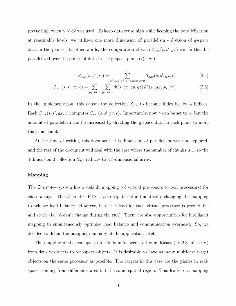
pretty high when γ ≤ 32 was used. To keep data reuse high while keeping the parallelization

at reasonable levels, we utilized one more dimension of parallelism - division of g-space

data in the planes. In other words, the computation of each Saux(s, s′, gx) can further be

parallelized over the points of data in the g-space plane G(s, gx).

Saux(s, s′, gx) =

C∑chunk of g−space c=0

Saux(s, s′, gx, c) (2.5)

Saux(s, s′, gx, c) =

∑gy in c

∑gz in c

Ψ(s, gx, gy, gz)Ψ∗(s′, gx, gy, gz) (2.6)

In the implementation, this causes the collection Sarr to become indexible by 4 indices.

Each Sarr(s, s′, gx, c) computes Saux(s, s

′, gx, c). Importantly, now γ can be set to ns but the

amount of parallelism can be increased by dividing the g-space data in each plane to more

than one chunk.

At the time of writing this document, this dimension of parallelism was not explored,

and the rest of the document will deal with the case where the number of chunks is 1, so the

4-dimensional collection Sarr reduces to a 3-dimensional array.

Mapping

The Charm++ system has a default mapping (of virtual processors to real processors) for

chare arrays. The Charm++ RTS is also capable of automatically changing the mapping

to achieve load balance. However, here, the load for each virtual processor is predictable

and static (i.e. doesn’t change during the run). There are also opportunities for intelligent

mapping to simultaneously optimize load balance and communication overhead. So, we

decided to define the mapping manually at the application level.

The mapping of the real-space objects is influenced by the multicast (fig 2.3, phase V)

from density objects to real-space objects. It is desirable to have as many multicast target

objects on the same processor as possible. The targets in this case are the planes in real-

space, coming from different states but the same spatial region. This leads to a mapping

10

Figure 2.7: CPAIMD-specific 3-D FFT implementation. 1-D FFTs in the “j” direction areperformed first in the planes. Pencils of data are communicated and two sets of 1-D FFTsare done in the “i-k” planes.

function

pe(R(s, p)) = P × p× ns + s

N × ns

(2.7)

where P is the total number of processors Note that we could also have tried to minimize

communication during the concurrent transposes with g-space planes (phases I and VI) by

assigning multiple real-space planes with same state index but different plane index together.

But the amount of communication involved in the transpose phase is smaller owing to the

sparseness of data in g-space.

The mapping of the g-space objects is slightly more complicated. In section 2.1.2, we

saw that Saux(sγ, s′

γ, p) requires communication with G(s . . . (s + γ − 1), p) and G(s′ . . . (s′ +

γ − 1), p). Hence this part of the computation would benefit if G(∗, p) were co-located, as is

the case with R. But using a mapping similar to that in equation 2.7 causes a problem of

load-imbalance: the distribution of load among planes in g-space follows the distribution of

points among discrete planar sections of a sphere. We describe how we dealt with this load

imbalance problem using different mapping schemes in section 4.

3D FFTs

Parallel 3-D FFTs have been dealt with by Cramer et. al., who use a transpose-based

method ([?]) and Haynes et. al., who use an alternative method with log(n) stages ([?]).

The multi-stage method has the advantage of lower per-message(α) cost but suffers from

higher per-byte(β) cost. We chose the transpose method to parallelize the FFTs since we

can control the number of messages exchanged through the libraries provided in Charm++,

and reduce the α cost. The 1-D and 2-D (serial) FFTs were performed by using FFTW

[?]. The transpose method requires the FFT to be performed in stages, first 2-D then 1-D

11

or vice-versa. We chose to do the 1-D FFTs and then 2-D FFTs as the orbitals have a

sparse distribution in their 3-D grid (fig 2.7(a)), in a sphere. Due to our choice, we could

control the number of FFT operations at a finer grainsize. Also, the transpose becomes less

communication intensive since the amount of non-zero data to be sent is reduced. This is

illustrated in figure 2.7

2.1.3 Performing the Multiple Parallel 3-D FFTs

The algorithm requires multiple (ns) 3-D FFTs to be performed. We perform these concur-

rently using Charm++. In each 3-D FFT, there is computation (FFT) part and a communi-

cation (transpose) part. On each processor, planes belonging to different states can reside,

and these are involved in independent 3-D FFTs. We are able to overlap the computation

of one 3-D FFT with the communication of several other 3-D FFTs, as seen in figure 2.8.

This is especially relevant on machines such as PSC Lemieux, where the nodes have a com-

munication co-processor that allows the main processor to continue computation while it

transfers data via remote DMA without processor intervention (as seen in [?]). This overlap

of computation and communication is made possible by Charm++, and its advantage over

the MPI-like synchronous model can not be overemphasized.

2.1.4 Non-local Computation

This computation (phase IX) involves computing the non-local matrix and using it to com-

pute forces. The non-local matrix “Z” is a ns ×N ×N ×N × natom matrix. The non-local

component of the forces requires both particle data (responsible for the natom part) and

g-space data (responsible for the N ×N ×N part).

The particle data is replicated on all processors using a Charm++ group. The g-space

data is decomposed using the G array and to access it, the objects performing the non-local

computation have to “borrow” it. This is achieved by creating a collection A that is bound

12

Figure 2.8: Overlapped Transposes in concurrent FFTs in Phase I, as seen in a timelineview. The x axis shows the time, and the y axis shows messages being processed on a subsetof the processors. Some messages (show with tails) create new messages, the communicationof which is overlapped with processing of other messages

Figure 2.9: Subroutines used in the particle computation

to the collection G. A has exactly one object for each object in G, and A(s, p) is always

present on the same processor as G(s, p).

To access the g-space data, A(s, p) performs a local computation to gain access to the

object G(s, p), and copies the g-space data. This allows it to compute a part of the Z

matrix (using the subroutine “computeZ(...)”, as seen in figure 2.9, corresponding to its

state index s, x-index p and all values of y-index, z-index and atom-index. Thus the Z

matrix is computed in a distributed manner.

Next the Z matrix is reduced over g-space. To do this, A(s, p) first reduces it over the y

and z dimensions, and objects A(s, ∗) collectively reduce it over the x dimension. The result

of the reduction is collected at A(s, 0) (again, refer figure 2.9). This is a essentially a vector

13

of size natom. One such vector is present at each A(s, 0), and hence the reduced Z matrix is

available in the form of reduced vectors.

Each reduced vector available at A(s, 0) is communicated back to the objects A(s, ∗),

where it is used to compute forces for the corresponding portion of g-space. These forces are

added with the forces computed using the electron density.

2.1.5 The Reduction to Form Probability Density in Real Space

(Phase II)

Once the 3-D FFTs are completed, thus making the states available in real-space, the elec-

tronic densities can be computed for each state. This is

ρ(x, y, z) =∑s

|Ψr(s, x, y, z)|2

Since the states are decomposed into planes, the computation of density can be parallelized

over each plane index (a total of N) in real-space. Thus there are multiple (N) reductions

in progress simultaneously. These involve relatively large amounts of data each, since the

real-space objects are densely populated (10,000 complex numbers, for our benchmark). Our

choice of mapping reduced the communication in this phase, since all the virtual processors

mapped to a physical processor tend to belong to the same plane number, allowing the

runtime system to add them up locally, before participating in processor-level reduction.

This was automatically achieved using Charm++’s built-in support for reductions among

subsets of virtual processors belonging to a single collection.

2.1.6 Rho Computations

Next, the real-space density can directly be used to compute the “Exchange-Correlation

energy”. This can be done as soon as the density is computed. This is seen in figure 2.10,

14

where each plane of the density calls the subroutine “rhoRSubroutine(...)” on its data and

gets the energies. After that, the fourier coefficients of the density can be used to compute

the “Hartree Energy”. For this, a copy of the densities is to be subjected to an 3-D inverse

FFT (phase IV), using a transpose. Now this data is subjected to “rhoGSubroutine(...)”, as

seen in 2.10.

The energies thus computed are summed (in parallel) and multicasts of degree ns are

performed from each of the N planes of real-space density, to states in real-space. After

performing 3-D IFFTs (phase VI) with a procedure essentially the reverse of that used for

the FFTs, forces are obtained in g-space and are used to modify the states.

Figure 2.10: The serial subroutines used in the ρ computations

2.1.7 Multicasts

The multicast operations (figure 2.3, phase V) are each-to-many type of communication

operations of degree ns each. They can be performed ([?]) in several ways.

1. Direct: each of the N planes of ρ sends ns messages to the corresponding real-space

planes. The problem with this approach is that it deluges the network card with

messages and causes inordinate delay in message delivery.

2. K-send: here each of N planes sends k messages, waits for a pre-specified amount of

time and then sends again. This allows the network congestion to reduce and improves

on the direct approach. But this method is problematic as the waiting period is difficult

to guage correctly and the problem of network contention is not addressed.

3. Ring: In the ring method, each of the N planes sends data to one of the ns states and

then the data is forwarded to some other state. The advantage is that at any stage

the number of messages in flight is P , and the network contention is reduced.

15

4. Multi-Ring The diameter of the ring determines the completion time of the multicast.

To reduce the completion time, we created multiple rings of smaller diameters that

performed the multicast in parallel. This approach works well with the mapping scheme

described for real-space planes, where several “next-hops” in the ring reside on the same

processor.

We tried each of the above methods of multicast and found that the ring method worked

best. Note that the all-pairs communication involved in orthonormalization (for which the

ring was not a good algorithm) is different from the communication in the multicast. In

all the multicast strategies mentioned above, the total volume of communication entering

a processor is identical. In contrast, the block-pairs approach reduces total volume of

communication for the all-pairs pattern.

16

Chapter 3

Parallel FFT Library

The ab-initio molecular dynamics program uses parallel transpose-based 3-D FFTs in several

phases (I, IV, VI). While the 3-D FFTs in phases I and VI are “sparse” (owing to the

sparseness of data distribution in g-space), the 3-D FFTs in phase phase IV are “dense”.

This is because the data distribution in real-space is dense. Such transpose-based FFTs are

a common occurrence in molecular dynamics applications ([?]), and we have developed a

Charm++-based parallel library for parallel transpose-based 3-D FFTs.

The basic abstraction provided by the library is that of a set of slabs (collection of

contiguous planes) belonging to 3-D space among which the 3-D FFT has to be done. As

seen in figure 3, (a), the library can be used to perform or 3-D FFTs involving different data

sets within the same set of objects. The user maintains the data within the slabs but all the

code for the transpose and partial FFTs in provided in the library.

To use the library, some components of the usage should be understood. First, for the

code to perform according to the user’s desire, a configuration object has to be created. This

(a)Mul-ti-pledata-sets

17

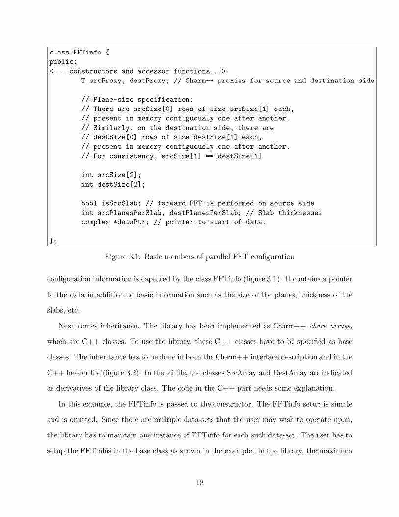
class FFTinfo {

public:

<... constructors and accessor functions...>

T srcProxy, destProxy; // Charm++ proxies for source and destination side

// Plane-size specification:

// There are srcSize[0] rows of size srcSize[1] each,

// present in memory contiguously one after another.

// Similarly, on the destination side, there are

// destSize[0] rows of size destSize[1] each,

// present in memory contiguously one after another.

// For consistency, srcSize[1] == destSize[1]

int srcSize[2];

int destSize[2];

bool isSrcSlab; // forward FFT is performed on source side

int srcPlanesPerSlab, destPlanesPerSlab; // Slab thicknesses

complex *dataPtr; // pointer to start of data.

};

Figure 3.1: Basic members of parallel FFT configuration

configuration information is captured by the class FFTinfo (figure 3.1). It contains a pointer

to the data in addition to basic information such as the size of the planes, thickness of the

slabs, etc.

Next comes inheritance. The library has been implemented as Charm++ chare arrays,

which are C++ classes. To use the library, these C++ classes have to be specified as base

classes. The inheritance has to be done in both the Charm++ interface description and in the

C++ header file (figure 3.2). In the .ci file, the classes SrcArray and DestArray are indicated

as derivatives of the library class. The code in the C++ part needs some explanation.

In this example, the FFTinfo is passed to the constructor. The FFTinfo setup is simple

and is omitted. Since there are multiple data-sets that the user may wish to operate upon,

the library has to maintain one instance of FFTinfo for each such data-set. The user has to

setup the FFTinfos in the base class as shown in the example. In the library, the maximum

18

number of data-sets allowed is a constant configurable at compile-time.

The easiest part is the actual usage - to perform a 3-D FFT from data-set 0 on the source

to data-set 1 on the destination side, the function doFFT(0,1) needs to be called. Once the

FFT and transpose is complete, the function “doneFFT(int id)” is called locally in the

destination slabs. Similarly, on completion of the inverse FFTs, the function “doneIFFT(int

id)” is called locally in the source slabs. The user should override the default definitions of

these functions as seen in the example.

19

In Charm++ .ci file:

mainmodule app {

extern module fftlib;

array [1D] SrcArray: NormalSlabArray {

entry SrcArray(NormalFFTinfo &conf);

};

array [1D] DestArray: NormalSlabArray {

entry DestArray(NormalFFTinfo &conf);

};

};

C++ inheritance:

class SrcArray: public NormalSlabArray {

public:

SrcArray(CkMigrateMessage *m) {}

SrcArray(NormalFFTinfo &info):NormalSlabArray() {

// normal setup

plane1 = new complex[info.srcSize[0] * info.srcSize[1] * info.srcPlanesPerSlab];

plane2 = new complex[info.srcSize[0] * info.srcSize[1] * info.srcPlanesPerSlab];

// Library-specific code

fftinfos[0] = new NormalFFTinfo(info);

fftinfos[0]->dataPtr = plane1;

fftinfos[1] = new NormalFFTinfo(info);

fftinfos[1]->dataPtr = plane2;

}

void doIt(int id) {doFFT(id, id);}

void doneIFFT(int id) {ckout << id << " Back" << endl;}

private:

complex *plane1, *plane2;

};

Figure 3.2: Example usage of the library: inheritance

20

Chapter 4

Performance and Optimizations

We ran our code on PSC Lemieux, a 750 node, 3000 processor cluster. Each node in Lemieux

is a Quad 1Ghz Alpha server connected by Quadrics Elan, a high speed interconnect with

4.5µs latency. The runs were performed with a g-space data set representing 32 water

molecules with a grid size of 100× 100× 100.

Figure 4.1: Number of non-local messages for different message sizes, on 1024 processors.There is total of 3.5 GB non-local communication per iteration.

Table 4.1 shows the scalability of the code. We achieved a peak floating point operations

rate of 121 GFlops on 1536 processors. Although this is a small fraction of the machine’s

capability, it is acceptable due to the communication intensive nature of this application.

Figure 4.1 shows the communication behavior of our code on 1024 processors. There is a

21

Nodes Processors Time(sec) GFLOPS Nodes Processors Time(sec) GFLOPS

8 16 13.260 4 43 129 2.2 2216 32 6.17 8 83 258 1.3 3732 64 3.110 15 171 513 0.680 7164 128 2.07 23 256 768 0.600 80128 256 1.18 41 512 1536 0.398 121256 512 0.650 74512 1024 0.480 100

Table 4.1: Execution times on PSC Lemieux, for 128 states. Using more processors per nodeaffects performance adversely as the bandwidth is a limited resource.

total of 3.5 GB of non-local communication, with the maximum data received per processor

being 5 MB. There are two modes of the distribution: the messages caused due to the 3-

D FFTs have sizes around 1KB, and the messages involved in the matrix computations in

orthonormalization have sizes around 20KB. These constitute the largest fraction of the non-

local communication. Notice that there are only one or two non-local messages per processor

that have a size greater than 100KB (multicast messages in phase V). This can be accredited

to the mapping scheme used for real-space planes (eqn 2.7) along with the multicast strategy

(multi-ring), which causes the most of the hops in the ring to be on-processor

To arrive at these results, we performed several optimizations, both algorithmic and

platform-specific. We explain the load-balance related optimizations in detail, with interme-

diate and final results.

4.0.8 Effect of Mapping on Load Balance

The effect of different mapping schemes is shown in figure 4.2, with “overviews” created by

the Projections performance tool, for 1024 processor runs. Each horizontal line corresponds

to one processor, with the x-axis showing progress in time (white color indicates a busy

processor). Using a map similar to equation 2.7 caused a load imbalance. The problem

is seen clearly in figure 4.2, (a), where the middle processors are significantly underloaded

compared with processor near 0 and 1023.

22

(a) Load imbalance due to phases I and IX(900ms)

(b) Improvement by using “wrapping”(590ms)

(c) Final result with load-vectors(480ms)

Figure 4.2: Solving the problem of load imbalance on 1024 processors

This was partially alleviated by using a modified version of 2.7:

pe(R(s, p)) = (4P × p× ns + s

N × ns

)%P (4.1)

This scheme assumes the presence of 4 times the actual number of processors, get the pro-

cessor number, and “wraps” it over the available number of processors, thus diversifying

the sizes of planes present on each processor. The result of this is seen in figure 4.2, (b).

23

Although better than before, it is clear (by looking at a few long lines in the overview figure)

that it does not achieve a good load balance, leaving a few highly overloaded processors.

We then explicitly took in to account the number of non-zeroes on each plane (alluded

to in section 2.1.2). We defined a “load-vector” L and a “cumulative” load-vector C of size

N and define the mapping in terms of them.

L[i] = number of non zeros in plane i over all states

C[i] =∑

j<=i

L[j]

pe(G(s, p)) =C[p− 1] + s

ns× L[p]

l(4.2)

where l =

∑pL[p]

P is the desired average load per processor

The best performance was obtained when we explicitly considered the load caused by

each g-space plane as in equation 4.2.

This mapping produced much better load balance, as seen in figure 4.2 However, it is

clear that transforming our knowledge of the number of non-zeroes in each plane into a

balanced mapping is difficult. We are therefore planning to use Charm++’s automatic load

balancers, modified to allow programmers to specify partial mappings (as we need for R, as

explained in Sec. 2.1.2). Our preliminary results in this directions have shown promise. E.g.

on 512 processors, the automatic balancer leads to a step time of 620 ms, as opposed to 650

ms with the above manual mapping.

24

Chapter 5

Conclusion

We have described the parallelization of the CP method using Charm++, and our efforts to

scale the benchmark to over 1500 processors, with a fixed problem size of 128 states. This is

unprecedented since all earlier efforts either find scaling beyond 128 processors difficult ([?],

or scale only when the problem size is proportional to the number of processors ([?]). Virtual-

ization and adaptive overlap of communication, automatically engendered by Charm++, are

clearly helpful for this application. Our results, both in absolute performance, and number

of processors used, mark a significant improvement.

The floating point performance achieved is a relatively small fraction of the peak ca-

pability of the machine. The large volume of data communicated non-locally (3.5 GB on

1024 processors) is primarily responsible for this and we have identified several avenues for

improvement.

The FFTs in g-space can be made more efficient by making assumptions about the nature

of data-distribution in g-space. For example, if we assume that along any one axis, there

are only two contiguous regions of non-zero data, the overhead when performing transposes

can be significantly reduced. Also, the data in g-space is conjugate symmetric and this can

be used to perform FFTs whilst “double-packing” the data. This will not only reduce the

amount of computation required, but also reduce the amount of communication involved in

the transposes.

The amount of communication involved in orthonormalization is very large in volume.

25

We intend to explore another dimension in the parallelization of the S matrix computation,

which will reduce the overall amount of data sent.

26

Appendix Software Implementation

Charm++ and our implementation of CPAIMD using it are freely available for download

at http://charm.cs.uiuc.edu. You can obtain the current code by following the links for

“Research” and “Ab initio molecular dynamics”.

Here is a list of the object collections used in the code and their corresponding Charm++

proxies.

• G(s, p): gSpacePlaneProxy.

This is a 2-D chare array, with the x-index being the state number and the y-index

being the plane number. Note that if there is more than one plane held in a sin-

gle array element, then the index is the smallest plane number among the available

plane numbers. The number of planes in each object is controlled by the variable con-

fig.gSpacePPC. Only the non-zero planes are inserted, and the axis of decomposition

is the x-axis.

• A(s, p): particlePlaneProxy.

This is a 2-D chare array, and is bound to the gSpacePlaneProxy, which implies that

the elements particlePlaneProxy(s, p) and gSpacePlaneProxy(s, p) are always present

on the same processor. This chare array is used for the particle/atom computation.

• R(s, p): realSpacePlaneProxy.

This also is a 2-D chare array, and its elements have the states in real-space. Again,

if there is more than one plane held in a single array element, then the index is the

27

smallest plane number among the available plane numbers. The axis of decomposition

is the y-axis, and the number of planes in each object is controlled by the variable

config.realSpacePPC.

• “ρ arrays”: rhoRealProxy and rhoGProxy.

The density in real-space is represented by a 1-D chare array, with proxy “rhoReal-

Proxy” and the density in fourier-space is represented by another 1-D chare array, with

proxy “rhoGProxy”. The structure of the rhoReal array reflects that of the realSpace-

Plane array. The axis of decompostion is the y-axis and the number of planes per

object is the same in the two arrays. The rhoG array has a different axis of decompo-

sition and the number of planes per object is controlled by config.rhoGPPC. The array

indices of both rhoReal and rhoG are continuous, i.e., even if there is more than one

plane per object, the array indices progress as 0, 1, 2, . . .

• Sarr(x, s1, s2, c): sCalculatorProxy

The parameter γ is controlled by the variable config.sGrainSize. The elements that are

inserted have s1 ¡= s2 and have x-coordinates corresponding to the non-zero planes.

Important groups and their uses:

• atomsGrpProxy: proxy for group used to replicate atom/particle information on all

processors.

• scProxy: proxy for group used for making QC-specific constants available on all pro-

cessors.

• sReducerProxy: proxy for group used for performing reductions over the Sarr elements.

28