Interoperability and computational framework for simulating open

channel hydraulics: application to sensitivity analysis and calibration of

Gironde Estuary model

Cedric Goeury, Yoann Audouin, and Fabrice Zaoui

Electricite de France (EDF), Research and Development Division, National Laboratory forHydraulics and Environment (LNHE), 6 Quai Watier, 78400 Chatou, France

July 5, 2021

Abstract

Water resource management is of crucial societal and economic importance, requiring a strong capacity foranticipating environmental change. Progress in physical process knowledge, numerical methods and computa-tional power, allows us to address hydro-environmental problems of growing complexity. Modeling of river andmarine flows is no exception. With the increase in IT resources, environmental modeling is evolving to meet thechallenges of complex real-world problems. This paper presents a new distributed Application ProgrammingInterface (API) of the open source telemac-mascaret system to run hydro-environmental simulations withthe help of the interoperability concept. Use of the API encourages and facilitates the combination of worldwidereference environmental libraries with the hydro-informatic system. Consequently, the objective of the paper isto promote the interoperability concept for studies dealing with such issues as uncertainty propagation, globalsensitivity analysis, optimization, multi-physics or multi-dimensional coupling. To illustrate the capability ofthe API, an operational problem for improving the navigation capacity of the Gironde Estuary is presented.The API potential is demonstrated in a re-calibration context. The API is used for a multivariate sensitivityanalysis to quickly reveal the most influential parameters which can then be optimally calibrated with the helpof a data assimilation technique.

Software availability

The Application Programing Interface (API) framework described in this article (Fortran APIs and its Pythonwrapper) is available for download in telemac-mascaret system (www.opentelemac.org). telemac-masca-ret is an integrated suite of solvers for use in the field of free-surface flow, available under the GNU General PublicLicense version 3.

1 Introduction

Water availability and quality are vital to human health. Increasing global scarcity makes anticipating the evolutionof this limited natural resource even more essential. This ability relies on the understanding and prediction ofhydrodynamic flows. Hydraulic simulation codes (such as hec-ras [22], mohid [48], delft-3d [20], telemac-ma-scaret [34]) have been developed for many years and applied to a wide range of hydro-environmental cases, suchas prevention of flood risks [71], development of management plans [63] or design schemes for flood alleviation [55].

Hydro-environmental modeling of river and marine flows is increasingly complex and requires a better knowledgeof physical and biochemical processes, advanced numerical methods and high-performance computing resources.For many applications, engineers have to deal with complex “modeling systems” for the representation of subparts ofa physical system [8, 32]. Increasing a numerical model conceptual complexity in terms of how many aspects of theunderlying system are included in it has the potential to improve the accuracy of the results in term of descriptiveand predictive capacities. However, adding each new aspect to the model can induce an increase of the error broughtabout by the uncertainty in the description of the features accumulates and increases the overall uncertainty inthe output [14, 44] . This trade-off between “model completeness” and “propagation error” [66] is known as the

1

arX

iv:2

012.

0911

2v2

[cs

.CE

] 2

Jul

202

1

conjecture of O’Neill [56]. In maritime or fluvial cases, numerical modeling tools allow replicating the past aswell as predicting the future with an uncertainty range that is strongly linked to the approximate description ofhydraulic parameters [59], meteorological data [4] and geographical data [1]. In spite of the significant improvementin computational resources and the accuracy of numerical models, the turbulent nature of fluid mechanics equationslimits the performance of hydraulic models. The need for realistic hydrodynamic flow simulation is beyond theabilities of deterministic forecast. As a consequence, model uncertainties have to be quantified. Recent advances insimulation and optimization of environmental systems have relied on increasingly detailed models, running manyscenarios, in order to quantify these uncertainties [33, 71].

According to Solomatine and Ostfeld [68], significant advances in the means of observing continental waters,especially through orbital equipment (SWOT satellite mission [51]; Sentinel satellite missions (Copernicus program)[46]), allows use of various types of data, with their associated analysis, for water resources management [40]. Thus,environmental modeling is increasingly complemented by data-driven models [37]. Moreover, by taking into accountadvances in information processing and data management, it becomes possible to reduce uncertainties and betterunderstand the modeling process. Data-driven modeling is a paradigm shift for addressing many problems inscience and engineering [49].

To summarize, with the increase in computer resources, environmental modeling is evolving with the need tosolve increasingly complex real-world problems involving the environment and its relationship to human systemsand activities. If it is to break down research silos, and bring scientists, stakeholders and decision-makers together tosolve social [17], economic [31] and environmental problems, an environmental modeling system should support ITtasks, such as aggregation of model components into functional units, component interaction and communication,parallel computing and cross-language interoperability [19, 43]. These technical requirements are closely relatedto interoperability aspects, namely the capacity of the software to run and share information with other codes.Environmental system development requires both scientific understanding of the phenomena involved and softwaredevelopment proficiency.

This paper presents a new Application Programming Interface (API) of the open source and interoperable te-lemac-mascaret system (http://svn.opentelemac.org/svn/opentelemac/) to solve environmental problems[28, 41]. Since 2017, the telemac-mascaret system has included in its distribution a generic API that allowsit to expand its range of applications [5]. With this newly implemented feature, the telemac-mascaret systemcan be easily coupled or integrated into higher-level platforms to model, study or simulate complex problems [27].

To our knowledge, APIs for an environmental modeling system (with hydraulic (mascaret 1D, telemac-2d,telemac-3d), water quality (tracer, waqtel), sediment transport (courlis, gaia), and wave hydrodynamics(tomawac and artemis)) are not yet widespread in the environmental community and are an original innovation.The present work uses as an example France’s Gironde Estuary to demonstrate the operational applicability andoutcomes of APIs. The port of Bordeaux in the Gironde Estuary faces many development challenges [38]. Tosatisfy demand for larger ships, while ensuring navigational safety, the evolution of water depth over time in theestuary needs to be predicted with a high degree of accuracy. To address this issue, the numerical results mustbe consistent with past observational data. Among other things, this process relies on calibration to determine“empirical adequacy” [57]. In particular, the calibration aims at simulating a series of reference events by adjustingsome uncertain physically-based parameters until the comparison is as accurate as possible [21]. The objectiveof this work is to implement an efficient calibration algorithm, capable of processing measurement optimally, inorder to estimate the partially known or missing parameters [53]. Often performed, calibrating a hydrodynamicmodel is nevertheless a difficult task owing to the complexity of the flows and their interaction with the shoreline,the bathymetry, islands, etc. It is essential to understand, in depth, the relationship between the calibration ofmodeling parameters and the simulated state variables which are compared to the observations. In this context,a multivariate sensitivity analysis [23, 42] succeeded in identifying the most influential input parameters on themodel results. Sensitivity analysis is associated to define the parameters to be calibrated using a physically baseddata-driven technique [12].

This paper is organized as follows. Section 2 includes a description of the main concepts of the telemac-ma-scaret system API. Section 3 presents the architecture of implemented APIs. Section 4 describes the applicationcase. Section 5 deals with the calibration problem. Section 6 is the discussion and Section 7 is the conclusion.

2 Method

The telemac-mascaret hydro-informatic system, created in 1987, is an open source (www.opentelemac.org)integrated suite of solvers for use in the field of free-surface flows [34]. As displayed on Figure 1, it can carryout simulations of flows (mascaret, telemac-2d and telemac-3d, gray circle), sediment transports (courlis

2

and gaia, orange circle), waves (artemis and tomawac, green circle) and water quality (tracer and waq-tel, purple circle). Historically, from the original software solving physics equations (Saint-Venant: mascaretand telemac-2d, Navier-Stokes: telemac-3d, elliptic mild slope equation: artemis, simplified equation for thespectro-angular density of wave action: tomawac, Exner: courlis and gaia, water quality processes: tracerand waqtel), the system has gradually evolved to the notion of hydro-informatics with a set of solvers dealing withlarge heterogeneous data and solving complex dependent problems (overlapping physical components in Figure 1).The various simulation components use high-end algorithms based on the finite element or finite volume method.The ability to study global, regional, or local scale problems by using the same system, makes the telemac-ma-scaret a useful tool for assessing the environmental state in the sea, estuaries, coastline and rivers.

Hydraulic:mascaret (1D)telemac-2d (2D)telemac-3d (3D)

Water quality:tracer (1D)waqtel (2D & 3D)

Waves:artemis (2D)tomawac (2D & 3D)

Sediment:courlis (1D)gaia (2D & 3D)

Figure 1: telemac-mascaret hydro-informatic system

According to Laniak et al. [43], Integrated Environmental Modeling (IEM) highlights the importance of softwaredevelopment and sharing in their role as pluggable components of a larger ecosystem. The work presented hereis part of this trend. It shows the implementation procedure for the component-based solver interoperability ofthe telemac-mascaret system. The API architecture, described in this paper, is directly applicable for anysoftware regardless of its language since it is an easy task to build a wrapper in other programming language aspresented in the following for Fortran and Python. The main difficult part is to split the software main program.When a solver is an interoperable component, it can be part of an assembly of elements in permanent interactionthat work in a coordinated way. To be considered as an elementary reusable component, a computation modelmust:

• possess APIs, which can be viewed as new functionalities or entry points in the computational model toprovide new services on demand;

• have a resolution algorithm comprising three main functionalities: problem initialization, simulation andfinalization of the computation;

• allow instantiation of several clearly separated and identifiable problems;

• be usable in dynamic library form.

In the following, the four points listed above are addressed.

3

2.1 Design

A computer programming model like the object-oriented programming (OOP) aims to organize the software designaround data grouped into objects with attributes and methods. This help the developper to focus on the data ratherthan the logic required to manipulate them. Most of the OOP concepts (encapsulation, interfaces, polymorphism,modularity, instantiation, . . . ) are derived from software engineering patterns but relate to the real world. Asshown in Figure 2, the first concept used here is Encapsulation with a classic Design Pattern “Facade” [24]. Sincethe telemac-mascaret system is written in Fortran 77 and 90, the design pattern has been adapted to this nonobject-oriented language as OOP is well-suited for the design of large and complex programs.

User calls

Facade

module 1

module 2 · · ·module n

Fortran sources of component-based solver

Figure 2: Design Pattern “Facade”

The main benefits of this approach are that it is easier to use and understand, limits the library user depen-dencies, includes integrity constraints and validation rules and avoids some unnecessary calculations [41].

Internal data has been accessed in order to expand the capabilities of the API. It is possible to examine all theinformation embedded in the calculation code and modify its structure (specifically the values, some metadata andproperties) at runtime. Pointers were used to access the simulation data. As Fortran lacks the pointer definitionof other high-level languages such as C or C++, a combination of the POINTER and TARGET Fortran keywords withadequate updates were employed. For instance, a manually update must be done if a pointer on an ALLOCATABLE

variable is set before the dynamic allocation since the pointer is no longer valid. This ensures the correct state ofthe controlled variable. A component-based approach was adopted by having the same structure as all of the te-lemac-mascaret physical-dedicated solver, to allow them to be viewed as linkable. The execution of a simulationwas partitioned to allow modification of a given parameter at runtime (for example, each time step). The flexibilitythat comes with interoperability allows deployment of the telemac-mascaret system in specific industrialapplications and distribution of telemac-mascaret solvers as a part of complex modeling system (Applications,blue part in Figure 3). As mentioned by Gil et al. [26], geosciences “will lead to a new generation of knowledge-richintelligent systems that contain rich-knowledge and context in addition to data, enabling fundamentally new formsof reasoning, autonomy, learning, and interaction”. As presented in Figure 3, the telemac-mascaret physical-dedicated components can be easily connected together to build multi-physics or multi-dimensional interactions[32] (Coupling, orange part), inserted in optimization or uncertainty quantification processes (Studies, yellow part,see Section 5), wrapped in advanced technology such as cloud-based solutions or embedded systems with datamanagement (OpenMI [29] or Pynsim [39], Cloud services, green part) and integrated in platforms (Salome [64] orPalm [9] for example, Numeric computing environment, pink part).

4

TELEMAC

API

Numeric

Computing

Environmen

ts

Applications

Coupling

Cloud

Services

Studies

Robustness

Modelling

C/C++/Fortran

Salome

Julia

R

Python

Notebook

Data processing

SaaS

Cloud Computing

Geosciences E

ducation

Industry

Multi-Physics

Multi-Dimensional

Multi-Fidelity

Training

Documentation

Matlab

Discretization

Representation

Optimization

Hydrology

Hydraulics

Water Qua

lity

Sedimen

tology

Surrogate

Direct

Parametric

Uncertainty

Quantification

Sensitivity

Analysis

Calibration

Shape

Data

Assimilation

Regulation

Convergence

River &

Coastal Flow

Reservoir

Tsunami

Morphodynamics

Pollution

Ice

Temperature

Figure 3: Ecosystem of the telemac-mascaret API

2.2 Technology

To maintain efficient execution, a native code compiler (for example, GNU Compiler Collection, licensed under GNUGPL) running on most systems and hardware architectures, and supporting Fortran, is used and recommended.Moreover, the calculation code of the telemac-mascaret system numerically solves a model based on a systemof partial differential equations (PDE). The computational solution relies on an implicit time scheme, removingstability constraints on the time frame, but leading to a linear-system solution of considerable size. The resultingincreased complexity of the model structures poses strong limitations in terms of practical implementation andcomputational requirements. Consequently, High-Performance Computing (HPC) is necessary to tackle realisticapplications. The solution deployed in the hydro-informatic system is to decompose the domain of computation.This idea of domain decomposition is to assign to each processor one part of the global domain over which it solvesthe fluid mechanics problem. The results of the other processors help in defining artificial boundary conditionsarising from the partition. The assignments given to each processor are the same, but the data differ. Therefore,the telemac-mascaret system requires the use of an MPI library for communication between processors [16].

It is possible to use MPI technology for the instantiation of several clearly separated and identifiable problems.This is because MPI is adapted for distributed memory systems. This method has been followed for the learningstep of sensitivity analysis presented in Subsection 5.1.

5

3 Architecture of API

The architecture is generic for all telemac-mascaret system components (Figure 1). For the sake of clarity,only an API example with the telemac-2d component is shown in the following sections.

3.1 Fortran structure

API’s main goal is to control the simulation while running a case. For example, it must allow the user to suspend thesimulation at any time step, retrieve some variable values, and possibly change them before resuming the calculation.To make this possible, a Fortran structure called “instance” is used in the API. The instance structure gives directaccess to the physical memory of variables, and therefore allows control of the variable. Furthermore, based ondecomposition of the main telemac-mascaret system subroutines in three main functionalities (initialization,simulation of one time step and finalization), it is possible to run a hydraulic case for an indefinite sequence of timesteps.

Figure 4 describes an example of API workflow where X are input parameters and O(t) is information extractedat given times. For instance, in the framework of the Gironde Estuary application case, X represents parametersto be estimated / calibrated (friction coefficients and tidal boundary condition parameters) and O(t) is the freesurface elevation every minute at the measurement stations (see Section 4).

Input parameter vector X = (X1, ..., Xp)′

Configuration setup (initializeinstance ID and listing output)

CALL RUN_SET_CONFIG_T2D

Set study physical andnumerical parameter

CALL RUN_READ_CASE_T2D

Set the initial condi-tion of computation (t0)

CALL RUN_ALLOCATION

CALL RUN_INIT

Change the parametervalues according to X

CALL SET_DOUBLE

Run one time stepof the solver (ti)

CALL RUN_TIMESTEP_T2D

Get the output de-sired values O(ti)

CALL GET_DOUBLE

i <= n

Conclude solver computation(deallocation, and so on)

CALL RUN_FINALIZE_T2D

O(t) = M (X, t)

no

yes

Figure 4: Diagram of study workflow (Function M (X, t) in Figure 7) and corresponding Fortran API calls

For each action defined above, the identity number of the instance is used as an input argument allowing

6

all computation variables to be linked with the corresponding instance pointers. These actions must be done inchronological sequence in order to ensure proper execution of the computation in the API main program. In Fortranand for the shallow water code telemac-2d, it will begin with the call of an initialization subroutine:

CALL RUN_SET_CONFIG_T2D(ID , LU , LNG , COMM , IERR)

where all parameters are scalars of type integer and ID is an output value giving the instantiation number. Theinput parameter LU is used to redirect the standard output, LNG has only two possible values for the choice of theenglish or french language, and COMM is the MPI communicator for the distributed-memory parallelism. The outputIERR has to be considered with care as a non-null value stands for the occurrence of errors. A systematic test onthis return value is recommended, for instance one may want to stop the program accordingly:

IF (IERR.NE.0) EXIT IERR

After the initialization phase, the model has to be read from files with the following instruction:

CALL RUN_READ_CASE_T2D(ID , CAS_FILE , DICO_FILE , INIT , IERR)

The name of the steering file is given with CAS_FILE as a character string, it stores several input data of themodel with key-value pairs. Each possible key is set with a dictionary file whose name is a character string holdby DICO_FILE. A true value for the logical input INIT will initialize a common computational kernel of all themodules. After this step, a dynamic allocation of arrays in memory is necessary followed by a state initializationof the physics:

CALL RUN_ALLOCATION_T2D(ID , IERR)

CALL RUN_INIT_T2D(ID , IERR)

All accessible parameters are listed in predefined keyword lists (see Appendix A for telemac-2d). For example,the number of time steps in the simulation is named MODEL.NTIMESTEPS and its value is obtained and stored in thevariable NBSTEPS with the following call:

CALL GET_INTEGER(ID , "T2D", "MODEL.NTIMESTEPS", NBSTEPS , 0, 0, 0, IERR)

Input parameter can be defined here using the following call:

CALL SET_DOUBLE(ID , "T2D", "MODEL.SEALEVEL", SEALEVEL , 0, 0, 0, IERR)

where the sea level value in the computation (accessed through the keyword MODEL.SEALEVEL) is set to the valueof the variable SEALEVEL.

Now the simulation can be done with a loop on the number of time steps while storing all the results of anevolution of the water depth:

DO I = 1, NBSTEPS

CALL RUN_TIMESTEP_T2D(ID , IERR)

CALL GET_DOUBLE(ID , "T2D", "MODEL.WATERDEPTH", WATERDEPTH(I), 42, 0, 0, IERR)

ENDDO

WATERDEPTH is a one-dimensional array of size NBSTEPS. It is used here to store the water depth values at nodenumber 42 of the telemac-2d triangular mesh. Finally, the Fortran program can end with the instance deletionthus freeing the memory used:

CALL RUN_FINALIZE_T2D(ID , IERR)

Additional functions are available to handle parallelism (see Subsection 2.2 for more details on parallelism in thetelemac-mascaret system). The data structure in the current version (official version 8.2) does not yet allow formultiple instantiations, as all the instances point to the same memory area. This constitutes a future developmentto improve API capacity. However, instantiation associated with the processor communication function overcomesthis limitation by ensuring the possibility of several clearly separated and identifiable problems.

3.2 Python wrapping

The use of API is not limited to Fortran programing but can also be used by a scripting language. To this end,a Python wrapper is also available. It is relatively easy to use the Fortran API routines directly in Python usingthe f2py tool of the Python Scipy library [60]. This tool will make it possible to compile Fortran code for use inPython. The only limitations are on the type of arguments of the functions to wrap. Python is a portable, dynamic,

7

extensible, free language, which allows (without requiring) a modular approach and object-oriented programming[73]. In addition to the benefits of this programming language, Python offers a large number of interoperablelibraries for scientific computing, image processing, data processing, machine learning and deep learning. The linkbetween various interoperable libraries with telemac-mascaret system APIs allows the creation of an ever-moreefficient calculation chain capable of responding finely to various complex problems such as the application casepresented in this article (see Section 4). Moreover, the Python scripting language makes it possible to implementa wrapper in order to provide user-friendly functioning of the Fortran API. Thus, a Python overlay was developedto encapsulate and simplify the different API calls.

For instance, a Python “get” function can encapsulate all API Fortran type-dedicated function get type (wheretype can be replaced by Double, Integer, Boolean and String). File management is also made easier with Python(copy, move, . . . , and reducing the number of arguments). This Python wrapping of telemac-mascaret systemAPI constitutes a package called TelApy distributed in the official version of the hydro-informatic system (Figure5).

TelApy module

Fortran API

Main function of APImodule api interface

TELEMAC-2D solver

instantiation moduleapi instance t2d

Variable controlapi handle var t2d

Computation controlapi run t2d

TELEMAC-3D solver

instantiation moduleapi instance t3d

Variable controlapi handle var t3d

Computation controlapi run t3d

solver ...

Python wrapper

Class api module

Class t2d

Specific function forTELEMAC-2D

Class t3d

Specific function forTELEMAC-3D

Class ...

Specific function for...

Figure 5: Overview of TelApy module

The TelApy package is provided with a tutorial for people who want to run the telemac-mascaret sy-stem physical components in an interactive mode with the help of the Python scripting language. The scriptcorresponding to the application case of Section 4 is presented in Appendix B.

3.3 Summary

A single coherent Fortran structure has been deployed in telemac-mascaret in order to ensure interoperabilityof the system for each of its solvers. This is based on three main functionalities: instantiation, variable valuesand computation control. Firstly, instantiation associated with the processor communication function ensuresthe possibility of a simultaneous existence of several clearly separated and identifiable problems. Secondly, basedon variable and computation control, memory access is permitted during simulation, allowing new services tobe provided on demand. Finally, the technology allows dynamic compilation of each physical-based componentmodel. All of these features enable the telemac-mascaret system to operate with other existing or futurecodes without restricting access or implementation. It therefore becomes natural to drive these APIs using Pythonscripting language. As mentioned by Knox et al. [39], this scripting language offers numerical and scientific librariesand is already a recognized tool in environmental resource modeling.

Finally, the Python wrapping allows use of the telemac-mascaret system for a wide range of studies, suchas optimization, coupling and uncertainty quantification.

The Application Programing Interface (API) framework described in this work (Fortran APIs and its Pythonwrapper) is available for download and distributed in telemac-mascaret system (www.opentelemac.org).

4 Gironde Estuary application case

The hydrodynamic model telemac-2d was used to solve the shallow water equations (see Section 4.2) in the realcase of the Gironde Estuary in southwestern France (Figure 6). This important large-scale estuary involves many

8

economic and environmental considerations. Several hydrodynamic and morphodynamic telemac-2d studies ofthe estuary have been carried out for the last decade [35, 74]. In these studies, the importance of the calibrationphase was systematically emphasized to achieve operational performance.

Figure 6: Gironde Estuary. Location of observation stations (•), bathymetry, friction zones (Ks denotes Stricklercoefficient) and mesh size [76]

Model calibration aims at simulating a series of reference events by adjusting some uncertain physically basedparameters in order to minimize deviation between measured and computed values of variables of interest. Thisprocess of parameter estimation, a subset of the so-called inverse problems, consists in evaluating the underlyinginput data of a problem from its solution. For free-surface flow hydraulics, parameters that are often unknown ordifficult to assess include initial state, bathymetry, bed friction and model boundary conditions. In this work, thebathymetry and initial state are considered as known. In fact, a spin-up of 12 hours was used to generate realisticinitial condition. Bathymetry uncertainty was not considered in this study and could constitute an approximationin particular on current speed [13]. A primary challenge of integrating bathymetry in the calibration process is thespatial structure characterization of its uncertainty in relation to channel morphology [45]. This was not studiedhere and will be the topic of a future study. Consequently, both bed roughness and model boundary conditions areconsidered in the calibration process. As mentioned by Williams and Esteves [75], the hydrodynamic bed friction isa primary calibration variable for all coastal and estuarine models. It is also essential for modeling other processesaccurately such as sediment transport and wave attenuation. Concerning the model boundary conditions, onlyoffshore boundary condition is considered in the calibration process as it is derived from a coarser-scale model andupstream boundary conditions is coming from measurement. The transfer of information between a large scalemodel and the boundaries of a more local model generally requires empirical adequacy: sea level could need tobe corrected to account for seasonal variability (effect of thermal expansion, salinity variations, air pressure, etc.)in addition to long-term sea level rise resulting from climate change and differences in tidal amplitude could beattributable to meteorological effects (storm and surge (atmospheric and wave setup)) [36]. Although this paperfocuses on friction and tidal parameters, all telemac-2d variables can be changed by the API, as presented inTable A.1.

4.1 Numerical configuration and available data

The Gironde is a navigable estuary in southwest France formed by the confluence of the Garonne and Dordognerivers just downstream of the center of Bordeaux. The Gironde Estuary is the largest estuary in western Europe.The hydraulic model covers approximately 195 km between the fluvial upstream and the maritime downstream

9

boundary conditions, for an area of around 635 km2. The finite element mesh is composed of 173, 781 nodes (Figure6). The mesh size varies from 40 m within the area of interest, the navigation channel, to 750 m offshore (westernand northern sectors of the model). As shown in Figure 6, six friction areas are considered in the hydraulic model.

The boundary condition along the marine border of the model was set using depth-averaged velocities andwater levels from the Legos numerical model TUGO dataset (46 harmonic constants). Surge data, describing thedifference between the tidal signal and the observed water level, are taken into account using a data file generatedfrom the Hycom2D model of the SHOM [15]. Surface wind data are also considered to simulate the flow underwindy conditions. Time-evolution flow discharge hydrographs are imposed upstream of the Gironde Estuary modelon the Garonne and Dordogne rivers. The ability of the numerical model to reproduce complex physical processessuch as sediment transport is presented in [58].

The free surface flow was continuously measured (every minute) at the Verdon, Richard, Lamena, Pauillac, FortMedoc, Ambes, The Marquis, Bassens and Bordeaux locations (Figure 6). For this study, observation results areused over a 36 hour period from August 12 to 14, 2015.

4.2 Hydrodynamic model

The telemac-2d code solves the 2D depth-averaged free surface flow equations, also known as shallow waterequations (Eqs. 1-3).

∂h

∂t+

∂

∂x(hu) +

∂

∂y(hv) =0 (1)

∂hu

∂t+

∂

∂x(huu) +

∂

∂y(huv) =− gh∂Zs

∂x+ hFx +∇ · (hνe∇ (u)) (2)

∂hv

∂t+

∂

∂x(huv) +

∂

∂y(hvv) =− gh∂Zs

∂y+ hFy +∇ · (hνe∇ (v)) (3)

where x and y are the horizontal Cartesian coordinates, t the time, u and v the components of the depth-averaged velocity, h the water depth, νe an effective diffusion representing depth-averaged turbulent viscosity νtand dispersion, Zs the free surface elevation, g the gravitational acceleration, Fx and Fy refer to the friction force(see Section 4.2.1).

telemac-2d solves the previous equation system using the finite element method on a triangular elementmesh. The main results at each node of the computational mesh are the water depth and the depth-averagedvelocity components. telemac-2d can take into account propagation of long waves, including non-linear effects,bed friction, effect of the Coriolis force, effects of meteorological phenomena (e.g., atmospheric pressure, rain orevaporation, and wind), turbulence, supercritical and subcritical flows, influence of horizontal temperature andsalinity gradients on density and dry area in the computational domain, amongst other processes [34].

4.2.1 Friction coefficient

The friction term in the momentum part of the shallow water equations is treated in a semi-implicit form withintelemac-2d. The two components of friction force are given in Eq. 4.

Fx = − u2hCf

√u2 + v2

Fy = − v2hCf

√u2 + v2

(4)

where Cf is a dimensionless friction coefficient.The roughness coefficient often takes into account friction caused by walls on the fluid or other phenomena such

as turbulence. Empirical or semi-empirical formulas are used for calculating Cf [52]. In the present work, Cf isgiven by the widely used Strickler formulas (Eq. 5). The Strickler coefficient (m1/3s−1) is a calibration parameterof the modeling system, to be adjusted according to field data (e.g., usual measured water levels).

Cf =2g

h1/3K2s

(5)

Generally, the friction coefficient is contained in an interval bounded by physical values, as it results fromdifferent contributions (e.g., skin friction, bed form dissipation, etc.). In this study, the Strickler bounds are takenas large as possible. In fact, the lower bound of the Strickler coefficient is set to 5 according to U.S.F.H.A [72](rough bed surface) and the upper one is set to 115 (extreme smooth bed surface).

10

In the present API context, the friction coefficient is called MODEL.CHESTR and in the study corresponds to theStrickler coefficient Ksi (where i denotes the considered friction area).

4.2.2 Tidal amplification parameter

Tidal characteristics are imposed using a database of harmonic constituents to force the open boundary conditions.For each harmonic constituent, the water depth h and components of velocity u and v are calculated, at point Pand time t by Eq. 6.

f (P, t) =∑i fi (P, t)

fi (P, t) = fi (t)Afi (P ) cos[2πtTi− ϕfi (P ) + ϕ0

i + li (t)]

(6)

where f is either the water depth h or one of the components of velocity u or v, i refers to the consideredconstituent, Ti is the period of the constituent, Afi is the amplitude of water depth or one of the horizontalcomponents of velocity, ϕfi is the phase, fi (t) and li (t) are the nodal factors and ϕ0

i is the phase at the originaltime of the simulation. The water level and velocities of each constituent are then submitted to obtain the waterdepths and velocities for the open boundary conditions (Eq. 7). h = α

∑i hi − Zb + Zref − γ

u = β∑i ui

v = β∑i vi

(7)

where Zb is the bottom elevation and Zref the mean reference level. In Eq. 7, the tidal amplitude multipliercoefficients of tidal range and velocity, respectively α and β, at boundary locations and the sea level correction γare assumed to be the tidal calibration parameters [61].

The sea level correction parameter is assumed, following expert opinion, to be contained in an interval of plus orminus a meter. The interval of the weighting coefficients of tidal range and velocity is set to [0.8, 1.2] correspondingto a 20% margin of the initial value.

In the API framework, the sea level correction variable γ is designated as MODEL.SEALEVEL, and the weightingcoefficients of tidal range α and velocity β are denoted MODEL.TIDALRANGE and MODEL.VELOCITYRANGE, respectively.

4.3 Summary of parameter range variation

All the model input parameters and their associated probability distribution are summarized in Table 1.

Variable name Nature Variation interval Probability distribution

Fiction coefficient per area (m1/3s−1) Real scalar [5., 115.] UniformSea level correction parameter (m) Real scalar [−1., 1.] UniformTidal range coefficient (−) Real scalar [0.8, 1.2] UniformVelocity range coefficient (−) Real scalar [0.8, 1.2] Uniform

Table 1: Input parameters and associated probabilistic model for the Gironde Estuary application

5 Calibration problem

The inverse problem of calibration can be understood as the computation of the posterior distribution π (X|Y)(“Model Calibration Algorithm step”, Figure 7, as presented in appendix C), where model parameters constitute thep-components of the parameter control vector X = (X1, ..., Xp)

′ ∈ Rp composed of independent variables definedon some probability space (Ω, A,P) (with Ω as a sample space, A the σ-algebra of events and P the probabilitymeasure), Y ∈ Rm is the observation vector, also defined on a probability space, around the unknown parametervector X and Rm is the observation space defined by Eq. 8.

Y = G (X) + εm (8)

where G : Rp −→ Rm is a vector-valued function of vector X and εm ∈ Rm is an observable measurement noisesuch as E (εm) = 0 and R = cov(εm) = E (εmε

′m) ∈ Rm×m and identified as a multivariate normal distribution,

εm ∼ N (0,R). As a reminder, in the Gironde Estuary application case, the parameter control vector X is composed

11

of the friction and tidal parameters and the observation parameter Y is composed of water levels measured everyminute at an observation station. Note that the operator G enabling the passage from the parameter space (wherevector X lives) to the observation space (where vector Y lives) represents a call to the API study workflow definedin Figure 4. As telemac-2d is a discrete time dynamic model, the output O is composed of scalar output (waterelevation at observation stations interpolated from telemac-2d computational nodes given at t ∈ T = [1, .., T ]).

MODEL.CHESTR (6 areas)MODEL.SEALEVEL

MODEL.TIDALRANGE

MODEL.VELOCITYRANGE

Model telemac-2d M (X, t)Prior Knowledge π (X)

X

π (X)

Model Calibration Algorithm

Direct Model Evaluation

Result π (O)

O

π (O)

Observations (Y)

Posterior Knowledge π (X|Y)

X

π (X|Y)

Figure 7: Model calibration under uncertainty using observations framework

Finally, the maximum a posteriori is equivalent to the optimal search for the control vector minimizing theobjective function J (X) = 1

2 [X−X0]B−1 [X−X0]′+ 1

2 [Y −G (X)]R−1 [Y −G (X)]′

(where B is the prior co-variance matrix). This is known as the traditional variational data assimilation cost function, called 3D-VAR[12].

Mathematical methods can be used to solve optimization problems. The former can vary significantly accordingto the form of the cost function (convex, quadratic, nonlinear, etc.), its regularity, and the dimension of thespace. Many deterministic optimization methods are known as gradient descent methods, among which is theBroyden-Fletcher-Goldfarb-Shanno (BFGS) quasi-Newton method used in this work [50]. Using this constrainedoptimization method makes it possible to impose boundaries during the research process of the model parameters,guaranteeing their physical values. Because the inverse problem is often ill-posed and unstable with available datacorresponding to more than one solution, small changes in model results can lead to very different estimates for theinput (calibration) parameters. These problems are related to the issue of “parameter identifiability” [54]. Still, thechosen optimization method involves computing the adjoint of the observation operator G (or the partial derivativesof the operator with respect to its input parameters). In this work, the partial derivatives are approximated usinga classical finite difference method. This is a simple solution, numerically sensitive and computationally time-consuming, but the observation operator can be written to make use of parallel computing, thus providing a fastautomatic calibration algorithm relevant to real-world applications.

As the inverse problem is defined, a relevant question is what are the effects of the modeling calibrationparameters X on the simulated state variables O (t) = M (X, t) which are compared to the observations? Thisquestion can be addressed by multivariate sensitivity analysis.

5.1 Multivariate Sensitivity Analysis

The sensivity analysis aims at quantifying the relative importance of each input model parameter. The variance-based methods aim at decomposing the variance of the output to quantify the participation of variables consideredas independent. Conventional approaches to Global Sensitivity Analysis (GSA) compute sensitivity indices calledSobol’ indices and assume that the output variable is scalar. The definition of Sobol’ indices is a result of the ANOVA(ANalysis Of VAriance) variance decomposition [65, 67]. However, as reported by many authors [11, 25, 42], whenthis approach is applied to each variable of a functional output, it leads to a high degree of redundancy because of the

12

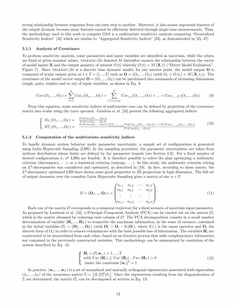
strong relationship between responses from one time step to another. Moreover, it also misses important features ofthe output dynamic because many features cannot be efficiently detected through single-time measurements. Thus,the methodology used in this work to compute GSA is a multivariate sensitivity analysis computing “GeneralizedSensitivity Indices” [42] which are similar to “Aggregated Sensitivity Indices” [23], as demonstrated in [25, 47].

5.1.1 Analysis of Covariance

To perform sensitivity analysis, some parameters and input variables are identified as uncertain, while the othersare fixed at given nominal values. telemac-2d denoted M thereafter ensures the relationship between the vectorof model inputs X and the output quantity of interest O (t) whereby O (t) = M (X, t) (“Direct Model Evaluation”,Figure 7). Since telemac-2d is a discrete time dynamic model, for one interest point, the model output O iscomposed of scalar output given at t ∈ T = [1, .., T ] such as O = (O1, ..., OT ) (with Oi = O (ti) = M (X, ti)). Thecovariance of the model vector output O = (O1, ..., OT ) can be partitioned into summands of increasing dimensions(single, pairs, triplets and so on) of input variables, as shown in Eq. 9.

Cov (O1, ..., OT ) =

p∑i=1

Covi (O1, ..., OT ) +

P∑1≤i≤j≤p

Covi,j (O1, ..., OT ) + ...+ Cov1,...,P (O1, ..., OT ) (9)

From this equation, some sensitivity indices of multivariate case can be defined by projection of the covariancematrix into scalar using the trace operator. Gamboa et al. [23] present the following aggregated indices:

S1i (O1, ..., OT ) = Tr[Covi(O1,...,OT )]Tr[Cov(O1,...,OT )]

STi (O1, ..., OT ) =Tr[Covi(O1,...,OT )]+

∑p1≤i≤j≤p Tr[Covi,j(O1,...,OT )]+...+Tr[Cov1,...,p(O1,...,OT )]

Tr[Cov(O1,...,OT )]

(10)

5.1.2 Computation of the multivariate sensitivity indices

To handle dynamic system behavior under parameter uncertainty, a sample set of configurations is generatedusing Latin Hypercube Sampling (LHS). In the sampling procedure, the parameter uncertainties are taken fromuniform distribution whose limits are defined by the parameter bounds (see Section 4.3). For a fixed number ofdesired configurations n, np LHSs are feasible. It is therefore possible to select the plan optimizing a uniformitycriterion (discrepancy, . . . ) or a statistical criterion (entropy, . . . ). In this study, the uniformity criterion relyingon L2-discrepancies was considered and optimized, as described in [18]. In fact, according to these autors, theL2-discrepancy optimized LHS have shown some good properties to 2D projections in high dimension. The full setof output dynamics over the complete Latin Hypercube Sampling gives a matrix of size n× T .

O = (O1, ...,OT ) =

o1,1 o1,2 · · · o1,To2,1 o2,2 · · · o2,T

......

. . ....

on,1 on,2 · · · on,T

(11)

Each row of the matrix O corresponds to a temporal trajectory for a fixed scenario of uncertain input parameter.As proposed by Lamboni et al. [42], a Principal Component Analysis (PCA) can be carried out on the matrix Ocwhich is the matrix obtained by centering each column of O. The PCA decomposition consists in a small numberdetermination of variable (H1, ...,HT ) to transcribe the maximum information, in the sense of variance, containedin the initial variables Oc = (Oc

1, ...,OcT ) (with Oc

i = Oi − E (Oi), where E (.) is the mean operator and Oi thediscrete form of Oi) in order to remove redundancies with the least possible loss of information. The variables Hi areconstructed to be uncorrelated from each other, based on an iterative process that adds complementary informationnot contained in the previously constructed variables. This methodology can be summarized by resolution of thesystem described by Eq. 12.

Hi = Ocwi, i = 1, ..., Twith V ar (H1) ≥ V ar (H2) ...V ar (HT ) > 0

under the constraint ‖wi‖2 = 1(12)

In practice, (w1, ...,wT ) is a set of normalised and mutually orthogonal eigenvectors associated with eigenvalues(λ1, ..., λT ) of the covariance matrix Σ = 1

nE[OTc Oc

]. Once the eigenvectors resulting from the diagonalization of

Σ are determined, the matrix Oc can be decomposed as written in Eq. 13.

13

Oc =

T∑i=1

Hiw′i (13)

Hi variables are uncorrelated, and the principal component matrix H = (H1, ...,HT ) has the same total inertiaas O, but is mostly concentrated in its first columns. Thus, the expression of covariance decomposition can beexpressed as a sum of variance of Hi on which the Sobol’ decomposition into summands of increasing dimensioncan be carried out (Eq. 14).

Tr [Cov (O1, ..., Om)] =

∑Tk=1

(∑pi=1 V(i),k +

∑p1≤i≤j≤p V(i,j),k + ...+ V(1,...p),k

)with V(ε),k = V ar [E (Hk|Xε)]−

∑w,w∈ε Vw,k

(14)

where V ar [E (Hk|Xε)] is the variance of the conditional expectation of Hk to the input variable Xε

Thus, based on an identification process between the formulation that is described in Eq. 10 and Eq. 14, theexpression of multivariate sensitivity indices can be given, as described in Eq. 15. S1i (O1, ..., Om) =

∑Tk=1 S

ob(i),k∗λk∑T

k=1 λk

STi (O1, ..., Om) =∑Tk=1 S

obT(i),k∗λk∑Tk=1 λk

(15)

where Sob(ε),k denotes Sobol’ sensitivity indices such as Sob(ε),k =V(ε),k

V ar(Hk)and SobT(i),k represents the total Sobol’

sensitivity index such as SobT(i),k =∑i∈ε V(ε),k

V ar(Hk).

As expressed by Eq. 15, the multivariate sensitivity analysis indices involve Sobol’ index computation. Thenext paragraph is dedicated to the computation process of this mathematical expression based on a combined PCAand Polynomial Chaos Expansion (PCE) emulator.

5.1.3 Reduced Order Model PCA-PCE

As already mentioned, Python is a language that can be used in many scientific contexts and can be adapted to anytype of use based on dedicated libraries. The multivariate sensitivity analysis explained in the previous section wascarried out based on an open-source library for uncertainty treatment named “OpenTURNS”, standing for “Opensource initiative to Treat Uncertainties, Risks’N Statistics” (www.openturns.org) [6]. A Design of Experiment(DoE) of size 1000 (n = 1000) is constructed for the PCA-PCE learning step. This number of model evaluationwas determined based on a convergence study carried on the sensitivity analysis (see Section 5.1.4). The MPI librarywas used for launching and managing the telemac-2d solver computations. At the end of the calculation, a tele-mac-2d result file was composed of 288 time records corresponding to a physical variable record every 10 minutes(T = 288). In the present study, the discrete version of the PCA (singular value decomposition (SVD)) of the matrixOc is considered. This means that Hi considered is expressed as Hi =

√nλiAi with Ai orthonormal. In order

to have an efficient sensitivity index computation in terms of computational cost, the k main eigenvectors whichexplained more than 99.95% of the original variance are considered (k ∼ 10 << T ). It is important to note that,owing to truncation, the equivalence between “Aggregated Sensitivity Indices” [23] and “Generalized Sensitivityindices” [42] no longer exists. The Generalized Sensitivity indices represent an approximation of the AggregatedSensitivity Indices. For each eigenvector, a learning sample of realizations of the decomposition coefficient Hi

is available. As proposed by Garcia-Cabrejo and Valocchi [25], a polynomial Chaos Expansion can be used aslearning step of each decomposition coefficient. Thus, the Sobol’ indices needed in Eq. 15 are obtained based onpost-treatment of each mode PCE as proposed in [70]. Here, the construction of the PCE is carried out based onLeast Angle Regression Stagewise method (LARS) in order to construct an adaptive sparse PCE. In this approach,a collection of possible PCEs, ordered by sparsity, is provided and an optimum can be chosen with an accuracyestimate. It was performed in this study using corrected leave-one-out error [7].

At this stage, a reduced order PCA-PCE model is produced for each observation station of the Gironde Estuary(Figure 6). The validation of these emulators was carried out based on a validation sample generated with thesame procedure (optimized LHS) as for the learning step. This sample was composed of 100 validation points(nval = 100) and allows, after the telemac-2d unit computing, a temporal predictivity criterion defined by Eq.16.

14

Q2 (t) = 1−∑nvalj=1

[Mk (Xj , t)−M (Xj , t)

]2∑nvalj=1

[Mk (Xj , t)− 1

nval

∑nvali=1 M (Xj , t)

]2 (16)

where Mk (Xj , t) is the estimated PCA-PCE evolution.Figure 8 shows (from top to bottom) a comparison on a validation configuration between an estimated result

from the reduced order PCA-PCE model and the telemac-2d computation. The difference between these twowater elevations is then given, and finally, the predictivity criterion is presented.

8

10

Wate

rel

evat

ion

(m)

PCA-PCE emulator (M(Xj , t)) TELEMAC-2D solver (M(Xj , t))

0.0

0.1

|M(X

j,t

)−M

(Xj,t

)|

15 20 25 30 35 40 45

Time (Hr)

0.96

0.98

1.00

Q2

crit

eria

(a) Verdon observation station

4

6

8

Wate

rel

evat

ion

(m)

PCA-PCE emulator (M(Xj , t)) TELEMAC-2D solver (M(Xj , t))

0.0

0.2

0.4

|M(X

j,t

)−M

(Xj,t

)|15 20 25 30 35 40 45

Time (Hr)

0.6

0.8

1.0

Q2

crit

eria

(b) Bordeaux observation station

Figure 8: Validation of the reduced order PCA-PCE model

The reduced order model is validated according to the performance displayed in Figure 8. Indeed, the resultsprovided by the emulator and the telemac-2d solver are fairly close. The deviation between these results variesrespectively from 10 to 20 centimeters at Verdon and Bordeaux observation stations. This is confirmed by theaverage predictivity criterion close to 1 for Verdon and Bordeaux during the study period. A coefficient close to 1shows a good fit between the validation database and the result estimated by the reduced order model. However,a less satisfactory performance of Q2 criteria can be noticed at the Bordeaux observation station, compared to theVerdon station. The confluence of the Dordogne and Garonne rivers occurs just downstream from Bordeaux andthe influence of the hydrological forcing of these two rivers is not studied here. Consequently, the upstream fluvialdischarges are not considered as parameters in construction of the PCA-PCE emulator. The missing interactionscan explain the observed performance gap in the predictivity criteria.

To conclude, the reduced PCA-PCE model shows good agreement with the telemac-2d computation. Thehigh score of predictivity criteria allows confidence in the sensitivity results post-treated from the reduced ordermodel.

5.1.4 Multivariate sensitivity analysis results

A reduced order model based on PCA-PCE is used to identify influential input parameters. As reported by Pianosiet al. [62], when applying sampling-based sensitivity analysis, sensitivity indices are not computed exactly butthey are approximated from the available samples. The robustness and convergence of such sensitivity estimatesshould therefore be assessed. Thus, three elements are of interest in the following analysis: (i) the convergence ofsensitivity indices, (ii) the robustness of the estimates and (iii) relevant sensitivity analysis visualization.

Convergence:To handle this issue, the convergence rates of Generalized Sensitivity Indices are assessed as the sample size

increases. Figure 9 presents the evolution of sensitivity indices obtained at Bordeaux observation station.As displayed on Figure 9, the number of samples needed to reach stable sensitivity estimates can vary from

one input factor to another. However, from a sample size of 1000, the sensitivity indices are stabilized. Thus, thisnumber of model evaluation is considered in the following investigations.

15

250 500 750 1000 1250 1500

Number of model evaluation (n)

0.00

0.05

0.10

0.15

0.20

0.25

0.30

0.35

0.40

0.45S

ensi

tivit

y

Ks1

Ks2

Ks3

Ks4

Ks5

Ks6

α

β

γ

(a) First order

250 500 750 1000 1250 1500

Number of model evaluation (n)

0.00

0.05

0.10

0.15

0.20

0.25

0.30

0.35

0.40

0.45

Sen

siti

vit

y

Ks1

Ks2

Ks3

Ks4

Ks5

Ks6

α

β

γ

(b) Total order

Figure 9: Generalized Sensitivity Indices estimated using an increasing sample size at Bordeaux observation station

Robustness:A robustness analysis is carried out in order to evaluate the sensitivity of the estimates to the Design of Exper-

iment. First, the robustness of the sensitivity indices is analysed through confidence intervals. They are obtainedby repeating 30 times the methodology described above (see Section 5.1.3). Table 2 presents the result of theseconfidence intervals, which have finally required N = 30× n = 3× 104 model calls.

InputsGSI Verdon Bordeaux

First Order Total Order First Order Total Order

Ks1 [0.123, 0.131] [0.131, 0.139] [0.108, 0.114] [0.153, 0.162]Ks2 [0.00969, 0.0103] [0.0148, 0.0157] [0.352, 0.367] [0.43, 0.448]Ks3 [1.03, 2.98]× 10−5 [4.37, 7.93]× 10−5 [0.0790, 0.0827] [0.115, 0.119]Ks4

[0., 1.79× 10−6

][0.275, 2.84]× 10−5 [0.561, 1.59]× 10−4 [2.58, 4.21]× 10−4

Ks5 [1.32, 3.12]× 10−5 [4.62, 7.35]× 10−5 [1.96, 2.40]× 10−3 [3.46, 4.01]× 10−3

Ks6

[0., 1.46× 10−7

][0.241, 1.41]× 10−5 [0., 8.49]× 10−5 [0.772, 2.17]× 10−4

α [0.0452, 0.0481] [0.0479, 0.0509] [0.0131, 0.0145] [0.0184, 0.0203]β [4.35, 5.15]× 10−4 [4.55, 5.40]× 10−4 [1.25, 2.37]× 10−4 [2.45, 4.16]× 10−4

γ [0.802, 0.813] [0.803, 0.813] [0.326, 0.352] [0.350, 0.374]

Table 2: Min-max confidence intervals of Generalized Sensitivity Indices (GSI) obtained from 30 repetitions of thecomputational process at Bordeaux and Verdon observation stations

As shown in Table 2, the bounds of the min-max confidence intervals are relatively close and demonstrate thecapacity of the reduced order PCA-PCE model, constructed from a L2-discrepancy optimized LHS sample, toproduce precise estimates. An alternative sampling method based on low discrepancy sequence of Sobol is alsoconsidered. The obtained results are presented in Table D.2. Most of the time, the sensitivity indices obtainedwith the low discrepancy sequence are included in the min-max confidence intervals obtained from L2-discrepancyoptimized LHS sample. When out of range, values stay close to the bounds. Consequently, the estimates can beconsidered satisfactory in terms of accuracy and robustness.

Results visualization:Visualization can significantly improve the interpretation of the sensitivity analysis results. For this purpose,

radial convergence diagrams, also called chord graphs, are used to simultaneously visualize some computed Gen-eralized Sensitivity Indices (Figure 10). These diagrams plot the main effect of each input variable (first-ordermultivariate sensitivity analysis proportional to the size of the inner circle); its total influence, including inter-actions (proportional to the size of the outer circle), existence and extent of second-order effects (second-ordermultivariate sensitivity indices proportional to width) [10].

16

Figure 10 displays sensitivity analysis estimates from one L2-discrepancy optimized LHS sample used to computethe min-max confidence intervals presented in Table 2. As shown in the Figure, the output variance at eachobservation station is mainly explained by the upstream friction coefficients (areas one and two of the GirondeEstuary model) and the sea water level. As expected, downstream from the estuary (Bordeaux station), thefriction coefficient of area 3 containing the Bordeaux station has a more significant influence. It is noticeable, fromthe visualization of variable interactions, that even if the tidal range variable contribution is not considerable, itsinteraction with other parameters should not be neglected. This enhances the utility of simultaneously visualizedinteractions with main and total effects of sensitivity analysis.

To conclude, the calibration problem initially composed of nine input variables can be reduced to five (the firstthree being friction area, sea level correction and tidal range coefficients) after considering the results of multivariatesensitivity analysis.

Ks2

Ks3

γ

Ks4

Ks1

Ks5

α

Ks6

β

(a) Verdon station

α

β

Ks2

Ks3

Ks6

Ks5

Ks1

Ks4

γ

(b) Lamena station

γ

Ks5

Ks6

β

Ks2

α

Ks1

Ks4

Ks3

(c) Pauillac station

Ks6

Ks2

Ks3

Ks5

Ks1

Ks4

α

β

γ

(d) Bordeaux station

Figure 10: Chord graph of Generalized Sensitivity analysis

17

5.2 Calibration Results

The calibration algorithm (Figure 7) is performed by coupling telemac-2d and the data assimilation libraryADAO in Python context through the component TelApy of the telemac-mascaret system. ADAO, A modulefor Data Assimilation and Optimization, provides modular data assimilation and optimization features in Python(https://pypi.org/project/adao) [3]. It can be coupled with other modules or external codes while providinga number of standard and advanced data assimilation or optimization methods. The ADAO library also covers awide variety of practical applications, from real engineering to experimental methodologies. Its architecture andnumerical scalability adapt to the field of application. As shown by Eq. 18, the optimal search for the control vectorX takes a minimization form of an objective or cost function (given by the expression inside the exponential term)which must satisfy the background error statistics (prior term) and the equivalent observation error (likelihoodterm). This minimization process, equivalent to the maximum a posteriori search, is carried out using the 3D-VARalgorithm. The control parameter is composed of the five most influential variables identified by the multivariatesensitivity analysis performed previously. The initial guess X0 is set to random values inside the constrained searchspace (X0 = (Ks1 = 73.76,Ks2 = 83.62,Ks3 = 83.62, α = 0.9729, γ = 0.8611)′). The observation vector Y isthe free surface flow evolution extracted every 60 seconds at the Verdon, Lamena, Pauillac, Fort Medoc, Bassensand Bordeaux locations from noon August 12 to midnight August 14, 2015. The chosen optimization methodinvolves computing the partial derivatives of the observation operator G with respect to X, a classical finitedifferences method with a differential increment set to 10−4. The error background and observation covariancematrices respectively identified by B and R are token diagonals, meaning they have no error correlations. A smallvariance value for R, justifying great confidence in the observation value, is considered, such as σ2

m = 0.1 ∗ Y.On the contrary, little confidence is given to a prior part such as σ2

b = 10. ∗X0. As shown by Figures 11-12, theautomatic calibration algorithm finds an optimal solution in about 30 iterations with the following set of parametersXMAP = (Ks1 = 47.99,Ks2 = 59.63,Ks3 = 67.485, α = 0.9114, γ = 0.5344)′. A rapid decrease in cost function canbe observed for the first algorithm iterations.

0 5 10 15 20 25 30

Iterations

103

104

105

Cos

tfu

nct

ionJ

inlo

gsc

ale

(a) Global cost function

0 5 10 15 20 25 30

Iterations

100

101

102

103

104

Cos

tfu

nct

ion

sin

log

scal

e

Cost Function Jb Cost Function Jo

(b) Cost function of the prior and observation part

Figure 11: Value of cost functions according to number of algorithmic calibration iterations

The cost function curve behavior is smooth until iteration number 20, where a slight decrease can be observed.As expected, a similar behavior is observed for the parameter to be calibrated.

18

0 5 10 15 20 25 30

Iterations

40

50

60

70

80

Fri

ctio

nco

effici

ents

(m1/3s−

1)

Ks1 Ks2 Ks3

(a) Friction coefficients

0 5 10 15 20 25 30

Iterations

0.0

0.2

0.4

0.6

0.8

1.0

Tid

al

par

amet

ers

α (-) γ (m)

(b) Tidal parameters

Figure 12: Value of the parameters according to number of algorithmic calibration iterations

Figure 13 displays the results of automatic calibration over the computation period. As expected, the watersurface profiles, calculated from the calibrated parameter configuration, are much closer to measurements thanthe ones computed from the background knowledge parameters. The final results emphasize the efficiency of theautomatic calibration tool in the framework of a real configuration. For most of the studied period, the differencebetween observations and the calibrated configuration is less than 20 cm (about 5% of the tidal range) at the Verdonand Bordeaux stations. However, at the Bordeaux observation station, the calibrated configuration presents someerror peaks at low tide. This phenomenon can be induced by a greater effect of the fluvial part of the estuary,which is not well represented in the model, where discharge is expressed as an hourly average.

−1

0

1

2

3

Fre

esu

rfac

eev

olu

tion

(m)

MAP Prior Obs

15 20 25 30 35 40 45

Time (Hr)

0.0

0.2

0.4

0.6

∆W

ate

rel

evat

ion

(m)

|Y (t)-M(XMAP ,t)| |Y (t)-M(X0,t)|

(a) Verdon observation station

−2

0

2

4

Fre

esu

rfac

eev

olu

tion

(m)

MAP Prior Obs

15 20 25 30 35 40 45

Time (Hr)

0.0

0.5

1.0

1.5

∆W

ate

rel

evat

ion

(m)

|Y (t)-M(XMAP ,t)| |Y (t)-M(X0,t)|

(b) Bordeaux observation station

Figure 13: Comparison of the water depth evolution with and without calibration

6 Discussion

The concept of interoperability is a generic solution for gathering and exchanging information from various mul-tidisciplinary knowledge. The application, presented in this article, is a case of 2D hydrodynamics and is notrepresentative of all the possibilities offered by the interoperability of telemac-mascaret system. For example,the estuarine sediment transport could be taken into account in order to better model and understand the evolution

19

of the bed with the API of the gaia module. More generally the approach presented here can be easily applied todifferent geoscience problems where telemac-mascaret is relevant. All APIs of the different modules are freelyavailable as they are part of the telemac-mascaret system.

Applying interoperability criteria on an old and large code is not an easy task because of the transformationeffort it requires. For the telemac-mascaret system the transformation towards the concept of interoperabilityrequired several years of development. A recommendation is to take into account these criteria at the early stageof development considering the fact that the code will probably have to interact with the outside world. Theimplementation of APIs makes it possible to extend the scope of the software by facilitating the use for differenttypes of applications. For instance, based on fluid exchange of information, APIs can be used to couple the tele-mac-mascaret system with a Computational Fluid Dynamics (CFD)-type software (for example Code Saturne[2]; www.code-saturne.org) to take into account atmospheric and groundwater flows.

The development of standards for publishing interoperable softwares in forms suitable for community interactionsremains a major issue [43]. The present work allows the telemac-mascaret system to be integrated in differentenvironments. However, the wrapper for each specific environment must be maintained. A lean standard hasbeen proposed with the OpenMI environment [29]. The integration of the telemac-mascaret system in thisenvironment could constitute an outlook to this work. Since Python is really easy to pick up and learn, a wrapperfor this language is distributed in the telemac-mascaret system official version (TelAPy). This choice aims tofavorise the dissemination of the hydro-informatic system as an environmental modeling tool. However, the systemcompilation is a cumbersome process which can slow down its dissemination. To overcome this issue, and basedon the Python Package Index (PyPI, https://pypi.org), a compiled version of TelApy might be envisaged toprovide all dynamic libraries needed to run telemac-mascaret system APIs.

To demonstrate that TelApy is a functional system, an example of hydraulic model calibration is presented.This case deals with a series of reference events by adjusting some uncertain physically based parameters untilthe comparison with observations achieves sufficient accuracy. If performed manually, the model calibration istime-consuming. Fortunately, the process can be largely automated to significantly reduce human workload, asshown in this paper.

A reduced order model based on PCA-PCE is used to identify influential input parameters. This emulatorhas been created and validated on the basis of learning and validation solver computations. A major issue arisingfrom this methodology concerns the optimization of the number of computational runs needed for sufficient resultsin the sensitivity analysis. Approximation with the surrogate models must become sufficiently accurate with justlimited data available for the learning step. There have been some recent advances in this area, based on adaptivesampling [69].

After most influential parameters have been identified, they are then calibrated using a data-driven technique.The chosen algorithm is based on a minimization process requiring derivatives of the telemac-2d solver withrespect to the parameters to be calibrated. Several options exist to obtain the derivatives. The Finite Differencemethod, used in this work, is easily implemented but returns approximate derivatives whose poor accuracy candegrade the performance of the complete application. A much better option is to create a new program thatcomputes the exact analytical derivatives of the model. Algorithmic Differentiation [30] is a way of automatingcreation of the derivative program, thus providing accurate derivatives for a minimal development effort. Gradient-based methods are very useful to find local extreme values within a reasonable time, but they cannot pretend tofind a global solution in the search domain. On the other hand, metaheuristic optimization algorithms are usefulin finding the area of a global solution (minimum or maximum), but the convergence becomes much slower dueto the large number of required simulations. One way to improve the efficiency of the calibration would be tocombine a derivative-free algorithm (like a metaheuristic) with a gradient-based method (like BFGS) to obtainbetter solutions within a reasonable time (hybridization).

7 Conclusion

The Application Programming Interface (API) of the open source telemac-mascaret system was developed toconvert a heterogeneous set of open-source, user-contributed models into a suite of plug-and-play modeling compo-nents that can be reused in many different contexts. The APIs provide a user-friendly development framework thatcan be easily understood, allowing seamless integration of base codes, and do not invalidate existing institutionalsoftware development practices. The API development framework does not compel the use of, or supply, specificenvironmental modeling standards, as its services standardize at a more basic level of internal communication. Thisgives researchers and model developers more freedom to customize services for the problems they are facing.

The telemac-mascaret system API seeks to assist the hydrodynamic community in resolving new challenges,

20

such as uncertainties, real-time data assimilation, and multi-physics simulations. Many model developers havelimited skills in software development and architecture. Recognizing this and seeking to promote the widestpossible adoption of the telemac-mascaret system API by the user community, a scripting feature of modelingis privileged with the Python language, as recommended by Knox et al. [39]. This forms a new module of thesystem called TelApy. Work performed with Python can be transposed to other scripting languages such as R andJulia. Python is a language that can be used in many contexts and adapted to any type of program based ondedicated libraries. However, it is particularly used to automate tedious tasks, such as the calibration process ofa numerical model, saving a significant amount of time in realizing a project. Use of Python is widespread in thescientific community, and it has many libraries optimized and intended for numerical computation.

This flexibility was demonstrated in the Gironde Estuary case. First, a sensitivity analysis was carried outto identify sensitive parameters to calibrate. The most influential variables on water depth variation were theupstream friction coefficients (Ks1, Ks2, Ks3), the tidal amplitudes multiplier coefficient of tidal range α, and thesea level correction γ. This was achieved by linking a telemac-2d physical-based component to an uncertaintyquantification library. To achieve better model accuracy, a calibration process was realized through a physicalbased data-driven technique using a data assimilation library. To promote and facilitate the dissemination of thedeployed approach to the telemac-mascaret community, the development of a Graphical User Interface (GUI)can be useful. The major benefits are user-friendliness, efficiency and enhancing the quality of hydraulic studies.

The calibration process deployed here can be extended to other solvers of the telemac-mascaret system (wa-ter quality, sediment transport, wave propagation and so on). Moreover, there are key potentially available sourcesof information on continental water bodies (in situ and remote sensing data, for instance). Data assimilation algo-rithms for integrating observation data into real cases are now increasingly applied to hydraulic problems with twomain objectives: optimizing model parameters and improving stream-flow simulation and forecasting. Therefore,the ability to exchange data as computational results has become a growing need, facilitated by interoperability.

Acknowledgements

The authors gratefully acknowledge contributions from the open-source community, especially that of OpenTURNS(Open source initiative for the Treatment of Uncertainties, Risks’N Statistics) and ADAO (a module for DataAssimilation and Optimization). In particular, we would like to thank Angelique Poncot and Jean-Philippe Argaudfrom EDF R&D for their constructive discussion on data assimilation, Regis Lebrun from Airbus for the PODconstruction based on OpenTURNS and all of the EDF R&D OpenTURNS team. The authors also would like toaddress special thanks to Kamal El Kadi Abderrezzak for his support and deep reading that greatly enriched thispaper. Finally, we would like to thank the anonymous reviewer and Arnald Puy, whose comments and suggestionshelped improve the manuscript.

References

[1] M. Abily, O. Delestre, N. Bertrand, C.-M. Duluc, and P. Gourbesville. High-resolution modeling with bi-dimensional shallow water equations-based codes – high-resolution topographic data use for flood hazardassessment over urban and industrial environments. Procedia Eng., 154:853 – 860, 2016.

[2] F. Archambeau, N. Mechitoua, and M. Sakiz. Code Saturne: A finite volume code for the computation ofturbulent incompressible flows - industrial applications. International Journal on Finite Volumes, 1(1), 2004.

[3] J.-P. Argaud. User documentation, in the salome 9.3 platform, of the ADAO module for ”data assimilationand optimization”., 2019.

[4] G. T. Aronica, F. Franza, P. D. Bates, and J. C. Neal. Probabilistic evaluation of flood hazard in urban areasusing Monte Carlo simulation. Hydrol. Process., 26(26):3962 – 3972, 2012.

[5] Y. Audouin, C. Goeury, F. Zaoui, R. Ata, S. El Idrissi Essebtey, A. Torossian, and D. Rouge. Interoperabilityapplications of telemac-mascaret system. In Proc. TELEMAC & MASCARET User Conf., pages 69 –76, 2017.

[6] M. Baudin, R. Lebrun, B. Iooss, and A.-L. Popelin. Openturns: An industrial software for uncertaintyquantification in simulation. Handbook of Uncertainty Quantification, pages 2001 – 2038, 2017.

21

[7] G. Blatman and B. Sudret. Adaptive sparse polynomial chaos expansion based on least angle regression. J.Comput. Phys., 230(6):2345 – 2367, 2011.

[8] F. Braunschweig, P. C. Leitao, L. Fernandes, P. Pina, and R. J. J. Nevesn. The object-oriented design ofthe integrated water modeling system MOHID. In Computational Methods in Water Resources, volume 55 ofDevelopments in Water Science, pages 1079 – 1090. Elsevier, 2004.

[9] S. Buis, A. Piacentini, and D. Declat. Palm: a computational framework for assembling high-performancecomputing applications. Concurr. Comput., 18(2):231 – 245, 2006.

[10] M. P. Butler, P. M. Reed, K. Fisher-Vanden, K. Keller, and T. Wagener. Identifying parametric controls anddependencies in integrated assessment models using global sensitivity analysis. Environ. Model. Softw., 59:10– 29, 2014.

[11] K. Campbell, M. D. McKay, and B. J. Williams. Sensitivity analysis when model outputs are functions. Reliab.Eng. Syst. Saf., 91(10):1468 – 1472, 2006.

[12] A. Carrassi, M. Bocquet, L. Bertino, and G. Evensen. Data assimilation in the geosciences: An overview ofmethods, issues, and perspectives. Wiley Interdiscip. Rev. Clim. Change, 9(5):e535, 2018.

[13] L. Cea and J. R. French. Bathymetric error estimation for the calibration and validation of estuarine hydro-dynamic models. Estuar. Coast. Shelf Sci., 100:124–132, 2012.

[14] L. Cea, M. Bermudez, and J. Puertas. Uncertainty and sensitivity analysis of a depth-averaged water qualitymodel for evaluation of escherichia coli concentration in shallow estuaries. Environ. Model. Softw., 12:1526 –1539, 2011.

[15] E. P. Chassignet, H. E. Hurlburt, O. M. Smedstad, G. R. Halliwell, P. J. Hogan, A. J. Wallcraft, R. Baraille,and R. Bleck. The HYCOM (HYbrid Coordinate Ocean Model) data assimilative system. J. Mar. Syst., 65(1):60 – 83, 2007.

[16] L. Clarke, I. Glendinning, and R. Hempel. The MPI Message Passing Interface Standard. In Proc. ProgrammingEnvironments for Massively Parallel Distributed Systems, pages 213 – 218, 1994.

[17] I. Daloglu, J. I. Nassauer, R. Riolo, and D. Scavia. An integrated social and ecological modeling frame-work—impacts of agricultural conservation practices on water quality. Ecol. Soc., 19(3), 2014.

[18] G. Damblin, M. Couplet, and B. Iooss. Numerical studies of space filling designs: optimization of latinhypercube samples and subprojection properties. arXiv, 2013.

[19] O. David, J. C. Ascough, W. Lloyd, T. R. Green, K. W. Rojas, G. H. Leavesley, and L. Ahuja. A softwareengineering perspective on environmental modeling framework design: The object modeling system. Environ.Model. Softw., 39:201 – 213, 2013.

[20] DELTARES. Delft3d-flow user’s manual: Simulation of multi-dimensional hydrodynamic flows and transportphenomena, including sediments, 2014.

[21] N. V. Dung, B. Merz, A. Bardossy, T. D. Thang, and H. Apel. Multi-objective automatic calibration ofhydrodynamic models utilizing inundation maps and gauge data. Hydrol. Earth Syst. Sci., 15(4):1339 – 1354,2011.

[22] G. Dyhouse, J. Hatchett, and J. Benn. Floodplain Modeling Using HEC-RAS. Haestad Methods water resourcesmodeling collection. Bentley Institute Press, 2007. ISBN 9781934493021.

[23] F. Gamboa, A. Janon, T. Klein, and A. Lagnoux. Sensitivity analysis for multidimensional and functionaloutputs. arXiv, 2013.

[24] E. Gamma, R. Helm, R. Johnson, and J. M. Vlissides. Design Patterns: Elements of Reusable Object-OrientedSoftware. Addison-Wesley Professional, 1994.

[25] O. Garcia-Cabrejo and A. Valocchi. Global sensitivity analysis for multivariate output using polynomial chaosexpansion. Reliab. Eng. Syst. Saf., 126:25 – 36, 2014.

22

[26] Y. Gil, S. A. Pierce, H. Babaie, A. Banerjee, K. Borne, G. Bust, M. Cheatham, I. Ebert-Uphoff, C. Gomes,M. Hill, J. Horel, L. Hsu, J. Kinter, C. Knoblock, D. Krum, V. Kumar, P. Lermusiaux, Y. Liu, C. North,V. Pankratius, S. Peters, B. Plale, A. Pope, S. Ravela, J. Restrepo, A. Ridley, H. Samet, S. Shekhar, K. Skinner,P. Smyth, B. Tikoff, L. Yarmey, and J. Zhang. Intelligent systems for geosciences: An essential research agenda.Commun. ACM, 62(1):76 – 84, 2018.

[27] C. Goeury, T. David, R. Ata, S. Boyaval, Y. Audouin, N. Goutal, A.-L. Popelin, M. Couplet, M. Baudin, andR. Barate. Uncertainty quantification on a real case with telemac-2d. In Proc. TELEMAC & MASCARETUser Conf., pages 44 – 51, 2015.

[28] C. Goeury, Y. Audouin, and F. Zaoui. Telapy user’s manual, 2017.

[29] J. B. Gregersen, P. J. A. Gijsbers, and S. J. P. Westen. OpenMI: Open Modeling Interface. J. Hydroinformatics,9(3):175 – 191, 2007.

[30] A. Griewank and A. Walther. Evaluating Derivatives. Society for Industrial and Applied Mathematics, secondedition, 2008.

[31] J. J. Harou, M. Pulido-Velazquez, D. E. Rosenberg, J. Medellın-Azuara, J. R. Lund, and R. E. Howitt.Hydro-economic models: Concepts, design, applications, and future prospects. J. Hydrol., 375(3):627 – 643,2009.

[32] Q. Harpham and E. Danovaro. Towards standard metadata to support models and interfaces in a hydro-meteorological model chain. J. Hydroinformatics, 17(2):260 – 274, 2014.

[33] J. D. Herman, M. P. Reed, , H. B. Zeff, and G. W. Characklis. How should robustness be defined for watersystems planning under change? J. Water Resour. Plan. Manag., 141:04015012, 2015.

[34] J.-M. Hervouet. Hydrodynamics of Free Surface Flows : Modeling with the finite element method. Wiley, 2007.ISBN 978-0470035580.

[35] N. Huybrechts, C. Villaret, and F. Lyard. Optimized predictive two-dimensional hydrodynamic model of theGironde Estuary in France. J. Waterw. Port. Coast., 138(4):312–322, 2012.

[36] D. Idier, X. Bertin, P. Thompson, and M. Pickering. Interactions between mean sea level, tide, surge, wavesand flooding: Mechanisms and contributions to sea level variations at the coast. Surv. Geophys., 40:1603–1630,11 2019.

[37] M. Kim, C. P. Gerba, and C. Y. Choi. Assessment of physically-based and data-driven models to predictmicrobial water quality in open channels. J. Environ. Sci, 22(6):851 – 857, 2010.

[38] F. Klein, A. Fort, A. Sottolichio, A. Beudin, G. Mattarolo, C. Goeury, A. Poncot, J.-P. Argaud, S. Orseau,P. Tassi, N. Huybrechts, S. Cai, H. Smaoui, R. Gasset, Y. Nedelec, V. Laborie, R. Leroux, S. Barthelemy,M. Ali, and K. S. Gironde XL : an example of how estuarine scientific research can improve dredging andnavigation operations in ports. In VII Congreso Nacional de la ATPYC, 2018.

[39] S. Knox, P. Meier, J. Yoon, and J. J. Harou. A Python framework for multi-agent simulation of networkedresource systems. Environ. Model. Softw., 103:16 – 28, 2018.

[40] S. Knox, J. Tomlinson, J. J. Harou, P. Meier, D. E. Rosenberg, J. R. Lund, and D. E. Rheinheimer. Anopen-source data manager for network models. Environ. Model. Softw., 122:104538, 2019.

[41] J.-M. Lacombe, F. Zaoui, and N. Goutal. Mascaret – an open souce 1-d simulation code for flow hydrodynamicwith a generic application programming interface. Open Water Journal, 2(21), 2013.

[42] M. Lamboni, H. Monod, and D. Makowski. Multivariate sensitivity analysis to measure global contribution ofinput factors in dynamic models. Reliab. Eng. Syst. Saf., 96(4):450 – 459, 2011.

[43] G. F. Laniak, G. Olchin, J. Goodall, A. Voinov, M. Hill, P. Glynn, G. Whelan, G. Geller, N. Quinn, M. Blind,S. Peckham, S. Reaney, N. Gaber, R. Kennedy, and A. Hughes. Integrated environmental modeling: A visionand roadmap for the future. Environ. Model. Softw., 39:3 – 23, 2013.

23

[44] M. J. Lees, L. A. Camacho, and S. Chapra. On the relationship of transient storage and aggregated dead zonemodels of longitudinal solute transport in streams. Water Resour. Res., 36:213 – 224, 2000.

[45] C. J. Legleiter, P. C. Kyriakidis, R. R. McDonald, and J. M. Nelson. Effects of uncertain topographic inputdata on two-dimensional flow modeling in a gravel-bed river. Water Resour. Res., 47(3), 2011.

[46] Z. Malenovsky, H. Rott, J. Cihlar, M. E. Schaepman, G. Garcıa-Santos, R. Fernandes, and M. Berger. Sentinelsfor science: Potential of Sentinel-1, -2, and -3 missions for scientific observations of ocean, cryosphere, andland. Remote Sens. Environ., 1120:91 – 101, 2012.

[47] A. Marrel, N. Saint-Geours, and M. De Lozzo. Sensitivity analysis of spatial and/or temporal phenomena.Handbook of Uncertainty Quantification, pages 1327 – 1357, 2017.

[48] M. Mateus and R. Neves. Ocean modeling for coastal management - Case studies with MOHID. IST Press,2013.

[49] F. J. Montans, F. Chinesta, R. Gomez-Bombarelli, and J. N. Kutz. Data-driven modeling and learning inscience and engineering. Comptes Rendus Mecanique, 347:845 – 855, 2019.

[50] J. L. Morales and J. Nocedal. Remark on “Algorithm 778: L-BFGS-B: Fortran Subroutines for Large-ScaleBound Constrained Optimization”. ACM Trans. Math. Softw., 38(1), 2011.

[51] R. Morrow, L.-L. Fu, F. Ardhuin, M. Benkiran, B. Chapron, E. Cosme, F. d’Ovidio, J. T. Farrar, S. T. Gille,G. Lapeyre, P.-Y. Le Traon, A. Pascual, A. Ponte, B. Qiu, N. Rascle, C. Ubelmann, J. Wang, and E. D. Zaron.Global Observations of Fine-Scale Ocean Surface Topography With the Surface Water and Ocean Topography(SWOT) Mission. Front. Mar. Sci., 6:232, 2019.

[52] H. Morvan, D. Knight, N. Wright, X. Tang, and A. Crossley. The concept of roughness in fluvial hydraulicsand its formulation in 1d, 2d and 3d numerical simulation models. J. Hydraul. Res., 46(2):191 – 208, 2008.

[53] J. B. Nagel, J. Rieckermann, and B. Sudret. Principal component analysis and sparse polynomial chaosexpansions for global sensitivity analysis and model calibration: Application to urban drainage simulation.Reliab. Eng. Syst. Saf., 195:106737, 2020.

[54] I. M. Navon. Practical and theoretical aspects of adjoint parameter estimation and identifiability in meteorologyand oceanography. Dyn. Atmospheres Oceans, 27(1):55 – 79, 1998.

[55] R. I. Ogie, C. Adam, and P. Perez. A review of structural approach to flood management in coastal megacitiesof developing nations: current research and future directions. J. Environ. Plan. Manag., 63:127 – 147, 2020.

[56] R. V. O’Neill and B. Rust. Aggregation error in ecological models. Ecol. Model., 7(2):91–105, 1979. ISSN0304-3800.

[57] N. Oreskes, K. Shrader-Frechette, and K. Belitz. Verification, validation, and confirmation of numerical modelsin the earth sciences. Science, 263(5147):641–646, 1994.

[58] S. Orseau, N. Huybrechts, P. Tassi, D. Pham Van Bang, and F. Klein. Two-dimensional modeling of finesediment transport with mixed sediment and consolidation: Application to the Gironde Estuary, France. Int.J. Sediment Res., 2020.

[59] F. Pappenberger, K. J. Beven, M. Ratto, and P. Matgen. Multi-method global sensitivity analysis of floodinundation models. Adv. Water. Resour., 31(1):1 – 14, 2008.

[60] P. Peterson. F2py: A tool for connecting Fortran and Python programs. Int. J. Comput. Sci. Eng., 4(4):296– 305, 2009.

[61] C.-T. Pham and F. Lyard. Use of tidal harmonic constants databases to force open boundary conditions inTELEMAC. In Proc. TELEMAC & MASCARET User Conf., pages 165 – 172, 2012.

[62] F. Pianosi, K. Beven, J. Freer, J. W. Hall, J. Rougier, D. B. Stephenson, and T. Wagener. Sensitivity analysisof environmental models: A systematic review with practical workflow. Environ. Model. Softw., 79:214 – 232,2016.

24

[63] J. Ran and Z. Nedovic-Budic. Integrating spatial planning and flood risk management: A new conceptualframework for the spatially integrated policy infrastructure. Comput. Environ. Urban Syst., 57:68 – 79, 2016.

[64] A. Ribes and C. Caremoli. Salome platform component model for numerical simulation. In Proc. InternationalComputer Software and Applications Conference, volume 2, page 553 – 564, 2007.

[65] A. Saltelli. Making best use of model evaluations to compute sensitivity indices. Comput. Phys. Commun.,145(2):280 – 297, 2002.

[66] A. Saltelli. A short comment on statistical versus mathematical modelling. Nat. Commun., 10(1):3870, August2019. ISSN 2041-1723.

[67] I. M. Sobol’. Global sensitivity indices for nonlinear mathematical models and their Monte Carlo estimates.Math. Comput. Simul., 55(1):271 – 280, 2001.

[68] D. P. Solomatine and A. Ostfeld. Data-driven modeling: some past experiences and new approaches. J.Hydroinformatics, 10(1):3 – 22, 2008.

[69] M. Steiner, J.-M. Bourinet, and T. Lahmer. An adaptive sampling method for global sensitivity analysis basedon least-squares support vector regression. Reliab. Eng. Syst. Safe., 183:323 – 340, 2019.

[70] B. Sudret. Global sensitivity analysis using polynomial chaos expansions. Reliab. Eng. Syst. Saf., 93(7):964 –979, 2008.

[71] J. Teng, A. Jakeman, J. Vaze, B. F. W. Croke, D. Dutta, and S. Kim. Flood inundation modeling: A reviewof methods, recent advances and uncertainty analysis. Environ. Model. Softw., 90:201 – 216, 2017.

[72] United States Federal Highway Administration. Guide for Selecting Manning’s Roughness Coefficients forNatural Channels and Flood Plains. U.S. Department of Transportation, Federal Highway Administration,1984.

[73] G. Van Rossum and F. L. Drake. Python 3 Reference Manual. CreateSpace, 2009. ISBN 1441412697.

[74] C. Villaret, L. Van, N. Huybrechts, D. Pham van bang, and O. Boucher. Consolidation effects on morphody-namics modeling: application to the Gironde Estuary. La Houille Blanche, 6:15 – 24, 2010.

[75] J. Williams and L. Esteves. Guidance on setup, calibration, and validation of hydrodynamic, wave, andsediment models for shelf seas and estuaries. Adv. Civ. Eng., 2017:1–25, 12 2017.

[76] F. Zaoui, C. Goeury, and Y. Audouin. A metamodel of the TELEMAC errors. arXiv, 2019.

A telemac-2d list of API variables

Variable name Definition

MODEL.AT Current timeMODEL.DT Time stepMODEL.BCFILE Boundary condition file nameMODEL.BND_TIDE Options for tidal boundary conditionMODEL.BOTTOMELEVATION Bottom elevationMODEL.CHESTR Roughness coefficientMODEL.FAIR Wind influence coefficientMODEL.COTE Water level on boundary conditionsMODEL.CPL_PERIOD Coupling period with telemac-mascaret solversMODEL.DEBIT Flowrate discharge on boundary conditionsMODEL.DEBUG Activation debug mode keywordMODEL.FLUX_BOUNDARIES Flux on the boundary conditionsMODEL.GEOMETRYFILE Geometry file nameMODEL.METEOFILE Binary atmospheric file nameMODEL.FO2FILE Formatted data file name

25

MODEL.LIQBCFILE Liquid boundary file nameMODEL.PREFILE Previous computation file nameMODEL.GRAPH_PERIOD Graphical output periodMODEL.HBOR Value of prescribed water depth on boundary conditionsMODEL.IKLE Mesh connectivity tableMODEL.NACHB Number of processors sharing a given nodeMODEL.KNOLG Pointer to get the global numbering of a node in the initial meshMODEL.KP1BOR Boundary node connectivityMODEL.LIHBOR Boundary type for the water depthMODEL.LISTIN_PERIOD Listing output periodMODEL.LIUBOR Boundary type for horizontal velocityMODEL.LIVBOR Boundary type for vertical velocityMODEL.LT Current time stepMODEL.COMPLEO Graphical output counterMODEL.PTINIG Number of the first graphical printout time stepMODEL.NPTIR Number of border nodes for subdomainsMODEL.NBOR Boundary node global numberMODEL.NELEM Number of elements in the discretization meshMODEL.NELMAX Maximum possible number of elementsMODEL.NPOIN Number of nodes in the computational meshMODEL.NPTFR Number of boundary nodesMODEL.NTIMESTEPS Number of time stepsMODEL.NUMLIQ Liquid boundary numberMODEL.POROSITY PorosityMODEL.RESULTFILE Result file nameMODEL.SEALEVEL Sea level calibration coefficientMODEL.TIDALRANGE Tidal range calibration coefficientMODEL.VELOCITYRANGE Velocity range calibration coefficientMODEL.UBOR Value of prescribed horizontal velocity on boundary conditionsMODEL.VBOR Value of prescribed vertical velocity on boundary conditionsMODEL.VELOCITYU Horizontal velocityMODEL.VELOCITYV Vertical velocityMODEL.WATERDEPTH Water depthMODEL.X Horizontal coordinates of mesh pointsMODEL.XNEBOR Horizontal component of the normal at boundary nodesMODEL.Y Vertical coordinates of mesh nodesMODEL.YNEBOR Vertical component of the normal at boundary nodesMODEL.EQUATION Name of solved equationMODEL.AK Turbulent kinetic energy term of k − ε turbulence modelMODEL.EP Dissipation term of k − ε turbulence modelMODEL.ITURB Turbulence modelMODEL.INIT_DEPTH Initial value of water depthMODEL.TRACER Tracer value on mesh nodesMODEL.NTRAC Number of tracersMODEL.FLOWRATEQ Solid transport flowrateMODEL.DCLA Median grain size valueMODEL.SHIELDS Critical Shields parameterMODEL.XWC Settling velocityMODEL.Z Free surface elevationMODEL.QBOR Value of prescribed discharge flowrate on boundary nodesMODEL.EBOR Value of prescribed turbulence dissipation term on boundary nodesMODEL.FLBOR Value of prescribed bottom elevation on boundary nodesMODEL.TOB Shear stressMODEL.LIQBOR Boundary type for the dischargeMODEL.NSICLA Number of bed material size classesMODEL.NOMBLAY Number of layers in the bed

26

MODEL.CONCENTRATION Concentration at the current time stepMODEL.EVOLUTION Evolution of bedMODEL.PARTHENIADES Parthenaides erosion coefficient of each bed layerMODEL.VOLU2D Basis integral

Table A.1: telemac-2d variables accessible through API

B Programming the Gironde estuary case in Python

# Configuration step

# ’cas_file ’: telemac steering file

# ’for_file ’: User fortran folder

# ’comm ’: MPI communicator

t2d = Telemac2d(cas_file , user_fortran=for_file , comm=comm)

# Reading of TELEMAC -2D steering file and run memory allocation

t2d.set_case ()

# Initialization of the TELEMAC -2D model

t2d.init_state_default ()

# Six friction coefficient values are used

CHESTR = [CF1 , CF2 , CF3 , CF4 , CF5 , CF6]

for k in range(len(CHESTR)):

# Set the corresponding value to each node according to the area location

for i in AREA[k]:

t2d.set("MODEL.CHESTR", CHESTR[k], i=i)

# Set the tidal range value with the ’Hrange ’ variable

t2d.set("MODEL.TIDALRANGE", Hrange)

# Set the tidal velocity value with the ’Vrange ’ variable

t2d.set("MODEL.VELOCITYRANGE", Vrange)

# Set the sea level value with the ’SeaLevel ’ variable

t2d.set("MODEL.SEALEVEL", SeaLevel)

# MPI barrier

comm.Barrier ()

# Initialize a list ’waterLevels ’ to store results in certain coordinate points

waterLevels = []

for j in xrange(len(self.observation_points)):

waterLevels.append ([])

# Time loop

ntimestep = self.t2d.get("MODEL.NTIMESTEPS")

for i in xrange(ntimestep):

# Running one time step

t2d.run_one_time_step ()

# Extract results if the time corresponds to observations

if i >= debObs and i <= finObs and i % freqObs == 0:

# Getting stations water level values

for j in range(len(self.observation_points)):

# ’H’ is the water depth and ’Zf’ the bathymetric level

H, _, _, Zf = getStationValues(self.observation_points[j])

waterLevels[j]. append(H+Zf)

# Finalize

comm.Barrier ()

t2d.finalize ()

del self.t2d

27

C Bayesian inference formulation of calibration problem

The posterior distribution π (X|Y) can be determined through the well-known Bayes rule (Eq. 17).

π (X|Y) =π (Y|X)π (X)∫π (Y|X)π (X) dX

(17)

The term π (Y|X), called the likelihood, can be interpreted as the probability density function of the observeddata, conditional upon a set of parameter values (considered as random variables), and as a measure of theinformation provided by the observations on the parameter values. From Eq. 8, the likelihood is expressed asπ (Y|X) ∝ exp(− 1

2 [Y −G (X)]R−1 [Y −G (X)]′).

The term π (X) represents a priori knowledge of the unknown parameters X. This term is classically taken as amultivariate normal distribution with known mean X0 (derived from measurement data or previous computation)and covariance matrix B ∈ Rp×p positive definite such as π (X) ∝ exp

(− 1

2 [X−X0]B−1 [X−X0]′)

.From the previous expressions of a priori and likelihood, the posterior distribution is given by the following

equation:

π (X|Y) ∝ exp

(−1

2[Y −G (X)]R−1 [Y −G (X)]

′ − 1

2[X−X0]B−1 [X−X0]

′)

(18)

The maximum a posteriori (MAP) is equivalent to the formulation of the optimal search of control vector X,which must satisfy the a priori error statistics Jb = 1

2 [X−X0]B−1 [X−X0]′

and the equivalent observation error

statistics Jobs = 12 [Y −G (X)]R−1 [Y −G (X)]

′.

D Generalized Sensitivity Analysis based on low discrepancy sequenceof Sobol

InputsGSI Verdon Bordeaux

First Order Total Order First Order Total Order

Ks1 0.126 0.133 0.110 0.156Ks2 0.01 0.0153 0.358 0.437Ks3 2.29× 10−5 7.45× 10−5 0.0816 0.118Ks4 0. 1.33× 10−5 9.69× 10−5 3.44× 10−4

Ks5 2.53× 10−5 6.50× 10−5 2.06× 10−3 3.54× 10−3

Ks6 1.65× 10−7 8.13× 10−6 4.17× 10−5 1.86× 10−4

α 0.0464 0.0492 0.0135 0.019β 4.82× 10−4 5.07× 10−4 1.81× 10−4 2.70× 10−4

γ 0.809 0.809 0.341 0.364

Table D.2: Generalized Sensitivity Indices (GSI) based on 1024 (210) low discrepancy Sobol points at Bordeauxand Verdon observation stations

28