CORRECTING FOR INDIRECT RANGE RESTRICTION IN META-ANALYSIS: DETERMINING THE UT DISTRIBUTION

Huy Le

University of Central FloridaIn-Sue Oh

University of Iowa

THE IMPORTANCE OF CORRECTING FOR STUDY ARTIFACTS IN META-ANALYSIS

• The major goal of meta-analysis is to estimate the true relationships between variables (constructs) from observed correlations.

• These observed correlations, however, are influenced by the effects of study artifacts Meta-analysts need to take these effects into account in order to accurately estimate the true correlations.

What is Range restriction?

Occurs when the variance of a variable in a sample is reduced due to pre-selection or censoring in some way (Ree, Carretta, Earles, & Albert, 1994).

Effects of range restriction

Statistics estimated in such a restricted sample (incumbent sample) are biased, attenuated estimates of parameters in the unrestricted population (applicant sample).

RANGE RESTRICTION AS A STUDY ARTIFACT

X Y

Direct Range Restriction Explicit Selection on X resulting in distortion of correlation between X and Y

Indirect Range Restriction Explicit Selection on a third variable Z resulting in distortion of correlation between X and Y (which are correlated with Z); Always the case for concurrent validation studies X

Z

Y

Multivariate Range Restriction An extension of indirect range restriction where explicit selections occur on several variables

GATB

Suitability scores

TWO TYPES OF RANGE RESTRICTION

EFFECTS OF DIRECT AND INDIRECT RANGE RESTRICTION ON CORRELATIONS

Unrestricted Correlation Rho=.60 Rxx =.90 Ryy =.52

Direct Range Restriction (Sr= 20%)

Indirect Range Restriction (Sr= 20% on Z; Rxz=.66; Ryz=.30)

R = .41

R = .22

R = .32

Direct Range Restriction: Thorndike Case II

22 )1(1 XYX

XYXXY

rU

rUR

2222

2

)1(1)1(1

)1(

YZZXZZ

ZYZXZXYXY

rUrU

UrrrR

Notes:

Ux = 1/uX; uX = sdx/SDx = Range restriction ratio of X (the ratio of standard deviation of the independent variable X in the restricted sample to its standard deviation in the unrestricted population).

UZ = 1/uZ ; uZ = Range restriction ratio of Z (the third variable where explicit selection occurs).

Indirect Range Restriction: Thorndike Case III

CORRECTION FOR RANGE RESTRICTION

CORRECTION FOR RANGE RESTRICTION

• Problems related to correcting for the effect of range restriction in Meta-Analysis:

– Most studies are affected by indirect range restriction.

– However, information required to correct for this effect of indirect range restriction (shown in the previous) is often not available.

– The problem is even worst for meta-analysts who have to rely on information reported by primary researchers.

• Recently, Hunter, Schmidt, and Le (2006) introduced a new procedure (CASE IV) to correct for range restriction.

• The procedure requires information about:– uT: Range restriction ration on the true score T underlying X

– Rxxa : Reliability of X estimated in the unrestricted population.

• Simulation study shows that the method is accurate (Le & Schmidt, 2006), outperforming traditional approach of using direct range restriction correction (when range restriction is actually indirect) in most situations.

• Using this procedure, the researchers showed that traditional estimates of the validity of the GATB were underestimated from 24% - 45%!

NEW RANGE RESTRICTION CORRECTION METHODS

Hunter, Schmidt, & Le (2006) model for the combined effects of indirect range restriction and measurement error:

S

T P

X YuX

uT

RTX=(RXX )1/2

RTP

RXY

uS

True validity

NEW RANGE RESTRICTION CORRECTION METHODS

New Method for Range Restriction (Case IV)

Two key characteristics:

Before applying Thorndike’s Case II,

+ Ut (instead of Ux)

+ Correction for measurement error before RR correction

+ Applying Thorndike’s Case II

+ Reintroducing unreliability in predictor to estimate true validity

APPLYING THE NEW CORRECTION APPROACH TO META-ANALYSIS

Problem: The information needed to apply the new procedure is not available in every primary study.

In the past, meta-analysts addressed that problem by using artifact distributions.

This approach allows corrections to be made even when information of the artifacts is not available in each primary study.

DIFFICULTIES IN ESTIMATING THE UT DISTRIBUTION

Problem when applying the artifact distribution approach to correct for indirect range restriction in meta-analysis:

Need the uT artifact distribution but uT is unknown (unobservable – unlike uX)!

Hunter et al. (2006) suggested uT be estimated from uX and Rxx (reliability of the independent variable in the unrestricted population) using the formula:

aa XXXXXT RRuu /)1(2

THE ARTIFACT DISTRIBUTION OF UT

Individual studies

Study 1: Rxxa1 uX1 uT1 N1 rxy1

Study 2: Rxxa2 N2 rxy2

Study 3: uX3 N3 rxy3

Study 4: Ryy4 N4 rxy4

………… ........ ……. …… …… ….. ……

Study k: Rxxak Ryyk uXk uTk Nk rxyk

Artifact Distributionsof Rxx Ryy uX uT

Very Rare Case! Less representative! Dependent on Rxxa! Sometimes, cannot be computed even when Rxxa and Ux are simultaneously available

DIFFICULTIES IN ESTIMATING THE UT DISTRIBUTION

Doing so, however, renders the resulting distribution of uT is highly dependent to Rxxa the assumption of independence of the artifact distributions is violated.

Further, there are values in the distributions of uX and Rxxa which cannot be combined. For example, when uX = .56 (equivalent to selection ratio of 40%) and Rxxa =.60, we cannot estimate the corresponding value of uT . Current practice is to disregard these values. The uT distribution estimated by the current approach may not

be appropriate Meta-analysis results may be affected.

ESTIMATING THE UT DISTRIBUTION

• Our solution: – To go backward: Instead of combining values uX and RXX

in their respective distributions to estimate the values of the uT distribution, we systematically examine the appropriateness of different “plausible uT distributions” in term of how closely they can reproduce the original uX distribution when combined with the RXX distribution.

– This approach is logically appropriate because uX results from uT and RXX (see Hunter et al., 2006; Le & Schmidt, 2006), not the other way around as seemingly suggested by the formula.

ESTIMATING THE UT DISTRIBUTION

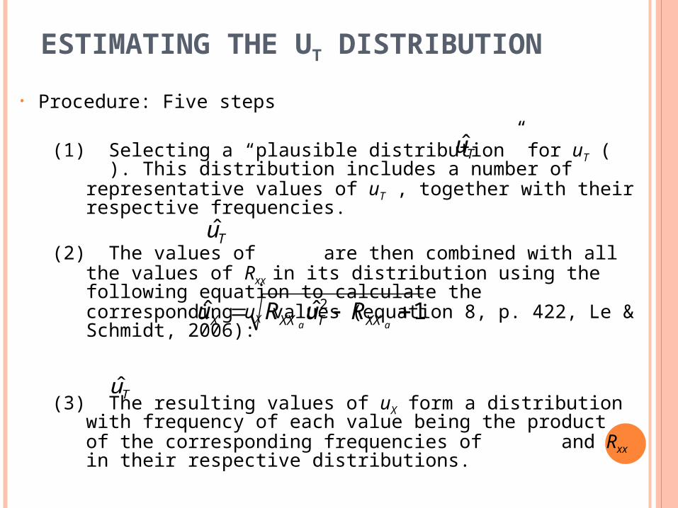
• Procedure: Five steps

(1) Selecting a “plausible distribution” for uT ( ). This distribution includes a number of representative values of uT , together with their respective frequencies.

(2) The values of are then combined with all the values of Rxx in its distribution using the following equation to calculate the corresponding uX values (equation 8, p. 422, Le & Schmidt, 2006):

(3) The resulting values of uX form a distribution with frequency of each value being the product of the corresponding frequencies of and Rxx in their respective distributions.

1ˆˆ 2 aa XXTXXX RuRu

Tu

Tu

Tu

ESTIMATING THE UT DISTRIBUTION

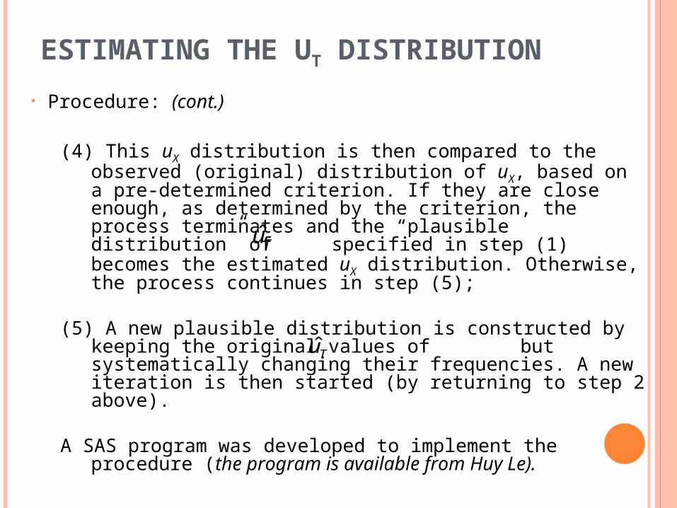
• Procedure: (cont.)

(4) This uX distribution is then compared to the observed (original) distribution of uX, based on a pre-determined criterion. If they are close enough, as determined by the criterion, the process terminates and the “plausible distribution” of specified in step (1) becomes the estimated uX distribution. Otherwise, the process continues in step (5);

(5) A new plausible distribution is constructed by keeping the original values of but systematically changing their frequencies. A new iteration is then started (by returning to step 2 above).

A SAS program was developed to implement the procedure (the program is available from Huy Le).

Tu

Tu

ESTIMATING THE UT DISTRIBUTION Demonstration of the procedure:

• Note that the uX distribution for cognitive tests derived by Alexander et al. (1989) and the Rxxa distribution derived by Schmidt and Hunter (1977) were used.

RESULT: THE UT DISTRIBUTION FOR COGNITIVE MEASURES

Alexander et al. (1989)’s Distribution of uX

(Cognitive)

Estimated Distribution of uT

uX FrequencySelection

RatiouT Frequency

SelectionRatio

1.00 .05 100% 1.00 .05 100%.849 .15 90% .807 .13 85.8%.766 .20 80% .710 .15 71.4%.701 .20 70% .632 .17 56.5%.649 .20 60% .562 .18 41%.603 .15 50% .499 .29 26.6%.599 .05 40% .432 .03 13.3%

=.718; = .107 (Skewness =0.80; Kurtosis = 0.33)

=.628; = .139 (Skewness = 0.94; Kurtosis = 0.36)

XuXuSD Tu

TuSD

RESULT: THE UT DISTRIBUTION FOR EDUCATIONAL TESTS

Alexander et al. (1989)’s Distribution of uX

(Education)

Estimated Distribution of uT

uX FrequencySelection

RatiouT Frequency

SelectionRatio

.849 .15 90% .807 .11 85.8%

.766 .20 80% .710 .15 71.4%

.701 .20 70% .632 .23 56.5%

.649 .20 60% .562 .23 41%

.603 .15 50% .499 .23 26.6%

.599 .05 40% .432 .05 13.3%

=.704; = .084 (Skewness =0.28; Kurtosis = -0.84)

=.607; = .105(Skewness = 0.43; Kurtosis = 0.69)

XuXuSD Tu

TuSD

DISCUSSION• Procedures to correct for indirect range

restriction are necessarily complicated, but the procedure described in this paper will allow better, more accurate estimation of the uT distribution More accurate meta-analysis results.

• The uT distributions estimated here can be used by researchers in their future research.

• Alternatively, meta-analysts can apply the current procedure to any situations where there are only sparse information about range restriction and reliabilities in their data (i.e., primary studies).

THANK YOU!

Any Questions or Comments?