cabi working paper 6 final

KNOWLEDGE FOR LIFE

CA

BI W

OR

KIN

G P

AP

ER

6

October 2013

Impact Evaluation of Plant Clinics: Teso, Uganda

AuthorsJosh Brubaker Solveig Danielsen Max Olupot Dannie Romney Nathan Ochatum

ThInt(rethe

ThCohtt

Thex

BruTe

JosAs

SoEv

MaAg

Da

NaCo

is study and ernational D

esearch grane views of tho

e copyright hommons Attrip://creativec

is working paperience. It

ubaker, J., Dso, Uganda.

sh Brubaker ssistant, LEA

olveig Danielsvaluation, bas

ax Olupot (mgricultural Ad

annie Romne

athan Ochatuonsultant, Ug

the preparaevelopment t no. 09-022ose organisa

holder of thisibution-Noncommons.org

aper was extmay be refe

Danielsen, S. CABI Worki

(jbrubaker@AD Analytics,

sen (s.daniesed in the Ne

molupot@afaavisory Servic

ey (d.romny@

um (nathelaoganda.

tion of the wand the MinDBL), with inations and is

s work is CABcommercial Lg/license/.

ternally peerrred to as:

, Olupot, M.,ing Paper 6,

@leadanalyticInc., Washin

[email protected] (p

as-africa.orgces, Uganda

@cabi.org) is

okwii@yahoo

working paperistry of Forein-kind contribthe sole wor

B InternationLicence (CC

r-reviewed by

Romney, D88 pp.

csinc.com) isngton, DC;

org) is CABI’spreviously Un

or maxolupo;

CABI’s Glob

o.co.uk or na

r was financiign Affairs ofbution by AFrk of its auth

nal (trading aBY-NC). For

y an impact e

. and Ochatu

s an indepen

s Plantwise Pniversity of C

[email protected]

bal Director,

thela2010@

ially supportef Denmark thAAS. Howevors.

as CABI). It isr further deta

evaluation sp

um, N. (2013

dent Impact

Programme CCopenhagen)

o.uk) is a Te

Knowledge

@gmail.com) i

ed by the UKrough the Un

ver, it does n

s made availaails please re

pecialist with

3) Impact eva

Evaluation C

Co-ordinator);

chnical Assis

for Developm

s an indepen

K Departmenniversity of C

not necessari

able under aefer to

h wide interna

aluation of pl

Consultant a

r, Monitoring

stant, African

ment, based

ndent Data M

t for Copenhagen ily represent

a Creative

ational

ant clinics:

nd Research

and

n Forum for

in Kenya;

Management

h

t

CA

BI W

OR

KIN

G P

AP

ER

6

Impact Evaluation of Plant Clinics: Teso, Uganda

Josh Brubaker, LEAD Analytics, Inc.

Solveig Danielsen, formerly University of Copenhagen (now CABI)

Max Olupot, African Forum for Agricultural Advisory Services

Dannie Romney, CABI

Nathan Ochatum, Uganda

Donors

An output of

Plantwise is a global programme, led by CABI, to increase food security and improve rural livelihoods by reducing crop losses.

1

Table of Contents

Table of Contents ................................................................................................................................................................ 1

Abstract .............................................................................................................................................................................. 3

1. Overview ......................................................................................................................................................................... 4

2. Identifying impact ........................................................................................................................................................... 5

3. Data ................................................................................................................................................................................. 7

3.1 Sampling strategy ..................................................................................................................................................... 7

3.2 Household survey ..................................................................................................................................................... 8

3.3 Independent variables .............................................................................................................................................. 9

3.4 Dependent variables ............................................................................................................................................... 11

3.5 Orange producer characteristics ............................................................................................................................. 14

3.6 Cassava producer characteristics ............................................................................................................................ 17

3.7 Expected impacts of plant clinic attendance .......................................................................................................... 20

4. Methodology ................................................................................................................................................................ 21

4.1 Difference in difference .......................................................................................................................................... 21

4.2 Propensity score matching with difference in difference ....................................................................................... 22

4.3 Inverse propensity weighting.................................................................................................................................. 26

5. Results ........................................................................................................................................................................... 26

5.1 Orange producers ................................................................................................................................................... 26

5.2 Cassava producers .................................................................................................................................................. 29

5.3 Summary of impact findings ................................................................................................................................... 31

6. Programme function ..................................................................................................................................................... 31

6.1 Plant clinic user characteristics ............................................................................................................................... 31

6.2 Input availability ..................................................................................................................................................... 38

6.3 Plant clinic recommendations................................................................................................................................. 47

7. Challenges and lessons learned .................................................................................................................................... 50

7.1 Evaluation design .................................................................................................................................................... 50

7.2 Survey design .......................................................................................................................................................... 53

7.3 Suggestions for improvement ................................................................................................................................. 56

8. Conclusion..................................................................................................................................................................... 59

Acknowledgements .......................................................................................................................................................... 60

References ........................................................................................................................................................................ 61

Acronyms .......................................................................................................................................................................... 64

Appendix 1 ........................................................................................................................................................................ 65

2

Figures

Fig. 1. Density and geographic distribution of plant clinic users in Teso region. Each dot indicates one user. The

individual plant clinics are shown with different colours. Users living in Bukedea were not included. ............................. 8

Fig. 2. Sources where plant clinic users heard of the plant clinic. .................................................................................... 32

Fig. 3. Non-user producers who had heard of the plant clinics stated reason(s) for not attending. ................................ 33

Fig. 4. Non-users’ method(s) of verifying plant health problems. .................................................................................... 34

Fig. 5. Sources of plant problem information other than plant clinics, by plant clinic user status. ................................. 35

Fig. 6. Sources where producer bought pesticide by year and plant clinic user status. ................................................... 40

Fig. 7. Reason(s) producer did not buy pesticide by year and plant clinic user status. .................................................... 41

Fig. 8. Sources where producer bought fertilizer by year and plant clinic user status. .................................................... 42

Fig. 9. Reasons producer did not buy fertilizer by year and plant clinic status. ............................................................... 43

Fig. 10. Sources where producer bought planting material by year and plant clinic user status. .................................... 44

Fig. 11. Reasons producer did not buy planting material by year and plant clinic user status. ....................................... 45

Fig. 12. Credit source(s) in 2011 by plant clinic user status. ............................................................................................. 46

Fig. 13. Reason(s) for ‘major crop failure’ by year and plant clinic user status (HH = household). .................................. 47

Tables

Table 1a. Differences in means for orange producers. ..................................................................................................... 15

Table 1b. Orange producer problems experienced. ......................................................................................................... 16

Table 2a. Differences in means for cassava producers. .................................................................................................... 18

Table 2b. Cassava producer problems experienced. ........................................................................................................ 19

Table 3. Orange producer probability of attending a plant clinic. .................................................................................... 24

Table 4. Cassava producer probability of attending a plant clinic. ................................................................................... 25

Table 5. Impact of plant clinic attendance on orange producers. .................................................................................... 27

Table 6. Impact of plant clinic attendance on cassava producers. ................................................................................... 30

Table 7. Percent of respondents using alternative information sources for plant problems. .......................................... 36

Table 8. Percent of households that received information on plant problems by source. .............................................. 37

Table 9. Characteristics of the household member who attended a plant clinic (n = 204). ............................................. 37

Table 10. Differences in input availability by plant clinic user status. .............................................................................. 39

3

Abstract

This CABI Working Paper uses quasi-experimental data to test for changes in orange producer input costs, yield and profitability attributable to plant clinics operating in the Teso region of Uganda. Methods used include producer fixed effects difference in difference regression; propensity score matching with difference in difference; and inverse propensity weighted producer fixed effects difference in difference estimation of impact. The tests find some evidence of lower yields and revenue for farmers visiting the plant clinic, and some suggestion of increased expenditures on labour. Potential explanatory factors for the decline in yield and revenue are discussed. The paper also presents data gathered on a number of contextual questions pertinent for the continued operation and improvement of the plant clinic programme. Finally, the paper discusses challenges for this impact evaluation and makes recommendations to improve future impact evaluations in the areas of evaluation design and survey design, and suggests ways to ensure better plant clinic functioning.

4

1. Overview

In 2005 and 2006, plant health clinics were established in Mukono, Iganga and Soroti districts of Uganda as a novel way to provide plant health advice to farmers. Early results showed that the plant clinics had the potential to enhance the outreach of agricultural extension, capture wider farmer demand and improve disease vigilance. Recognizing this potential, the Ministry of Agriculture, Animal Industry and Fisheries (MAAIF) included plant clinics in the 5-year Development Strategy and Investment Plan (DSIP) as part of the approach taken by the Pest and Disease Control Sub-programme (Danielsen et al., 2012).

After a period of inactivity, the plant clinics were reactivated in 2010 under the guidance of MAAIF and CABI as part of the Plantwise programme. During 2010 and 2011, plant clinics were run in 13 districts by local governments (LGs) and non-governmental organizations (NGOs), with additional districts showing interest in joining the initiative. There was a growing commitment among implementers and policy makers to expand and consolidate these services. In the Teso region there were a total of seven plant clinics operational from June 2010 to September 2011, serving Serere, Soroti, Kumi, Ngora and Bukedea districts. Although the plant clinics were not running regularly, a total of 589 farmers visited them and received advice during that period.

The plant clinics represent an innovative delivery method for agricultural extension services to help farmers to deal with plant pests and diseases and other problems. The plant clinics in Teso were intended to operate in essentially the same way as plant clinics operating in Bolivia (Bentley et al., 2009, 2011) and Bangladesh (Harun-Ar-Rashid et al., 2010). The mandate and long-term vision for these plant clinics was broad, encompassing provision of advice on any aspect of plant production. However, in practice the plant clinics focused primarily on diagnosing and giving advice on how to deal with plant health problems. Common advice pertaining to plant health problems often includes selecting varieties and other inputs that improve plant health and vitality. In the short run this type of advice will increase plant resistance to problems and help mitigate losses. In the long run, this may lead to increased profitability through increasing yields leading to greater quantity sold and/or improving quality leading to better terms of sale. The primary questions that the impact analysis seeks to answer are whether the plant clinics caused changes in production costs, yields and overall profitability for orange producers.

The time span between advice given to cassava producers and data collection was too short to reasonably expect plant clinic attendance to have caused any changes in analysis outcomes. This was because in the majority of cases the problems brought to clinics were viral diseases, for which there is no treatment, and advice focused on using clean materials and resistant varieties in the next season. Although this meant that the data for cassava producers were not useful for this impact analysis, it was thought that robustness checks could still be performed on the data to check their suitability for future use. Because impacts for the treated group were not expected, it was thought that tests of differences in outcomes due to participation would be insignificant if the comparison group represented a reliable counterfactual to the treated group. The same tests that were run to find impacts attributable to the plant clinics for orange producers were used for this robustness check on the cassava producer data.

The Plantwise programme to scale up and expand plant clinics was established in 2011, building on previous experiences from activities in Uganda and elsewhere under the former Global Plant Clinic. A key part of any large development initiative is monitoring and evaluation that can inform effective programme management. Assessing programme impacts and learning lessons are essential to adapt and improve implementation. The present paper describes a study that developed a methodology to assess the impact of plant clinics using activities in the Teso region of Uganda as a case. This study was a collaborative effort of CABI, the University of Copenhagen, and the African Forum for Agricultural Advisory Services (AFAAS).

The remainder of the paper is organized as follows: Section 2 discusses the strategy used to identify impact; Section 3 describes the data collection process and discusses the characteristics of the treated and comparison groups; Section 4 outlines the econometric methods used; Section 5 presents and discusses results of the impact analysis; Section 6 analyses information about market conditions faced by producers, and questions related to programme efficacy; Section 7 comments on the impact evaluation process and provides suggestions for improvement of future impact evaluations; and Section 8 provides a conclusion.

5

2. Identifying impact

The fundamental challenge of describing the impact of the plant clinics is to reliably estimate what would have happened to the participants if the programme had not occurred. A participant’s outcome in the absence of the intervention is its counterfactual. The problem is that while it is necessary to compare actual and counterfactual outcomes in order to assess a programme’s impact, the counterfactual outcome is never observed. Therefore, the challenge is to define the counterfactual. To approximate this counterfactual, this evaluation will construct a comparison group that is as statistically similar to the participant group as possible. The participant group will be referred to hereafter as treatment or plant clinic users, while the non-participant group will be referred to as comparison or non-users. The outcomes for the comparison group represent the best available approximation of what would have happened to the treated group in the absence of the plant clinics, given the data. The difference in the outcomes of the treated and comparison groups can therefore be thought of as the programme’s impact.

To our knowledge, no rigorous impact evaluations of directly analogous programmes have been conducted. The plant clinics represent an innovation in the delivery of extension services in the Ugandan context in both method and purpose. Studies have been conducted to try to establish outcomes for plant clinic users in Bolivia (Bentley et al., 2011) and Bangladesh (Harun-Ar-Rashid et al., 2010). Both studies, and the Bolivian case in particular, showed strong positive effects due to plant clinic participation. However, neither study incorporated a counterfactual group, which means that the results do not control for the possibility of self-selection bias affecting treated producers’ outcomes in addition to causing them to attend plant clinics. There is a rich literature on the subject of agricultural research and extension, which is relevant to this study. Birkhaeuser et al. (1991) review evidence from 48 studies on the benefits of agricultural research and extension, and found that 36 of these studies reported strong positive impacts on productivity, knowledge and adoption attributed to extension. Alston et al. (2000) present a meta-review of rates of return for a wide variety of agricultural research related projects. They focus on rates of return as a reasonably comparable indicator across these programmes, which varied widely in design and purpose. They find generally positive rates of return, but fairly wide variance in those rates of return. Anderson (2007) provides an update to Alston et al. by expanding on extension-specific literature. Anderson highlights a variety of measurement issues relevant to evaluating extension work, and notes that the more recent data-intensive evaluation work has found mixed results for extension in terms of return on investment. Davis (2008) reviews extant evidence on farmer field schools in sub-Saharan Africa and highlights a lack of strong evidence of impacts that can definitely be attributed to extension programmes.

The National Agricultural Advisory Services (NAADS) programme of Uganda was operating in Teso during the time period studied here. NAADS focuses on farmer groups, and is involved in a wide range of activities including directly distributing and/or subsidizing key inputs. Benin et al. (2011) evaluated the impact of NAADS on total agricultural revenue per adult equivalent at the household level, and found a significant positive impact from 32% to 63% between 2004 and 2007. There are some concerns about the comparison due to NAADS’ focus on poorer farmers and the resulting differences between the treated and comparison groups available for the analysis. In summary, agricultural extension projects generally can have strong and positive impacts on producer outcomes, but estimates also reveal fairly high variance and are plagued by a number of measurement and attribution problems.

A central concern in evaluating the plant clinics is the problem of selection bias. Farmers chose for themselves whether to attend the plant clinics. This presents the possibility that even if there were no other observed differences between the treatment and comparison groups, there was still a fundamental difference between the groups, because one chose to attend a plant clinic and the other did not. It is possible that the type of farmer who chose to attend a plant clinic has some unobserved characteristic, which non-users did not have. If this is true, the unobserved characteristic might also have an effect on the outcomes of interest. A simple ordinary least squares (OLS) regression would not be able to account for this selection bias and could attribute outcomes to the plant clinics that represent a spurious correlation with the unobserved characteristic rather than a true programme impact. The household fixed effects, propensity score matching and inverse propensity weighting methods described in Section 4 will help to overcome this potential source of bias (Imbens and Wooldridge, 2008).

6

One further source of potential bias is referred to as programme placement bias. This refers to the possibility that plant clinics may have been placed in areas that are systematically different from areas that did not have plant clinics, which is of interest in assessing the external validity of the results from this evaluation. The plant clinic locations within the Teso region are in significant market centres. An empirical assessment of potential differences across other regions of Uganda is beyond the scope of this evaluation. Agricultural census data do make it clear that there are noteworthy differences in agricultural practices across the regions of Uganda (UBoS, 2010), so plant clinics will need to adapt to local conditions if they are to scale up nationally. Programme placement bias is not presumed to be a concern for the internal validity of this study due to the relative similarity of the market centres chosen by the programme. To further ensure that any differences based on geography are not a problem, controls for district are included in the vector of characteristics for the estimation of the propensity score, and all impact estimates adjust standard errors to account for any correlation based on which plant clinic the producer lived nearest to.

The plant clinics’ mandate to help any farmer with any crop-related question meant that the potential scope of programme impact was quite wide. In order to narrow the scope of the analysis, a decision was made to focus on cassava and orange, which were the crops brought to the plant clinics most frequently. Cassava is the predominant staple food security crop in the Teso region. Orange is a key cash crop, which farmers can sell relatively easily. Narrowing the evaluation to two crops helped keep the survey length reasonable, which helped mitigate respondent fatigue and thereby improved data quality. One downside is that since plot-level data were only collected for orange and cassava, they do not capture a complete picture of producer practices since most farmers produce five or six crops. Therefore this dataset does not allow generalizations about overall producer profitability. It is reasonable to expect the plant clinics to have a stronger impact at the crop level than at the producer level, since the primary focus of the plant clinics was to help deal with plant problems, which tend to be crop specific.

A relatively wide range of diseases affected both orange and cassava plants (Danielsen et al., 2012, p. 42), which increased the expected variation in programme impact ex ante. As a result, sample size calculations call for a sample that is much larger than that used in this study. Further analysis of sample size and statistical power is presented in Section 7.1.1. Rather than an explicit sample size calculation, the sample size used was determined by the number of treated households available for each crop. Given the small number of producers available for this impact evaluation and the relatively high variance in the impact variables selected, impacts of the plant clinics would have had to be very strong and consistent to be found, which was unlikely.

Time lag before effects are observed is another evaluation problem related to the nature of the plant clinics. Other research on agricultural research related projects often allow for and expect significant time lag prior to final evaluation for effects to be realized (Alston et al., 2000, p. 49; Benin et al., 2008, p. 49). For example, in the plant clinics’ context, curing virus problems in cassava (e.g. brown streak disease, mosaic disease) requires that the plot be uprooted and replanted with resistant varieties. For producers that do take up a recommendation like this, the gains in output will take a full season to become apparent. Other types of advice also have substantial lag times. The surveys did attempt to capture retroactive data, but even so the data only cover two years of crops and one year of treatment, which may be too short to capture the full impact of the programme.

There was potential for leakages from plant clinic operation. When plant clinic users discuss problems and share information with other farmers, advice might leak to untreated households. If spillover effects are occurring, this analysis will understate impact due to its focus on the effect of treatment on the treated. All producers in the Teso region were in the intent to treat (ITT) group, since anyone with a plant problem and access to market centres could have accessed the plant clinics. Future evaluations could focus on ITT, which would entail calculating the effect of plant clinics on all producers in the treatment area compared to similar producers in a similar but untreated area. For future evaluations, focusing on ITT would greatly reduce or eliminate concerns about spillover effects within the treated areas. This study calculates the average treatment on the treated (ATT), or the difference in outcomes between producers who actually took up the treatment by attending the plant clinics and producers who did not attend.

Focusing on ATT leaves open the possibility that treated households could communicate with comparison households and contaminate the counterfactual. If this happens, the comparison households could be receiving programme benefits without attending the plant clinics. The effect of the plant clinics would be diluted if this communication is widespread and comparison households take up the recommendations at similar rates to treated producers. This possibility is seen as insubstantial for this evaluation since the plant

7

clinics had only been running for a short time, and non-treated farmers are likely to be slow to adopt until they see evidence that following plant clinic recommendations does in fact improve outcomes for treated farmers. In addition, plant clinics were providing specific recommendations for specific problems. Theoretically, a comparison producer would need to have the same plant problem and have applied similar counter measures to the treated producer prior to receiving a recommendation for the recommendation to be fully effective. This should minimize any potential leakages from treated to comparison households.

Evaluation of impact will be conducted separately for cassava and orange producers. There are households who produced both cassava and orange, but only took one of the crops to the plant clinic. If a household took a cassava problem to the plant clinic and not an orange problem, they will be considered a treated household for the cassava analysis, and are eligible to be considered as a comparison household for the orange analysis. Plant doctors were trained to give general advice related to good crop hygiene, such as removing infected plants/fruits and sanitizing tools so as to reduce disease transmission. The transferability of this advice between crops is somewhat limited. Any generally applicable advice that was given was not recorded as a formal recommendation in the plant clinic records or in the household survey. The possibility exists that comparison households who produced both crops might have gained spillover benefits from plant clinic attendance, and the methods used do not control for that possibility. There is some potential for spillover between the different treatment groups, which means that the results below may slightly underestimate programme impact. However, this issue is not deemed serious enough to cast doubt on the validity of the results, since the plant clinics provide specific recommendations for specific problems and it is unlikely that advice given for one crop could be beneficial to the other. There were 11 producers, or 13.3% of the cassava treatment group, who were also used as comparison producers (12.5% of the comparison group) for the orange analysis. Seventy-three treated orange producers (83%) were used in the comparison group in the cassava analysis (29.7% of the cassava comparison group).

3. Data

To collect data, a household survey was administered to treatment and comparison households in the Teso region in early 2011. Randomized programme rollout was not feasible for this evaluation. Instead, an attempt was made to focus sampling on populations where the potential self-selection and programme placement biases would be minimized. The dataset is therefore quasi-experimental, and is intended to simulate an experiment as closely as possible.

Plant clinic clients come from many different villages and are widely dispersed (see Fig. 1). A total of 102 cassava clients from 87 villages and 235 orange clients from 190 villages were recorded in the plant clinic record. Comparison areas were selected to represent key areas of variability expected to affect cassava and orange production that could be described spatially at the parish level. These factors included population density, climate, soil type and land use type. Locations were selected to match the distribution of characteristics in treatment areas, rather than trying to find comparison households in every treated village. The purpose of this comparison village selection process was to overcome the potential programme placement bias through targeted sampling in case there is something different about the areas where plant clinics were operating. The areas selected give a good representation of the characteristics present in the Teso region of Uganda and the conditions faced by treated households.

3.1 Sampling strategy

Once the comparison villages had been identified, a secondary screening process was used to ensure that the producers surveyed would form a comparison group as statistically similar to the treatment group as possible. Exit surveys were administered to plant clinic users to establish characteristics of attending households. The specific variables collected included household demographics, household head characteristics, a number of household wealth indicators (e.g. livestock, dwelling characteristics), and geographic location. These results were compiled to make a list of screening questions to be applied during selection of the comparison group. The selection criteria were that the farmer cultivated one of the crops of interest, was between 25 and 65 years of age, and did not exceed specified asset thresholds (land area, livestock, vehicle ownership, electricity in the dwelling). See Section A of Appendix 1 for greater detail. Enumeration teams visited each selected village and selected households at random from the population of households that had been identified by village elders as cultivating orange or cassava. The screening

8

questions were administered to selected households and those that met the selection criteria received the full survey. This screening process was intended to help decrease the sample size required to deal with self-selection bias by targeting comparison households that were as similar as possible to the majority of treated households from the outset.

Most of the comparison producers had been surveyed by mid-February, and the process of finding and surveying the treatment producers began. Treatment producers had to be tracked down based on the name and village they had given in the plant clinic exit survey. This task proved challenging given the large size of villages (100–200 households) specified and the imprecise names given in plant clinic records. Once found, treatment producers were administered a survey very similar to that filled out by comparison producers. Treated producers were asked additional questions about crop problems diagnosed (rather than experienced) to try to capture how well the transmission of plant clinic advice had worked. Some of the producers surveyed did not report any plot-level activity for cassava or orange. Only producers that reported some kind of activity on their plot(s) are considered in the impact analysis.

Fig. 1. Density and geographic distribution of plant clinic users in Teso region. Each dot indicates one user. The individual plant clinics are shown with different colours. Users living in Bukedea were not included.

The dataset also contains records from the survey and the plant clinic record on recommendations made to treated producers. This data subset will be discussed in more detail when the programme evaluation questions are addressed in Section 6 of this paper. To preview this discussion, there was a high degree of discrepancy between the survey description and the plant clinic records of the plant clinic interaction. As such, the recommendation uptake data that were collected were not deemed reliable enough to be included in the impact evaluation.

3.2 Household survey

The household survey instrument was designed by CABI and partners from University of Copenhagen, AFAAS and Makerere University, field tested, and finally approved for use in early 2011. Surveying was

9

postponed until early February to allow farmers to finish the orange harvest, and was mostly completed by March, with a few late results coming in during April. A partner from AFAAS administered the survey, with help from several subcontracted local enumerators. In total, data were collected from 416 households, 205 of which attended a plant clinic and 211 of which did not attend. The data were cleaned and respondents who did not give any production data for the specified crops were excluded. In addition, the sample was restricted to the households that formed a reasonable comparison group (on common support) using the propensity score matching methodology described later in this paper. After data cleaning and imposition of common support the final number of orange producers considered was 189, and the final number of cassava producers was 329.

The surveys included detailed plot-level questions for cassava and orange production in 2011 and retrospectively for 2010. Since measurement occurred after the programme had begun operation, including the 2010 questions was the most practical method to gather data on baseline producer practices. In addition, the surveys asked about a broad range of household characteristics including demographics, education levels, economic activities and physical assets. These data are not true baseline characteristics, which raises the concern that the programme might have had an impact on them. Great care was used in selecting control variables to ensure that the impacts of the programme are not confounded by changes to household characteristics.

Asking farmers for detailed plot-level data from further back than one season is difficult. Farmers may not remember exactly what they did in the previous season, and may lose more precision in their recall as more time elapses. Recall is likely to be particularly problematic with cassava since farmers tend not to keep records for the crop and it can be harvested in small amounts over a long period of time. In short, recall data are likely to be less precise and therefore less reliable for empirical purposes (Iarossi, 2006, pp. 54–58). To help ensure that the retrospective data would be as reliable as possible, the surveys asked detailed questions about farmer practices. For example, in the case of pesticide

1 use, farmers were asked which

pesticide they used on each plot, how much they put into each knapsack sprayer, how many knapsack sprayers they put on the plot per session of pesticide application, and how many sessions they did in a year. The detail of the questionnaire is expected to have increased the precision of farmer recall on the retroactive questions. The reliability of recall data from a previous year remains a significant concern when estimating impact using this dataset, which will be discussed further in Section 7 of this paper.

One problem experienced in this evaluation was the lack of data on the extent to which a particular problem affected producers’ crops and the correlated lack of a clear method to describe the relative quality of practices for their crops. All households were asked which pests and/or diseases they experienced in each crop, but there was no record of the severity of the problem. In addition, no data were collected on the crop problems experienced in 2010. This impact evaluation therefore does not attempt to measure quality of farmer response to their plant problems in the absence of more thorough information on problems experienced. The tests used compare outcomes of producers who attended plant clinics with those who did not. The results of the impact evaluation therefore do not constitute a direct test of the quality of advice given or a test of farmer efficacy at following said advice. It is safe to assume that some comparison producers used better practices in the absence of the plant clinics, and some treated producers did not use better practices in the presence of the plant clinics. The farmers that received plant clinic advice were expected to follow better practices more often, and it was expected that this would lead to improved farmer outcomes. To the extent that this effect occurred, the tests used will capture evidence of the improvement in farmer outcomes resulting from attending a plant clinic and improving their plant problem management practices.

3.3 Independent variables

While this analysis tests whether attending the plant clinics caused changes in recipients’ production decisions, it is likely that plant clinic advice was not the only factor influencing these decisions. Therefore, a vector of covariates was included in the analysis to control for observable characteristics that could have influenced outcomes but that were unlikely to be impacted by plant clinic participation. It is crucial that the covariates not be influenced by plant clinic participation, as this would raise a concern of simultaneous causality, which would bias test results (Stock and Watson, 2011, pp. 324–326). Selection of covariates was

1 Pesticide here and elsewhere in this paper may refer to insecticide, herbicide, or fungicide.

10

based on prior research regarding factors likely to influence producer decision-making (Singh et al., 1986; de Janvry et al., 1991; Feder and Umali, 1993; Epeju, 2010). The full list of control variables used in this analysis can be seen in Tables 1a and 2a in Sections 3.5 and 3.6. Some variables are simple to understand. This section offers descriptions of less straightforward control variables.

A variable representing distance to nearest plant clinic was calculated based on GPS coordinates for the households and GPS coordinates for the plant clinics. The values are an ‘as the crow flies’ number of miles

2.

This variable is considered useful as a control since physical distance from the plant clinic was expected to influence the farmers’ decision about how frequently to visit the market and therefore how frequently they could potentially access the plant clinic with no additional travel cost. The variable should be interpreted with care since it is a very simple way to approximate the cost of producer travel.

Three variables were created to control for producer wealth, which is presumed to affect both production decisions and the choice of whether to attend a plant clinic. An asset index was constructed, which is a weighted aggregate of household assets. The assets considered were the number of radios, transportation related items (bicycle, motorbike, car/pickup), and ox ploughs owned. The weighting system is based on asset scarcity, with higher weights assigned to assets that were less frequently owned. The exact specification for an individual household’s asset score is described in Equation 1. A dwelling index was calculated as a simple sum of three binary variables for three dwelling characteristics (floor, permanent dwelling type and latrine access), such that a value of three indicates a completely upgraded dwelling and zero indicates a basic dwelling. Livestock were included as a single variable aggregated in tropical livestock unit

3 (TLU) terms.

�1�� ∗ �1 ��

� � ��1, ��2, … , �� Where: Ai = asset index of household i aji = number of asset j owned by household i nj>0 = number of households who own any of asset j N = number of households in the sample

An ordinal variable capturing highest level of education completed by any household member was created. The categories include none, primary, and any degree beyond primary including secondary school, technical degrees and university degrees. Education is included as a control variable since more education is presumed to correlate positively with better outcomes generally due to greater capacity to access information and deal with crop problems. Household education is considered rather than head education because it is assumed that information is shared and capacity was pooled to some degree within the household.

Household labour and social capital can be important determinants of uptake of improved agricultural production techniques (Beckmann et al., 2006). A household member is understood here to be an adult if s/he was 15 or more years of age at the time of the survey. Adults who report any kind of economic activity were counted as part of the household’s labour force. Counting the labour force in this way relied on the simplifying assumption that all household labourers are equivalent. Two variables are included to control for off-farm activities by household members. The first captures any type of agricultural labour performed off the household farm, and the second considers any other type of paid labour. These variables are included to control for the possibility that households containing a member with external employment might have different kinds of social capital and/or resources than households where all members are employed only on their own farm. Capturing this element of social capital was important since more of it is expected to correlate with greater capacity to seek out advice and therefore impact on both a household’s likelihood to attend the plant clinics and a household’s outcomes in the absence of plant clinics.

2 Miles were the units used by respondents, so are maintained here to represent the original data most accurately. 1 mile

= 1.61 kilometres.

3 TLU conversion factors used: cattle = 0.7, pigs = 0.2, sheep = 0.1, goats = 0.1, turkeys = 0.02, chickens = 0.01.

11

3.4 Dependent variables

The impact analysis considers cost components, crop yields and aggregate profit per acre4 as dependent

variables. Each variable is considered directly, as well as de-meaned. The dependent variables are described in greater detail below.

3.4.1 Cost variables

Cost variables are considered in this analysis as a proxy for producer decision-making about inputs for their crops. It would be desirable to analyse producer input decisions directly, but the high degree of complexity in the input choices available combined with the small sample size meant that this was not practical. Considering the case of pesticide, focusing on cost per acre is a simplified way to study producer pesticide practices, which could vary due to changing varieties or concentrations of pesticide being applied. Focusing on cost relies on the assumption that if producers are changing their practices there will be an impact on the amount of money they spend on the input per acre. The trade-off is the results will not definitively illuminate whether the changes are in quantity (application rate) or quality (type) of input used. The cost variables considered for both crops are pesticide, fertilizer, planting materials (cuttings for cassava and seedlings for orange) and labour. The pesticide variable used captures insecticide, herbicide and fungicide. It does not capture items like ash, which is traditionally applied to help manage pests, but is not traded and therefore did not have useful price information and so was excluded from the analysis.

5 Fertilizer captures both mineral

and organic fertilizer. Manure and other types of organic fertilizer are often sourced from the producers’ own farm, but also traded enough for the price information to be more reliable.

The process for generating the pesticide, fertilizer and planting material variables is generalized in Equation 2 below. The case of pesticide for orange producers is taken as an example and described here. To ascertain the amount of pesticide used per year, respondents were asked how much pesticide they used per application unit (e.g. per knapsack sprayer), how many application units were used per application session, and how many application sessions were conducted per year. Note that this process assumes that all application sessions were equal, which may not necessarily be true. Therefore the variables represent the farmers’ best estimates rather than definite records.

�2�� ∗ �� ∗ �� ∗ �!��"��#�

Where yit = cost per acre of pesticide applied for household i in year t nait = number of units of pesticide per application unit* ait = application units per application session sit = application sessions per year pit = price per unit of pesticide uit = units in which pesticide is purchased* qi = acres under cultivation (by crop) * The survey asked for the amount that the producer used and purchased separately, which were converted to the amount of a single common unit for this calculation.

To calculate the cost of the amount of pesticide applied, farmers were asked what unit of pesticide they bought, and what the cost in Ugandan shillings (USH) was per unit. Units were converted to millilitres in the case of liquid pesticide and kilograms in the case of dry pesticides. The cost per unit was calculated and used to assign a value to the total amount used. These values were then converted to 2011 USH, and converted from there to 2011 USD purchasing power parity (PPP) to increase ease of interpretation for an

4 Acres were the units used by respondents, so are maintained here to represent the original data most accurately. 1

acre = 0.405 hectares.

5 Two producers mentioned using ash. The actual usage of ash is believed to be more common than this low rate of

response indicates. Ash is a widely available natural byproduct generated by producer households. However, enumerators were not instructed to capture this type of pesticide, and producers may not have thought to mention it.

12

international audience6. Inflation was low in 2010 in Uganda (around 4%), but making these conversions

helps to ensure that the changes being captured by this analysis were due to changes in producer behaviour rather than exogenous changes in price due to inflation. To make the variable comparable across farmers, the total USD cost was divided by the number of acres planted with the specified crop. Many orange farmers gave crop area in terms of trees, so a conversion factor of 140 trees per acre was used to change trees to acres. All land quantities were held fixed at the levels given in Section A7 of the survey (see Appendix 1). The responses from this section were deemed more reliable than the responses in Section E1 due to the lower number of missing responses and fewer outliers. All variables capturing a monetary value are expressed in terms of 2011 USD PPP per acre. Pesticide and fertilizer use were so infrequent for cassava producers that once the process in Equation 2 was complete, a binary was created equal to one if the household reported any value at all, and tests were run on the binary only. These tests showed no impact due to the treatment and are not reported. Costs incurred for pesticide and fertilizer were included in the total cost variable for cassava.

The labour cost variable for cassava producers is the sum of the value of labour spent on weeding, removing infected plants and harvesting. Labour for orange producers is the sum of the value of labour spent spraying, weeding, pruning, removing infected fruits and harvesting. The labour cost of planting is not considered here since it was not collected in the survey for either crop. Respondents reported the number of hours per day spent per person on the task, the number of persons per day and the number of sessions per year. Producers were asked what they pay for a day of labour on each task, and how many hours would be in a hired day on that task. Producers do not necessarily participate in labour markets but they were asked to make an estimate of what they would have to pay if they were to hire labour. From these estimates, an hourly wage rate was calculated for each task for each household. The total value for the separate labour types was added together and divided by the acres on which the crop was being produced in order to increase comparability. It is important to note that many producers are not paying out of pocket for all of the labour used on their crops. This measure is therefore assigning a value to all the labour reported and does not describe actual labour costs paid.

Some respondents did not give price estimates, but did report using one of the cost variables. This response could arise from households borrowing the input or having some other informal arrangement rather than paying directly, and therefore not having a price to report. The issue made up no more than 5% of the observations for any variable, and with no clear difference between treated and comparison households. A price per unit was imputed for these households in order to use as much of the sample as possible. To do the imputations, an OLS regression was run on the price per unit for the specified product or task, excluding values greater than three standard deviations from the mean and controlling for price variation at the district level. The model used to estimate the wage rate is specified in Equation 3 below as an example. In this model, ß0 is an intercept term capturing the wages for the excluded district Ngora (the most frequently represented district in the sample). The other ß terms capture the differences in wages in the specified districts, and µ is an error term capturing all variation not explained by the model. This model was run for other missing cost variables, but including controls for the specific type of product used where appropriate (e.g. type of pesticide, variety of seed). Using the results of this test, a price estimate was assigned to households with missing cost per unit and non-missing number of units used. The households’ values were calculated using the imputed prices in the same way described in Equation 2 above for households with non-missing prices. �3�%&�� ß� ( ß�)"*+� ( ß,-�.�.�� ( ß/-0.0�+� ( μ� Where wlit = hourly wage for labour type l for household i in year t

The aggregate cost variable is a simple sum of the total costs for each input, divided by the total number of acres under cultivation for the crop. It is expected that the plant clinic intervention will cause an increase in costs due to the need for a greater quantity and higher quality of inputs to deal with plant problems.

6 Conversion rates used were from the World Development Indicators online resource maintained by the World Bank.

They can be accessed at http://databank.worldbank.org/data/home.aspx. The 2011 USD PPP/2011 USH conversion factor was 1/1150.689707.

13

3.4.2 Yield variables

Yield variables were compiled in a similar manner to cost variables. Cassava tuber output is considered here as an example. When cassava is harvested the raw tubers are commonly processed into chips, which can be stored and ground into cassava flour. To make chips, tubers are peeled and dried, which reduces their weight and volume significantly. When asked about cassava output, some producers expressed their cassava output in chips and others used tubers. To convert chips to tubers, a conversion factor of 1 kg of chips equal to 2 kg of tubers was used. The surveys asked about both harvest and consumption of tubers (either within-household consumption or sale). This analysis uses consumption rather than harvest to focus on the amount that was actually used or sold, since disease or pest pressure could have rendered some harvest unusable. The output of tubers was the sum of tubers and chips (converted to tubers) produced that were consumed. To convert output to yield the quantity of cassava tubers produced was divided by the number of acres where cassava was cultivated. The definition of yield used for cassava tubers is specified in Equation 4 below.

�4�3�� 45�� ( 2 ∗ 65�� ( �47�� ( 2 ∗ 65��#�

Where Yit = yield of cassava tubers for producer i in year t bsit = kg of tubers sold csit = kg of chips sold bcit = kg of tubers consumed ccit = kg of chips consumed qi = cassava area under cultivation

The remaining yield variables considered are cassava cuttings, orange seedlings and orange fruits. The method used to calculate these variables is essentially the same as outlined for tubers above, except that no conversion from chips to tubers was required. Cuttings of cassava come from the plant stem and are used as planting material for new cassava crops. Cuttings are an important form of output and a potential secondary source of revenue for cassava producers. Cutting yield was presented in terms of kilograms harvested per year. Orange fruit harvest happens twice a year, so the values for each year are aggregates of two different seasons’ values. Fruit yield is presented in terms of kilograms per year. Orange seedlings are young orange trees, which households can plant or sell as a secondary source of revenue. Seedling yield is calculated in numbers of seedlings per acre.

Direct analysis of output is done in terms of quantity produced per acre. This method is based on the assumption that type and quality of output are more comparable across the region than values of output, which will be affected by price variation. Direct analysis of cost factors is conducted in terms of value per acre because there is greater variation in the type and quality of the inputs used, making cost the most reasonable common comparison within each category.

To calculate producer profitability, output consumed was converted into revenue per acre. Producers were asked what price they received per unit of tubers sold and this value was converted to the price per kilogram for tubers. Where households consumed some of their own cassava but did not sell any, they were still asked for an estimated price if they had sold their output. In some cases respondents did not give a price estimate, so a price was imputed for these households using the same method that was used to impute wage rates modelled in Equation 3 above. The value of tuber production was computed by multiplying the household’s quantity of output (numerator in the right side of Equation 4 above) by the given price, or the imputed price for households where a price was not given. The value of tuber production is added to the value of cutting production. This value was then divided by the quantity of acres under production for cassava. For orange, fruit and seedling output were multiplied by the appropriate prices. There is some price and quantity variation between the two orange seasons, so the yearly aggregation is done in terms of value rather than quantity to ensure comparability. Where price imputations were necessary, appropriate seasonal prices were used rather than a yearly price.

3.4.3 De-meaned variables

The dependent variables are all considered both directly and as de-meaned variables. Converting an output variable to a de-meaned variable is a two-step process. The first step is to subtract the mean of the variable

14

from each household’s value for that same variable. This means that the mean of the new variable will be approximately equal to zero.

7 The second step is to divide the result of the first step by the standard

deviation of the original variable. Doing so makes the standard deviation of the new variable equal to one. This allows the results for de-meaned variables to be understood in terms of standard deviations from the mean. The results for the de-meaned variable are therefore the most readily comparable to other research. The de-meaning process also helps to normalize the variable, which helps ensure that the OLS assumption of no extreme outliers holds. The de-meaning method and characteristics of the resulting de-meaned variables are described in Equation 5 below:

�5�3�,9: � 3� 3;<= �. �.3;9: ? 0<=AB � 1

Where: i refers to producer i DM indicates variable is de-meaned

3.5 Orange producer characteristics

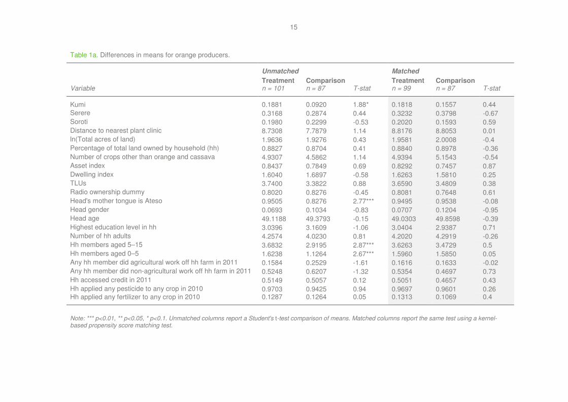
The orange analysis considers 188 orange producers, of which 101 were treated and 87 were comparison. Table 1a presents tests of the differences in means between the treated and comparison households for a range of key characteristics. It is thought that these characteristics could influence plant clinic uptake and production decisions, but that plant clinic uptake would not affect these characteristics. If the sampling strategy were perfectly successful at finding a counterfactual group, no significant differences between the characteristics of the two groups would be seen. Note that two tests are reported for each variable. The unmatched test is a Student’s t-test on the entire sample, while the matched test is a Student’s t-test performed only on the sample remaining after using propensity score matching to ensure that the treatment is compared with the most reasonable comparison group available. The propensity score matching method is explained more thoroughly in Section 4 below.

According to the unmatched Student’s t-tests, four significant differences between characteristics of the treatment and comparison orange producer groups exist when considering the entire sample. The treated group was more likely to be from Kumi and to speak Ateso, and had more children aged 0–5 and young people aged 5–15. These observed differences mean that a simple test for impact might give biased estimates. The fixed effects model described in Section 4 will control for any time invariant differences between the treatment and comparison group in order to account for any potential bias resulting from these differences. For Student’s t-tests conducted on the treatment and the comparison group created using the matching method, all of these significant differences disappear. This means that the matching method was able to successfully find a reasonable counterfactual group and will therefore be able to give unbiased estimates of impact.

The tests in Table 1a do not check whether the pest and disease burdens experienced by the treated and comparison producers differed. The sampling strategy used attempted to find producers with similar risk factors for plant problems such as climate and soil type. To assess whether pest and disease burdens were comparable between the two groups, both treated and comparison producers were asked which problems they had experienced by crop in either 2010 or 2011. The questions were asked slightly differently for the two groups. Treated producers were asked what plant problems they brought to the plant clinic. Comparison producers were asked what plant problems they experienced on their farms. In practice, the treated producers preferred to talk about the problems they were currently experiencing, and many of these were also included in the responses recorded. Plant problems cannot be used as control variables because they can directly cause changes in the output variable itself, and so would confound the results of the impact tests.

7 In practice, the de-meaned variables mean is not precisely zero, but a very small value. As the sample size approaches

infinity, the mean value of a de-meaned variable would be equal to zero.

15

Table 1a. Differences in means for orange producers.

Unmatched Matched

Treatment Comparison Treatment Comparison Variable n = 101 n = 87 T-stat n = 99 n = 87 T-stat

Kumi 0.1881 0.0920 1.88* 0.1818 0.1557 0.44

Serere 0.3168 0.2874 0.44 0.3232 0.3798 -0.67

Soroti 0.1980 0.2299 -0.53 0.2020 0.1593 0.59

Distance to nearest plant clinic 8.7308 7.7879 1.14 8.8176 8.8053 0.01

ln(Total acres of land) 1.9636 1.9276 0.43 1.9581 2.0008 -0.4

Percentage of total land owned by household (hh) 0.8827 0.8704 0.41 0.8840 0.8978 -0.36

Number of crops other than orange and cassava 4.9307 4.5862 1.14 4.9394 5.1543 -0.54

Asset index 0.8437 0.7849 0.69 0.8292 0.7457 0.87

Dwelling index 1.6040 1.6897 -0.58 1.6263 1.5810 0.25

TLUs 3.7400 3.3822 0.88 3.6590 3.4809 0.38

Radio ownership dummy 0.8020 0.8276 -0.45 0.8081 0.7648 0.61

Head's mother tongue is Ateso 0.9505 0.8276 2.77*** 0.9495 0.9538 -0.08

Head gender 0.0693 0.1034 -0.83 0.0707 0.1204 -0.95

Head age 49.1188 49.3793 -0.15 49.0303 49.8598 -0.39

Highest education level in hh 3.0396 3.1609 -1.06 3.0404 2.9387 0.71

Number of hh adults 4.2574 4.0230 0.81 4.2020 4.2919 -0.26

Hh members aged 5–15 3.6832 2.9195 2.87*** 3.6263 3.4729 0.5

Hh members aged 0–5 1.6238 1.1264 2.67*** 1.5960 1.5850 0.05

Any hh member did agricultural work off hh farm in 2011 0.1584 0.2529 -1.61 0.1616 0.1633 -0.02

Any hh member did non-agricultural work off hh farm in 2011 0.5248 0.6207 -1.32 0.5354 0.4697 0.73

Hh accessed credit in 2011 0.5149 0.5057 0.12 0.5051 0.4657 0.43

Hh applied any pesticide to any crop in 2010 0.9703 0.9425 0.94 0.9697 0.9601 0.26 Hh applied any fertilizer to any crop in 2010 0.1287 0.1264 0.05 0.1313 0.1069 0.4

Note: *** p<0.01, ** p<0.05, * p<0.1. Unmatched columns report a Student's t-test comparison of means. Matched columns report the same test using a kernel-based propensity score matching test.

16

Table 1b. Orange producer problems experienced.

Unmatched Matched


Leaf miner 0.4059 0.2989 1.53 0.4040 0.3173 1.01

Fruit fly 0.1683 0.2184 -0.87 0.1717 0.1558 0.22

Aphids 0.4356 0.2989 1.94* 0.4242 0.2160 2.41**

Citrus black spot 0.1089 0.1609 -1.04 0.1111 0.1100 0.02

Orange dog fly 0.0693 0.1379 -1.56 0.0707 0.1171 -0.77

Caterpillars 0.0495 0.0920 -1.14 0.0505 0.0611 -0.21

Scab 0.2574 0.2529 0.07 0.2626 0.2358 0.34

Scale 0.1485 0.1264 0.44 0.1414 0.0903 0.84

Tristeza 0.0297 0 1.62 0.0303 0 1.75* Number of problems 1.6733 1.5862 0.48 1.6667 1.3033 1.49

Note: *** p<0.01, ** p<0.05, * p<0.1. Unmatched columns report a Student's t-test comparison of means. Matched columns report the same test using a kernel-based propensity score matching test

17

Direct tests for significance of the differences in the plant problems experienced by treated and comparison producers are presented in Table 1b. The tests used are the same as those presented in Table 1a. Treated producers were about 46% more likely to report aphid problems with their oranges using the unmatched test, and about 96% more likely to report aphid problems using the matching method. The difference was statistically significant at the 90% confidence level with the unmatched test, and increased in significance to the 95% confidence level with the matching method. This difference is a concern for the impact evaluation, since it means that aphids might systematically impact treated producers’ outcomes. One possible source of this difference is misidentification in the data collection process. Comparison producers reported higher rates of fruit fly and orange dog fly, both of which may be referred to with the word ‘eliana’, which is an Ateso word referring to small flying bugs as a group. It is possible that the difference is due to translation confusion. Data are not available on the severity of problems experienced, so it is not possible to empirically assess the impact of the difference in aphid prevalence, but it is known that aphid infestation alone would have to be severe to cause real losses in orange production (Salem and Hamdy, 1986). The difference in aphid prevalence is expected to bias fruit yield and revenue results down slightly, and might bias pesticide costs up slightly if producers applied more to deal with aphid problems. The treated producers also had a significantly higher rate of tristeza infection using the matching test. There were three treated producers reporting tristeza, and no comparison producers. Tristeza is a viral disease, and may be difficult for producers to diagnose without specialized assistance. The disease can be very destructive (Roistacher and Moreno, 1991), so the significance of the difference is a concern for the impact evaluation. Aphids are a vector for tristeza, and all three producers reporting tristeza also reported aphids, so it is reasonable to assume that these producers are experiencing extraordinary plant problem levels, which might bias the fruit yield and revenue results lower, and possibly bias the labour and planting material cost results higher. The small number of producers reporting tristeza as a problem suggests that any change in impact should be relatively small. Finally, the total number of problems reported was about 5% higher for treated producers in the unmatched sample, and became about 28% higher using the matched sample. The difference using the matched sample was not statistically significant, but is still high enough to be a concern. It is assumed that treated producers having a somewhat higher number of problems on average will bias the yield and revenue results downward.

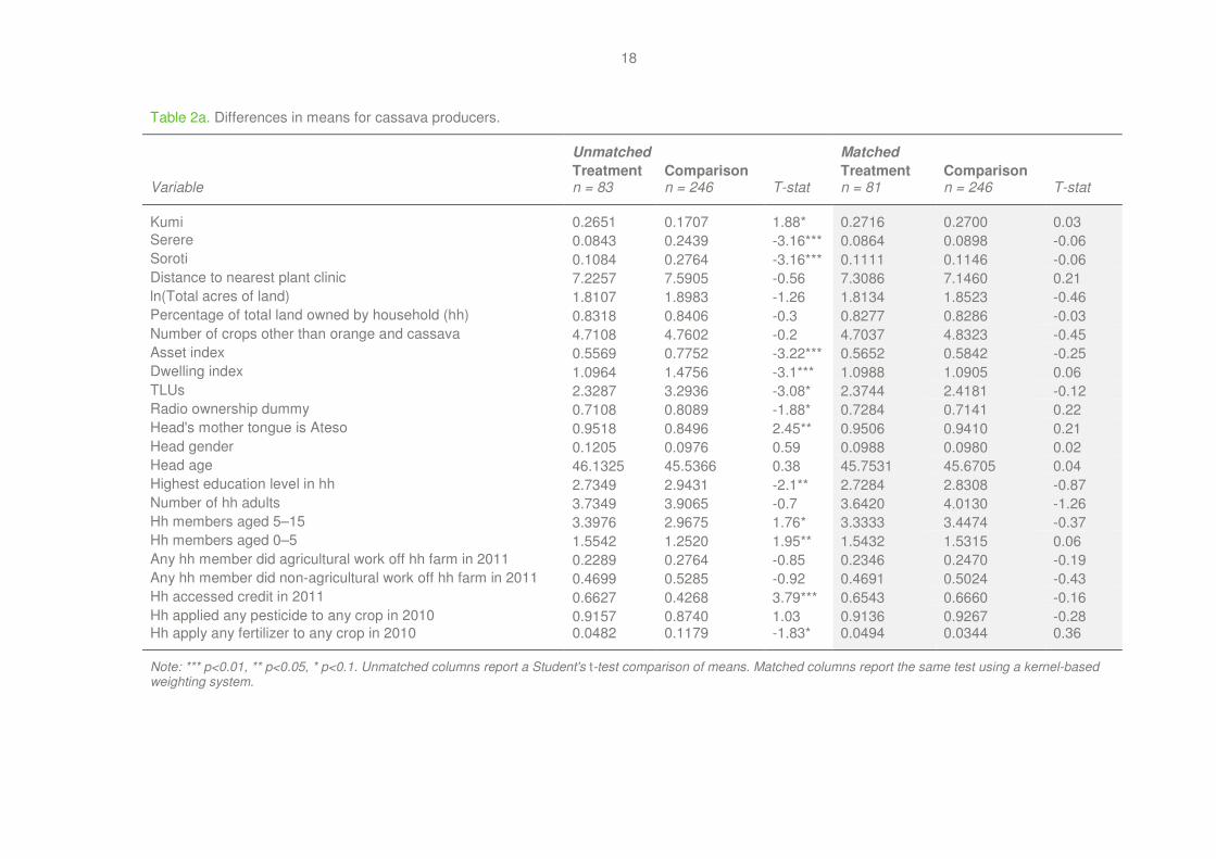
3.6 Cassava producer characteristics

This analysis considers 329 cassava producers, of which 83 were treated and 246 were comparison. Table 2a presents difference in means tests of household characteristics for cassava producers. The two tests presented and the variables considered are the same as those used for orange producers. As before, if the sampling process had succeeded in finding a perfect counterfactual, we would expect to see no significant differences between the groups. Approximately one-third of the treated and half of the comparison cassava producers are also orange producers. Note that, as discussed above, the cassava data considered here are not expected to show any impact from plant clinic treatment. This is because the advice given for cassava producers was predominantly preventive in nature, and therefore could not have been applied to any great effect by the time the survey was administered. Tests of impact were run as a check and are reported on briefly in Section 5.2. It is expected that if there are no systematic differences between the groups, and the plant clinic recommendations could not have been applied, then testing for plant clinic impact should find very small magnitude results with no statistical significance.

Thirteen statistically significant differences were found between characteristics of the comparison and treatment groups of cassava producers using the unmatched Student’s t-test. The treated households were more likely to come from Kumi, speak Ateso as their mother tongue, and access credit in 2011. They were less likely to come from Serere or Soroti, own a radio, and apply fertilizer in 2010. They also had lower asset scores, lower quality dwellings, fewer TLUs of livestock, lower household education levels, and more children. The prevalence of orange producers in the sample may partially be driving the higher wealth indicators of the comparison group since orange producers may be more commercially oriented and wealthier than the population average. Using the propensity score matching method, the significance of all these differences drops out. The lack of any significant differences seen when comparing the treatment with the comparison group constructed using propensity score matching indicates that a reasonable comparison group was created through this matching method.

18

Table 2a. Differences in means for cassava producers.

Unmatched Matched


Kumi 0.2651 0.1707 1.88* 0.2716 0.2700 0.03

Serere 0.0843 0.2439 -3.16*** 0.0864 0.0898 -0.06

Soroti 0.1084 0.2764 -3.16*** 0.1111 0.1146 -0.06

Distance to nearest plant clinic 7.2257 7.5905 -0.56 7.3086 7.1460 0.21

ln(Total acres of land) 1.8107 1.8983 -1.26 1.8134 1.8523 -0.46

Percentage of total land owned by household (hh) 0.8318 0.8406 -0.3 0.8277 0.8286 -0.03

Number of crops other than orange and cassava 4.7108 4.7602 -0.2 4.7037 4.8323 -0.45

Asset index 0.5569 0.7752 -3.22*** 0.5652 0.5842 -0.25

Dwelling index 1.0964 1.4756 -3.1*** 1.0988 1.0905 0.06

TLUs 2.3287 3.2936 -3.08* 2.3744 2.4181 -0.12

Radio ownership dummy 0.7108 0.8089 -1.88* 0.7284 0.7141 0.22

Head's mother tongue is Ateso 0.9518 0.8496 2.45** 0.9506 0.9410 0.21

Head gender 0.1205 0.0976 0.59 0.0988 0.0980 0.02

Head age 46.1325 45.5366 0.38 45.7531 45.6705 0.04

Highest education level in hh 2.7349 2.9431 -2.1** 2.7284 2.8308 -0.87

Number of hh adults 3.7349 3.9065 -0.7 3.6420 4.0130 -1.26

Hh members aged 5–15 3.3976 2.9675 1.76* 3.3333 3.4474 -0.37

Hh members aged 0–5 1.5542 1.2520 1.95** 1.5432 1.5315 0.06

Any hh member did agricultural work off hh farm in 2011 0.2289 0.2764 -0.85 0.2346 0.2470 -0.19

Any hh member did non-agricultural work off hh farm in 2011 0.4699 0.5285 -0.92 0.4691 0.5024 -0.43

Hh accessed credit in 2011 0.6627 0.4268 3.79*** 0.6543 0.6660 -0.16

Hh applied any pesticide to any crop in 2010 0.9157 0.8740 1.03 0.9136 0.9267 -0.28 Hh apply any fertilizer to any crop in 2010 0.0482 0.1179 -1.83* 0.0494 0.0344 0.36

Note: *** p<0.01, ** p<0.05, * p<0.1. Unmatched columns report a Student's t-test comparison of means. Matched columns report the same test using a kernel-based weighting system.

19

Table 2b. Cassava producer problems experienced.

Unmatched Matched


Brown streak disease 0.3253 0.2276 1.77* 0.3333 0.2687 0.93

Mosaic disease 0.2530 0.1585 1.93* 0.2469 0.2523 -0.09

Mealybug 0.0482 0.0366 0.47 0.0494 0.0399 0.3

Green mite 0 0.0122 -1.01 0 0.0191 -1.64*

Whitefly 0.1084 0.0407 2.3** 0.1111 0.0544 1.39

Aphids 0.2048 0.0935 2.71*** 0.1975 0.1392 1.07 Number of problems 0.9398 0.5691 2.87*** 0.9383 0.7736 1.02

Note: *** p<0.01, ** p<0.05, * p<0.1. Unmatched columns report a Student's t-test comparison of means. Matched columns report the same test using a kernel-based propensity score matching test

20

A comparison was made between the pest and disease problems experienced by treated and comparison groups of cassava producers. The results of this comparison are reported in Table 2b. The same slight difference in the survey question that was noted for orange plant problems was present for cassava problems. As above, however, the treated cassava producers preferred to discuss their current plant problems, which made the responses reasonably comparable. Cassava diseases reported include brown streak and mosaic diseases. Pests reported include mealybug, green mite, whitefly and aphids

8. T-tests

were run on the differences in mean disease prevalence between the treated and comparison groups. Treated cassava producers had significantly more instances of brown streak disease, mosaic disease, whitefly infestation, and aphid infestation. Treated households also reported 65% more problems with their cassava, and this difference was statistically significant. When differences in problem prevalence rates were compared between treatment and the comparison group formed using propensity score matching, all of these differences became insignificant. However, differences in green mite between treatment and control became statistically significant. Only two households reported experiencing green mite, and both were comparison households, so green mite was excluded from further analysis. A probit was run on the probability of attending plant clinics, controlling for the list of problems experienced and the full set of independent variables outlined above. In spite of the treated households’ generally higher problem prevalence rates, none of the problems had a significant impact on the probability of attending plant clinics when controlling for other factors. The lack of any statistical significance gives confidence that the problems experienced by treated producers did not systematically affect the decision to attend a plant clinic. However, the significance and magnitude of the differences between the groups using the unmatched comparison does raise concerns for the impact evaluation. Given that the treated producers appear to be experiencing greater plant problem prevalence, the yield and revenue results will be biased downwards, and labour and seedling expenditures might be biased upwards. However, given the nature of cassava, which is a relatively low maintenance crop, it is possible that the lower plant problem rates reported by the comparison producers are attributable to the group paying less attention to their cassava crops. If this is true, and the treated group is simply reporting more problems because they are paying closer attention to their cassava, then they might also be taking better care of their cassava, which might bias yield and revenue results higher.

3.7 Expected impacts of plant clinic attendance

Prior to this study, there was little direct evidence on what the impacts of the plant clinics would be for treated households, although there is a wealth of general information on agricultural extension activities in the literature. The expectation was that plant clinics were focusing on producers with plant problems. The specific advice given would vary by plant problem and pre-treatment producer practices, but was expected to include preventative and curative recommendations.

The preventive advice was expected to include selecting appropriate disease-resistant crop varieties, sourcing clean planting material, adding additional inputs (e.g. fertilizer) and changing labour practices (e.g. mulching, removing infected plants/fruits) in order to mitigate future disease pressure. In the short run, this type of advice was expected to increase the cost of planting material and fertilizer, and also to increase labour costs to apply new inputs and maintain plant hygiene. In the longer run, perhaps within three to five years, selecting disease-resistant plant varieties and employing methods to improve plant vitality and disease resistance is expected to increase yields. Following better preventive practices was also expected to lead to cleaner/higher quality produce, which could be sold for a higher price, and it was expected that the combination of higher and/or better yields and higher prices would lead to higher revenue.

The curative advice was expected to include adding or modifying use of chemicals (e.g. insecticides, fungicides) and labour practices (e.g. uprooting and destroying infected plants, removing infected fruits). Labour costs are expected to increase in the short run for producers who apply these types of recommendations. In cases where pesticide was needed the plant clinics were expected to prescribe appropriate products, application rates and handling practices. It was unclear whether applying this advice would cause a change in producer pesticide spending. Excessive pesticide use is a concern due to the dangerous nature of many of the chemicals used. The plant clinics were intended to follow integrated pest

8 The responses recorded in the survey for cassava problems were surprising. For example, aphids are not a significant

problem for cassava, although they can be serious for orange. In addition, the clinic plant problem records do not match the plant problems given by respondents in the dataset. It is not clear how these unexpected results occurred. This issue will be discussed in greater depth in Section 7.

21

management (IPM) principles of rational pesticide use and present options beyond a pesticide to control plant problems where appropriate, but did recommend pesticide use for producers where other options were not likely to succeed. Many orange producers routinely apply pesticide as a preventive measure, so it was possible that a plant clinic recommendation could simply have led to selection of a different pesticide without having an impact on cost. Curative advice was expected to mitigate short-term losses in yields, relative to producers with the same plant problems. The plant problems experienced by the treated and comparison groups for this study were not exactly comparable, as discussed in Sections 3.5 and 3.6.

Producers are assumed to be making rational decisions about production inputs based on their expected returns (Feder et al., 1985, p. 258). The plant clinics offer advice on how to best deal with problems the producer is experiencing, but offer no further incentive to follow the advice. This means they would not choose to adopt plant clinic recommendations if the expected benefits did not at least offset the costs. It was unclear ex ante to what degree plant clinic participation would alter producer practices, and whether the effects of curative or preventive recommendations would dominate. The lag time required to observe the full impact of plant clinic advice is not known, but it was expected that orange producers could have applied plant clinic advice and seen some impact on inputs and yields as a result of plant clinic attendance by the time of the survey. The time frame considered here is expected to capture only short-term impacts of the plant clinics. Labour costs and pesticide costs are predicted to rise as a result of producers applying curative advice. Yields are expected to rise due to plant clinic attendance compared to producers with exactly analogous plant disease and insect problems. If the treated producers were experiencing systematically worse plant problems during the study period, then curative advice would at best cause yields to be no different or slightly lower than for the comparison group. Applying preventive advice in the short run is expected to lead to increases in labour costs, planting material costs and fertilizer costs for the treatment group. If data were to be collected after a time period long enough for preventive advice to take full effect, then yields would be expected to show increases due to the application of preventive advice received from a plant clinic.

4. Methodology

This section presents the methods used to test for plant clinic impact. These were a household fixed effects difference in difference model; a propensity score matching with difference in difference model; and an inverse propensity weighted household fixed effects difference in difference model. Multiple tests were conducted to increase confidence that results obtained using any one test are not simply due to the self-selection bias inherent in evaluating this programme. All models incorporate difference in difference methodology, which controls for population-level changes across time and for the possibility that any unobserved time-invariant differences between treated and comparison producers could have influenced outcomes. Each test is run twice, once on the outcome of interest, and once on the de-meaned outcome of interest. The fixed effects difference in difference model is the preferred one for this analysis since it uses strict controls for individual differences, and is therefore unlikely to overstate programme impact due to unobserved differences between treated and comparison producers.

4.1 Difference in difference

The difference in difference method is widely used in impact evaluations because it can control for time invariant observed and unobserved differences between the comparison and treated groups that may affect the outcome of interest (Winters et al., 2010; Gertler et al., 2011). This is useful since if producers did have particular characteristics or practices that affected impact and that were not distributed identically between the treated and comparison groups, these might appear to be impacts of the plant clinics. Unfortunately, the difference in difference methodology cannot differentiate an unobserved variable that does change systematically across time for one group and not another from a plant clinic impact. A generic model of a household fixed effect difference in difference test is specified in Equation 6 below. �6�3 � ß� ( ß�D+*� ( ß,�D+*� ∗ D.��*�� ( E� ( F

Where: Y is the outcome variable αi is the time invariant effect on Y due to being in producer household i

22

Outcome variables considered are those described in Section 3.4 above. Time in this specification is a binary variable that is equal to one in 2011 and zero in 2010, so that ß1 will capture the (average) change in the outcome of interest that happened for the entire sample population across time. The value of ß2 captures the additional effect (if any) on the outcome resulting from being treated and allowing a year to pass. The error term µ contains all variation in Y not explained by the model. In a random effects difference in difference specification, a treatment binary is included to control for the possibility that some initial difference between the two groups affected the outcome of interest. With the standard model, control variables can be included to control for observable factors presumed to influence outcomes of interest. The household fixed effect model goes further than that by also controlling for unobserved time-invariant variation between treatment and comparison households that could affect outcomes of interest. Controlling for changes in the outcome variable due to other time invariant factors like treatment status is redundant and is therefore not included in the fixed effects specification. Although this is a fairly restrictive method to control for differences between the treated and comparison group, it still suffers from the limitation mentioned earlier: if there were time-variant unobserved variables that affected outcomes and changed systematically differently for the treated group and not the comparison group, the test cannot distinguish the changes from plant clinic impacts.

Since the data are set up as a panel using the producers’ recall information as baseline data, it is necessary to correct standard errors for the possibility of autocorrelation between observations coming from the same household at different points in time. If this is not done then the estimation might overstate the significance of the programme impact. This possibility is corrected for in each of the following estimates. Standard errors also account for the clustered sampling strategy, which leads to the possibility that outcomes could be clustered based on which plant clinic the producer was nearest to. Bootstrapped standard errors are used for both the fixed effect and the propensity score matching methods to adjust for the possibility that standard errors are not normally distributed.

4.2 Propensity score matching with difference in difference

Propensity score matching is a commonly used quasi-experimental method to construct a comparison group with which to estimate the impact of a treatment where treatment assignment was non-random (Caleindo and Kopeinig, 2008). Propensity score matching relies on matching treatment and comparison households on their observed characteristics in order to focus the analysis on households that are as similar as possible to the treated households. The first step in the propensity score matching process is to use probit regressions to estimate the probability for a producer to have been treated based on a set of observed characteristics that the plant clinics should have had no effect on. Results of this test for orange and cassava are reported in Tables 3 and 4 respectively. The model is specified in Equation 7. �7�Pr�D.��*�� 1|K� � L�KMß� Where: X is a vector of observed household characteristics ϕ represents the cumulative distribution function

The results of the probit regressions were used to estimate a number between zero and one for each producer. This number is the household’s predicted probability of receiving treatment and is known as its propensity score. This method assumes that the producer’s characteristics can be used to determine the decision of producers to attend a plant clinic. If the process worked, households with a similar propensity score should have similar characteristics. If there are households in treatment or comparison groups with no reasonable matches in the opposite group, these households are said to be off common support and are excluded from the analysis entirely.

The next step is to test whether the balancing property is satisfied; that is, the expectation that households with similar propensity scores have similar characteristics. The method used is to compare households to each other, weighting more similar propensity scores more highly. If the treatment and comparison groups are seen to have significantly different characteristics when the propensity score weighted method is used, then matching based on the propensity score process will not give a reliable estimate of impact. Tables 1 and 2 above showed that all differences between the treated and comparison groups became insignificant for both crops when comparing matched producers. Next, treatment and comparison were broken into four smaller blocks based on their propensity scores and a t-test was run for each independent variable in each block. No significant differences exist, so the balancing property is said to be satisfied for both crops. This process provides further assurance that households with significantly different characteristics do not receive similar propensity scores.

23

Once it is clear that the balancing property is satisfied and propensity scores do assign similar values to households with similar characteristics, it is possible to conduct propensity score matching tests for programme impact. The common support condition must be imposed a second time to further narrow the sample to households that form the best available comparison group. Imposing common support two times excluded two cassava treatments, and two orange treatments. This relatively low number of excluded households is not surprising given that the comparison households were selected to have similar characteristics to the majority of treated households.

The dependent variables for the propensity score matching impact tests are the difference in outcome between 2011 and 2010. The impact being estimated is therefore the difference between treated and comparison producers in the changes experienced over time, as seen in Equation 8. Taking this step means that any baseline differences between treatment and comparison households are removed, leaving only the change over time (Smith and Todd, 2005). Comparing the difference in mean of this new variable for the two groups is therefore similar to the ß2 coefficient on the time * treatment variable used to measure impact in the fixed effects difference in difference method outlined above. This means that time-invariant unobserved differences in the dependent variables are differenced out of the test. Conditioning the comparison on the propensity scores controls for any biases that would be introduced by observable characteristics (Imbens, 2004). �8�Y � ∆3�1� ∆3�0� � Q3�1�,�� 3�1�,��R Q3�0�,�� 3�0�,��R The propensity score matching uses a kernel-weighting scheme with replacement that draws on Heckman et al. (1997, 1998a, 1998b). Equation 9 describes the weight given to comparison producer j when comparing to treated producer i, which is based on the proximity of j’s propensity score to i’s propensity score. The closer the score relative to the average proximity of all comparison producers within the caliper width, the higher weight it receives. The propensity score matching specification is given in Equation 10. A caliper width of 0.1 is used, which means that each treated household value is matched with every comparison household whose propensity score is within ± 0.1 from that of the treated household in question. The outcome of interest of the comparison producers selected is multiplied by their kernel weight and the weighted average of these comparison households is taken as the best available matched outcome value for the treated household in question. The results from this analysis will be the average difference between the treated and comparison households’ outcomes when comparing with the best available counterfactual groups.

�9�T�+, �� U VW W�X Y∑ U �W� W�X ��∈�

�10��DD � 1��\∆3� �∆3 ∗ T�+, ��∈�

]�∈�

Where: Pi is the propensity score of producer i i ∈ treatment producers j ∈ comparison producers, such that (Pi – 0.1) ≥ Pj ≥ (Pi + 0.1) k ∈ comparison producers, such that (Pi – 0.1) ≥ Pk ≥ (Pi + 0.1) an is a bandwidth parameter N is the number of treatment producers

The benefit of the kernel weighting method as compared to the nearest neighbour(s) method is that it uses more of the available sample. This effectively magnifies the size of the comparison group. It is not possible to use bootstrapped standard errors with propensity score matching tests that use nearest-neighbour matching with replacement because the resulting matching estimator is not smooth (Abadie and Imbens, 2008). However, kernel based matching uses a greater number of comparison households for each treated household, which is expected to smooth the resulting estimator. This means it is reasonable to use bootstrapped standard errors for matching in order to ensure that any impact found is not observed in error (Abadie and Imbens, 2008, pp. 15-16). All standard errors also correct for errors clustered geographically around each plant clinic.

24

Table 3. Orange producer probability of attending a plant clinic.

Variable Coefficient p-value dy/dx p-value

Kumi 0.8452** (.017) 0.2864** (.012)

Serere 0.2343 (.556) 0.0794 (.555)

Soroti 0.6619* (.079) 0.2243* (.073)

Distance to nearest plant clinic -0.012 (.679) -0.0041 (.679)

ln(Total acres of land) -0.088 (.689) -0.0298 (.689)

Percentage of total land owned by household (hh) 0.1237 (.827) 0.0419 (.827)

Number of crops other than orange and cassava 0.0542 (.358) 0.0184 (.355)

Asset index 0.1761 (.403) 0.0597 (.403)

Dwelling index -0.052 (.654) -0.0176 (.654)

TLUs 0.0142 (.763) 0.0048 (.762)

Radio ownership dummy -0.4254 (.180) -0.1442 (.174)

Head's mother tongue is Ateso 1.4228*** (.001) 0.4822*** (.000)

Head gender -0.1923 (.648) -0.0652 (.649)

Head age 0.0026 (.793) 0.0009 (.793)

Highest education level in hh -0.1356 (.368) -0.0459 (.364)

Number of hh adults 0.0446 (.474) 0.0151 (.472)

Hh members aged 5–15 0.0876 (.139) 0.0297 (.132)

Hh members aged 0–5 0.149 (.129) 0.0505 (.120)

Any hh member did agricultural work off hh farm in 2011 -0.4996* (.068) -0.1693* (.062)

Any hh member did non-ag work off the hh farm in 2011 -0.2997 (.182) -0.1016 (.177)

Hh accessed credit in 2011 0.0015 (.995) 0.0005 (.995)

Hh applied any pesticide to any crop in 2010 -0.2038 (.731) -0.0691 (.731)

Hh apply any fertilizer to any crop in 2010 0.1628 (.553) 0.0552 (.552) Observations 188

Note: Values in parentheses are p-values. *** p<0.01, ** p<0.05, * p<0.1. Table reports a maximum likelihood estimation on probability to receive treatment.

25

Table 4. Cassava producer probability of attending a plant clinic.

Variable Coefficient p-value dy/dx

p-value

Kumi -0.4046 (.130) -0.1005 (.124)

Serere -1.6990*** (.000)

-0.4222*** (.000)

Soroti -1.1321*** (.000)

-0.2814*** (.000)

Distance to nearest plant clinic 0.0625** (.024) 0.0155** (.020)

ln(Total acres of land) -0.023 (.910) -0.0057 (.910)

Percentage of total land owned by household (hh) 1.0599*** (.009) 0.2634*** (.008)

Number of crops other than orange and cassava 0.1022* (.051) 0.0254** (.050)

Asset index -0.3578 (.176) -0.0889 (.172)

Dwelling index -0.1346 (.193) -0.0334 (.195)

TLUs -0.0514 (.288) -0.0128 (.285)

Radio ownership dummy -0.1146 (.620) -0.0285 (.620)

Head's mother tongue is Ateso 0.1527 (.693) 0.0379 (.693)

Head gender 0 (1.000) 0 (1.000)

Head age 0.0104 (.152) 0.0026 (.148)

Highest education level in hh -0.2002 (.116) -0.0498 (.116)

Number of hh adults -0.0037 (.947) -0.0009 (.947)

Hh members aged 5–15 0.0624 (.211) 0.0155 (.206)

Hh members aged 0–5 0.1011 (.157) 0.0251 (.152)

Any hh member did agricultural work off hh farm in 2011 -0.3552 (.119) -0.0883 (.116) Any hh member did non-agricultural work off hh farm in 2011 0.0573 (.752) 0.0143 (.753)

Hh accessed credit in 2011 0.4369** (.022) 0.1086** (.018)

Hh applied any pesticide to any crop in 2010 0.0655 (.814) 0.0163 (.814)

Hh apply any fertilizer to any crop in 2010 -0.7699*** (.008)

-0.1914*** (.008)

Observations 329

Note: Values in parentheses are p-values. *** p<0.01, ** p<0.05, * p<0.1. Table reports a maximum likelihood estimation on probability to receive treatment.

26

4.3 Inverse propensity weighting

In addition to the fixed effect difference in difference and propensity score matching with difference in difference methods outlined above, a fixed effect difference in difference with inverse propensity weighting method was also used. For this method, standard errors were calculated to correct for correlation between groups centred geographically around each of the plant clinics. The weighting system used is described in Equation 9 below, following on Asfaw et al. (2012).

�9�%� � ^1+_�.��*�� 1W� �1 W��⁄ +_�.��*�� 0

Where: wi is the weight assigned to household i Pi is the propensity score of household i

Weighting the comparison households by the inverse of their propensity score effectively gives households with higher propensity scores greater weight. The weights were applied to the household fixed effects difference in difference model outlined above. The results from this method are therefore based on a more closely matched group of observations. The same common support sample restriction in force for the propensity score matching is also used for the inverse propensity weighting to ensure that producers who are not reasonably comparable to the main sample do not affect the results. The inverse propensity weighting method incorporates propensity score matching and fixed effects regression techniques, which makes the results ‘doubly robust’, meaning the results will be reliable if either specification is correct (Imbens, 2004, p. 19).

5. Results

This section presents the results of the tests of impact. Orange producer results are considered in Section 5.1 and cassava findings are discussed in Section 5.2.

5.1 Orange producers

Table 5 presents results of the tests for impact for orange producers. Results for orange producer households suggest that the plant clinic programme did not achieve its goals of increasing producer output and profitability during the period between treatment and data collection. The fixed effect difference in difference test on fruit yield finds a coefficient of -584 kg/acre, and a coefficient of -.072 standard deviations from the mean revenue per acre for plant clinic users. Both of these findings are significant at the 90% confidence level. The propensity score matching and inverse propensity weighting tests also find declines in fruit yield, of a greater magnitude than that found by the fixed effect test. The propensity score matching findings are nearly significant at the 90% confidence level, and the inverse propensity weighting results are significant at the 95% confidence level. The results on the revenue tests were also negative, with roughly similar magnitudes to those seen for yield. All except one of the inverse propensity weighting revenue results were insignificant at conventional levels, suggesting that the revenue impacts were less clear than the yield results, but still consistently negative.

It is worth remembering that the time lag for plant clinic recommendations to translate into benefits to producers may often be greater than one year. Producers may take a few seasons to fully implement the recommendation, and the fully implemented recommendations may take a few seasons to have the full impact on yield and revenue. In this case, collecting data in the future for these same producers could reveal increases in producer output and profitability attributable to the plant clinics. It is also possible for treated producers to have had systematically worse disease problems than comparison producers. In this case, regression estimates would have significantly underestimated programme impact due to omitted variable bias. Given the care taken to sample comparison producers with similar macro disease risk factors such as climate and soil type, it is possible that simply collecting a follow-up round of data would mean that more comparison producers would experience similar plant problems, making the counterfactual case a more reliable comparison.

27

Table 5. Impact of plant clinic attendance on orange producers.

Variable DD FE DM DD FE DD PSM DM DD PSM DD IPW DM DD IPW

Cost

Pesticide -0.0177 0.0031 -0.0285 -0.1125 -0.0333 0.0001

(.646) (.132) (.372) (.397) (.365) (.972)

Fertilizer -1.4897 -0.0639 -0.8269 -0.036 -0.6628 -0.0095

(.656) (.741) (.817) (.789) (.851) (.960)

Seedlings -57.9956 -0.1566 -24.3554 -0.0551 -57.5874 -0.1376

(.340) (.345) (.685) (.647) (.235) (.377)

Labour 0.5682 0.0139 47.1226 0.0875 81.4781 0.0961

(.994) (.760) (.469) (.531) (.127) (.107)

Yield

Fruit -584.2257* -0.0717* -747.074 -0.2897 -1,143.8238** -0.1321***

(.087) (.091) (.114) (.137) (.014) (.008)

Seedlings 7.9778 -0.0633 17.8974 0.0664 17.4464 -0.03

(.820) (.733) (.600) (.614) (.665) (.897)

Aggregate

Cost -58.9348 -0.0678 21.9118 0.0296 23.1946 -0.0097

(.595) (.348) (.836) (.829) (.601) (.857)

Revenue -137.1208 -0.0294 -336.5727 -0.2123 -602.3788* -0.2571

(.448) (.755) (.190) (.141) (.065) (.130)

Profit 10.9017 0.0296 -306.7648 -0.1458 -542.3855* -0.2808

(.971) (.854) (.333) (.295) (.075) (.124)

Note: All variables are calculated per acre cultivated. Where the variable is monetary, the value is in terms of 2011 USD PPP. Values in parentheses are p-values. *** p<0.01, ** p<0.05, * p<0.10. DD = difference in difference; DM = de-meaned variable; FE = producer fixed effect; IPW = inverse propensity weighting; PSM = propensity score matching.

28

5.1.1 Orange production costs

None of the tests for costs returned statistically significant results. Fertilizer and seedling cost per acre all showed consistent declines due to programme participation. Despite the lack of significance, the consistent decreases of noteworthy magnitude found across multiple methodologies for seedlings suggest that the results observed may be true programme impacts which are simply too small to be captured with the available sample size. This suggests that treated households decreased their fertilizer use and seedling use relative to the comparison group as a result of receiving treatment. The lack of change in pesticide cost is somewhat surprising, given that many of the plant clinic recommendations included use of pesticide. It is possible that either the change happening in pesticide use has more to do with changing practices for pesticide application (e.g. application timing, selection of appropriate chemicals) rather than increasing expenditures, or that treated producers are simply not changing their practices. One of the goals of the plant clinics was to discourage indiscriminate or excessive use of pesticide, so the lack of change in pesticide cost is in fact an encouraging result, although it should also be noted that there is no other evidence showing that the plant doctors consistently and consciously gave advice according to IPM guidelines. The insignificant but consistent declines in fertilizer and seedling costs per acre are less encouraging results, since greater investment in either of these input types is expected to cause increases in farmers’ yields (Kraybill et al., 2012). However, as demonstrated by Duflo et al. (2008) in Busia, Kenya, perceived variance in returns to fertilizer use can cause farmers not to apply it, especially if it must be purchased at full market price. The lack of significant changes in fertilizer and seedling cost is not very surprising, as the plant clinics did not recommend either practice very frequently for orange producers or provide any incentive to do so. Labour cost rose across all tests, again with statistically insignificant results. The consistent findings suggest that the programme may have had some impact on labour, but any impact was too small to be captured with the available sample size. The impact found was larger using the two propensity score based methods, suggesting that comparisons using more carefully matched observations were better able to compensate for self-selection bias to estimate programme impact.

The total picture suggested by the orange cost per cultivated acre results is that the treated group was influenced to use a somewhat different selection of inputs. Treatment appears to have caused a preference for more labour expenditure, and less fertilizer and planting material expenditure. The lack of statistical significance for all of these results means that further inference must be made cautiously. The increase in labour expenditure of the treated group indicates that their crop problems were not causing them to simply give up on the crop. However, as noted above, many producers do not actually pay out of pocket for labour on their own farms. In cases where a producer is only using labour from within their household, the cost of using more labour on one’s own farm production is equivalent to the opportunity cost, or the next best thing the producer is foregoing in order to spend more time on their farm. In Teso, where options for off-farm employment are limited, the opportunity cost may be fairly small, meaning that producers might be more inclined to spend hours in labour than money on expensive inputs. The consistent decrease in other fertilizer and planting material expenditure does suggest that the farmers may have chosen not to make as much monetary investment in production in 2011, possibly due to higher infection/infestation levels than those experienced by the comparison group.

5.1.2 Orange yield

The results for the amount of orange fruit produced per acre were negative across all methodologies. The results from the fixed effects difference in difference and inverse propensity weighted difference-in-difference regressions were all statistically significant at or above the 90% confidence level. This means that treated producers had lower yields than the comparison group during the study period. This result contrasts with the generally positive (but highly variable) impacts on yields found for agricultural extension by Anderson (2007). The NAADS intervention in Uganda showed little or no impact on crop yields in the preliminary study by Benin et al. (2007). However, NAADS and the plant clinic intervention are not directly comparable. The decline in fruit yield found by the tests here is not a definitively negative result if treated households are seeking out treatment because they are experiencing problems beyond the normal level experienced. If this was the case, then the result suggests that the plant clinic intervention was not sufficient to completely mitigate the losses of the worse infected producers. This interpretation seems plausible since even in cases where the plant clinic advice was not ideal, following the advice still should not have led to losses in yields.

29

5.1.3 Orange aggregates

The results for the cost aggregate were indeterminate, with low statistical significance, suggesting that the changes observed in the components of cost described earlier roughly balance each other out such that the sum of all costs does not change. Aggregate revenue results were consistently negative, suggesting that the negative results observed in fruit yield translated to less money received for the farmers’ crop. The result for the de-meaned inverse propensity weighted difference in difference test is the only statistically significant revenue result. The consistently negative results for revenue across each methodology suggest that there were real differences. The lack of significance for most of the revenue tests can be seen as a positive result since the plant clinic users did have significantly lower yields, but this effect did not translate cleanly to lower revenue. The profit results were inconsistent and statistically insignificant except for the regular inverse propensity weighting results. This suggests that the negative results for revenue translated into declines in profit. The negative direction of the revenue and profit impacts is the opposite of the expected impact. The overall picture then suggests that the plant clinic intervention did not have the desired results for orange producers in the short term.

The orange results are all subject to the same uncertainty about potential differences in plant problems experienced by treated and comparison orange producers. The analysis in Section 3.5 showed that the treated producers did have a significantly higher likelihood of experiencing aphids, which might help to explain the reduction. The tests were re-run with the producers who experienced tristeza removed, and the results were not sensitive to their exclusion. In the longer term, it is likely that all households in the sample would experience similar problems given the similarities between the two groups and the similar geographical and climactic conditions. In the shorter term during which this analysis was conducted however, it is possible that the treated households had pest and disease problems that systematically worsened simultaneously with receiving treatment but not as a result of treatment; that is, an increase in actual plant problem intensity, which is separate from the potential increase in knowledge and reporting of plant problems, that could be attributed to attending the plant clinics. The difference in difference component of the tests used would account for any time invariant differences between the groups, meaning that any fixed characteristic including unobserved factors such as farmer aptitude does not impact on test results. It is also possible that treatment has a time lag greater than one year before it is effective in restoring or improving quantity produced. If the long-run effect of the programme is positive, then collecting another round of follow-up data would reasonably be expected to show more positive results.

5.2 Cassava producers

As noted above, the survey captured detailed data for cassava producers. The majority of cassava problems could only be addressed with preventive solutions (e.g. planting resistant varieties, following careful hygiene practices, using non-pesticide control measures) and therefore plant clinic advice would require at least a season to have impact. The quicker acting advice given to cassava farmers (e.g. apply insecticide, fungicide or soap solution) was largely not appropriate for the predominant cassava problems (viruses) and should not have caused any significant changes in output. The timing of the survey was such that planting advice could not have been implemented and should not be evident in the data. The same set of tests that were used for orange producers were run on cassava producers as a data check. Results of these tests are reported in Table 6. It was expected that these tests would show no results attributable to plant clinic attendance if the comparison group were statistically similar to the treatment group, since plant clinic advice could not have been implemented in the available time between receiving the advice and the survey collection.

The tests showed a consistent and significant increase in labour cost per acre, and suggested an increase in aggregate cost and revenue per acre. This indicates that there is some kind of a time variant unobserved difference between treated and comparison cassava producers, which the tests cannot distinguish from a treatment impact. One possible source of such a change was the data collection process itself, since it began with comparison households and moved to treated households, and may have changed systematically over time. The possibility exists that the severity of plant problems is changing systematically differently for treated producers than for comparison producers. This possibility was also present for orange, but the results moved in a substantially different way. Collecting a round of follow-up data would increase confidence in any results for cassava producers by providing data that depend less on farmer recall. It is possible that the reliance on recall data, particularly for a continuous crop like cassava, makes the data unreliable and therefore invalidates the robustness check. However, the results suggest that the cassava producer comparison group identified here may not be a reasonable counterfactual group for future analysis.

30

Table 6. Impact of plant clinic attendance on cassava producers.

Variable DD FE DM DD FE DD PSM DM DD PSM DD IPW DM DD IPW

Cost

Stem cuttings 5.5652 0.1305 -5.4645 -0.0789 2.2612 0.0659

(.392) (.379) (.541) (.512) (.668) (.505)

Labour 88.0136* 0.1816* 106.6763* 0.2955** 99.7546** 0.1965**

(.075) (.074) (.055) (.045) (.022) (.016)

Yield

Tubers 726.0479* 0.2632* -210.3717 -0.0653 -89.8154 0.0159

(.076) (.067) (.730) (.752) (.683) (.853)

Stem cuttings 31.0256 0.0775 51.3631 0.1192 68.7661** 0.1581**

(.634) (.542) (.519) (.549) (.039) (.040)

Aggregate

Cost 92.8555* 0.1861** 100.8763* 0.2741* 101.6921** 0.1960**

(.060) (.032) (.071) (.097) (.025) (.020)

Revenue 240.1514** 0.3343** -33.9636 -0.0444 25.9803 0.0967

(.021) (.017) (.839) (.811) (.625) (.349)

Profit 147.2958 0.0781 -134.8399 -0.1608 -75.7118 -0.099

(.193) (.529) (.419) (.364) (.352) (.367)

Note: All variables are calculated per acre cultivated. Where the variable is monetary, the value is in terms of 2011 USD PPP. Values in parentheses are p-values. *** p<0.01, ** p<0.05, * p<0.10. DD = difference in difference; DM = de-meaned variable; FE = producer fixed effect; IPW = inverse propensity weighting; PSM = propensity score matching.

31

5.3 Summary of impact findings

The tests considered here show that the plant clinics have not had the desired outcomes for orange producers in terms of yield and overall profitability during the time period of the study. The result is much less positive than the results found for other plant clinic programmes in Bolivia and Bangladesh (Harun-Ar-Rashid et al., 2010; Bentley et al., 2011). Both of these studies looked at changes over longer time periods, although it should also be noted that control groups were not included. The findings are less positive than much of the evidence on agricultural research and extension projects (Alston et al., 2000; Anderson, 2007). The shifts in input spending for orange producers are somewhat more promising, as they suggest no change in preference for pesticide use and a slightly greater preference for labour relative to the comparison group. If producers are spending more labour hours to control plant problems and not changing their pesticide practices, this is a positive result as it is generally consistent with an IPM framework for plant problem control practices (Morse and Buhler, 1997). It is possible that the changes suggested in input will cause yield and profitability to become more positive after more time has passed. However, the tests considered here present very little direct evidence that the plant clinics have succeeded at creating positive change in treated producer outcomes. Given this disappointing set of findings for orange producers, and work by Danielsen et al. (2012), which described some of the weaknesses in programme function, it is clear that the plant clinic programme needs refinement so that it can deliver on its goals. There are a number of possible factors beyond difficulties in plant clinic function that may be influencing the lack of impact found. These include: the short time being considered for producers to implement plant clinic recommendations; the relatively low statistical power of the study due to the combination of small sample size and large variance in the variables being considered; the reliance on recall data; and the potentially more severe plant problems being experienced by treated producers. The potential differences in plant problem severity for orange producers were discussed in Section 3.5, and the other concerns will be discussed in Section 7.

The results observed for cassava would be promising if it were reasonable to expect that plant clinic recommendations could have been applied by any of the treated households. Since it was expected that the treated cassava producers could not conceivably have applied the plant clinic advice by the time of the survey, the significance of the results found by the tests of impact are a concern, as they indicate some kind of bias in the data, which is affecting the treated and comparison households in systematically different ways. The possibilities include a difference in data collection due to surveying comparison producers first and treated producers afterwards, and systematically different plant problem prevalence between the two groups.

6. Programme function

The survey captured some new data about plant clinic function that have not been gathered in other monitoring efforts. This section summarizes that information, which will be of particular interest to the programme going forward. This section considers information provided by 413 households. Of these, 204 were plant clinic users and 209 were non-users. These are all the households who provided any information for any of the programme function questions. Not all of these households were considered in the impact evaluation due to lack of production data or being off common support. However, their information is still interesting for assessing programme function and input availability because these households participated in the economy that plant clinics operated in.

6.1 Plant clinic user characteristics

One question of interest for plant clinics is how treated producers became aware of plant clinic operation. Households were asked if they had heard of the plant clinics and if so, how. Those responses are captured in Fig. 2. The most common sources, in order of prevalence, were the banner at the plant clinic site, radio messaging and market people.

9 Several options that were expected to be significant ex ante were not

mentioned by any respondent, and are therefore excluded from the graph. The excluded sources were

9 Enumerators used ‘market people’ to capture a variety of different types of interactions. Generally all of these were

person-to-person interactions on a market day when the plant clinics were operating.

32

newspaper, pamphlet, household member and miking.10

Community meetings, church, community leaders and farmer groups also scored quite low, with fewer than five instances in each case. The ‘other’ responses primarily indicated some factor or factors at the market that led them to the plant clinic. The graph suggests that informal word-of-mouth interactions are the primary way in which households heard of the plant clinic. Radio announcements are also clearly an important method used by households to access information. The significance of radio as a method to hear about the operations of the plant clinics informed the inclusion of a radio ownership dummy as a control variable for the impact analysis. A little more than 75% of all households surveyed said they owned at least one radio, which adds to the evidence that radio messaging can be effective at making farmers aware of the plant clinics. As noted in key informant interviews, however, relying entirely on radio would not directly reach all producers, as some may not have a radio in their home and would therefore have limited access, and those that do have a radio may not necessarily listen to it.

Fig. 2. Sources where plant clinic users heard of the plant clinic.

For comparison households, the survey asked a series of questions about why they did not attend plant clinics. Those responses are summarized in Fig. 3. Sixty-five percent of respondents said they had not heard of the plant clinic. The responses given in the remaining 35% of surveys are summarized in the graph below. The predominant responses given were being too far from the plant clinic and being too busy to attend. The third most prevalent response was ‘other’, which was primarily producers indicating that although they had heard of the plant clinic they did not have enough information to prompt them to attend. The only other reason for not attending the plant clinic that was given more than five times was ‘not interested’. This, however, is not specific enough to offer much information to influence plant clinic design. The clearest takeaway from Fig. 3 is that non-user households who were aware of the plant clinic did not attend because it was not convenient for them. Given this was the case, then effort to expand plant clinic availability (e.g. more strategically placed locations, longer hours, more days of operation) should improve attendance. This need to expand plant clinic frequency and areas of operation was echoed in key informant interviews. Increasing the regularity of plant clinic operation would help to increase producers’ awareness and hopefully

10 Miking was employed by some of the plant clinics where a representative with a loudspeaker would broadcast

information about the plant clinics in an area where potential users congregated, e.g. a market.

42.86

4.596.12

1.53

48.98

.51

38.27

.512.04

7.65

010

20

30

40

50

Per

cent

of

resp

on

den

ts (

n =

196

)

Radio Extension worker Another farmer

Community meeting Banner Church

Market people Community leaders Farmer group

OtherNote: Respondents were asked to identify up to three sources. In total, 300 responses were given

33

their willingness to use the plant clinic. Danielsen et al. (2012, p. 47) showed the intermittent schedule of operations in six plant clinics in the region, three of which are considered in this paper. The irregularity of plant clinic operation is thought to be part of the reason why so many non-users were unaware of the plant clinics and so many plant clinic users attended a plant clinic spontaneously after seeing the banner or talking to other market people, rather than planning to attend it.

Fig. 3. Non-user producers who had heard of the plant clinics stated reason(s) for not attending.

The survey asked non-user households about what crop problems they experienced, which was analysed in Sections 3.5 and 3.6 above. Following that question, the non-user households were asked how they identified the problem that they experienced. The results of this query are presented graphically in Fig. 4. The respondents overwhelmingly said that they identified the problem they were having based on their past experience. The second most common source of information identified was family members or friends, with expert advice being a distant third. The overall results from this question suggest that it was rare for the non-user households to get external information about their crop problems. However, the results outlined in Fig. 5 suggest that the non-users did have a range of alternative plant problem information sources.

No analogous question was put to plant clinic users about how they identified their plant problem. The assumption underlying this un-asked question is that the plant clinics were the source of verification. Given the relatively large number of sources of plant information for plant clinic users and non-users outlined later in this section, it would be interesting to know what responses the plant clinic users would have given to a similar question. The omission is reasonable, however, since it was clear to the respondents that the plant clinics were the purpose of the survey they were responding to, and so the plant clinic users might well have given strategic answers to such a question.

8.47 8.47

3.39

23.73

38.98

5.08 5.08

1.69

13.56

6.78

16.95

010

20

30

40

Per

cen

t of

resp

onden

ts(n

= 5

9)

Knows how to handle problem Schedule conflict

Problem not important Too busy

Clinic too far away Inputs too expensive

Bad clinic reputation Don't think clinic can help

Not interested Got advice elsewhere

OtherNote: Respondents were asked to identify up to three sources. In total, 78 responses were given

34

Fig. 4. Non-users’ method(s) of verifying plant health problems.

The surveys asked farmers about other sources of information on plant problems to help shed light on the supply of advice in Teso. Both plant clinic users and non-users were asked if they received information on pests and diseases and, if so, what was the source of that advice, and did they use it? There were 378 producers that supplied sources for this question. The scope of the question is broad, but it does offer interesting data about what other information sources producers have access to. The results are presented graphically in Fig. 5 below. Radio is the most prevalent response, and NAADS comes in second. The two responses tell different stories. Radio is a delivery system, while NAADS is a national organization that delivers agricultural extension services and direct support to farmers. There is a possibility that the information the households heard on the radio was from NAADS or an NGO. The sub-county agricultural officers, lead farmers, household members, neighbours and farmer groups could also have been disseminating information from NAADS or an NGO.

Of those who checked ‘other’, a significant number of respondents listed newspapers as an external source of information. In about half of the newspaper instances, Etop

11 newspaper was mentioned specifically. This

suggests that newspaper coverage is an effective method of information sharing in Teso, even though it was not included as an option in the survey for this question. Plant clinics and personal experience were also commonly listed as ‘other’ sources of information. Curiously, newspapers were included as an option for the question analysed in Fig. 2 about how plant clinic users had heard of the plant clinics. None of the respondents mentioned it as a source for initial knowledge about the plant clinics. The lack of ‘newspaper’ responses recorded in the question illustrated by Fig. 2 and the presence of ‘newspaper’ in the ‘other’ category for the question responses shown in Fig. 5 together suggest that the plant clinics might make better use of newspapers to publicize their operations in the future.

11 Etop is a free monthly agricultural newspaper sponsored by Socadido, which is widely available in parts of Teso.

72.17

25.22

5.221.74

020

40

60

80

Perc

ent

of

resp

onden

ts(n

= 1

15)

Previous experience Family member/friend

An expert OtherNote: Respondents were asked to identify up to three sources. In total, 120 responses were given

35

Fig. 5. Sources of plant problem information other than plant clinics, by plant clinic user status.

Student’s t-tests were run on the prevalence of getting outside information from all of the specified options for the plant clinic users vs. non-users. Note that these groups are not the groups being considered in the impact analysis, but are considered here for the purpose of illuminating more general differences between producers who did and did not use the plant clinics. The results of these tests are presented in Table 7. Producers who attended the plant clinics were significantly more likely to get external information from neighbours, sub-county agricultural officers, NGOs, and ‘other’ sources. The plant clinic users listed a higher average number of sources, and they were more likely to seek information from every source. It is possible that these differences occurred if the plant clinic users had more severe problems that were also driving them to seek advice from more sources. For the programme going forward, it illustrates that the farmers coming to the plant clinics are also actively seeking out information from other sources. In order to expand the reach of the plant clinics, more effort will be required to reach additional households since the non-users may be less predisposed to seek information. Linking with other organizations and expanding the scope of information delivery methods is part of the larger Plantwise vision, of which the plant clinics are only part.

The Uganda Bureau of Statistics (UBoS) conducted a census of small- and medium-scale farmers from across Uganda in 2008/2009. Their survey asked a question similar to the one presented in Fig. 5 and Table 7. The questions are not exactly analogous between surveys, as the list of options UBoS presented differed from the list considered in this dataset, and in the UBoS survey households were asked to select only their primary source of plant problem information. Data from both sources are presented together in Table 8. Despite those differences, radio emerged as a prevalent source of information in both surveys as well as in key informant interviews. This reinforces the earlier conclusion that the plant clinics should continue to utilize radio as much as possible going forward.

One further question of interest was whether households with plant problems actually attended the plant clinics. The heart of this question is whether the producers with the worst problems are attending the plant clinics, which is necessary for the plant clinics to be able to fulfil the need for an advance warning system to agencies tasked with addressing national plant health issues. Getting a full answer to this question is beyond the scope of this dataset. The tests run on problems experienced in Sections 3.5 and 3.6 for the treated and comparison households did show that treated households reported greater likelihood to experience most problems, some of which were statistically significant differences. This would suggest that plant problem severity is positively correlated with plant clinic attendance. This is not conclusive, however, since the record

57.22

10.82

73.71

36.08

5.673.09

13.4

29.9

13.92

3.61

51.63

5.98

66.3

15.76

5.98

1.63

19.57

40.22

12.5

7.61

020

40

60

80

Per

cen

t o

f re

spo

nd

ents

by

use

r st

atu

sPlant clinic users (n = 194) Non-users (n = 184)

NAADS NGO Radio

Subcounty agriculturalofficer

Lead farmer Television

Household member Neighbour Farmer group

OtherRespondents were asked to identify all relevant sources. There were 480 separate reponses given by plant clinicusers, and 418 from non-users for a total of 898

36

of non-user plant problems relies on their own diagnoses, and it is plausible that comparison producers are diagnosing their problems less reliably than treated producers. It is also difficult to generalize since the sample was selected to capture comparison producers who were similar to those who attended plant clinics. If the plant clinics are seeing the worst plant problems, then the information from plant clinic records could be used to inform policy makers about the plant problem climate in Teso. However, the inference is weak, due to the problems listed and concerns about the quality of plant clinic records discussed further in Section 7. Further research is called for to evaluate how reliable the plant clinic information is as a diagnostic tool for the plant problems prevailing in their areas of operation.

Table 7. Percent of respondents using alternative information sources for plant problems.

Non-user Plant clinic user

Source n = 184 n = 194 p-value

Radio 66.3% 73.7% (.117)

NAADS 51.6% 57.2% (.277)

Neighbour 29.9% 40.2% (.036)**

Sub-county agricultural officer 15.8% 36.1% (.000)***

Household member 13.4% 19.6% (.106)

Farmer group 12.5% 13.9% (.685)

NGO 6.0% 10.8% (.091)*

Lead farmer 5.7% 6.0% (.899)

Television 1.6% 3.1% (.353)

Other 3.6% 7.6% (.090)*

Average number of sources 2.27 2.47 (.124)

Note: Table reports Student's t-tests, p-values in parentheses. *** indicates confidence at the 99% level, ** at the 95% level, * at the 90% level.

Another point of interest to the plant clinics that the survey can shed light on concerns the characteristics of the household member that actually attended the plant clinic. Table 9 provides some demographic information about these household members. In the dataset, there were no households where multiple household members attended the plant clinic. There was no reason that households could not have multiple members attend, but household practice seems to be to only have one member going to market and by default only one member attended the plant clinics. It is possible that multiple members attended, but the survey did not capture data for more than one attendee per producer household. In all but seven instances, the household member that responded to the survey was the same member who attended the plant clinic. The plant clinic users were 77.9% male and 82.8% were the household head. The average number of years of education was seven for all users. For female plant clinic users and non-head users, the average was five years of education. The 28 female non-head plant clinic users had an average of four years of education.

37

Table 8. Percent of households that received information on plant problems by source.

UBoS: primary source CABI: source(s) Source n = 3,046,419 n = 378

Radio 37.7% 70.1%

NAADS 7.7% 54.5%

Television 0.3% 2.4%

Other 1.1% 5.6%

Farmer to farmer 45.4%

Extension workers 5.4%

Agricultural shows 1.1%

Newspapers 0.6%

Magazines/bulletins 0.4%

Telephone 0.2%

Internet 0.0%

Neighbour 34.9%

Sub-county agricultural officer 26.2%

Household member 16.4%

Farmer group 13.2%

NGO 8.5% Lead farmer 5.8%

Note: UBoS (2010) survey allowed single answer, CABI survey allowed multiple answers. Grey shading indicates that the response was not directly comparable to responses in the other survey.

Table 9. Characteristics of the household member who attended a plant clinic (n = 204).

Male Female Age Non-head Head Total Non-head Head Total

20–29 2 17 19 2 2

30–39 3 39 42 11 3 14

40–49 43 43 5 4 9

50–59 1 31 32 8 3 11

60–69 1 16 17 1 6 7

70–79 6 6 1 1

80+ 1 1 Total 7 152 159 28 17 45

The gender imbalance among plant clinic users is a concern for the programme implementers going forward. It is likely that the gender mix of plant clinic users reflects the gender mix of household members who attend

38

the market from producer households. Key informant interviews confirmed that it was most often the male’s role to bargain in the market, which implies that the males were more frequently at the market. It is not acceptable to simply assume the maximum numbers of female producers are being reached without ensuring that every reasonable effort has been made to reach out to the female population. Gender inclusivity is of paramount importance, in order to ensure that larger development objectives are met. The programme implementers should therefore take care that the methods used to advertise the plant clinics are at least as effective at reaching women as they are at reaching men. Given that men are the primary market users for many households, it would be good to consider strategically holding plant clinics in alternative places at times when women do go outside of the household. It will also be important to continue to ensure that plant clinics are easy to use for women by having both female and male staff when possible.

6.2 Input availability

Another question of interest for the programme is whether farmers have access to the inputs that the plant doctors recommend using. Plant doctors are encouraged to interact with suppliers to ensure that the appropriate products they recommend to producers are available. The survey included questions aimed at finding whether producers had access to pesticide, fertilizer and planting material in 2011 and 2010. For each of these, this paper will address three questions.

1. How many plant clinic users and non-users reported having bought or used the input? 2. Which source(s) did the producers use to access the input? 3. For producers that did not buy the input, why not?

Enumerators recorded reasons that producers did not buy the specified input for some producers that had reported buying the input. This seeming contradiction was captured in cases where producers expressed reasons they were unable to purchase the full amount of the input that they believed was desirable. The graphs below present percentages of respondents who gave the specified input source or reason for not buying, by year and plant clinic user status. Because producers were able to give multiple responses to each question, the sum of the percentages is equal to or greater than 100% in each of the subgroups. Even though the limitations expressed were absolute for some producers (caused them to purchase none of the input) and relative for other producers (caused them to purchase less than their ideal quantity of the input), all responses are still included in the figures.

Data were also collected on whether producers had access to credit in 2011 and if so where. Credit is presumed to be beneficial to producers looking to invest in new crops, production techniques or products. It was unclear ex ante whether producers who attended plant clinics could access credit at all, so the question was included to get more data on credit access. This information is presented after the input availability analysis. Producers were also asked whether they experienced ‘major crop failure’ in either 2010 or 2011, and if so they were asked to identify the source. Plant diseases and infestations are only two possible sources of risk faced by producers attending the plant clinics. Information about other risk factors is of interest for the plant clinics going forward, and helps to broaden our understanding of the spectrum of problems faced by producers in this context. These data are analysed after the credit data.

The analysis also considers differences between the plant clinic user and non-user households. This section uses the same 209 non-users and 204 plant clinic users considered in Section 6.1, which are different from the comparison groups used for the impact evaluation. The comparisons presented here are about helping to understand characteristics of plant clinic users rather than trying to make estimates of impact or describe the quality of the counterfactual group. Table 10 presents Student’s t-tests on the differences in access to inputs between plant clinic users and non-users.

39

Table 10. Differences in input availability by plant clinic user status.

2010 2011

Plant clinic users

Non-users

Plant clinic users

Non-users

n = 204 n = 209 p-value n = 204 n = 209 p-value

Bought pesticide 92.2% 82.8% (.004)*** 91.2% 81.8% (.005)***

Applied pesticide 84.3% 70.3% (.001)*** 88.2% 73.2% (.000)***

Bought fertilizer 8.3% 10.5% (.447) 11.8% 12.9% (.722)

Applied fertilizer 5.4% 4.3% (.608) 7.4% 9.1% (.522)

Bought planting material

50.5% 37.8% (.009)*** 42.6% 47.5% (.312)

Accessed credit

57.8% 40.2% (.000)***

Experienced 'major crop failure'

76.0% 82.8% (.088)* 91.7% 90.0% (.548)

Note: Values in parentheses are p-values. *** p<0.01, ** p<0.05, * p<0.10.

6.2.1 Pesticide

The questions for pesticide and fertilizer were not crop specific, but were rather aimed at finding whether the producer had any access to the input or not. The number of positive responses for pesticide purchase and application remains fairly consistent from year to year. Table 10 includes some households that responded positively in only one year rather than both. Buying or applying pesticide in only one of the two years suggests that the producers’ purpose in the year they did buy/apply was curative rather than preventive. About 95% of the plant clinic users who bought pesticide reported doing so in both years, and about 91% who applied reported doing so in both years. For non-users, about 85% who bought and applied pesticide reported doing so in both years. The difference between the groups in likelihood to switch pesticide purchase and application practices from year to year is statistically significant. This difference suggests that more plant clinic users were using pesticide as a preventive measure relative to the non-user group.

Fig. 6 presents plant clinic users’ and non-users’ pesticide sources in both survey years. The distribution of sources was virtually identical in 2010 and 2011. By far the most common source given was the local market, with input dealers coming in second. These are normal commercial sources, and there is little evidence of non-commercial sources (e.g. NGOs, NAADS, others) involved in distributing pesticide. There were slight differences between the plant clinic users and non-users. Plant clinic users were significantly more likely than non-users to buy pesticide at the local market in both years. Non-users were more likely not to specify

12 their

source of pesticide in both years, with statistical significance in 2011. In 2010, no plant clinic users and only three non-users reported sourcing pesticide from an NGO.

12 Failure to specify is defined as responding affirmatively to purchasing the input in question, and then having no

response for the source where the input was purchased. This should not have been possible based on the structure of the questions in Section E4 of the survey (see Appendix 1), but still happened at a fairly high rate.

40

Fig. 6. Sources where producer bought pesticide by year and plant clinic user status.

Households were asked why they did not apply or under-applied pesticide, and these results are presented in Fig. 7. Producers were able to give reasons for not purchasing pesticide even if they had reported purchasing some in response to the previous question. These responses were captured when a producer was indicating why they did not purchase what they believed to be less than an optimal amount. When asked why they did not apply pesticide, producer responses varied somewhat from 2010 to 2011. More households reported having no pest problem as their reason to not purchase in 2010, while expense and non-availability became more prevalent in 2011. Specifying that the pesticides were not available or were too expensive indicates that the producers did actually make some type of inquiry. It is possible that some producers were having more serious plant problems in 2011, prompting them to make more inquiries about control options. After inquiring about problem control, they then ran into constraints due to pesticide cost or lack of availability in 2011 that they did not encounter in 2010. It is also possible that the difference is due to the fact that the 2010 data are subject to a longer recall period, which might cause producers to think about and describe the decision differently for the two years. The plant clinic users were significantly more likely to list excessive expense as the reason for not buying pesticide in 2011. None of the other changes were statistically significant.

For the pesticide question, ‘organic practices’ meant that the producer chose not to use pesticide, preferring instead to use ash or other non-chemical pest control strategies. This response is desirable from the point of view of the plant clinics if it indicates the use of alternative pest control strategies and if these strategies are effective at controlling the pests. Most of the plant problem control techniques other than pesticide involve significantly more labour and may be ineffective as a cure once a problem is out of hand. Alternative strategies also tend to have fewer negative externalities than pesticide use, particularly improper pesticide use. The increase in organic practices for plant clinic users is an encouraging trend, but it is not appropriate to attribute this change to the plant clinics. Many of the ‘other’ responses indicated that the households were either uncomfortable applying pesticide or lacked a sprayer or other appropriate equipment with which to apply it.

88.8

24.4

0 0 1.3

82.6

25.4

2.2 .7 1.4

86.5

25.8

0 .62.5

84.3

31.4

0 .7 .7

020

40

60

80

100

Plant Clinic User Non-User Plant Clinic User Non-User

2010 (n=298) 2011 (n=303)

Local market Input dealer NGO/project

NAADS OthersNote: Respondents were asked to identify all relevant sources. There were 352 total responses from 163 usersand 140 non-users in 2011, and 338 total responses from 163 users and 138 non-users in 2010

Per

cent

of

resp

ond

ents

41

Fig. 7. Reason(s) producer did not buy pesticide by year and plant clinic user status.

In summary, pesticide is fairly widely used by the producers sampled for this analysis. Most producers purchase their pesticide at market prices from marketplace vendors. These are the main sources that plant clinic doctors should be networking with to ensure that the products they recommend are available. However, cost is perceived as a larger barrier to producers purchasing optimum amounts of pesticide than availability.

6.2.2 Fertilizer

Fertilizer purchase and application were both reported as much less frequent than pesticide purchase and application. In total, 13% of non-users and 12% of plant clinic users reported buying fertilizer in 2011, compared with 11% of non-users and 8% of plant clinic users who bought fertilizer in 2010. Along with this, 9% of non-users and 7% of plant clinic users reported applying fertilizer in 2011, compared with 4% of non-users and 5% of users in 2010. None of the differences between the users and non-users were statistically significant. The question focused on mineral fertilizer rather than organic fertilizer. Organic fertilizer includes manure, mulching, and other relatively lower cost and more labour-intensive practices. Organic fertilizer is more commonly used than mineral fertilizer in eastern Uganda (2010). The responses captured here indicate that mineral fertilizer use is relatively uncommon, but should not be interpreted as general evidence that any fertilizer use is rare. The findings for fertilizer purchase in Table 10 are fairly consistent with the UBoS (2010) findings that showed approximately 10% of farmers in the eastern region applied ‘inorganic fertilizer’, but are slightly higher than the 5% of farmers applying mineral fertilizer reported by Benson et al. (2012). This relatively low use of fertilizer in general and mineral fertilizer in particular is a wider concern for Ugandan agriculture (Benson et al., 2012; Bayite-Kasule, 2009). Responses indicated that fertilizer was applied less often than it was purchased for both groups in both years. It is unclear why this should be the case since purchasing fertilizer implies spending money without any possibility of receiving a benefit if it is not applied. One possibility is that the producer simply had not yet applied the fertilizer purchased, although this seems unlikely for fertilizer purchased and not applied in 2010. Benson et al. (2012) found that most producers in Uganda used fertilizer within a week after purchase, but that a sizeable minority stored it for up to two months prior to application. It is possible that purchased fertilizer is being lost in storage, or sold/bartered on to other buyers, or simply given to other producers.

Fig. 8 presents producer responses to the question about where producers purchased fertilizer, by year and plant clinic user status. The sources of fertilizer varied noticeably between 2010 and 2011. The local market

25

55

10

0

15

29.5

45.5

18.2

2.3

22.7

8

64

16

4

20 20.5

40.9

13.6

9.1

29.5

020

40

60


2010 (n=42) 2011 (n=47)

No pest problem Too expensive Organic practices

Not available OthersNote: Producers were asked to identify all relevant reasons. There were 78 total responses from 25 users and22 non-users in 2011, and 73 total responses from 20 users and 22 non-users in 2010.

Per

cent

of

resp

ond

ents

42

and input dealer sources both increased in prevalence from 2010 to 2011. Plant clinic users had a significant increase in likelihood to buy from an input dealer from 2010 to 2011, and were significantly more likely than the non-users to do so in 2011. The plant clinic users had a significant drop in likelihood to not specify where they bought fertilizer from 2010 to 2011. One possible explanation for this finding is that the plant clinic users were making more careful fertilizer purchases in 2011 than in 2010 since they were better able to specify their sources, and were mentioning input dealers more frequently, which is likely to be a more reliable source for fertilizer. Another possible explanation is that the 2010 responses were dependent on a longer period of recall, which might cause producers to describe their reasons for not buying fertilizer differently. The government attempts to regulate the import of inorganic fertilizer, but there is little oversight for fertilizer retailers dealing directly with producers (Benson et al., 2012). The plant clinics were not necessarily completely omitting to recommend fertilizer, but the records kept at the plant clinics did not include fertilizer as a possible recommendation, which suggests that fertilizer recommendation was not emphasized strongly but also means there is no direct evidence to test that suggestion. Given the relatively low prevalence of mineral fertilizer in Uganda, it is likely that plant clinics will need to expend greater effort to encourage its use.

Fig. 8. Sources where producer bought fertilizer by year and plant clinic user status.

Fig. 9 shows reasons given for not buying fertilizer by year and plant clinic user status. Plant clinic users were significantly more likely to report lack of availability as a reason to not buy fertilizer in both years. However, lack of availability is low on the list of reasons given for not buying fertilizer, and the number of respondents reporting this reason declined slightly for both groups in 2011. Organic fertilizer prevalence as a reason for not buying mineral fertilizer remained fairly constant between the two years, and across both groups. Plant clinic users were less likely than non-users to give high cost as a reason they did not buy fertilizer in both years, with the difference being statistically significant in 2011.

30 30

20

0 0

20

40

6.7

33.3

13.3

0

13.3

21.1

47.4

15.8

5.3 5.3

15.8

47.6

14.3

23.8

4.8

0

23.8

010

20

30

40

50


2010 (n=25) 2011 (n=40)

Local market Input dealer Other dealer

NGO/project NAADS OtherNote: Producers were asked to identify all relevant sources. There were 45 total responses from 19 users and21 non-users in 2011, and 26 total responses from 10 users and 16 non-users in 2010.

Per

cent

of

resp

ond

ents

43

Fig. 9. Reasons producer did not buy fertilizer by year and plant clinic status.

6.2.3 Planting material

The survey asked if the farmer bought orange seedlings or cassava cuttings in 2010 and 2011. These two types of planting material are specific to orange and cassava, while the pesticide and fertilizer questions referred to any purchase for any crop.

13 The question about buying planting material was not followed up

with a question about whether the producer actually used the material. For cassava producers, it is normal to plant cassava cuttings yearly. It is also common to plant cuttings that were not bought but gathered from the previous year or borrowed from a neighbour. Orange seedlings are not necessarily planted yearly, as the trees live for longer periods of time and will bear fruit over multiple years. For both crops, buying planting materials is likely to represent an investment in new or improved varieties, as many farmers already have access to non-market sources of planting material with low or no cost. Plant clinic users were more likely than non-users to buy planting materials in both years, although the gap became smaller in 2011. In 2011, 48% of plant clinic users and 43% of non-users reported buying planting material, compared to 50% of users and 38% of non-users in 2010. The difference in 2010 was statistically significant at the 99% confidence level.

Fig. 10 presents producer responses regarding where they bought planting material by plant clinic user status and year. The responses were similar across 2010 and 2011. The most frequent response was ‘other farmers’. This was not one of the listed options in the survey form, but was frequently specified by farmers as an ‘other’ response. Plant clinic users were more likely to give this response, with the difference between users and non-users being significant in 2011. There were 12.7% of 2011 respondents and 16.4% of 2010 respondents who did report buying planting material but did not specify any source. The question did not differentiate between cassava and orange, but it is likely that the respondents citing ‘other farmers’ as a source were predominantly referring to cassava cuttings since borrowing or trading for cuttings is commonplace. Orange seedlings can also be sourced from other specialist farmers, but the practice is much

13 The questions for pesticide and fertilizer purchase asked which crop(s) the producer had used the input for. It included

check boxes for cassava and orange, and a check box for any other crop. See Section E4 of the survey in Appendix 1 for the exact question(s).

29.4

42.9

37.3

13.6

4.5

35.7

50.3

39.2

6.4 5.8

29.5

37.638.7

119.2

35.1

51.1

38.5

4.66.3

010

20

30

40

50


2010 (n=348) 2011 (n=347)

Fertility acceptable Too expensive Organic practices

Not available OtherNote: Producers were asked to identify all relevant reasons. There were 454 total responses from 173 users and174 non-users in 2011, and 461 total responses from 177 users and 171 non-users in 2010.

Per

cent

of

resp

ond

ents

44

more common for cassava. The question did not ask the producer to specify which crop they were purchasing the planting material for, meaning it was not possible to differentiate the answers to this question by crop. Overall, it appears that farmers are only rarely using planting material from NAADS or other more reliable sources. It is possible that the planting material sourced from other farmers would be of a desirable variety, but without further detail on the quality of the material accessed, this cannot be assessed.

Fig. 10. Sources where producer bought planting material by year and plant clinic user status.

Farmers that reported not buying or under-buying planting materials were asked what their reason was for not purchasing. Their responses are summarized in Fig. 11 by year and plant clinic user status. The responses largely suggest that households who did not buy planting material were still able to plant as much as they needed by using their own planting materials, or borrowing as necessary. These responses are consistent with traditional practices for cassava, although as above the question did not specify by crop. No producers cited lack of availability of planting materials as a reason for not buying. The plant clinic users were more likely to use their own planting material, with the difference being significant in 2010.

There was relatively little difference in the planting material buying practices of plant clinic users compared to non-users. The lack of difference is unexpected, given the importance of selecting appropriate varieties and sourcing clean planting material to combat viral diseases in both cassava and orange, and the apparent differences in the pesticide and fertilizer buying practices observed for the two groups. As noted, it is not possible to say definitely whether the planting material reported on was acquired for orange or cassava production. However, it is likely that the majority of the responses refer to cassava cuttings, as these are planted annually and in greater quantities than orange seedlings. Producers who reuse their own cassava cuttings run greater risk of perpetuating viral diseases common in cassava, so it would be reasonable to expect using one’s own cuttings to be correlated with more serious problems. Seeking out clean planting material is an important practice for dealing with virus problems in cassava. The plant clinics should be careful to recommend reputable sources for clean, disease-resistant planting material when available, as the plant clinic users seem to have kept relatively similar sources of planting material despite receiving advice.

31.3

12.5

0 0

5.2

77.1

8.3

35.6

6.8

0 0 0

69.9

1.4

36.5

7.1

0 0 0

81.2

4.7

26

6.8

1.4 1.4 1.4

69.9

5.5

020

40

60

80


2010 (n=158) 2011 (n=169)

Local market Input dealer Other dealer

NGO/project NAADS Other farmer

OtherNote: Respondents were asked to identify all relevant sources. There were 192 total responses from 85 usersand 73 non-users in 2011, and 212 total responses from 96 users and 73 non-users in 2010.

Per

cent

of

resp

onden

ts

45

Fig. 11. Reasons producer did not buy planting material by year and plant clinic user status.

6.2.4 Credit access

Respondents were asked whether they had used credit in 2011. The survey did not ask about credit use in 2010, so this section considers 2011 only. There were 118 plant clinic users that accessed credit in 2011, compared to 84 non-users. This difference was statistically significant. Securing credit access requires effort from the farmer, as does accessing plant clinics. As noted above, the plant clinic user and non-user groups considered here are different from the comparison and treated household groups considered in the impact evaluation portion of this analysis. However, the significant difference in credit access further supports the idea that the plant clinic users were in some way different to the non-users.

Fig. 12 shows the sources of credit that producers used in 2011. Not all producers specified where they received credit from, so these are not captured in Fig. 12. SACCO is a Savings and Credit Co-operative Organization, which is a government-run savings and credit programme aimed at small-scale producers and business persons like those in the survey. MFI is any other microcredit institution operating in the area not otherwise specified. VSLA is the Village Savings and Loan Association, which is a type of small, relatively informal lender organization at the village level. VSLAs were specified frequently by respondents so were included as a unique source. There were some significant differences in credit source between the plant clinic users and non-users. Plant clinic users were significantly more likely to access credit with a VSLA, and significantly less likely to use NGO or SACCO credit. The question in this survey was fairly permissive about possible sources of credit, and found about half of the respondents reported having used credit in 2011. This is a much higher rate than the 9.3% of producers reported to be accessing credit within the last five years in eastern Uganda by UBoS (2010). If households are credit constrained, it is possible that greater access to credit would lead to greater use of the other farm inputs. The survey did not ask why producers did choose to access credit, or why those who did not access credit did not do so, nor did it ask whether the producer had as much credit as desired.

84

4.3

0

11.7

4.3

77.5

7.2

0

21.6

7.2

86

20

14

0

78.6

8

0

23.2

.9

020

40

60

80


2010 (n=205) 2011 (n=212)

Used their own Too expensive Not available

Borrowed OthersNote: Respondents were asked to identify all relevant reasons. There were 212 total respondents from 100 users and112 non-users in 2011, and 205 total responses from 94 users and 111 non-users in 2010.

Per

cent

of

resp

ond

ents

46

Fig. 12. Credit source(s) in 2011 by plant clinic user status.

6.2.5 Major crop failure

Respondents were asked whether they had experienced ‘major crop failure’ in 2010 or 2011. The responses help to describe risk factors faced by producers in the context that the plant clinics operate. Almost all the producers surveyed reported experiencing major crop failure in both years, which raises questions about how this particular survey question was interpreted by producers. The question did not limit producers to cassava or orange failure. Given that almost all of the producers surveyed were growing multiple crops, it is possible that the problems specified damaged some but not all of the crops. The survey did not specify what ‘major crop failure’ meant, nor did it ask the farmer to quantify the severity of the loss they experienced.

Fig. 13 shows the sources of crop failure by year and plant clinic user status. Overall, the two groups show fairly similar reasons for crop failure. This suggests that the sampling strategy was broadly successful at finding a comparison group with similar risk factors. The most dramatic change in source of crop failure was excess water (e.g. rain and floods), which became significantly more prevalent for both groups from 2010 to 2011. This is unexpected, since there was some evidence of flooding in 2010, and not 2011. It may indicate that farmers were reporting the loss of production in 2011 that resulted from flood damage to young crops in 2010. Alternatively, non-users reported significantly lower prevalence of failure due to lack of water in 2011 than 2010. Pests and/or diseases became significantly more prevalent for plant clinic users from 2010 to 2011. The difference between users and non-users became statistically significant in 2011. The plant clinic users reported a significant decline in farm raids as a source of crop failure in 2011, and were also significantly less likely to report farm raids than the non-users in 2011. The plant clinic users were significantly more likely to report a household member falling sick as a reason for crop failure in 2010. Hailstones became significantly more prevalent as a source of crop failure for plant clinic users in 2011, as compared to plant clinic users in 2010.

2526.7

3.3 1.7

40

66.7

11.7 10.1

26.6

1.3

20.322.8

17.7

3.8

020

40

60

80

Plant Clinic Users (n=57) Non-Users (n=79)

Per

cent

of

resp

onden

ts

Bank SACCO MFI

NGO Family or friend VSLA

OtherNote: Respondents were asked to identify all relevant sources. There were 105 responses from users and81 from non-users.

47

Fig. 13. Reason(s) for ‘major crop failure’ by year and plant clinic user status (HH = household).

6.3 Plant clinic recommendations

This section will consider questions regarding how well the programme worked for treated households. The data used come from the household survey created for the impact evaluation, supplemented with data from plant clinic records for the treated households. First, the diagnoses and recommendations from the plant clinic records will be compared to the data from the survey. This comparison will describe how well producers’ recollection matches plant clinic records, which is of interest in assessing whether enough is being done to ensure that producers can apply the recommendations that are given. The section closes with analysis of whether producers do actually apply the recommendations.

6.3.1 Recommendation recall

Whether farmers remember the advice that was given can be addressed by comparing the plant clinic records with the household description of the advice captured in the survey. This is an interesting question since it will inform future plant clinic efforts. One question that it will not be able to address is the possibility that plant clinic records were entered incorrectly initially. This is a concern since client volume was high during the short window of plant clinic operation in some locations, and entering all the data necessary for the plant clinic records took a significant amount of plant doctors’ time. Due to this concern, it is unclear that either source can be taken as a definite description of the interaction at the plant clinic.

The problems farmers reported did not match up well with the problems recorded in the plant clinic record. Treated orange producers reported 232 total problems in the survey, while plant clinic records describe 161 problems. Of these problems, 75 were matched, which was 19.1% of the total problems noted. Treated cassava producers noted 150 problems, and plant clinic records mention 72 problems. Of these, 22 matched, which was 9.9% of the total number of problems. These rates of matching between the survey and the plant clinic records are much lower than recorded in assessments of plant clinics in Bolivia (Bentley et al., 2011) and Bangladesh (Harun-Ar-Rashid et al., 2010, p. 16). This low match rate suggests that there is a considerable communication gap between plant clinics and producer decision-making, but it is also possible and perhaps more likely that there were problems with the data collection process. One possible source of data collection error is the translation of plant problem names from Ateso or Kumam to English. Since there were no visual aids such as fresh samples or photos to verify the cause of the problem, the risk of error is

55

20

55

1115

0

88

20

3

21

61

19

55

1517

1

83

20

5

27

51

56

68

1918

1

83

1 0 1

21

4650

59

1922

1

80

20

3

25

020

40

60

80


2010 (n=388) 2011 (n=397)

Lack of water Excess water Pests or diseases

Hailstones Animals or theft Sickness

HH member sickness HH member lost job Civil unrest

Farm raid OtherNote: Respondents were asked to identify all relevant reasons. There were 1240 responses from 196 users and201 non-users in 2011, and 1072 total responses from 192 users and 196 non-users for 2010.

Per

cent

of

resp

on

den

ts

48

high, both due to memory decay or misdiagnosis by the farmer and to mistranslation by the enumerator. One conspicuous example of a mismatch is ‘aphids’ in cassava, which was recorded 21 times in the survey, translated from ‘eliana’ in Ateso. However, aphids are not a common pest in cassava and had not been recorded in the plant clinic records. Other potential error sources include poor communication during the initial plant clinic interaction, producers failing to recall correctly, producers giving current crop problems rather than the crop problems that were brought to the plant clinic, and errors in plant clinic record keeping. This analysis assumes that the plant clinic records are more reliable than producer recall captured in the survey.

Comparing recommendations given for the problems diagnosed yielded slightly better results, which suggests that households were somewhat better at remembering what to do than remembering the specific name of the problem. Treated orange producers reported 205 recommendations, compared to 177 from the plant clinic records. The lower number of recommendations than problems reported on the survey suggests that the respondents listed current problems rather than problems brought to the plant clinic, since the number of recommendations in the dataset should have met or exceeded the number of problems diagnosed. Of the interview and plant clinic record recommendations for orange producers, 109 matched, which constituted 28.5% of all recommendations. For cassava producers, 167 recommendations were listed in the surveys, and 84 in the plant clinic records. Of these, 31 matched, which constituted 12.4% of all recommendations. The match rates are slightly higher than for diagnoses. One possible explanation for this is that the translation issues are less challenging for tasks than for problem names. Another possibility is that producers may have clearer memory of the countermeasures they have taken than the specific name of the problem they were dealing with. The matching rate is still quite low for recommendations, however, which raises concerns similar to those raised for diagnoses above. There is a gap between the plant clinic records and the producers’ recollection of the plant clinic interaction. It is unclear whether the issue is with record keeping, the survey process, producer recall, or a true difference in understanding of the plant clinic interaction.

The disconnect between producers’ recollection and plant clinic records is an issue that needs to be addressed by plant clinics going forward. It is crucial that plant clinic diagnoses and recommendations are correct, and that information is communicated to the producers in such a way that they remember the advice correctly and are able to follow through on it correctly. Work by Danielsen et al. (2012, pp. 51–58, 2013) using records from some of the plant clinics considered here found some evidence of incomplete diagnoses

14 and recommendations

15 being given. They found that 47.6% of all cassava diagnoses were only

partially complete and rejected 17.7% as incorrect. For orange diagnoses, they found 58.0% only partially complete and rejected 38.4%. They moved on to assess the quality of the recommendations for the most prevalent diagnoses, including cassava brown streak disease and orange leaf miner. The cassava brown streak disease recommendations were judged to be 95.5% partially effective and 2.3% ineffective at controlling the diagnosed disease. Orange leaf miner recommendations were found to be 20.0% partially effective and 80.0% ineffective. This assessment is based on a larger set of ‘best practices’, which makes further inference difficult since plant doctors may have been editing the ‘best practice’ advice to a more feasible set of recommendations in some cases, and/or may have been omitting parts that the producer was already practicing. However, the large percentage of recommendations that are not ideal is troubling, as following ‘best practices’ is expected to be the most effective set of problem control measures.

14 The validation methodology of Danielsen et al. (2012, 2013) is based on five criteria: specificity, plausibility, likelihood,

consistency and ambiguity. A diagnosis was rejected if the diagnosed problem was not common for the crop and was not present in the geographic area, and the symptoms recorded did not match the general symptoms of that disease. Conversely, if these three criteria were met, but the diagnosis was not specific or did not uniquely identify a particular problem, the validation of the diagnosis was partial. The authors further say that ‘partial’ indicates there is some doubt about the diagnosis. If all criteria were met then the diagnosis was described as complete, indicating no doubt about its validity.

15 Danielsen et al. (2012) assessed recommendations given for five of the major diseases the plant clinics encountered,

which included cassava brown streak disease and orange leaf miner. They classified recommendations as either best practice, partially effective, or ineffective. Partially effective describes a recommendation that “will reduce spread and severity of the disease but only to a limited extent”. The definition of best practice to combat cassava brown streak disease was to uproot and destroy the infected plants, use disease-free planting material and disease-resistant varieties. Best practice against orange leaf miner was to remove and destroy the infected plant parts, prune the tree, and apply pesticide in the case of young trees.

49

The analysis presented here shows that there was a low likelihood of farmers actually remembering the information given in the way that the plant clinic recorded that it was communicated. It is important that plant clinics diagnose problems correctly, and the recommendations are sound. It is also important that plant clinic records be kept carefully so that the plant clinics can provide reliable data to other organizations about the plant problems faced by producers in order to fulfil the larger Plantwise vision. Future surveys need to be explicit in specifying that the problems of interest are the ones that were addressed by the plant clinic, and then including another question for plant clinic users to describe current plant problems. The finding also suggests that further effort should be made to ensure that farmers remember the recommendations given at the plant clinics. Providing a written record of the diagnosis and recommendations to producers would be a desirable step to directly address the difficulty of remembering the interaction. This practice is one of Plantwise standard operating procedures (Bentley et al., 2011) – but not always followed in earlier phases of the plant clinics. Improving record keeping at plant clinics and surveys’ capacity to gather the required information will allow future comparisons to be made with greater certainty that discrepancies (if any) are due to genuine communication or recall differences rather than data issues.

6.3.2 Recommendation uptake

Whether producers actually followed the recommendations of the plant clinics was addressed by considering two questions from the survey, as well as plant clinic records.

16 The information from plant clinic records was

not used for this comparison, however, since it was not clear that the plant doctors would have any comparable information on producers’ actual recommendation uptake. When producers were asked directly whether they followed one of the recommendations from the plant clinics, 81.5% of the responses received for orange recommendations were positive. Cassava producers said they followed the plant clinic recommendations in 48.8% of the responses. This relatively lower uptake rate for cassava producers does suggest that the claim made by this paper that it is premature to evaluate cassava producer outcomes is reasonable. Not all plant clinic users responded to this question for each recommendation, so the number of responses is lower than the expected maximum.

Producers were also asked what portion of their acreage planted with the relevant crop they followed the recommendation on. Some comparison households also answered this question, which shows that the answers given for this variable were subject to variation in enumerator interpretation. Of the 100 responses given by treated orange producers, 74 indicated that they had followed the recommendation on some portion of their orange acreage, and 26 said they had not used the recommendation. Of the 82 responses from treated cassava producers, only 15 reported using the plant clinic recommendation on any portion of their cassava acreage. The two methods of assessing producer take up of the recommendations are not directly comparable, but both suggest that implementation was stronger for orange producers than for cassava producers. The lower rates of recommendation uptake recorded in the latter version of the question show that when asked in a more specific way, reported recommendation uptake was lower. This suggests that producers may have been reporting their intention to implement the recommendation rather than actual recommendation uptake when asked a less specific question. It is unclear from the data whether the producers who only applied the recommendation on part of their acreage were treating the entire affected area, or were simply not treating the entire crop due to excessive expense, or were creating a comparison group to assess the effectiveness of the advice given.

There are multiple possible explanations for why recommendation uptake appears to have been higher for orange producers than for cassava producers. The first is the time gap between when the advice was received and when the advice could reasonably have been applied, which was longer for cassava than for orange due to the nature of the crop and predominant diseases (viruses).

17 This difference in time lag means

that cassava producers are less likely to have been able to apply the preventive recommendations than orange producers. Another set of explanatory possibilities are the differences between the crops. Orange is more expensive to cultivate, particularly since a period of several years must pass before any return can be

16 See Sections C and E in Appendix 1.

17 Virus diseases cannot be cured, only prevented by planting clean cuttings and resistant varieties and by removing and

destroying infected plants. Traditionally, cassava is a low-input crop in Uganda. Pesticides are rarely used and manual removal of sick plants is not common practice. Preventive advice for oranges (e.g. prune the trees, remove infected fruits) can begin to be implemented much more quickly.

50

realized on orange trees. Standards for orange output may also be higher since producers may be selling their output to commercial buyers. Cassava is usually consumed and/or sold, bartered, or gifted household-to-household, and is not necessarily subject to such high standards. As a result, producers may have lower incentives to improve their cassava output than their orange output and therefore lower likelihood to implement expensive recommendations for cassava. In addition, improved varieties of orange are a newer and less familiar crop for farmers in Teso, while cassava is almost universally present for producers in the region. As a result of this, there is greater knowledge in the farmer’s world about cassava problems. This might reduce treated cassava producers’ uptake of best practice recommendations relative to the comparison group if most farmers already know what to do about the problems they have but are simply reluctant to expend the effort and money.

7. Challenges and lessons learned

This section will investigate lessons learned during this impact evaluation process. The main subjects to be covered are the evaluation design, the design and implementation of the survey, and recommendations to improve future impact evaluation efforts on this project and other similar programmes. The original intent of the evaluation design was to collect a follow-up round of data from the producers considered here with which to make final estimates of plant clinic impact. In addition to informing future impact evaluation efforts, this section is intended to inform the decision on whether to implement the planned follow-up round of surveys.

7.1 Evaluation design

One basic challenge for this evaluation was that it was designed and implemented after the programme began operation. For such ex-post evaluation, randomization is no longer possible, and quasi-experimental methods must be used. Because treated producers had already self-selected into the programme, the decision was made to filter the available pool of comparison households to those that were already as statistically similar as possible to treated households. This decision allowed for a smaller sample size; this kept the monetary cost of the evaluation lower, and reduced statistical power. A larger sample size would also have allowed for setting stronger restrictions on the matching process due to reduced concern about retaining the available sample size.

Incorporating randomization would help to eliminate self-selection bias. Doing a fully randomized evaluation with a baseline survey occurring before programme rollout with the goal of calculating the treatment effect on the treated producers of a programme like the plant clinics within a region like Teso, where practically any farmer was able to fairly easily attend, would require a very large sample size to ensure that enough treated producers would be covered to conduct an evaluation. In addition, it was unclear ex ante what type of producers in general would choose to attend plant clinics, which if known could have allowed for a more narrow focus of the sampling frame. There was reason to believe that wealthier and/or more enlightened farmers might choose to attend the plant clinics if the unobservable characteristic(s) that made them wealthier/more enlightened also made them seek additional information about their plant problems. There was also reason to believe that less wealthy and/or less enlightened farmers would choose to attend since the service was free and readily accessible for anyone at a market on a day that the plant clinic was operating. Since it was unknown which effect would dominate, it would have been difficult to estimate even rough demographic characteristics to use to narrow the sample selection. Fully randomized evaluation to calculate treatment effect on the treated is unlikely to be a cost-effective evaluation strategy for future efforts. Estimating the treatment effect on the treated with an encouragement design is another possible method to incorporate randomization with more reasonable survey size requirements. However, evaluations of agricultural extension projects tend to rely on quasi-experimental methods due to the need for treated producers to opt in to most extension type programmes.

7.1.1 Crop selection

Focusing the evaluation on cassava and orange made the evaluation process more manageable as well as affordable, and kept the survey length shorter. It also limited the size of the available sample of treated producers, which ultimately decreased statistical power. If the evaluation had attempted to collect data on all of the treated producers for all of the crops and succeeded in finding and surveying them, a total of 589

51

cases could have been available for the treatment group. Focusing on all crops produced simultaneously would have allowed estimation of producers’ total profitability, and would have captured any additional benefits accruing to plant clinic users that were not captured on the specific crop problem they brought.

Simple ex post sample size calculations were conducted using the formulae18

in Winters et al. (2010, pp. 55–56), focusing on total revenue per acre for orange producers.

19 To capture a 50% increase on the mean of

revenue per acre for treated producers under normal statistical power and confidence level assumptions, a sample size of 486 would be required. Compensating for the possibility of intra-cluster correlation requires a sample size of 754 to account for the similarity of respondents that are geographically close to each other. Assuming there will be some attrition during the follow-up round of surveys, it is prudent to round up in order to ensure that enough producers are sampled to retain reasonably high statistical power. Revenue per acre was the least demanding orange variable in terms of sample size required, due to its relatively low variance. The sample size requirements calculated for cassava variables were generally slightly lower, due to lower variance in the cassava data than the orange data. Sample size calculations suggest the need for quite large sample sizes (from 450 to 8,700 in the case of orange revenue, adjusted to 700 to 13,400 to compensate for intra-cluster correlation) in order to have reasonable statistical power to capture statistically significant impacts of the magnitude observed in Section 5 given the variance of the outcome variables. Given the sample size available for orange producers and assuming the range of effects calculated (-3.8% to -10.1% of the population mean) capture the true programme impact, there was a range of 7% to 55% likelihood to detect impacts for orange revenue. If the true impact of the plant clinics were a 50% increase on the mean value for the treated producers, this sample size would have given a 74% chance to capture the impact, which approaches the commonly used threshold of 80% statistical power (Cohen, 1988). Doing a future round of data collection, assuming no attrition occurs, cassava producers would need to experience changes between 30% and 50% on the mean values for most variables, while orange producers would need changes from 80% to 200% on the mean values in order for the available sample size to have a reasonable chance of detecting statistically significant changes. The assumption of 50% changes in mean values for treated producers is optimistic, and is presented here for illustrative purposes, although one prior study on plant clinics in Bolivia and Bangladesh did suggest that treated producers experienced large changes (30% to 40%) in outcomes of interest (Bentley et al., 2011; Harun-Ar-Rashid et al., 2010). Changes of 50% from baseline values have been attributed to other extension programmes, although usually after a longer time period has elapsed from the initial intervention (Davis et al., 2012). It would have been beneficial to wait to evaluate until a sufficient pool of treated producers was available for the selected crops to give statistical power to capture smaller effect sizes.

In addition to the problem of reduced statistical power, cassava and oranges presented some unique challenges. Cassava does not have a discrete planting or harvesting period, and is therefore referred to as a continuous crop. Producers aim to have two plots of cassava, one of which is planted and maturing, and one which is reaching maturity and ready to harvest in any given year. The harvest is not necessarily done in a large lump at the end of the season. Plants that have not fully matured may be harvested early at times in order to provide food for the household. Plants that have matured fully may be left in the ground for extended periods of time without losing their food value. Cassava is an important food security crop since it can be relied upon to produce some food with relatively little intervention from the farmer. Since many farmers grow at least some cassava, comparison households were readily available. However, the lack of a discrete beginning and end point for a plot of cassava meant the data collection process depended primarily on farmer recall even in the 2011 season. It is not clear from the literature what direction this would bias the cassava data, although it is plausible that the bias might have been less severe for treated cassava producers since they were surveyed after the comparison producers and the enumerators might have become better at nudging producers to remember. Doing a follow-up round of data collection is expected to

18 Formula for sample size used is � � abc�defdg�c9c where σ

2 is the variance of the outcome variable for the sample

population, zα is the confidence level (1.95 or 95% confidence level), zß is statistical power (1.28 or 80% confidence level), and D is the impact on the outcome variable for the treated group. The formula to adjust for intra-cluster correlation is �7hiij7�jk � �Q1 ( l�* 1�R where ρ is intra-cluster correlation (0.05) and m is the number of units (10) to be surveyed per cluster.

19 Orange producer total revenue per acre was selected due to the comparatively high degree of confidence in the data

collected for this variable.

52

provide data with comparable levels of recall bias to the 2011 data used in this analysis. This would improve the reliability of the cassava data and hopefully provide a more reliable picture of the impact of the plant clinics.

Orange is a less familiar crop for farmers in the Teso region. Producers have less experience with the problems associated with non-native orange varieties. It is fairly common for farmers to keep a single orange tree. Households that cultivate orange intensively are more rare than anticipated in the selection of the sampling frame. A corollary finding was that a significant proportion of orange producers brought their problems to the plant clinics. These two unanticipated characteristics of orange producers limited the available sample from which to form a comparison group. The low number of comparison households makes for less variance in the counterfactual data, which is a concern for estimating impact. All comparison producer outcomes were magnified since there were fewer of them, so any randomly occurring bias would have had an outsized effect on the results.

7.1.2 Nature of the plant clinics

Evaluation design was made difficult by the nature of the plant clinics. The mandate to help any farmer with any problem meant that the range of potential outcomes was quite large. Even with the simplifying choice to focus on cassava and orange, it was difficult to predict the plant clinic impact on farmer practices. The goals of the programme were generally to increase producer output and revenue. It might have been more measurable, however, to think of the impact of the plant clinics in terms of mitigation of crop losses due to disease/infestation. As a process note, increasing precision in expectations for programme impact should directly inform survey design and allow for more links in the expected causal chain from intervention to impact to be tested (Gertler et al., 2011, pp. 21–30). More precise targets would have informed ex ante sample size calculations and helped to clarify what level of detail was needed from the survey and. Additionally, such benchmarks would have added an additional dimension to the evaluation by allowing more direct tests of whether plant clinics were able to cause improvements in key areas of farmer knowledge and practices relative to the comparison group, and whether these changes led to improvements in outcomes. The plant clinics broad mandate made it difficult to specify these types of indicators ahead of time, which led to a decreased scope of the data gathered by the survey and thereby limited the questions the impact evaluation could answer.

The amount of time needed for plant clinic recommendations to take full effect is not precisely defined. Earlier efforts at assessment of changes in outcomes for treated producers did not capture the time lag for each producer, but occurred with producers who had experienced intervention up to nine years earlier in Bolivia (Bentley et al., 2011), and up to six years earlier in Bangladesh (Harun-Ar-Rashid et al., 2010). While many of the recommendations given by the plant clinics in Teso could have been implemented relatively quickly, it is possible that the farmers need more time to thoroughly understand and implement recommendations. Furthermore the time lag between receiving advice and application and between application and effect is likely to vary considerably depending on the crop and type/treatability of the problem. The time lag allowed for in other agricultural extension type studies is often greater than the year considered here. Performing a follow-up round of data collection would allow for an empirical assessment of the time lag of plant clinic recommendations, although the mismatch between plant clinic records and producer recall of the plant clinic interaction discussed in Section 6.3 is likely to inhibit the usefulness of such analysis.

There were instances in which the plant clinics did not work as intended. A study by Danielsen et al. (2012, 2013) was conducted on the same plant clinics being considered here using plant clinic record data. They evaluated the quality of the diagnoses and recommendations given by plant doctors. This study found that there was a significant amount of variance in the quality of diagnoses and recommendations given. Evaluating the recommendations based on the diagnoses given, the study found a high degree of variation in the effectiveness of the advice. In addition, plant clinic funding, staffing, regularity, and function varied greatly. These differences in plant clinic operation likely increased the variation in plant clinic outcomes. This analysis has shown that producers often did not report the same diagnosis or recommendation that the plant doctors recorded. The relative weakness of programme function means that it is hard to be confident that the true impact of the idea driving the plant clinic intervention has been captured. It may be more reasonable to do an impact evaluation on a future iteration of plant clinics that function more reliably.

53

7.2 Survey design

Survey design was a particular challenge for this evaluation. The decision-making process of small-scale producers is complicated to model. Surveys have to gather sufficient detail about plot-level production decisions to allow reliable construction of variables for an estimation of impact. In addition, it is crucial that enough control variables be captured to reliably eliminate any factors that might influence producer decision-making in order to ensure that results are not subject to omitted variable bias. The following are some areas that proved particularly challenging in survey design and interpretation of the resulting data.

7.2.1 Plant problems

The diagnoses of plant problems reported by producers in the surveys were very different from those written in the plant clinic records. It is possible that these differences were solely due to farmer recall. However, it is unclear whether the farmers were answering the question in the way it was intended. It is thought that many treated farmers wanted to talk about current problems they were experiencing, and it was difficult for enumerators to get them to talk about the problem that they had originally brought to the plant clinic. One data oddity that reinforced the suspicion that this type of issue might be occurring was the high incidence of aphids for cassava producers in the survey. Aphids are not a serious problem for cassava, and are unlikely to cause serious productivity losses. It was presumed that since the farmers are more familiar with cassava problems generally and aphids do not cause cassava crops to fail that they would not bring aphids to the plant clinics. The lack of any aphid diagnoses for cassava producers in the plant clinic records bears that out. However, aphids were mentioned as a cassava problem 19 times in the producer interviews, which constituted 13.6% of all cassava problems mentioned. Aphids were also significantly more prevalent in the interview records for orange producers than they were in the plant clinic records of orange problems. Finally, the interviews captured more problems than the plant clinic records the majority of the time. This combined with follow-up discussions with enumerators suggests that producers were reporting current problems as well as the problems they had brought to the plant clinics during the survey.

It is unclear whether the translation of problem names from local languages to English was done in the same way at the plant clinics and in the survey. Part of the problem is thought to be that most enumerators were not trained to interpret farmer responses in the same way that plant clinic doctors did. Enumerators had to rely on a few rules for translation, and were not able to check directly with farmers to ensure that the diagnoses recorded translated to what farmers meant to report. It would be useful in the future to provide the enumerators with more tools that would help to increase confidence in the accuracy of problem diagnoses. One potential tool is a picture sheet of the problems that are deemed serious with the appropriate coding and possible local names. This problem should be addressed with direct testing and input from local experts to ensure that names are consistent.

7.2.2 Product names

Another problem with the survey was the treatment of product names, including chemicals and crop varieties. The farmers were asked the name of each chemical that they used and of each variety of planting material used. There was very little standardization of names, and a number of the names recorded were not for any known input. The naming confusion was one of the problems that made it difficult to assess the quality of farmer practices. In part this reflects the unregulated nature of the market for agricultural chemicals in Uganda (Bonabana-Wabbi and Taylor, 2008), in spite of efforts by MAAIF (Jaffee et al., 2008, pp. 123–126).

Experts should be consulted to decide ahead of time what metrics will be used and what level of detail is necessary to be able to evaluate the quality of the producer’s chemical usage. In the case of chemicals, it would be better either to have producers select products used from a list of all of the chemicals that are expected to be used, or to use a simpler coding system following data collection to capture whether the product named by the producer is an insecticide, fungicide, fertilizer, or other. The best choice will depend on the specific evaluation questions being asked. Another issue was that some chemicals come in dry form and others in liquid form. Further information was needed to ensure that potencies were comparable across these chemicals. The systematic use of natural predators or other alternative pest control measures is rare in Teso, but should be included as possible codes for the enumerators if the evaluation seeks to measure whether plant clinics do encourage the use of these methods.

54

In the case of planting materials, there should again be either a list of the various possible materials used, or a simpler coding system that captures whether the variety is resistant to relevant problems or not. There are significantly more cassava varieties than orange varieties cultivated in the Teso region. While the low variance of orange varieties cultivated allows for the survey to capture information on all orange varieties, the high variance of cassava varieties cultivated suggests a categorical coding system would be appropriate for cassava. Another key issue relating to planting material for which information should be collected is the source of the material. This is because using contaminated planting material is a key cause of viral disease transmission in cassava. It is impossible to definitively assess the cleanliness of seedlings producers have already planted, however, because there are a limited number of sources that can be relied upon to sell clean materials to producers, asking about the source would offer a basic metric to address this question.

7.2.3 Unit sizes

Another survey issue related to the collection of unit sizes for the various products purchased and sold, both inputs and outputs. The survey did not include enough code options for various unit sizes. The lack of sufficient standardized units for both inputs and outputs meant that enumerators had to spend significant time and effort fitting the amounts that the producers actually used into the coding system. This process should be improved in future survey efforts, perhaps by including a wider variety of codes and more sophisticated tools to help enumerators identify which code is appropriate for the information given to them by the producer. Pictures could be used and numbered to illustrate the different containers commonly used. Greater precision in unit coding would reduce the amount of assumptions that had to be made in the data cleaning process, and thereby increase confidence in the results generally.

7.2.4 Plot organization

The goal of the survey was to gather plot-level data for both cassava and orange producers corresponding to two separate years. However, there were specific problems with the plot identification system and more general issues with collection of data for the more distant time period. The plot identification system required maintaining the same plot numbering across two survey sections including up to seven pages of questions. In the majority of cases, plot numbering did not match across questions in each survey. As a result, in order to calculate values consistently for all producers, analysis had to be done at a higher level – the crop level – rather than the planned level – plot level. This meant inputs and outputs that may only have been described as being associated with one plot were spread across the total acreage under cultivation for the specified crop rather than the area of the individual plot. Therefore the survey lost detail (e.g. chemical application rates) it originally intended to capture, which meant that the evaluation could only capture more general impacts on producer practices. This issue could be addressed at the levels of survey design and monitoring the data capture and entry process. The questionnaire required the enumerator to keep the numbering of plots from an early point in the interaction across several different pages in the survey. Future surveys attempting to capture plot-level data could be rearranged in order to make maintaining this organization easier. Reducing the number of pages that the enumerator needs to continue referencing the same plot numbering should help reduce this type of issue. It might be useful to ask the respondent to draw a bird’s-eye view of their plot locations in both years in order to help keep the numbering organized. However, collecting a large amount of detailed data spanning two years for each plot requires a lot of space in the questionnaire form, so some amount of carry-over of plot numbering between pages is inevitable.

7.2.5 Farmer recall

Collecting recall data from farmers proved problematic. It is probable that the data in this survey corresponding to 2010 are further from the true values than the data from 2011 due to the greater time gap for farmers to remember across. Three types of errors are expected due to the loss of precision associated with recalling events that happened in the past: omission of events that did occur, reporting of events that did not occur, and loss of precision in reporting events that did occur (Iarossi, 2006, p. 54). There are systematically more missing entries in questionnaires from 2010, which, if correct, means that farmers systematically had fewer plots, invested less in them, and got less out of them. There was flooding in Teso in 2010, which could have wiped out plots of young cassava. However, producers should still have had some cost associated with the planting materials used if a plot had been planted and subsequently wiped out by rains. Given that many cassava producers used their own planting materials, it is possible that the losses of cassava were not very salient since they did not lose money directly. Events that occur on a relatively large scale, or are very unusual, or incur great expense are expected to be more salient in producers’ memories,

55

and therefore suffer from less decay due to recall (Iarossi, 2006, pp. 54–55). As already noted in Section 3.4.1, the survey did not capture data on labour for planting or plot preparation, so any labour invested and lost on these activities would not be recorded. Since flooding could have wiped out planted cassava, it is a plausible contributing factor to the increase in missing data for cassava, but is not very believable for orange data as trees should be more resilient to flooding than cassava. More likely, the lower numbers are attributable to farmers simply losing precision as they try to remember things that they did a year ago. As mentioned above, the need to rely on recall data in order to capture pre-programme production decisions was unavoidable by the time the evaluation was implemented since the intervention had already started to have an effect for treated orange producers. There is some evidence that recall data for agricultural production are reasonably reliable (Beegle et al., 2011), but the concern over more missing data from 2010 is sufficient to raise scepticism about the quality of the data that were recorded for 2010.

More data from 2010 were missing for cassava comparison producers than treated producers. The difference would be a serious problem if it indicated that the comparison group was significantly different to the treatment group. It is possible that the difference in missing variables does not reflect a true difference between the comparison groups. As noted above, the comparison households were surveyed before treatment households. It is therefore possible that the enumerators became systematically better at administering the survey, which could have caused the 2010 data to become systematically better at the end of the survey period than at the beginning. Comparison producers were also in closer proximity to each other than treatment producers, so enumerators would survey multiple households in a single day. This meant that enumerators faced incentives for efficiency, which might have caused them to skip over 2010 data more quickly when they were harder for producers to remember. If this latter possibility were present, it would also help to explain the difference in missing data between treated and comparison producers. These possibilities may account for the apparent difference in farmer recall between the treated and comparison cassava producers.

7.2.6 Testing the survey instrument

It is very important to thoroughly test survey instruments. The survey instrument used for this evaluation was tested, revisions were made incorporating input from enumerators, and then the instrument was applied. Effort was spent ahead of time to ensure as much as possible that the farmers heard the questions in a way that they understood, in order to get to the true information being sought. Some areas where there were still problems after the testing process included codes for the units producers used to buy and sell their inputs and outputs, maintaining plot numbering across multiple survey pages, and dealing with plant problem names and chemical names. It is of course not practical or advisable to attempt to incorporate a code for every conceivable unit, but increasing the number available would have reduced mental calculation for enumerators and thereby increased confidence in the consistent precision of the data. The loss of plot numbering/organization meant that variables had to be collected at the producer level rather than the plot level as originally intended. Collecting names of products (especially chemicals) can be difficult when confronting local languages and markets with relatively little regulation and unreliable labelling. There was very little standardization in the names of chemicals captured, so much so that the specific name information was deemed too unreliable for inclusion in the impact evaluation. The original intent of the survey was to capture enough detail to assess application rates for treated and comparison producers, which the survey instrument would have been better able to do if it included code options for enumerators to capture the primary chemicals expected to be present in the area. Disease diagnosis was also more difficult than anticipated in the survey design. Some enumerators had more plant problem knowledge than others, leading to potentially different levels of precision in the diagnoses recorded in the dataset. Running a second round of tests on the survey instrument after adjusting it would have increased the chances of catching these problems and adjusting the instrument accordingly, although time was short due to the need to administer the survey closely following the harvest.

Survey questions were translated into the local language at times by the enumerators. Conversely, producer responses were often translated from the local language to English by survey enumerators. This need for translation gives enumerators a lot of leeway to ask questions in a way that they feel most useful to communicate with producers. At the same time it raises concern about whether producer responses consistently reflected the same understanding of survey questions. The issue of local language needs to be dealt with more systematically in future evaluation efforts.

56

7.2.7 Quality control

There were a large number of missing values in the dataset, which is problematic since if responses are left blank, it is impossible to distinguish between a value of zero and a question that was simply not asked. As such, significant cleaning work and some assumptions were needed to make use of the data. It is not clear that the issue was entirely at the data collection point, so database design and data entry also need to be tested to ensure that organization is maintained. Moving forward, it is crucial for enumerators to write down zero values if that is the true amount given by respondents rather than leaving parts of the survey blank. The data entry process also needs to be carefully managed to maintain the plot numbering and organizational detail from the survey and capture all non-missing responses recorded in the surveys. Significant effort was put into monitoring the data collection process by dedicated staff in Uganda. This effort could have been more effective if a system of automatic tests for entered data was used. There were multiple questions that were asked in more than one way, or had a clear expected relationship with another question or set of questions. Specifying the expected relationships between survey questions would have allowed for a simple computerized crosscheck test once data had been entered. For example, the expected relationship between harvest and consumption, where harvest is expected to be greater than or equal to consumption, could have been used to set rules governing the amount and direction of difference that was plausible between these variables without manually double-checking the data. The strategy of checking questionnaires and entered data could have been used more effectively to capture issues as they happened and communicate back to survey designers, enumerators and data entrants when issues arise. As a general rule, shortening the time between administering the survey and catching data inconsistencies will allow more options to fix systematic glitches in the collection system.

7.3 Suggestions for improvement

This section focuses on specific lessons that may be taken from this analysis to improve the impact evaluation process in future efforts. There are a wide variety of resources available on impact evaluation in general (Winters et al., 2010; Baker, 2000; Khandker et al., 2010; Gertler et al., 2011) and agricultural extension related evaluation in particular (Birner et al., 2006). The recommendations below come from reflecting on the specific process undergone for the plant clinic impact evaluation, and considering ways to help future efforts obtain the best available estimates of impact.

7.3.1 Evaluation design

• Front load the evaluation design process. Data collection is expensive and time-consuming for both those administering the survey and the producers being asked to respond, so it is important to make sure that the effort leads to a clean and reliable estimate of impact. It is imperative to conduct a careful assessment of whether to evaluate. Once the decision is made to do an evaluation, care is needed to ensure that an effective design is created and implemented all the way through to completion.

o A primary investigator should be identified from within or without the organization to follow the evaluation process through from start to finish with a high level of direct involvement. This primary investigator needs to have the technical expertise and availability to help guide the entire evaluation process.

o Identify evaluation questions that are answerable. Base these questions on the logical framework and theory of change of the intervention to test whether the intervention is leading to the desired goals. Specific and focused evaluation questions can help guide the selection of evaluation method and drive survey design.

o Evaluation methods should be selected to ensure an accurate estimate of impact, keeping budget and other constraints in mind. As noted before, it is difficult to evaluate a project like the plant clinics due to the difficulties of eliminating self-selection bias. If an evaluation is to be conducted, it should be included in programme design from the earliest possible stage. One interesting possibility is a randomized encouragement design, which would incorporate randomization ex ante, and thereby help ensure that the self-selection bias problem does not interfere with impact estimates.

o Estimate the anticipated effects of the programme and perform sample size calculations to help calculate the cost of performing an impact evaluation ahead of time. If the cost of doing a quantitative impact evaluation of the programme exceeds 10–15% of the programme itself, alternative methods should be considered. If the available sample size does not provide enough

57

statistical power to capture the predicted effects of the programme, then doing a quantitative impact analysis may not be reasonable.

• Select crops with discrete cropping cycles and harvest periods. The mandate of the plant clinics to deal with any problem for any crop will necessarily increase the variance in outcomes compared to many other agricultural extension programmes which are more limited in scope. Increased variance in outcomes means that greater sample sizes are needed to find statistically significant impacts. Narrowing data collection efforts to one or two crops did make the sample collection effort more reasonable, with the tradeoff that it does narrow the scope of the questions that can be answered (e.g. overall producer profitability, potential spillover of advice to other crops). The crop(s) selected should meet the following criteria.

o Collection of production data needs to be as straightforward as possible. Ideal crops for straightforward data collection would have discrete planting and harvesting periods, and inputs and outputs that are frequently traded so as to ensure better price data. Cassava did not meet these criteria because it can be harvested before reaching maturity or left in the ground after reaching maturity with no serious ill effects. In addition, cassava was not ideal because most farmers do not invest much money in inputs for cassava production. Cassava is a very common crop, and so was an attractive choice since producers were readily available, but its low-maintenance flexible nature made collecting production data challenging. Given the importance of cassava as a food security crop, it may make sense to try other methods of gathering data that make more sense for continuous crops. One possibility that has shown some promise is crop diaries (Deininger et al., 2011).

o The problems the plant experiences should be treatable. If they are not treatable, the impact of the plant clinics will be difficult to capture at the individual producer level, although they may still be significant in terms of reducing problem prevalence in an area. Cassava was again not ideal here due to the prevalence of viral diseases for the crop. These cannot really be cured, only prevented. For impact evaluation purposes this is problematic since the impact for preventive advice will only occur in a following year. In addition, this type of advice might be more applicable and therefore spill over to non-participants more readily than a recommendation for a particular type of labour or chemical input for example. Selecting a crop with more treatable problems will be more likely to show the impact of the plant clinics on producer outcomes in a positive light. The upside of picking cassava with its more prevention-oriented solutions was that it was possible to use the data gathered as baseline data even though the plant clinic visit (treatment) had already happened. This was plausible since the preventive recommendations could not have been fully implemented by the time the data collection was done.

o The crop should be prevalent enough that sufficient households can be sampled. Both orange and cassava were problematic for this criterion, even though they were the most commonly presented crops at the plant clinics. There were fewer orange producers available for the comparison group than was initially expected. In cassava, treated producers were more difficult to find. Cassava problems were frequently brought to the plant clinics, but supplied less reliable contact information, perhaps due to the low-maintenance nature of the crop and farmers’ attitudes towards it. It is possible that the type of farmer that brings cassava problems to a plant clinic is different from the type of farmer that brings orange problems.

7.3.2 Survey design

• Ensure that survey design facilitates the evaluation design. A survey is likely to be part of the evaluation strategy for future projects similar to the plant clinics. It is important to make sure the survey is effective at getting the information required for an estimate of impact. The survey instrument used in this case would have needed more detail at a number of points and some supplemental materials such as picture sheets in order capture the level of detail originally intended by the evaluation design.

o Take the questions to be answered from the evaluation design and build the survey to answer them. For example, if the questions of interest are at the plot level rather than the producer level, then the survey needs to be designed to collect plot-level data. If specific chemical application practices are the focus, then providing plenty of codes to capture the necessary detail will be crucial. Expert advice should be considered ahead of time regarding the level of diagnosis detail that is necessary to perform the impact evaluation. (e.g. What details are crucial to analyse pesticide practices? What is needed to assess the severity of the various plant problems expected to be present in the survey area?)

58

o Trying to gather more data than necessary should be avoided in order to keep the survey length reasonable. In the context of a detailed household survey, greater length is likely to correlate with greater respondent fatigue and therefore less reliable data. If the evaluation method selected requires attempting to gather recall data from more than a year ago, it is even more important to moderate the survey length. Recall of production decisions from a previous year is more difficult for producers than for decisions from the most recent year. Special consideration should be given to keeping the survey brief if it needs to gather recall data. This point is included as a cautionary note for the future, as the current instrument was of moderate length for a plot-level agricultural household survey, especially given the need to capture recall data. Indeed, there were a number of points where more questions were needed to capture the information originally intended to be captured by the evaluation design.

o Test the survey instrument on producers prior to beginning the final survey to ensure that the wording is clear and returns unambiguous responses. Carefully consider the survey questions and the data they generate to try to minimize assumptions that will be needed to interpret the data and estimate programme impact. For this analysis, another round of testing of the survey could have helped identify some of the problems with the resulting data and led to revisions and another round of tests on producers. Local language translations should have been decided upon ahead of time, and methods incorporated to reliably identify the inputs and plant problems that the survey was asking about.

• Provide tools for enumerators to interpret responses and ensure data are captured uniformly. There are many non-standardized elements and much specialized knowledge that impact producer decision-making for the questions being considered here. Enumerators are not necessarily agricultural specialists and therefore may need some training and tools to reliably gather data on questions where detailed responses are needed. In addition to this, the enumerators are often translating the survey into local language and then taking the response and trying to decide which code best captures the respondents’ meaning. This process should be made as easy and standardized as possible for enumerators to help ensure data quality.

o Consult experts on the various inputs necessary for production of the crop(s) in question. With this information, develop a clear list of possibilities to limit the range of responses for each variable. If the evaluation questions require detail about precisely which chemical was applied, then enumerators should be given enough detailed code options to capture producer responses. The range of unit sizes is also considerable, and needs to be addressed with more codes. For cases where the volume used is not given clearly, enumerators could be provided with pictures showing common container sizes and their volume/weight to help improve the estimation.

o Ensure that any translation between English and local languages can be done in a consistent and reliable way. It is important to be sure that questions are being asked in the same way so that the respondents are all receiving comparable questionnaires and the resulting answers will be comparable.

o Particular attention needs to be paid to identifying pests and diseases correctly. Enumerators should have tools to help aid diagnosis. Pictures of common plant pests and diseases with English and local language names would be a helpful step. There are instances where plant problems were described with a single word or phrase that describes a category of similar but distinct problems.

• More supervision of the data collection process. It is important to be systematic in monitoring data collection. Errors will occur regardless of how much effort is used to monitor, but it is important to have a system in place that can catch systematic errors and address them during the data collection process.

o Database design should ideally be tested concurrently with the testing of the survey instrument to ensure that data collection correctly captures the data recorded in the surveys. Having the database ready and tested at the time of survey rollout will enable data entry to occur as closely as possible to the time of the survey.

o For survey questions that have natural relationships with each other (e.g. harvest and consumption quantities), specify the relationship expected between the variables (e.g. harvest exceeding or equalling consumption for any given plot). Make sure enumerators are aware of these expected relationships to ensure that the data collection goes smoothly. Use these expected relationships to make real-time computerized data entry checks. It is also reasonable to make guesses about the expected distributions of continuous variables and use these to flag unexpectedly high or low responses.

59

o Doing more systematic data checking in the field would allow feedback to happen while it is still convenient for enumerators to return to the household and check a response. Quicker feedback to enumerators will improve data quality and help enumerators conduct their work more effectively. Electronic surveys on tablets allow questionnaire structures and rules to be specified automatically, which will reduce enumeration error. An additional benefit of electronic surveys is that the data entry process is then automated. On the downside, using tablets may increase upfront costs and involve new challenges (e.g. charging batteries) (Keita et al., 2010), and it is possible that use of tablets in the field may make respondents uncomfortable.

7.3.3 Ensure that plant clinics function as well as expected

It is important that plant clinics being evaluated work as well as they can, but not better than they could be expected to work in areas where an evaluation is not taking place. One purpose of impact evaluation is to allow an assessment of the efficacy of the idea driving the intervention being evaluated. If the intervention did not work as well as expected, then it is unclear whether the impact evaluation can draw reliable conclusions about the expected causal chain. Specific steps could include designing diagnostic aids and clear extension messages for the selected crops. Photo sheets with clear symptoms for the relevant problems should be available at the plant clinics to minimize the risk of misdiagnosis. Fact sheets with high quality, farmer peer-reviewed extension messages about best practice for key crops and problems should be available at the plant clinic for users to take away to make sure that the advice given at the plant clinics is consistent, clear and unambiguous. At the same time, if unreasonably large amounts of resources are committed to the programme in the evaluation area, then an impact evaluation might find a positive result, but the results would not be replicable or scalable under normal resource constraints. Taking steps to improve programme function would increase cost, but should be incorporated into plant clinic practices to ensure effective yet reproducible operation.

8. Conclusion

The results of this impact evaluation indicate that the plant clinics in Teso have not yet had the effect on producers that they were expected to have. There are a number of reasons outlined as to why this might have occurred. It is likely that the time period considered here was too short for producers to fully implement the plant clinic recommendations and for those recommendations to have their full effect. It is also plausible that the treated producers were suffering from more severe plant problems than the comparison producers over the time period considered. Both of these problems could reasonably be addressed by completing the evaluation design with a second round of data collection. Allowing another year to pass should increase the proportion of producers that have fully implemented recommendations and thus experienced the full impact on their outcomes. The sample frame was selected with the goal of capturing a similar set of macro risk factors for disease and other crop problems, so if it is correct that the treated producers were experiencing a spike in plant problem pressure, then a follow-up round of data collection would be likely to capture treated and comparison producers having converged to more similar plant problem levels. Collecting a follow-up round of data also offers the possibility of creating a panel dataset with the 2011 data from the current study representing the baseline and new data capturing the changes over time. This would allow comparison of data with comparable levels of recall bias, which was not possible in the current study. It is likely that fulfilling the evaluation design by collecting a follow-up round of data from the same producers would increase the accuracy and reliability of the estimates of plant clinic impact.

There were, however, a number of challenges experienced in the evaluation process, which will limit the usefulness of the dataset if a follow-up round of data collection is completed. The most significant of these is the relatively low statistical power of the tests due to the small sample size. Even making favourable assumptions, the effects of the plant clinic would have to be strong for cassava and quite strong for orange in order for the tests to have a reasonable chance of capturing statistically significant changes attributable to the treatment. In addition, the dataset only allowed for limited analysis of some variables that were of interest to the plant clinics, such as plant problem severity, chemical application practices, and recommendation uptake/quality of producer practices. Finally, the operation of the plant clinics was subject to problems during the period it was in operation in Teso, as documented in Danielsen et al. (2012).

60

Collecting a second round of data would be a beneficial next step to rule out or mitigate the problems with time lag, different levels of plant problem severity, and recall bias. However, the low statistical power means that any results found would still have a serious probability of being insignificant. The difficulties in plant clinic operation were such that CABI may choose to forego the final round of data collection and focus instead on conducting an impact evaluation in an area where plant clinics are better established and supported.

Acknowledgements

The successful completion of this study is due to many players who dedicated time and effort to assess the plant clinic approach to delivering agricultural services to rural farmers.

The authors wish to acknowledge the support from Makerere University, the Centre for Health Research and Development of the University of Copenhagen, and the African Forum for Agricultural Advisory Services, especially Dr Silim Nahdy – Executive Director, for allowing Mr Max Olupot to lead the survey field teams, amidst the tight schedules at the AFAAS Secretariat. This gesture demonstrates AFAAS’ commitment to partnership with CABI and Plantwise at national and regional levels.

Special thanks to the field enumerators: Mr Joseph Otala, Mr Tony Agobe, Mr Gilbert Okurut, Mr Simon Ecwalu, Mr Charles Olokojo, Mr Max Okello, Mr Joseph Okurut and Ms Betty Alungat who diligently conducted field work under difficult conditions in Teso region. We thank Mr Samuel Oluka and Mr Charles Aben who provided support in field supervision and Ms Harriet Asuko who dedicated her time to ensure quality data entry and office space for field materials.

We gratefully acknowledge the cooperation of the respondents; households, informants and individuals who participated in focus group discussions. We also thank the local government authorities in the study sites in Kumi, Ngora, Serere and Soroti districts for their cooperation; special appreciation to the Local Council 1 Chairpersons, who guided the field teams to different households.

We also wish to thank an anonymous reviewer at the Food and Agriculture Organization of the United Nations (FAO), and Ms Celeste Visser (evaluation professional), who provided helpful comments on earlier drafts of the paper. Dr Nancy McCarthy (LEAD Analytics) and Dr Ben Davis (FAO) gave generous input to the design of this study.

This report would not have been possible without funding from the UK Department for International Development and the Ministry of Foreign Affairs of Denmark (FFU research grant 09-022DBL).

61

References

Abadie, A. and Imbens, G.W. (2008) On the failure of the bootstrap for matching estimators. Econometrica 76(6), 1537–1557.

Alston, J.M, Chan-Kang, C., Marra, M.C., Pardey, P.G. and Wyatt, T.J. (2000) A Meta-Analysis of Rates of Return to Agricultural R&D: Ex Pede Herculem? International Food Policy Research Institute, Washington, DC.

Anderson, J. (2007) Agricultural Advisory Services. Agricultural and Rural Development Department, World Bank, Washington, DC.

Asfaw, S., Davis, B., Dewbre, J., Federighi, G., Handa, S. and Winters, P. (2012) The Impact of the Kenya CT-OVC Programme on Productive Activities and Labour Allocation. Food and Agriculture Organization, Rome.

Baker, J. L. (2000) Evaluating the Impact of Development Projects on Poverty; a Handbook for Practitioners. World Bank, Washington, DC.

Bayite-Kasule, S. (2009) Inorganic Fertilizer in Uganda; Knowledge Gaps, Profitability, Subsidy, and Implications of a National Policy. International Food Policy Research Institute, Washington, DC.

Beckmann, V., Irawan, E. and Wessler, J. (2006) The effect of farm labor organization on IPM adoption: empirical evidence from Thailand. Presented at: International Association of Agricultural Economists Conference, Gold Coast, Australia.

Beegle, K., Carletto, C. and Himelein, K. (2011) Reliability of Recall in Agricultural Data. World Bank, Washington, DC.

Benin, S., Nkonya, E., Okecho, G., Pender, J., Nahdy, S., Mugarura, S. and Kayobyo, G. (2007) Assessing the Impact of the National Agricultural Advisory Services (NAADS) in the Uganda Rural Livelihoods. International Food Policy Research Institute, Washington, DC.

Benin, S., Thurlow, J., Diao, X., Kebba, A. and Ofwono, N. (2008) Agricultural Growth and Investment Options for Poverty Reduction in Uganda. International Food Policy Research Institute, Washington, DC.

Benin, S., Nkonya, E., Okecho, G., Randriamamonjy, J., Kato, E., Lubade, G. and Kyotalimye, M. (2011)

Returns to spending on agricultural extension: the case of the National Agricultural Advisory Services (NAADS) program of Uganda. Agricultural Economics 42, 249–267.

Benson, T., Lubega, P., Bayite-Kasule, S., Mogues, T. and Nyachwo, J. (2012) The Supply of Inorganic Fertilizers to Smallholder Farmers in Uganda: Evidence for Fertilizer Policy Development. International Food Policy Reasearch Institute, Washington, DC.

Bentley, J.W., Boa, E., Danielsen, S., Franco, P., Antezana, O., Villarroel, B., Rodríguez, H., Ferrufino, J., Franco, J., Pereira, R., Herbas, J., Díaz, O., Lino, V., Villarroel, J., Almendras, F. and Colque, S. (2009) Plant health clinics in Bolivia 2000–2009; operations and preliminary results. Food Security 1, 371–386.

Bentley, J., Boa, E., Almendras, F., Franco, P., Antezana, O., Díaz, O., Franco, J. and Villarroel, J. (2011) How farmers benefit from plant clinics; an impact study in Bolivia. International Journal of Agricultural Sustainability 9(3), 393–408.

Birkhaeuser, D., Evenson, R.E. and Feder, G. (1991) The economic impact of agricultural extension: a review. Economic Development and Cultural Change 39(3), 607–650.

Birner, R., Davis, K., Pender, J., Nkonya, E., Anandajayasekeram, P., Ekboir, J., Mbabu, A., Spielman, D., Horna, D., Benin, S. and Kisamba-Mugerwaet, W. (2006) From "Best Practice" to "Best Fit": A Framework for Analyzing Pluralistic Agricultural Advisory Services Worldwide. International Food Policy Research Institute, Washington, DC.

Bonabana-Wabbi, J. and Taylor, D. (2008) Health and Environmental Benefits of Reduced Pesticide Use in Uganda: an Experimental Economics Analysis. Agricultural and Applied Economics Association, Milwaukee, Wisconsin.

62

Caleindo, M. and Kopeinig, S. (2008) Some practical guidance for the implementation of propensity score matching. Journal of Economic Surveys 22(1), 31–72.

Cohen, J. (1988) Statistical Power Analysis for the Behavioral Sciences, 2nd edn. Lawrence Erlbaum Associates, Hillsdale, New Jersey.

Danielsen, S., Matsiko, F., Mutebi, E. and Karubanga, G. (2012) Second Generation Plant Health Clinics in Uganda: Measuring clinic performance from a plant health system perspective 2010–2011. Centre for Health Research and Development, University of Copenhagen, Copenhagen.

Danielsen, S., Boa, E., Mafabi, M., Mutebi, E., Reeder, R., Kabeere, F. and Karyeija, R. (2013) Using plant clinic registers to assess the quality of diagnoses and advice given to farmers: a case study from Uganda. The Journal of Agricultural Education and Extension 19(2), 183–201.

Davis, K.E. (2008) Extension in sub-Saharan Africa; overview and assessment of past and current models, and future prospects. Journal of International Agricultural and Extension Education 15(3), 15–28.

Davis, K., Nkonya, E., Kato, E., Mekonnen, D.A., Odendo, M., Miiro, R. and Nkuba, J. (2012) Impact of farmer field schools on agricultural productivity and poverty in East Africa. World Development 40(2), 402–413.

de Janvry, A., Fafchamps, M. and Sadoulet, E. (1991) Peasant household behaviour with missing markets: some paradoxes explained. The Economic Journal 101(409), 1400–1417.

Deininger, K., Carletto, C., Savastano, S. and Muwonge, J. (2011) Can Diaries Help Improve Agricultural Production Statistics? Evidence from Uganda. World Bank, Washington, DC.

Duflo, E., Kremer, M. and Robinson, J. (2008) How high are rates of return to fertilizer? Evidence from field experiments in Kenya. American Economic Review Papers 98(2), 482–88.

Epeju, W.F. (2010) Farmers' personal characteristics in assuring agricultural productivity: lessons from sweet potato farmers in Teso, Uganda. Journal of Food, Agriculture and Environment 8(1), 378–383.

Feder, G. and Umali, D.L. (1993) The adoption of agricultural innovations; a review. Technological Forecasting and Social Change 43, 215–239.

Feder, G., Just, R.E. and Zilberman, D. (1985) Adoption of agricultural innovations in developing countries: a survey. Economic Development and Cultural Change 33(2), 255–298.

Gertler, P.J., Martinez, S., Premand, P., Rawlings, L.B. and Vermeersch, C.M.J. (2011) Impact Evaluation in Practice. International Bank for Reconstruction and Development/World Bank, Washington, DC.

Harun-Ar-Rashid, M., Bentley, J. and Boa, E. (2010) Benefits of Plant Health Clinics to Farmers; Bigger Harvests in Bangladesh. Global Plant Clinic, CABI, Egham, UK.

Heckman, J.J., Ichimura, H. and Todd, P.A. (1997) Matching as an econometric evaluation estimator: evidence from evaluating a job training programme. The Review of Economic Studies 64(221) 605–654.

Heckman, J., Ichimura, H., Smith, J. and Todd, P. (1998a) Characterizing Selection Bias Using Experimental Data. National Bureau of Economic Research, Cambridge, Massachusetts.

Heckman, J.J., Ichimura, H. and Todd, P. (1998b) Matching as an econometric evaluation estimator. Review of Economic Studies 65, 261–294.

Iarossi, G. (2006) The Power of Survey Design; a User's Guide for Managing Surveys, Interpreting Results, and Influencing Respondents. World Bank, Washington, DC.

Imbens, G. (2004) Nonparametric estimation of average treatment effects under exogeneity: a review. The Review of Economics and Statistics 86(1), 4–29.

Imbens, G. and Wooldridge, J. (2008) Recent Developments in the Econometrics of Program Evaluation. National Bureau of Economic Research, Cambridge, Massachusetts.

Jaffee, S., Henson, S. and Rios, L.D. (2008) Making the Grade: Smallholder Farmers, Emerging Standards, and Development Assistance Programs in Africa; a Research Program Synthesis. World Bank, Washington, DC.

63

Keita, N., Carfagna, E. and Mu'Ammar, G. (2010) Issues and guidelines for the emerging use of GPS and PDAs in agricultural statistics in developing countries. In: The Fifth International Conference on Agricultural Statistics (ICAS-V), Kampala.. Food and Agriculture Organization of the United Nations, Rome, pp. 12–15.

Khandker, S.R., Koolwal, G.B. and Samad, H.A. (2010) Handbook on Impact Evaluation; Quantitative Methods and Practices. World Bank, Washington, DC.

Kraybill, D., Bashaasha, B. and Betz, M. (2012) Production and Marketed Surplus of Crops in Uganda: 1999–2006. International Food Policy Research Institute, Washington, DC.

Morse, S. and Buhler, W. (1997) Integrated Pest Management: Ideals and Realities in Developing Countries. Lynne Rienner Publishers, Inc., Boulder, Colorado.

Roistacher, C.N. and Moreno, P. (1991) The Worldwide Threat from Destructive Isolates of Citrus Tristeza – A Review. International Organization of Citrus Virologists, Riverside, California, pp. 7-19.

Salem, S.A. and Hamdy, M.K. (1986) Aphis gossypii Glover damage to navel orange in Egypt. Bulletin of Faculty of Agriculture 37(2), 1095–1102.

Singh, I., Squire, L. and Strauss, J. (eds) (1986) Agricultural Household Models: Extensions, Applications, and Policy. Johns Hopkins University Press, Baltimore, Maryland.

Smith, J.A. and Todd, P.E. (2005) Does matching overcome LaLonde's critique of nonexperimental estimators? Journal of Econometrics 125, 305–353.

Stock, J.H. and Watson, M.W. (2011) Introduction to Econometrics, 3rd edn. Addison-Wesley, New York.

UBoS (2010) Uganda Census of Agriculture 2008/2009: Volume 1 Summary Report. Uganda Bureau of Statistics, Kampala.

Winters, P., Salazar, L. and Maffioli, A. (2010) Designing Impact Evaluations for Agricultural Projects. Inter-American Development Bank, Washington, DC.

64

Acronyms

AFAAS African Forum for Agricultural Advisory Services

ATT Average treatment on the treated

CABI CAB International

DSIP Development Strategy and Investment Plan

FAO Food and Agriculture Organization of the United Nations

IPM Integrated pest management

ITT Intent to treat

GPS Global positioning system

LG Local government

NAADS National Agricultural Advisory Services programme

MAAIF Ministry of Agriculture, Animal Industry and Fisheries

MFI Microcredit institution

NGO Non-governmental organization

OLS Ordinary least squares

PPP Purchasing power parity

SACCO Savings and Credit Co-operative Organization

TLU Tropical livestock unit

UBoS Uganda Bureau of Statistics

USD United States dollars

USH Uganda shillings

VSLA Village Savings and Loan Association

14.01.2012 Main questionnaire - Draft 6.1DR

65

Appendix 1

Cover Page

HOUSE HOLD SURVEY – MAIN QUESTIONNAIRE Impact evaluation of plant health clinics in Teso region

Uganda 2011 - 2012

1. Enumerator name

2. Date of interview

3. Time at commencement of interview

4. Time at close of interview

5. Region Teso

6. District

7. Sub-county

8. Parish

9. Village

10. Name of interviewee

11. Is interviee HH head

12. If no Name of household head (HHhead)

13. Age of HH head at last birthday

14. GPS coordinates North [ ] Degree

East [ ] Degree

15. Field edit by enumerator completed Signed .......................................

16. Field edit by supervisor completed Signed .........................................

17. Date entry completed Singed ...........................................

18. Machine edit completed Signed ..........................................

Target crops Orange and cassava

If the age of HH head is between 25 – 65 continue, otherwise stop

Overview

Section A Screening questions

Section B Additional household details – Users and non-users

Section C Clinic users only - Problems brought to the clinic

Section D Non Clinic users only – Problems on-farm

Section E Management and yield – Clinic users and non-users


66

SECTION A: Screening questions

This section will help the enumerators decide which non- clinic users (control HH) are eligible for the survey. For clinic users: Start with Q5

A1. Do you grow: Cassava? Yes [ ____ ] No [ ____ ] Orange? Yes [ ____ ] No [ ____ ]

If NO to both crops, DON’T continue. If YES to one or both, continue with Q2.

A2. Did you experience any plant health problem in these crops?

Cassava? Yes [ ____ ] No [ ___ ] Orange? Yes [ ____ ] No [ ____ ]

If NO in both crops, DON’T continue. If YES in one or both, continue with Q3.

A3. Did you seek the plant clinic for advice? Yes [ ____ ] No [ ____ ]

If YES, DON’T continue. If NO, continue with question 4.

A4. Reason for non-attendance (tick) A Never heard of clinic

B Heard of clinic but didn’t attend

If ticked A: Continue with question 5.

If ticked B: Ask for reason(s) for not seeking the plant clinic (you can tick more than one box):

1. Knows how to handle the problem [ ] 2. Problem not perceived important [ ]

3. Day/ hour of attendance doesn’t suit [ ] 4. Too busy with other activities [ ]

5. Clinic too far away [ ] 6. Inputs too expensive [ ] 7. Bad clinic staff attitude [ ]

8. Bad reputation of clinic [ ] 9. Don’t think the clinic can help [ ] 10. Not interested [ ]

11. Got advice elsewhere [ ] 12. If 11 ticked, Where? [ ___________________________________ ]

13. Other, specify:

A5a. Land owned Area Unit [ _______ ] No. units [ ______ ]

If farmer owns no land or has more than 12 acres DONT continue – otherwise go to next question

A5b. Land/borrowed/family land Area Unit [ _______ ] No. units [ ______ ]

A5c. Land hired Area Unit [ _______ ] No. units [ ______ ]

A6. Land cultivated Area Unit [ _______ ] No. units [ ______ ]

Unit codes: 1 = Acre 2 = Other, specify___________________________


67

A7. Crops grown and area add key crops if they do not appear in the list

Unit codes: 1 = Acre 2 = No of Trees 3 = Others, specify___________________________

Crop Yes/No Area

Unit No. units

ORANGE fruiting trees [ ] [ ]

ORANGE young trees [ ] [ ]

CASSAVA [ ] [ ]

Groundnut [ ] [ ]

Maize [ ] [ ]

Millet [ ] [ ]

Sweet potato [ ] [ ]

Sorghum [ ] [ ]

Rice [ ] [ ]

Cow peas [ ] [ ]

Green grams [ ] [ ]

Simsim [ ] [ ]

[ ] [ ]

[ ] [ ]

[ ] [ ]

A8. Other assets (numbers)

Indicate Nos of each asset owned Decision points for controls

Bicycle

Radio

Motorbike

Car / pick-up If Yes STOP

Ox plough

Knapsack sprayer

Hoe

Axe

Panga

Cattle If more than 15 STOP

Pigs If more than 5 STOP

Sheep If more than 5 STOP

Goats If more than 10 STOP

Chickens If more than 60 STOP

Turkeys If more than 12 STOP

Type of house Permanent / semi-permanent

Type of floor (description) Concrete / murram

Access to latrine Yes / No

Access and use of electricity Yes / No If Yes STOP


68

SECTION B: Additional HH details - users and non-users

For the clinic users, we already have some of the information included in Section B, either from the clinic record and/or from the exit survey. However, we will ask the questions again since changes may have occurred since the information was gathered. Users and non-users will answer all questions except for Q13, which is only for users.

B1. Name of Respondent [ ______________________________________________ ]

B2. Gender Female / Male (by observation)

B3. District [_____________________] (copy from above)

Sub-County [_____________________] (copy from above)

Parish [_____________________] (copy from above)

Village [______________________] (copy from above)

B4. Age (as at last birthday) [______________________] years completed

B5. What is your mother tongue [code here ______________________ ]

Codes: 1 = Ateso; 2 = Kumam 3 = Other, specify____________________________

B6a. Your level of education Primary [______] Secondary [________]

Indicate the most advanced level completed, e.g P3 or S1 etc.

B6b. Tertiary education [ ______________________ ]

Indicate the most advanced level completed, e.g 1 = certificate; 2 = diploma, 3 = degree 4 = Other, specify

B7. Are you the Household head? Yes / No

If ‘NO’, go to 8, if ‘YES’ go to -Q12

B8. Relationship to Household Head [ _____________________ ]

Codes: 1 = Wife/husband 2 = Son/daughter 3 = Grandchild 4 = Brother/Sister

5 Other, specify ______________

B9. Gender of Household head Female / Male

B10a. Education of HH head Primary [______] Secondary [________]

Indicate the most advanced level completed, e.g P3 or S1 etc.

B10b. Tertiary education of HH head [ ______________________ ]

Indicate the most advanced level completed, e.g 1 = certificate; 2 = diploma, 3 = degree 4 = Other, specify

B11. Age of Household head (as at last birthday) [_____________________ ] years completed (question asked earlier – just fill here)


69

B12. Household composition

Members No. How many go to school? (no.)

Adults (>15y)

Children (5y-15y)

Children (<5y)

Education and economic activities of adult HH members (>15 years) 20

Codes for Education Level: 1. None, 2 = Primary, 3 = secondary, 4 = tertiary

Codes for Economic activity: 1. In school, 2. On-farm activity, 3. Agricultural wage labour, 4. Formal employment 5. Non-agric wage labour – non-skilled, 6. Trade 7. Other, specify_________________________________ Enter the 3 most important activities

No. Names of HH Adults Gender (M/F)

Age (years completed)

Highest level of education achieved

Economic activities (use codes)

1 [ ] [ ] [ ] [ ] [ ]

2 [ ] [ ] [ ] [ ] [ ]

3 [ ] [ ] [ ] [ ] [ ]

4 [ ] [ ] [ ] [ ] [ ]

5 [ ] [ ] [ ] [ ] [ ]

6 [ ] [ ] [ ] [ ] [ ]

7 [ ] [ ] [ ] [ ] [ ]

8 [ ] [ ] [ ] [ ] [ ]

9 [ ] [ ] [ ] [ ] [ ]

10 [ ] [ ] [ ] [ ] [ ]

B13. Clinic attendance (tick) For clinic users only A Respondent attended clinic

B Another HH member attended clinic21

20 If polygamous, identify a household as a family group that cooks together. If wives run separate households, cover only one wife

21 Ideally you would want the person that attended the clinic there, plus the HH head if this is different. If the person you meet is really someone who knows the farm and what happens on it,

CONTINUE with the questionnaire. If it is neither, then do not continue.


70

SECTION C: Clinic users only – Problems brought to the clinic

C1. How did you get to know about the clinic? (Maximum 3 Options)

1. On the radio [ ] 2. From extension worker [ ] 3. Newspaper [ ]

4. From another Farmer [ ] 5. Community Meeting [ ] 6. Pamphlet [ ]

7. From HH member [ ] 8. Saw the banner [ ] 9. Miking [ ]

10. Church [ ] 11. Market people [ ] 12. Community Leaders [ ]

13. Farmer group [ ] 14. Other, specify

C2. Crop brought to clinic (and/or) Orange [ ___ ] Cassava [ ___ ]

C3. Crop problem diagnosed (to be crosschecked with the record later). If they don’t remember, indicate 13. Tick the main 3 problems

ORANGE

1. Leaf miner [ ] 2. Fruit fly [ ] 3. Scab [ ]

4. Scale [ ] 5. Aphids [ ] 6. Citrus black spot (fungus) [ ]

7. Orange dog fly [ ] 8. Tristeza / other virus [ ] 9. Caterpillars [ ]

10. Other, specify

11. Other, specify

12. Other, specify

13. Not sure / can’t remember

CASSAVA

14. Cassava brown streak [ ] 15. Cassava mosaic disease [ ] 16. Mealy bug [ ]

17. Green mite [ ] 18. White fly [ ] 19. Aphids [ ]

20. Other, specify

21. Other, specify

22. Other, specify


Note: If farmer knows the local name – then indicate this under “Other, specify ___________“ Write the exact name the farmer gives in English or local language


71

C4. Recommendations:

C4a. Details (from interview) 22

: Note – more than one recommendation may have been given- use a separate line for each

Orange

Problem (use codes from C3)

Recommendation (see codes below)

Did you use the recommendation (Yes, No, partially)

If no or partially, why (see codes below)

[ ] [ ] [ ] [ ] [ ] [ ] [ ] [ ] [ ] [ ] [ ] [ ] [ ] [ ] [ ] [ ] [ ] [ ] [ ] [ ] [ ] [ ] [ ] [ ]

Cassava





[ ] [ ] [ ] [ ] [ ] [ ] [ ] [ ] [ ] [ ] [ ] [ ] [ ] [ ] [ ] [ ] [ ] [ ] [ ] [ ] [ ] [ ] [ ] [ ]

Codes for Recommendations: Note – there may be more than one recommendation for different problems, use a separate row for each recommendation

ORANGE Codes: 1. Spray with insecticide (Dimethoate/ Rocket/ Tufgor/ Ambush/ other), 2. Spray with fungicide (Mancozeb/ Dithane/ Ridomyl/ , 3. Spray with soap solution, 4. Remove and bury/destroy affected fruits, 5. Apply manure/ mulch, 6. Weed the garden, 7. Sprinkle wood ash, 8. Prune the tree, 9. Use a trap (pheromone), 10. Use clean material for grafting, 11. Other, specify ________________________________

CASSAVA Codes: 12. Spray with insecticide (Dimethoate/ Rocket/ Tufgor/ Ambush/ other), 13. Spray with fungicide (Mancozeb/ Dithane/ Ridomyl/ , 14. Spray with soap solution, 15. Uproot and burn/destroy roots, 16. Practice crop rotation, 17. Plant clean material/cuttings, 18. Plant resistant varieties, 19. Harvest early, 20. Other, specify _________________________________

Codes for why a recommendation was not used or only ‘partially’?

1. Too expensive

2. Not enough land

3. Time consuming

4. Inputs not available

5. Stockist too far away

6. Will apply next season

7. Didn’t understand how to apply recommendation

8. Advise was for next year

9. Traditional practices more effective (specify)

10. Other

22 Ask this information from the clinic user first and then crosscheck with the records to check if farmers

remember the recommendation. Crosscheck AFTERWARDS to avoid enumerator bias!


72

C4b. Details (from records, to be filled later): Note – more than one recommendation may have been

given- use a separate line for each

Note – more than one recommendation may have been given- use a separate line for each

Orange





[ ] [ ] [ ] [ ] [ ] [ ] [ ] [ ] [ ] [ ] [ ] [ ] [ ] [ ] [ ] [ ] [ ] [ ] [ ] [ ] [ ] [ ] [ ] [ ]

Cassava





[ ] [ ] [ ] [ ] [ ] [ ] [ ] [ ] [ ] [ ] [ ] [ ] [ ] [ ] [ ] [ ] [ ] [ ] [ ] [ ] [ ] [ ] [ ] [ ]

Codes for Recommendations: Note – there may be more than one recommendation for different problems, use a separate row for each recommendation

ORANGE Codes: 1. Spray with insecticide (Dimethoate/ Rocket/ Tufgor/ Ambush/ other), 2. Spray with fungicide (Mancozeb/ Dithane/ Ridomyl/ , 3. Spray with soap solution, 4. Remove and bury/destroy affected fruits, 5. Apply manure/ mulch, 6. Weed the garden, 7. Sprinkle wood ash, 8. Prune the tree, 9. Use a trap (pheromone), 10. Use clean material for grafting, 11. Other, specify ________________________________

CASSAVA Codes: 12. Spray with insecticide (Dimethoate/ Rocket/ Tufgor/ Ambush/ other), 13. Spray with fungicide (Mancozeb/ Dithane/ Ridomyl/ , 14. Spray with soap solution, 15. Uproot and burn/destroy roots, 16. Practice crop rotation, 17. Plant clean material/cuttings, 18. Plant resistant varieties, 19. Harvest early, 20. Other, specify _________________________________


73

SECTION D: NON Clinic users only – Problems on farm if the farmer said he/she had a problem on his cassava or oranges, ask him/her what the problem was.

D1. Crop problem: Note: If farmer knows the local name – then indicate this under Other, specify – write the exact name the farmer gives. If farmer doesn’t know the name – write the symptoms

ORANGE

1. Leaf miner [ ] 2. Fruit fly [ ] 3. Scab [ ]

4. Scale [ ] 5. Aphids [ ] 6. Citrus black spot (fungus) [ ]

7. Orange dog fly [ ] 8. Tristeza / other virus [ ] 9. Caterpillars [ ]

10. Other, specify

11. Other, specify

12. Other, specify


If the farmer knows the name of the problem ask him/her how he knows

1. He knows from experience [ ] 2. From a family member/friend [ ]

3. He took the crop to a plant clinic [ ] 4. An expert told him/her [ ]

5. Other, specify ___________________________

CASSAVA

14. Cassava brown streak [ ] 15. Cassava mosaic disease [ ] 16. Mealy bug [ ]

17. Green mite [ ] 18. White fly [ ] 19. Aphids [ ]

20. Other, specify

21. Other, specify

22. Other, specify


If the farmer knows the name of the problem ask him/her how he knows

1. He knows from experience [ ] 2. From a family member/friend [ ]

3. He took the crop to a plant clinic [ ] 4. An expert told him/her [ ]

5. Other, specify ___________________________

Notes


74

SECTION E: Management and yield – Clinic users and non-users

This section may appear long (11 p.); however, in most cases several pages can be omitted, since the respondent most often only will have either cassava or orange and maybe only 1 or 2 plots with that crop. So pages 10-16 will only be used partially in the majority of cases.

E1. Plot and area where there is cassava and/or fruiting orange Indicate no. of area units for each plot planted to cassava or orange. Note – do not fill for plots where the oranges have not started fruiting

Codes for Area Unit 1 = acre 2 = Nos. of trees 3 = Other, specify ________________

Plot no.

Jan-Dec 2011 For oranges

Proportion of plot that was fruiting

Was recommendation used on the plot

Yes / No

Jan-Dec 2010 For oranges

Proportion of plot that was fruiting

Crop Area

[ Unit ] [ No. units ]

Crop Area

[ Unit ] [ No. units ]

Plot 1 Orange [ ] [ ] Orange [ ] [ ]






Plot 1 Cassava [ ] [ ] Cassava [ ] [ ]







75

E2. Access to resources

2a Have you used credit in 2011 (circle option)? Yes [ ] No [ ]

If yes, what was the source? (circle options) 1. Bank, 2. SACOS 3. Microcredit Institutions 4. NGOs

5. Family/Friends 6. Other (specify) ___________________________________________________

2b Did you receive information on plant pests and diseases and if so did you use it? Tick each source of information a farmer mentions and indicate yes or no as to whether the information was used

Source Tick if information received from this source

Was the information used Yes / No

1. NAADS

2. NGO, specify __________________________

3. Radio

4. S-C agric. Officer

5. Lead farmer

6. Television

7. From HH member

8. Neighbour

9. Farmer group

10. Other, specify ____________________


76

E3. Production costs BY PLOT. Codes: 1. Cap full, 2. Litre, 3. ml, 4. Bottle, 5. Kg, 6. 100kg Sack, 7. Day, 8. Hour, 9. Wheel barrow, 10. Numbers, 11. Other, specify ___Bottle 125ml________.Note: Unit may be different each time – fill carefully 12 = 0.5 litre bottle

ORANGE 1 2011 Plot no from question E1 [ ] Last year (2010) on the same plot

Pesticide used (name) Quantity per knapsack

Knapsacks per plot

Times sprayed Cost/unit Quantity per knapsack

Knapsacks per plot

Times sprayed Cost/unit

Unit [ ] No.[ ] Unit [ ] Sh.[ _______ ] Unit [ ] No.[ ] Unit [ ] Sh.[ _______ ]




Other inputs (name) Quantity / plot Times/year applied Cost/unit

23 Quantity / plot

Times/year applied Cost/unit

Unit [ ] No.[ ] Unit [ ] Sh.[ _____________ ] Unit [ ] No.[ ] Unit [ ] Sh.[ _____________ ]



Seedlings used (by variety)

Amount planted (no. seedlings) Costs/unit


Unit [ ] Sh.[ _____________ ] Unit [ ] Sh.[ _____________ ]

Unit [ ] Sh.[ _____________ ] Unit [ ] Sh.[ _____________ ]

Unit [ ] Sh.[ _____________ ] Unit [ ] Sh.[ _____________ ]

Labor

Total time spent

No. times /year

Daily wage

(hired labor)

[Day cost] [Hrs/day]

Total time spent

No. times /year

Daily wage

(hired labor)

[Day cost] [Hrs/day] Person Days Hrs/day

Person Days Hrs/day

Spraying [ ] [ ] [ ] [ ] [ ] [ ] [ ] [ ]

23 It may be necessary subsequently to measure some undefined units (cap full, cup, bucket, shovel full, bottle tops etc.

Ask respondent to show you the type measurement for estimating quantity and keep examples where possible)


77


Weeding [ ] [ ] [ ] [ ] [ ] [ ] [ ] [ ]

Pruning [ ] [ ] [ ] [ ] [ ] [ ] [ ] [ ]

Removal of infected fruits [ ] [ ] [ ] [ ] [ ] [ ] [ ] [ ]

Harvesting [ ] [ ] [ ] [ ] [ ] [ ] [ ] [ ]

Codes: 1. Cap full, 2. Litre, 3. ml, 4. Bottle, 5. Kg, 6. 100kg Sack, 7. Day, 8. Hour, 9. Wheel barrow, 10. Numbers, 11. Other, specify ______________________.Note: Unit may be different each time – fill carefully


Pesticide used (name)

Quantity per knapsack

Knapsacks per plot


Knapsacks per plot






24 Quantity / plot








Unit [ ] Sh.[ _____________ ] Unit [ ] Sh.[ _____________ ]

Unit [ ] Sh.[ _____________ ] Unit [ ] Sh.[ _____________ ]




78


Unit [ ] Sh.[ _____________ ] Unit [ ] Sh.[ _____________ ]

Labor

Total time spent

No. times /year

Daily wage

(hired labor)


Total time spent

No. times /year

Daily wage

(hired labor)


Person Days Hrs/day

Spraying [ ] [ ] [ ] [ ] [ ] [ ] [ ] [ ]

Weeding [ ] [ ] [ ] [ ] [ ] [ ] [ ] [ ]

Pruning [ ] [ ] [ ] [ ] [ ] [ ] [ ] [ ]


Harvesting [ ] [ ] [ ] [ ] [ ] [ ] [ ] [ ]





Knapsacks per plot


Knapsacks per plot






25 Quantity / plot






79







Unit [ ] Sh.[ _____________ ] Unit [ ] Sh.[ _____________ ]

Unit [ ] Sh.[ _____________ ] Unit [ ] Sh.[ _____________ ]

Unit [ ] Sh.[ _____________ ] Unit [ ] Sh.[ _____________ ]

Labor

Total time spent

No. times /year

Daily wage

(hired labor)


Total time spent

No. times /year

Daily wage

(hired labor)


Person Days Hrs/day

Spraying [ ] [ ] [ ] [ ] [ ] [ ] [ ] [ ]

Weeding [ ] [ ] [ ] [ ] [ ] [ ] [ ] [ ]

Pruning [ ] [ ] [ ] [ ] [ ] [ ] [ ] [ ]


Harvesting [ ] [ ] [ ] [ ] [ ] [ ] [ ] [ ]

3. Production costs BY PLOT. Codes: 1. Cap full, 2. Litre, 3. ml, 4. Bottle, 5. Kg, 6. 100kg Sack, 7. Day, 8. Hour, 9. Wheel barrow, 10. Numbers, 11. Other, specify ______________________.Note: Unit may be different each time – fill carefully

CASSAVA 1 2011 Plot no from question E1 [ ] Last year (2010) on the same plot



Knapsacks per plot


Knapsacks per plot





80



Other inputs (name) Quantity / plot


26 Quantity / plot





Cuttings used (by variety) Amount planted Costs/unit Amount planted Costs/unit




Labor

Total time spent

No. times /year

Daily wage

(hired labor)


Time spent Unit [ ]

No. times

Daily wage

(hired labor)


Weeding [ ] [ ] [ ] [ ] [ ] [ ] [ ] [ ]

Uproot infected plants [ ] [ ] [ ] [ ] [ ] [ ] [ ] [ ]

Harvesting [ ] [ ] [ ] [ ] [ ] [ ] [ ] [ ]




81





Knapsacks per plot


Knapsacks per plot







27 Quantity / plot









Labor

Total time spent

No. times /year

Daily wage

(hired labor)


Time spent Unit [ ]

No. times

Daily wage

(hired labor)





82





Knapsacks per plot


Knapsacks per plot







28 Quantity / plot









Labor

Total time spent

No. times /year

Daily wage

(hired labor)


Time spent Unit [ ]

No. times

Daily wage

(hired labor)


Weeding [ ] [ ] [ ] [ ] [ ] [ ] [ ] [ ]

Uproot infected plants [ ] [ ] [ ] [ ] [ ] [ ] [ ] [ ]

Harvesting [ ] [ ] [ ] [ ] [ ] [ ] [ ] [ ]




83

E4. Buying inputs in 2011 Codes for c. 1 = orange, 2 = cassava, 3 = other crop

a. Did you buy Pesticides? Yes [ ] No [ ] b. If yes, did you apply in 2010 Yes [ ] No [ ] c. On which crop [ ] [ ] [ ] d. where did you buy

1. Local market [ ] 2. Input dealer [ ] 3. NGO/project [ ], Which?

4. NAADS [ ] 5. Other, specify:

e. If no, why not

1. No pest problem [ ] 2. Too expensive [ ] 3. I follow organic practices [ ]

4. Not available [ ] 5. Other, specify:

f. Did you buy Fertilizer Yes [ ] No [ ] g. If yes, did you apply in 2010 Yes [ ] No [ ] h. On which crop [ ] [ ] [ ] i. where did you buy

1. Local market [ ] 2. Input dealer [ ] 3. Other input dealer [ ], Where?

4. NGO/project [ ], Which? 5. NAADS [ ] 6. Other, specify:

j. If no, why not

1. Soil fertility is good [ ] 2. Too expensive [ ] 3. I follow organic practices [ ]


k. Did you buy Seedlings/ stem cuttings? Yes [ ] No [ ] l. If yes where did you buy


4. NGO/project [ ], Which? 5. NAADS [ ] 6. Other, farmers:

7. Others Specify ……………………………

m. If no, why not

1. I use my own [ ] 2. Too expensive [ ]



84

E4. Buying inputs in 2010 Codes for c. 1 = orange, 2 = cassava, 3 = other crop

a. Did you buy Pesticides? Yes [ ] No [ ] b. If yes, did you apply in 2010 Yes [ ] No [ ] c. On which crop [ ] [ ] [ ] d. where did you buy

1. Local market [ ] 2. Input dealer [ ] 3. NGO/project [ ], Which?

4. NAADS [ ] 5. Other, specify:

e. If no, why not

1. No pest problem [ ] 2. Too expensive [ ] 3. I follow organic practices [ ]


f. Did you buy Fertilizer Yes [ ] No [ ] g. If yes, did you apply in 2010 Yes [ ] No [ ] h. On which crop [ ] [ ] [ ] d. i. i. where did you buy


4. NGO/project [ ], Which? 5. NAADS [ ] 6. Other, specify:

j. If no, why not

1. Soil fertility is good [ ] 2. Too expensive [ ] 3. I follow organic practices [ ]


k. Did you buy Seedlings/ stem cuttings? Yes [ ] No [ ] l. If yes where did you buy


4. NGO/project [ ], Which? 5. NAADS [ ] 6. Other, farmers:

7. Others Specify ……………………………

m. If no, why not

1. I use my own [ ] 2. Too expensive [ ]



85

E6. Yield BY PLOT. Codes: 1. No., 2. Kg, 3. 100 kg Sack 4. Basin 5. Other, specify_____________,

ORANGE

Year orange trees planted

2011 2010

Harvest Harvest

Plot 1 Harvest 1 Unit [ ] No. Units [ ] Harvest 1 Unit [ ] No. Units [ ]

Harvest 2 Unit [ ] No. Units [ ] Harvest 2 Unit [ ] No. Units [ ]











CASSAVA

Year cassava planted Harvest Harvest

Stems Tubers Stems Tubers

Plot 1 Unit [ ] No. [ ] Unit [ ] No. [ ] Unit [ ] No. [ ] Unit [ ] No. [ ]







86

E7. Output usage BY PLOT for Orange

Codes: 1. Kgs, 2. sacks, 3. basins, 4. dishes, 5. Numbers 6. Other, specify _______________________

ORANGE

2011 Last year (2010)

Amount sold Price (USh)/unit Own consumption Amount sold Price (USh)/unit Own consumption

Plot 1: Season 1

Season 2

Unit [ ] No.[ ]

Unit [ ] No.[ ]

[ ]

[ ]

Unit [ ] No.[ ]

Unit [ ] No.[ ]

Unit [ ] No.[ ]

Unit [ ] No.[ ]

[ ]

[ ]

Unit [ ] No.[ ]

Unit [ ] No.[ ]

Plot 2: Season 1

Season 2

Unit [ ] No.[ ]

Unit [ ] No.[ ]

[ ]

[ ]

Unit [ ] No.[ ]

Unit [ ] No.[ ]

Unit [ ] No.[ ]

Unit [ ] No.[ ]

[ ]

[ ]

Unit [ ] No.[ ]

Unit [ ] No.[ ]

Plot 3: Season 1

Season 2

Unit [ ] No.[ ]

Unit [ ] No.[ ]

[ ]

[ ]

Unit [ ] No.[ ]

Unit [ ] No.[ ]

Unit [ ] No.[ ]

Unit [ ] No.[ ]

[ ]

[ ]

Unit [ ] No.[ ]

Unit [ ] No.[ ]

Plot 4: Season 1

Season 2

Unit [ ] No.[ ]

Unit [ ] No.[ ]

[ ]

[ ]

Unit [ ] No.[ ]

Unit [ ] No.[ ]

Unit [ ] No.[ ]

Unit [ ] No.[ ]

[ ]

[ ]

Unit [ ] No.[ ]

Unit [ ] No.[ ]

Plot 5: Season 1

Season 2

Unit [ ] No.[ ]

Unit [ ] No.[ ]

[ ]

[ ]

Unit [ ] No.[ ]

Unit [ ] No.[ ]

Unit [ ] No.[ ]

Unit [ ] No.[ ]

[ ]

[ ]

Unit [ ] No.[ ]

Unit [ ] No.[ ]

Plot 6: Season 1

Season 2

Unit [ ] No.[ ]

Unit [ ] No.[ ]

[ ]

[ ]

Unit [ ] No.[ ]

Unit [ ] No.[ ]

Unit [ ] No.[ ]

Unit [ ] No.[ ]

[ ]

[ ]

Unit [ ] No.[ ]

Unit [ ] No.[ ]

ORANGE No. seedlings Sold USh/unit Home use Sold USh/unit Home use

Plot 1: [ ] [ ] [ ] [ ] [ ] [ ]

Plot 2: [ ] [ ] [ ] [ ] [ ] [ ]

Plot 3: [ ] [ ] [ ] [ ] [ ] [ ]

Plot 4: [ ] [ ] [ ] [ ] [ ] [ ]

Plot 5: [ ] [ ] [ ] [ ] [ ] [ ]

Plot 6: [ ] [ ] [ ] [ ] [ ] [ ]


87

E8. Output usage BY PLOT for Cassava

Codes: 1. Kgs, 2. sacks, 3. basins, 4. dishes, 5. Other, specify ____________________________

CASSAVA

2011 Last year (2010)

Amount sold Price (USh)/unit Own consumption Amount sold Price (USh)/unit Own consumption

Plot 1 Tuber

Cuttings

Chips

Unit [ ] No.[ ]

Unit [ ] No.[ ]

Unit [ ] No.[ ]

[ ]

[ ]

[ ]

Unit [ ] No.[ ]

Unit [ ] No.[ ]

Unit [ ] No.[ ]

Unit [ ] No.[ ]

Unit [ ] No.[ ]

Unit [ ] No.[ ]

[ ]

[ ]

[ ]

Unit [ ] No.[ ]

Unit [ ] No.[ ]

Unit [ ] No.[ ]

Plot 2 Tuber

Cuttings

Chips

Unit [ ] No.[ ]

Unit [ ] No.[ ]

Unit [ ] No.[ ]

[ ]

[ ]

[ ]

Unit [ ] No.[ ]

Unit [ ] No.[ ]

Unit [ ] No.[ ]

Unit [ ] No.[ ]

Unit [ ] No.[ ]

Unit [ ] No.[ ]

[ ]

[ ]

[ ]

Unit [ ] No.[ ]

Unit [ ] No.[ ]

Unit [ ] No.[ ]

Plot 3 Tuber

Cuttings

Chips

Unit [ ] No.[ ]

Unit [ ] No.[ ]

Unit [ ] No.[ ]

[ ]

[ ]

[ ]

Unit [ ] No.[ ]

Unit [ ] No.[ ]

Unit [ ] No.[ ]

Unit [ ] No.[ ]

Unit [ ] No.[ ]

Unit [ ] No.[ ]

[ ]

[ ]

[ ]

Unit [ ] No.[ ]

Unit [ ] No.[ ]

Unit [ ] No.[ ]

Plot 4 Tuber

Cuttings

Chips

Unit [ ] No.[ ]

Unit [ ] No.[ ]

Unit [ ] No.[ ]

[ ]

[ ]

[ ]

Unit [ ] No.[ ]

Unit [ ] No.[ ]

Unit [ ] No.[ ]

Unit [ ] No.[ ]

Unit [ ] No.[ ]

Unit [ ] No.[ ]

[ ]

[ ]

[ ]

Unit [ ] No.[ ]

Unit [ ] No.[ ]

Unit [ ] No.[ ]

Plot 5 Tuber

Cuttings

Chips

Unit [ ] No.[ ]

Unit [ ] No.[ ]

Unit [ ] No.[ ]

[ ]

[ ]

[ ]

Unit [ ] No.[ ]

Unit [ ] No.[ ]

Unit [ ] No.[ ]

Unit [ ] No.[ ]

Unit [ ] No.[ ]

Unit [ ] No.[ ]

[ ]

[ ]

[ ]

Unit [ ] No.[ ]

Unit [ ] No.[ ]

Unit [ ] No.[ ]

Plot 6 Tuber

Cuttings

Chips

Unit [ ] No.[ ]

Unit [ ] No.[ ]

Unit [ ] No.[ ]

[ ]

[ ]

[ ]

Unit [ ] No.[ ]

Unit [ ] No.[ ]

Unit [ ] No.[ ]

Unit [ ] No.[ ]

Unit [ ] No.[ ]

Unit [ ] No.[ ]

[ ]

[ ]

[ ]

Unit [ ] No.[ ]

Unit [ ] No.[ ]

Unit [ ] No.[ ]


88

E9. Shocks.

Have you experienced major crop failure, in 2011? Yes [ ] No [ ]

If NO go to next question; If Yes ; For which of the following reasons? Tick all that are relevant

a. Drought or insufficient water [ ] e. Crop destroyed by animals/theft [ ]

b. Excess rain or flood [ ] f. Sickness [ ]

c. Pests/disease [ ] g. Other, specify_______________

d. Hailstones [ ] h. Other, specify_______________

Did you experience any other shocks that caused financial hardship (do not list options, let respondent answer on their own)

A HH member fell sick [ ] A HH member lost their job [ ]

There was civil unrest [ ] There was a raid on the farm [ ]

Other, specify Other, specify

Last year, 2010

Did you experience major crop failure in 2010? Yes [ ] No [ ]

If NO go to next question; If Yes ; For which of the following reasons? Tick all that are relevant

a. Drought or insufficient water [ ] e. Crop destroyed by animals/theft [ ]

b. Excess rain or flood [ ] f. Sickness [ ]

c. Pests/disease [ ] g. Other, specify_______________

d. Hailstones [ ] h. Other, specify_______________

Did you experience one of the following shocks that caused financial hardship (tick relevant ones)

A HH member fell sick [ ] A HH member lost their job [ ]

There was civil unrest [ ] There was a raid on the farm [ ]

Other, specify Other, specify

Thank you very much for you time and information given will be treated with confidentiality

contact CABIAfrica

Kenya CABI, ICRAF Complex United Nations Avenue, Gigiri PO Box 633-00621 Nairobi, Kenya T: +254 (0)20 7224450/62 E: [email protected]

Ghana CABI, CSIR Campus No. 6 Agostino Neto Road Airport Residential Area P. O. Box CT 8630, Cantonments Accra, Ghana T: +233 (0)302 797 202 E: [email protected]

Americas

Brazil CABI, UNESP-Fazenda Experimental Lageado, FEPAF (Escritorio da CABI) Rua Dr. Jose Barbosa de Barros 1780 Fazenda Experimental Lageado CEP:18.610-307 Botucatu, São Paulo, Brazil T: +5514-38826300 E: [email protected]

Trinidad & Tobago CABI, Gordon Street, Curepe Trinidad and Tobago T: +1 868 6457628 E: [email protected]

USA CABI, 38 Chauncey Street Suite 1002, Boston, MA 02111, USA T: +1 800-552-3083 (Toll free) E: [email protected]

Asia

China CABI, Beijing Representative Office Internal Post Box 56 Chinese Academy of Agricultural Sciences 12 Zhongguancun Nandajie Beijing 100081, China T: +86 (0)10 82105692 E: [email protected]

India CABI, 2nd Floor, CG Block, NASC Complex, DP Shastri Marg Opp. Todapur Village, PUSA New Delhi – 110012, India T: +91 (0)11 25841906 E: [email protected]

Malaysia CABI, PO Box 210, 43400 UPM Serdang Selangor, Malaysia T: +60 (0)3 89432921 E: [email protected]

Pakistan CABI, Opposite 1-A, Data Gunj Baksh Road Satellite Town, PO Box 8 Rawalpindi, Pakistan T: +92 (0)51 9290132 E: [email protected]

Europe

Switzerland CABI, Rue des Grillons 1 CH-2800 Delémont, Switzerland T: +41 (0)32 4214870 E: [email protected]

UK CABI, Nosworthy Way Wallingford, Oxfordshire, OX10 8DE, UK T: +44 (0)1491 832111 E: [email protected]

CABI, Bakeham Lane Egham, Surrey, TW20 9TY, UK T: +44 (0)1491 829080 E: [email protected] E: [email protected]

KNOWLEDGE FOR LIFE

cabi working paper 6 final

Documents