caffe tutorial - carnegie mellon computer...
TRANSCRIPT

Brewing Deep Networks With Caffe
ROHIT GIRDHAR
CAFFE TUTORIAL
Many slides from Xinlei Chen (16-824 tutorial), Caffe CVPR’15 tutorial

Overview
• Motivation and comparisons
• Training/Finetuning a simple model
• Deep dive into Caffe!

! this->tutorial • What is Deep Learning? • Why Deep Learning?
– The Unreasonable Effectiveness of Deep Features
• History of Deep Learning.
CNNs 1989
CNNs 2012
LeNet: a layered model composed of convolution and subsampling operations followed by a holistic representation and ultimately a classifier for handwritten digits. [ LeNet ]
AlexNet: a layered model composed of convolution, subsampling, and further operations followed by a holistic representation and all-in-all a landmark classifier on ILSVRC12. [ AlexNet ] + data, + gpu, + non-saturating nonlinearity, + regularization

Other Frameworks • Torch7
– NYU – scientific computing framework in Lua – supported by Facebook
• TensorFlow – Google – Good for deploying
• Theano/Pylearn2 – U. Montreal – scientific computing framework in Python – symbolic computation and automatic differentiation
• Cuda-Convnet2 – Alex Krizhevsky – Very fast on state-of-the-art GPUs with Multi-GPU parallelism – C++ / CUDA library
• MatConvNet – Oxford U. – Deep Learning in MATLAB
• CXXNet • Marvin

Framework Comparison
• More alike than different
– All express deep models
– All are open-source (contributions differ)
– Most include scripting for hacking and prototyping
• No strict winners – experiment and choose the framework that best fits your work
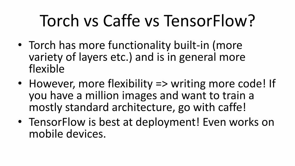
Torch vs Caffe vs TensorFlow? • Torch has more functionality built-in (more
variety of layers etc.) and is in general more flexible
• However, more flexibility => writing more code! If you have a million images and want to train a mostly standard architecture, go with caffe!
• TensorFlow is best at deployment! Even works on mobile devices.

What is Caffe? Open framework, models, and worked examples for deep learning
- 600+ citations, 150+ contributors, 7,000+ stars, 4,700+ forks, >1 pull request / day average
- focus has been vision, but branching out: sequences, reinforcement learning, speech + text

So what is Caffe?
Prototype Training Deployment
All with essentially the same code!
● Pure C++ / CUDA architecture for deep learning o command line, Python, MATLAB interfaces
● Fast, well-tested code ● Tools, reference models, demos, and recipes ● Seamless switch between CPU and GPU
o Caffe::set_mode(Caffe::GPU);

Brewing by the Numbers... • Speed with Krizhevsky's 2012 model:
– 2 ms / image on K40 GPU
– <1 ms inference with Caffe + cuDNN v2 on Titan X
– 72 million images / day with batched IO
– 8-core CPU: ~20 ms/image
• 9k lines of C++ code (20k with tests)
• https://github.com/soumith/convnet-benchmarks: A pretty reliable
benchmark

Why Caffe? In one sip…
Expression: models + optimizations are plaintext schemas, not code.
Speed: for state-of-the-art models and massive data.
Modularity: to extend to new tasks and settings.
Openness: common code and reference models for reproducibility.
Community: joint discussion and development through BSD-2 licensing.

Caffe Tutorial http:/caffe.berkeleyvision.org/tutorial/

Caffe offers the ● model definitions ● optimization settings ● pre-trained weights
so you can start right away. The BVLC models are licensed for unrestricted use.
Reference Models

The Caffe Model Zoo - open collection of deep models to share innovation - VGG ILSVRC14 + Devil models in the zoo - Network-in-Network / CCCP model in the zoo
- MIT Places scene recognition model in the zoo - help disseminate and reproduce research - bundled tools for loading and publishing models Share Your Models! with your citation + license of course
Open Model Collection
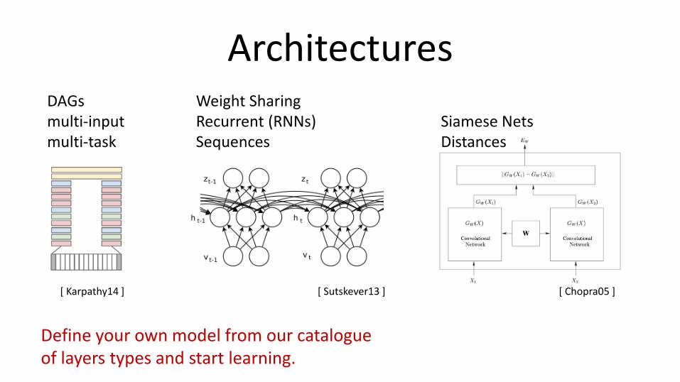
Architectures Weight Sharing Recurrent (RNNs) Sequences
Define your own model from our catalogue of layers types and start learning.
DAGs multi-input multi-task
Siamese Nets Distances
[ Karpathy14 ] [ Sutskever13 ] [ Chopra05 ]

Installation Hints
• We have already compiled the latest version of caffe (as on 5 Feb’16) on LateDays!
• However, you might want to customize and compile your own caffe (esp. if you want to create new layers)

Installation • http://caffe.berkeleyvision.org/installation.html • CUDA, OPENCV • BLAS (Basic Linear Algebra Subprograms): operations like matrix
multiplication, matrix addition, both implementation for CPU(cBLAS) and GPU(cuBLAS). provided by MKL(INTEL), ATLAS, openBLAS, etc.
• Boost: a c++ library. > Use some of its math functions and shared_pointer. • glog,gflags provide logging & command line utilities. > Essential for
debugging. • leveldb, lmdb: database io for your program. > Need to know this for
preparing your own data. • protobuf: an efficient and flexible way to define data structure. > Need to
know this for defining new layers.

TRAINING AND FINE-TUNING

Training: Step 1 Create a lenet_train.prototxt
Data Layers Loss

Training: Step 2 Create a lenet_solver.prototxt
train_net: "lenet_train.prototxt" base_lr: 0.01 momentum: 0.9 weight_decay: 0.0005 max_iter: 10000 snapshot_prefix: "lenet_snapshot" # … and some other options …

Training: Step 2
Some details on SGD parameters
𝑉𝑡+1 = µ𝑉𝑡 − 𝜶(𝛻𝐿 𝑊𝑡 + 𝝀𝑊𝑡) 𝑊𝑡+1 = 𝑊𝑡 + 𝑉𝑡+1
Momentum LR Decay

Training: Step 3
Train!
$ build/tools/caffe train \ -solver lenet_solver.prototxt \ -gpu 0

Dogs vs. Cats top 10 in 10 minutes
Fine-tuning Transferring learned weights to kick-start models
● Take a pre-trained model and fine-tune to new tasks [DeCAF]
[Zeiler-Fergus] [OverFeat]
© kaggle.com
Your Task
Style Recognition
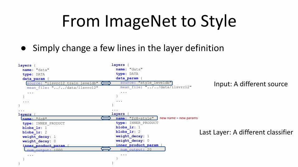
From ImageNet to Style
● Simply change a few lines in the layer definition
Input: A different source
Last Layer: A different classifier
layers {
name: "data"
type: DATA
data_param {
source: "ilsvrc12_train_leveldb"
mean_file: "../../data/ilsvrc12"
...
}
...
}
...
layers {
name: "fc8"
type: INNER_PRODUCT
blobs_lr: 1
blobs_lr: 2
weight_decay: 1
weight_decay: 0
inner_product_param {
num_output: 1000
...
}
}
layers {
name: "data"
type: DATA
data_param {
source: "style_leveldb"
mean_file: "../../data/ilsvrc12"
...
}
...
}
...
layers {
name: "fc8-style"
type: INNER_PRODUCT
blobs_lr: 1
blobs_lr: 2
weight_decay: 1
weight_decay: 0
inner_product_param {
num_output: 20
...
}
}
new name = new params

$ caffe train -solver models/finetune_flickr_style/solver.prototxt \
-gpu 0 \
-weights bvlc_reference_caffenet.caffemodel
Under the hood (loosely speaking): net = new Caffe::Net( "style_solver.prototxt");
net.CopyTrainedNetFrom(
pretrained_model);
solver.Solve(net);
From ImageNet to Style

When to Fine-tune? A good first step! - More robust optimization – good initialization helps - Needs less data - Faster learning
State-of-the-art results in - recognition - detection - segmentation
[Zeiler-Fergus]

Learn the last layer first - Caffe layers have local learning rates: blobs_lr - Freeze all but the last layer for fast optimization
and avoiding early divergence. - Stop if good enough, or keep fine-tuning
Reduce the learning rate - Drop the solver learning rate by 10x, 100x - Preserve the initialization from pre-training and avoid thrashing
Fine-tuning Tricks

DEEPER INTO CAFFE

DAG
Many current deep models have linear structure
but Caffe nets can have any directed acyclic graph (DAG) structure. Define bottoms and tops and Caffe will connect the net.
LRCN joint vision-sequence model
GoogLeNet Inception Module
SDS two-stream net

Net
name: "dummy-net"
layers { name: "data" …}
layers { name: "conv" …}
layers { name: "pool" …}
… more layers …
layers { name: "loss" …}
● A network is a set of layers connected as a DAG:
LogReg ↑
LeNet →
ImageNet, Krizhevsky 2012 →
● Caffe creates and checks the net from the definition.
● Data and derivatives flow through the net as blobs – a an array interface

Forward / Backward the essential Net computations
Caffe models are complete machine learning systems for inference and learning. The computation follows from the model definition. Define the model and run.

Layer name: "conv1"
type: "Convolution"
bottom: "data"
top: "conv1"
convolution_param {
num_output: 20
kernel_size: 5
stride: 1
weight_filler {
type: "xavier"
}
}
name, type, and the connection structure
(input blobs and output blobs)
layer-specific
parameters
* Nets + Layers are defined by protobuf schema ● Every layer type defines
- Setup - Forward - Backward

Setup: run once for initialization. Forward: make output given input. Backward: make gradient of output - w.r.t. bottom - w.r.t. parameters (if needed)
Layer Protocol
Layer Development Checklist
Model Composition The Net forward and backward passes are the composition the layers’.
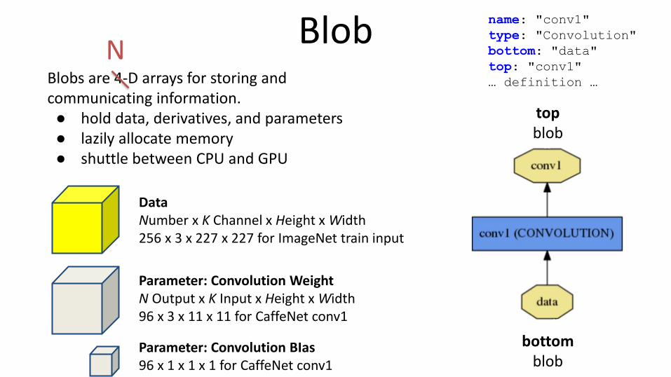
Data Number x K Channel x Height x Width 256 x 3 x 227 x 227 for ImageNet train input
Blobs are 4-D arrays for storing and communicating information. ● hold data, derivatives, and parameters ● lazily allocate memory ● shuttle between CPU and GPU
Blob name: "conv1"
type: "Convolution"
bottom: "data"
top: "conv1"
… definition …
top blob
bottom blob
Parameter: Convolution Weight N Output x K Input x Height x Width 96 x 3 x 11 x 11 for CaffeNet conv1
Parameter: Convolution BIas 96 x 1 x 1 x 1 for CaffeNet conv1
N

Blobs provide a unified memory interface.
Reshape(num, channel, height, width) - declare dimensions - make SyncedMem -- but only lazily allocate
Blob
cpu_data(), mutable_cpu_data() - host memory for CPU mode gpu_data(), mutable_gpu_data() - device memory for GPU mode
{cpu,gpu}_diff(), mutable_{cpu,gpu}_diff() - derivative counterparts to data methods - easy access to data + diff in forward / backward
SyncedMem allocation + communication
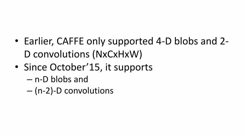
• Earlier, CAFFE only supported 4-D blobs and 2-D convolutions (NxCxHxW)
• Since October’15, it supports – n-D blobs and – (n-2)-D convolutions

A Caffe Net
Input Blob caffe::Net Output Blob
Blob: all your data, derivatives, and parameters.
● example input blob (256 images, RGB, height, width)
○ ImageNet training batches: 256 x 3 x 227 x 227
● example convolutional parameter blob
○ 96 filters with 3 input channels: 96 x 3 x 11 x 11


Can also have..
BLOB
LAYER
In-place updates

Example: ReLU or PReLU
θ
(PReLU) He et al. ICCV’15

How much memory would a PReLU require?
• It does an in-place update, so say requires 𝐵 for blob
• Say it requires 𝑃 for parameters (could be per-channel, or just a single scalar)
• Does it need any more?
– Yes! Need to keep the original input around for computing the derivative for parameters => +𝐵
• Q: Can parameterized layers do in-place updates?

GPU/CPU Switch with Blob
• Use synchronized memory
• Mutable/non-mutable determines whether to copy. Use of mutable_* may lead to data copy
• Rule of thumb:
Use mutable_{cpu|gpu}_data whenever possible

Layers

More about Layers
• Data layers
• Vision layers
• Common layers
• Activation/Neuron layers
• Loss layers

Data Layers • Data enters through data layers -- they lie at the bottom of nets.
• Data can come from efficient databases (LevelDB or LMDB),
directly from memory, or, when efficiency is not critical, from files on disk in HDF5/.mat or common image formats.
• Common input preprocessing (mean subtraction, scaling, random cropping, and mirroring) is available by specifying
TransformationParameters.

Data Layers • Data (Backend: LevelDB,LMDB)
• MemoryData
• HDF5Data
• ImageData
• WindowData
• DummyData
• Write your own! In Python!

Data Layers

Data Layers
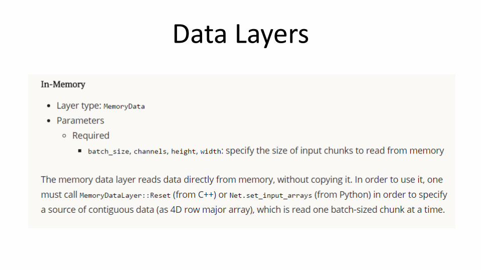
Data Layers


Writing your own data layer in python
• Compile CAFFE, uncommenting in Makefile.config
# WITH_PYTHON_LAYER := 1
• Example: See Fast-RCNN

Python Prototxt import caffe
class RoIDataLayer(caffe.Layer):
"""Fast R-CNN data layer used for training."""
def setup(self, bottom, top):
"""Setup the RoIDataLayer."""
# ...
pass
def forward(self, bottom, top):
# ...
pass
def backward(self, top, propagate_down, bottom):
"""This layer does not propagate gradients."""
pass
def reshape(self, bottom, top):
"""Reshaping happens during the call to fwd."""
pass
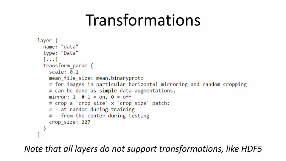
Transformations
Note that all layers do not support transformations, like HDF5

More about Layers
• Data layers
• Vision layers
• Common layers
• Activation/Neuron layers
• Loss layers

Vision Layers • Images as input and produce other images as output. • Non-trivial height h>1 and width w>1. • 2D geometry naturally lends itself to certain decisions
about how to process the input. – Since Oct’15, supports nD convolutions
• In particular, most of the vision layers work by applying a particular operation to some region of the input to produce a corresponding region of the output.
• In contrast, other layers (with few exceptions) ignore the spatial structure of the input, effectively treating it as “one big vector” with dimension “chw”.

Convolution Layer


Pooling Layer

Vision Layers
• Convolution
• Pooling
• Local Response Normalization (LRN)
• Im2col -- helper

More about Layers
• Data layers
• Vision layers
• Common layers
• Activation/Neuron layers
• Loss layers

Common Layers • INNER_PRODUCT WTx+b (fully connected) • SPLIT
• FLATTEN
• CONCAT
• SLICE
• ELTWISE (element wise operations) • ARGMAX
• SOFTMAX
• MVN (mean-variance normalization)


More about Layers
• Data layers
• Vision layers
• Common layers
• Activation/Neuron layers
• Loss layers

Activation/Neuron layers
• One Input Blob
• One Output Blob
– Both same size
• Or a single blob – in-place updates

Activation/Neuron layers
• ReLU / PReLU
• Sigmoid
• Tanh
• Absval
• Power
• BNLL (binomial normal log likelihood)


More about Layers
• Data layers
• Vision layers
• Common layers
• Activation/Neuron layers
• Loss layers

Loss
What kind of model is this?
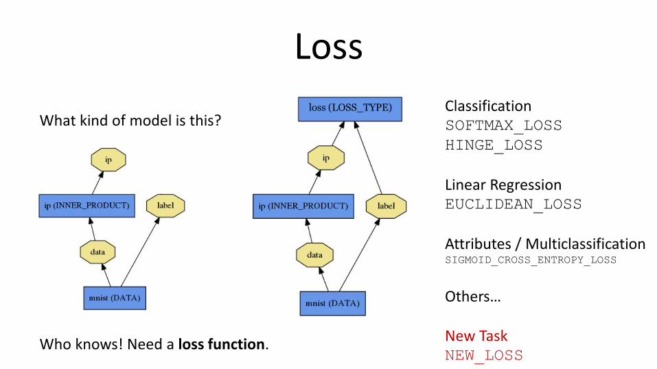
Classification SOFTMAX_LOSS
HINGE_LOSS
Linear Regression EUCLIDEAN_LOSS
Attributes / Multiclassification SIGMOID_CROSS_ENTROPY_LOSS
Others… New Task NEW_LOSS
Loss
What kind of model is this?
Who knows! Need a loss function.
loss (LOSS_TYPE)

● Loss function determines the learning task. ● Given data D, a Net typically minimizes:
Loss
Data term: error averaged over instances
Regularization term: penalize large weights
to improve generalization

Loss
● The data error term is computed by Net::Forward
● Loss is computed as the output of Layers ● Pick the loss to suit the task – many different
losses for different needs

Loss Layers • SOFTMAX_LOSS
• HINGE_LOSS
• EUCLIDEAN_LOSS
• SIGMOID_CROSS_ENTROYPY_LOSS
• INFOGAIN_LOSS
• ACCURACY
• TOPK

Loss Layers • SOFTMAX_LOSS
• HINGE_LOSS
• EUCLIDEAN_LOSS
• SIGMOID_..._LOSS
• INFOGAIN_LOSS
• ACCURACY
• TOPK
• **NEW_LOSS**
Classification
Linear Regression Attributes /
Multiclassification Other losses
Not a loss

Softmax Loss Layer
● Multinomial logistic regression: used for predicting a single class of K mutually exclusive classes
layers {
name: "loss"
type: "SoftmaxWithLoss"
bottom: "pred"
bottom: "label"
top: "loss"
}
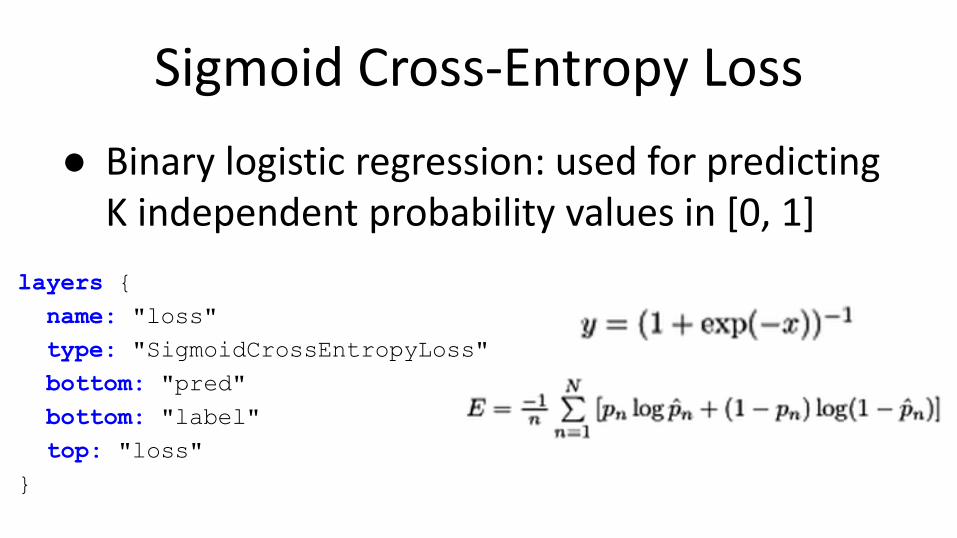
Sigmoid Cross-Entropy Loss
● Binary logistic regression: used for predicting K independent probability values in [0, 1]
layers {
name: "loss"
type: "SigmoidCrossEntropyLoss"
bottom: "pred"
bottom: "label"
top: "loss"
}

Euclidean Loss
● A loss for regressing to real-valued labels [-inf, inf]
layers {
name: "loss"
type: "EuclideanLoss"
bottom: "pred"
bottom: "label"
top: "loss"
}

Multiple loss layers
● Your network can contain as many loss functions as you want, as long as it is a DAG!
● Reconstruction and Classification:
layers {
name: "recon-loss"
type: "EuclideanLoss"
bottom: "reconstructions"
bottom: "data"
top: "recon-loss"
}
layers {
name: "class-loss"
type: "SoftmaxWithLoss"
bottom: "class-preds"
bottom: "class-labels"
top: "class-loss"
}

Multiple loss layers
“*Loss” layers have a default loss weight of 1
layers {
name: "loss"
type: "SoftmaxWithLoss"
bottom: "pred"
bottom: "label"
top: "loss"
}
layers {
name: "loss"
type: "SoftmaxWithLoss"
bottom: "pred"
bottom: "label"
top: "loss"
loss_weight: 1.0
}
==

layers {
name: "recon-loss"
type: "EuclideanLoss"
bottom: "reconstructions"
bottom: "data"
top: "recon-loss"
}
layers {
name: "class-loss"
type: "SoftmaxWithLoss"
bottom: "class-preds"
bottom: "class-labels"
top: "class-loss"
loss_weight: 100.0
}
Multiple loss layers
● Give each loss its own weight ● E.g. give higher priority to
classification error ● Or, to balance the values of
different loss functions
100*

layers {
name: "diff"
type: "Eltwise"
bottom: "pred"
bottom: "label"
top: "diff"
eltwise_param {
op: SUM
coeff: 1
coeff: -1
}
}
layers {
name: "loss"
type: "EuclideanLoss"
bottom: "pred"
bottom: "label"
top: "euclidean_loss"
loss_weight: 1.0
}
Any layer can produce a loss! ● Just add loss_weight: 1.0 to have a
layer’s output be incorporated into the loss
layers {
name: "loss"
type: "Power"
bottom: "diff"
top: "euclidean_loss"
power_param {
power: 2 }
# = 1/(2N)
loss_weight: 0.0078125 }
==
E = || pred - label ||^2 / (2N) diff = pred - label E = || diff ||^2 / (2N)
+
Layers
• Data layers
• Vision layers
• Common layers
• Activation/Neuron layers
• Loss layers

Initialization
• Gaussian [most commonly used]
• Xavier
• Constant [default]
• Goal: keep the variance roughly fixed
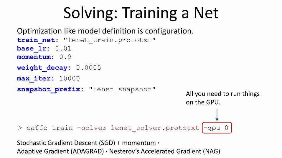
Solving: Training a Net Optimization like model definition is configuration. train_net: "lenet_train.prototxt"
base_lr: 0.01
momentum: 0.9
weight_decay: 0.0005
max_iter: 10000
snapshot_prefix: "lenet_snapshot" All you need to run things on the GPU.
> caffe train -solver lenet_solver.prototxt -gpu 0
Stochastic Gradient Descent (SGD) + momentum · Adaptive Gradient (ADAGRAD) · Nesterov’s Accelerated Gradient (NAG)


● Coordinates forward / backward, weight updates, and scoring.
● Solver optimizes the network weights W to minimize the loss L(W) over the data D
Solver

● Computes parameter update , formed from o The stochastic error gradient o The regularization gradient o Particulars to each solving method
Solver

● Stochastic gradient descent, with momentum
● solver_type: SGD
SGD Solver
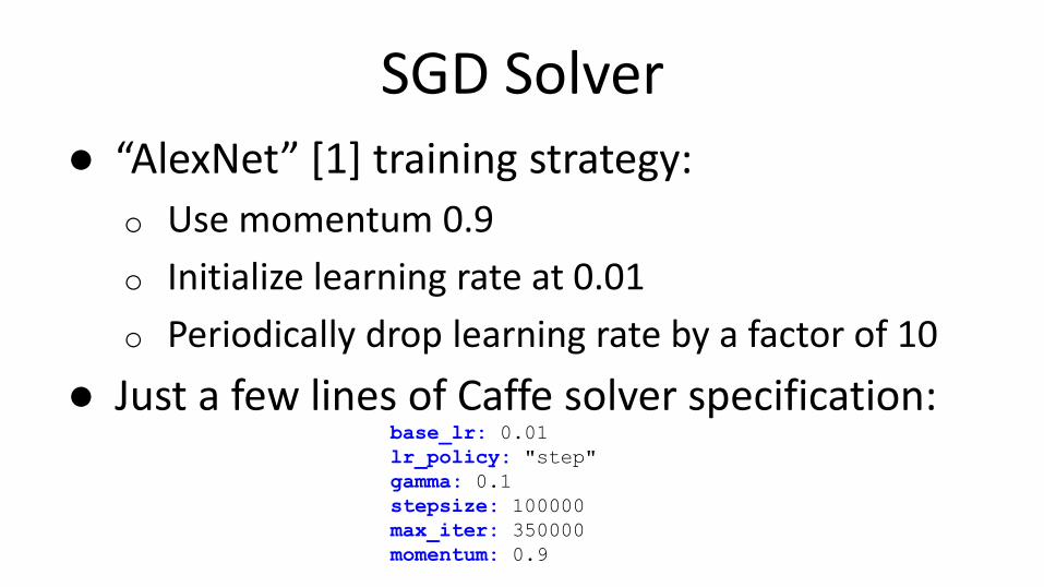
● “AlexNet” [1] training strategy:
o Use momentum 0.9
o Initialize learning rate at 0.01
o Periodically drop learning rate by a factor of 10
● Just a few lines of Caffe solver specification:
SGD Solver
base_lr: 0.01
lr_policy: "step"
gamma: 0.1
stepsize: 100000
max_iter: 350000
momentum: 0.9
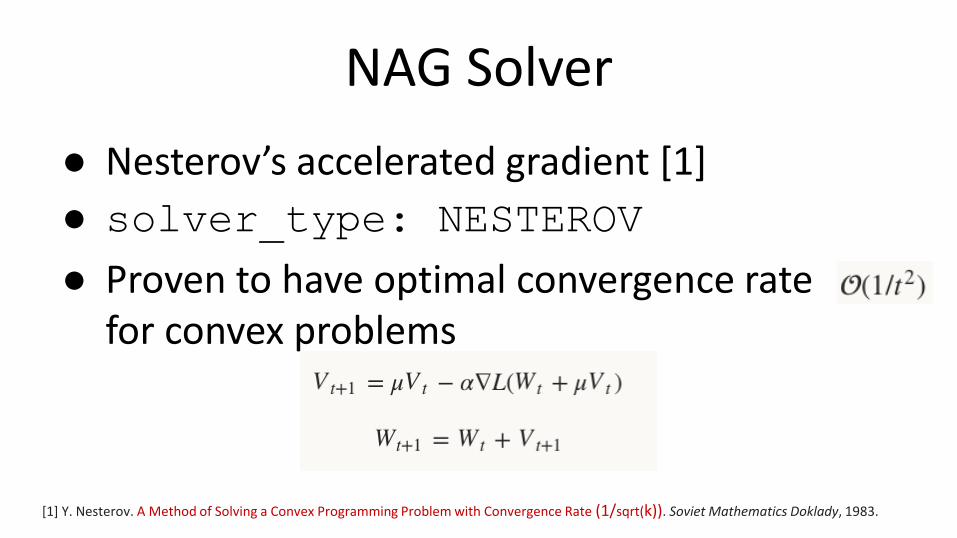
● Nesterov’s accelerated gradient [1]
● solver_type: NESTEROV
● Proven to have optimal convergence rate for convex problems
[1] Y. Nesterov. A Method of Solving a Convex Programming Problem with Convergence Rate (1/sqrt(k)). Soviet Mathematics Doklady, 1983.
NAG Solver

● Adaptive gradient (Duchi et al. [1])
● solver_type: ADAGRAD
● Attempts to automatically scale gradients based on historical gradients
AdaGrad Solver
[1] J. Duchi, E. Hazan, and Y. Singer. Adaptive Subgradient Methods for Online Learning and Stochastic Optimization. The Journal of Machine Learning Research, 2011.

I0901 13:36:30.007884 24952 solver.cpp:232] Iteration 65000, loss = 64.1627
I0901 13:36:30.007922 24952 solver.cpp:251] Iteration 65000, Testing net (#0) # train set
I0901 13:36:33.019305 24952 solver.cpp:289] Test loss: 63.217
I0901 13:36:33.019356 24952 solver.cpp:302] Test net output #0: cross_entropy_loss = 63.217 (* 1 = 63.217 loss)
I0901 13:36:33.019773 24952 solver.cpp:302] Test net output #1: l2_error = 2.40951
AdaGrad SGD Nesterov
I0901 13:35:20.426187 20072 solver.cpp:232] Iteration 65000, loss = 61.5498
I0901 13:35:20.426218 20072 solver.cpp:251] Iteration 65000, Testing net (#0) # train set
I0901 13:35:22.780092 20072 solver.cpp:289] Test loss: 60.8301
I0901 13:35:22.780138 20072 solver.cpp:302] Test net output #0: cross_entropy_loss = 60.8301 (* 1 = 60.8301 loss)
I0901 13:35:22.780146 20072 solver.cpp:302] Test net output #1: l2_error = 2.02321
I0901 13:36:52.466069 22488 solver.cpp:232] Iteration 65000, loss = 59.9389
I0901 13:36:52.466099 22488 solver.cpp:251] Iteration 65000, Testing net (#0) # train set
I0901 13:36:55.068370 22488 solver.cpp:289] Test loss: 59.3663
I0901 13:36:55.068410 22488 solver.cpp:302] Test net output #0: cross_entropy_loss = 59.3663 (* 1 = 59.3663 loss)
I0901 13:36:55.068418 22488 solver.cpp:302] Test net output #1: l2_error = 1.79998
Solver Showdown: MNIST Autoencoder

Weight sharing
● Parameters can be shared and reused across Layers throughout the Net
● Applications:
o Convolution at multiple scales / pyramids o Recurrent Neural Networks (RNNs) o Siamese nets for distance learning

Weight sharing
● Just give the parameter blobs explicit names using the param field
● Layers specifying the same param name will share that parameter, accumulating gradients accordingly
layers: {
name: 'innerproduct1'
type: "InnerProduct"
inner_product_param {
num_output: 10
bias_term: false
weight_filler {
type: 'gaussian'
std: 10
}
}
param: 'sharedweights'
bottom: 'data'
top: 'innerproduct1'
}
layers: {
name: 'innerproduct2'
type: "InnerProduct"
inner_product_param {
num_output: 10
bias_term: false
}
param: 'sharedweights'
bottom: 'data'
top: 'innerproduct2'
}

Interfaces
• Command Line
• Python
• Matlab

CMD
$> Caffe --params

CMD

CMD

Python $> make pycaffe
python> import caffe
caffe.Net: is the central interface for loading, configuring, and
running models.
caffe.Classsifier & caffe.Detector for convenience
caffe.SGDSolver exposes the solving interface.
caffe.io handles I/O with preprocessing and protocol buffers.
caffe.draw visualizes network architectures.
Caffe blobs are exposed as numpy ndarrays for ease-of-use and
efficiency**

Python
GOTO: IPython Filter Visualization Notebook

MATLAB

- Network-in-Network (NIN) - GoogLeNet - VGG
RECENT MODELS

THAT’S ALL! THANKS! Questions?

Network-in-Network
- filter with a nonlinear composition instead of a linear filter
- 1x1 convolution + nonlinearity
- reduce dimensionality, deepen the representation
Linear Filter CONV
NIN / MLP filter 1x1 CONV

GoogLeNet
- composition of multi-scale dimension-reduced “Inception” modules
- 1x1 conv for dimensionality reduction - concatenation across filter scales - multiple losses for training to depth
“Inception” module

VGG
- 3x3 convolution all the way down... - fine-tuned progression of deeper models - 16 and 19 parameter layer variations
in the model zoo
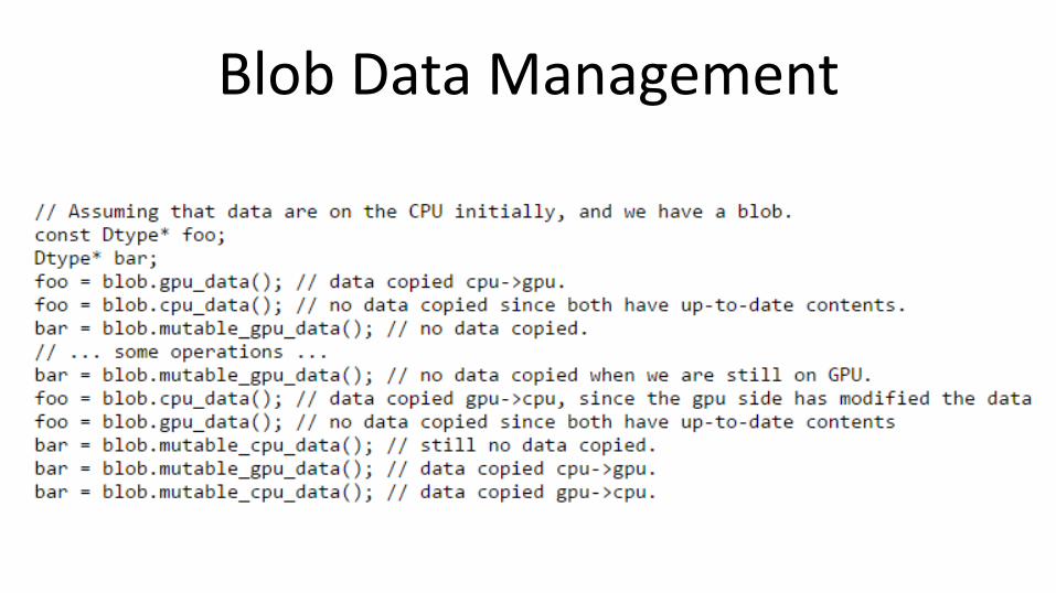
Blob Data Management