cal maritime senior design project - department … maritime... · cal maritime senior design...
TRANSCRIPT
1
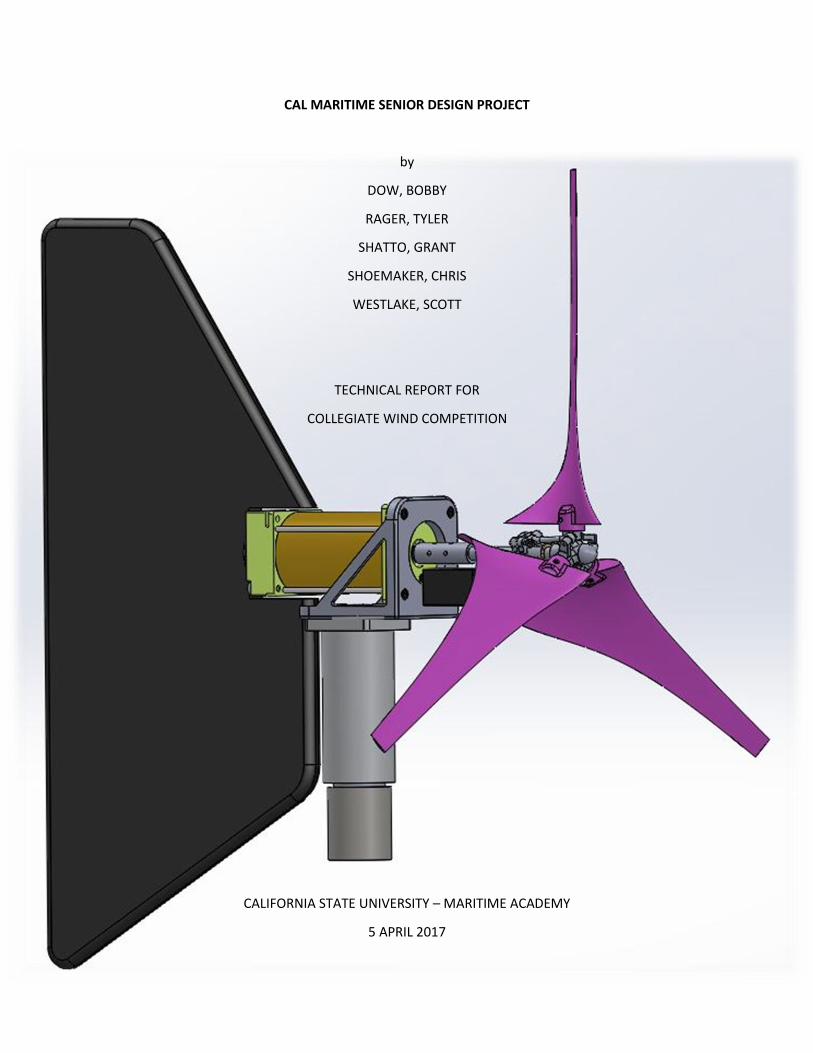
CAL MARITIME SENIOR DESIGN PROJECT
by
DOW, BOBBY
RAGER, TYLER
SHATTO, GRANT
SHOEMAKER, CHRIS
WESTLAKE, SCOTT
TECHNICAL REPORT FOR
COLLEGIATE WIND COMPETITION
CALIFORNIA STATE UNIVERSITY – MARITIME ACADEMY
5 APRIL 2017

2
Table of Contents
Table of Contents .............................................................................................................. 2
Executive Summary ........................................................................................................... 3
Chapter 1: Blades .............................................................................................................. 5
1.1 Overview ............................................................................................................ 5
1.2 Blade Features .................................................................................................... 5
1.3 Blade Design Process ........................................................................................... 5
1.4 Blade Loading...................................................................................................... 8
1.5 Final Blade Selection ............................................................................................ 9
1.6 Blade Manufacturing ......................................................................................... 10
Chapter 2: Variable Pitch and Drivetrain ........................................................................... 11
Chapter 3: Passive Yaw .................................................................................................... 13
Chapter 4: Nacelle ........................................................................................................... 14
Chapter 5: Electronics ...................................................................................................... 15
Chapter 6: Controls ......................................................................................................... 21
6.1 Controller ......................................................................................................... 21
6.2 Control Scheme ................................................................................................. 21
Chapter 7: Testing ........................................................................................................... 24
Bibliography…………………………………………………………………………………………………………………………25
3
Executive Summary
Our turbine is a three bladed, horizontal axis, upwind, direct drive system. The aerodynamic design is
based on the E 216 airfoil. The primary design and analysis tools used for creating the blades was done
through QBlade. Relatively little information exists for airfoil performance at low Reynolds Numbers;
XFoil analsys in QBlade will be the basis for predictions of aerodynamic performance. The Schmitz
Optimization theory was used to produce the chord and twist schedules for the blades. The airfoil
geometry was reconstructed in Solidworks, 3D printed with PLA, and wrapped in carbon fiber.
Theoretical analysis has blades running at a Cp of 4.7 and a TSR of 4. An analysis was done to make sure
the strength of the blades was appropriate. Start up speeds for the wind turbine occurs at a wind speed
of approximately 2.4 m/s. The theoretical power produced from the blades will be about 60Watts at a
wind speed of 11 meters per second.
The drivetrain uses a variable pitch mechanism and turbine control follow the same strategy used by
industry utility scale variable pitch, variable speed, and wind turbines. The TSR is maintained by
electronic control to achieve maximum power and variable pitch regulates power above rated wind
speeds. The variable pitch mechanism is built into the drivetrain and the shaft is directly coupled to the
generator. The variable pitch mechanism, shaft, and motor mounting plate were both designed and
precision machined by the team. The machining process involved work on the lathe, mill, and CNC
machines.
The turbine is designed using a passive yaw system that includes a large tail fin and a double bearing
sleeved assemble to allow for ease of wind tracking. The tail is connected to the nacelle through a
carbon fiber shaft. The nacelle is an open type lightweight design that allows for easy accessibility of the
generator.
The generator is a four pole brushless DC motor and was chosen because of its low cogging torque
characteristics. It’s rated speed and voltage is 3950 RPM and 38.2 volts respectively. A three phase full
wave rectifier converts AC to DC and was designed using 6 Schottky diodes and a smoothing capacitor.
At the heart of our electronics is a non-inverting Buck/Boost DC-DC converter. The voltage gain (k) can
be adjusted according to the duty cycles of the MOSFET. A gain of less than one corresponds to a Buck
mode and a gain more than one corresponds to Boost mode. The battery will hold the outlet side of the
Buck/Boost converter at a constant value of roughly 14 volts. The power generation by the turbine is
optimized by automatically adjusting the voltage gain (k) to operate its maximum power point for any
given wind speed.

4
Instrumentation in the final design includes voltage dividers for voltage measurement and Hall effect
type current sensors for current measurement. The RPM measurement is accomplished by way of an
encoder built directly into our generator. The microcontroller used in our application is a Sunfounder
Mega. The Mega was chosen for its pulse width modulation (PWM) capabilities required for the
Buck/Boost circuit, as the necessary PWM libraries are only compatible with the Mega. The final circuit
was designed in Eagle and milled on double sided copper board.
The turbine was tested in the CMA Wind Tunnel where capabilities for testing yaw were added to the
wind tunnel. Our turbine is able to return to the upwind direction when the base is rotated, while still
producing positive power. Our results generally followed our theoretical trend predicted, however the
actual power produced was significantly lower than predicted. Our theoretical model predicted about 50
Watts at 2000 RPM, whereas the turbine actually produced about 20 Watts at 2000 RPM through
testing. This did not come as a surprise because the theoretical results were intended for larger
application modeling, and did not take into account losses in the drivetrain, generator, or electronics.

5
Chapter 1: Blades
1.1 Overview
Blades capture the power of the wind and transform it to rotational power that can be used to power a
generator. The blades of the wind turbine need to be designed to be light and slim, yet strong and
durable enough to withstand the stresses produced from the high rotational speeds and pressure
differences across the blade. The blades need to be designed so that they can start up at low wind
speeds, overcoming the initial starting torque produced from the generator while achieving optimum
power output at high rotational speeds. This year’s turbine design will incorporate a horizontal axis 3
bladed upwind turbine. The turbine rotor blade design and manufacturing process is a continuous cycle
with new blades being produced continuously.
1.2 Blade Features
The blades are designed with a custom blade mount that will allow for ease of testing new and
improved designs. The blades are designed thicker near the base to aid in structural support and
stiffness of the overall blades. Two thirds of each blade will be carbon fiber wrapped from the tip down
towards the base to aid in strength and reduce deflection near the blade’s tip. This will allow for better
aero performance at high rotational speeds.
1.3 Blade Design Process
Most of the blade design is done in QBlade, an open source software created by Technical University of
Berlin that allows for wind turbine calculations [11]. QBlade uses a mixture of XFOIL, XFLR5, and BEM
modeling tools that allow for blade analysis to predict their performance. The blades are then
reconstructed in SolidWorks where a custom blade mount is placed at the root.
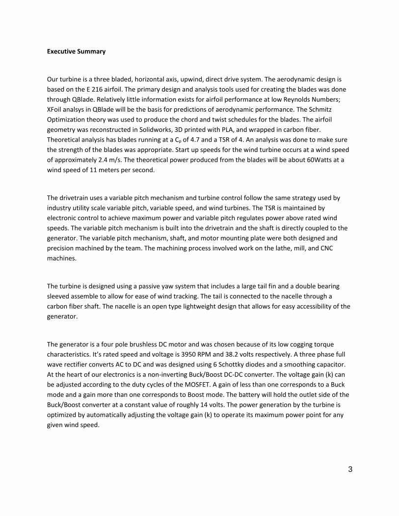
The blade design process is outlined in the flow chart of Figure 1.1. The blade design starts by choosing a
primary airfoil that will be used for most of the blade. The airfoil is chosen for its thickness, low levels of
camber, and high lift to drag characteristics. Each chosen airfoil’s geometry is imported from
airfoiltools.com [1]. Not much data is available for airfoils operating at low Reynolds numbers, so we
have to rely on the XFOIL analysis in QBlade to predict each airfoil’s behavior.
6
Figure 1.1 Blade design process flow chart
The most current blade design contains the E 216 airfoil as its most prominent airfoil. Figure 1.2 shows
the airfoil analysis made from QBlade. The airfoil’s performance from the analysis will decide whether
the airfoil will be chosen or disregarded for a better option. The analysis shows the airfoil’s optimum
angle of attack, which will allow for the blade’s twist and chord schedules to be prescribed. For the
current main outboard airfoil (the E 216) the lift to drag ratio is about 42 at an angle of attack of 7
degrees. The twist and chord for each airfoil along the blade length is produced from the Schmitz
optimization theory. Schmitz optimization theory is described in Wind Energy Explained [9] and is ideal
for horizontal axis wind turbines with wake rotation. The Schmitz optimization is calculated though a
MatLab code where a variety of the blade’s parameters can be altered; such as the blade’s tip chord
length. The middle plot in Figure 1.2 shows the moment coefficient, which will be important for
determining how much torque will have to be exerted by the actuator to change the blade’s pitch angle.
Figure 1.2 QBlade airfoil analysis of E 216 and Eppler 403 at Reynolds Number of 50,000

7
A theoretical blade is then produced in the QBlade software where the optimum chord and twist
schedules can be manipulated. QBlade allows for a blade element momentum (BEM) simulation where
different theoretical results of the blade’s performance can be analyzed. The most prominent
parameters that will be observed from this analysis are the rotor coefficient of power, (which gives an
idea of how much power the blade will be able to produce) the torque produced by the blades, and the
theoretical power and speed that the blades will be experiencing.
The figures below show the theoretical performances of the most recent blade design in QBlade. Figure
1.3 shows that the current blade design will produce a Cp of about 0.47 when designed with a tip speed
ratio of 4. Figure 1.3 also shows how effective varying pitch is in reducing power. Figure 1.4 shows the
torque produced at various pitch angles (each color line represents a new pitch angle) at start up. At a
pitch angle of 30 degrees, (blue line) the blades are able to produce enough torque to overcome the
static forces needed to turn generator (dashed blue line). The wind turbine will start to produce power
at low wind speeds of about 2.4 meters per second, assuming there are no losses in the drive train
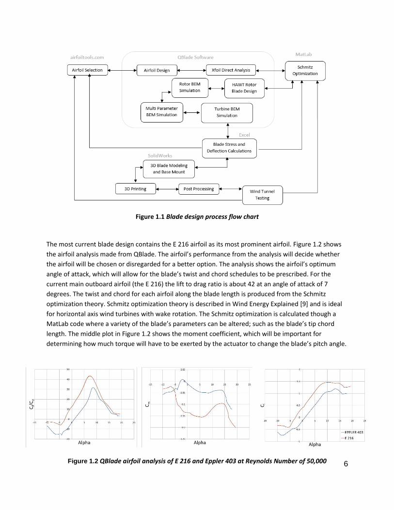
leading to the generator. Figure 1.5 shows the estimated rotational speed of the wind turbine as the
wind speed increases. It is assumed that from start up to rated power, the pitch will be set to 0 degrees
and the electronic (Buck/Boost) control of the generator will maintain an optimal tip speed ratio to
maximize Cp. The rotational speed flat-lines at a speed of about 2300 revolutions per minute due to the
pitch control of the turbine above 11 meters per second to maintain a constant power output. Figure 1.6
shows the corresponding pitch angle needed in order to maintain this constant power output. Figure
1.7 shows the amount of power that can be produced at each wind speed (i.e., the power curve).
Through pitch control, the maximum theoretical power output that will be achieved will be about 60
Watts. The theoretical results produced from the QBlade software are designed for larger application
turbines and will vary from the actual results produced from the real blades, however the results will
give guidelines for what to expect from the real blades. The QBlade analyses also neglect all mechanical
and electrical losses found in the drivetrain, generator, and electronic controls.
Figure 1.3 Coefficient of power vs. Tip
Speed Ratio at different pitch angles
Figure 1.4 Startup rotor torque produced
vs. wind speed at different pitch angles
8
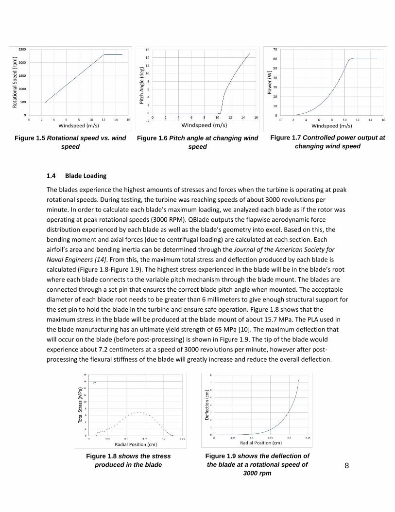
1.4 Blade Loading
The blades experience the highest amounts of stresses and forces when the turbine is operating at peak
rotational speeds. During testing, the turbine was reaching speeds of about 3000 revolutions per
minute. In order to calculate each blade’s maximum loading, we analyzed each blade as if the rotor was
operating at peak rotational speeds (3000 RPM). QBlade outputs the flapwise aerodynamic force
distribution experienced by each blade as well as the blade’s geometry into excel. Based on this, the
bending moment and axial forces (due to centrifugal loading) are calculated at each section. Each
airfoil’s area and bending inertia can be determined through the Journal of the American Society for
Naval Engineers [14]. From this, the maximum total stress and deflection produced by each blade is
calculated (Figure 1.8-Figure 1.9). The highest stress experienced in the blade will be in the blade’s root
where each blade connects to the variable pitch mechanism through the blade mount. The blades are
connected through a set pin that ensures the correct blade pitch angle when mounted. The acceptable
diameter of each blade root needs to be greater than 6 millimeters to give enough structural support for
the set pin to hold the blade in the turbine and ensure safe operation. Figure 1.8 shows that the
maximum stress in the blade will be produced at the blade mount of about 15.7 MPa. The PLA used in
the blade manufacturing has an ultimate yield strength of 65 MPa [10]. The maximum deflection that
will occur on the blade (before post-processing) is shown in Figure 1.9. The tip of the blade would
experience about 7.2 centimeters at a speed of 3000 revolutions per minute, however after post-
processing the flexural stiffness of the blade will greatly increase and reduce the overall deflection.
Figure 1.5 Rotational speed vs. wind
speed
Figure 1.7 Controlled power output at
changing wind speed
Figure 1.9 shows the deflection of
the blade at a rotational speed of
3000 rpm
Figure 1.8 shows the stress
produced in the blade
Figure 1.6 Pitch angle at changing wind
speed
9
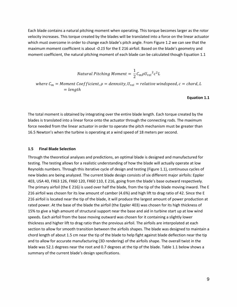
Each blade contains a natural pitching moment when operating. This torque becomes larger as the rotor
velocity increases. This torque created by the blades will be translated into a force on the linear actuator
which must overcome in order to change each blade’s pitch angle. From Figure 1.2 we can see that the
maximum moment coefficient is about -0.15 for the E 216 airfoil. Based on the blade’s geometry and
moment coefficient, the natural pitching moment of each blade can be calculated though Equation 1.1
𝑁𝑎𝑡𝑢𝑟𝑎𝑙 𝑃𝑖𝑡𝑐ℎ𝑖𝑛𝑔 𝑀𝑜𝑚𝑒𝑛𝑡 = 1
2𝐶𝑚𝜌𝑈𝑟𝑒𝑙
2𝑐2𝐿
𝑤ℎ𝑒𝑟𝑒 𝐶𝑚 = 𝑀𝑜𝑚𝑒𝑛𝑡 𝐶𝑜𝑒𝑓𝑓𝑖𝑐𝑖𝑒𝑛𝑡, 𝜌 = 𝑑𝑒𝑛𝑛𝑠𝑖𝑡𝑦, 𝑈𝑟𝑒𝑙 = 𝑟𝑒𝑙𝑎𝑡𝑖𝑣𝑒 𝑤𝑖𝑛𝑑𝑠𝑝𝑒𝑒𝑑, 𝑐 = 𝑐ℎ𝑜𝑟𝑑, 𝐿
= 𝑙𝑒𝑛𝑔𝑡ℎ
Equation 1.1
The total moment is obtained by integrating over the entire blade length. Each torque created by the
blades is translated into a linear force onto the actuator through the connecting rods. The maximum
force needed from the linear actuator in order to operate the pitch mechanism must be greater than
16.5 Newton’s when the turbine is operating at a wind speed of 18 meters per second.
1.5 Final Blade Selection
Through the theoretical analyses and predictions, an optimal blade is designed and manufactured for
testing. The testing allows for a realistic understanding of how the blade will actually operate at low
Reynolds numbers. Through this iterative cycle of design and testing (Figure 1.1), continuous cycles of
new blades are being analyzed. The current blade design consists of six different major airfoils: Eppler
403, USA 40, FX63 126, FX60 120, FX60 110, E 216, going from the blade’s base outward respectively.
The primary airfoil (the E 216) is used over half the blade, from the tip of the blade moving inward. The E
216 airfoil was chosen for its low amount of camber (4.6%) and high lift to drag ratio of 42. Since the E
216 airfoil is located near the tip of the blade, it will produce the largest amount of power production at
rated power. At the base of the blade the airfoil (the Eppler 403) was chosen for its high thickness of
15% to give a high amount of structural support near the base and aid in turbine start up at low wind
speeds. Each airfoil from the base moving outward was chosen for it containing a slightly lower
thickness and higher lift to drag ratio than the previous airfoil. The airfoils are interpolated at each
section to allow for smooth transition between the airfoils shapes. The blade was designed to maintain a
chord length of about 1.5 cm near the tip of the blade to help fight against blade deflection near the tip
and to allow for accurate manufacturing (3D rendering) of the airfoils shape. The overall twist in the
blade was 52.1 degrees near the root and 0.7 degrees at the tip of the blade. Table 1.1 below shows a
summary of the current blade’s design specifications.

10
Table 1.1
1.6 Blade Manufacturing
The blades are produced from a 3D printer (MPCNC) [15] to form their basic shape and profile out of
PLA plastic. The 3D print renders the basic blade shape that was designed for performance and can be
seen in Figure 1.10. The blades are sanded down to a smooth finish where the blades can then be post-
processed and strengthened. Two-thirds of each blade is carbon fiber wrapped from the tip towards the
base of the blade. The carbon fiber is made from a sleeve that is able to form-fit the profile of the blade
to maintain aerodynamic performance. The carbon fiber is hardened on with an epoxy resin and vacuum
bagged to meet the blade’s shape. The carbon fiber sleeve helps the blade fight against any deflection
near the blades tip, helping each blade’s performance at higher rotational speeds. The base of the blade
below the carbon sleeve will have an epoxy coat to maintain uniform blade thickness from the carbon
fiber wrap and aid in extra strength to the blade near the root.
Blade design Specifications
Radial Pos. (cm)
Chord (cm)
Twist (deg)
Airfoil
1.3 9.45 52.1 EPPLER 403
3.7 6.75 30.9 USA 403
6.0 4.97 19.9 FX63 126
8.4 3.66 12.5 FX60 120
10.7 3.01 8.9 FX60 110 13.1 2.45 5.9 E 216
15.4 2.09 3.9 E 216 17.8 1.83 2.6 E 216 20.1 1.52 1.7 E 216
22.5 1.50 0.7 E 216
Figure 1.10 shows a blade being printed

11
Chapter 2: Variable Pitch and Drivetrain
Figure 2.1 Variable Pitch Mechanism Component Labeling Front View
Figure 2.2 Variable Pitch Mechanism Component Labeling Rear View
The variable pitch mechanism allows for direct control of the blade pitch for the turbine, and is used primarily during start up, power regulation, and braking procedures. During start up, the blades are pitched to bring the turbine up to power producing speeds effectively. During full run operation the pitch remains constant, and thus the variable pitch mechanism is not actuated from its run position. During power regulation operations the pitch will be reduced by retracting the linear actuator to maintain constant power production at wind speeds above 11 m/s. The variable pitch system is comprised of a main hub, pitch driver, a push plate assembly, three blade mounts, three connecting rods, bushings, a radial bearing, fastening hardware, and a linear actuator, shown in Figure 2.1 and Figure 2.2.

12
Each of the blade mounts is fixed to the main hub with shoulder screws that wear on pressed bushings. There are two bushings inside of each blade mount and three bushings in the main hub. This allows each blade mount shoulder screw to wear on three individual bushing surfaces, avoiding any aluminum-to-aluminum contact. The blade mounts are allowed to rotate a maximum of 90 degrees, with full run position at a 20mm linear actuator arm extension. The linear actuator used is a PQ-12P Actuonix with a gear ratio of 100:1 to allow for adequate pushing and pulling forces to pitch the blades at higher wind speeds [11].
The connecting rods are fastened with shoulder screws and bushings between the lever arm of the blade mount and the pitch driver arms, and translate the linear motion of the pitch driver to angular rotation of the blade mounts. As the push plate is forced by the linear actuator the pitch driver is moved linearly along the shaft. The push plate assembly is mounted to the outer race of the radial bearing that surrounds the pitch driver. This bearing is pressed on and secured by a circlip that sits on the outer body of the pitch driver. The push plate assembly is a non-rotating portion of the variable pitch assembly, while the pitch driver rotates inside by way of the radial bearing. The maximum pushing and pulling forces calculated to pitch the blades did not warrant the need for a thrust bearing in this position, and thus a lower rolling resistance bearing was used.
Due to the minimal length, seen in Figure 2.3, and weight of the variable pitch assembly the shaft is directly coupled to the generator shaft, with no need for a support shaft bearing. The shaft and coupling are one cohesive part that was hand turned to size. The majority of the other components that comprise the variable pitch assembly were machined through a combination of hand and CNC lathe/mill work. Sometimes, the process would involve turning stock by hand, 3D machining on the CNC, and then finalizing rounds by hand, again on the lathe. First the aluminum stock was turned down by hand on the lathe. Next, the piece was set in an indexing collet in the CNC mill so that it could be rotated for 3D machining and tapping. The final steps were then done by hand and involved facing the excess stock, reaming it to fit the shaft, shaping the nose, and drilling/tapping set screw holes.
Figure 2.3 Mechanical Drawing of the Variable Pitch Mechanism

13
Chapter 3: Passive Yaw
The yaw was designed as a passive system that uses a bearing assembly with a tail to turn the turbine
into the direction of the wind. The bearing system seen in Figure 3.2 shows an exploded view of the
assembly. Two flange bearings are used in order to minimize the effect of any moments acting on the
assembly from the chasis. The yaw sleeve is made from 6061 aluminum while the yaw shaft is made
from low-carbon steel. The yaw shaft threads onto the tower with ¾’’ NPT threads.
The tail is constructed from high density foam and attches to a hole in the chasis with a carbon fiber rod
as seen in Figure 3.1. The tail was designed to have the greatest surface area possible while being within
the overall size limitations of the tubine.
An analysis of the yaw system performance was conducted using a wind tunnel and a rotating base pate.
The system was found to start working at wind speeds of aproximately 4.5 m/s, which is lower than the
competition wind tunnel’s minimum of 6 m/s during the durability test. When rotating the turbine two
full revolutions, the wires running through the turbine tower did not twist significantly.
Figure 3.2 Yaw bearing and Sleeve Figure 3.1 Turbine Tail

14
Chapter 4: Nacelle
The nacelle for the turbine features an open design. This allows the generator to remain accessible and
cool while running at high wind speeds. The design features a lightweight aluminum uni-body
construction in order to achieve maximum strength. The generator fits into the hole in the faceplate and
is secured with four socket head screws as seen in Figure 4.1. The yaw sleeve mounts to the base of the
nacelle, also with four socket head screws. The tail of the turbine mounts to the hole in the back of the
nacelle with a press fit. The main design goal of the nacelle was to make it as small as possible in order
to minimize any air flow disruption to the tail. The major dimensions can be found in Figure 4.2.
Figure 4.1 Faceplate
Figure 4.2 Faceplate Dimensions

15
Chapter 5: Electronics
The electronics can be broken down into five modular components: three phase generator; three phase
full wave rectifier; main DC-DC converter board; microcontroller; and 12V battery. The schematic is
located at the end of this section.
The generator is a 4-pole brushless DC motor manufactured by Pittman Amatek. The model number is
544S102-SP. The generator was chosen because of its low cogging torque characteristic and Kφ value.
Cogging torque refers to the amount of rotational resistance due to magnetic attraction between the
poles of the rotor and the stator. The rated speed and rated voltage are 3950 RPM and 38.2 V and are
used to calculate the Kφ value as shown below in Equation 5.1. [7] The Kφ value was then confirmed
when we tested our motor on our dynamometer.
𝐾∅ = 𝑅𝑎𝑡𝑒𝑑 𝑅𝑃𝑀
𝑅𝑎𝑡𝑒𝑑 𝑉=
3950 𝑅𝑃𝑀
38.2 𝑉 ≈ 103
𝑅𝑃𝑀
𝑉
Equation 5.1
The three phase full wave rectifier was designed with six Schottky diodes and a smoothing capacitor.
The diodes are rated for 5 continuous amps, 60 V, and a forward voltage drop of roughly 550 mV at 25
°C. The capacitor is rated at 63 V and 150 µF. The Schottky diodes were specifically chosen for their low
forward voltage drop characteristic.
The main DC-DC converter board consists of a Buck/Boost DC-DC converter in addition to inlet and
outlet current and voltage measurement devices. The Buck/Boost converter steps DC voltage either up,
or down, depending on the duty cycles of the MOSFETS. The voltage out of the Buck/Boost converter
will be held constant, roughly 14V to allow the load, a 12V battery, to charge. By adjusting the duty cycle
of the MOSFETs, the voltage gain seen on the output of the Buck/Boost converter is also adjusted. A
gain of more than 1 is defined as Boost mode and a gain of less than 1 is defined as Buck mode.
𝐺𝑎𝑖𝑛 𝑘 =𝑉𝑜𝑢𝑡
𝑉𝑖𝑛 ∴ 𝑉𝑖𝑛 =
𝑉𝑜𝑢𝑡
𝑘
Equation 5.2
In reference to Equation 5.2, as k decreases, Vin increases, and therefore so does the speed of the
generator, because Kφ and Vout are constant values. Conversely, as k increases, Vin decreases, as well as
the speed of the generator. The duty cycles of the MOSFETs are as follows in Equation 5.3 and Equation
5.4 and are defined as the percentage of time the MOSFET gate is closed.

16
𝐵𝑢𝑐𝑘 𝑚𝑜𝑑𝑒 𝑑𝑢𝑡𝑦 𝑐𝑦𝑐𝑙𝑒 𝐷 = 𝑉𝑜𝑢𝑡
𝑉𝑖𝑛
Equation 5.3
𝐵𝑜𝑜𝑠𝑡 𝑚𝑜𝑑𝑒 𝑑𝑢𝑡𝑦 𝑐𝑦𝑐𝑙𝑒 𝐷 = 1 − 𝑉𝑖𝑛
𝑉𝑜𝑢𝑡
Equation 5.4
The basic Buck/Boost converter, shown below in Figure 5.1, consists of two N-channel MOSFETS acting
as switches, two Schottky diodes, one inductor, and a smoothing capacitor. Both MOSFETs are rated at
60 V, drain to source breakdown, and 50 continuous amps. The Schottky diodes are identical to those
used in the three phase rectifier. The inductor and capacitor are sized using Equation 5.5 and Equation
5.6, below.
Figure 5.1 Basic Buck/Boost DC-DC converter with N-Channel MOSFETs
Inductor and output Capacitor sizing for rated voltage:
𝐿 = 𝑉𝑜𝑢𝑡 × (𝑉𝑖𝑛 − 𝑉𝑜𝑢𝑡)
∆𝐼𝐿 × 𝑓𝑠 × 𝑉𝑖𝑛=
14𝑉 × (30𝑉 − 14𝑉)
0.35 × 2.5𝐴 × 50000𝐻𝑧 × 30𝑉 ≈ 171 𝜇𝐻
𝑤ℎ𝑒𝑟𝑒 𝐼 = 𝑖𝑛𝑑𝑢𝑐𝑡𝑜𝑟 𝑠𝑖𝑧𝑒, ∆𝐼𝐿 = 𝑟𝑖𝑝𝑝𝑙𝑒 𝑐𝑢𝑟𝑟𝑒𝑛𝑡, 𝑎𝑛𝑑 𝑓𝑠 = 𝑠𝑤𝑖𝑡𝑐ℎ𝑖𝑛𝑔 𝑓𝑟𝑒𝑞𝑢𝑒𝑛𝑐𝑦
Equation 5.5
𝐶𝑜𝑢𝑡𝑚𝑖𝑛 = ∆𝐼𝐿
8 × 𝑓𝑠 × ∆𝑉𝑜𝑢𝑡=
0.35 × 2.5𝐴
8 × 50000 𝐻𝑧 × 0.025𝑉 ≈ 88 𝜇𝐹
𝑤ℎ𝑒𝑟𝑒 ∆𝑉𝑜𝑢𝑡 = 𝑑𝑒𝑠𝑖𝑟𝑒𝑑 𝑜𝑢𝑡𝑝𝑢𝑡 𝑟𝑖𝑝𝑝𝑙𝑒 𝑣𝑜𝑙𝑡𝑎𝑔𝑒
Equation 5.6
NOTE: ∆𝐼𝐿 is defined as (0.2 to 0.4)*(Ioutmax). [5]
NOTE: ∆𝑉𝑜𝑢𝑡 is a chosen quantity. As this quantity decreases, a larger capacitor is required.
Inductor and capacitor size used in the on the final circuit board: 180 µH & 100 μF.
To use the MOSFETs as switches, the gates of each MOSFET must be actuated by MOSFET drivers.
Drivers chosen for this application are model number IR2104 and manufactured by International
17
Rectifier. These drivers actuate the gates using a combination of a 12V DC source signal along with a
pulse width modulation (PWM) signal from a microcontroller. For this application, the PWM signal is 50
kHz, and is the switching frequency in Equation 5.5 and Equation 5.6 above.
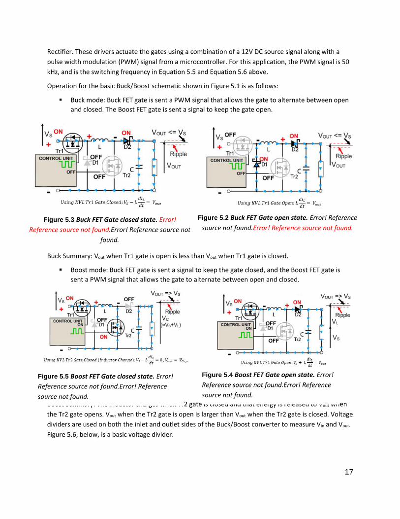
Operation for the basic Buck/Boost schematic shown in Figure 5.1 is as follows:
Buck mode: Buck FET gate is sent a PWM signal that allows the gate to alternate between open
and closed. The Boost FET gate is sent a signal to keep the gate open.
Buck Summary: Vout when Tr1 gate is open is less than Vout when Tr1 gate is closed.
Boost mode: Buck FET gate is sent a signal to keep the gate closed, and the Boost FET gate is
sent a PWM signal that allows the gate to alternate between open and closed.
Boost Summary: The inductor charges when Tr2 gate is closed and that energy is released to Vout when
the Tr2 gate opens. Vout when the Tr2 gate is open is larger than Vout when the Tr2 gate is closed. Voltage
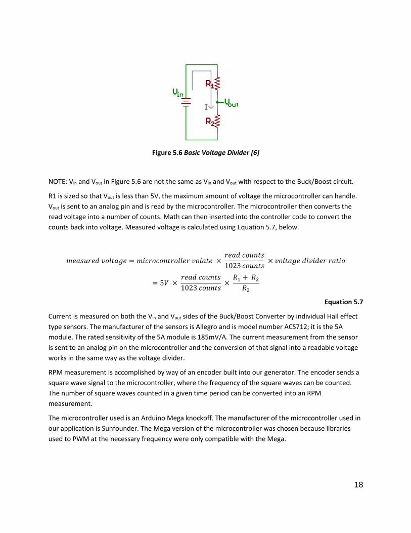
dividers are used on both the inlet and outlet sides of the Buck/Boost converter to measure Vin and Vout.
Figure 5.6, below, is a basic voltage divider.
Figure 5.3 Buck FET Gate closed state. Error!
Reference source not found.Error! Reference source not
found.
Figure 5.2 Buck FET Gate open state. Error! Reference
source not found.Error! Reference source not found.
Figure 5.5 Boost FET Gate closed state. Error!
Reference source not found.Error! Reference
source not found.
Figure 5.4 Boost FET Gate open state. Error!
Reference source not found.Error! Reference
source not found.
18
Figure 5.6 Basic Voltage Divider [6]
NOTE: Vin and Vout in Figure 5.6 are not the same as Vin and Vout with respect to the Buck/Boost circuit.
R1 is sized so that Vout is less than 5V, the maximum amount of voltage the microcontroller can handle.
Vout is sent to an analog pin and is read by the microcontroller. The microcontroller then converts the
read voltage into a number of counts. Math can then inserted into the controller code to convert the
counts back into voltage. Measured voltage is calculated using Equation 5.7, below.
𝑚𝑒𝑎𝑠𝑢𝑟𝑒𝑑 𝑣𝑜𝑙𝑡𝑎𝑔𝑒 = 𝑚𝑖𝑐𝑟𝑜𝑐𝑜𝑛𝑡𝑟𝑜𝑙𝑙𝑒𝑟 𝑣𝑜𝑙𝑎𝑡𝑒 × 𝑟𝑒𝑎𝑑 𝑐𝑜𝑢𝑛𝑡𝑠
1023 𝑐𝑜𝑢𝑛𝑡𝑠 × 𝑣𝑜𝑙𝑡𝑎𝑔𝑒 𝑑𝑖𝑣𝑖𝑑𝑒𝑟 𝑟𝑎𝑡𝑖𝑜
= 5𝑉 × 𝑟𝑒𝑎𝑑 𝑐𝑜𝑢𝑛𝑡𝑠
1023 𝑐𝑜𝑢𝑛𝑡𝑠 ×
𝑅1 + 𝑅2
𝑅2
Equation 5.7
Current is measured on both the Vin and Vout sides of the Buck/Boost Converter by individual Hall effect
type sensors. The manufacturer of the sensors is Allegro and is model number ACS712; it is the 5A
module. The rated sensitivity of the 5A module is 185mV/A. The current measurement from the sensor
is sent to an analog pin on the microcontroller and the conversion of that signal into a readable voltage
works in the same way as the voltage divider.
RPM measurement is accomplished by way of an encoder built into our generator. The encoder sends a
square wave signal to the microcontroller, where the frequency of the square waves can be counted.
The number of square waves counted in a given time period can be converted into an RPM
measurement.
The microcontroller used is an Arduino Mega knockoff. The manufacturer of the microcontroller used in
our application is Sunfounder. The Mega version of the microcontroller was chosen because libraries
used to PWM at the necessary frequency were only compatible with the Mega.

19
Construction of the final circuit was completed in the form of a printed circuit board (PCB), and is shown
below in Figure 5.7. The circuit was designed using EAGLE and milled on a double sided, 12 oz copper
board, as shown below in Figure 5.8. The final design is roughly the size of an iPhone 6 Plus and includes
both through-hole and surface mount components.
Figure 5.7 Final PCB
Figure 5.8 Milling of the final PCB with the help of Dr. Chang-Siu

20
Figure 5.9 Theoretical Power vs. RPM plots with Voltage Gain Control
Figure 5.9 shows the theoretical Power vs. RPM plot generated using the current blade design overlaid
by voltage gain operating curves. The intersection of the solid power output curves and the gain (k)
curves gives the theoretical operating point for a specific wind speed. By varying the gain, the optimal
operating point can be found.
Figure 5.10 Electronic Schematic

21
Chapter 6: Controls
6.1 Controller
The microcontroller used is an Arduino Mega clone manufactured by Sunfounder. The Mega version of
the microcontroller was chosen because only the Mega supports a few of the libraries needed to retime
the PWM signals. The Mega board also includes a surplus of both analog and digital pins that our many
instruments will need.
6.2 Control Scheme
The control skeleton used revolves around reading instruments and changing both the pitch of the
turbine blades and the DC power converter to track power through changing wind conditions. Referring
back to Figure 1.7, the control scheme is setup to follow this peak power curve. This figure is again
shown below.
Figure 6.1 Power output at changing wind speed
0
10
20
30
40
50
60
70
0 2 4 6 8 10 12 14 16
Power(W)
Windspeed(m/s)
22
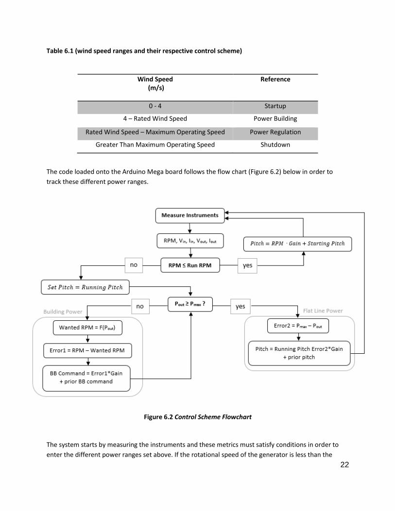
Table 6.1 (wind speed ranges and their respective control scheme)
Wind Speed (m/s)
Reference
0 - 4 Startup
4 – Rated Wind Speed Power Building
Rated Wind Speed – Maximum Operating Speed Power Regulation
Greater Than Maximum Operating Speed Shutdown
The code loaded onto the Arduino Mega board follows the flow chart (Figure 6.2) below in order to
track these different power ranges.
Figure 6.2 Control Scheme Flowchart
The system starts by measuring the instruments and these metrics must satisfy conditions in order to
enter the different power ranges set above. If the rotational speed of the generator is less than the

23
upper range of start up, the controls set the pitch of the blades to maximize torque on the generator.
Once the generator starts rotating, the RPM is used to slowly change the pitch of the blades to increase
generator RPM once again, see Figure 1.4. This loop continues to run until the generator speed reaches
the point of full run position on the pitch of the blades.
Once the blades reach full running position the pitch is locked in at 0 degrees. The wanted RPM of the
generator is a function of the power out and this function is found using data collected in the wind
tunnel manually. Once the wanted RPM is known this is used to calculate an error between the actual
RPM of the turbine and the wanted RPM based on the measured power. This error is then turned in to a
proportional command. This command is then used by the DC power converter and utilized to maximize
power output during the building range. This control is used until the system is producing the maximum
amount of power at the rated wind speed of 11 m/s.
From the rated speed of 11 m/s to maximum operational speed, the controls will lock the DC power
converter to a fixed gain while pitch regulation is accomplished using a proportional error command
between the rated power and actual power output. This command is used to maintain the correct RPM
previously reached at a wind speed of 11 m/s. This flat line power range is maintained through pitch
regulation until the maximum wind speed is reached at which point the turbine is pitched to full feather
position and shuts down.

24
Chapter 7: Testing
After assembling the different sections of the turbine and integrating the machine to the electronics and
controls the turbine was placed into the Cal Maritime wind tunnel. The wind tunnel used for testing has
a flow straightener in the entrance of the tunnel with a three-foot square test section. The fan is driven
by a variable frequency drive controller coupled to an AC motor. The tunnel can reach wind speeds up to
13 m/s as specified in the competition. A data acquisition system utilizes a pitot tube to enable the users
to measure wind speeds.
During initial testing of the turbine the machine was fixed to a rigid tower since design of a tail had not
yet been completed. These early tests allowed for analysis of initial blade designs and the feasibility of
the variable pitch mechanism. After the turbine passed these initial tests the tail was completed along
with the yaw mechanism and strengthened blades. After setting the yaw up with the rotating tower
mount, data was acquired during the power building wind speed range. The system output power was
measured with wind speeds from lowest possible start up point up to ten meters per second. Figure 7.1
shows the power curves of the operating system at fixed wind speeds and varying gains.
Figure 7.1 Power output while altering power converter settings.
By plotting these power curves at different wind speeds and varying the gain (k), the peak power
outputs at specific wind speeds were found. Fitting a theoretical third order polynomial relationship
between power and wind speed to these measured peak powers develops an equation to be used by
0
5
10
15
20
25
0 500 1000 1500 2000 2500 3000
Po
we
r (W
atts
)
RPM
Power vs Generator RPM
8m/s
5m/s
"START -2.7m/s"2.8m/s

25
the control to find the peak power autonomously. The peak power curves for the building range can be
seen below in Figure 7.2 and Figure 7.3.
Bibliography
[1] “Airfoil Tools.” Airfoil Tools. N.p., n.d. Web. 29 Mar. 2017.
[2] Bindra, Ashok. “Trade-Offs In Switching High-Input-Voltage Step-Down Converters at High Frequencies.”
Trade-Offs in Switching High-Input-Voltage |DigiKey. N.p., n.d. Web. 4 Apr. 2017.
[3] Coats, Eric. “Learnabout Electronics.” Buck-Boost Converters. N.p., n.d. Web. 04 Apr. 2017.
[4] Fundamentals of Power Electronics – Buck-Boost Coonverter Basics. Perf. Katkimshow.Youtube.N.p., n.d.
Web. 4 Apr. 2017.
[5] Hauke, Brigitte. “Basic Calculation of a Buck Converter’s Power Stage.” Texas Instruments. N.p., n.d. Web.
4 Apr. 2017.
[6] Jimbo. “Voltage Dividers.” Voltage Dividers. N.p., n.d. Web. 04 Apr. 2017.
[7] Kerk, Haydon. "Shop Haydon Kerk & Pittman - Brushless DC Motors & Gearmotors - 5443S102-
SP123." Shop Haydon Kerk & Pittman - Brushless DC Motors & Gearmotors - 5443S102-SP123. N.p., n.d.
Web. 05 Apr. 2017.
[8] Kwasinski. “DC-DC Buck Converter.” The University of Texas at Austin. Web. 4 Apr. 2017.
[9] Manwell, J. F., J. G. McGowan, and Anthony L. Rogers. Wind Energy Explained: Theory, Design and
Application. Chichester, U.K.: John Wiley & Sons, 2011. Print.
[10] PLA and ABS Strength Data (n.d.): n. pag. Makerbot. MakerBot. Web. 29 Mar. 2017.
[11] “PQ12 Linear Actuator 20mm, 100:1, 12V, Potentiometer.” Roboshop. N.p., n.d. Web. 12 Feb. 2017.
[12] “QBlade.” QBlade. N.p., n.d. Web. 29 Mar. 2017.
[13] Texas Instruments Incorporated. How to Design an Efficient Non-inverting Buck-boost Converter (n.d.): n.
pag. Texas Instruments. Web. 4 Apr. 2017
[14] “The Bending Of Inertia And Airfoil Sections.” Journal of the American Society for Naval Engineers 21.4
(2009): 1365-1368. MIT Open Course Ware. Web 30 Mar. 2017.
[15] “Vicious1.com.” Vicious Circle CNC. N.p., n.d. Web. 30 Mar. 2017.
Figure 7.2 Peak power vs. generator RPM Figure 7.3 Peak power vs. wind speed