calcium signalling of human airway epithelial calu …943809/...calcium signalling of human airway...

Calcium Signalling of Human Airway Epithelial Calu-3Cell Monolayer Induced by a Deposition of Quantum

Dots

JOHNNY ISRAELSSON JUSSI

Master of Science Thesis in Engineering PhysicsSupervisor: Dr. Huijan Yin

Examiner: Associate Professor Ying FuStockholm, Sweden 2016

TRITA-FYS 2016:41ISSN 0280-316XISRN KTH/FYS/–16:41—SE

Department of Applied PhysicsSchool of Engineering SciencesRoyal Institute of Technology

SE-100 44 StockholmSWEDEN

Akademisk avhandling som med tillstånd av Kungliga Tekniska högskolan framläg-ges till offentlig granskning för avläggande av Master of Science and EngineeringPhysics in Biomedical Physics 9 Juni, 2016 i seminarierum Pascal på SciLifeLab,Tomtebodavägen 23, Solna.

© Johnny Israelsson Jussi, June 2016

Tryck: US-AB

Abstract

Nanoparticle entry into the human body can occur by severaldifferent pathways, and the mechanisms of cell toxicity are com-plex and in need of further investigation. The respiratory systemis however considered to be the major pathway for entry, whichis why a previous study [PLoS ONE, 2, 11 (2016)] utilized col-loidal quantum dots QDs in order to investigate the effects fromrepeated depositions of QDs on human airway epithelial Calu-3cell cultures. Once every day, over a six day period, transepithe-lial electrical resistance TEER were measured during QD stim-ulation, and the measurements showed an immediate, transientdecrease of TEER, with recovery over time - without noticeablechanges over the six day period. Here, the underlying mecha-nism behind this observed phenomena have been studied throughthe use of TEER measurements and confocal laser-scanning mi-croscopy, where the focus have been on calcium signalling withthe use of Oregon Green staining. Measurements were performedon Calu-3 cells cultured either as liquid-covered culture LCC orair-interfaced culture AIC at different development phases, in thepresence and absence of calcium channel inhibitors BTP2 andNifedipine, and stimulated with 50µL QDs. TEER of LCC celllayers exhibited the same behaviour as previously shown after QDstimulation, this was found to be inhibited by BTP2, and alsowhen cells were exposed to a calcium free medium. Imaging ex-periments shows that a QD deposition on LCC cell layers induceda rapid, transient increase in intracellular calcium levels, whichBTP2 and calcium free medium inhibited. The results from usingNifedipine however indicates that it does not inhibit the response.AIC cell layers did not exhibit any response during TEER de-tection after stimulation with QDs, imaging did however show avery large morphological response, where cell death seemed to beproportional to the QD concentration. It is evident that calciumsignalling is important for the overall response of epithelial cellsin its response towards nano-scale materials.

Sammanfattning

Det finns flertalet vägar för nanopartiklar att träda in i män-niskokroppen och de mekanismerna som styr celltoxicitet är oer-hört komplexa och i behov av ytterliga studier. Den huvudsak-liga vägen för inträde anses dock vara via respirationssystemet,vilket är grundorsaken till att en tidigare studie [PLoS ONE, 2,11 (2016)] undersökte bieffekterna från att stimulera de mänskligaluftvägsceller Calu-3 vid upprepade tillfällen med kolloida kvant-prickar. Under en sexdagarsperiod mättes transepitelialt elektriskresistans (TEER) en gång per dag då QDs deponerade på celler,där mätningarna visade en omedelbar, transient minskning avTEER - med återhämtning över tid, utan märkbara förändringarunder denna sexdagarsperiod. Den underliggande mekanismen fördetta fenomen har studerats i denna rapport genom mätningar avTEER samt konfokalmikroskop, där fokus har legat på kalcium-signalering genom märkning med Oregon Green. Mätningar harutförts på Calu-3 celler som odlats med eller utan medium ovanpåcellerna (med LCC, utan AIC) vid olika utvecklingsfaser i närvaroeller frånvaro av kalciumantagonister BTP2 och Nifedipine och destimulerades med 50 µL QDs. Mätningar av TEER på LCC celleruppvisade samma beteende som i den tidigare studien efter stimu-lering av QD, detta visade sig dock bli helt blockerat då BTP2 varnärvarande, samt då celler utsattes för ett kalciumfritt medium.Stimulering med QDs på LCC celler under mätningar med kon-fokalmikrosop visade sig även inducera en mycket snabb ökning avde intracellular kalciumnivåerna, vilket återigen helt blockeradesav BTP2 och ett kalciumfritt medium. Experiment då Nifedipineanvändes visar sig dock inte blockera ökningen av kalcium. AICceller uppvisade ingen respons efter en stimulering med QDs un-der mätningar med TEER, men under konfokalmikroskop syntesen drastiskt morfologisk förändring hos cellerna efter stimuleringmed QDs, där celldöd tycktes vara proportionell mot koncentra-tionen av QDs. Det är uppenbart att kalciumsignalering är viktigtför hur epitelceller försvarar sig mot material i nanoskala.

Glossary

AIC Air Interfaced Culture.

ATP Adenosine Triphosphate.

Calu-3 Human airway Epithelial cells.

CB Conduction Band.

CFTR Cystic Fibrosis Transmembrane Conductance Regulator.

Ca-free Calcium-free Krebs-Ringer Buffer.

CRAC Calcium Release-Activated Calcium Channel.

Ca-rich Calcium-rich Krebs-Ringer Buffer.

DMSO Dimethyl Sulfoxide.

EMEM Eagle’s Minimum Essential Medium.

FBS Fetal Bovine Serum.

GM Growth mMedium

LCC Liquid Covered Culture.

3-MPA 3-Mercaptopropionic Acid.

NHERF1 Na+/H+ Exchange Regulatory Factor.

Oregon Green Oregon Green BAPTA-AM.

PBS Phosphate-buffered Saline.

v

vi GLOSSARY

PDZ Post Synaptic Density Protein, Drosophila Disc Large Tumor Suppressor andZonula Occludens-1 Protein.

P/S Penicillin and Streptomyocin.

SOCE Store-Operated Calcium Entry.

TEER Transepithelial Electrical Resistance.

TJ Tight Junction.

VB Valence Band.

QD Quantum Dot.

ZO Zonula Occludens.

Preface

The work presented in the thesis was executed at Cell Physics, Department ofApplied Physics, School of Engineering Sciences, Royal Institute of Technology,Stockholm, Sweden.

List of papers not included in the thesis

Paper 1. Study on Visual Ca2+ Signaling Induced by Mechanical Stimulation of Cdse-Cds/Zns Quantum Dot Deposition in Human Airway Epithelial Calu-3 CellMonolayerHuijuan Yin, Jacopo Fontana, Johan Solandt, Johnny Israelsson Jussi, HaoXu, Marina Zelenina, Hjalmar Brismar, Ying FuIn manuscript

Acknowledgments

I am grateful to the following peopple, and I want to give my most sincerethanks for helping me throughout this whole process:

Huijan Yin for helping me with all the cell culture maintenance and showingme how to do pipetting in a good manor.

Ying Fu for giving me the opportunity to work on this project, and helping methroughout the whole project with data processing.

A special thanks also goes out to Johan Solandt as a representative of As-trZeneca at SciLifeLab, in a consulting and supportive capacity throughout theproject.

Contents

Glossary v

Contents ix

List of Figures xi

1 Introduction 1

2 Aims & Objectives 32.1 Aims . . . . . . . . . . . . . . . . . . . . . . . . . . . . . . . . . . . . 32.2 Objectives . . . . . . . . . . . . . . . . . . . . . . . . . . . . . . . . . 3

3 Background 53.1 Respiratory barrier . . . . . . . . . . . . . . . . . . . . . . . . . . . . 5

3.1.1 Mucociliary escalators . . . . . . . . . . . . . . . . . . . . . . 53.1.2 Physical barrier and Cell junctions . . . . . . . . . . . . . . . 63.1.3 Secretion of antimicrobial substances . . . . . . . . . . . . . . 7

3.2 Barrier Assessment . . . . . . . . . . . . . . . . . . . . . . . . . . . . 73.2.1 TEER . . . . . . . . . . . . . . . . . . . . . . . . . . . . . . . 7

4 Theoretical background 94.1 Confinement and energy levels . . . . . . . . . . . . . . . . . . . . . 9

4.1.1 Quantization of energy levels . . . . . . . . . . . . . . . . . . 94.1.2 Periodic potential . . . . . . . . . . . . . . . . . . . . . . . . 104.1.3 Quantum confinement and density of states . . . . . . . . . . 11

4.2 Quantum Dots . . . . . . . . . . . . . . . . . . . . . . . . . . . . . . 15

5 Methods 195.1 Cell culture . . . . . . . . . . . . . . . . . . . . . . . . . . . . . . . . 195.2 Colloidal quantum dots . . . . . . . . . . . . . . . . . . . . . . . . . 205.3 Stimuli . . . . . . . . . . . . . . . . . . . . . . . . . . . . . . . . . . . 205.4 Cell labeling . . . . . . . . . . . . . . . . . . . . . . . . . . . . . . . . 215.5 TEER . . . . . . . . . . . . . . . . . . . . . . . . . . . . . . . . . . . 21

ix

x CONTENTS

5.6 Microscopy . . . . . . . . . . . . . . . . . . . . . . . . . . . . . . . . 225.7 Data analysis . . . . . . . . . . . . . . . . . . . . . . . . . . . . . . . 23

5.7.1 Single cell . . . . . . . . . . . . . . . . . . . . . . . . . . . . . 235.7.2 Relative Change . . . . . . . . . . . . . . . . . . . . . . . . . 24

6 Results 276.1 TEER . . . . . . . . . . . . . . . . . . . . . . . . . . . . . . . . . . . 276.2 Calcium signalling by QD deposition . . . . . . . . . . . . . . . . . . 29

6.2.1 Inhibition of either release or influx of calcium . . . . . . . . 316.2.2 Time course development . . . . . . . . . . . . . . . . . . . . 326.2.3 Inhibition measurements . . . . . . . . . . . . . . . . . . . . . 346.2.4 Distriution of the individual cell response . . . . . . . . . . . 37

6.3 AIC cultured Calu-3 cells . . . . . . . . . . . . . . . . . . . . . . . . 386.3.1 LCC compared with AIC . . . . . . . . . . . . . . . . . . . . 39

7 Discussion 41

8 Conclusion 45

Bibliography 47

A Calu-3: Culture and labeling 51A.1 Introduction . . . . . . . . . . . . . . . . . . . . . . . . . . . . . . . . 51A.2 Growth Medium . . . . . . . . . . . . . . . . . . . . . . . . . . . . . 51A.3 Culture . . . . . . . . . . . . . . . . . . . . . . . . . . . . . . . . . . 51A.4 Oregon Green BAPTA-AM Labeling . . . . . . . . . . . . . . . . . . 53

B Sample Matlab code 55B.1 Brightness.m . . . . . . . . . . . . . . . . . . . . . . . . . . . . . . . 55B.2 Img.m . . . . . . . . . . . . . . . . . . . . . . . . . . . . . . . . . . . 60B.3 Mesh.m . . . . . . . . . . . . . . . . . . . . . . . . . . . . . . . . . . 62B.4 RelChange.m . . . . . . . . . . . . . . . . . . . . . . . . . . . . . . . 63B.5 PlotEllipse.m . . . . . . . . . . . . . . . . . . . . . . . . . . . . . . . 64B.6 Colorbar.m . . . . . . . . . . . . . . . . . . . . . . . . . . . . . . . . 64

List of Figures

3.1 A model of the respiratory barrier in airway epithelium. . . . . . . . . 6

3.2 Model of TEER measurement and electrical pathways. (a) Cells aregrown on permeable membranes, which allows for access of chopstickelectrodes to apical compartment and basolateral compartments. Yield-ing possibility for measurement of TEER across the cell monolayer. (b)Generalized electrical scheme of a cell monolayer; Ra apical resistance,Rb basolateral resistance, Rtj resistance by the tight junctions, and Ricintercellular resistance. . . . . . . . . . . . . . . . . . . . . . . . . . . . 8

4.1 (a) Dispersion curve of the three lowest bands of a free electron. (b)Dispersion curve of an electron subjected to a one-dimensional periodicpotential at the boundary between the first and second band in thenearly-free electron approximation. The first band of the free electronis included as a reference. (c) Energy bands formed by the forbiddengaps. In (a) and (b), h = 1,m = 1, a = 2 and in (b) U = −0.2 . . . . . . 11

4.2 Density of states for CdSe under different confinement conditions forelectrons in the conduction band, with Ec = 0 and meff = m∗e =0.13 ∗m0 kg where m0 = 9.11 ∗ 10−31kg is the electron rest mass. (a)CdSe bulk, (b) CdSe quantum well with Lz = 10nm, (c) CdSe quantumwire with cross section 10∗10nm2, (d) CdSe quantum dot with a volumeof 10 ∗ 10 ∗ 10nm3, and Γ = 1meV . . . . . . . . . . . . . . . . . . . . . 14

4.3 Band gap development of CdSe QDs following the Brus equation 4.22,for a radius range from 1nm to ab = 5.4nm . . . . . . . . . . . . . . . . 17

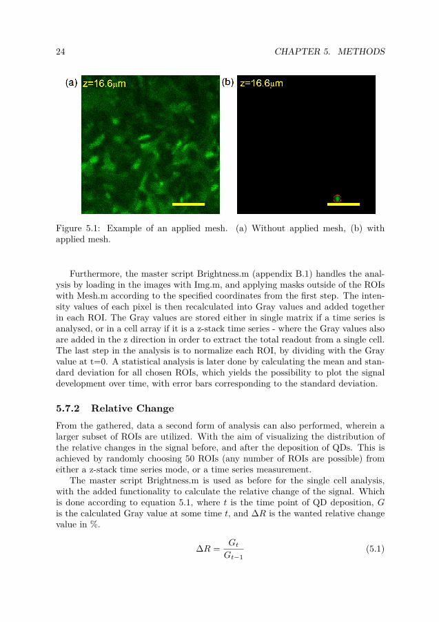
5.1 Example of an applied mesh. (a) Without applied mesh, (b) with appliedmesh. . . . . . . . . . . . . . . . . . . . . . . . . . . . . . . . . . . . . . 24

xi

xii List of Figures

6.1 TEER results from measurements on Calu-3 cells, where it is specified inthe plot what stimuli was used. (a) Six different 14 day old inserts weremeasured for 15 minutes, and a deposition of QDs or ATP occurred at5 and 10 minutes, (b) TEER development over time at different culturetimes of LCC and AIC cells, at 8, 15 and 22 days, with a deposition ofQDs after 3 and 6 minutes. The results are shown at an offset from eachother for easier interpretation. . . . . . . . . . . . . . . . . . . . . . . . . 28

6.2 TEER results from measurements on Calu-3 cells cultured 23 days ormore, where it is specified in the plot what stimuli was used. (a) 20minute measurement with QDs deposited at 5 minutes, (b) 3 insertsof different measurement times and QD deposition at the indicated reddashed lines. The results are shown at an offset from each other foreasier interpretation. . . . . . . . . . . . . . . . . . . . . . . . . . . . . . 28

6.3 Signal development plotted over time at six different z-positions on Ore-gon green labelled Calu-3 cells, with a deposition of 8µM QDs at 4 min-utes. 10 minute measurement time with a z scaling of 2.760µm. Grayvalue development of (a) Oregon green signal,(b) Bright field. Where thearrows signify the increase in z-position. Images taken (c) 30 s before,(d) directly after, (e) 30s after QD deposition. . . . . . . . . . . . . . . . 29

6.4 Signal development due to multiple depositions of 8µM QDs at the in-dicated red dashed lines, on Oregon green labelled Calu-3 cells. Ten re-gions of interest were chosen and analysis were done as per the methodin section 5.7, (a) Oregon green (b) Bright field where error bars corre-spond to the standard deviation, (c) image from the first measurementshowing an area in the middle of the cells, where the ten regions havebeen encircled, with a scale bar of 50µm. . . . . . . . . . . . . . . . . . 30

6.5 Frames from a single z-stack after multiple QD depositions when boththe green and red channel was utilized so as to image both the Oregongreen and QD at the same time. (a) image from a z-position within thecells, (b) image from a z-position above the cells, (c) enlarged orthogonalz-y view from the z-stack. 50µm scale bars. . . . . . . . . . . . . . . . . 31

6.6 Signal development due to a deposition of QDs on Oregon green labelledCalu-3 cells, with a deposition of 5µM QDs at the red dashed line. Tenregions of interest were chosen and analysis was done as per the methodin section 5.7. (a)-(c) results of Area 1, and (d)-(e) of Area 2, whereerror bars correspond to the standard deviation. The small insets areimages taken from the stacks at the noted time points, with scale bar of50µm. . . . . . . . . . . . . . . . . . . . . . . . . . . . . . . . . . . . . . 32

List of Figures xiii

6.7 Signal development at different development stages, due to a depositionof 5µM QDs at the indicated red dahsed line, on Oregon green labelledCalu-3 cells. Ten regions of interest were chosen and analysis was doneas per the method in section 5.7. Images (a)-(c) are results from cellscultured for 8 days, with a z-plane spacing of 4.8µm. Images (d)-(e) areresults from cells cultured for 15 days, with a z-plane spacing of 4.8µm.Images (g)-(i) are results from cells cultured for 23 days, with a z-planespacing of 6.4µm. The total z-range analysed was 19.2µm for all threecases. Error bars correspond to the standard deviation. . . . . . . . . . 33

6.8 Signal development due to a deposition of 5µM QDs at the red dashedline, on Oregon green labelled Calu-3 cells whilst access to calcium wasinhibited. Ten regions of interest were chosen and analysis was doneas per the method in section 5.7. Images (a)-(c) are results for whencells had been exposed to 50µM BTP2, (d)-(e) are results from whencells had been exposed to a Ca-Free (Cf-KRB) medium, and (g)-(i) areresults from when cells had been exposed to a 1µM Nifedipine. Errorbars correspond to the standard deviation. BTP2 and Ca-free measure-ments were done by time series mode, with 5s intervals between eachrecorded frame. The Nifedipine results are from a z-stack time seriesmeasurement, with 10s intervals, where this plot shows the developmentfrom one z-plane at 24.5µm. The insets correspond to a recorded imagewith the chosen ROIs encircled at the noted time, with scale bars of 50µm. 35

6.9 Oregon Green signal development due a depositions of 5µM QDs at theindicated red dashed line, on Oregon green labelled Calu-3 cells. (a)Cells in Ca-rich medium with a z-plane spacing 6.4 µm, (b) Cells in Ca-rich medium and 1µMNifedipine, with a z-plane spacing 4.9 µm. (c) and(d) corresponds to the same inserts as in (a) and (b) after normalizationto 1 was done, and the shown plot is of the mean values for this timeperiod, where error bars are of the standard deviation. . . . . . . . . . . 36

6.10 Relative changes in the Oregon Green signal by 5µM deposition of QDs,from a z-stack time series measurement, with a z-plane spacing of 6.4 µM. 37

6.11 Calcium signal and morphology of Calu-3 cells cultured using AIC in-duced by QD stimulation. Cells were imaged for a total of 5 minutesafter staining. 50µL KRB buffer (a), 25nM (b), 0.25µM(c) or 5µM(d) QDs were deposited into the insert. Overlay images with Oregongreen+Bright field are shown before (e) and after (f) stimulation, andare placed to the right of the corresponding measurement with 10 µmscale bars . . . . . . . . . . . . . . . . . . . . . . . . . . . . . . . . . . . 38

6.12 Bright field images of Calu-3 cells cultured either using LCC or AICbefore and after a deposition of QDs. LCC; (a) Before QDs, (b) after16 µM QDs. AIC; (c) Before QDs, (d) after 0.5µM QDs. . . . . . . . . . 39

Chapter 1

Introduction

Nanoparticles are gaining widespread usages for everyday life, with an increasingamount of applications in numerous areas. The entry of nanoparticles into thehuman body can occur by several pathways, such as through the skin, the gas-trointestinal tract, or the respiratory system. There is thus a need for investigatingmechanisms of cell toxicity in response to nanoparticles, where there are severalpublications that have investigated this issue in the past [1],[2]. However, there arestill questions regarding the interactions between nanoparticles and the human lungtissue, which is of great importance to further investigate due to the respiratorysystem being considered as major pathway for the entry into the human body.

Cell structure and function can in many ways be correlated to the tightness andrestrictiveness of epithelial layers and one important regulator of these characteris-tics are the tight junctions (TJ) [3]. These are critical multiprotein complexes thatcan rapidly reorganize depending on the situation at hand, and are responsible forthe regulation of paracellular diffusion [4]. Epithelial cell lines that form tight junc-tions are thus of interest to investigate in detail and specifically airway epithelialcells are the focus for this study.

Several cell lines can be used, and have been used, to model the human airway[5] and [6], but not all of them can form the needed stable tight junctions and reachconfluence under in vitro conditions [5]. The cell line of choice for this study are theHuman Arway Epithelial Calu-3 cells since it has been shown in numerous studiesthat it forms tight junctions and can easily be grown on permeable membranes.Calu-3 cells have been used in various studies in the past such as for metabolismcharacteristics [7], protein permeability [8], anion secretion [9].

In order to assess the quality of the formation of tight junctions in cell mono-layers in vitro it is common to use cells that grows as an adherent monolayer whenseeded on permeable membranes since it allows for access to the apical- and baso-lateral membranes. Transepithelial electrical resistance (TEER) is a method whereone can measure the resistance across the cellular monolayer, which is a good mea-sure of the formation of tight junctions. TEER measurements have previously been

1

2 CHAPTER 1. INTRODUCTION

used for numerous studies; TEER changes due to Nanoparticle exposure on Calu-3cells [10]; increase of TEER and enhanced barrier stability by applying glucocorti-coids on Calu-3 cells [11]; translocation of nanoparticles through Calu-3 cells whencells had been exposed to the pro-inflammatory mediator tumor necrosis factor α,which also showed a decrease in TEER [12].

This report will first focus on a continuation of a previous article from a researchgroup lead by Ying Fu from the cell physics group at KTH [13]. It was observedthere that upon deposition of 3-MPA CdSe-CdS/ZnS quantum dots (QD) ontoCalu-3 monolayer an immediate transient TEER decrease occurred. This phenom-ena was then theorized to occur due to an increase in transepithelial conductanceand current mediated by an increase of intracellular Ca2+ concentration due tomechanical stimulation of the cilium. This increase in calcium would then activatea Ca2+-activated K+ channel at the basolateral membrane, so that there is anincrease of outward potassium current − which induces an increase of chloride se-cretion by the cystic fibrosis transmembrane conductance regulator (CFTR) at theapical membrane. In this report, the effect of Ca2+ and its role in the modulationof the epithelial barrier will be investigated.

Chapter 2

Aims & Objectives

2.1 Aims

As stated earlier, it was shown in [13] that a deposition of QDs onto a monolayerof Calu-3 cells induced an immediate transient decrease in TEER. This was theo-rized to occur due to an increased intracellular Ca2+-concentration as a result ofmechanical stimulation of the cilium by the QDs.

The main aim of this project is to quantify the role that Ca2+ have with regardsto cell tightness in more detail.

2.2 Objectives

• Culture and manage Calu-3 cells from frozen storage to confluence

• Measure TEER of polarized Calu-3 cells under different conditions

• Fluorescent imaging of Ca2+ in polarized Calu-3 cells under different condi-tions

• Quantify and analyse results from TEER and fluorescent imaging

3

Chapter 3

Background

3.1 Respiratory barrier

Humans are fairly brittle constructs where the tiniest of molecule can disrupt andinjure the most vital functions. But the human body encompasses numerous pro-tective measures, such as the skin against mechanical injury for instance. Anotherprotective measure is the respiratory system whose main function is the intake andexchange of oxygen and carbon dioxide, but it also acts as sort of a barrier againstother inhaled particles. The amount of inhaled air is dependent on the amount ofphysical exertion the body is under, but a low estimate is that there is 5L/min ofair entering our lungs and thus exposing the body to particulate matters, nanopar-ticles and microbes for instance. Substances which are not supposed to pass theblood-air barrier, so an injury of some sort to this barrier may then be very serious.

The barrier of the respiratory system can in itself be divided into three dis-tinct protective measures; mucociliary escalators, cell junctions and secretion ofantimicrobial substances (see figure 3.1).

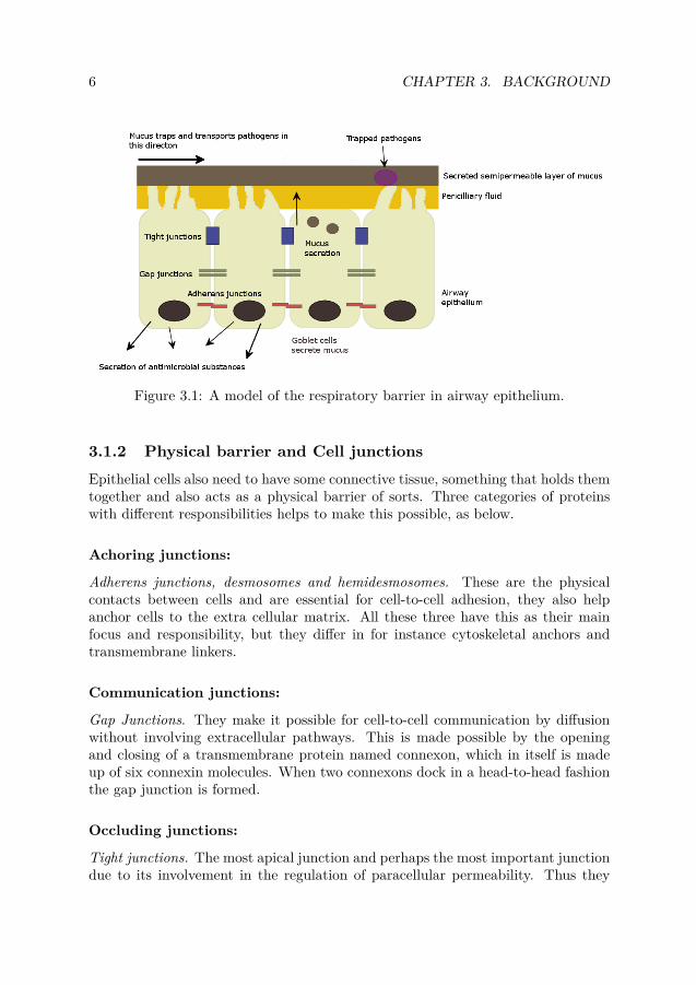
3.1.1 Mucociliary escalatorsThe mucociliary escalators, or the mucociliary apparatus or mucociliary clearence,can be divided into two parts that are essential for the others function; mucousand cilium. Where the mucus lays as a semipermeable layer on top of epithelialcells which both allows for the exchange of nutrients, water and gases whilst alsoacting as a trap for foreign pathogens. These trapped pathogens are then effec-tively removed by the continuous and coordinated beating of cilium towards thepharynx, from which the escalator moniker comes from. The mucous have a gel-likesubstance where the most important components are the mucins which are glyco-sylated proteins with a high resistance to proteolysis and are able to hold water.Secretion is done by goblet cells and submucosal glands wherein 200 proteins ofthe mucous have bee identified, such as antimicrobial substances (lysozyme anddefensins), cytokines, and antioxidant proteins [14].

5

6 CHAPTER 3. BACKGROUND

Figure 3.1: A model of the respiratory barrier in airway epithelium.

3.1.2 Physical barrier and Cell junctionsEpithelial cells also need to have some connective tissue, something that holds themtogether and also acts as a physical barrier of sorts. Three categories of proteinswith different responsibilities helps to make this possible, as below.

Achoring junctions:

Adherens junctions, desmosomes and hemidesmosomes. These are the physicalcontacts between cells and are essential for cell-to-cell adhesion, they also helpanchor cells to the extra cellular matrix. All these three have this as their mainfocus and responsibility, but they differ in for instance cytoskeletal anchors andtransmembrane linkers.

Communication junctions:

Gap Junctions. They make it possible for cell-to-cell communication by diffusionwithout involving extracellular pathways. This is made possible by the openingand closing of a transmembrane protein named connexon, which in itself is madeup of six connexin molecules. When two connexons dock in a head-to-head fashionthe gap junction is formed.

Occluding junctions:

Tight junctions. The most apical junction and perhaps the most important junctiondue to its involvement in the regulation of paracellular permeability. Thus they

3.2. BARRIER ASSESSMENT 7

restrict movement between epithelial layers, both in the apical and basolateraldirection.

3.1.3 Secretion of antimicrobial substancesThe function of the respiratory barrier is not only a physical barrier, it is alsoa major part of the immune system and its function in the fight against foreignpathogens and viruses. This is not something I intend to go into much detail inthis report, but it is still important to mention that the airway epithelium havethe ability to react both by the innate immune system but also by the adaptiveimmune system for secretion of for instance enzyme, protease inhibitors, oxidantsand antimicrobial peptides.

3.2 Barrier Assessment

The quality and integrity of physiological barriers in both epithelial and endothelialcells are highly important for their activities in various tissues of the body, andthey generally function in the same fashion wherever they are present - at least inthat the junctional complexes mediate paracellular diffusion between compartmentsof different chemical compositions. These barriers thus have implications for thetreatment of certain diseases as well, since drugs must be designed both for thetreatment but also for the specific transport across the physiological barrier inquestion to reach its target.

Cell lines that exhibit certain characteristics in vitro can be used to asses thesephysiological barriers, i.e. assess parameters that control permeability and thus atan early stage in development provide information about the transport of drugsacross a barrier. Some usual characteristics of cell lines used for theses assessmentsincludes; formation of an adherent monolayer when grown on semipermeable mem-branes; the formation of polarized cell layers; to some extent, mimic the barrierintended physiology and functionality. When such cell lines are grown on perme-able membranes, they are done so with a specific aqueous growth medium both inan apical compartment and in an basolateral compartment, yielding the possibilityto measure electrical resistance across the cell monolayer - known as TransepithelialElectrical Resistance (TEER). This is thus used as an indicator for cell tightnessand integrity of the cell monolayer.

3.2.1 TEERA crude model of the utilized setup for measuring TEER can be seen in Fig. 3.2.a.In order to utilize this type of measurement on a cell layer, it is essential thatcells have been cultured on semipermeable membranes so that there is divisionbetween/access to an apical compartment and a basolateral compartment. A cur-rent can then be applied through two electrodes which are inserted into the twocompartments, one longer in the basolateral and one shorter in the apical (without

8 CHAPTER 3. BACKGROUND

touching the cell monolayer) and the resulting resistance can be measured due tothe only thing separating the electrodes being the cell monolayer. The measuredvalues are determined by the parallel resistance arising through the transceullarand paracellular ionic pathways as in 3.1.

RTEER = Rp//Rt (3.1)

In Fig. 3.2.b, a generalized electrical pathway of such a monolayer have beendepicted, where the rectangles are resistance elements; Ra is the resistance on theapical side, Rb is the resistance on the basolateral side, Rtj is the resistance by thetight junctions, and Ric is the intercellular resistance, which leads to Rp = Rtj+Ricand Rt = Ra + Rb. These values are however proportional to the area of themembrane inserts, so the reported values are thus often as in 3.2 of the unitsWcm2, where Minsert is the area of the insert. The usage of TEER as an indicatorfor cell tightens comes from the fact that the dominating ionic pathway is theparacellular route [15]. Hence, TEER values reflects the tightness and integrity ofa cell monolayer in the form of the paracellular ionic conductance, measured in anoninvasive, real-time fashion.

TEERreported = RTEER ∗Minsert (3.2)

Figure 3.2: Model of TEER measurement and electrical pathways. (a) Cells aregrown on permeable membranes, which allows for access of chopstick electrodes toapical compartment and basolateral compartments. Yielding possibility for mea-surement of TEER across the cell monolayer. (b) Generalized electrical scheme ofa cell monolayer; Ra apical resistance, Rb basolateral resistance, Rtj resistance bythe tight junctions, and Ric intercellular resistance.

Chapter 4

Theoretical background

In order to quantify results obtained from measurements in a proper way, it iscrucial to have a working understanding of the underlying theory of the observedphenomena. Hence, this chapter will go through some of the more vital points inthe theory behind quantum dots.

4.1 Confinement and energy levels

4.1.1 Quantization of energy levelsIf one first considers electrons under spherical conditions with radiusr =

√x2 + y2 + z2, the time-independent Schrodinger equation takes the form of

4.1 when constrained by some potential U , where m is the mass of the electron,h = 6.58 ∗ 10−16 eVs is Plancks reduced constant.

EΨ(r, θ, φ) = − h

2mr2

[ ∂∂r

(r2 ∂

∂r) + 1

sin θ∂

∂θ(sin θ ∂

∂θ) + 1

sin2 θ

∂2

∂ψ2 +U(r)]Ψ(r, θ, φ)

(4.1)Then, if one considers this potential to be spherically symmetric with an infinite

barrier as in 4.2 wherein a denotes the radius of the potential.

U(r) =

0, r ≤ a.∞, r > a.

(4.2)

The solution is fairly straightforward and easily solvable by separation of thewavefunction Ψ in 4.1 into functions specifically dependent on the spherical co-ordinates as Ψ(r, θ, ψ) = R(r)Θ(θ)Φ(φ). This mathematical manipulation yieldsquantized solutions depending on three numbers (spin might also be a factor oneconsiders an applied magnetic field); principal quantum number n, the orbital num-ber l and the magnetic number m. Energy values are then quantized into different

9

10 CHAPTER 4. THEORETICAL BACKGROUND

levels as 4.3.Enl = h2χ2

nl

2ma2 (4.3)

Where χ is a spherical bessel function dependant on the quantized numbers n and l.For example, if one considers the ground state, l = 0 and χn0 = πn(n = 1, 2, 3 . . .)yields 4.4.

En0 = h2π2n2

2ma2 (4.4)

From which an important relationship can be derived by considering momentum p

and the wavenumber k; energy can be formulated by E = p2

2m and p = hk, fromwhich it is possible to relate the wavenumber to the principal qunatum number nas in 4.5.

kn = π

an (4.5)

There are of course much more detailed derivations of how this is achieved, forinstance [need reference]. But this was a simple illustration of how electrons in aninfinite potential well develops quantized energy levels.

4.1.2 Periodic potentialIf one next considers when a electrons is subjugated to a periodic potential suchas U(x) = U(x + a) so that it is invariant under translation in space by a. Wavefunctions that satisfy the Schrodinger equation with such a potential will thenonly differ in a phase factor eikx from a function which is also periodic in a, asin 4.6 for all integers n. This forms what is known as Bloch’s theorem, which inother words states that the Eigenfunctions of the Hamiltonian in this considerationrepresents a plane wave modulated by the periodicity of the potential. The subscriptk represents wavenumbers of the plane wave.

Ψk(x) = uk(r)eik·x, uk = uk(x+ an) (4.6)

A consequence of the translational symmetry is that there is no uniqueness inthe indexing of k, since both k and k+ 2nπ/a satisfies 4.6. Which also means thatthere are equivalent intervals in k as in 4.7 where each interval have a width of 2π/a.These zones are equivalent in width, but each interval encompass nonequivalent kvalues denoted as Brillouin zones.

−πa

< k <π

a; π

a< k <

3πa

; 3πa< k <

5πa

; (4.7)

A free electron have an energy-wavenumber relation as En(k) = h2k2

2m and isplotted in Fig. 4.1.a, in what is known as a dispersion curve. If the electron insteadis subjected to a periodic potential as discussed above, the relationship betweenenergy and wavenumber is much more complex and forbidden gaps can be seen inthe energy spectrum. The reason behind this is that at the boundaries between

4.1. CONFINEMENT AND ENERGY LEVELS 11

subsequent brillouin zones, there are no propagation of waves due to the forma-tion of standing waves for each k value that satisfies 4.8 with different probabilitydensities [16].

kn = π

an; n = ±1,±2,±3, . . . (4.8)

This essentially means that electrons either will be concentrated below or aboveto where the traveling wave otherwise would propagate, so that there are discon-tinuities at each point satisfying 4.8 in the relationship between wavenumber andenergy. This have been visualized in Fig. 4.1.b at the boundary between the firstand second band in the nearly-free electron approximation [17], alongside the firstband of the free electron as a comparison. In Fig. 4.1.c the corresponding energybands due to these forbidden gaps are imaged.

Figure 4.1: (a) Dispersion curve of the three lowest bands of a free electron. (b)Dispersion curve of an electron subjected to a one-dimensional periodic potentialat the boundary between the first and second band in the nearly-free electronapproximation. The first band of the free electron is included as a reference. (c)Energy bands formed by the forbidden gaps. In (a) and (b), h = 1,m = 1, a = 2and in (b) U = −0.2

4.1.3 Quantum confinement and density of statesHow energy bands are populated with electrons give insight into the electronicproperties and functions that a solid material possesses. For instance, if all valenceelectrons entirely fill up one or more bands and leave the rest empty it is denotedas an insulator since there is no way to induce a current flow. Semiconductormaterials on the other hand have energy bands which are almost entirely filled oralmost entirely empty with valence electrons, which can be utilized by an externalelectric field to move electrons and thus induce a current for instance. The highest


occupied band is called the conduction band (CB; energy Ec) and the lowest emptyband is called the valence band (VB; energy Ev). The energy difference betweenthese bands is the band gap, Eg = Ec − Ev.

Semiconductor materials can also be utilized so as to exhibit optical properties,which then have a dependency on the occupancy of electrons in each energy level.Or more precisely, on the availability of a state within an energy level to be occupiedwith electrons - which is described by something known as Density of states. BelowI shall go through how Density of states then varies for different confinements from3D to 0D. In the calculations below, it is assumed that there are periodic boundaryconditions in place as in 4.9, earlier the boundary conditions were assumed to bestatic.

Ψk(x+ Lx, y + Ly, z + Lz) = Ψk(x, y, z) (4.9)

This has implications in how the wavenumber is formulated; instead of 4.5 it takesthe form of 4.10.

ki = 2πniLi

; i = x, y, z (4.10)

3D - Bulk

In this case the consideration is essentially a 3D lattice extended in x, y, z-directionsof certain lengths - Lx, Ly, Lz. If these lengths are large enough, the system is to beconsidered as bulk. One can then imagine a sphere in k space of volume Vk = 4

3πk2

containing a multitude of energies according to 4.11. Where meff is the effectivemass.

E = hk2

2meff(4.11)

All surface points on this sphere of a certain radii have the same energy with adecrease in energy for smaller radii. The smallest volume a state can encompass ink space occurs as 4.12 with a volume Vstate = 8π3

LxLyLz.

kx = 2π/Lx; ky = 2π/Ly; kz = 2π/Lz (4.12)

By dividing the volume of one state with the total volume yields the number ofavailable states as eq. 4.13, where there is a multiplication by 2 to account for spindegeneracy.

N3D = 2VstateVk

= k3

3π2LxLyLz (4.13)

Expressing this as number of states per volume instead and considering energydensity (derivation with respect to energy) yields the density of states in 3D, 4.14.

4.1. CONFINEMENT AND ENERGY LEVELS 13

D(E)3D = dN3D

dE

1LxLyLz

= 12π2

(2meff

h2

)3/2√E (4.14)

2D - Quantum Well

Electrons are now confined along some axis, for instance Lz << Lx, Ly. This yieldsan area in k-space of different energies as Ak = πk2 with the smallest nonzero areathat one state occupies as Astate = kxky = 4π2

LxLy. The maximum number of states

encompassed by this area are then (spin degeneracy accounted for) as in 4.15.

N2D = k2

2πLxLy (4.15)

As in the 3D case, the number of states per volume for energy density yields thedensity of states in 2D. But, one also has to include the confined axis as there willbe subbands for each kz. With this consideration in mind, the 2D Density of statestakes the form of 4.16 where H is the Heaviside function.

D(E)2D = meff

h2πLz

∑nz

H(E − Enz) (4.16)

1D - Quantum Wire

Carriers are now essentially only allowed one axis of free movement over somelength, where the total length in k-space is Lk = 2k. Whereas the largest width ofone state in this k-space simply is Lstate = ki, where index i is whatever axis notunder confinement. If I choose confinement along i = x for instance, the maximumnumber of states are as in 4.17, where again spin degeneracy is accounted for.

N1D = k

πLz = 2

π

√2meffE

h2 Lz (4.17)

Which can be redefined as before to yield the density of states. Now there arehowever two axis of confinements which need be considered as well, which yieldssubbands in the confined axis’s for ky and kz. Yielding a density of states in 1D as4.18.

D(E)1D = 12πSz,y

√2meff

h2

∑ny,nz

1E − Eny,nz

H(E − Enz) (4.18)

0D - Quantum Dot

There is now confinement in all directions so that there are no axis’s that carrierscan freely move within. This means that if the confinement is infinitely small in all


directions, the density of states would take the form of dirac delta functions, as in4.19 when spin degeneracy and all confined states are considered.

D0D(E) = 2LxLyLz

∑nx,ny,nz

δ(E − Enx,ny,nz ) (4.19)

But there is always some size to this confinement and thus the quantum dot, sothis expression is then approximated as in 4.20 where Γ is the relaxation energy

D0D(E) = 2LxLyLz

∑nx,ny,nz

Γ(E − Enx,ny,nz )2 + Γ2 (4.20)

DOS summary

In figure 4.2, the resulting DOS of the four cases are plotted alongside each otherwhen electron states in the conduction band of CdSe, with an infinitely high po-tential barrier as a consideration.

Figure 4.2: Density of states for CdSe under different confinement conditions forelectrons in the conduction band, with Ec = 0 andmeff = m∗e = 0.13∗m0 kg wherem0 = 9.11 ∗ 10−31kg is the electron rest mass. (a) CdSe bulk, (b) CdSe quantumwell with Lz = 10nm, (c) CdSe quantum wire with cross section 10 ∗ 10nm2, (d)CdSe quantum dot with a volume of 10 ∗ 10 ∗ 10nm3, and Γ = 1meV

4.2. QUANTUM DOTS 15

4.2 Quantum Dots

Quantum dots are nanoscale "man-made" particles comprised of semiconductor ma-terials which exhibits quantum mechanical effects by their confinement in in all spa-tial directions. In the pretext of this thesis, so called core-shell quantum dots are ofinterest. They are comprised of type II-VI, IV-VI, or III-V semiconductor materialswith a core and either a singular shell or a multitude of shells - such as CdS/ZnS,CdSe/ZnS, CdSe/CdS, or InAs/CdSe, where it is written as core/shell. Organicsurface ligands are also usually coated and bound to the QD shell surface so as toincrease the biocompatibility, and if the QDs are to be used for specific targetingone must conjugate them to either binding peptides or antibody molecules. Duringthe latest decade or so, QDs have been gaining more attention and recognition asa viable alternative to regular organic dyes used for biomedical imaging. In com-parison to organic dyes, QDs have many attractive traits, such as broad absorptionspectra, narrow emission spectra, stable photostability, long fluorescent lifetimes,and the possibility for tailoring the emission spectra. Below, I shal go throughsome basic theory regarding semiconductor materials in general and tie it into thefunctionality of QDs so that I in the end can explain some of these attractive traits.

By the interactions between electrons and holes (empty electron states), it ispossible to derive the basics of how semiconductor material behaves. If an electronoccupying a state in the VB is excited by some external mechanism, such as theabsorption of a photon, to the CB and thus leaving a state empty in the VB, anelectron-hole pair is formed. After some relaxation time, the electron will fall backto the lower energy position in the VB. To do so requires an empty state, so byreturning to the VB, the hole state is subsequently "removed". The electron-holepair is said to recombine, which can occur in a radiative fashion by the emission ofa photon. The wavelength of the emitted photon is specific to the band gap of thematerial in use, which earlier was specified as the difference (in energy) between theVC and VB. This formulation of the band gap can be reformulated as the minimalenergy that is needed to create an electron-hole pair. Furthermore, the wavelengthof an emitted photon from bulk semiconductor, as a result of an earlier absorptionof a photon and subsequent formation of an electron-hole pair and recombination(as above), is approximately equal in energy to the band gap of the material in use- which can be formulated by the well known formula Eg = hc

λ . Where Eg is theband gap of the material, h = 4.14 ∗ 10−15eVs is plancks constant, c = 2.99 ∗ 108

ms−1 is the speed of light in vacuum, and λ is the wavelength of the emitted photon.Holes as well as electrons have charge, (holes have positive and electrons have

negative), which in turn means that there is coulombic interaction between them.By this interaction, a quasi-particle referred to as an exciton can be formed. Aparticle which have vast implications on the functionality of nanostructures, sincelight-matter interactions are stronger when the electron-hole pair are close in spacewhen the exciton is formed, [18]. An important parameter for nananostructures ingeneral is the exciton Bohr radius ab, since it describes the most probable distancebetween the electron-hole pair. The equation for it is formulated as in 4.21, where


ε0 = 8.85∗10−12 Fm−1 is the vacuum permittivity, ε∞/ε0 is the dielectric constantof the material in question, a0 = 5.29 ∗ 10−11m is the Bohr radius specifying themost probable distance between the proton and electron of the hydrogen groundstate, m0 = 9.11 ∗ 10−31 kg is the resting mass of the electron and µ = 1

m∗e+m∗

his

the reduced mass, wherein m∗e and m∗h are the effective masses of the electron andhole, respectively. If ab is comparable (i.e. smaller or slightly larger) to somenanostructure size, there is a quantization in the center-of-mass motion of theexciton which splits the energy levels in comparison to the behavior of "ordinary"electrons in a sphere for instance.

ab = ε∞ε0

m0

µa0 (4.21)

As seen in the previous section, and mentioned earlier in this one, the confine-ment in a quantum dots affects all spatial directions, the DOS thus follows the formof a δ-function (see figure 4.2 (d) as well). By this phenomena and the fact that theradii of QDs are smaller than aB , QDs have altered properties from that of regularbulk semiconductors, where the splitting of the energy levels are of one of the mostapparent ones. What this effectively means for QDs, is a direct correlation betweenthe radius of QDs to the ensuing band gap. This correlation were first put intonumbers through the Brus Equation [19] as in 4.22, which is valid for the groundelectron-hole state (1s1s), wherein r is the radius of the QD, q = 1.60 ∗ 10−19 C isthe elementary charge, and Ebulkg is the band gap of the bulk material.

EQDg = Ebulkg + h2

8r2

[ 1m∗e

+ 1m∗h

]− 1.768q2

4πε0ε∞r(4.22)

The quantum dots used in this thesis have a CdSe core, hence it is fitting toutilize the properties of such QDs in an example of the Brus equation equation. So,the properties of CdSe QDs can be seen in table 4.1, and by using these parametersin equation 4.22 it is possible to at least gain an inkling as for how the size mayaffect the band gap and thus the resulting photon emission wavelength and energy.

CdSeEg[eV ] 1.74ab[nm] 5.4m∗e/m0 0.13m∗h/m0 0.45ε∞/ε0 10.16

Table 4.1: Basic parameters for Cadmium selenide quantum dots at 300K.

The only parameter left to decide is the radius, where an appropriate range isbetween 1nm to ab. The resulting band gap development when such a range ischosen can be seen in figure 4.3. This shows that by decreasing the radius of theQD, the band gap increases along with it. So there is a direct correlation between

4.2. QUANTUM DOTS 17

decreasing the QD radius and increasing the energy of an emitted photon. Thisis however only an approximation where, for instance, shell contributions are notaccounted for, and it is expected to fail for very small nanocrystals.

Figure 4.3: Band gap development of CdSe QDs following the Brus equation 4.22,for a radius range from 1nm to ab = 5.4nm

Chapter 5

Methods

5.1 Cell culture

Human airway epithelial Calu-3 cells were purchased from ATCC (ATCC HTB-55TM), and is the cell line of use throughout this report as they form adherent,polarized monolayers [20] with tight junctions when cultured on semi-permeablepolyester membranes. This is a so called immortalized cell line, meaning that itis possible to culture them over prolonged periods of time in vitro, due to somemutation that causes the cells being able to proliferate indefinitely - where themutation for the Calu-3 cells is caused by cancerous means as they originates froma patient with bronchial adenocarcinoma. Cells of passage 6-9 were used for theseexperiments.

The entirety of how the preparation of the Calu-3 cells were done for this reportcan be found in appendix A.3. In short though, cells were prepared from frozenstorage and cultured in ATCC-formulated Eagle’s Minimum Essential Medium(EMEM, ATCC 30-2003), and supplemented with 10% Fetal Bovine Serum (FBS)and 100 units/ml of Penicillin and 100µg/mL Streptomyocin (P/S). Cells wereinitially cultured on petri dishes to an optimal confluency of 75-90% (as per theprotocol here [20] which was closely followed, with a few slight alterations) in anincubator set to 37°C in a humidified atmosphere of 5% CO2. When cultured tothe desired level of confluence, cells were seeded into cell culture Transwell-Clearinserts (6-well clusters, 24-mm inserts with polyester membrane, pore diameter 0.4µm, Corning NY)) at a density of 4 ∗ 105 cells/insert and further cultured in anincubator of the same settings until used for any experiment.

A continual exchange of growth medium (GM) was done every three days duringthe petri dish phase, and every other day after being seeded to inserts; from both theapical and basolateral compartments when grown as liquid covered culture (LCC).Cells cultured using air interfaced culture (AIC) were first allowed to attach tothe inserts during the first 24 hours following the seeding process, after whichliquid from the apical compartment was removed. This removal of liquid induces

19

20 CHAPTER 5. METHODS

differentiation into AIC, after which a continual medium exchange was done for thebasolateral compartment every other day.

5.2 Colloidal quantum dots

The quantum dots utilized for this thesis are water-dispersible 3-Mercaptopropionicacid (3-MPA) coated CdSe-CdS/ZnS core-multishell QDs. They were synthesizedas per a previously described methodology [21], and were prepared in-house atSciLifeLab by Hao Xu and Huijan Yin. The core is composed of CdSe, with threedifferent shell structures; 2 monolayers of CdS; 1 monolayer Cd0.5Zn0.5S and 1.5monolayer ZnS. It is by the coating of the organic surface ligand 3-MPA that theseQDs are water dispersible, and they have a fluorescence peak at about 590-600nm atroom temperature. After complete synthesis, the QDs were dispersed in deinoizedwater.

Two different batches of these QDs were utilized for the measurements presentedin this thesis, where they differed in the QD concentration in each batch; the firstbatch was of 8µM and the second 5µM. The deposited concentration of QDs willbe specified when needed, but they are always in a solution of 50µL.

5.3 Stimuli

In order to investigate the role of calcium signalling in the pretext of stimulatingCalu-3 cells with QDs, a couple of different stimuli were used so as to control andmanipulate the cells. Below is a list of these stimuli:

• BTP2 (Santa Cruz Biotechnology, USA): A cell-permeable blocker of CRAC(Calcium Release-Activated Calcium Channel) channel-mediated SOCE (Store-Operated Calcium Entry). Applied to GM at a concentration of 50µM, andadded to cell containing insert 30 minutes prior to any measurements both inthe apical and basolateral compartment.

• Nifedipine (N7634, Sigma-Aldrich): An L-type Ca2+ channel blocker. Appliedto GM at a concentration of 1-3µM, and added to cell containing insert priorto any measurements, both in the apical and basolateral compartment.

• Adenosine triphosphate (ATP, A2383-1G, Sigma-Aldrich): Deposited ontocells during measurements (instead of QDs) as a positive control in a 50µLsolution diluted with deionized water to a concentration of 6mM.

• Calcium-rich Krebs-Ringer Buffer(Ca-rich): Applied instead of GM in api-cal and basolateral compartments during imaging and TEER measurements.Prepared in-house from the following recipe: 110mM NaCl, 4mM KCl, 25mMNaHCO3, 1mM NaH2PO4·H2O, 1.2mM MgCl2·6H2O, 10mM D-Glucose,20mM HEPES, 1.0mM CaCl2·6H2O. Titrated to pH 7.4 with NaOH.

5.4. CELL LABELING 21

• Calcium-free Krebs-Ringer Buffer(Ca-free): Utilized and prepared in the samemanor as the Cr-KRB, with Ca2+ substituted for 2.5 mM EGTA.

5.4 Cell labeling

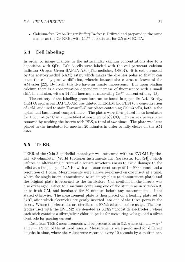
In order to image changes in the intracellular calcium concentrations due to adeposition with QDs, Calu-3 cells were labeled with the cell permeant calciumindicator Oregon Green BAPTA-AM (Thermofisher, O6807). It is cell permeantby the acetoxymethyl (-AM) ester, which makes the dye less polar so that it canenter the cell by passive diffusion, wherein intracellular esterases cleaves of theAM ester [22]. By itself, this dye have an innate fluorescence. But upon bindingcalcium there is a concentration dependent increase of fluorescence with a smallshift in emission, with a 14-fold increase at saturating Ca2+-concentrations, [23].

The entirety of the labelling procedure can be found in appendix A.4. Briefly,4mM Oregon green BAPTA-AM was diluted in EMEM (no FBS) to a concentrationof 4µM, and used to stain Transwell-Clear plates containing Calu-3 cells, both in theapical and basolateral compartments. The plates were then placed in an incubatorfor 1 hour at 37° C in a humidified atmosphere of 5% CO2. Excessive dye was laterremoved by washing the inserts with PBS, a total of two times. The plate was laterplaced in the incubator for another 20 minutes in order to fully cleave off the AMester.

5.5 TEER

TEER of the Calu-3 epithelial monolayer was measured with an EVOM2 Epithe-lial volt-ohmmeter (World Precision Instruments Inc, Sarasosta, FL, [24]), whichutilizes an alternating current of a square waveform (so as to avoid damage to thecells) at a frequency of 12.5 Hz with a measurement range of 1− 9999 ohms, and aresolution of 1 ohm. Measurements were always performed on one insert at a time,where the single insert is transferred to an empty plate (a measurement plate) andthe original plate is returned to the incubator. Cell medium in the inserts wasalso exchanged, either to a medium containing one of the stimuli as in section 5.3,or to fresh GM, and incubated for 30 minutes before any measurement - if notstated otherwise. The measurement plate is then placed on a heating plate set to37°C, after which electrodes are gently inserted into one of the three ports in theinsert. Where the electrodes are sterilized in 99.5% ethanol before usage. The elec-trodes used with the EVOM2 are denoted as STX2/"chopstick electrodes", whereeach stick contains a silver/silver-chloride pellet for measuring voltage and a silverelectrode for passing current.

Data from TEER measurements will be presented as in 3.2, whereMinsert = πr2

and r = 1.2 cm of the utilized inserts. Measurements were performed for differentlengths in time, where the values were recorded every 10 seconds by a multimeter.


5.6 Microscopy

Optical imaging of Calu-3 cells with the different stimuli as in 5.3, and the sub-sequent response to a deposition of QDs/ATP was performed using a LSM780confocal microscope (Carl Zeiss, Jena, Germany) equipped with a C-Apochromat40x/1.20 W korr FCS M27. Inserts labelled with Oregon green BAPTA-AM wereplaced on a 50mm diameter wide coverglass, and mounted in a stage-top incubatormaintained at a temperature of 37°C.

Excitation was achieved with an Argon multiline laser set to the wavelength of488nm. Emission from the Oregon Green BAPTA was detected with a 490-545 nmbandpass filter (green channel), and a 588-642 nm bandpass filter (red channel) wasused to detect emission from the QDs. Settings of the microscope, i.e. detector gain,amplifier offset, amplifier gain and size of pinhole, needed to be altered during allexperiments, depending on the stimuli in use, in order to achieve optimal imagingof the inserts. The laser transmission intensity of the 488 nm laser was howeveralways set to 3%.

The first imaging experiments was achieved by z-stack, times series mode, with30s intervals, for a total measurement time of 10 minutes. Each z-stack resultedin 20 images being recorded, with a plane spacing of 2.76 µm. This mode resultsin a clear trade-off between speed, accuracy, and resolution by the need to includethe whole cell (i.e. large z-stack) and at the same time being able to record theresponse (i.e. short time series). The optimal settings was determined empiricallythrough trial and error, which resulted in an increased speed by using an imagesize of 256 by 256 pixels (211.7 · 211.7 µm2), and by only using the green channelfor detection. By using both the green and red channel for detection resulted inalmost double the amount of time per z-stack, hence it was not possible to includethem both. The 3D image with both the red and green channels were also acquiredbefore and after dynamic imaging.

A modified z-stack time series mode were also utilized, where the recordinginterval was 10s for each z-stack, for a total measurement time of 10 minutes. Inthis modified version, I utilized a variable z-plane spacing, where the goal was torecord the whole cell during the 10s interval, with as many z-planes as possible.The z-plane spacing will thus be mentioned when this mode was used. A higherpixel count were made possible with these measurements: 512 by 512 pixels (212.3· 212.3 µm2), and also the utilization of both the red and green channel.

One of the profitable advantages when running the z-stack, time series modeis of course the possibility for imaging over entire cells, and not just a single focalplane, thus gaining the whole cell response. But, there may be loss of informationif the mechanism controlling the Ca2+ changes are too fast. For instance, as latershown in results from TEER measurements in Fig. 6.2, the drop in TEER by theQDs are almost instantaneous and quite short-lived. Another disadvantage is thatthe QD signal can not be detected at the same time as the Oregon green. Hence,imaging experiments was also done by time series mode with both the green andthe red channel, where a focal plane towards the apical side of the cells were chosen

5.7. DATA ANALYSIS 23

for the measurements. The different stimuli were used for these measurements inorder to make comparative studies as well, and frames were recorded at 5s intervals.This mode also yielded the possibility to use the higher pixel count: 512 by 512pixels (212.3 · 212.3 µm2). The 3D and Lambda mode images of both the red andgreen channels were also acquired before and after dynamic imaging.

In all modes of imaging measurements, cells were stimulated with a total volumeof 50µL QDs, where the specific time point will be indicated for each result.

5.7 Data analysis

The first step in the analysis is performed with the software Fiji [25], by whichregions of interest (ROIs, i.e cells) are chosen for analysis from the images producedin the microscopy experiments. The choice of ROI is based on a few criterion;

• Little to no movement during the imaging, indication that they are alive.Some morphological reorganization will occur, hence the area is chosen toaccommodate this.

• High brightness in the areas, indicating proficient labeling. But, not toobright since this would either indicate dead cells, or that the specific areahave saturated the detector. Both of which would mean that the region is ofno interest.

• When the above criteria are met, ROIs are compared with collected Brightfield images to make sure there is only one cell in the ROI.

When a suitable region of interest have been chosen, a circle is manually drawnaround each region with Fiji, where the size of circle is typically around 12·12 pixels(0.832µm2) for the images of 256·256 pixels, and 24·24 (0.422µm2) for the imagesof 512·512 pixel. Coordinates of each region is saved into an excel sheet as theleftmost x- and y-coordinate, height and width.

Analysis have also been done on the whole imaged area for some cases, the samegeneral procedure is followed as in the following sections, but the ROI is then thewhole imaged area.

5.7.1 Single cellThe specific analysis done for single cell analysis is later done with Matlab, whichrequires that the image stacks(.lsm files) that the microscope software produces issplit into individual images, done with ImageJ for instance. Images can then beloaded into Matlab as matrices of the arbitrary unit intensity, with the functionImg.m (appendix B.2). In order to separate the wanted information, i.e. the datawithin the ROIs, from everything else, the function Mesh.m in appendix B.3 is usedto mask the data outside of the ROIs with the coordinates from the first step, anexample of this can be seen in Fig. 5.1. Ten ROIs are used for the analysis process.


Figure 5.1: Example of an applied mesh. (a) Without applied mesh, (b) withapplied mesh.

Furthermore, the master script Brightness.m (appendix B.1) handles the anal-ysis by loading in the images with Img.m, and applying masks outside of the ROIswith Mesh.m according to the specified coordinates from the first step. The inten-sity values of each pixel is then recalculated into Gray values and added togetherin each ROI. The Gray values are stored either in single matrix if a time series isanalysed, or in a cell array if it is a z-stack time series - where the Gray values alsoare added in the z direction in order to extract the total readout from a single cell.The last step in the analysis is to normalize each ROI, by dividing with the Grayvalue at t=0. A statistical analysis is later done by calculating the mean and stan-dard deviation for all chosen ROIs, which yields the possibility to plot the signaldevelopment over time, with error bars corresponding to the standard deviation.

5.7.2 Relative ChangeFrom the gathered, data a second form of analysis can also performed, wherein alarger subset of ROIs are utilized. With the aim of visualizing the distribution ofthe relative changes in the signal before, and after the deposition of QDs. This isachieved by randomly choosing 50 ROIs (any number of ROIs are possible) fromeither a z-stack time series mode, or a time series measurement.

The master script Brightness.m is used as before for the single cell analysis,with the added functionality to calculate the relative change of the signal. Whichis done according to equation 5.1, where t is the time point of QD deposition, Gis the calculated Gray value at some time t, and ∆R is the wanted relative changevalue in %.

∆R = GtGt−1

(5.1)

5.7. DATA ANALYSIS 25

The script then sends the calculated values into the function RelChange.m (ap-pendix B.4) in order to plot the distribution of the relative changes in signal foreach wanted z-plane and ROI. For each z-plane, an actual image from the mea-surements are extracted at t=0 as a reference, on which every ROI will be drawnat the specified coordinates, and filled by a color according to a scale set by allthe calculated R values (colorbar scale set by the function in appendix B.6. Thefunction in appendix B.5) is used to do the plotting of the ROIs and filling themwith color.

Chapter 6

Results

6.1 TEER

Previous studies have shown that the deposition of QDs on Calu-3 cells culturedfor over 24 days induces a sharp drop in the TEER values [13], with a recovery overtime. The results shown here aims to corroborate the previous results, but also tofurther examine the response by the deposition of QDs. The TEER progressionover time have thus been detected for Calu-3 cells whilst they were subjected tothe listed stimuli in section 5.3, and subsequently exposed to a deposition of eitherQDs or ATP. In Fig. 6.1.a, results from six different Calu-3 cell-containing insertscultured for 14 days are shown, where the measurement time was 15 minutes and5µM QDs were deposited after 5 and 10 minutes. It is apparent that the multipledepositions only induces an observable response in the Nifedipine case, where theoverall response is highly unsteady, and the QDs seem to induces an transientincrease in TEER. The deposition of ATP does induce a sharp drop, with a smallrecovery over time as well. The TEER development over time for Calu-3 cellscultured as either LCC or AIC, for 8, 15 and 22 days can be also seen in Fig 6.1.bwhen the total measurement time was 10 minutes, and QDs were deposited after 3and 6 minutes.

Long-term culture results can be seen in Fig. 6.2 for cells cultured 23 days ormore, where Fig. 6.2.a shows that a stimulation with either QDs or ATP inducesthe expected sharp decrease in TEER. But also that the addition of BTP2 seemto inhibit the response to the QDs and ATP. The total measurement time was 20minutes, and QDs or ATP were deposited after 5 minutes. Furthermore, a secondset of long-term measurement results can be seen in Fig. 6.2.b when QD depositionsoccurred according to the red dashed lines. In this case, it seems as though theaddition of Nifedipine blocks the response to the QD stimulation to some extent,which is the opposite reaction in regards to 6.1.a. It can also be seen that multipledepositions of QDs induces the sharp decrease of TEER, with recovery over time,at both depositions. The third case shows the response when the cell medium

27

28 CHAPTER 6. RESULTS

Figure 6.1: TEER results from measurements on Calu-3 cells, where it is specifiedin the plot what stimuli was used. (a) Six different 14 day old inserts were measuredfor 15 minutes, and a deposition of QDs or ATP occurred at 5 and 10 minutes, (b)TEER development over time at different culture times of LCC and AIC cells, at8, 15 and 22 days, with a deposition of QDs after 3 and 6 minutes. The results areshown at an offset from each other for easier interpretation.

have been replaced with Cf-KRB, where the initial response is that of a very sharpdeclining TEER (when no incubation occurred after the medium change) towardsbaseline values when no cells are present (measured to be around 0.45kΩ · cm2),after which an incubation for 20 minutes lead to increased TEER, and a subsequentsharp decline once measurements started. The multiple depositions of QDs doesnot seem to have any large effect on TEER in this case.

Figure 6.2: TEER results from measurements on Calu-3 cells cultured 23 days ormore, where it is specified in the plot what stimuli was used. (a) 20 minute mea-surement with QDs deposited at 5 minutes, (b) 3 inserts of different measurementtimes and QD deposition at the indicated red dashed lines. The results are shownat an offset from each other for easier interpretation.

6.2. CALCIUM SIGNALLING BY QD DEPOSITION 29

6.2 Calcium signalling by QD deposition

To investigate the specific role of calcium after a deposition of QDs on Calu-3monolayers, cells cultured as LCC were stained with Oregon green BAPTA-AMand imaged as per the methodology in section 5.6. The results in Fig. 6.3.a showsthe time course development from a z-stack time series measurement when cellswere kept in GM, and 8µM QDs were deposited at 4 minutes. There is an evidentincrease in the Oregon green signal directly following the addition of the QDsinFig. 6.3.a, alongside a very sharp drop of the Bright field as well 6.3.b. This isalso easily seen visually in the overlay images of the Bright field+Oregon green, asseen in figures 6.3.c-e, where 6.3.c is taken 30 s before-, 6.3.d directly after-, and6.3.e. 30s after QD deposition.

0,8

1,0

1,2

1,4

(c) t=4.0 min

0 2 4 6 8 101,6

1,8

2,0

2,2

2,4

2,6(b) G

ray

valu

e

(a)z=13.8 µm

z=33.12 µm

(d) t=4.5 min

Ore

gon

gree

nBr

ight

fiel

d

Time [min]

z=23.04 µm

(e) t=5 min

Figure 6.3: Signal development plotted over time at six different z-positions onOregon green labelled Calu-3 cells, with a deposition of 8µM QDs at 4 minutes. 10minute measurement time with a z scaling of 2.760µm. Gray value developmentof (a) Oregon green signal,(b) Bright field. Where the arrows signify the increasein z-position. Images taken (c) 30 s before, (d) directly after, (e) 30s after QDdeposition.


The above shows the brute force method, i.e. the signal development of theentire imaged area, where no account is taken for dead cells or any inhomogeneityin the labelling. So, I next decided to analyse the data according to a single cellapproach, where the specific methodology can be found in section 5.7. For the insertyielding the results presented in Fig. 6.3, I ran a second 10 minute z-stack timeseries measurement directly after the first one - with a second 8µM QD depositionafter 2 minutes. Ten regions were then chosen from the first set of data, anddata processing was done on the same regions in both the first and the secondexperiment. In order to plot the data from the two experiments on the same graph,the data from the second experiment was normalized with respect to the first. Theresulting single cell development due to multiple QD depositions over an entire cellcan be seen in Fig. 6.4, where there the increase in the Ca2+ signal by the first QDdeposition is even clearer, and a slight increase by the second deposition as well.

Figure 6.4: Signal development due to multiple depositions of 8µM QDs at theindicated red dashed lines, on Oregon green labelled Calu-3 cells. Ten regions ofinterest were chosen and analysis were done as per the method in section 5.7, (a)Oregon green (b) Bright field where error bars correspond to the standard deviation,(c) image from the first measurement showing an area in the middle of the cells,where the ten regions have been encircled, with a scale bar of 50µm.

After the multiple depositions of QDs, imaging with both the red and greenchannel was utilized for a single z-stack in order to visualize whether or not theQDs accumulate or penetrate through the cells. In Fig. 6.5.a, an image from withinthe cells are shown, and Fig. 6.5.b show an image extracted from above the cells.These are clear indications that the QDs seem to accumulate on top of the cells,


with little to no penetration. Fig. 6.5.c show an enlarged image from the orthogonalz-y, also showing the clear division between the green and red channel.

Figure 6.5: Frames from a single z-stack after multiple QD depositions when boththe green and red channel was utilized so as to image both the Oregon green andQD at the same time. (a) image from a z-position within the cells, (b) image from az-position above the cells, (c) enlarged orthogonal z-y view from the z-stack. 50µmscale bars.

6.2.1 Inhibition of either release or influx of calciumIn order to further quantify the changes in the intracellular concentrations of cal-cium as a result of a deposition of QDs on Calu-3, the cellular access to calcium wasdecreased by various means in order to inhibit either the release or influx of Ca2+.Calu-3 cells cultured as LCC were labelled as before with Oregon green BAPTA-AM, and subsequently exposed either to; Ca-free medium (Cf-KRB); SOCE blockerBTP2; VGCC inhibitor Nifedipine. Baseline measurements without inhibitors werefirst done on cells kept in a Ca2+-rich medium (Cr-KRB), with a deposition of 5µMQDs at the indicated red dashed line in Fig. 6.6, achieved by time series mode(seesection 5.6) and data was analysed per the single cell analysis method. As before,it was observed that a QD deposition induces a rapid, immediate increase in theOregon green signal (Fig. 6.6.a). A decrease in the Bright field (Fig. 6.6.b) was alsoobserved in the same fashion as for the z-stack time series results. Simultaneously,the red channel was used to detect the QD emission, as seen in Fig. 6.6.c, where thesignal before the QD deposition is due to the tail of the Oregon Green fluorescence.A second area was later chosen from the same insert, and the same measurementswas run once more - with similar results, Fig. 6.6 d-e.


0,8

1,0

1,2

0,8

1,0

1,2

0 1 2 3 4 50

2

4

6

1 2 3 4 5

1,0

1,2

1,4

Ore

gon

gree

nBr

ight

fiel

dQ

uant

um d

ot

(a)

Area 1 Area 2

t=1'50''

Nor

mal

ized

gra

y va

lue (d)

t=1'50''

(b) (e)

Time [min] Time [min]

(c) (f)

Figure 6.6: Signal development due to a deposition of QDs on Oregon green labelledCalu-3 cells, with a deposition of 5µM QDs at the red dashed line. Ten regionsof interest were chosen and analysis was done as per the method in section 5.7.(a)-(c) results of Area 1, and (d)-(e) of Area 2, where error bars correspond to thestandard deviation. The small insets are images taken from the stacks at the notedtime points, with scale bar of 50µm.

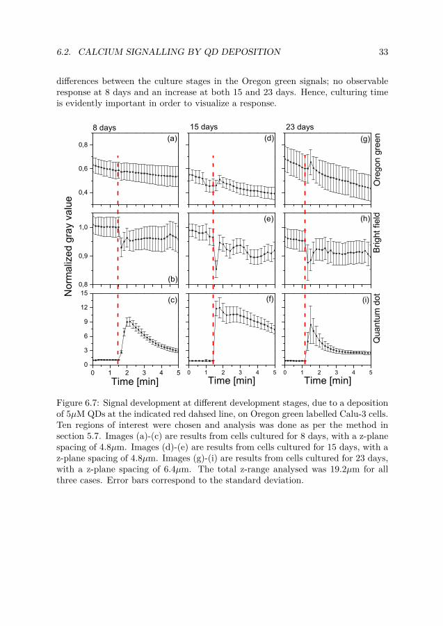
6.2.2 Time course developmentQuantification of the calcium signalling response, with respect to developmentphases were also measured for, with Calu-3 cells cultured using LCC for 8, 15or 23 days, and subsequently stained with Oregon Green as before. Measurementswere done per the modified z-stack time series mode, hence the z-scaling or totalz-distance is different for the three cases. Fig. 6.7 shows the results, when 5µmQDs were added after ca 6 minutes at the indicated red dahsed line, and the timescale have been shifted to 0 from the actual time of 5 min. The QD and Bright fieldshows the same general behaviour in all three instances, but there is however a clear


differences between the culture stages in the Oregon green signals; no observableresponse at 8 days and an increase at both 15 and 23 days. Hence, culturing timeis evidently important in order to visualize a response.

0,4

0,6

0,8

0,8

0,9

1,0

0 1 2 3 4 50

3

6

9

12

15

0 1 2 3 4 5 0 1 2 3 4 5

(b)

(c)

(a) (d) (g)

(h)(e)

(f) (i)

Time [min]Time [min]Time [min]

Nor

mal

ized

gra

y va

lue

8 days 15 days 23 days

Ore

gon

gree

nBr

ight

fiel

dQ

uant

um d

ot

Figure 6.7: Signal development at different development stages, due to a depositionof 5µM QDs at the indicated red dahsed line, on Oregon green labelled Calu-3 cells.Ten regions of interest were chosen and analysis was done as per the method insection 5.7. Images (a)-(c) are results from cells cultured for 8 days, with a z-planespacing of 4.8µm. Images (d)-(e) are results from cells cultured for 15 days, with az-plane spacing of 4.8µm. Images (g)-(i) are results from cells cultured for 23 days,with a z-plane spacing of 6.4µm. The total z-range analysed was 19.2µm for allthree cases. Error bars correspond to the standard deviation.


6.2.3 Inhibition measurementsFrom the TEER data, it is evident that experiments when Nifedipine was used,doesnot coincide with each other; at the young culture stage in Fig. 6.1.a, the TEERoscillate in a wavy fashion, with a transient increase by the QD stimulation; atthe late culture stage in Fig. 6.2.b, this wavy fashion is less pronounced, andthe deposition of QDs did not have a large effect on TEER. The other two calciumnegating casess are however aligned, in that both show no response to a stimulationwith the QDs.

The single cell response for the calcium negating stimuli were thus also measuredfor by imaging methods. When BTP2 and Ca-free medium was in use, the totalmeasurements were 5 minutes, with one frame recorded every 5s, and 5µM QDswas deposited after ca 1.5 minutes. Measurements of when Nifedipine was in usewere however done per the modified z-stack time series mode, with 1µM Nifedipineapplied to the growth medium. One z-stack was recorded every 10 seconds, witha total measurement time of 10 minutes, and 5µM QDs were deposited after ca 6minutes. Data analysis was done per the single cell analysis method in all threecases. The results can be seen in Fig. 6.8, wherein the sixth plane (z=24.45 µm) isshown from the Nifedipine measurement, and the time scale have been shifted tothe last 5 minutes (0-5 equals 5-10 in actual minutes)

It is evident from the BTP2 case in Fig. 6.8.a-c, that both the Bright field andQD signals are similar to the baseline Ca-rich result in Fig. 6.6. But, the blockingof the SOCE channels seem to inhibit the earlier observed increase of intracellularcalcium completely, as there is no observable change in the Oregon green signal.For the Ca-Free case in Fig. 6.8.d-f, there is also no observable increase in theOregon green signal, with a QD signal of the same behaviour as before. But, theredoes not seem to be any decrease in the Bright field signal however. The resultsfrom the Nifedipine measurements in Fig. 6.8.g-i, however shows a distinct increasein the Oregon green, and a decrease of the Bright field, just like when no inhibitoris present.


0,8

1,0

1,2

0,3

0,6

0,9

1,2

0,8

1,0

1,2

0,9

1,0

1,1

0 1 2 3 4 5

1

2

3

1 2 3 4 50

3

6

9

0,6

0,8

1,0

1,2

1,4

0,90

0,95

1,00

1,05

1,10

0 1 2 3 4 50

2

4

6

(a)Nif

Time [min]Time [min]Time [min]

Nor

mal

ized

Gra

y Va

lue

(d) (g)

(h)

(i)

(b) (e)

Ore

gon

Gre

enBr

ight

fiel

dQ

uant

um D

ot

(c)

t=1'50''

t=2'45''

(f)

Ca-freeBTP2

t=1'10''

Figure 6.8: Signal development due to a deposition of 5µM QDs at the red dashedline, on Oregon green labelled Calu-3 cells whilst access to calcium was inhibited.Ten regions of interest were chosen and analysis was done as per the method insection 5.7. Images (a)-(c) are results for when cells had been exposed to 50µMBTP2, (d)-(e) are results from when cells had been exposed to a Ca-Free (Cf-KRB) medium, and (g)-(i) are results from when cells had been exposed to a1µM Nifedipine. Error bars correspond to the standard deviation. BTP2 and Ca-free measurements were done by time series mode, with 5s intervals between eachrecorded frame. The Nifedipine results are from a z-stack time series measurement,with 10s intervals, where this plot shows the development from one z-plane at24.5µm. The insets correspond to a recorded image with the chosen ROIs encircledat the noted time, with scale bars of 50µm.

The same measurement method which yielded the previous Nifedipine result inFig. 6.8 were also done for an insert exposed to a Ca-rich medium, functioningas a control sample. The Oregon Green signal development from both of thesemeasurements can be seen in Fig. 6.9.a-b,when analysis is done on the wholeimaged area, and the time scale have been shifted to the last 5 minutes (0-5 equals


5-10 in actual minutes). The two results are similar, in that it seems as thoughthere is a decrease in the Gregon green signal towards the basolateral sides of theinserts, and an increase towards the apical side of the inserts.

In an attempt to further quantify this response, a normalization to one, andstatistical analysis yielding the mean and standard deviation was done - as seenin Fig 6.9.c-d. Showcasing that the statistical net change in signal is that of anincrease.

0

2

4

6

8

0 1 2 3 4 5

2

4

6

0,4

0,6

0,8

1,0

0 1 2 3 4 5

0,8

1,0

Time [min]

Gra

y va

lue

z=0-38.19 m(a)

(b) z=0-29.34 m

Nor

m. g

ray

valu

eTime [min]

Ca-

rich

Nif

(c)

(d)

Figure 6.9: Oregon Green signal development due a depositions of 5µM QDs atthe indicated red dashed line, on Oregon green labelled Calu-3 cells. (a) Cells inCa-rich medium with a z-plane spacing 6.4 µm, (b) Cells in Ca-rich medium and1µM Nifedipine, with a z-plane spacing 4.9 µm. (c) and (d) corresponds to thesame inserts as in (a) and (b) after normalization to 1 was done, and the shownplot is of the mean values for this time period, where error bars are of the standarddeviation.


6.2.4 Distriution of the individual cell responseThe results from Fig. 6.9 show distinct differences from previous results, wherein itindicates that the calcium response varies throughout the cell - whereas it seemedto be a relatively homogeneous increase in the results from figures 6.3 and 6.4. Inan effort to visualize the distribution of the individual cell response, 50 cells werechosen at random in the imaged area, and the relative signal change from beforeand after QD stimulation were calculated for each cell. The results can be seen inFig. 6.10, where the encircled spots corresponds to cells in the measured insert,and their color (see the colorbar in Fig. 6.10.h) indicates the relative change of theOregon green signal. It is evident from these results that there is a high variabilityin the single cell response.

(a) (b) (c)

(d) (e) (f)

1.50

1.36

1.22

1.08

0.94

0.80

(g)

(h)

Figure 6.10: Relative changes in the Oregon Green signal by 5µM deposition ofQDs, from a z-stack time series measurement, with a z-plane spacing of 6.4 µM.


6.3 AIC cultured Calu-3 cells

0,6

0,8

1,0

1,2

1,4

1,6

0,6

0,8

1,0

1,2

1,4

1,6

0,6

0,8

1,0

1,2

1,4

1,6

1 2 3 4 5

0,4

0,6

0,8

1,0

1,2

1,4

1,6

Nor

mal

ized

Gra

y Va

lue (a)

50 l Buffer

(e) 1'30'' (f) 2'

Time [min]

25nM QDs

(b)

0.25 M QDs

(c)

5 M QDs

(d)

Figure 6.11: Calcium signal and morphology ofCalu-3 cells cultured using AIC induced by QDstimulation. Cells were imaged for a total of 5minutes after staining. 50µL KRB buffer (a),25nM (b), 0.25µM(c) or 5µM (d) QDs were de-posited into the insert. Overlay images with Ore-gon green+Bright field are shown before (e) andafter (f) stimulation, and are placed to the right ofthe corresponding measurement with 10 µm scalebars

Calu-3 cells cultured using AICwas later imaged in order tocompare how different cultureconditions may affect the re-sponse to a deposition of QDs.The measurements were doneon four cell containing inserts,and QDs were deposited af-ter 100s. The total depositedliquid volume was in all fourcases 50µL, with an increasingconcentration of QDs for thefour depositions; 0M (i.e 50µLKRB buffer), 25nM, 0.25µMand 5µM. A compilation ofthe Oregon green signal de-velopment is shown in Fig.6.11 alongside images showcas-ing the morphology before andafter QD deposition. Mea-surements were done by timeseries mode, with one framerecorded every 5s, for a totalmeasurement time of 5 min.The deposition with 0M QDsdoes not induce any observablechanges, neither morphologi-cal nor changes in the Oregongreen, shown in Fig. 6.11.a andthe first two images of 6.11.e-f. The Oregon green signalfor the 25nM deposition havea constant upwards incline be-fore and after the deposition,6.11.b. But it seem to cause a great change in the overall morphology, where acomparison of the before and after images shows that cells are either moving closeror stacking onto neighbouring cells, second row of 6.11.e-f. A very large drop in theOregon green signal was observed for both the 0.25µM and 5µM cases, 6.11.c and6.11.d, with a large morphological change for the 0.25µM case as well (third row of6.11.e-f). Changes in morphology for the 5µM case is harder to distinguish though,it is possibly lost in its entirety due to cell death (fourth row of 6.11.e-f).

6.3. AIC CULTURED CALU-3 CELLS 39

6.3.1 LCC compared with AICFrom the recorded bright field images which yielded the previous results in Fig.6.11, it is evident that a higher QD concentration yields a larger morphologicalchange, possibly due to cell death. So as to compare the morphological changesinduced by a deposition of QDs, images have been extracted from z-stacks recordedbefore and after QD stimulation, for both LCC and AIC measurements. These arevizualised in Fig 6.12, where the extracted images are from a position within thecells at the indicated z position. For the LCC case (before: Fig. 6.12.a and after:6.12.b) a total of 16 µ M QDs were deposited onto the cells, showing little to nochange in the overall morphology. On the other hand, AIC cultured cells exposed toa total of 0.5µM QDs shows a very large change in the overall morphology (before:Fig. 6.12.c and after: 6.12.d).

z=16.56 m

(a)

(b)

(c)

(d)

z=16.56 m

z=16.56 m

z=18 m

z=18 m

Figure 6.12: Bright field images of Calu-3 cells cultured either using LCC or AICbefore and after a deposition of QDs. LCC; (a) Before QDs, (b) after 16 µM QDs.AIC; (c) Before QDs, (d) after 0.5µM QDs.

Chapter 7

Discussion

There are plenty of factors that may alter the functionality and modulate the respi-ratory barrier in a negative manor, such as a viral infection causing loss of integrityor a change in the morphology [26]. The junctioncal complexes play a major rolefor the overall functionality of this modulation. In previous work [13], TEER wasutilized in order to detect whether or not a deposition of QDs would affect the in-tegrity of the human airway epithelial Calu-3 cell monolayer, TEER measurementsrevealed a transient, sharp drop immediately following the deposition of QDs, witha recovery over time back to baseline values. Measurements were repeated over a sixday period without any obvious changes in either cell morphology, nor to baselineTEER values.

The results in this thesis shows that the deposition of QDs on Calu-3 epithelialcells cultured using LCC stimulates an instantaneous and transient increase ofintracellular calcium levels, shown for example in both Fig. 6.4 and 6.6. The effectof a second stimulation can also be seen in the same figures, where it is clear thatwhen the same set of cells are exposed to QDs the response is weaker in magnitude,but there is still a clear increase in the calcium signal. It is also evident from Fig.6.5 that the QDs does not penetrate the cell monolayer, therefore not inducing anymorphological damage. Calcium thus have an important role in the cell response toa stimulation with QDs, where the theorized underlying mechanism in the previouswork was that the QDs interacted with the cells through mechanical stimulation ofthe cilium.

The dominating route for Ca2+ signalling in non-excitable cells are by store-operated calcium channels, which functions as a two step process, [27]; first, by therelease of Ca2+ from the endoplasmic reticulum; second, the decreased ER Ca2+

content induces an influx of Ca2+ by channels present on the plasma membrane(store-operated Ca2+ entry or SOCE). In [27], it is stated that cell surface receptorsusually are present for activating this cascade, wherein the second messanger IP3is produced which then interacts with the ER for the release of Ca2+. Studieshave shown the role of the store-operated calcium channels and the importance of

41

42 CHAPTER 7. DISCUSSION

calcium with regards to ciliary beating, [28]. The SOCE inhibitor BTP2 was thusused to visualize any changes in the response to a stimulation of QDs in Calu-3cells. The results in Fig. 6.8.a clearly shows a total inhibition of the earlier observedcalcium increase without BTP2.

Due to the nature of TEER measurements, in that it is mainly the paracel-lular pathways that contributes to the results and that the observed response isinstantaneous for both TEER and calcium imaging. It is likely that the response ismediated through the paracellular pathway by altering the integrity of the mono-layer (i.e. drop in TEER). Modulation of the junctional complexes may thus bein a direct correlation with the re-distribution of calcium. In [29], the method ofFRET, amongst other methods, was used to show that cadherin molecules (of theadherens junctions) can alter their structural conformation in a short period of timeupon a change in the concentration of Ca2+. In another study [30], Calu-3 cellswere cultured on Transwell-Clear inserts to maturity, and when they were exposedto calcium free medium both in the apical and basolateral compartments, there wasa transient decrease of TEER and permeability. An increase in TEER was laterobserved when a calcium containing medium was reintroduced to the cells. In thisthesis, similar results were obtained at both an early stage in Fig. 6.1, and at alate culture stage in Fig. 6.2, wherein the Ca-free medium immediately caused adecrease in TEER. The deposition of QDs yielded no observable response as well.Imaging of Calu-3 cells when using a Ca-free medium also yielded no observableresponse to the deposition of QDs, Fig. 6.8.b. This result, together with the showninhibition of calcium increase when BTP2 is present in the cell medium, impliesthe importance of access to calcium during the response of airway epithelial cellsto a simulation with QDs.

Calcium entry into cells can also be mediated by voltage-gated Ca2+ channels,wherein it acts as a second messenger for electrical signalling, and can thus initiatecellular events such as contraction, secretion and neurotransmission [31]. Suchinflux of calcium is achieved in response to action potentials and depolarizing signalswhich in both cases have caused the membrane to depolarize [32]. Nifedipine wasthus used in order to block these forms of channels, and when it was first used forthe early stage TEER measurements (Fig. 6.1.a) the shown behaviour is highlyunsteady, and it seems as if there is an increase in TEER after QDs were deposited.At the late culture stage though, TEER shows very little response to the QDs inFig. 6.2.b, a small decline is however seen in the TEER after the second deposition.The imaging results from both Fig. 6.9, and Fig. 6.8 clearly shows that the Oregongreen signal actually increases for some z-planes when the QDs stimulate the cells.Hence, there are clear indications of Nifedipine not being able to block the responseto the QD deposition, and not contributing to the overall observed response.

There is some divergence in the reported results in this thesis, the first imagingresults of the z-stack time measurements in Fig. 6.3 and Fig. 6.4 clearly indicatesthat the Oregon green signal response is the same throughout the cell, when arecording interval for one z-stack is 30s. But, later measurements with the mod-ified z-stack time measurements such as in Fig. 6.9, where a much shorter time

43

interval is used (10s), indicates that the response varies - by a decrease in [Ca2+]itowards the basolateral side of the inserts, and increasing towards the apical side.Which probably is more of the true response, due to the theorized interaction isby mechanical stimulation of the primary-cilia located extracellularly on the apicalside. The 30s interval time in the first measurements are thus probably to slow tocatch the actual transient response, it only catches the end result. The analysisdone in Fig 6.10 paves further evidence for this idea. Furthermore, the normalizedgraphs in Fig. 6.9.c-d shows that the overall net response is that of an increasedintracellular calcium concentration in the cells.

Tight junctions regulate paracellular permeability, and are thus highly impor-tant for the respiratory barrier. But, the functionality is very complex due to therebeing over 50 proteins associated to TJs, such as the transmembrane proteins junc-tional adhesion molecule (JAM), occludin, and claudin. They also interconnectand interact with cytoskeletal structures, including actin microfilaments and mi-crotubules located on the intracellular side of the plasma membrane. Interactionswhich occurs via scaffolding proteins zonula occludens ZO-1, ZO-2, and ZO-3 whichall contain PDZ-domains (post synaptic density protein, Drosophila disc large tu-mor suppressor, and ZO-1). Studies indicate that cytoplasmic interactions playsa large role in both remodulation and alteration of both TJ structure and perme-ability, such as in [33] where it is shown that it may depend on phosphorylationpatterns of cytoskeletal proteins. Further evidence for the modulation of TJs viainteraction with the cytoskeleton can be found in the work done by Stefano Castel-lani et al. in [34]. Where an overexpression of the CTFR and Na+/H+ ExchangeRegulatory Factor (NHERF1, which most often is found apically in polarized cells)in human bronchial epithelial airway cells lead to a re-organisation of TJs and areduced permeability to small solutes. Hence, the underlying mechanism behindthe observed increased intracellular calcium levels in this thesis probably occursvia signalling cascades which simply starts with the mechanical stimulation by theQDs.

An investigation into different culture methodology were also done in this thesis,in an effort to compare the cell response for Calu-3 cells cultured either using LCC orAIC. TEER values were firstly much lower in the AIC case compared to LCC, whichis corroborated by previous studies [35]. There were also no observed response tothe deposition of QDs during the TEER measurements in the AIC case. Imaging ofthe AIC cells did however yield interesting results, such as a major decrease in theOregon green signal for high concentration of the deposited QDs - Fig. 6.11. But,upon closer inspection of the Bright field images, it was evident that the observedchange in calcium was more likely due to a morphology change. A morphologychange which is hard to characterize from the images, cells exhibiting a strong signalcould for instance have been covered by other cells, or by actual cell deformation.In the third row of Fig. 6.11.e-f, arrows are drawn on the images to show howthe center of the cells moves in position after the QD deposition. The Bright fieldimages in Fig. 6.12 also clearly shows how the morphology change before, and afterQD deposition differs between the AIC and LCC cultured methods.

Chapter 8

Conclusion

From the presented results in this thesis, it is plausible to say that a deposition ofQDs on Human airway epithelial Calu-3 cultured using LCC induces an increase ofthe intracellular calcium levels. The response was not observed at an early culturestage, hence there is a need for cell maturity in order to exhibit this mechanism.This increase seem to be mediated without voltage gated calcium channels, as itstill was observed when a inhibitor of the VGCC was used. However, it was totallyblocked when a inhibitor of the store-operated calcium entry was used, and alsowhen calcium was removed from the cell medium. The exact signalling cascadethat still needs to be answered through.

The observed decrease in TEER suggests that cells loose integrity, and are lesstightly bound to neighbouring cells, but there is virtually no penetration of QDsthrough the epithelial monolayers, Fig. 6.5. The increase of intracellular calciumcould be then be induced as some form of a defensive mechanism, which takesdifferent forms depending on the culture method.

45

Bibliography

[1] A. Elsaesser and C. V. Howard, “Toxicology of nanoparticles,” AdvancedDrug Delivery Reviews, vol. 64, no. 2, pp. 129–137, Feb. 2012, DOI:10.1016/j.addr.2011.09.001.

[2] L. Yildirimer, N. T. Thanh, M. Loizidou, and A. M. Seifalian, “Toxicologyand clinical potential of nanoparticles,” Nano Today, vol. 6, no. 6, pp.585–607, Dec. 2011, DOI: 10.1016/j.nantod.2011.10.001.

[3] R. Vogelmann and W. J. Nelson, “Fractionation of the Epithelial ApicalJunctional Complex: Reassessment of Protein Distributions in DifferentSubstructures,” Molecular Biology of the Cell, vol. 16, no. 2, pp. 701–716,Feb. 2005, DOI: 10.1091/mbc.E04-09-0827.

[4] S. Tsukita, M. Furuse, and M. Itoh, “Multifunctional strands in tightjunctions,” Nature Reviews Molecular Cell Biology, vol. 2, no. 4, pp. 285–293,Apr. 2001, DOI: 10.1038/35067088.

[5] K. A. Min, G. R. Rosania, C.-K. Kim, and M. C. Shin, “Functional andcytometric examination of different human lung epithelial cell types as drugtransport barriers,” Archives of Pharmacal Research, vol. 39, no. 3, pp.359–369, Jan. 2016, DOI: 10.1007/s12272-015-0704-6.

[6] H. M. Braakhuis, S. K. Kloet, S. Kezic, F. Kuper, M. V. D. Z. Park,S. Bellmann, M. van der Zande, S. Le Gac, P. Krystek, R. J. B. Peters, I. M.C. M. Rietjens, and H. Bouwmeester, “Progress and future of in vitro modelsto study translocation of nanoparticles,” Archives of Toxicology, vol. 89,no. 9, pp. 1469–1495, Sep. 2015, DOI: 10.1007/s00204-015-1518-5.

[7] B. I. Florea, M. L. Cassara, H. E. Junginger, and G. Borchard, “Drugtransport and metabolism characteristics of the human airway epithelial cellline Calu-3,” Journal of Controlled Release, vol. 87, no. 1–3, pp. 131–138,Feb. 2003, DOI: 10.1016/S0168-3659(02)00356-5.

[8] M. Marušić, I. Djurdjevič, K. Drašlar, and S. Caserman, “Calu-3 modelunder AIC and LCC conditions and application for protein permeabilitystudies,” Acta Chimica Slovenica, vol. 61, no. 1, pp. 100–109, 2014.

47

http://dx.doi.org/10.1016/j.addr.2011.09.001

http://dx.doi.org/10.1016/j.nantod.2011.10.001

http://dx.doi.org/10.1091/mbc.E04-09-0827

http://dx.doi.org/10.1038/35067088

http://dx.doi.org/10.1007/s12272-015-0704-6

http://dx.doi.org/10.1007/s00204-015-1518-5

http://dx.doi.org/10.1016/S0168-3659(02)00356-5

48 BIBLIOGRAPHY

[9] J. Shan, J. Huang, J. Liao, R. Robert, and J. W. Hanrahan, “Anion secretionby a model epithelium: more lessons from Calu-3,” Acta Physiologica, vol.202, no. 3, pp. 523–531, Jul. 2011, DOI: 10.1111/j.1748-1716.2011.02253.x.

[10] A. Banga, F. A. Witzmann, H. I. Petrache, and B. L. Blazer-Yost,“Functional effects of nanoparticle exposure on Calu-3 airway epithelialcells,” Cellular Physiology and Biochemistry: International Journal ofExperimental Cellular Physiology, Biochemistry, and Pharmacology, vol. 29,no. 1-2, pp. 197–212, 2012, DOI: 10.1159/000337601.

[11] A. Sekiyama, Y. Gon, M. Terakado, I. Takeshita, Y. Kozu, S. Maruoka,K. Matsumoto, and S. Hashimoto, “Glucocorticoids enhance airway epithelialbarrier integrity,” International Immunopharmacology, vol. 12, no. 2, pp.350–357, Feb. 2012, DOI: 10.1016/j.intimp.2011.12.006.

[12] I. George, G. Naudin, S. Boland, S. Mornet, V. Contremoulins, K. Beugnon,L. Martinon, O. Lambert, and A. Baeza-Squiban, “Metallic oxidenanoparticle translocation across the human bronchial epithelial barrier,”Nanoscale, vol. 7, no. 10, pp. 4529–4544, 2015, DOI: 10.1039/C4NR07079H.

[13] A. Turdalieva, J. Solandt, N. Shambetova, H. Xu, H. Blom, H. Brismar,M. Zelenina, and Y. Fu, “Bioelectric and Morphological Response ofLiquid-Covered Human Airway Epithelial Calu-3 Cell Monolayer to PeriodicDeposition of Colloidal 3-Mercaptopropionic-Acid Coated CdSe-CdS/ZnSCore-Multishell Quantum Dots,” PLoS ONE, vol. 11, no. 2, Feb. 2016, DOI:10.1371/journal.pone.0149915.

[14] B. Nicholas, P. Skipp, R. Mould, S. Rennard, D. E. Davies, C. D. O’Connor,and R. Djukanović, “Shotgun proteomic analysis of human-induced sputum,”PROTEOMICS, vol. 6, no. 15, pp. 4390–4401, Aug. 2006, DOI:10.1002/pmic.200600011.

[15] K. R. Spring, “Routes and Mechanism of Fluid Transport by Epithelia,”Annual Review of Physiology, vol. 60, no. 1, pp. 105–119, 1998, DOI:10.1146/annurev.physiol.60.1.105.

[16] C. Kittel, Introduction to Solid State Physics, eigth ed. Wiley, 1996. ISBN978-0-471-41526-8

[17] Y. Fu and K. A. Chao, “Validity of the third-derivative modulationspectroscopy,” Physical Review B, vol. 40, no. 16, pp. 10 712–10 716, Dec.1989, DOI: 10.1103/PhysRevB.40.10712.

[18] Y. Fu, Physical Models of Semiconductor Quantum Devices, 2nd ed.Springer, 2013. ISBN 978-94-007-7173-4

http://dx.doi.org/10.1111/j.1748-1716.2011.02253.x

http://dx.doi.org/10.1159/000337601

http://dx.doi.org/10.1016/j.intimp.2011.12.006

http://dx.doi.org/10.1039/C4NR07079H

http://dx.doi.org/10.1371/journal.pone.0149915

http://dx.doi.org/10.1002/pmic.200600011

http://dx.doi.org/10.1146/annurev.physiol.60.1.105

http://dx.doi.org/10.1103/PhysRevB.40.10712

BIBLIOGRAPHY 49

[19] L. Brus, “Electronic wave functions in semiconductor clusters: experimentand theory,” The Journal of Physical Chemistry, vol. 90, no. 12, pp.2555–2560, Jun. 1986, DOI: 10.1021/j100403a003.

[20] J. L. Harcourt and L. M. Haynes, “Establishing a liquid-covered culture ofpolarized human airway epithelial Calu-3 cells to study host cell response torespiratory pathogens in vitro,” Journal of Visualized Experiments: JoVE,no. 72, 2013, DOI: 10.3791/50157.

[21] L. Li, G. Tian, Y. Luo, H. Brismar, and Y. Fu, “Blinking, Flickering, andCorrelation in Fluorescence of Single Colloidal CdSe Quantum Dots withDifferent Shells under Different Excitations,” The Journal of PhysicalChemistry C, vol. 117, no. 9, pp. 4844–4851, Mar. 2013, DOI:10.1021/jp311975h.

[22] J. R. Lakowicz, Principles of Fluorescence Spectroscopy, 3rd ed. Springer,2006. ISBN 978-0-387-31278-1

[23] Invitrogen, “Long-Wavelength Calcium Indicators,” 2008. [Online]. Available:https://tools.thermofisher.com/content/sfs/manuals/mp03010.pdf

[24] World Precision Instruments Inc, “Epithelial Voltohmmeter,” [Accessed14-March-2016]. [Online]. Available: http://www.wpi-europe.com/products/cell-and-tissue/teer-measurement/evom2.aspx

[25] J. Schindelin, I. Arganda-Carreras, E. Frise, V. Kaynig, M. Longair,T. Pietzsch, S. Preibisch, C. Rueden, S. Saalfeld, B. Schmid, J.-Y. Tinevez,D. J. White, V. Hartenstein, K. Eliceiri, P. Tomancak, and A. Cardona,“Fiji: an open-source platform for biological-image analysis,” NatureMethods, vol. 9, no. 7, pp. 676–682, Jul. 2012, DOI: 10.1038/nmeth.2019.

[26] M. Vareille, E. Kieninger, M. R. Edwards, and N. Regamey, “The airwayepithelium: soldier in the fight against respiratory viruses,” ClinicalMicrobiology Reviews, vol. 24, no. 1, pp. 210–229, Jan. 2011, DOI:10.1128/CMR.00014-10.

[27] J. T. Smyth, S.-Y. Hwang, T. Tomita, W. I. DeHaven, J. C. Mercer, andJ. W. Putney, “Activation and regulation of store-operated calcium entry,”Journal of Cellular and Molecular Medicine, vol. 14, no. 10, pp. 2337–2349,Oct. 2010, DOI: 10.1111/j.1582-4934.2010.01168.x. [Online]. Available:http://www.ncbi.nlm.nih.gov/pmc/articles/PMC3074973/

[28] A. Schmid and M. Salathe, “Ciliary beat co-ordination by calcium,” Biologyof the Cell / Under the Auspices of the European Cell Biology Organization,vol. 103, no. 4, pp. 159–169, Apr. 2011, DOI: 10.1042/BC20100120.

http://dx.doi.org/10.1021/j100403a003

http://dx.doi.org/10.3791/50157

http://dx.doi.org/10.1021/jp311975h

https://tools.thermofisher.com/content/sfs/manuals/mp03010.pdf

http://www.wpi-europe.com/products/cell-and-tissue/teer-measurement/evom2.aspx

http://www.wpi-europe.com/products/cell-and-tissue/teer-measurement/evom2.aspx

http://dx.doi.org/10.1038/nmeth.2019

http://dx.doi.org/10.1128/CMR.00014-10

http://dx.doi.org/10.1111/j.1582-4934.2010.01168.x

http://www.ncbi.nlm.nih.gov/pmc/articles/PMC3074973/

http://dx.doi.org/10.1042/BC20100120

50 BIBLIOGRAPHY

[29] S. A. Kim, C.-Y. Tai, L.-P. Mok, E. A. Mosser, and E. M. Schuman,“Calcium-dependent dynamics of cadherin interactions at cell–cell junctions,”Proceedings of the National Academy of Sciences, vol. 108, no. 24, pp.9857–9862, Jun. 2011, DOI: 10.1073/pnas.1019003108.

[30] D. Vllasaliu, S. Shubber, M. Garnett, C. Alexander, M. Eaton, andS. Stolnik, “Evaluation of calcium depletion as a strategy for enhancement ofmucosal absorption of macromolecules,” Biochemical and BiophysicalResearch Communications, vol. 418, no. 1, pp. 128–133, Feb. 2012, DOI:10.1016/j.bbrc.2011.12.146.

[31] F. H. Yu and W. A. Catterall, “The VGL-Chanome: A Protein SuperfamilySpecialized for Electrical Signaling and Ionic Homeostasis,” Sci. STKE, vol.2004, no. 253, p. re15, Oct. 2004, DOI: 10.1126/stke.2532004re15. [Online].Available: http://stke.sciencemag.org/content/2004/253/re15

[32] W. A. Catterall, “Voltage-Gated Calcium Channels,” Cold Spring HarborPerspectives in Biology, vol. 3, no. 8, p. a003947, Aug. 2011, DOI:10.1101/cshperspect.a003947. [Online]. Available:http://cshperspectives.cshlp.org/content/3/8/a003947

[33] J. Miyoshi and Y. Takai, “Structural and functional associations of apicaljunctions with cytoskeleton,” Biochimica Et Biophysica Acta, vol. 1778,no. 3, pp. 670–691, Mar. 2008, DOI: 10.1016/j.bbamem.2007.12.014.

[34] S. Castellani, L. Guerra, M. Favia, S. Di Gioia, V. Casavola, and M. Conese,“NHERF1 and CFTR restore tight junction organisation and function incystic fibrosis airway epithelial cells: role of ezrin and the RhoA/ROCKpathway,” Laboratory Investigation; a Journal of Technical Methods andPathology, vol. 92, no. 11, pp. 1527–1540, Nov. 2012, DOI:10.1038/labinvest.2012.123.

[35] A. Stentebjerg-Andersen, I. V. Notlevsen, B. Brodin, and C. U. Nielsen,“Calu-3 cells grown under AIC and LCC conditions: Implications fordipeptide uptake and transepithelial transport of substances,” EuropeanJournal of Pharmaceutics and Biopharmaceutics, vol. 78, no. 1, pp. 19–26,May 2011, DOI: 10.1016/j.ejpb.2010.12.030. [Online]. Available:http://www.sciencedirect.com/science/article/pii/S0939641110003711

http://dx.doi.org/10.1073/pnas.1019003108

http://dx.doi.org/10.1016/j.bbrc.2011.12.146

http://dx.doi.org/10.1126/stke.2532004re15

http://stke.sciencemag.org/content/2004/253/re15

http://dx.doi.org/10.1101/cshperspect.a003947

http://cshperspectives.cshlp.org/content/3/8/a003947

http://dx.doi.org/10.1016/j.bbamem.2007.12.014

http://dx.doi.org/10.1038/labinvest.2012.123

http://dx.doi.org/10.1016/j.ejpb.2010.12.030

http://www.sciencedirect.com/science/article/pii/S0939641110003711

Appendix A

Calu-3: Culture and labeling

A.1 Introduction

General culturing guidelines for Calu-3 cells have previously been reported in [20]and closely resembles how the culturing was done for this report - with some alter-ations. Below in section A.3, is a step-by-step of how the Calu-3 cells were culturedfrom frozen storage until seeded into Transwell-Clear inserts.

During the confocal imaging experiments the Calu-3 cells were labeled withOregon Green Bapta AM. This dye have innate fluorescence on its own, but upon asaturating Ca2+-concentration there is a 14-fold increase in fluorescence [23]. Thelabeling procedure can be found in section A.4

A.2 Growth Medium

The growth medium utilized for Calu-3 cells contains Eagle’s Minimum EssentialMedium (EMEM) modified to contain 2mM L-glutamine, 1mM sodium pyruvate,and 1500mg/L sodium bicarbonate supplemented with 10% fetal bovine serum(FBS) and 100 units/ml of penicillin and 100µg/mL streptomyocin (P/S).

Before growth medium is added to the Calu-3 cells, it is always prewarmed ina heat bath set to 37°C for approximately 5 minutes.

A.3 Culture

The Calu-3 cells are so called immortalized cell lines originating from a patientwith bronchial adenocarcinoma. These are frozen under liquid nitrogen vapor phaseconditions in a cryovial supplemented with complete growth medium and 5% DMSOyielding a total volume of 1ml. Hence, the starting point is to thaw the cells.

• Thaw a cryovial of Calu-3 cells in a heath bath at 37°C by gently moving thevial in the bath until there are no visible ice crystals left in the liquid.

51

52 APPENDIX A. CALU-3: CULTURE AND LABELING

• Aspirate contents from the vial by pipette and transfer to a sterile tube con-taining growth medium at a 1:9 ratio and centrifuge for 5 minutes at 1400RPM.

Centrifugation accomplishes aggregation of the cells in the form of a pellet inthe bottom of the tube and it is done so as to separate the cells from the addedDMSO (if this is not removed the cells will not grow once thawed).

• Decant supernatant and resuspend cells with 5ml growth medium by gentlypipetting the liquid up and down. After complete resuspension, transfer thecontents from the tube to a petri dish.

• Wash tube with another 5ml growth medium and transfer to the same petridish.

• Place petri dish in an incubator at 37°C and 5% CO2

Cells will then, hopefully, grow, divide and thrive in the incubator, adheringto the petri dish and eventually reach confluency. Cells should, however not reacha confluency above 90% since this reduces the generation of polarized cultures -between 75-90% is optimal, according to [20]. The petri dish can be placed undera light microscope for a visual approximation of the confluency.

• Every 2-3 days, aspirate medium and wash with PBS and add 10ml growthmedium to the petri dish.

Growth medium will over time, loose its potency due to the cells ’using up’all the nutrients and thus it needs to be exchanged. How often medium need beexchanged depends on cell density, and the color of the medium essentially signifieswhen it is time to exchange it (when color changes from red to see-through, it needsto be exchanged).

When a confluency of 70-80% have been reached, the next stage of subculturinginto Transwell-Clear inserts can start.

• Remove petri dish from incubator. Aspirate old medium and wash twice with10ml PBS.

• Add 1ml of trypsin-EDTA and gently stir the petri dish. Aspirate by pipetteand discard.

• Add 3ml trypsin-EDTA and place petri dish in incubator at 37°C for 3 min-utes.

The trypsin-EDTA is added to dissociate the adherent cells from the petri dish.When added, it breaks down the proteins that enables the Calu-3 cells to adhereto the petri dish.

A.4. OREGON GREEN BAPTA-AM LABELING 53

• Remove petri dish from incubator and aspirate all its contents. Transfer toappropriate sterile tube and add equal amounts of growth medium as amountsof Trypsin were added the second time. Remove ca 30µl from tube and countcells with a haemocytometer.

• Centrifuge tube for 5 minutes at 1400 RPM. Decant supernatant and re-suspend cells in prewarmed growth medium. The amount of growth mediumdepends on the cell count, if the end goal is to seed cells into a Transwell-Clearplate it need to contain 5 ∗ 106 cells/ml.

• When resuspension is complete, seed 1ml of the cell containing liquid into eachof the six apical compartments of Transwell-Clear inserts at a density of 0.4 ∗106 cells/insert. Add 2ml growth medium to the basolateral compartments.Place the plate in an incubator at 37°C and 5% CO2

• Exchange growth medium every two days, both in the apical compartmentand in the basolateral compartment.

A.4 Oregon Green BAPTA-AM Labeling

From vials containing 50µg/vial Oregon Green, a stock solution is first prepared:

• Prepare Pluoronic Solution by dissolving 200mg Pluronic into 1mL DMSO.

• Add 10µL Pluronic solution into the Oregon Green vial to get 4mM OregonGreen stock solution

The stock solution should be covered by aluminum foil as well to minimize lightexposure. With the stock solution ready, the cells can be labeled.

• Prepare work solution by adding 1µL Oregon Green stock solution into 1mLEMEM. A total of 4mL work solution is needed.

• Add 1.5mL work solution into the insert compartment and 2.5mL into thebasolateral compartment. Incubate for 60 minutes at 37 °C and 5% CO2.

• Aspirate work solution, both from insert and basolateral compartment. Washwith PBS. Add 1mL growth medium to the insert and 2mL into the basolat-eral compartment. Incubate 20 minutes so that Oregon-Green Bapta AM iscleaved into Oregon-Green Bapta.

Appendix B

Sample Matlab code

B.1 Brightness.m

1 % Script for converting intensity in z−stack time series to Brightness2 % Export file series from ZEN 2012: file>export>3 % Format JPEG4 % Name as below;5 % Fluorescent is C16 % Brightfield is C27 % Second fluorescent channel is C38 % Data Raw data − series9 % comression ratio − 100

1011 clear all12 warning off MATLAB:imagesci:jpg:libraryMessage1314 % Construct a questdlg with three options15 choice = questdlg('What form of analysis would you like to do?', ...16 'Brightness.m', ...17 'Entire imaged area','Single cell','Relative change',...18 'Relative change');19 % Handle response20 switch choice21 case 'Entire imaged area'22 disp([choice ' analysis coming right up.'])23 choice = 1;24 case 'Single cell'25 disp([choice ' analysis coming right up.'])26 choice = 2;27 case 'Relative change'28 disp('Relative change analysis coming right up.')29 choice = 3;30 end31 if choice == 132 choice2 = questdlg('More than one z−plane?', ...33 'Planes', ...

55

56 APPENDIX B. SAMPLE MATLAB CODE

34 'Yes','No','No');35 switch choice236 case 'Yes'37 disp('Several plane analysis.')38 choice2 = 1;39 case 'No'40 disp('Single plane analysis.')41 choice2 = 2;42 end43 if choice2==144 prompt = 'Enter first Z−plane:',...45 'Enter last Z−plane:',...46 'Enter amount of cycles:',...47 'Enter amount of channels to be analyzed:',...48 'Enter interval time in time−series:';49 dlg_title = 'Single−cell analysis';50 defaultans = '1','2','60','2','10'; %Example values51 num_lines = 1;52 answer = inputdlg(prompt,dlg_title,num_lines,defaultans);5354 % Storing answers55 Zrange=str2double(answer1):str2double(answer2);56 cycles=str2double(answer3);57 channels=str2double(answer4);58 t_series_length=str2double(answer5);59 end60 if choice2==261 prompt = 'Enter amount of cycles:',...62 'Enter amount of channels to be analysed:',...63 'Enter interval time in time−series:'...64 'If applicable, enter z−plane to be analysed';65 dlg_title = 'Single−cell analysis';66 num_lines = 1;67 defaultans = '60','2','10','1'; %Example values6869 answer = inputdlg(prompt,dlg_title,num_lines,defaultans);70 % Storing answers71 cycles=str2double(answer1);72 channels=str2double(answer2);73 t_series_length=str2double(answer3);74 Zrange=str2double(answer4):str2double(answer4);75 end76 M=Zrange;77 end78 if choice == 2 || choice ==379 if choice ==280 prompt = 'Enter first Z−plane:',...81 'Enter last Z−plane:',...82 'Enter amount of cycles:',...83 'Enter amount of channels to be analyzed:',...84 'Enter interval time in time−series:';85 dlg_title = 'Single−cell analysis';86 defaultans = '1','2','60','2','10'; %Example values87 num_lines = 1;88 answer = inputdlg(prompt,dlg_title,num_lines,defaultans);

B.1. BRIGHTNESS.M 57

8990 % Storing answers91 Zrange=str2double(answer1):str2double(answer2);92 cycles=str2double(answer3);93 channels=str2double(answer4);94 t_series_length=str2double(answer5);95 end96 if choice == 397 prompt = 'Enter first Z−plane:',...98 'Enter last Z−plane:',...99 'Enter amount of cycles:',...

100 'Enter interval time in time−series:',...101 'Enter cycle of QD drop';102 dlg_title = 'Relative change';103 defaultans = '1','5','60','10','40'; %Example values104 num_lines = 1;105 answer = inputdlg(prompt,dlg_title,num_lines,defaultans);106 % Storing answers107 Zrange=str2double(answer1):str2double(answer2);108 cycles=str2double(answer3);109 t_series_length=str2double(answer4);110 t1=str2double(answer5)−2;111 t2=str2double(answer5)−1;112 channels=1;113 end114115116 % Read in Mesh data, should be named Mesh and be of format xlsx,117 % otherwis choose file118 try119 p = xlsread('MeshShort.xlsx');120 catch ME121 switch ME.identifier122 case 'MATLAB:xlsread:FileNotFound'123 warning('File of that name not found, choose');124 FileName=uigetfile('*.xlsx','Select mesh file');125 p = xlsread(FileName);126 otherwise127 return128 end129 end130131 %Calling mesh function132 M=Mesh(p);133 end134 Max = (channels*cycles*(length(Zrange))*length(M));135 h = waitbar(0,['Step 1 of ' num2str(Max)],'Name','Please wait...',...136 'CreateCancelBtn',...137 'setappdata(gcbf,''canceling'',1)');138 setappdata(h,'canceling',0)139 % Calling Img.m function to load images140 Im=Img(Zrange,cycles,channels);141142 % Placeholder for results143 for ch=1:channels


144 C.(sprintf('C%d',ch))=cell(1,length(M));145 su.(sprintf('suC%d',ch))=zeros(cycles,length(M));146 N.(sprintf('NC%d',ch))=zeros(cycles,length(M));147 end148149150 % Step counter151 s=0;152 if length(Zrange) == 1153 Zrange=1:1;154 end155156 % Run analyzis over the amount of channels, for the specified z planes157 % and for the amount of ROIs in the mesh158 for c=1:channels159 for k=Zrange160 for r=1:length(M)161 % Placeholder for image162 p_image=[];163 % Placeholder for results of analysis164 r_image=zeros(1,cycles);165 % Run calculation for the time series166 for m=1:cycles167 % Check for Cancel button press168 if getappdata(h,'canceling')169 delete(h)170 error('Stopped analysis')171 end172 % Steps173 s=s+1;174 waitbar(s/Max,...175 h,[sprintf('Step %d of ',s) num2str(Max)])176 image = Im.(sprintf('images%d',c))k,m;177178 % Apply mesh to data179 if ~choice==1180 image(Mr == 0) = 0;181 end182183 if choice == 1184 p(r,1)=1; p(r,2)=1;185 p(r,3)=length(image)−1;186 p(r,4)=length(image)−1;187 end188189 % Convert data to double190 p_image=im2double(image);191 Br=0.0;192193 for i=(p(r,2)):(p(r,2)+p(r,4));194 for j=(p(r,1)):(p(r,1)+p(r,3));195 % If 0 is used as a coordinate in the mesh196 if (i < 1), i=1;end197 if (j < 1), j=1;end198

B.1. BRIGHTNESS.M 59

199 % Brightness calculation for each pixel200 Br=0.2126*p_image(i,j,1)...201 +0.7152*p_image(i,j,2)...202 +0.0722*p_image(i,j,3);203204 % Adding brightness over ROI205 r_image(m)=r_image(m)+Br;206 end207 end208 end209 % Cells holding brightness for each ROI and channel210 if c==1211 C.C1r=[C.C1r;r_image];212 end213 if c==2214 C.C2r=[C.C2r;r_image];215 end216 if c==3217 C.C3r=[C.C3r;r_image];218 end219 end220221 end222 end223 % Normalization (and summing)224 if choice ==1225 if choice2==1226 for ch=1:channels227 for u=1:length(M)228 N.(sprintf('NC%d',ch))(:,u)=...229 C.(sprintf('C%d',ch))u(u,:)./(...230 C.(sprintf('C%d',ch))u(u,1));231 end232 end233 end234 end235 if choice ==2236 if length(Zrange) == 1 % Time series237 for ch=1:channels238 for u=1:length(M)239 N.(sprintf('NC%d',ch))(:,u)=...240 C.(sprintf('C%d',ch))u(1,:)./(...241 C.(sprintf('C%d',ch))u(1,1));242 end243 end244 end245 if length(Zrange)>1 % Z−stack time series246 for ch=1:channels247 for u=1:length(M)248 su.(sprintf('suC%d',ch))(:,u)=...249 sum(C.C11,u);250 N.(sprintf('NC%d',ch))(:,u)=...251 su.(sprintf('suC%d',ch))(:,u)./...252 (su.(sprintf('suC%d',ch))(1,u));253 end


254 end255 end256 end257258 if choice == 3259 T1=[]; T2=[];260 for z=Zrange261 for n=1:length(C.C1)262 T1=[T1;C.C11,n(z,t1)];263 T2=[T2;C.C11,n(z,t2)];264 end265 end266 Circles(p,Zrange,T1,T2)267 end268 delete(h)

B.2 Img.m

Img.m

1 % Function to read images and extract data, when a single times series2 % is analyzed files are exported without the z in the name.3 % Z−range are whatever range is to be analyse,4 % cycles are the number of cycles in the time series.5 % If more than 10 are to be analysed, code must be slightly altered6 % due to naming issues, c is the amount of channels to be analysed,7 % max 389 function [img] = Img(Zrange,cycles,channels)

1011 % Can handle 3 channels at most12 img=struct('images1',1,'images2',1,'images3',1);13 img.images1=cell(1,cycles);14 img.images2=cell(1,cycles);15 img.images3=cell(1,cycles);1617 % When one plane is to be analysed18 if length(Zrange) == 119 for ch=1:channels20 for cy=1:cycles21 % Many conditions dealing with how files are named22 % when exported23 try24 if cy<=1025 img.(sprintf('images%d',ch))cy=imread(...26 sprintf('c%d_t0%0d.jpg',ch,cy−1));27 end28 if cy>=1129 img.(sprintf('images%d',ch))cy=imread(...30 sprintf('c%d_t%d.jpg',ch,cy−1));31 end32 % Cathing when only one plane is to be analysed in

B.2. IMG.M 61

33 % z−stack time measurement34 catch ME35 switch ME.identifier36 case 'MATLAB:imagesci:imread:fileDoesNotExist'37 Z=Zrange;38 if cy<=1039 img.(sprintf('images%d',ch))...40 cy=imread(...41 sprintf('c%d_z%d_t0%0d.jpg',ch,Z,cy−1));42 end43 if cy>=1144 img.(sprintf('images%d',ch))...45 cy=imread(...46 sprintf('c%d_z%d_t%d.jpg',ch,Z,cy−1));47 end48 otherwise49 return50 end51 end52 end53 end54 end555657 % Z−stack, time series58 if length (Zrange)>159 for ch=1:channels60 for Z=Zrange61 for cy=1:cycles62 if Z<=1063 if cy<=1064 img.(sprintf('images%d',ch))...65 Z,cy=imread(...66 sprintf('c%d_z%d_t0%0d.jpg',ch,Z−1,cy−1));67 end68 if cy>=1169 img.(sprintf('images%d',ch))...70 Z,cy=imread(...71 sprintf('c%d_z%d_t%d.jpg',ch,Z−1,cy−1));72 end73 end74 if Z>=1175 if cy<=1076 img.(sprintf('images%d',ch))...77 Z,cy=imread(...78 sprintf('c%d_z%d_t0%0d.jpg',ch,Z−1,cy−1));79 end80 if cy>=1181 img.(sprintf('images%d',ch))...82 Z,cy=imread(...83 sprintf('c%d_z%d_t%d.jpg',ch,Z−1,cy−1));84 end85 end86 end87 end


88 end89 end90 end

B.3 Mesh.m

Mesh.m

1 % Function for creating an elliptical Mesh around 10 areas of2 % interest, if more are wanted; add more conditions for them.3 % The input variable p is the coordinates for the ROIs by four numbers;4 % Leftmost x−coordinate and y−coordinate, width and height56 function [mesh]=Mesh(p)78 %Output9 mesh=cell(10,1);

1011 %Try to open an image of this name, if not exist; choose12 try13 img = imread('c1_z01_t01.jpg');14 catch ME15 switch ME.identifier16 case 'MATLAB:imagesci:imread:fileDoesNotExist'17 warning('File of that name not found, choose');18 FileName=uigetfile('*.jpg','Select any image');19 img = imread(FileName);20 otherwise21 return22 end23 end2425 %Store image handle26 h_im = imshow(img);27 set(h_im, 'Visible', 'off');2829 for r=1:1030 % Mask of the input coordinates31 e = imellipse(gca, [p(r,1) p(r,2) p(r,3) p(r,4)]);32 set(e, 'Visible', 'off');33 meshr = createMask(e,h_im);3435 % Augment the mask to three channels:36 meshr(:,:,2) = meshr; meshr(:,:,3) = meshr(:,:,1);37 % Set area outside of mask to 038 ROI = img; ROI(meshr == 0) = 0;39 end4041 end

B.4. RELCHANGE.M 63

B.4 RelChange.m

RelChange.m

1 % Function for generating figure showing the Relative changes in2 % the Oregon Green signal.3 % p: mesh matrix4 % Zrange: the z−planes to be analysed5 % T1: Signal values before QDs6 % T2: Signal values after QDs7 function []=RelChange(p,Zrange,T1,T2)8 Rel = T2./T1;9 for z=Zrange;

10 % Nikolai, S. Controllable tight subplot. Retrieved May 27, 2016.11 if max(Zrange)>612 subplot_tight(3,3,z);13 end14 if max(Zrange)>915 subplot_tight(4,4,z);16 end17 if max(Zrange)<618 subplot_tight(2,3,z);19 end20 img = imread(sprintf('c1_z%d_t01.jpg',z−1));21 h_im = imshow(img);22 hold on2324 % Create colorbar25 [c,ind]=Colorbar(Rel(:));2627 for i=1:length(p)28 a=[p(i,1) p(i,2) p(i,3) p(i,4)];29 PlotEllipse(a(1)+a(3)/2,...30 a(2)+a(4)/2,a(3)/2,a(4)/2,c(ind(i+(z−1)*length(p)),:));31 end32 alpha(0.75); alpha(h_im,1);3334 end35 % Just to create the colorbar, if plotted together with the rest − sizes36 % are not intact37 figure(2);38 colormap(c);39 colorbar('eastoutside','yticklabel',...40 num2str((linspace(min(Rel(:)),max(Rel(:)),6))'));41 end


B.5 PlotEllipse.m

PlotEllipse.m

1 % Function for plotting an ellipse filled with a certain color,2 % where color is a variable34 function PlotEllipse(xc,yc,w,h,color)5 %a: width in pixels6 %b: height in pixels7 %xc: Center of circel in x−direction8 %cy: Center of circel in y−direction9 %angle: orientation ellipse in degrees

10 %color: color code (e.g., 'r' or [0.4 0.5 0.1])1112 r=0:0.1:2*pi+0.1;13 p=[(w*cos(r))' (h*sin(r))'];1415 % Rotation matrix16 alpha=[cos(0) −sin(0)17 sin(0) cos(0)];18 p1=p*alpha;1920 patch(xc+p1(:,1),yc+p1(:,2),color,'EdgeColor',color);2122 end

B.6 Colorbar.m

Colorbar.m

1 % Funcion for creating a color index from a set of data23 function [color,index]=Colorbar(z)4 % Amount of colors5 n=50;67 k=2*n−1;8 color=ones(k,3);9 i=1:n;

10 clrX=(i−1)/(n−1);11 % Red12 color(1:n,1)=clrX;13 color(n:end,1)=1;14 % Green15 color(1:n,2)=clrX;16 color(n:end,2)=1−clrX;17 % Blue18 color(1:n,3)=1−clrX;19 color(n:end,3)=0;

B.6. COLORBAR.M 65

2021 % Fitting color vector to z vector22 Gain=(max(z)−min(z))/(k−1);23 index=round((z−min(z))/Gain)+1;24 end

calcium signalling of human airway epithelial calu …943809/...calcium signalling of human airway...

Documents