University of New OrleansScholarWorks@UNO

University of New Orleans Theses and Dissertations Dissertations and Theses

12-15-2012

Calculation of a Synthetic Gather using the Aki-Richards Approximation to the ZoeppritzEquationsGraham GanssleGraham@Ganssle.com

Follow this and additional works at: http://scholarworks.uno.edu/td

This Thesis is brought to you for free and open access by the Dissertations and Theses at ScholarWorks@UNO. It has been accepted for inclusion inUniversity of New Orleans Theses and Dissertations by an authorized administrator of ScholarWorks@UNO. The author is solely responsible forensuring compliance with copyright. For more information, please contact scholarworks@uno.edu.

Recommended CitationGanssle, Graham, "Calculation of a Synthetic Gather using the Aki-Richards Approximation to the Zoeppritz Equations" (2012).University of New Orleans Theses and Dissertations. Paper 1566.

Calculation of a Synthetic Gather using the Aki-Richards Approximation to the Zoeppritz Equations

A Thesis

Submitted to the Graduate Faculty of the University of New Orleans in partial fulfillment of the

requirements for the degree

Master of Science In

Applied Physics

By

Graham R. Ganssle

B.S. University of New Orleans, 2009

December, 2012

ii

Table of Contents

List of Figures ............................................................................................................................................. iii Abstract ........................................................................................................................................................ iv Chapter 1: Introduction ................................................................................................................................ 1 Chapter 2: Background ................................................................................................................................. 3

Seismic Gathers ........................................................................................................................................ 3

Zoeppritz Equations and Linear Approximations .................................................................................... 5

Wireline Logging ....................................................................................................................................... 7

Chapter 3: Techniques and Methods ............................................................................................................ 9 Data ......................................................................................................................................................... 10

Wavelet Choice ....................................................................................................................................... 10

Normal Incidence Synthetic Trace ......................................................................................................... 11

Offset Incorporation and AVO ............................................................................................................... 13

Chapter 4: Analysis ...................................................................................................................................... 17 Algorithm Differences ............................................................................................................................ 18

1) Vertical Scale ............................................................................................................................... 18

2) Wavelets ..................................................................................................................................... 21

3) Sample Rates ............................................................................................................................... 22

4) Approximations ........................................................................................................................... 22

Comparison of the two synthetic gathers ............................................................................................. 23

Chapter 5: Conclusions and Future Work ................................................................................................... 27 Conclusions ............................................................................................................................................. 27

Future Work ............................................................................................................................................ 27

References .................................................................................................................................................. 28 Appendix ..................................................................................................................................................... 29 Vita .............................................................................................................................................................. 57

iii

List of Figures

Figure 1: Selected ray paths from source to receiver ................................................................................... 1

Figure 2: (left) wireline log data and (right) seismic data ............................................................................. 3

Figure 3: Seismic gather with offset angle in degrees on the horizontal axis and time in seconds on the

vertical axis ................................................................................................................................................... 4

Figure 4: Graphical representation of an acoustic wave striking a boundary between two media with

different acoustic impedances ...................................................................................................................... 5

Figure 5: Sonic logging tools. (left) short spaced, (right) long spaced .......................................................... 8

Figure 6: Map of southeast Louisiana with the well located at the tip of the red arrow ............................. 9

Figure 7: (left) Ricker wavelet r(t) with f = 1, (right) its Fourier transform R(ω) ........................................ 11

Figure 8: The normal trace plotted by using the ratio of reflected amplitude to incident amplitude for the

reflection coefficient series of eq. 7 convolved with the Ricker wavelet of eq. 5. ..................................... 12

Figure 9: A zero offset trace plotted using the Aki-Richards equation ....................................................... 14

Figure 10: A synthetic gather for SEBB #39ST1 plotted using the authors algorithm. Horizontal scale is

offset angle, with one trace for every five degrees. Vertical scale is data index number increasing

downward ................................................................................................................................................... 16

Figure 11: A synthetic gather of SEBB #39ST1 plotted using IHS Kingdom ................................................ 17

Figure 12: A data index/depth map from the author's algorithm .............................................................. 19

Figure 13: The discrete derivative of the data in figure 12 ......................................................................... 19

Figure 14: A time/depth map from IHS Kingdom ....................................................................................... 20

Figure 15: The discrete derivative of the data in figure 14 ......................................................................... 21

Figure 16: (left) an Ormsby wavelet and (right) its Fourier transform ....................................................... 22

Figure 17: Synthetic gathers, (left) created using IHS Kingdom, (right) created using the author's

algorithm ..................................................................................................................................................... 23

Figure 18: A cartoon of a class 1 AVO response (Hampson-Russell, 2005) ................................................ 25

Figure 19: A cartoon of a class 4 AVO response (Hampson-Russell, 2005) ................................................ 25

iv

Abstract

A synthetic seismic gather showing amplitude versus offset can be analyzed by the interpretive geophysicist to predict rock properties useful in oil exploration. For the research reported in this thesis, reflection coefficients derived from measured well log data are convolved with a Ricker wavelet to create a synthetic seismic trace. The Zoeppritz equations describe the propagation of an acoustic wave across an interface between two viscous media of different acoustic impedances with respect to increasing offset angle. The Aki-Richards linear approximation to the Zoeppritz equations is applied here to create a synthetic seismic gather with offset angles up to fifty degrees. The Aki-Richards approximation has not been used in this fashion prior to this research. The resulting gather is compared to a corresponding synthetic gather created using commercially available approximations and software.

Interpretive Geophysics, Processing Geophysics, AVO Analysis, Synthetic Seismogram, Seismic Gather,

Zoeppritz Equations, Aki-Richards Approximation, Hydrocarbon Detection, Drilling Risk Mitigation

1

Chapter 1: Introduction

Seismic data analysis is the most important and most commonly used tool used in the oil and gas

industry to find hydrocarbon reserves. Seismic data are obtained by using an energy source to transmit

acoustic energy into the ground, and a receiver to detect variations in the energy of the reflected wave.

In practice the source is an array of energy transmitters (dynamite, vibroseis, airgun, etc.). The on-land

receiver is a geophone that usually has multi-dimensional accelerometers to measure small

displacements of the ground (Meunier, 2011). Because the Earth is made up of many different layers of

rock, there are changes in the acoustic impedance of the medium through which the energy propagates.

At the interfaces between these layers of different acoustic impedance, seismic energy is both reflected

and transmitted. The reflected energy is measured by the receiver. Figure 1 is a cartoon of three ray

paths for seismic energy being reflected and refracted back to the receiver.

Figure 1: Selected ray paths from source to receiver

A subset of the science of seismic data processing and interpretation is the computational analysis of

seismic gathers. A seismic trace is a single waveform (after data processing) generated by the reflection

and transmission of acoustic energy and recorded by the geophone. A seismic gather is a collection of

seismic traces that has not been stacked, or summed, to remove noise and has been organized in terms

of increasing offset angle from the shotpoint, where offset angle is equal to as shown in Figure 1. The

seismic gather visually expresses some very interesting properties that are involved in the functional

relation between the wavelet amplitude and the offset angle of the corresponding trace. A synthetic

θ1

2

version of a seismic gather can be created using data from down-hole log measurements in an oil well

for comparison with measured seismic data. There are several algorithms for calculating such a synthetic

seismic gather; a new one is developed in this research and described in this paper.

Starting from the wireline log measurements of shear delta time, compressional delta time, and bulk

formation density (which are described in detail in chapter 2), we use the Aki-Richards approximation to

the Zoeppritz equations to create a synthetic gather. This is accomplished by convolving a Ricker finite-

impulse-response wavelet (representing the down-going acoustic wave) with a scaled version of a finite

set of Dirac delta functions (representing the locations of the acoustic impedance changes) to create an

individual trace. The synthetic offsets are constructed using the Aki-Richards formula for the primary

reflection response at a plane boundary between isotropic viscous media. The results are compared to a

synthetic gather produced by a commercial software package, IHS Kingdom.

Chapter 2 contains a short background briefly describing synthetic seismic gathers, the mathematics of

amplitude versus offset (AVO), and wireline well logging. Chapter 3 describes in detail the algorithm

used to create a synthetic gather using the Aki-Richards approximation to the Zoeppritz equations. In

chapter 4 we analyze the results of this algorithm and compare to existing methods. In chapter 5 is a

discussion of the validity of this new method and its use in industry. Our full algorithm as implemented

in the computational software Mathematica is included in the appendix.

3

Chapter 2: Background

Seismic Gathers

Synthetic seismic gathers are important to the oil and gas industry because they can be used to qualify

relationships between known quantities in wireline log data (based in the depth domain) and qualitative

points in seismic data (based in the time domain). More specifically, a semi-quantitative mapping

between the in situ rocks in a known single point location and the seismic data that covers a large area

to be explored (near the known point) is attempted. If it is known how a seismic wave responds to a

certain rock it can be inferred that other occurrences of this same seismic response indicate similar rock.

Figure 2 is a representative picture of wireline log data (left) and seismic data (right) in the same

location.

Figure 2: (left) wireline log data and (right) seismic data

The left panel in Figure 2 is wireline log data. From left to right the measurements are: resistivity in

Ohms, neutron porosity in electron volts, neutron density in grams per cubic centimeter, compressional

4

sonic wave velocity in feet per microsecond, shear wave velocity in feet per microsecond, gamma ray in

API units, and spontaneous potential in millivolts. The vertical scale to the left is depth in feet below the

surface and time in seconds below the surface (the red dots are used in the software to compare

velocity functions). The right panel shows seismic data in the same location with vertical scale

approximately 0 seconds at the top and 4 seconds at the bottom. The horizontal scale is 0 kilometers at

the left and 5 kilometers at the right.

These wireline log data were taken in a well that is approximately half a mile from the left side of this

seismic line. The well data has not yet been correlated to the seismic line here.

One important area of seismic interpretation uses seismic gathers to examine the change in amplitude

of the waveform with respect to the offset angle from the shotpoint of the seismic data to the geophone

receiver. This amplitude versus offset (AVO) analysis allows one to group rocks into different subclasses

to more accurately predict the results of drilling a new well (Sheriff, 1991).

Figure 3 is an example of a measured seismic gather. Note this gather has not been “conditioned”

(Bacon, 2007). In this case conditioning refers to applying filters (to smooth or sharpen each trace) and

mutes (to eliminate offset angle dependent noise).

Figure 3: Seismic gather with offset angle in degrees on the horizontal axis and time in seconds on the vertical axis

5

Zoeppritz Equations and Linear Approximations

Figure 4 is a graphical representation of an interface between two viscous media of different acoustic

impedances. An acoustic wave incident on the interface from the upper left in medum 1 is both

reflected back into medium 1 and refracted into medium 2. The percentages of the incident wave

transmitted and reflected are given by the transmitted and reflected coefficients, respectively.

The quantities describing the media are as follows: α is the pressure or longitudinal or p wave velocity,

β is the shear or transverse or s wave velocity, and ρ is the density, with the subscripts denoting the

layer number. is the incidence angle, is the transmitted p wave angle, is the reflected s wave

angle, and is the transmitted s wave angle.

Figure 4: Graphical representation of an acoustic wave striking a boundary between two media with different acoustic impedances

In the early twentieth century Karl Zoeppritz derived a solution for the transmission and reflection

coefficients for a wave propagating across a boundary in viscous media (Zoeppritz, 1919). The boundary

is considered to be an infinite plane between the two viscous media. The Zoeppritz solutions are

obtained from a set of four coupled equations (Eq. 1) relating the transmitted and reflected components

of the p (longitudinal) and s (transverse) waves and the angles of each with respect to the normal.

The Zoeppritz equations that describe the functional relation of oblique reflections from a plane

interface in viscous media (Telford et al., 1990) are

6

Eq. 1

where

,

and A1, A2 are the amplitudes of the reflected and refracted P waves, respectively. B1, B2 are the

amplitudes of the reflected and refracted S waves, respectively.

Because of the generality of these equations there is a practical need for any computer using

computational mathematics with the Zoeppritz equations to employ a linear approximation to decrease

computation time. There are several linear approximations to the Zoeppritz equations that will be

discussed in this paper: the Bortfeld approximation, the Shuey approximation, and the Aki-Richards

approximation.

The Bortfeld approximation uses Poisson’s Ratio to separate the reflection coefficients into three terms:

the normal incidence term, a fluid factor term, and a rigidity factor term (VerWest, 2004):

Eq. 2

where P is ray parameter , AI is acoustic impedance (velocity times density, αρ) of the

medium, and the subscripts indicate the respective layer, and the subscript pp refers to this solution

describing a reflected P wave from an incident down-going P wave.

The Shuey approximation separates the “amplitude response into increasing offset angles” (Shuey,

1985). The full approximation is a three term equation with terms corresponding to near, middle, and

far offset angles, respectively. The three term Shuey equation is

Eq. 3

where and .

The Aki-Richards approximation in the following form uses three terms to separate rock properties into

density, p wave, and s wave components (Hilterman and Graul, 2009):

Eq. 4

where again and .

7

In the author’s algorithm, the full Aki-Richards equation is used as will be described below (Eq. 11).

In the geophysical industry there are many software packages that use one or more of these or other

linear approximations to the Zoeppritz equations. The major software players in the industry today are

IHS Kingdom, Paradigm, and Landmark. Each uses its own flavor of approximation to the Zoeppritz

equations to calculate the AVO response, but none so far uses the Aki-Richards approximation.

Wireline Logging

Wireline logging is accomplished by passing electronic tools through a borehole. The logs used in this

paper are called uplogs as the measurements are taken while the tools are moving from the bottom to

the top of the borehole. The tools are pulled by a wire extending up through the derrick floor. These

measurements are taken after completing the drilling of the well but before putting casing into the

borehole.

The formation density logging tool emits gamma rays into the rock formation and measures a response.

“The collisions [of the emitted electrons with the rock formation] result in a loss of energy from the

gamma ray particle. The scattered gamma rays that return to the detectors in the tool are measured in

two energy ranges. The number of returning gamma rays in the higher energy range, affected by

Compton scattering, is proportional to the electron density of the formation.” (Asquith and Krygowski,

2004) The result is multiplied by a constant (determined by the density of rock samples) to obtain the

bulk density of the formation.

The sonic logging tool, which creates the compressional and shear delta time logs referenced above,

does not actually measure the velocity of sound waves in the rock formation. It measures the slowness

(the inverse of the velocity) of the medium, where the industry standard unit is microseconds per foot.

The tool is composed of four or more ultrasonic frequency emitters and the same number of receivers.

Both the primary (compressional) and secondary (shear) wave responses are measured (Asquith and

Krygowski, 2004). Figure 5 shows a short spaced and a long spaced sonic logging tool.

8

Figure 5: Sonic logging tools. (left) short spaced, (right) long spaced

Figure 5 (Glover, 2004) shows modern examples of short spaced (left) and long spaced (right) sonic

tools. The vertical lines are transmitters and the horizontal lines are receivers. The numbers on the right

side of each tool are the distances from the bottom of the tool with the reference point marked zero.

9

Chapter 3: Techniques and Methods

The well used as a test case for our new algorithm is in Helis Oil and Gas Company’s North Black Bay

field in Plaquemines Parish, Louisiana. The Louisiana state name for this well is Helis NBB #93 ST1

SLQQ195, referred to below as “the well”. The well was drilled in March 2004.The wireline log survey

was performed by the Schlumberger Corporation in April 2004 and included many measurements

beyond the scope of this paper (they will not be discussed). The measurements used here are bulk

density ρ, compressional delta time α, and shear delta time β. Figure 6 is a general map (courtesy of

Google) of south Louisiana; the arrow indicates the location of the well.

Figure 6: Map of southeast Louisiana with the well located at the tip of the red arrow

The mathematics used in the formulation of the synthetic seismogram is straightforward. The derivation

of the Zoeppritz equations and the subsequent Aki-Richards linear approximations are general

knowledge and can be found in Qualitative Seismology by Ketii Aki and Paul Richards (2002). Implicit in

the derivation of these sets of equations are assumptions about the boundary between the viscous

media and the media themselves. These assumptions include the use of homogenous media, both

vertically and horizontally transverse isotropic media, plane incident wave fronts, and plane boundaries

(Aki and Richards, 2002).

10

Some of the assumptions used in the Aki-Richards approximation are somewhat too broad to be exactly

applicable for use in practice. First, no real subsurface rock is homogeneous; laminated sections, joints

and fractures, and lithologic inconsistencies are all instances of inhomogeneity that occur frequently.

Second, anisotropy is an area of growing research in seismic methods as isotropic media are not

realistic; pore space fluctuations, differential strain, and crystalline orientation can all contribute to

seismic anisotropy (Upadhyay, 2004).

However, some assumptions used in the Aki-Richards approximation are applicable to our case. First,

plane incident wave fronts are necessarily true as we are considering an interaction with the interface in

a infinitesimal point. Therefore the wave front is infinitely large which implies a plane wave front.

Second, because our interfaces are being examined at an infinitesimal point the assumption of plane

boundaries must be true.

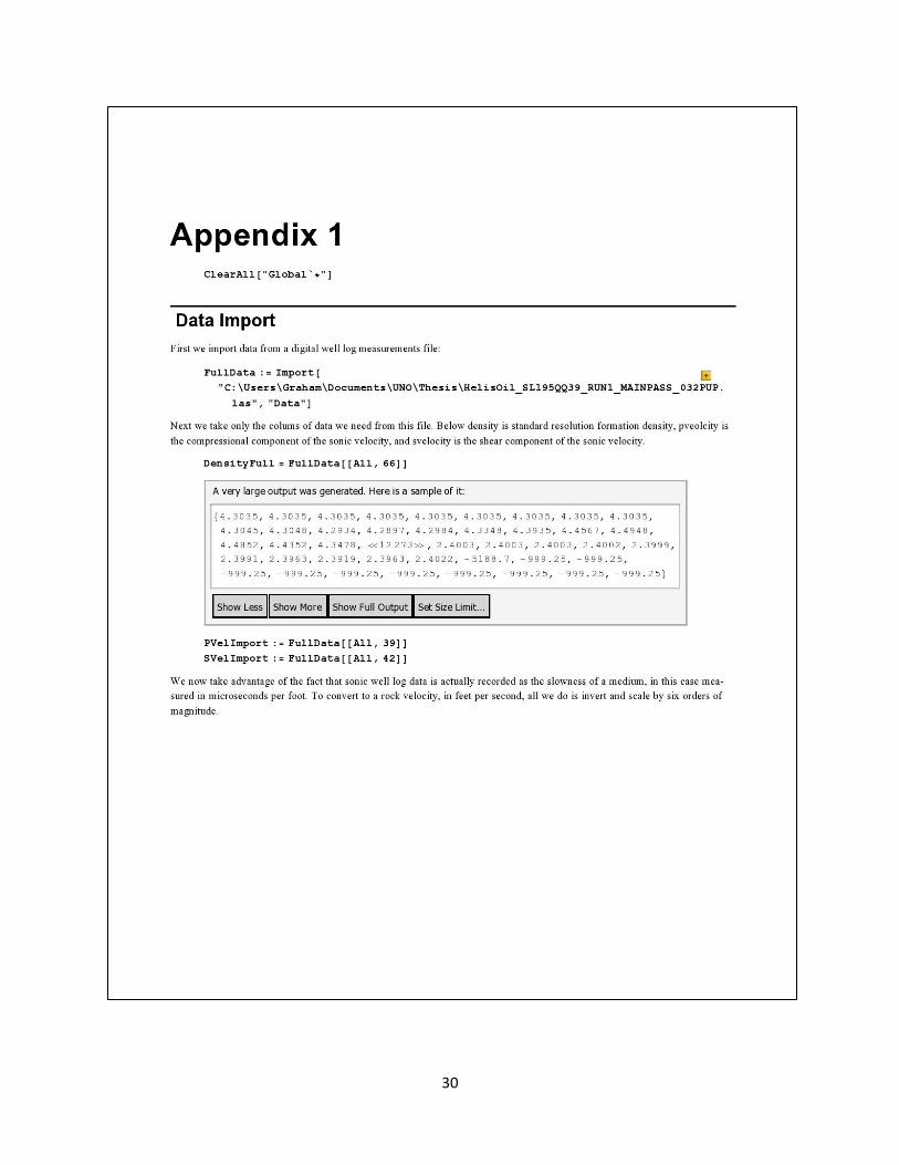
Data

The algorithm begins with the task of importing, categorizing, and sorting a large amount of data. Well

file data, in .las form, always comes as one large file per well with a large header including well

information such as location, owners, elevations, etc. The rest of the file contains data organized by

down-hole depth and separated into the various measurements taken during acquisition. The first step

is to separate the header from the file and keep the data in raw form. The data are imported and

organized into useable columns. Only three measurements are retained: bulk density ρ, compressional

delta time α, and shear delta time β.

Wavelet Choice

A good synthetic gather can determine the difference between drilling a productive well and a dry hole.

There are two simple ways of choosing a wavelet to use in practice. A very accurate method is to take a

subset of seismic data for analysis and frequency matching; this method will not be used in our

algorithm because comparison with seismic data is outside of the scope of this paper. The method we

employ is the computation of a theoretical wavelet with specified properties. We use a Ricker wavelet

with a form given by Ryan (1994) as

Eq. 5

where is the peak frequency and is time. This wavelet has Fourier transform

Eq. 6

where

An example Ricker wavelet with f =1 and its transform with peak at ω = 2 π f = 2 π = 6.28 are shown in

Figure 7. This wavelet is a natural choice as the single parameter defining it is the peak frequency of its

distribution.

11

Another mandatory constraint on synthetic wavelets is the zero phase requirement; a zero phase

wavelet has its impulse response centered on the reflection coefficient data. The Ricker is also a zero

phase wavelet as seen in Figure 7 where the wavelet is symmetric with respect to the vertical axis. By

using more complicated combinations of sinc function wavelets one can more accurately approximate a

real seismic signal; however, for our purposes the Ricker wavelet works well.

Figure 7: (left) Ricker wavelet r(t) with f = 1, (right) its Fourier transform R(ω)

Normal Incidence Synthetic Trace

Acoustic impedance is the density of the medium multiplied by the velocity of sound in the medium. For

a normally incident wave at a plane boundary in an isotropic medium, the reflection coefficient is the

ratio of the amplitude of the reflected wave to the amplitude of the incident wave. After some algebra

we obtain

Eq. 7

where is the density of the medium and α is the velocity of a p wave in the same medium (see Figure

4). By convolving the equation 7 with equation 5 we can construct a synthetic seismogram:

Eq. 8

where n is data index number and t is time. With sampled data, the integral becomes a sum in the linear

discrete convolution:

Eq. 9

where N is the index of the deepest depth in the oil well and the number of data samples is N. Figure 8

shows a convolution produced by using equation 9 with r(t) the Ricker wavelet and RC the reflection

coefficients from well log data. The trace in Figure 8 has been edited in the following ways to match

1.0 0.5 0.5 1.0

0.4

0.2

0.2

0.4

0.6

0.8

1.0

5 10 15 20 25 30

0.05

0.10

0.15

amplitude amplitude

time (s)

frequency (radian)

12

industry standards: the positive peaks of the waveform have been filled in to the axis, and the plot has

been rotated to simulate a vertical section of data, with index number increasing down.

Figure 8: The normal trace plotted by using the ratio of reflected amplitude to incident amplitude for the reflection

coefficient series of Eq. 7, from well log data, convolved with the Ricker wavelet of Eq. 5.

The positive peaks of the waveform are hard kicks (to the right) created by an interface between a low

acoustic impedance and a deeper high acoustic impedance, and the negative peaks, or troughs, of the

waveform are soft kicks (to the left) created by an interface between a high acoustic impedance and a

deeper low acoustic impedance. The horizontal scale is a dimensionless qualitative measure of reflection

strength, here normalized to 0.2.

2040

6080

100120

0.2

0.1

0.0

0.1

0.2

Amplitude

Data Index

13

Note that this is only a simulation of depth indexed data because the reflection coefficient data are

indexed by increasing data number only. If the data were to be used in the field to create time-depth

pairs on a seismic section we would need to re-index the data using the local velocity function.

Offset Incorporation and AVO

While the properties of this one trace are interesting in the sense that they give us a qualitative mapping

of rock properties to time migrated seismic data, we need to take another step and consider the effects

of an offset angle. In chapter 1 we showed the Zoeppritz equations (Eq. 1). This set of coupled equations

is too complex to be useful in a computational manner because it contains solutions to converted phase

waves which we don’t need, so we use the Aki-Richards linear approximation to these equations (Aki

and Richards, 2002).

Eq. 10

where

and are the p wave velocities of layers 1 and 2, are the s wave velocities, are the

densities, are the angles from the Zoeppritz equations, and P is the ray parameter given

after equation 2. Again, Figure 4 shows these angles in a graphical form.

Equation 10 is dependent on mixed angles and wireline log measurement coefficients. In our

formulation we use equation 10 in a slightly different form: that of Hilterman and Graul (2009) which,

following Aki and Richards, assumes similar properties between adjacent media:

14

Eq. 11

This equation is dependent on the wireline log properties and the angle of incidence for a down-going

primary wave. We set the offset angle to zero for normal incidence in the Aki-Richards equation and use

our algorithm to plot one trace, seen in Figure 9.

Figure 9: A zero offset trace plotted using the Aki-Richards equation

2040

6080

100120

0.2

0.1

0.0

0.1

0.2

Amplitude (dB)

Data Number (unitless)

15

This plot is identical to the normal trace plot of Figure 8 obtained using the normal angle reflection

coefficient equation. This can be verified by entering a zero degree incidence angle in the Aki-Richards

equation (Eq. 11) to produce the incident angle reflection coefficient equation (Eq. 7).

To obtain the reflection coefficients for other offset angles we can insert the desired angle and the

wireline log data into the Aki-Richards equation (Eq. 11). For the plots and results below (following

industry standards) we use angles from zero to fifty degrees in increments of five degrees. It is possible

to use any angle desired up to the critical reflection angle of total internal reflection, where the

equations no longer hold (Telford, 1990).

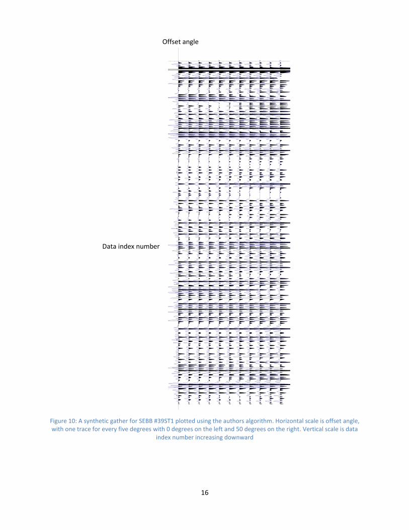
In Figure 10 a convolution is used to combine the reflection coefficient data with the wavelet as was

done for Figure 9. As is industry standard, the angle increases left to right. The trace of Figure 9 is the

left-most trace of Figure 10, at zero offset angle. Other parameters are the same as above. There is an

extra multiplicative factor in front of the convolution to normalize the results so they scale correctly on

the same plot.

Figure 10 is an industry standard synthetic gather created using the author’s algorithm. The horizontal

axis is offset angle, with one trace for every five degrees of offset angle (θ1 from Figure 4). The vertical

scale is data index number, increasing downward. As is standard for all seismic data, synthetic and

measured, the positive peaks (or peaks) of each waveform are filled in to the zero crossing, and the

negative peaks (or troughs) are left unfilled.

16

Figure 10: A synthetic gather for SEBB #39ST1 plotted using the authors algorithm. Horizontal scale is offset angle, with one trace for every five degrees with 0 degrees on the left and 50 degrees on the right. Vertical scale is data

index number increasing downward

2040

6080

100120

10 20 30 40 50

Data index number

Offset angle

17

Chapter 4: Analysis

As was shown in chapter 3, the method we use to create a synthetic seismic gather is based on response

to changing media and increasing offset angle. It can provide a basis for geophysical analysis to be done

in the field later if seismic data has been acquired over the area. The question remains: is it more or less

accurate than the other approximations used in the field today?

Due to the high cost of commercial software packages, the author only has access to one: IHS Kingdom.

Using Kingdom we create a synthetic gather for the same oil well described in chapter 3; this Kingdom

synthetic gather is shown in Figure 11.

Figure 11: A synthetic gather of SEBB #39ST1 plotted using IHS Kingdom

Figure 11 is an industry standard commercial synthetic gather. The horizontal axis is offset angle, with

one trace for each degree with 0 degrees on the left and 50 degrees on the left. The vertical scale is

measured depth in feet of the well from the top of the wireline log data to the bottom of this data. The

Depth (ft)

Offset angle

18

horizontal orange dashed lines are depth indicators called formation tops that help the geophysicist to

define the gather while manipulating it. As is standard for all seismic data, synthetic and measured, the

positive peaks (or peaks) of each waveform are filled in to the zero crossing, and the negative peaks (or

troughs) are left unfilled.

Algorithm Differences

As we can see the above Kingdom synthetic gather (Figure 11) is somewhat different from ours (Figure

10). There are several reasons for this: first, the vertical scales are different. Second, the wavelets are

slightly different. Third, the sample rates are different. And finally, as is the aim of this paper to

investigate, the linear approximation to the Zoeppritz equations is different. All of these differences are

discussed in detail below.

1) Vertical Scale

The scale on the vertical axis on the Kingdom gather (Figure 11) is obviously more gross then the scale

on our gather (Figure 10). The stretch and squeeze on the overall picture makes it difficult for the eye to

pick out where the peaks and troughs of the waveform match between gathers. The indexing in the

Kingdom gather is in subsea feet, where as the indexing in our gather is as increasing data samples

which distorts the image somewhat. The image scaled to our specifications is more accurate than the

commercial software. Our gather has been rescaled for a more detailed comparison discussed below

and shown in Figure 17.

Figure 12 shows the data index to depth map we use in our algorithm, representative of a time-depth

chart in a commercial setting. Time-depth charts are used to create velocity profiles from the synthetic

gather to scale borehole distances to match seismic data. Figure 12 with its constant linear slope

indicates a constant velocity. Figure 13 is the velocity function created by using a simple finite

differencing algorithm to calculate the discrete derivative of the data index/depth map shown in Figure

12. Figure 13 shows the constant velocity as predicted by Figure 12.

19

Figure 12: A data index/depth map from the author's algorithm

Figure 13: The discrete derivative of the data in figure 12

20 40 60 80 100 120index

3000

4000

5000

6000

7000

8000

depth ft

3000 4000 5000 6000 7000 8000depth ft

0.5

1.0

1.5

2.0

differential

20

Figure 14 is a time-depth map created by using the data from the synthetic gather in IHS Kingdom. This

plot is slightly non-linear which indicates variations in the velocity function. Figure 15 is the velocity

function created from Figure 14 using the same finite differencing algorithm as is used to produce Figure

13 from Figure 12. Figure 15 shows the non-linearity in the velocity function used by the commercial

software, the source of the stretch/squeeze inconsistencies shown in the vertical scale in Figure 17.

Note that the vertical scales of Figure 13 and Figure 15 are very different.

Figure 14: A time/depth map from IHS Kingdom

0.2 0.4 0.6 0.8 1.0time s

2000

4000

6000

8000

depth ft

21

Figure 15: The discrete derivative of the data in figure 14

2) Wavelets

The wavelet in the Kingdom gather is a frequency-matched wavelet. A frequency-matched wavelet is

defined as derivatives of cardinal B-splines. It visually resembles an Ormsby wavelet, defined by Ryan

(1994) as

Eq. 12

where f1 is the low no-pass frequency, f2 is the low full-pass frequency, f3 is the high full-pass frequency,

f4 is the high no-pass frequency, and (Bracewell, 2000)

The Ormsby wavelet has Fourier transform

Eq. 13

2000 4000 6000 8000Depth ft

0.05

0.10

0.15

Differential s

22

where we use Bracewell’s triangle function

For visual comparison with our wavelet (Figure 7) we have plotted an Ormsby wavelet and its Fourier

transform in Figure 16.

Figure 16: (left) an Ormsby wavelet and (right) its Fourier transform

The Kingdom wavelet is a close approximation to the Ormsby wavelet. The Ormsby-Kingdom wavelet

and the Ricker wavelet have noticeably different shapes and passbands. The Ormsby is quite different

from the Ricker wavelet as seen when comparing Figure 7 to Figure 16. Therefore, the Kingdom wavelet

is also quite different from the Ricker wavelet. These variations account for differences in the shape of

the traces of the author’s gather when compared to the Kingdom gather. With our simply defined Ricker

we can only vary the peak frequency, which when decreased broadens the wavelet and therefore low

pass filters more in the convolution. When the frequency is increased the wavelet becomes more

compressed which smoothes less (sharpens) in the convolution.

3) Sample Rates

A major difference between the two synthetic gathers is that the sample rates are different. The

Kingdom gather uses many fewer samples than we do in our algorithm. The result is heavy aliasing of

the high frequency response in the gather. Of course, this sparse sampling decreases processing time

dramatically and is also one of the reasons why the Kingdom gather looks smoother than our gather. In

Figure 17 we will show that the result of using a smoothing filter and sample rate reduction on our

gather more closely matches the results from Kingdom.

4) Approximations

The Kingdom gather (Figure 11) uses a three term Shuey approximation to the Zoeppritz equations. In

Shuey’s (1985) original notation,

1.0 0.5 0.5 1.0

5

5

10

1 2 3 4 5

0.2

0.4

0.6

0.8

1.0

Amplitude Magnitude

Frequency (Hz)

Time (s)

23

Eq. 14

whereas our gather uses the Aki-Richards approximation to the Zoeppritz equations (stated in Eq. 10).

Comparison of the two synthetic gathers

Figure 17: Synthetic gathers, (left) created using IHS Kingdom, (right) created using the author's algorithm

24

Figure 17 is a scaled, correlated comparison of the synthetic gather created using IHS Kingdom (left) and

using our new algorithm (right). The two gathers are depth matched, phase rotated, and wavelet

frequency scaled to match each other as well as possible for comparison of the AVO response. Recall

that the Zoeppritz approximations are different for the two gathers. On the side of each image are

colored dots. Each colored dot indicates the same event on the two gathers. The horizontal dashed

orange lines in the Kingdom gather are formation top indicators, used in the software to compare

seismic data to synthetic gathers. The major reflectors of Figure 17 in each case respond in the same

way to an increase in offset.

Depth matching is begun by using a linear shift of the author’s synthetic gather’s datum (starting depth)

to match that of the Kingdom synthetic gather. This is necessary because the data in the commercial

synthetic gather are extrapolated on both ends as seen in the time-depth map in Figure 14, where

depths of less than two thousand feet and greater than eight thousand feet are included. Depth

matching is accomplished by adding a translation term, , to the convolution of equation 9:

Eq. 15

Phase rotation is a linear phase modulation of each synthetic trace of the author’s algorithm to match

the peaks and troughs of the waveform to that of the commercial Kingdom gather. This is necessary

because for visual comparison of two synthetic gathers you must be able to correlate one waveform

event (peak, trough, or zero crossing) to the same event on both gathers. Though there are several ways

to do this, the simplest is to add a translation term, , to the Ricker wavelet before convolution;

obviously will be smaller than the period of the wavelet. Therefore equation 5 is modified to be

Eq. 16

Wavelet frequency scaling for the Ricker wavelet dilates or contracts the wavelet to smooth or sharpen

the trace, respectively. For the Ricker wavelet this is done by changing the peak frequency, f, in equation

16. A smaller f will dilate the wavelet causing more-low pass filtering in the convolution, which creates a

smoother waveform. A larger f will contract the wavelet allowing more high frequency through the filter

in the convolution, which creates a sharper trace.

Next, consider the AVO response of reflectors. Figure 18 and 19 are representations of class 1 and class

4 AVO responses, respectively. In the left panel PR stands for Poisson’s ratio, and AI stands for acoustic

impedance. The right panel shows the decrease or increase in amplitude with respect to increasing

offset angle. Class 1 (Figure 18) AVO seismic events decrease in magnitude (positive or negative

amplitude) with increasing offset angle. Class 4 AVO (Figure 19) seismic events increase in magnitude

(positive or negative amplitude) with increasing offset angle.

25

Figure 18: A cartoon of a class 1 AVO response (Hampson-Russell, 2005)

Figure 19: A cartoon of a class 4 AVO response (Hampson-Russell, 2005)

In both panels of Figure 17 we can see a wavelet doublet split with increasing offset angle at the green

marker around 3400 feet. This shows a class 1 AVO response (Hampson-Russell 2005) in which a large

positive reflector decreases to a small positive reflector with increasing offset. Another example is at the

yellow marker around 6200 feet where we see a decrease in amplitude with respect to increasing offset

angle. These class 1 AVO responses can be correlated to the type of lithology causing each reflection

event, and whether or not these zones are hydrocarbon bearing.

Futhermore, in Figure 17 between the blue marker at 5800 feet and the yellow marker at 6200 feet in

the commercial synthetic gather we see very little in terms of AVO changes. However, in the author’s

synthetic gather there is a well defined doublet exhibiting class 4 AVO behavior, in which a small positive

event increases to a large positive event (Hampson-Russell 2005) shown in Figure 19.

Phase reversal describes the tendency of a seismic event to change from a peak to a trough or vice

versa. The Kingdom gather uses a three term Shuey approximation to the Zoeppritz equation (Eq. 13),

which is not as sensitive to phase reversal in offset response as the Aki-Richards approximation

26

(Marfurt, 2008). This lack of sensitivity is detrimental in hydrocarbon exploration as the phase reversal

of a booming reflector can change the interpretation by the geophysicist.

In Figure 10 it is shown that our algorithm can create a very detailed synthetic seismic gather. To create

such a detailed image requires increased processing time because of the large number of calculations in

the convolution of equation 9 when spread across twenty five traces. The Kingdom synthetic gather of

Figure 11 is less detailed, but is computed more than an order of magnitude faster than our algorithm.

However, our algorithm has not been optimized for speed, so some decrease in processing time can be

anticipated.

27

Chapter 5: Conclusions and Future Work

Conclusions

Our algorithm can detect fine differences in the AVO response of seismic events. This is due to the

nature of the Aki-Richards approximation (Eq. 10) to the Zoeppritz equations (Eq. 1) being organized into

terms describing rock properties, rather than by terms describing increasing offset angles as in the

Shuey approximation (Eq. 14), indicative of the types of better definition we expect to see overall from

the Aki-Richards approximation.

When our synthetic gather is scaled to the standard size/resolution of the commercial Kingdom

synthetic gather, as in Figure 17, image quality is lost. This blurring should be noted when using any

commercial software to create synthetic gathers.

The author’s algorithm is computationally slow enough that it would be a computing time burden if used

in a commercial setting. Our algorithm could easily be optimized for speed, however.

Future Work

To extend the author’s synthetic gather to a volume of seismic data, a non-linear velocity function would

be necessary. This velocity function, as mentioned in chapter 4, is needed to change the scaling of the

synthetic gather to relate the lithologic units in the well bore to the events in the seismic data. The

scaling would necessarily change the resolution of some of the seismic events seen in the synthetic

gather, as the reflection coefficients would be distributed differently in vertical depth.

Once properly velocity-corrected it would be possible to start data interpretation on the seismic volume.

With the same data set, one interpreting geophysicist could create two different interpretations using

our synthetic gather and the Kingdom synthetic gather. The data sets could be time shifted and the

interpreted formation tops could be subtracted for a quantitative comparison of the two synthetic

gathers in depth.

There are several other research topics for the future. First, one could use a wavelet convolution (Strang

and Nguyen, 1990) to combine the reflection coefficients with the wavelet. Second, using a fast super-

computer, every sample (without averaging) could be used to compare the seismic response to the

current (sample averaged) version of the gather. Finally, third and most useful, the same algorithm

could be used with different approximations to the Zoeppritz equations to create different synthetic

gathers and difference gather panels calculated to compare AVO anomaly behavior.

28

References

Aki, Keiiti. Richards, Paul G. 2002. Quantitative Seismology, 2nd ed. University Science Books.

Asquith, George. Krygowski, Daniel. 2004. AAPG Methods in Exploration Series, No. 16. “Basic Well Log Analysis, 2nd ed” Tulsa, OK: American Association of Petroleum Geologists.

Bacon, M. et al. 2007. 3-D Seismic Interpretation. New York, NY: Cambridge University Press.

Bracewell, Ronald N. 2000. The Fourier Transform and It’s Applications. Singapore: McGraw-Hill.

Glover, Paul. “The Sonic or Acoustic Log”. Universite Laval. <http://www2.ggl.ulaval.ca/personnel/paglover/CD%20Contents/GGL-66565%20Petrophysics%20English/Chapter%2016.PDF>

Hampson-Russel inc. 2005. “AVO Classes Reference Guide”. <http://www.cggveritas.com/data/1/rec_docs/591_avo_classes_reference_guide.pdf>

Hilterman, Fred. Graul, Mike. 2009. SEG Continuing Education Course. “Seismic Lithology”. Continuing Education Series.

Marfurt, Kurt J. Chopra, Sattinder. 2008. Seismic Attributes for Prospect Identification and Reservoir Characterization. Tulsa, OK: Society of Exploration Geophysicists.

Meunier, Julien. 2011. 2011 Distinguished Instructor Short Course. “Seismic Acquisition from Yesterday to Tomorrow”. Distinguished Instructor Series, No. 14: Society of Exploration Geophysicists.

Ryan, Harold. 1994. “Ricker, Ormsby, Klauder, Butterworth – A Choice of Wavelets”. Hi-Res Geoconsulting. Canadian Society of Exploration Geophysicists. <http://www.cseg.ca/publications/recorder/1994/09sep/sep94-choice-of-wavelets.pdf>

Sheriff, Robert E. 1991. Encyclopedic Dictionary of Exploration Geophysics. Tulsa, OK: Society of Exploration Geophysicists.

Shuey, R. T. 1985. "A simplification of the Zoeppritz equations". Geophysics 50 (9): 609–614.

Strang, Gilbert. Nguyen, Truong. 1997. Wavelets and Filter Banks. Wellesley MA: Wellesley-Cambridge Press.

Telford, W.M., et al. 1990. Applied Geophysics, 2nd ed. New York, NY: Cambridge University Press.

Upadhyay, S.K. 2004. Seismic Reflection Processing with Special Reference to Anisotropy. Berlin, Germany: Springer-Verlag.

VerWest, Bruce. 2004. “Elastic Impedance Revisited”. Houston, TX: Veritas DGC.

Zoeppritz, Karl. 1919. Erdbebenwellen VII. VIIb. Über Reflexion und Durchgang seismischer Wellen durch Unstetigkeitsflächen. Nachrichten von der Königlichen Gesellschaft der Wissenschaften zu Göttingen, Mathematisch-physikalische Klasse, 66-84.

29

Appendix The following is the algorithm the author wrote in the computational mathematics software, Mathematica, to create synthetic seismic gathers using the Aki-Richards approximation to the Zoeppritz equations.

30

31

32

33

34

35

36

37

38

39

40

41

42

43

44

45

46

47

48

49

50

51

52

53

54

55

56

57

Vita

The author was born in Baltimore, Maryland. He obtained his Bachelor’s degree in Physics from the

University of New Orleans in 2009. He joined the University of New Orleans graduate program to pursue

a Ph.D. in Engineering and Applied Science with a concentration in geophysics. He is an active processing

and interpretive geophysicist employed by his own company, Sandstone Oil and Gas, in New Orleans. He

is a member of the Southern Geophysical Society, Society of Exploration Geophysicists, American

Association of Petroleum Geologists, and the Geological Society of America.