Calculation of the stability index in parameter-dependent calculus of variations

problems: Buckling of a twisted elastic strut

Kathleen A. Hoffman1, Robert S. Manning2, and Randy C. Paffenroth3,

June 27, 2002

Abstract

We consider the problem of minimizing the energy of an inextensible elastic strut with length 1 subject toan imposed twist angle and force. In a standard calculus of variations approach, one first locates equilibria bysolving the Euler-Lagrange ODE with boundary conditions at arclength values 0 and 1. Then, one classifies eachequilibrium by counting conjugate points, with local minima corresponding to equilibria with no conjugate points.These conjugate points are arclength values σ ≤ 1 at which a second ODE (the Jacobi equation) has a solutionvanishing at 0 and σ.

Finding conjugate points normally involves the numerical solution of a set of initial value problems for theJacobi equation. For problems involving a parameter λ, such as the force or twist angle in the elastic strut, thiscomputation must be repeated for every value of λ of interest.

Here we present an alternative approach that takes advantage of the presence of a parameter λ. Rather thansearch for conjugate points σ ≤ 1 at a fixed value of λ, we search for a set of special parameter values λm(with corresponding Jacobi solution ζm) for which σ = 1 is a conjugate point. We show that under appropriateassumptions, the index of an equilibrium at any λ equals the number of these ζm for which 〈ζm,Sζm〉 < 0, whereS is the Jacobi differential operator at λ. This computation is particularly simple when λ appears linearly in S.

We apply this approach to the elastic strut, in which the the force appears linearly in S, and as a result, welocate the conjugate points for any twisted unbuckled rod configuration without resorting to numerical solutionof differential equations. In addition, we numerically compute 2-dimensional sheets of buckled equilibria (as thetwo parameters of force and twist are varied) via a coordinated family of one-dimensional parameter continuationcomputations. Conjugate points for these buckled equilibria are determined by numerical solution of the JacobiODE.

Keywords: elastic rods, anisotropy, stability index, conjugate points, buckling, parameter con-

tinuation, isoperimetric constraints

AMS Subject Classifications: 49K15, 34B08, 74K10, 74G60, 65P30, 65L10

1Department of Mathematics and Statistics; University of Maryland, Baltimore County; Baltimore, MD 21250 USA;khoffman@math.umbc.edu

2Mathematics Department; Haverford College; Haverford, PA 19041 USA; rmanning@haverford.edu3Applied and Computational Mathematics; California Institute of Technology; Pasadena, CA 91125 USA; redrod@acm.org

1

1 Introduction

The classification of equilibria is a familiar idea from finite-dimensional optimization. Given an

equilibrium (or critical point) of a function, one computes the eigenvalues of the Hessian matrix, and

determines the type of the equilibrium by computing the index, the number of negative eigenvalues.

Equilibria with index 0 are local minima, those with index 1 are saddle points with one downward

direction, etc. The goal is analogous in infinite dimensions, when the quantity J to be optimized

is itself a function of a function q(s), say with 0 ≤ s ≤ 1.4 Now the equilibria q0(s) are found by

solving the Euler-Lagrange ordinary differential equation (ODE). The role of the Hessian is played

by the second-variation operator, and the notion of index, the number of negative eigenvalues in

the spectrum of this operator, remains, with local minima again characterized as having index 0.

In many applications, s is a spatial variable and J a potential energy,5 and we think of the index as

determining “stability”, with the idea that when time-dependence and a kinetic energy are added

to this potential energy, the index-0 local minima will likely be dynamically stable. We emphasize,

however, that in this paper, “stability” is purely a classification of the type of an equilibrium for

an optimization problem.

In the calculus of variations, there is a powerful theory that allows a relatively simple determina-

tion of the index (see, e.g., [9]). Given an equilibrium, one consider the associated Jacobi equation,

a linear second-order ODE. One then defines the notion of a conjugate point, which is a number σ

such that the Jacobi equation has a nonzero solution that vanishes at s = 0 and s = σ. Jacobi’s

strengthened condition says that the equilibrium is a local minimum if it has no conjugate point in

(0, 1]. Morse [20] later generalized this theory to show that, assuming 1 is not a conjugate point,

the number of conjugate points in (0, 1) is the index of the equilibrium. This Euler-Jacobi-Morse

index theory thus achieves a remarkable simplification: it reduces the problem of counting the

number of negative eigenvalues of the second variation operator of J in infinite-dimensional space

to the problem of solving a second-order ODE and counting conjugate points. Thus, the only nu-

merical approximation arises in the discretization of ODEs, namely the Euler-Lagrange and Jacobi

equations.

Here we present a further simplification applicable to parameter-dependent problems, and es-

pecially problems in which a parameter λ appears linearly in the second variation, for example,

in problems containing a Lagrange multiplier. In this case, the counting of conjugate points at

σ ≤ 1 for a fixed value of λ can be reduced to the problem of analyzing conjugate points at the

fixed value σ = 1 as λ is allowed to vary. Often, the determination of conjugate points at σ = 1 is4To rigorously define optimization in infinite dimensions, a normed space must be specified for the input functions q. Following

standard practice, we use the C1([0, 1]) norm, in which case the resulting minima are traditionally referred to as “weak minima” [9].5We note in passing an interesting exception. When J is a Lagrangian action functional, and s represents time, the equilibria are

classical mechanical trajectories, and the index plays a crucial role in the semiclassical approximation of these trajectories as quantummechanical limits are approached [13]. The example in this paper involves a potential energy functional, but the general theory presentedcould equally well be applied to the determination of the semiclassical index for classical trajectories dependent on some parameter.

2

easier than the general analysis of conjugate points for σ ≤ 1, so this reduction can be a significant

simplification. Of course, in cases where the relevant differential equations can not be solved in

closed form, this simplification is impractical, and one must revert to computing conjugate points

numerically.

We further show that this entire theory can be carried through to the case of problems with

isoperimetric constraints, where the only required change is an update to the definition of conjugate

point. This updated definition of “constrained conjugate point” is the one taken, e.g., by Bolza [2],

and rephrased in functional analytic language in Manning, Rogers, and Maddocks [19].

We apply this method for direct index computation to the example of a thin elastic strut with

elliptical (anisotropic) or circular (isotropic) cross-section, under the constraints shown in Fig. 1.

One end of the rod is clamped at the origin, with the major axis of the ellipse along the x-axis,

Figure 1: An elastic strut clamped at each end, with a relative twist angle α, and with one end allowed to slidevertically in response to an imposed force λ. The cross-sections of the rod are elliptical, which we depict by showingthe curve through the centers of the cross-sections as a green tube, and tracking the major axes of the cross-sectionswith a blue ribbon.

the minor axis along the y-axis, and the tangent vector to the rod along the z-axis. The other

end is constrained to lie along the z-axis, with its tangent vector also along the z-axis, and its

cross-section twisted by an angle α with respect to the x-y plane, but can slide up and down the

z-axis in response to an applied vertical force λ.

Such a rod buckling problem has fed the curiosity of scientists since the time of Euler and La-

3

grange [17]. In 1883, Greenhill [11] considered the plane (over all values of α and λ) of unbuckled

configurations for an isotropic strut, and derived the condition for the index to be zero. More re-

cently, Champneys and Thompson [3] and van der Heijden et al [27] performed bifurcation analyses

of an anisotropic elastic rod, but did not focus on the question of stability. Goriely et al [10] con-

sidered the dynamic stability of the unbuckled configurations for both the isotropic and anisotropic

cases, and van der Heijden et al [26] inferred stability for unbuckled and buckled configurations for

the isotropic case from the shape of solution branches in a particular “distinguished” coordinate

system. Neukirch and Henderson [21] performed an in-depth classification of buckled solutions for

the isotropic problem, including the computation of two-dimensional sheets of equilibria.

Here we present stability results for this problem that both complement the results cited above

and serve as an illustration for the general index theory we develop. Specifically, this theory allows

a semi-analytic determination of the index on the plane of unbuckled configurations for both the

isotropic and anisotropic strut (semi-analytic in that it requires the numerical solution of an alge-

braic equation, but no differential equations). In addition, we compute sheets of buckled solutions

using a family of one-dimensional branches generated by the parameter continuation package AUTO

[5, 6]. We determine the index of configurations on these sheets via a numerical implementation of

the conjugate point test developed in [19], since a closed-form solution of the differential equations

is not feasible in this case.

We begin in Sec. 2 by reviewing conjugate point theory for unconstrained and constrained prob-

lems. Sec. 3 presents our direct method for computing the index for unconstrained problems, which

is then extended to problems with isoperimetric constraints in Sec. 4. In Sec. 5, we summarize the

standard Kirchhoff theory of inextensible and unshearable elastic struts. The index on the plane of

unbuckled equilibria for both the isotropic and anisotropic strut is determined in Sec. 6, and the

buckled configurations and their stability are presented in Sec. 7.

2 A Review of Conjugate Point Theory

2.1 Unconstrained Conjugate Points

In this section, we summarize conjugate point theory for unconstrained calculus of variations prob-

lems. This theory is an established part of the classic unconstrained calculus of variations literature

and can be found in many standard texts, e.g. [7, 9, 14, 24]. However, index theory appears only

in more modern treatments [12, 20].

We consider a functional of the form:

J [q] =

∫ 1

0

L(q,q′, s) ds, q(s) ∈ Rp,

subject to q(0) = h0, q(1) = h1.

(1)

Equilibria q0(s) are solutions to the standard Euler-Lagrange equations for the functional J . Clas-

4

sification of these equilibria involves an analysis of the second variation of J at q0, namely

δ2J [ζ] =1

2

∫ 1

0

[(ζ ′)TPζ ′ + (ζ ′)TCTζ + ζTCζ ′ + ζTQζ

]ds, (2)

for P ≡ L0q′q′ , C ≡ L0

qq′ , and Q ≡ L0qq, where here and throughout, superscripting by T denotes the

transpose, subscripting by q or q′ denotes partial differentiation, and superscripting by 0 denotes

evaluation at q0(s). We assume that Legendre’s strengthened condition holds

P > 0, (3)

i.e. the symmetric matrix P is positive definite. Here ζ is a variation in q that, due to the boundary

conditions on q, must lie in the set of admissible variations:

Hd ≡{ζ ∈ H2(Rp, (0, 1)) : ζ(0) = ζ(1) = 0

}.

Here we have chosen the Sobolev space H2 of functions with integrable weak second derivatives

because after an integration by parts, the second variation will take the form:

δ2J [ζ] =1

2〈ζ,Sζ〉,

where S is the self-adjoint second-order vector differential operator:

Sζ ≡ − d

ds

[Pζ ′ + CTζ

]+ Cζ ′ + Qζ, (4)

and 〈·, ·〉 denotes the usual inner product in L2(Rp, (0, 1)):

〈f ,g〉 =

∫ 1

0

[f(s)]Tg(s) ds.

A sufficient condition for q0 to be a local minimum of J is a combination of Legendre’s strength-

ened condition (3) with Jacobi’s strengthened condition that q0 has no conjugate point in (0, 1],

where a conjugate point is defined to be a value σ for which there is a nontrivial solution to:

Sζ = 0, 0 < s < σ, ζ(0) = ζ(σ) = 0. (5)

Morse [20] extended Jacobi’s condition to equate the number of conjugate points with the index

that quantifies the dimension of the set on which δ2J is negative.

In some cases, Eq. (5) can be solved analytically, but generically a numerical procedure for com-

puting conjugate points is required. For completeness, we briefly summarize a standard algorithm

for computing unconstrained conjugate points ([24], p. 152). We numerically compute a basis of

solutions {ζ1, . . . , ζp} to the homogeneous second-order initial value problem:

Sζ = 0, ζ(0) = 0. (6)

5

A conjugate point occurs when a nontrivial linear combination of {ζ1, . . . , ζp} vanishes, i.e., when

there is a nontrivial solution to the p× p linear system:

[ζ1 . . . ζp

] c1...cp

= 0. (7)

Therefore, as we build up solutions ζj(σ) to Eq. (6) as σ grows from 0 to 1, we track the determinant

of the p×p matrix[ζ1(σ) . . . ζp(σ)

], and count as a conjugate point every time this determinant

crosses zero.

2.2 Constrained Conjugate Points

In this section, we review a definition of conjugate point appropriate for calculus of variations

problems with isoperimetric constraints:

W [q] =

∫ 1

0

L(q,q′, s) ds, q(s) ∈ Rp,

subject to

∫ 1

0

gi(q) ds = 0, i = 1, . . . n,

q(0) = h0, q(1) = h1.

According to the usual multiplier rule, an associated functional

J [q] =

∫ 1

0

(L+ gTν

)ds

is constructed, and constrained equilibria (q0(s),ν0) of W are solutions of the standard uncon-

strained Euler-Lagrange equations for the functional J , with the multiplier ν0 determined by the

integral constraints. The second variation δ2J , and its associated operator S, take the unconstrained

forms (2) and (4), but now with Q = [g0qq]Tν0 + L0

qq. Admissible variations ζ must satisfy the

linearized constraints

〈ζ,Ti〉 = 0, i = 1, · · · , n,

where:

Ti ≡ (gi)0q.

We assume that the Ti(s) are linearly independent on (0, σ) for each σ ∈ (0, 1]. So, the admissible

set of constrained variations is:

Hconsd ≡ {ζ ∈ Hd : 〈ζ,Ti〉 = 0, i = 1, · · · , n} .

Bolza [2], citing work of Weierstrass and Kneser, defined the relevant notion of conjugate point

for an isoperimetric problem, namely that σ is called a conjugate point if the following system has

6

a nontrivial solution:

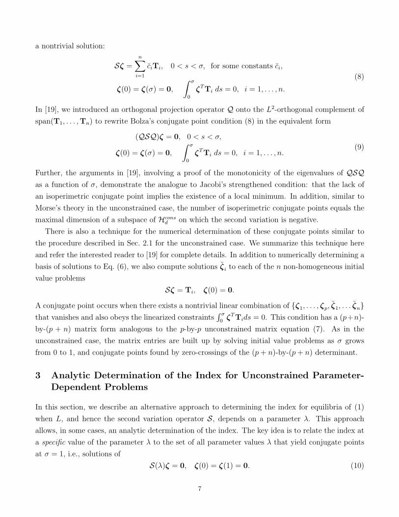
Sζ =n∑i=1

ciTi, 0 < s < σ, for some constants ci,

ζ(0) = ζ(σ) = 0,

∫ σ

0

ζTTi ds = 0, i = 1, . . . , n.

(8)

In [19], we introduced an orthogonal projection operator Q onto the L2-orthogonal complement of

span(T1, . . . ,Tn) to rewrite Bolza’s conjugate point condition (8) in the equivalent form

(QSQ)ζ = 0, 0 < s < σ,

ζ(0) = ζ(σ) = 0,

∫ σ

0

ζTTi ds = 0, i = 1, . . . , n.(9)

Further, the arguments in [19], involving a proof of the monotonicity of the eigenvalues of QSQas a function of σ, demonstrate the analogue to Jacobi’s strengthened condition: that the lack of

an isoperimetric conjugate point implies the existence of a local minimum. In addition, similar to

Morse’s theory in the unconstrained case, the number of isoperimetric conjugate points equals the

maximal dimension of a subspace of Hconsd on which the second variation is negative.

There is also a technique for the numerical determination of these conjugate points similar to

the procedure described in Sec. 2.1 for the unconstrained case. We summarize this technique here

and refer the interested reader to [19] for complete details. In addition to numerically determining a

basis of solutions to Eq. (6), we also compute solutions ζi to each of the n non-homogeneous initial

value problems

Sζ = Ti, ζ(0) = 0.

A conjugate point occurs when there exists a nontrivial linear combination of {ζ1, . . . , ζp, ζ1, . . . ζn}that vanishes and also obeys the linearized constraints

∫ σ0ζTTids = 0. This condition has a (p+n)-

by-(p + n) matrix form analogous to the p-by-p unconstrained matrix equation (7). As in the

unconstrained case, the matrix entries are built up by solving initial value problems as σ grows

from 0 to 1, and conjugate points found by zero-crossings of the (p+ n)-by-(p+ n) determinant.

3 Analytic Determination of the Index for Unconstrained Parameter-Dependent Problems

In this section, we describe an alternative approach to determining the index for equilibria of (1)

when L, and hence the second variation operator S, depends on a parameter λ. This approach

allows, in some cases, an analytic determination of the index. The key idea is to relate the index at

a specific value of the parameter λ to the set of all parameter values λ that yield conjugate points

at σ = 1, i.e., solutions of

S(λ)ζ = 0, ζ(0) = ζ(1) = 0. (10)

7

We will denote solutions to (10) by (λm, ζm), and refer to λm as branch points. This name is

appropriate since, in all cases we consider, new branches of equilibria will arise at λm. In many

applications, the analytic determination of (λm, ζm) is possible even when the general conjugate

point equation (5) can not be solved in closed form.

We will assume that {ζm} form a basis for Hd and that they are S-orthogonal, i.e., that

〈ζm,Sζn〉 = 0 for all m 6= n. These assumptions hold for many physically motivated problems,

including cases in which (10) is a standard Sturm-Liouville eigenvalue problem (see, e.g., [23, p.

273]). This basis of solutions can then be used to diagonalize S and determine the index directly,

as shown by the following lemma.

Lemma 1. Assume that {ζm} form an S-orthogonal basis of Hd. Then the index equals the number

of ζm for which 〈ζm,Sζm〉 < 0.

Proof. Let N be the subspace of Hd spanned by those ζm for which 〈ζm,Sζm〉 < 0. Any χ ∈ Hd

that is L2-orthogonal to N can be written as:

χ =∑ζm /∈N

cmζm

where the notation∑ζm /∈N denotes a sum over all m for which ζm /∈ N . Then by S-orthogonality,

〈χ,Sχ〉 =∑ζm /∈N

(cm)2〈ζm,Sζm〉.

By definition, 〈ζm,Sζm〉 ≥ 0 for all terms in the sum, so 〈χ,Sχ〉 ≥ 0.

Thus, N is a maximal subspace in Hd on which the second variation is negative. The index is

defined to be the dimension of N , which, by definition of N , is the number of basis functions ζm

for which 〈ζm,Sζm〉 < 0.

The above diagonalization is particularly useful when the parameter λ appears linearly in S:

Sζ = S1ζ + λS2ζ, (11)

because it is then routine to determine those basis functions ζm for which 〈ζm,Sζm〉 < 0. In fact,

the quantity 〈ζm,Sζm〉 is simply related to the λ-independent quantity 〈ζm,S2ζm〉 by the following

lemma.

Lemma 2. Suppose S takes the form (11). Then for any solution (λm, ζm) of (10),

〈ζm,Sζm〉 = (λ− λm)〈ζm,S2ζm〉.

8

Proof. The key idea is to exploit the fact that (S1 + λmS2)ζm = 0:

〈ζm,Sζm〉 = 〈ζm, (S1 + λS2)ζm〉

= 〈ζm, (S1 + λmS2 − λmS2 + λS2)ζm〉 = (λ− λm)〈ζm,S2ζm〉.

Lemmas 1 and 2 lead immediately to the following corollary, the central result of this article:

Corollary 1. If the solutions of (10) form an S-orthogonal basis for Hd, and if S has the form

(11), then the index of an equilibrium at parameter value λ equals the number of branch points λm

such that λ > λm and 〈ζm,S2ζm〉 < 0, plus the number of branch points λm such that λ < λm and

〈ζm,S2ζm〉 > 0.

Example (Planar buckling of a strut): We parametrize the strut by arclength s and choose a

length scale so that 0 ≤ s ≤ 1. We let θ(s) denote the angle that the strut makes with vertical at

position s. We impose the boundary conditions that the strut be vertical at s = 0 and s = 1, and

impose a vertical force λ. We then have the calculus of variations problem to minimize the total

energy ∫ 1

0

[1

2K(θ′(s))2 + λ cos(θ(s))

]ds, θ(0) = θ(1) = 0,

where K > 0 is a stiffness parameter.

Consider the unbuckled equilibrium θ(s) = 0. The second variation operator is Sζ = −Kζ ′′−λζ,

which is of the form (11), with S2 = −1. The nontrivial solutions to (10) are ζm(s) = A sin(mπs),

m = 1, 2, 3, . . . , with λm = m2π2. These solutions are an S-orthogonal basis for Hd, since S is a

Sturm-Liouville operator. We observe that 〈ζm,S2ζm〉 < 0 for all m, and then use Lemma 2 to

conclude that the sign of 〈ζm,S(λ)ζm〉 is the same as the sign of m2π2 − λ. Hence, we conclude

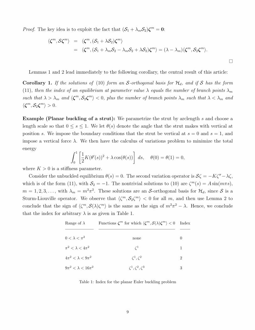
that the index for arbitrary λ is as given in Table 1.

Range of λ Functions ζm for which 〈ζm,S(λ)ζm〉 < 0 Index

0 < λ < π2 none 0

π2 < λ < 4π2 ζ1 1

4π2 < λ < 9π2 ζ1, ζ2 2

9π2 < λ < 16π2 ζ1, ζ2, ζ3 3

Table 1: Index for the planar Euler buckling problem

9

4 Analytic Determination of the Index for Isoperimetrically ConstrainedParameter-Dependent Problems

Next, we combine the ideas of the previous two sections to produce a method for directly comput-

ing the index in a calculus of variations problem with isoperimetric constraints, when the second

variation operator S depends on a parameter λ. As in Sec. 3, we assume that solutions ζm of

S(λ)ζ =n∑i=1

ciTi, 0 < s < 1, for some constants ci,

ζ(0) = ζ(1) = 0,

∫ 1

0

ζTTi ds = 0, i = 1, . . . , n

(12)

form an S-orthogonal basis for the relevant function space Hconsd . Although (12) reflects Bolza’s

definition of conjugate point at σ = 1, we will exploit the equivalence of (8) and (9) to rewrite

the differential equation S(λ)ζ =∑n

i=1 ciTi as (QS(λ)Q)ζ = 0. As before, the basis {ζm} will

be used to diagonalize the projected operator QSQ on Hconsd . In fact, Lemma 1 holds for the

constrained case, provided Hd is replaced with the space Hconsd , noting that since Q is self-adjoint,

〈ζ, (QSQ)ζ〉 = 〈ζ,Sζ〉 for ζ ∈ Hconsd .

If, in addition, S takes the form (11), then Lemma 2 can be extended to problems with isoperi-

metric constraints:

Lemma 3. Suppose S takes the form (11). Then for any solution ζm of (12),

〈ζm, (QSQ)ζm〉 = (λ− λm)〈ζm,S2ζm〉.

Proof. As in Lemma 2, the key idea is to exploit the fact that (Q(S1 + λmS2)Q)ζm = 0, combined

with the fact that Qζm = ζm for ζm ∈ Hconsd :

〈ζm, (QSQ)ζm〉 = 〈ζm, (Q(S1 + λS2)Q)ζm〉

= 〈ζm, (Q(S1 + λmS2 − λmS2 + λS2)Q)ζm〉

= 〈Qζm, (−λmS2 + λS2)Qζm〉

= (λ− λm)〈ζm,S2ζm〉.

Thus, the strategy for analytically determining the index in problems with isoperimetric con-

straints is the same as for unconstrained problems. This strategy will be illustrated in Sec. 6 for

the example of the buckling of an elastic strut under imposed force and twist. In preparation for

this example, we next summarize the basic elastic strut equations.

10

5 The Elastic Strut

5.1 Equilibrium equations

In the Kirchhoff theory of inextensible and unshearable elastic struts [1, 4, 16, 17], the configuration

of a strut is described by a centerline r(s) (written as a function of arclength s) and a set of directors

{d1(s),d2(s),d3(s)} that form an orthonormal frame giving the orientation of the cross-section of

the strut. For convenience, we choose a length scale so that 0 ≤ s ≤ 1. Let the superscript ′ denote

a derivative with respect to s. The assumptions of inextensibility and unshearability of the strut

are incorporated in the requirement that d3(s), the director orthogonal to the strut cross-section,

equals r′(s), the tangent vector to the centerline.

Orthonormality of the directors implies the existence of a (Darboux) vector u(s) defined by the

kinematic relations:

d′i(s) = u(s)× di(s), i = 1, 2, 3.

The components of u in the strut frame are denoted by ui(s) = u(s) · di(s) and are called the

strains.

It will be convenient to describe the directors via Euler parameters or quaternions q ∈ R4.

Quaternions provide an alternate formulation to Euler angles for parametrizing rotation matrices

in SO(3), see, e.g., ([25], p. 462). The directors di are the columns of a rotation matrix and can

be expressed by rational functions of the quaternions:

d1 =1

|q|2

q21 − q2

2 − q23 + q2

4

2q1q2 + 2q3q4

2q1q3 − 2q2q4

, d2 =1

|q|2

2q1q2 − 2q3q4

−q21 + q2

2 − q23 + q2

4

2q2q3 + 2q1q4

,d3 =

1

|q|2

2q1q3 + 2q2q4

2q2q3 − 2q1q4

−q21 − q2

2 + q23 + q2

4

,and therefore the strains can be expressed as:

u1 =2

|q|2(q′1q4 + q′2q3 − q′3q2 − q′4q1) , u2 =

2

|q|2(−q′1q3 + q′2q4 + q′3q1 − q′4q2) ,

u3 =2

|q|2(q′1q2 − q′2q1 + q′3q4 − q′4q3) .

For convenience, we define d3i(s) to be the ith component of the vector d3. We impose the

following constraints on the elastic strut:∫ 1

0

d31(q(s)) ds =

∫ 1

0

d32(q(s))ds = 0, q(0) = (0, 0, 0, 1), q(1) = (0, 0, sin(α/2), cos(α/2)). (13)

The boundary condition on q(0) forces the s = 0 end of the strut to be tangent to the z-axis. The

pair of integral constraints imply, due to the inextensibility-unshearability condition r′(s) = d3(s),

that x(0) = x(1) and y(0) = y(1), i.e., that the s = 1 end of the strut lies directly above the s = 0

11

end. Finally, the boundary condition on q(1) implies that the s = 1 end of the strut is tangent to

the z-axis and twisted by an angle α with respect to the s = 0 end. Fig. 1 depicts a solution that

satisfies Eq. (13).

The elastic energy of the strut is expressed in terms of the strains, and we assume here a

commonly used quadratic energy:

E[q] ≡∫ 1

0

[3∑i=1

1

2Ki [ui(q(s),q′(s))]

2+ λd33

]ds,

where Ki are the bending (i = 1, 2) and twisting (i = 3) stiffnesses of the strut, and λ is a force

pushing downward on the strut. Unbuckled twisted equilibria are described by:

q0(s) =

00

sin(αs2

)cos(αs

2)

,which correspond to directors

d1 =

cos(αs)sin(αs)

0

, d2 =

− sin(αs)cos(αs)

0

, d3 =

001

.These are readily verified to be solutions to the Euler-Lagrange equations of the functional E. The

goal of Sec. 6 is to use the theory of Sec. 4 to assign to these configurations a stability index.

5.2 The second variation

In this section, we show a routine but technical computation of the second variation of E, finding in

the end that it takes the form S = S1 +λS2 required for our results. The computation is somewhat

involved due to our choice to parametrize SO(3) by four-dimensional quaternions.

As outlined in Sec. 2.2, for each equilibrium q0, we define an allowed variation to be any δq so

that δq(0) = δq(1) = 0 and 〈δq, (d3i)0q〉 = 0 for i = 1, 2. The second variation of E is

δ2E[δq] =

∫ 1

0

[(δq′)TL0

q′q′δq′ + (δq′)TL0

q′qδq + (δq)TL0qq′δq

′ + (δq)TL0qqδq

]ds, (14)

where L is the integrand of E with the appropriate Lagrange multiplier terms added to it.

We note first a property of δ2E peculiar to the example at hand. The integrand L is invariant

to a scaling of q, i.e.,

L(cq, cq′) = L(q,q′)

for any c ∈ R. This degeneracy arises from our use of four-dimensional quaternions to represent the

three-dimensional space SO(3) of directors. If we write δq(s) as β(s)q0(s) + w(s) where at each s,

w(s) is perpendicular to q0(s), then

E[q0 + εδq] = E[(1 + εβ)q0 + εw] = E[q0 +ε

1 + εβw].

12

Therefore, E[q0 + εδq] < E[q0] for ε sufficiently small if and only if E[q0 + εw] < E[q0] for

ε sufficiently small. Thus, it is sufficient to consider only those allowed variations δq that are

orthogonal to q0 at each s. For example, if we define a projection matrix Π(s) ∈ R4×3 whose

columns span the orthogonal complement of q0(s), then an arbitrary δq(s) can be written as

Π(s)ζ(s) + β(s)q0(s) for some ζ(s) ∈ R3 and β(s) ∈ R, and the second variation we will need to

consider is δ2E[Πζ]. Thus, we seek the maximal dimension of a subspace of functions ζ(s) ∈ R3

obeying δ2E[Πζ] < 0, ζ(0) = ζ(1) = 0, and 〈Πζ, (d3i)0q〉 = 0 for i = 1, 2. For convenience,

we observe that the constraints 〈Πζ, (d3i)0q〉 = 0 may be rewritten as 〈ζ,Ti〉 = 0 if we define

Ti ≡ ΠT (d3i)0q. The matrix Π will be defined differently for the anisotropic and the isotropic case,

in Sec. 6.1 and Sec. 6.2, respectively.

Inserting δq = Πζ into Eq. (14), and integrating by parts terms starting with (ζ ′)T , we find:

δ2J [Πζ] = 〈ζ,Sζ〉,

where S is the operator

Sζ = −Pζ ′′ + Cζ ′ + Qζ,

with coefficient matrices:

P = ΠTL0q′q′Π,

C = (Π′)TL0q′q′Π + ΠTL0

qq′Π−(ΠTL0

q′q′Π′ + ΠTL0

q′qΠ)−(ΠTL0

q′q′Π)′

Q = (Π′)TL0q′q′Π

′ + ΠTL0qqΠ + ΠTL0

qq′Π′ + (Π′)TL0

q′qΠ−(ΠTL0

q′q′Π′ + ΠTL0

q′qΠ)′

Our choices of Π will cause the last term in each of C and Q to vanish, and yield simple s-

independent expressions for P, C, and Q. The resulting expression for S will take the form required

by Lemma 2:

S = S1 + λS2.

Explicit forms for S1 and S2 depend on the choice of Π, and so will be shown individually in Secs.

6.1 and 6.2.

6 Stability of Unbuckled Configurations

6.1 The Anisotropic Strut

For the anisotropic strut, we choose

Π(s) ≡

cos(αs

2) − sin(αs

2) 0

sin(αs2

) cos(αs2

) 00 0 cos(αs

2)

0 0 − sin(αs2

)

,

13

which gives a second variation operator S = S1 + λS2, with

S1ζ ≡

−4K1 0 00 −4K2 00 0 −4K3

ζ ′′ + 0 4α(K1 +K2 −K3) 0−4α(K1 +K2 −K3) 0 0

0 0 0

ζ ′+

4α2(K2 −K3) 0 00 4α2(K1 −K3) 00 0 0

ζ, (15)

and

S2ζ ≡

−4 0 00 −4 00 0 0

ζ. (16)

For this choice of Π, the projected constraints take the explicit form:

T1(s) =

2 sin(αs)2 cos(αs)

0

, T2(s) =

−2 cos(αs)2 sin(αs)

0

.6.1.1 Verification of hypotheses from Sec. 4

Before applying the results of Sec. 4, we remove the third component of ζ, which plays a trivial

role. Any variation ζ can be written as ζ = ζ + ζ∗, where ζ contains zeroes in the first two slots,

and ζ∗ contains a zero in the third slot. Using the explicit form for S, and integrating by parts,

〈ζ,Sζ〉 = 4K3〈ζ′, ζ′〉 ≥ 0. (17)

By Eqs. (15) and (16), Sζ contains zeroes in the first two slots, and Sζ∗ contains a zero in the third

slot, and therefore,

〈ζ,Sζ〉 = 〈ζ + ζ∗,S(ζ + ζ∗)〉 = 〈ζ,Sζ〉+ 〈ζ∗,Sζ∗〉 ≥ 〈ζ∗,Sζ∗〉. (18)

So, given any basis ζ1, . . . ζn for a maximal subspace on which 〈ζ,Sζ〉 < 0, the vectors ζ∗1, . . . , ζ∗n

must be linearly independent as functions of s, since otherwise some linear combination of ζ1, . . . ζn

would have zeroes in the first two slots and hence a nonnegative second variation by Eq. (17). Then,

by Eq. (18), the span of ζ∗1, . . . , ζ∗n is also an n-dimensional (hence maximal) subspace on which

〈ζ,Sζ〉 < 0. Thus, we may restrict attention to variations ζ with a zero in the third slot.

Thus, we define

ζ∗ =

[ζ1

ζ2

], T∗1 =

[2 sin(αs)2 cos(αs)

], T∗2 =

[−2 cos(αs)2 sin(αs)

]and

Hcons,∗d = {ζ∗ ∈ H2(R2, (0, 1)) : ζ∗(0) = ζ∗(1) = 0, 〈ζ∗,T∗1〉 = 〈ζ∗,T∗2〉 = 0}.

Plugging ζ∗ into Eq. (12) we find:

(S3 + λS4)ζ∗ = c1T∗1 + c2T

∗2, ζ∗ ∈ Hcons,∗

d , (19)

14

where

S3ζ∗ ≡

[−4K1 0

0 −4K2

](ζ∗)′′ +

[0 4α(K1 +K2 −K3)

−4α(K1 +K2 −K3) 0

](ζ∗)′

+

[4α2(K2 −K3) 0

0 4α2(K1 −K3)

]ζ∗

S4ζ∗ ≡

[−4 00 −4

]ζ∗.

If we let Q denote the projection onto the space of functions L2-orthogonal to both T∗1 and

T∗2, then Eq. (19) may be rewritten as (QS3Q)ζ∗ = 4λζ∗ for ζ∗ ∈ Hcons,∗d . We thus have an

eigenvalue problem for the operator QS3Q on the space Hcons,∗d . Relying on the fact that spectrum

of S in Hd consists purely of isolated eigenvalues each with finite multiplicity, one can show that

S3 has the same type of spectrum (see the argument on p. 3067 of [19]). It then follows from

the spectral theorem for self-adjoint operators [8, p. 233] that the solutions of this equation form

an orthogonal basis for Hcons,∗d . Using the eigenvalue equation, we can see that this basis is also

(S3 + λS4)-orthogonal, as we need to apply Lemma 1.

6.1.2 Determination of the Index

We observe that for any continuous ζ∗ = (ζ1, ζ2) with ζ1 and ζ2 not both identically zero,

〈ζ∗,S4ζ∗〉 = −4

∫ 1

0

(ζ1(s)2 + ζ2(s)2)ds < 0.

Therefore, by Lemma 3, the index of the unbuckled equilibrium at (α, λ) is equal to the number of

branch points λn below λ at that particular angle α. Thus, once we have determined the branch

points, we will have determined the index at any (α, λ).

The differential equation appearing in Eq. (19) can be written out explicitly (after dividing

through by −4K1) as:

ζ ′′1 − Aζ ′2 +Bζ1 = −sin(αs)c1

2K1

+cos(αs)c2

2K1

,

ρζ ′′2 + Aζ ′1 + Cζ2 = −cos(αs)c1

2K1

− sin(αs)c2

2K1

where γ = K3/K1, ρ = K2/K1, A = α(1 + ρ − γ), B = α2(γ − ρ) + λK1

, and C = α2(γ − 1) + λK1

.

The general solution can be found in closed form, and, applying the four boundary conditions

ζ1,2(0) = ζ1,2(1) = 0 and two linearized constraints, we see that branch points occur when:

det

M1(0) M2(0) M3(0)M1(1) M2(1) M3(1)∫ 1

0T(s)TM1(s)ds

∫ 1

0T(s)TM2(s)ds

∫ 1

0T(s)TM3(s)ds

= 0. (20)

where T(s) ≡[T∗1(s) T∗2(s)

],

M1,2(s) =

[σ1,2 cos(

√ω1,2s) −σ1,2 sin(

√ω1,2s)

sin(√ω1,2s) cos(

√ω1,2s)

], M3(s) = − 1

2λ

[sin(αs) − cos(αs)cos(αs) sin(αs)

],

15

for ω1, ω2 the (possibly complex) quantities:

ω1,2 =A2 +Bρ+ C ±

√(A2 +Bρ+ C)2 − 4BCρ

2ρ,

and

σ1,2 = −A√ω1,2

ω1,2 −B.

(We note that for a few isolated parameter values, the characteristic equation of (19) has repeated

roots, so the branch point equation does not take the above form).

Further simplification of the determinant of this 6-by-6 matrix is difficult, so we instead determine

its zeroes numerically in the results in Sec. 6.3 (taking care to handle separately the special cases

where the characteristic equation has repeated roots). However, in the case K1 = K2, this numerical

search for zeroes is difficult to implement, since due to symmetry, the above determinant does not

cross zero transversely, but rather intersects it tangentially. Thus, we present in the next section a

separate derivation of the index for an isotropic strut K1 = K2.

6.2 The Isotropic Strut

When K1 = K2, we choose a slightly different projection matrix:

Π(s) ≡

cos(αs

2) sin(αs

2) 0

− sin(αs2

) cos(αs2

) 00 0 cos(αs

2)

0 0 − sin(αs2

)

.Then, the second variation operator is S = S1 + λS2 where

S1ζ ≡

−4K1 0 00 −4K1 00 0 −4K3

ζ ′′ + 0 −4αK3 0

4αK3 0 00 0 0

ζ ′and

S2ζ ≡

−4 0 00 −4 00 0 0

ζ.The projected constraints take the explicit form:

T1(s) =

020

, T2(s) =

−200

.We may follow the same procedure as in Sec. 6.1.1 to show that the set of solutions to (19) forms

a basis for Hcons,∗d , with the operator S3 now taking the form:

S3ζ∗ ≡

[−4K1 0

0 −4K1

](ζ∗)′′ +

[0 −4αK3

4αK3 0

](ζ∗)′.

16

For any continuous ζ∗ = (ζ1, ζ2) with ζ1 and ζ2 not both identically zero,

〈ζ∗,S4ζ∗〉 = −4

∫ 1

0

(ζ1(s)2 + ζ2(s)2)ds < 0,

and thus, by the theory of Sec. 4, the index of the unbuckled equilibrium at (α, λ) is equal to the

number of branch points λn below λ at that particular angle α.

The differential equation appearing in Eq. (19) can be written out explicitly (after dividing

through by −4K1) as:

ζ ′′1 + Aζ ′2 +Bζ1 =c2

2K1

,

ζ ′′2 − Aζ ′1 +Bζ2 = − c1

2K1

,

where γ = K3/K1, A = γα, and B = λK1

. The general solution can again be found in closed

form, and, applying the boundary conditions and constraints, we see that (apart from the special

cases A = 0, B = 0, and A2 + 4B = 0) branch points occur when there is a nontrivial solution

(C1, C2, C3, C4, c1, c2) to:

1 0 1 0 0 12K1B

0 −1 0 −1 − 12K1B

0

cosω1 sinω1 cosω2 sinω2 0 12K1B

sinω1 − cosω1 sinω2 − cosω2 − 12K1B

02(1−cosω1)

ω1−2 sinω1

ω1

2(1−cosω2)ω2

−2 sinω2

ω2− 1K1B

0

−2 sinω1

ω1−2(1−cosω1)

ω1−2 sinω2

ω2−2(1−cosω2)

ω20 − 1

K1B

C1

C2

C3

C4

c1

c2

=

000000

,

where ω1,2 are the (possibly complex) quantities A±√A2+4B2

.

Denote the upper-left 4-by-4 block of this 6-by-6 matrix as M11, the upper-right 4-by-2 block as

M12, the lower-left 2-by-4 block as M21, and the lower-right 2-by-2 block as M22. Then det M11 =

2(1− cos(ω1 − ω2)). As long as ω1 − ω2 6= 2nπ, n = 1, 2, 3, . . . , we then find that:C1

C2

C3

C4

= −M−111 M12

[c1

c2

]. (21)

Thus,

−M21M−111 M12

[c1

c2

]+ M22

[c1

c2

]=

[00

].

Simplifying the above equation, we find:

1

K1Bω1ω2 sin(ω1−ω2

2

) (2(ω1 − ω2) sinω1

2sin

ω2

2− ω1ω2 sin

(ω1 − ω2

2

))[1 00 1

] [c1

c2

]=

[00

]. (22)

Thus, we have only the trivial solution c1 = c2 = C1 = C2 = C3 = C4 = 0 unless

2(ω1 − ω2) sinω1

2sin

ω2

2− ω1ω2 sin

(ω1 − ω2

2

)= 0,

17

or, in terms of A and B:

2√A2 + 4B sin

A+√A2 + 4B

4sin

A−√A2 + 4B

4+B sin

(√A2 + 4B

2

)= 0. (23)

If this condition does hold, then any (c1, c2) will satisfy Eq. (22), with (C1, C2, C3, C4) then deter-

mined by Eq. (21). Thus, we have a branch point when Eq. (23) holds, and the corresponding

conjugate point has multiplicity two.

A check of the special cases ω1 − ω2 = 2nπ, n = 1, 2, 3, . . . , reveals that the conjugate point

condition again takes the form (23), again with each conjugate point having multiplicity two.

In the special cases A = 0, B = 0, and A2 + 4B = 0, the general solution used above is not valid,

but we may directly analyze these cases to find:

• The case B = 0, A 6= 0 yields the branch point condition

A

2cos

(A

2

)= sin

(A

2

), (24)

which matches the dominant term in a Taylor series expansion of Eq. (23) in the limit that B → 0.

Again the conjugate points in this case have multiplicity 2.

• The case A = 0, B 6= 0 yields the branch condition

√B sin(

√B)− 4 sin2

(√B

2

)= 0,

which matches Eq. (23) when A = 0. Again the conjugate points in this case have multiplicity 2.

• The case A2 + 4B = 0 can exhibit no branch points.

In summary, branch points are the solutions to Eq. (23) when B 6= 0 and A2 + 4B 6= 0. When

A2 + 4B = 0, there are no branch points, while when B = 0, they are the solutions to Eq. (24).

6.3 Results

In Fig. 2, we show the index of the unbuckled configuration (color-coded by the scheme given in Fig.

3) for various values of the twist angle α, loading force λ, bending stiffness ratio ρ, and twisting-

to-bending stiffness ratio γ. In each frame of the figure, the black lines indicate the locations of

the branch points as a function of α and λ/K1, for ρ and γ held fixed. The top row of frames are

for the isotropic problem ρ = 1, so the lines were determined by Eq. (23), while for the remaining

frames, they were determined using Eq. (20). The coloring of the diagrams is a computation of the

index via the numerical conjugate point test described in Sec. 2, and verifies the result proven in

this section, namely that the index at a point (α, λ/K1) is equal to the number of lines that lie

below it. (In the isotropic case ρ = 1, each line is counted with multiplicity two, as shown in Sec.

6.2).

18

ρ = 1

ρ = 32

ρ = 2

ρ = 3

ρ = 5

ρ = 10

γ = 12

γ = 1 γ = 2

Figure 2: The index on the plane of unbuckled equilibria for various values of ρ, the ratio of bending stiffnesses, andof γ, the ratio of twisting to bending stiffness. In each graph, the index of the unbuckled equilibrium with twist angleα and endloading λ is indicated by color, following the scheme in Fig. 3. Black curves indicate the set of branchpoints as determined by the analysis in Sec. 6.1 and 6.2.

19

Figure 3: Color scheme used to represent the index (index 11 is omitted since it does not appear in any of our figures)

The stability results in the isotropic case ρ = 1 match the standard intuition about buckling. For

zero twist, the unbuckled configuration is stable up to a maximal loading force and becomes more

and more unstable thereafter. As twist (either negative or positive) is added, the same behavior

is observed, except that the threshold for instability is lowered, since the twist destabilizes the

unbuckled configuration.

Comparing the ρ = 1 row to the ρ = 3/2 row, we can see the splitting generated by the anisotropy,

as each curve where the index jumps by two when ρ = 1 splits into a pair of interlaced curves where

the index jumps by one when ρ = 3/2. As ρ grows, we also note a prominent trend whereby a

twist angle α can cause a stabilization of the first buckling mode, as seen by the emergence of two

protuberances symmetrically about α = 0, e.g., at ρ = 3/2 for γ = 1/2, or at ρ = 2 for γ = 1,

or at ρ = 3 for γ = 2. Physically, this corresponds to the fact that an imposed twist effectively

transfers some of the enhanced bending stiffness K2 to the direction governed by K1 in the untwisted

configuration. For α sufficiently large, this effect is eventually countered by the fact that the act

of twisting itself imposes a certain degree of instability, so that the green-yellow boundary curve

eventually begins to decrease for values of α further from the line α = 0. As ρ increases further, the

protuberances become larger. The bands with higher index mimic the shape of the green (stable)

region.

As γ decreases, we can see that the dominant trend is simply to stretch the diagram laterally

away from α = 0. In the isotropic case, this stretching transformation is obeyed exactly (we can

see in the theoretical derivation that the index depends on α only through the term αγ). In the

anisotropic case, a change in γ causes some slight qualitative changes in the index diagram in

addition to this lateral stretch.

We note that we have restricted ρ to be greater than 1 in Fig. 2, since any ρ < 1 diagram

may be deduced from an appropriate ρ > 1 diagram. Specifically, given ρ < 1 and any values for

γ and K1, we have a strut with weaker bending stiffness equal to K2, stronger bending stiffness

equal to 1/ρ times the weaker bending stiffness (K1 = (1/ρ)K2), and twisting stiffness equal to

γ/ρ times the weaker bending stiffness (K3 = (γ/ρ)K2 = γK1). Thus, if we consider the diagram

with ρ∗ = 1/ρ > 1 and γ∗ = γ/ρ, and relabel the y-axis as λ/K2 rather than λ/K1, we will have

the correct index diagram for (K1, K2, K3). (If one wants a diagram with λ/K1 to match the other

diagrams, one would simply scale vertically by K1/K2 = 1/ρ).

20

7 Stability of buckled configurations

In the previous section, for fixed values of ρ and γ, the index of each unbuckled configuration in

the α− λ plane was determined. The curves on this plane where the index changes indicate where

sheets of buckled equilibria intersect this plane. In this section, we discuss these sheets of buckled

equilibria. They are fairly complicated due to folding and branching, so we only compute those

portions of the sheets corresponding to some of the simplest buckled configurations.

7.1 “Slices” of the sheets of buckled equilibria

To build up to displaying the sheets of buckled equilibria, we first consider “slices” in which the

angle α is fixed, while the force λ is allowed to vary. For example, we consider (ρ, γ) = (1, 1) and

(32, 1). In each case, we fix several values of α, namely α = π

2, π, 3π

2, 2π, 3π, 4π, and then vary the

force λ, as shown in Fig. 4.

Figure 4: A buckling problem at various values of the twist angle α. For bending stiffness ratios ρ = 1 (left) andρ = 3/2 (right), and twisting-to-bending stiffness ratio γ = 1, we show the plane of unbuckled equilibria colored bystability from Fig. 2. Now we fix α at several values (π/2, π, 3π/2, 2π, 3π, and 4π) and vary the force λ. Branchesof buckled configurations will bifurcate at each point where an arrow meets a change in color.

For each slice, we compute 1-dimensional branches of buckled equilibria using AUTO [5, 6],

which uses numerical parameter continuation to compute solutions to boundary value problems

(BVPs), such as we have here with the Euler-Lagrange equations in q(s) subject to the constraints

in Eq. (13). We present here only the briefest of introductions to continuation methods and refer

the reader to [5, 6] and references therein for a full description.

As the name suggests, numerical parameter continuation is the computation of a family of

solutions to a BVP as a parameter (in this case, λ) is varied. After discretization in s, the BVP

21

becomes a finite-dimensional equation of the form:

F(X) = 0, F : Rn+1 → Rn. (25)

This system has one more variable than it has equations; the extra variable is the continuation

parameter λ. Therefore, given a solution X0, there generally exists a locally unique one-dimensional

family of points, called a solution branch, that passes through X0. AUTO computes a numerical

approximation to this solution branch using a well-known algorithm called the pseudo-arclength

continuation method [15], As implemented in AUTO, branch points where new solution branches

intersect the current branch can be detected and followed, and thus we may begin with a known

solution X0 on the plane of unbuckled equilibria, follow solutions numerically on this plane, and

then detect and follow the bifurcating branches which emerge at the color changes in Fig. 4.

To visualize these branches, we create force-length bifurcation diagrams, i.e., two-dimensional

graphs that plot the force λ against the “length” z(1), the distance between the two ends of the

strut (thus, negative lengths indicate that the endpoint of the strut corresponding to s = 1 has

passed through the origin to the other side of the z-axis). Fig. 5 contains diagrams for the simplest

buckling solutions. For the isotropic problem ρ = 1, these simple solutions arise from the first

branch point, the green-to-blue transition on the plane of unbuckled equilibria. In the anisotropic

problem ρ = 32, these simple solutions perturb to two branches of solutions, the green-to-yellow and

the yellow-to-blue transitions on the plane of unbuckled equilibria.

Some sample physical configurations appearing in these bifurcation diagrams are shown in Fig.

6. Configurations close to the plane of unbuckled equilibria contain a small amount of buckling as

in configuration A, reminiscent of the first buckling mode of the classic untwisted problem. For

some values of α, these are initially stable and then become unstable at a fold in λ, while for

sufficiently high α, they are always unstable. Further down the branch are more drastically buckled

configurations, still with positive length, such as configuration B. Some of these are stable, as

seen in the portions of the lowermost green branches that have z(1) > 0. There are also negative

length configurations such as configuration C, and again, some of these are stable. Finally, in some

diagrams, there are branches leaving the graph at the left edge; the corresponding configurations look

like configuration D, and are all unstable. The anisotropic diagrams are relatively simple splittings

of the isotropic diagrams into two images, although there are a few secondary bifurcating branches

that appear, sometimes connecting the two images to each other, and in one case (α = 3π2, ρ = 3

2)

connecting a branch to itself.

Fig. 7 illustrates the next-simplest buckling configurations. For the isotropic problem, these solu-

tions arise from the second branch point, the blue-to-light-blue transition on the plane of unbuckled

equilibra; for the anisotropic problem, these solutions perturb to two branches of solutions, the

blue-to-red and the red-to-light-blue transitions. Some sample physical configurations appearing in

these bifurcation diagrams are shown in Fig. 8. The strut initially buckles to a two-mode shape like

22

Figure 5: Force-length diagrams for several values of the twist angle α and the bending stiffness ratio ρ: ρ = 1 inthe left column and ρ = 3/2 in the right column; α increases from π/2 to 4π vertically; γ = 1,K1 = 0.1 throughout.In each graph, the length z(1) is plotted against the force λ. Branches are colored by stability index, using the colorscheme from Fig. 3. Horizontal branches represent unbuckled configurations. For ρ = 1, we show the branch ofbuckled configurations arising from the first branch point, which splits into the two branches shown in the ρ = 3/2diagrams. Some secondary bifurcating branches are shown as dashed lines. Circles and squares indicate points at theedges of the surfaces in Figs. 12 and 14. Triangles with corresponding letters A–D indicate configurations depictedin Fig. 6.

23

Figure 6: Physical configurations appearing in the bifurcation diagrams in Fig. 5. The centerline of the strut isshown as a green tube, while the director d1 is shown as a blue ribbon.

configuration E, as in the classic untwisted problem. Further on the branch there are more dras-

tically buckled configurations such as configuration F . Negative length configurations also exist,

such as configuration G; in one case (α = π2, ρ = 3

2) these are stable. Here, the perturbation in the

diagram caused by anisotropy is quite complicated, leading in many cases to multiple secondary

bifurcating branches with complicated connectivity. We expect that this complication would only

worsen for higher buckling modes.

7.2 The Sheets of Buckled Equilibria

Since AUTO is designed to compute one-dimensional branches of solutions as described in the

previous section, it does not directly compute the two-dimensional sheets of buckled equilibria that

24

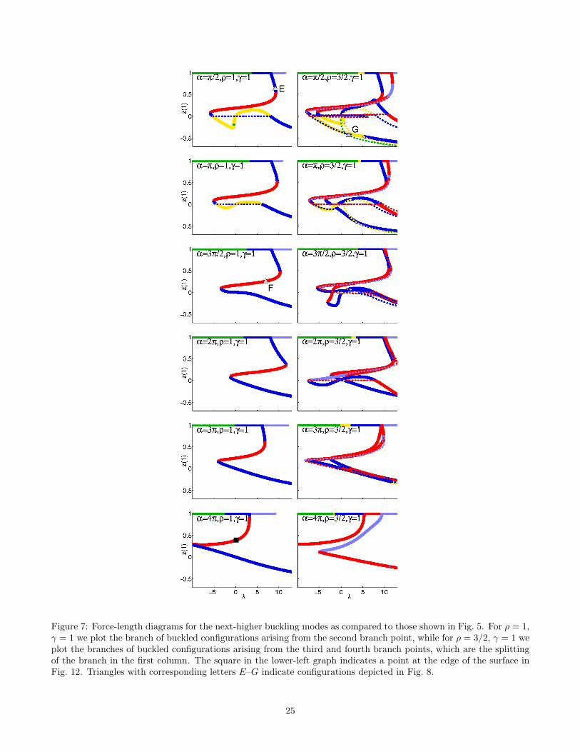
Figure 7: Force-length diagrams for the next-higher buckling modes as compared to those shown in Fig. 5. For ρ = 1,γ = 1 we plot the branch of buckled configurations arising from the second branch point, while for ρ = 3/2, γ = 1 weplot the branches of buckled configurations arising from the third and fourth branch points, which are the splittingof the branch in the first column. The square in the lower-left graph indicates a point at the edge of the surface inFig. 12. Triangles with corresponding letters E–G indicate configurations depicted in Fig. 8.

25

Figure 8: Physical configurations appearing in the bifurcation diagrams in Fig. 7. The centerline of the strut isshown as a green tube, while the director d1 is shown as a blue ribbon.

we are interested in. However, by using a judicious itinerary of parameter switching, one may

compute an approximation of the two-dimensional surface using a collection of one-dimensional

curves [18, 22].

Consider first the computation of the plane of unbuckled equilibria. Of course, the configurations

on this plane are known in closed form, so it is hardly necessary to determine them numerically,

but nevertheless it serves as a useful first example. Furthermore, it is computationally expedient

to compute this plane numerically, since in so doing AUTO will detect branch points to be used as

starting points for the computation of the sheets of buckled equilibria. We begin the computation

of the plane of unbuckled equilibria at (λ, α) = (0, 0). We fix λ = 0, and allow α to vary, giving

a system of the form (25), with α but not λ a component of X. We then perform N steps of

the continuation calculation described in Sec. 7.1, giving a solution branch which we will denote

by (λi,1, αi), 1 ≤ i ≤ N (note that λi,1 = 0 for all i). We now begin a new one-dimensional

continuation calculation at each of the solutions (λi,1, αi) by fixing α = αi and allowing λ to vary.

This leads to a solution branch which we shall denote by (λi,j, αi), 1 ≤ j ≤ M . We choose M to

be fixed for all i so that the result is a “grid” of points in the plane of unbuckled equilibria. Even

though λi,1 = 0 for 1 ≤ i ≤ N , it is not necessarily the case that λi,j = λk,j for j > 1, k 6= i,

since AUTO automatically adapts the step size ∆t during the calculation. We then triangulate

the plane by choosing as the vertices of our triangles (λi,j, αi), (λi+1,j, αi+1), (λi+1,j+1, αi+1) and

(λi,j, αi), (λi,j+1, αi), (λi+1,j+1, αi+1) for 1 ≤ i ≤ N − 1, 1 ≤ j ≤M − 1, as shown in Fig. 9.

The sheets of buckled equilibria are calculated in a similar fashion. During each one-dimensional

continuation in λ on the plane of unbuckled equilibria, AUTO is set to automatically report all

26

λ

α

(λ ,α )

(λ ,α )(λ ,α )

(λ ,α )(λ ,α )1,4 2,4 3,4

1,1 2,1 3,1(λ ,α )1 2 3

1 2 3

Figure 9: Triangulation of plane of unbuckled equilibria: The solid horizontal line at the bottom of the grid represents theinitial calculation fixing λ and allowing α to vary. Each of the solid vertical black lines represents a continuation in λ keepingα fixed. Each (λi,j , αi) is marked with a black circle and the triangulation is shown with the dotted lines.

branch points that it detects. Let λi,1k denote the value of λ at the kth branch point on the branch

with α = αi. We note that, in general, λi,1k 6= λm,1k when m 6= i since the position of the branch

point is a function of α. At each such branch point AUTO can be used to switch branches and

compute a solution branch on the sheet of buckled equilibria emanating from the branch point. So,

similar to the unbuckled case, we have an initial set of solutions (λi,1k , αi) from which we perform

continuation calculations, keeping α fixed and allowing λ to vary. These calculations give rise

to a set of buckled equilibria; we denote the values of λ and α for these equilibria by (λi,jk , αi)

for 1 ≤ i ≤ N and 1 ≤ j ≤ M . Finally, we triangulate the kth sheet by choosing the vertices

of our triangles to be (λi,jk , αi), (λi+1,j

k , αi+1), (λi+1,j+1k , αi+1) and (λi,jk , α

i), (λi,j+1k , αi), (λi+1,j+1

k , αi+1)

for 1 ≤ i ≤ N − 1, 1 ≤ j ≤M − 1, as shown in Fig. 10.

This method for generating bifurcation surfaces is fairly intuitive, but it may not produce smooth

results when the surfaces are complicated, such as the case shown in the second column of Fig. 7.

Folds and sharp bends can be difficult to track smoothly, and because the different one-dimensional

branches are computed independently, the grid may become significantly skewed rather than the

relatively regular cases shown in Figs. 9 and 10. However, if the geometry of the surface is sufficiently

simple, or the discretization is made sufficiently fine, then the surface can be smoothly portrayed.

For example, we now give two examples of the computation of sheets of relatively simple buckled

equilibria. First, we consider the region of the ρ = 1, γ = 1 plane of unbuckled equilibria highlighted

in Fig. 11, and then show in Fig. 12 two sheets of buckled equilibria branching from this region.

Each sheet required approximately 6 hours of computation on a 700 MHz Pentium III Xeon,

and consists of 40 MB of data. For each equilibrium, the index was calculated using a numerical

27

λ

(λ ,α )13,4 3

α

1-z(1)

2,1(λ ,α )

(λ ,α )3,1

(λ ,α )1,1

(λ ,α )1,1

(λ ,α )2,1

(λ ,α )3,1

1,4

(λ ,α )2,4

(λ ,α )3,4

(λ ,α )2,4

(λ ,α )1,4

21

3

2

1(λ ,α )1

31

12

11

1

3

2

1

Figure 10: Triangulation of a sheet of buckled equilibria: As in Fig. 9 the thick black line in the (λ, α) plane represents theinitial continuation in α keeping λ fixed and the thin black lines in the plane represent the continuations in λ keeping α fixed.We now represent the branch points by black squares and show the branches of buckled equilibria emanating from each ofthem. The vertices of the triangulation of the sheet are shown as circles on the branches. This triangulation is indicated bythe dotted lines, although for clarity, we only show the triangulation between the first pair of branches.

implementation of the conjugate point technique discussed in Sec. 2.2 and the surface is color coded

by index, with the color scheme from Fig. 3. The first sheet contains portions of the slices appearing

in column 1 of Fig. 5, while the second sheet matches up with column 1 of Fig. 7. On the first

sheet, buckled solutions very close to the plane of unbuckled equilibria are stable (green) if α is

sufficiently small, but have index 1 (yellow) for larger values of α. Continuing further on the sheet,

we see that the stable equilibria give way to index-1 equilibria as buckling continues. This pattern

is repeated on the second sheet, but with index-2 equilibria giving way to index-3 equilibria.

As a second example, we consider the region of the ρ = 32, γ = 1 plane of unbuckled equilibria

highlighted in Fig. 13, and then show in Fig. 14 two sheets of buckled equilibria branching from

this region. In this case, the sheets of buckled equilibria match up with the slices appearing

in column 2 of Fig. 5, i.e., the splitting of the first sheet of buckled equilibria from the isotropic

problem. The first sheet follows approximately the same pattern of index-0 equilibria giving way

to index-1 equilibria that appeared in the isotropic case, while the second sheet involves a similar

pattern of index-1 equilibria yielding to index-2 equilibria. This pattern is consistent with the usual

expectation for stability of equilibria under symmetry-breaking perturbations: one of the perturbed

images has the index of the symmetric case, and one has index one higher. In addition, we see a

new feature in this case: the presence of an blue (index-2) patch on the first sheet. This blue patch

exists because of a secondary bifurcating sheet, which is not shown in Fig. 14, but can be clearly

seen in the (α = 3π2, ρ = 3

2) slice in Fig. 5, as a yellow dashed branch running on top of a solid blue

branch. The solid blue branch is a slice of the blue patch in Fig. 14, and thus we can infer that

the blue patch is spanned by a nearly parallel yellow patch, of which the yellow dashed branch is a

slice. Looking through the slices in Figs. 5 and 7, we can see that this is the simplest example of

28

Figure 11: A portion of the plane of unbuckled equilibria for an isotropic rod (ρ = 1) with twisting-to-bendingstiffness ratio γ = 1. Within the region marked by the box, we will compute sheets bifurcating from the lines of colorchanges; these sheets are shown in Fig. 12.

the type of surface branching and reconnection that proliferates through the bifurcation surface for

more complicated buckled equilibria, not to mention the dependence of this topological structure

on ρ and γ.

8 Conclusions

In this article, we developed a significant simplification of the standard technique for determining

the index of equilibria in parameter-dependent calculus of variations optimization problems. One

might argue that in practice only local minima are of interest, in which case it would seem more

efficient to employ a minimization algorithm directly, rather than pursue the apparently circuitous

strategy of finding all equilibria and then performing a conjugate point computation to locate the

local minima. For a single optimization problem, this argument may be correct, but for a problem

with one or more parameters, it is less clear. As the parameters are varied, the set of equilibria

tend to form connected sets that are readily tracked by parameter continuation, as we have seen

in the 1-dimensional and 2-dimensional bifurcation diagrams in this paper. In contrast, the local

minima may exist in several disconnected regions of parameter space, more difficult to locate and

track using standard minimization techniques.

29

Figure 12: Portion of the surface of buckled equilibria for an isotropic rod (ρ = 1) with twisting-to-bending stiffnessratio γ = 1, colored by the index of the equilibria according to the color scheme in Fig. 3. For each buckledequilibrium, the value of the force λ, twist angle α, and length z(1) are plotted, and three perspectives of theresulting surface are shown. The plane is the portion of the plane of unbuckled equilibria shown in Fig. 11, and twosheets bifurcate from it. The origin of the red axes is at (α, λ, z(1)) = (0, 0, 1). The spheres and cube correspond tomarked points in the left columns of Figs. 5 and 7.

30

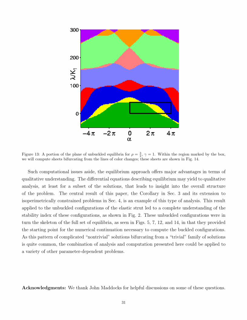
Figure 13: A portion of the plane of unbuckled equilibria for ρ = 32 , γ = 1. Within the region marked by the box,

we will compute sheets bifurcating from the lines of color changes; these sheets are shown in Fig. 14.

Such computational issues aside, the equilibrium approach offers major advantages in terms of

qualitative understanding. The differential equations describing equilibrium may yield to qualitative

analysis, at least for a subset of the solutions, that leads to insight into the overall structure

of the problem. The central result of this paper, the Corollary in Sec. 3 and its extension to

isoperimetrically constrained problems in Sec. 4, is an example of this type of analysis. This result

applied to the unbuckled configurations of the elastic strut led to a complete understanding of the

stability index of these configurations, as shown in Fig. 2. These unbuckled configurations were in

turn the skeleton of the full set of equilibria, as seen in Figs. 5, 7, 12, and 14, in that they provided

the starting point for the numerical continuation necessary to compute the buckled configurations.

As this pattern of complicated “nontrivial” solutions bifurcating from a “trivial” family of solutions

is quite common, the combination of analysis and computation presented here could be applied to

a variety of other parameter-dependent problems.

Acknowledgments: We thank John Maddocks for helpful discussions on some of these questions.

31

Figure 14: Portion of the surface of buckled equilibria for ρ = 32 and with twisting-to-bending stiffness ratio γ = 1,

colored by the index of the equilibria according to the color scheme in Fig. 3. As in Fig. 12, three perspectives ofthe same surface are shown. The plane is the portion of the plane of unbuckled equilibria shown in Fig. 13, and twosheets bifurcate from it. The origin of the red axes is at (α, λ, z(1)) = (0, 0, 1). The spheres and cubes correspond tomarked points in the right column of Fig. 5.

32

Physical configurations and bifurcation surfaces produced in POV-Ray. R.S.M. was supported by

NSF grant DMS-9973258. R.C.P. was supported by NSF grant KDI/NCC Molecular information

and computer modeling in electrophysiology, SBR-9873173.

References

[1] S. S. Antman. Nonlinear Problems of Elasticity. Springer-Verlag, 1995.

[2] O. Bolza. Lectures on the Calculus of Variations. Chelsea Publishing Company, 1973.

[3] A. R. Champneys and J.M.T. Thompson. A multiplicity of localized buckling modes for twisted

rod equations. Proc. R. Soc. Lond. A, 452:2467–2491, 1996.

[4] E. H. Dill. Kirchhoff’s theory of rods. Arch. Hist. Exact Sci., 44:1–23, 1992.

[5] E. J. Doedel, H. B. Keller, and J. P. Kernevez. Numerical analysis and control of bifurcation

problems: (I) Bifurcation in finite dimensions. Int. J. of Bif. and Chaos, 1:493–520, 1991.

[6] E. J. Doedel, H. B. Keller, and J. P. Kernevez. Numerical analysis and control of bifurcation

problems: (II) Bifurcation in infinite dimensions. Int. J. of Bif. and Chaos, 1:745–772, 1991.

[7] G. M. Ewing. Calculus of Variations with Applications. Dover Publications, New York, 1969.

[8] A. Friedman. Foundations of Modern Analysis. Holt, Rinehard & Winston, 1970.

[9] I. M. Gelfand and S. V. Fomin. Calculus of Variations. Prentice-Hall, 1963.

[10] A. Goriely, M. Nizette, and M. Tabor. On the dynamics of elastic strips. Journal of Nonlinear

Science, 11:3–45, 2001.

[11] A.G. Greenhill. Proc. Inst. Mech. Eng., page 182, 1883.

[12] J. Gregory and C. Lin. Constrained Optimization in the Calculus of Variations and Optimal

Control Theory. Van Nostrand Reinhold, New York, 1992.

[13] M. Gutzwiller. Chaos in Classical and Quantum Mechanics. Springer-Verlag, 1990.

[14] M. R. Hestenes. Calculus of Variations and Optimal Control Theory. Robert E. Krieger

Publishing Company, 1966.

[15] H. B. Keller. Numerical solution of bifurcation and nonlinear eigenvalue problems. In P. H.

Rabinowitz, editor, Applications of Bifurcation Theory, pages 359–384. Academic Press, 1977.

[16] G. Kirchhoff. Uber das Gleichgewicht und die Bewegung eines unendlich dunnen elastischen

Stabes. Journal fur die reine und angewandte Mathematik (Crelle), 56:285–313, 1859.

33

[17] A. E. H. Love. A treatise on the mathematical theory of elasticity. Dover, 4th edition, 1927.

[18] J. H. Maddocks, R. S. Manning, R. C. Paffenroth, K. A. Rogers, and J. A. Warner. Interactive

computation, parameter continuation, and visualization. Int. J. of Bif. and Chaos, 7(8):1699–

1715, 1997.

[19] R. S. Manning, K. A. Rogers, and J. H. Maddocks. Isoperimetric conjugate points with appli-

cation to the stability of DNA minicircles. Proc. R. Soc. London A, 454:3047–3074, 1998.

[20] M. Morse. Introduction to Analysis in the Large. Institute for Advanced Study, 1951.

[21] S. Neukirch and M.E. Henderson. Classification of the spatial clamped elastica, parts i and ii.

preprint.

[22] R. C. Paffenroth. Mathematical Visualization, Parameter Continuation, and Steered Compu-

tations. PhD thesis, University of Maryland, College Park, 1999.

[23] M. Renardy and R. Rogers. An Introduction to Partial Differential Equations. Number 13 in

Texts in Applied Mathematics. Springer, 1993.

[24] H. Sagan. Introduction to the Calculus of Variations. Dover Publications, New York, 1969.

[25] M.D. Schuster. A survey of attitude representations. Journal Astronautical Sciences, 41:439–

518, 1994.

[26] G.H.M. van der Heijden, S. Neukirch, V.G.A. Goss, and J.M.T. Thompson. Instability and

self-contact phenomena in the writhing of clamped rods. preprint.

[27] G.H.M. van der Heijden and J.M.T. Thompson. Lock-on to tape-like behaviour in the torsional

buckling of anisotropic rods. Physica D, 112:201–224, 1998.

34