C.P. No. 721

MINISTRY OF AVIATION

AERONAUTICAL RESEARCH COUNCIL

CURRENT PAPERS

Calculation of the Turbulent

Boundary Layer in the Nozzle

of an Intermittent

Axisymmetric Hypersonic Wind Tunnel

BY

N.6. Wood

LONDON: HER MAJESTY’S STATIONERY OFFICE

1964

PRICE 5s. 6d. NET

C.P. No.721

Calculation of' the Turbulent Boundary Layer in the Nozale of an Intermittent Axisymmetric Bypersonic

WindTunnel - By -

N. B. Wood

September. 1963

SLJMMAFLY

An approxknate method of calculating the turbulent boundary layer in a conical nozzle with isothermal wall is described. The morcentum integral technique is used together with a skin-friction coefficient which is assumed to depend on the Reynolds number based on the momentum thichess. Following an analysis by Spence of the experimental data of Lobb, Wink&r and Persh, a l/9 power velocity profde is assumed for the boundary layer and the effect of the transverse curvature of the wall is taken into account. Calculations related to the conditions in the R.A.R.D.E. No.3 Hypersonic Gun Tunnel are presented and the results are compared with experimental pitot-survey data.

Notation

a speed of sound

Cf skin-friction coefficient

H boundary-layer form parameter, S&3

% value of H in incompressible flow

H P

value of H in two-dimensional flow

ii v

M Mach number outside boundary layer

n

p,,b 1

un power of velocity profile, -k = '

ue ( > ;i

ratio of stagnation pressures aoross normal shock

r radial distance from axis of nozzle

R radial distance of nozzle wall from axis

BJ

Replaces A.R.C.25 062

-2-

B*

r UC 8

T

u

A

rl

e

nozzle throat radius

radius of uniform core of flow in nozzle

aistanoe measured along nozcile wall

temperature

longitudinal velocity (without subscript denotes velocity in boundary layer, distance r from axis)

distance measured along nozzle axis

oo-ordinate norm1 to nozzle wall

ratio of specific heats

boundary-layer thickness

boundary-layer displacement thickness,

I 6

transformed boundary-layer thlolmess, e aY Pm 0

transformed co-ordinate normal to wall, I

‘P ay 0 pm

boundary-layer momentum thickness, (5 0 -5) aJ

parameter &fined by equation (17)

visoosity

density

recovery factor, defined by equation (8)

angle between axis and wall of nozzle

Subscripts /

-3-

Subscripts

e conditions at outer edge of boundary layer

m conditions at intermediate temperature, T, iequation (II)]

0 tunnel stagnation conditions

P boundary-layer parameters in two-dimensional flow

T recovery conditions, given by -$ = 1 + _" (Y-l) M 1

2 e

tr

77

parameter transformed according to equation (4)

wall conditions

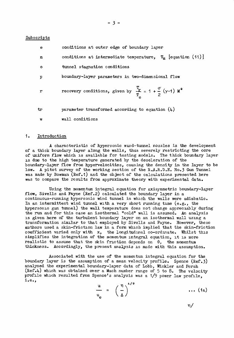
I. Introduction

A characteristic of hypersonic urn&tunnel nozzles is the development of a thick boundary layer along the walls, thus severely restricting the core of uniform flow which 1s available for testing models. The thick boundary layer IS due to the high temperature generated by the deceleration of the boundary-layer flow from hypervelocities, causing the density in the layer to be low. A pitot survey of the workLng section of the B.A.R.D,E. No.3 Gun Tunnel was made by Bowman (Ref.1) and the object of the calculations presented here was to compare the results from approximate theory with experimental data.

Using the momentum integral equation for adsymmetric boundary-layer flow, SivelJx and. Payne (Ref.2) calculated the boundary layer in a continuous-running hypersonic wind tunnel in whxh the walls were adiabatic. In an intermittent wind tunnel with a very short running tzme (e.g., the hypersonzo gun tunnel) the wall temperatunz does not change appreczably during the run and for this case an isothermal "cold" wall is assumed. An analysis IS given here of the turbulent boundary layer on an isothermal wall us=ng a transformation simdar to that employed by Sivells and Payne. However, these authors used a skin-friction law in a form whxh implied that the skin-friction coefficient varied only with x, the longitudinal co-ordmate. Whilst this simplifies the integration of the momentum integral equation, It 1s more realistic to assume that the skin frxtion depends on 0, the momentum thickness. Accordingly, the present analysis IS made with this assumption.

Associated with the use of the momentum integral equation for the boundary layer is the assumption of a mean velocity profile. Spence (Ref.3) analysed. the experimental boundary-layer data of Lobb, Winkler and Persh (Ref.&) whxh was obtained over a Mach number range of 5 to 8. The velocity profde whmlch resulted from Spenoe's analysis was a l/V power la,w profile, i.e.,

iI9

. . . (la)

e

-4-

A = . . . (lb)

In the absence of any other data the above profile has been assumed for the present csloulations.

When the thickness of the boundary layer in adsymmetric flow approaches radius of curvature of the walls the modification of the momentum and displacement effects of the boundary layer must be taken into account and the approach of Miohel (Ref.5) has been followed here.

The botiary layer has been assumed turbulent from the start of the flow since the Reynolds numbers are high throughout (of the order 1 x lOs/ft at the throat).

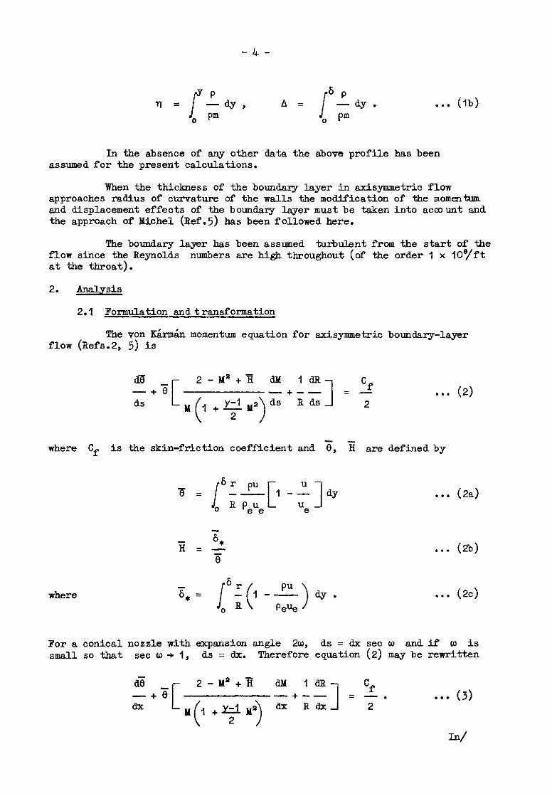
2. Analysis

2.1 Formulation and transformation

The ion K&m&n momentum equation for axisymmetric boundary-layer flow (Refs.2, 5) is

where Cf is the skin-friction coefficient and B, % are defined by

. . . (2a)

. . . (2b)

where T*= [;(1-2-)*. . . . (2c)

For a conical nozzle with expansion angle 20, ds = dx set w and if w is smalls0 that seco+l, ds = ax. Therefore equation (2) may be rewritten

. ..(3)

-5-

In order to simplify the coefficient of dM/d.x, equation (3) is now transformed as follows

. . . (h)

. . . (4b)

i.e., %+I = is;,,+,)L Te

and the following equation is obtained

Y+l

=tr %r dM %r aR 'f Te ---+--(2+Tit,)+--- = - -

ax M ax R ax KI

(y-1 1

. . . . (5) 2 To

'I?le above tl'msformation is similar to the generalisation of the Stewartson- Illingworth transformation, used by Spenoe (Ref.6).

2.2 Evaluation of the form parameter, H

In his analysis of the data of Lobb, Winkler and Persh (Ref.&), Spence (Ref.3) found that the quadratic temperature-velocity relationship was a good approximation to the true variation in the boundary layer. using this relatIonship the two-dimensional form parameter, H

P 1s given by

TW HP+1 =

T, rHi +r.

e * e

For an isothermal wall with temperature T, specified, since

~~,+~M’, equation (6) becomes

-6-

where u is the turbulent wall recovery factor defined by

o- = Tr - Te

To - Te

. . . (7)

l . . (8)

and is observed to be about 0439 for au.

Dividing by To& and usu~g equation (Lb), equation (7) transforms, for y = 1.4, to

TTV 1 + 0.178 MP

%r +I = -II.

P To $+l+0.2Ma ' . . . (9)

The fQRgOiDg relationships apply to two-dimensional boundary layers but it is shown by Muhel (Ref.5) that even for quite large values of 6/R, for a turbulent boundary layer, mp is within a few per cent of unity. Therefore equations (7) and (9) may be used to evaluate 3 and ztr in adsymmetric turbulent boundary layers.

n+2 The incompressible form parameter, Hi is given by Iii = - and n

for n = 9, Hi = II/Y.

2.3 Brpression for the skin friction

The Blasius turbulent skin-friction coefficient, modified for compressibrlity, is (Refs.3,6)

p = ;. c .[pe;fpj3 ‘w

PeUe

and for a I/9 power-law profile tbs becomes

'w 5 Te

z=l-=T e m . . . (IO)

since pressure is constant acrc~ss the boundary layer, sothat L$. Pe m

Once/

Once again and writing equation parameters gives

-7-

this formula IS for two-dimensional boundary (10) XII terms of sxxgmaetr~c boundary-layer

layers

. . . (108)

for a l/y power-law velocity profile and small W. The last two terms in equation (lOa) are close to unity and writing it in terms of the transformed momentum thickness lead8 to

2 = 0.0088 Te Te ;[-,*[ v.::4, ji . . . . (lob)

2

2.4 The intermediate temperature, T,, and calculation of viscosity, h

The commonly used definition of the Lntermediate or reference temperature T, is that due to Eckert (Ref.7) and is

Tm = O-5 (Tw + T,) + 0.22 (Tr - Te) . . . . (Ila)

For an isothermal wall, Tw is specified and T, is written in the form

T 2

T = O-5 (1 + O-078 Ma) + O-5 J! (1 + 0.2 MP)

Te TO

for air with y = l-4, o- = 0.89.

. . . (llb)

The viscosity, p, may be calculated from Southerland's law whioh is, for air, with T in OK,

-a-

T=‘=X 3.059 x I@ P = . . . (12)

T + 114

measured in slug/f+" sec. There is no need to introduce .a simpler approximate relation when integrating numerically on an electronic digital computer, as has been done here.

2.5 Inteaation of the momentum equation

From equations (5) and (lob) the momentum equation may be written

. . . (13)

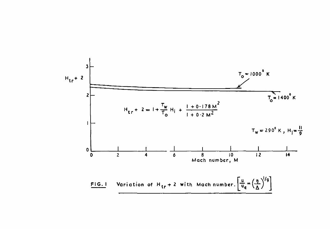
If both sides of equation (11) are now multiplied by iz't,

the left-hand side of the equation becomes a perfect differential Ff Htr + 2

can be assumed constant. over the interval of integration. Fig.1 shows the variation of I-& + 2 with M and demonstrates that this is a reasonable assumption. Therefore equation (II) simplFfies to

The parameters in the above equation are functions of Mach number M and so it is simpler to integrate w.r.t.M. The one-dimensional theory for the UnifcIm core gives

. . . (15)

from which

-P- 5-3Y

4(Y-1) - CM2 - 4) fl +y-lbA

al db, R, 1 . '\ 2 / --- =- - ald aM J 2 M3 Y+l

/ y+l \4(y-')

. . . (16a)

\2/

and since aR -=tanO=‘, aoJ

equation (16a) becomes

5-JY

4(Y-1) (MD - ah, d4

.d.M+-.-. Y+l

. . . (16b) aM 0

( y+l p-1)

\ 2 /

Substituting equation

-i

(16b) in equation (13) and since

i (1 + 0.2 ?dq (PO&O)

M ?

for y = 1.4, equation (13) becomes

R* I (2 - I)(1 + 0.2 lb+ as

[$ x - - +* ahi. ..* (17) 2 II' (1'2)$ dY 1

Since the geometry of the conical expansion has been included in equation (17), the equation is only valid for the supersonic re&on downstream of the throat and so the limits of integration are a = 1, b = Mn. using a similar expression applied to the subsonio contraction an estimate may be made of the bodary-layer thickness at the throat.

With/

- IO -

With equations (lib) and (12) substituted into equation (17), the latter may be integrated numerically to obtain $.

since 6, and 2% dM

are not initially known, it is necessary to

assume that they are eem initially and then by iteration a true solution can be obtsified.

2.6 Calculation of the boundary-layer thicknesses

To obtain z from $, equation (&a) and (15) are substituted into the left-hand side of equation (17) to give

= s . . . (18) 1 + 0.2 Ma 3 1 t6, Y Htr+2

l-2

evaluated at M = M,(x) .

The value of 6, is given by (under the assumptions made in $2.2)

x* = Hi = < >. (1 t 0.2 Ma) Hi t O-178 MP 1 . . . . (19)

The true momentum and displacement thicknesses, 0 and 6*, are obtained from the expressions (Ref.8)

T;, = 6, - s”, 2 * .

. . . (20)

It may not be possible to allow for the variation of K with pressure gradient in the present application without making wildly speculative ~SSUIOP~~OIIS (Ref.6), but for most purposes Hi can be assumed to remain constant (Refs.6,8) and in particular for a l/Y power velocity profile, Hi = II/Y.

From/

- 11 -

From equations (1) and the definitions of the momentum and dxplacement thicknesses, which are

. . . (21)

it can be shown that for (;) = (;j, the thxkness of the boundary

layer 6 1s

. . . (22)

It will be seen from equation (19) that as M becomes large H also becomes large. Thus, at high Mach number 6, is of the same order as 6 whereas 0 is a smaller fraction of 6 compared with the value at low Mach numbers. This 1s because the gas in most of the boundary lsyer is much hotter than in the uniform core and so the density is lower. Thus, in equations (21)

the term z is small in comparison with unity across most of the layer. Pe"e

3. Results

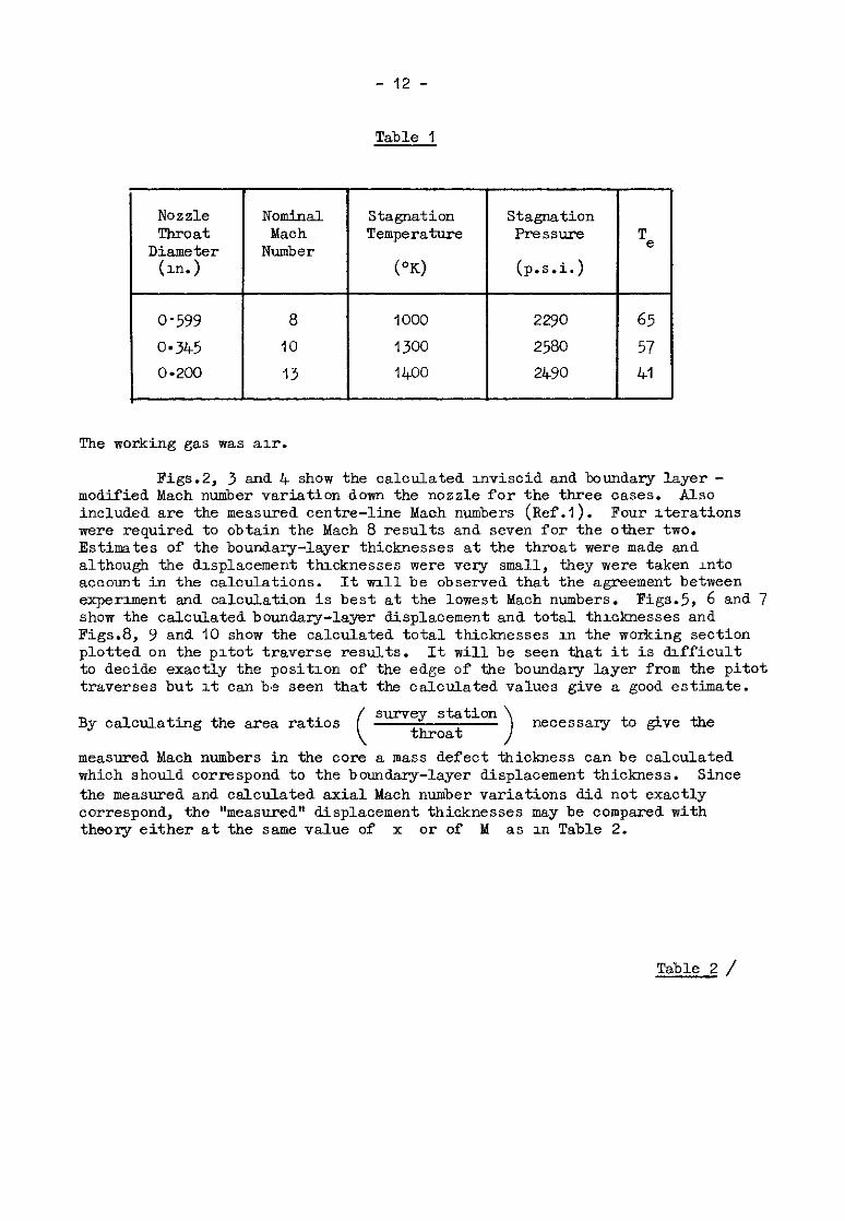
Equation (17) was integrated numerically with the ad of an electronic digital computer AMOS (Ferranti Mark I*), using a I6 point Gauss quadrature formula, for the co&Ci.tions in the naszle of the B.A.R.D.E. 10 inch hypersonic gun tunnel. The tunnel has a conical nozzle with a 4" semi-angle and the Mach number is varied by mterchangeable throat inserts. The conditions considered were as follows:

Table I/

- 12 -

Table 1

Nozzle Nozzle Throat Throat

Diameter Diameter c-1 c-1

o-599 o-599

0.345 0.345

0.200 0.200

Noloinal Nominal Mach Mach

Number Number

8 8

10 10

13 13

Stagnation Stagnation Temperature Temperature

(OK) (OK)

1000 1000

1300 1300

1400 1400

stagnation Stagnation Pressure Pressure

(p.s.i.) (p.s.i.)

2290 2290

2580 2580

2490 2490

Te Te

65 65

57 57

41 41

The working gas was az.

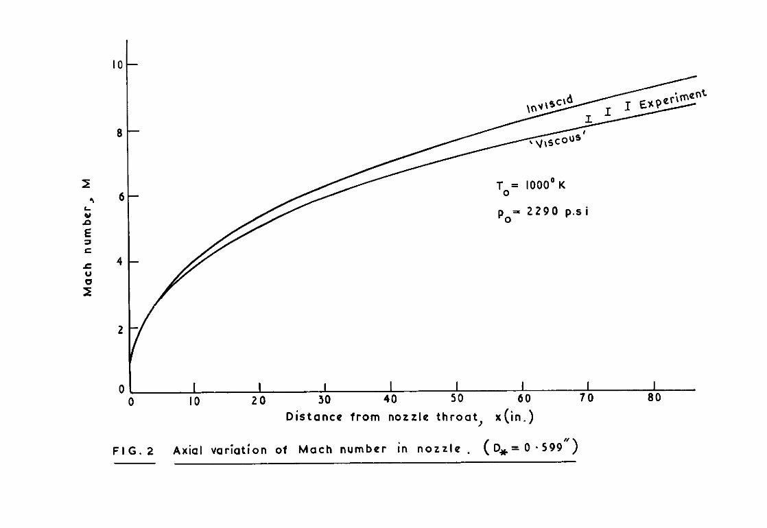
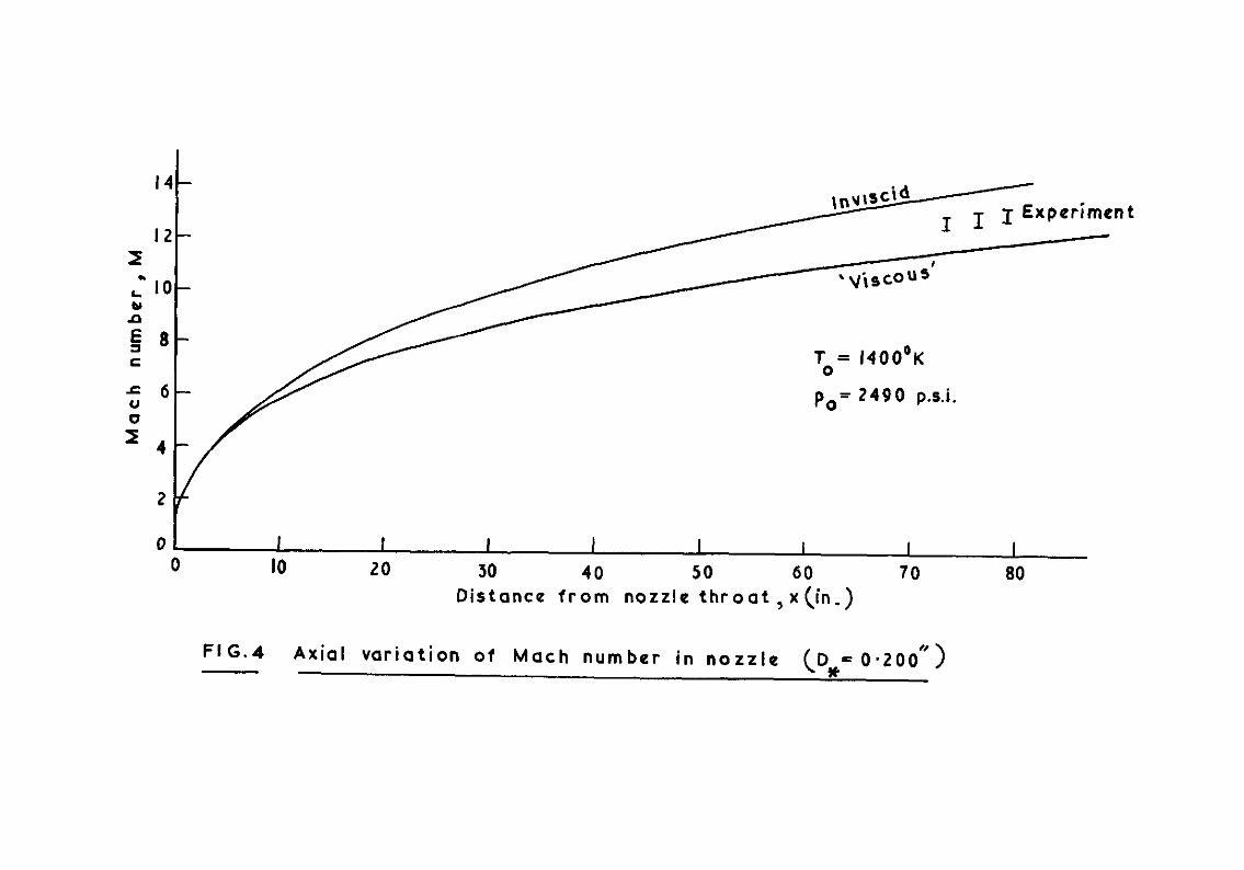
Figs.2, 3 and 4 show the caloulated Inviscid and boundary layer - modified Mach number variation down the nozzle for the three oases. Also included are the measured centre-line Mach numbers (Xef.1). Four rterations were required to obtain the Mach 8 results and seven for the other two. Estimates of the boundary-layer thicknesses at the throat were made and although the displacement thcknesses were very small, they were taken Into account in the calculations. It ~~11 be observed that the agreement between experiment and. calculation is best at the lowest Mach numbers. Figs.5, 6 and 7 show the calculated boundary-layer displacement and total thicknesses and Figs.8, 9 and 10 show the calculated total thicknesses m the working section plotted on the pItot traverse results. It will be seen that it is difficult to decide exactly the positlon of the edge of the boundary layer from the pitot traverses but It can bcz seen that the calculated values give a good estimate.

By calculating the area ratios (

survey station throat >

necessary to give the

measured Mach numbers in the core a mass defect thickness can be calculated which should correspond to the boundary-layer displacement thickness. Since the measured and calculated axial Mach number variations did not exactly correspond, the "measured" displacement thicknesses may be compared with theory either at the same value of x or of M as XI Table 2.

Table 2 /

- 13 -

Table 2

Throat s* Calculated 6* Diameter

(3.n.) M (CL) Tz"j M (co1.2) ' x (co1.3)

a .3 70.2 Q '74 I *OQ 0.94 0.599 8.5 73.2 0.72 1 *IO 1 -co

a-7 76.2 0.66 1.20 I.07

10.2 72.1 144 1.70 I.43 0.345 20.4 75.1 0.99 I.82 I.51

10.7 78-l 0.95 2 -04 I -60

12.7 :6": -

l-12 2.86 1.98 0.200 12.9 1.22 j-00 2 *IO

13.0 79-2 1.31 399 2.22

The analysis by Spence of the data of Lobb et al has already been mentioned as the basis of the theory used here. The expression for the form parameter H iequation (6)j has b een based on the fact that the quadratic temperature-velocity relatlonslp appeared to hold. However, if the measured value of 6,/e from Ref.4 1s compared with that calculated from equation (6) there is a strong disagreement as shown in Table 3.

Table 3

493 5.42 Il.42 IO.96

5-75 6.19 12.92 13.45

6.83 6.34 13.92 16.05

7-67 5.94 12.47 17.73

8.18 6.60 11'52 19.97

- 14 -

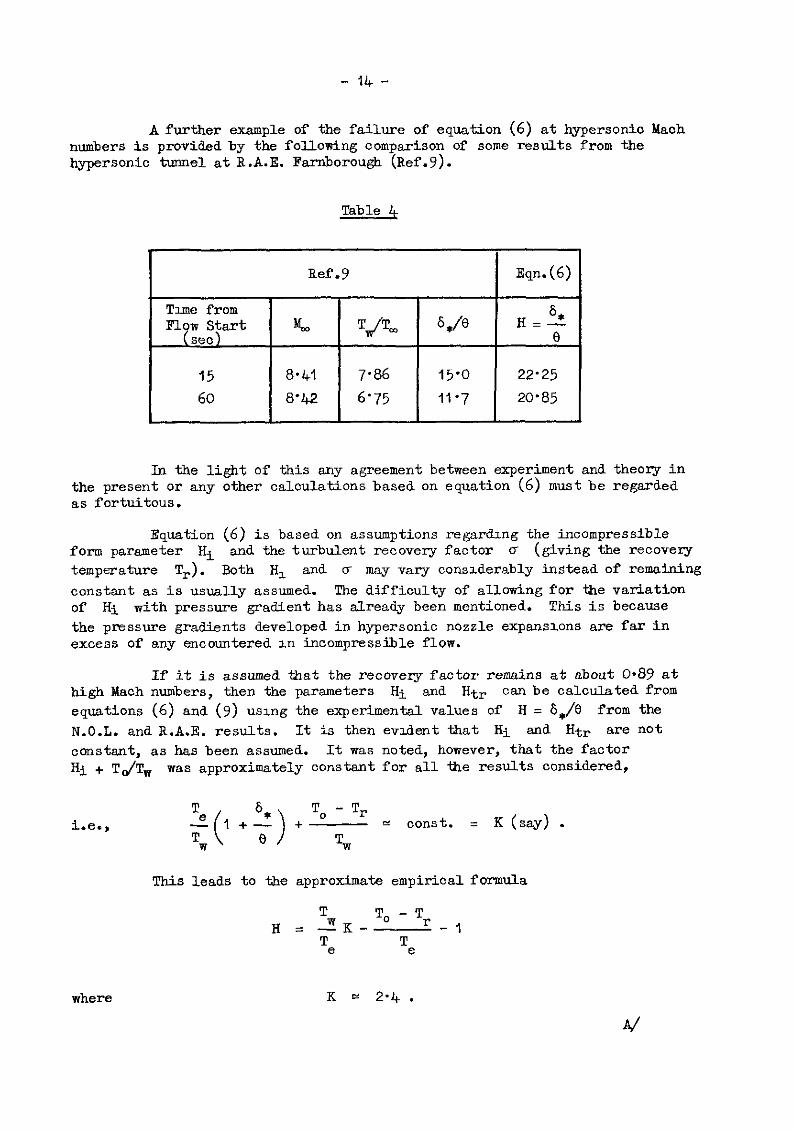
A further example of the failure of equation (6) at hypersonic Mach numbers is provided by the following comparison of some results from the hypersonic tunnel atR.A.E. Farnborough (Ref.9).

Table 4

Ref.9 I Eqn. (6)

7.86 15'0 22'25

6’75 11'7 20'85

In the light of this any agreement between experiment and theory in the present or any other calculations based on equation (6) must be regarded as fortuitous.

Equation (6) is based on assumptions regar&ng the incompressible form parameter Hi and the turbulent recovery factor c (giving the recovery temperature T,). Both Hz and IS may vary consIderably instead of remaining constant as is usually assumed. The difficulty of allowing for the variation of Hi with pressure gradient has already been mentioned. This is because the pressure gradients developed in hypersonic nozzle expansxons are far in excess of any encountered in incompressible flow.

If it is assumed that the recovery factor remains at about O-89 at high Mach numbers, then the parameters Hi and Htr can be calculated from equations (6) and (9) usmg the experimental values of H = S,/e from the N.O.L. and R.A.E. results. It is then evident that Hi and Htr are not constant, as has been assumed. It was noted, however, that the factor Hi + TdT, was approximately constant for all the results considered,

i.e., To - ‘Jr e const. = K (say) .

Tw

This leads to the approximate empirical formula

T H = J!K- To - Tr

- 1 Te Te

where K * 2-4 .

- 15 -

A simpler empirical formla was noted by Lee (Eef.10). !l'his was

and in fact the N.O.L. and R.A.E. results are all near this figure, the arithmetical mean being 2.4.

However, it is clearly most unsatisfactory to propose empirical. laws of this kind, with no theoretical backmg, and it is plain that there is considerable scope for both theoretical and experimental research to improve our knowledge of turbulent boundary layers in hypersonic flow.

4. Conclusions

The turbulent boundary layer in the nozzle of the R.A.R.D.E. IO in. gun tunnel has been calculated using the momentum equation and an assumed power-law profile based on experimental observations. Good agreement between theory and experiment was obtained for the total boundary-layer thiclmess but because of discrepancies in the theory this is regarded as fortuitous. There was a definite inconsistency between the experimentaIL and calculated boundary-layer displacement thicknesses.

In order to design hgh Reynolds number hypersonic wind keels with confidence, there is a need for more experimental and theoreticd research in turbulent hypersomc boundary lsyers.

References /

- 16 -

References

&.

I

2

3

Author(s) Title, etc.

J. E. Bowman Unpublished War Office Memo. 1962.

J. C. Sivells and

R. G. Payne

A method of calculating turbulent boundary layer growth at hypersonic Mach numbers. AEDC-'E-59-3, March, 1959.

D. A. Spence

4 R. K. Lobb, E. M. Winkler

and J. Persh

5 R. Michel

6 D. A. Spenoe

7 E. R. G. Eokert

8 E. C. Maskell

9 J. F. W. Crane

10 J. D. Lee

Velocity and enthalpy distributions in the compressible turbulent boundary lsyer on a flat plate. Journal of Fluid Mechanics, Vo1.8, No.3, 1960.

N.O.L. Hypersonic TunnelNo.4. Results VII: Experimental mvestrgation of turbulent boundary layers in hypersonic flow. NavOrd Report 3880, March, 1955,

Developpement de la couche limite dans une tuyere hypersonlque. AGARIJ Specialxts' Meeting "High temperature aspects of hypersonic flow". Rhode-Saint-Genese, Belgium, Aprd, 1962.

The growth of compressible turbulent boundary layers on isothermal and adiabatic walls. A.R.C. R.& M.3191. June, 1959.

Engineering relations for friction and heat transfer in high velocity flow. J. Aero. Sci., Vo1.22, No.8, August, 1955.

Approxmate calculation of the turbulent boundary layer m two-&mensional compressible flow. Unpublished M.O.A. Report.

Private communication.

Axisymetric nozzles for hypersonic flows. Ohzo State University Research Foundation, TN ALOSU 459-1, 1959.

Htr+ *

2

I

0

To= 1000’ K

n

Htr+ 2P TW

I+- Hi + 0

0 I 2

I 4 6

I I 0 IO

Mach number, M

I I I2 14

To- 1400” K

I +0.178M2

I t 0*2M2

T, = 290’ K, Hi=+

FIG. I Variatton of Htr + 2 with Mach number.

6 p,= 2290 p.si

I IO

I I I I I I I 20 30 40 50 60 70 80

Distance from nozzle throat, x(in.)

FIG. 2 Axial variation of Mach number in nozzle . (D,=O-599")

To= lJOO” K

PO= 2580 pd.

I IO

I I I I 20

I SO 40

I I

Distance from nozzle tSh:oat (in .;” 70 80

FIG. 3 Axial variation of Mach number in nozzle (OS= O*345”)

14-

To= 1400'K

po= 2490 p.s.i.

I IO

I I I I I I I 20 30 40 50 60 70 80

Distance from nozzle throat ,x(in.)

FIG.4 Axial variation of Mach number in nozzle (De= 0*20011 >

20 30 40 50 60 70 80 90

Distance from nozzle throat, x (in .)

FIG.5 Calculated boundary-layer growth in Mach 8 nozzle.

x 0

:. I

Distance trom nozzle throat, x (in.)

FIG 6 Calculated boundary-layer growth in Mach IO nozzle.

5 4 I

20 30 40 50 Distanca from nozzle throat, x (in.)

FIG. 7 Calculatad boundary-layer growth in Mach 13 nozzle

6

x =7OI22”

‘UC

i’l- x = 73.2”

x ~76.2”

4

t I I I

7.0 6-5 6-O I lO-3

Normal shack stagnation pressure ratio

F&J. Comparison of calculated uniform core

with experimental pitot traverses. D& =

Mach 8 throat.

Nozzle wall

\\\\\““” \\\\\’

Calculated edge ___--.---

ryer ---

x=72*1” h - . x 78 I” 5 -

I I I 2.8

I 2.6 2-4 2-2 x w3

Normal shock stagnation pressure rotio po2/ POI

FIG .9 Comparison of calculated uniform core radius (ruE) with experimental pitot traverses. 0, c 0.345’3

(Mach IO throat3

U- U- Noz 210 Wd NOZ 210 wd \\ \\U”“’ \\ \\U”“’

W------- W------- S- S-

4- 4-

~~79.2”

4 t

I I I I *OS

I I.00 0.95 0.90 x lo- 3

Normal shock stagnation pressure ratio p021Po,

flG.10 Comparison of calculated uniform core radius &,c)

with experimental pitot traverses

(Mach 13 throat)

.(v, = 0.200’~

C.P. No. 721

0 Crow copyrrght 1964

Prmted and pubbshed by

HER MAJESTY’S STATIONERY OFFICE

To be purchased from York House, Kmgsway, London w c.2

423 Oxford Street, London w 1 13.4 Castle Street, Eidmburgh 2

109 St Mary Street, Cardiff 39 Kmg Street, Manchester 2

50 Fanfax Street, Bristol 1 35 Smallbrook, IQngway, B~rmn&am 5

80 Cluchester Stmt, Belfast 1 or through any bookseIIer

Printed zn England

C.P. No. 721 S.0. Code No. 23-9015-21