calculus (lebih kearah fisika)
TRANSCRIPT
1

2

3

4
Light and Matter
Fullerton, Californiawww.lightandmatter.com
copyright 2005 Benjamin Crowell
rev. April 26, 2008
This book is licensed under the Creative Com-mons Attribution-ShareAlike license, version 1.0,http://creativecommons.org/licenses/by-sa/1.0/, exceptfor those photographs and drawings of which I am notthe author, as listed in the photo credits. If you agreeto the license, it grants you certain privileges that youwould not otherwise have, such as the right to copy thebook, or download the digital version free of charge fromwww.lightandmatter.com. At your option, you may also copythis book under the GNU Free Documentation License version1.2, http://www.gnu.org/licenses/fdl.txt, with no invariantsections, no front-cover texts, and no back-cover texts.

5
1 Rates of Change1.1 Change in discrete steps 9
Two sides of the same coin,9.—Some guesses, 11.
1.2 Continuous change . . 12A derivative, 14.—Propertiesof the derivative, 15.—Higher-order polynomials,16.—The second derivative,16.—Maxima and minima,18.
Problems. . . . . . . . 21
2 To infinity — andbeyond!2.1 Infinitesimals. . . . . 232.2 Safe use of infinitesimals 262.3 The product rule . . . 302.4 The chain rule . . . . 332.5 Exponentials andlogarithms . . . . . . . 34
The exponential, 34.—Thelogarithm, 36.
2.6 Quotients . . . . . . 372.7 Differentiation on acomputer . . . . . . . . 382.8 Continuity . . . . . . 412.9 Limits . . . . . . . 42
L’Hopital’s rule, 45.—Another perspective on inde-terminate forms, 47.—Limitsat infinity, 48.
Problems. . . . . . . . 50
3 Integration3.1 Definite and indefiniteintegrals . . . . . . . . 553.2 The fundamental theoremof calculus . . . . . . . 583.3 Properties of the integral 59
3.4 Applications . . . . . 60Averages, 60.—Work, 61.—Probability, 61.
Problems. . . . . . . . 67
4 Techniques4.1 Newton’s method . . . 694.2 Implicit differentiation . 704.3 Taylor series . . . . . 714.4 Methods of integration . 76
Change of variable, 76.—Integration by parts, 78.—Partial fractions, 79.
Problems. . . . . . . . 83
5 Complex numbertechniques5.1 Review of complexnumbers . . . . . . . . 855.2 Euler’s formula . . . . 885.3 Partial fractions revisited 90Problems. . . . . . . . 91
6 Improper integrals6.1 Integrating a function thatblows up . . . . . . . . 936.2 Limits of integration atinfinity . . . . . . . . . 94Problems. . . . . . . . 96
7 Iterated integrals7.1 Integrals inside integrals 977.2 Applications . . . . . 997.3 Polar coordinates . . . 1017.4 Spherical and cylindricalcoordinates . . . . . . . 102Problems. . . . . . . . 104
A Detours 107
6
B Answers and solutions115
C Photo Credits 133
D Reference 135D.1 Review . . . . . . . 135
Algebra, 135.—Geometry,
area, and volume, 135.—Trigonometry with a righttriangle, 135.—Trigonometrywith any triangle, 135.
D.2 Hyperbolic functions. . 135D.3 Calculus . . . . . . 136
Rules for differentiation,136.—Integral calculus,136.—Table of integrals, 136.

7
PrefaceCalculus isn’t a hard subject.
Algebra is hard. I still remem-ber my encounter with algebra. Itwas my first taste of abstraction inmathematics, and it gave me quitea few black eyes and bloody noses.
Geometry is hard. For most peo-ple, geometry is the first time theyhave to do proofs using formal, ax-iomatic reasoning.
I teach physics for a living. Physicsis hard. There’s a reason that peo-ple believed Aristotle’s bogus ver-sion of physics for centuries: it’sbecause the real laws of physics arecounterintuitive.
Calculus, on the other hand, is avery straightforward subject thatrewards intuition, and can be eas-ily visualized. Silvanus Thompson,author of one of the most popularcalculus texts ever written, opinedthat “considering how many foolscan calculate, it is surprising thatit should be thought either a diffi-cult or a tedious task for any otherfool to master the same tricks.”
Since I don’t teach calculus, I can’trequire anyone to read this book.For that reason, I’ve written it sothat you can go through it andget to the dessert course with-out having to eat too many Brus-sels sprouts and Lima beans alongthe way. The development of anymathematical subject involves alarge number of boring details thathave little to do with the main
thrust of the topic. These detailsI’ve relegated to a chapter in theback of the book, and the readerwho has an interest in mathemat-ics as a career — or who enjoys anice heavy pot roast before movingon to dessert — will want to readthose details when the main textsuggests the possibility of a detour.

8
1 Rates of Change1.1 Change in
discrete stepsToward the end of the eighteenthcentury, a German elementaryschool teacher decided to keep hispupils busy by assigning them along, boring arithmetic problem.To oversimplify a little bit (whichis what textbook authors alwaysdo when they tell you about his-tory), I’ll say that the assignmentwas to add up all the numbersfrom one to a hundred. The chil-dren set to work on their slates,and the teacher lit his pipe, con-fident of a long break. But al-most immediately, a boy namedCarl Friedrich Gauss brought uphis answer: 5,050.
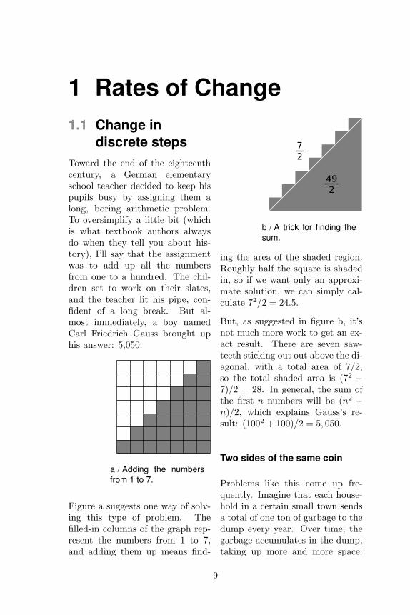
a / Adding the numbersfrom 1 to 7.
Figure a suggests one way of solv-ing this type of problem. Thefilled-in columns of the graph rep-resent the numbers from 1 to 7,and adding them up means find-
b / A trick for finding thesum.
ing the area of the shaded region.Roughly half the square is shadedin, so if we want only an approxi-mate solution, we can simply cal-culate 72/2 = 24.5.
But, as suggested in figure b, it’snot much more work to get an ex-act result. There are seven saw-teeth sticking out out above the di-agonal, with a total area of 7/2,so the total shaded area is (72 +7)/2 = 28. In general, the sum ofthe first n numbers will be (n2 +n)/2, which explains Gauss’s re-sult: (1002 + 100)/2 = 5, 050.
Two sides of the same coin
Problems like this come up fre-quently. Imagine that each house-hold in a certain small town sendsa total of one ton of garbage to thedump every year. Over time, thegarbage accumulates in the dump,taking up more and more space.
9

10 CHAPTER 1. RATES OF CHANGE
c / Carl Friedrich Gauss(1777-1855), a long timeafter graduating from ele-mentary school.
Let’s label the years as n = 1, 2,3, . . ., and let the function1 x(n)represent the amount of garbagethat has accumulated by the endof year n. If the population isconstant, say 13 households, thengarbage accumulates at a constantrate, and we have x(n) = 13n.
But maybe the town’s populationis growing. If the population startsout as 1 household in year 1, andthen grows to 2 in year 2, and soon, then we have the same kindof problem that the young Gausssolved. After 100 years, the accu-mulated amount of garbage will be5,050 tons. The pile of refuse growsmore and more every year; the rateof change of x is not constant. Tab-ulating the examples we’ve done sofar, we have this:
1Recall that when x is a function, thenotation x(n) means the output of thefunction when the input is n. It doesn’trepresent multiplication of a number x bya number n.
rate of change accumulatedresult
13 13nn (n2 + n)/2
The rate of change of the functionx can be notated as x. Given thefunction x, we can always deter-mine the function x for any valueof n by doing a running sum.
Likewise, if we know x, we can de-termine x by subtraction. In theexample where x = 13n, we canfind x = x(n) − x(n − 1) = 13n −13(n − 1) = 13. Or if we knewthat the accumulated amount ofgarbage was given by (n2 + n)/2,we could calculate the town’s pop-ulation like this:
n2 + n
2− (n− 1)2 + (n− 1)
2
=n2 + n−
(n2 + 2n− 1− n+ 1
)2
= n
d / x is the slope of x .
The graphical interpretation of
1.1. CHANGE IN DISCRETE STEPS 11
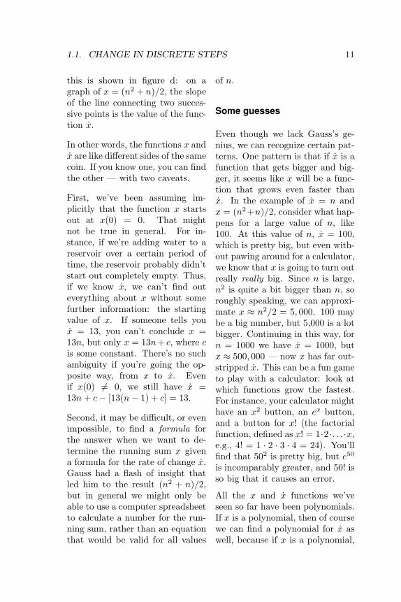
this is shown in figure d: on agraph of x = (n2 + n)/2, the slopeof the line connecting two succes-sive points is the value of the func-tion x.
In other words, the functions x andx are like different sides of the samecoin. If you know one, you can findthe other — with two caveats.
First, we’ve been assuming im-plicitly that the function x startsout at x(0) = 0. That mightnot be true in general. For in-stance, if we’re adding water to areservoir over a certain period oftime, the reservoir probably didn’tstart out completely empty. Thus,if we know x, we can’t find outeverything about x without somefurther information: the startingvalue of x. If someone tells youx = 13, you can’t conclude x =13n, but only x = 13n+ c, where cis some constant. There’s no suchambiguity if you’re going the op-posite way, from x to x. Evenif x(0) 6= 0, we still have x =13n+ c− [13(n− 1) + c] = 13.
Second, it may be difficult, or evenimpossible, to find a formula forthe answer when we want to de-termine the running sum x givena formula for the rate of change x.Gauss had a flash of insight thatled him to the result (n2 + n)/2,but in general we might only beable to use a computer spreadsheetto calculate a number for the run-ning sum, rather than an equationthat would be valid for all values
of n.
Some guesses
Even though we lack Gauss’s ge-nius, we can recognize certain pat-terns. One pattern is that if x is afunction that gets bigger and big-ger, it seems like x will be a func-tion that grows even faster thanx. In the example of x = n andx = (n2 +n)/2, consider what hap-pens for a large value of n, like100. At this value of n, x = 100,which is pretty big, but even with-out pawing around for a calculator,we know that x is going to turn outreally really big. Since n is large,n2 is quite a bit bigger than n, soroughly speaking, we can approxi-mate x ≈ n2/2 = 5, 000. 100 maybe a big number, but 5,000 is a lotbigger. Continuing in this way, forn = 1000 we have x = 1000, butx ≈ 500, 000 — now x has far out-stripped x. This can be a fun gameto play with a calculator: look atwhich functions grow the fastest.For instance, your calculator mighthave an x2 button, an ex button,and a button for x! (the factorialfunction, defined as x! = 1·2·. . .·x,e.g., 4! = 1 · 2 · 3 · 4 = 24). You’llfind that 502 is pretty big, but e50
is incomparably greater, and 50! isso big that it causes an error.
All the x and x functions we’veseen so far have been polynomials.If x is a polynomial, then of coursewe can find a polynomial for x aswell, because if x is a polynomial,
12 CHAPTER 1. RATES OF CHANGE
then x(n)−x(n−1) will be one too.It also looks like every polynomialwe could choose for x might alsocorrespond to an x that’s a poly-nomial. And not only that, but itlooks as though there’s a patternin the power of n. Suppose x is apolynomial, and the highest powerof n it contains is a certain num-ber — the “order” of the polyno-mial. Then x is a polynomial ofthat order minus one. Again, it’sfairly easy to prove this going oneway, passing from x to x, but moredifficult to prove the opposite rela-tionship: that if x is a polynomialof a certain order, then x must bea polynomial with an order that’sgreater by one.
We’d imagine, then, that the run-ning sum of x = n2 would be apolynomial of order 3. If we cal-culate x(100) = 12 + 22 + . . . +1002 on a computer spreadsheet,we get 338,350, which looks sus-piciously close to 1, 000, 000/3. Itlooks like x(n) = n3/3 + . . ., wherethe dots represent terms involvinglower powers of n such as n2.
1.2 Continuouschange
Did you notice that I sneakedsomething past you in the exampleof water filling up a reservoir? Thex and x functions I’ve been usingas examples have all been functionsdefined on the integers, so theyrepresent change that happens indiscrete steps, but the flow of water
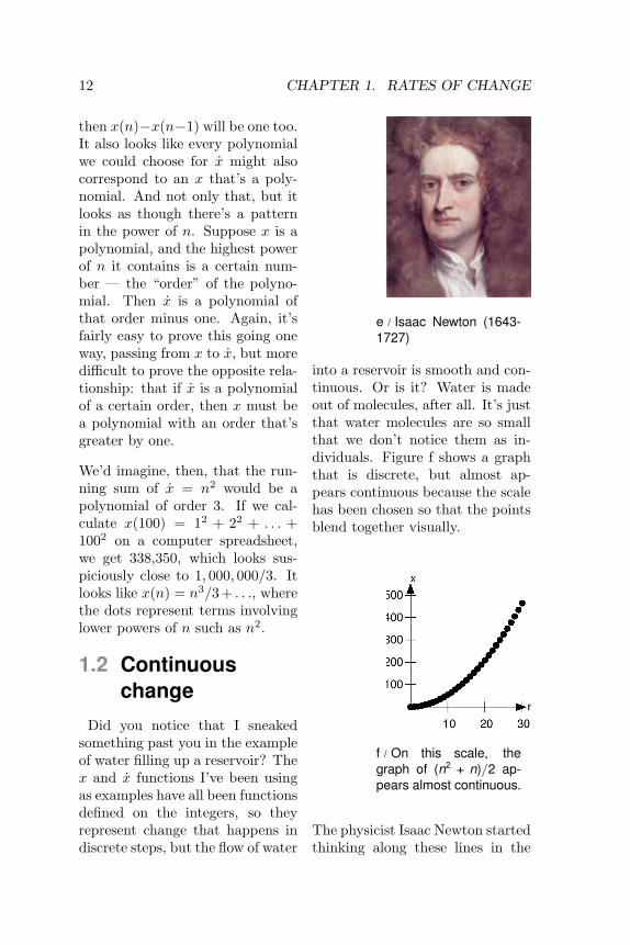
e / Isaac Newton (1643-1727)
into a reservoir is smooth and con-tinuous. Or is it? Water is madeout of molecules, after all. It’s justthat water molecules are so smallthat we don’t notice them as in-dividuals. Figure f shows a graphthat is discrete, but almost ap-pears continuous because the scalehas been chosen so that the pointsblend together visually.
f / On this scale, thegraph of (n2 + n)/2 ap-pears almost continuous.
The physicist Isaac Newton startedthinking along these lines in the
1.2. CONTINUOUS CHANGE 13
1660’s, and figured out ways of an-alyzing x and x functions that weretruly continuous. The notation xis due to him (and he only used itfor continuous functions). Becausehe was dealing with the continuousflow of change, he called his newset of mathematical techniques themethod of fluxions, but nowadaysit’s known as the calculus.
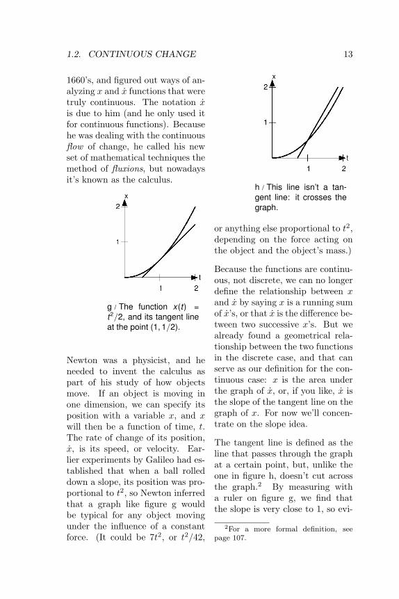
g / The function x(t) =t2/2, and its tangent lineat the point (1, 1/2).
Newton was a physicist, and heneeded to invent the calculus aspart of his study of how objectsmove. If an object is moving inone dimension, we can specify itsposition with a variable x, and xwill then be a function of time, t.The rate of change of its position,x, is its speed, or velocity. Ear-lier experiments by Galileo had es-tablished that when a ball rolleddown a slope, its position was pro-portional to t2, so Newton inferredthat a graph like figure g wouldbe typical for any object movingunder the influence of a constantforce. (It could be 7t2, or t2/42,
h / This line isn’t a tan-gent line: it crosses thegraph.
or anything else proportional to t2,depending on the force acting onthe object and the object’s mass.)
Because the functions are continu-ous, not discrete, we can no longerdefine the relationship between xand x by saying x is a running sumof x’s, or that x is the difference be-tween two successive x’s. But wealready found a geometrical rela-tionship between the two functionsin the discrete case, and that canserve as our definition for the con-tinuous case: x is the area underthe graph of x, or, if you like, x isthe slope of the tangent line on thegraph of x. For now we’ll concen-trate on the slope idea.
The tangent line is defined as theline that passes through the graphat a certain point, but, unlike theone in figure h, doesn’t cut acrossthe graph.2 By measuring witha ruler on figure g, we find thatthe slope is very close to 1, so evi-
2For a more formal definition, seepage 107.

14 CHAPTER 1. RATES OF CHANGE
dently x(1) = 1. To prove this, weconstruct the function representingthe line: `(t) = t − 1/2. We wantto prove that this line doesn’t crossthe graph of x(t) = t2/2. The dif-ference between the two functions,x− `, is the polynomial t2/2− t+1/2, and this polynomial will bezero for any value of t where theline touches or crosses the curve.We can use the quadratic formulato find these points, and the resultis that there is only one of them,which is t = 1. Since x− ` is posi-tive for at least some points to theleft and right of t = 1, and it onlyequals zero at t = 1, it must neverbe negative, which means that theline always lies below the curve,never crossing it.
A derivative
That proves that x(1) = 1, but itwas a lot of work, and we don’twant to do that much work to eval-uate x at every value of t. There’sa way to avoid all that, and find aformula for x. Compare figures gand i. They’re both graphs of thesame function, and they both lookthe same. What’s different? Theonly difference is the scales: in fig-ure i, the t axis has been shrunkby a factor of 2, and the x axis bya factor of 4. The graph looks thesame, because doubling t quadru-ples t2/2. The tangent line hereis the tangent line at t = 2, nott = 1, and although it looks likethe same line as the one in figure
g, it isn’t, because the scales aredifferent. The line in figure g hada slope of rise/run = 1/1 = 1,but this one’s slope is 4/2 = 2.That means x(2) = 2. In general,this scaling argument shows thatx(t) = t for any t.
i / The function t2/2again. How is thisdifferent from figure g?
This is called differentiating : find-ing a formula for the function x,given a formula for the functionx. The term comes from the ideathat for a discrete function, theslope is the difference between twosuccessive values of the function.The function x is referred to as thederivative of the function x, andthe art of differentiating is differ-ential calculus. The opposite pro-cess, computing a formula for xwhen given x, is called integrating,and makes up the field of integralcalculus; this terminology is basedon the idea that computing a run-ning sum is like putting together(integrating) many little pieces.
Note the similarity between this re-

1.2. CONTINUOUS CHANGE 15
sult for continuous functions,
x = t2/2 x = t ,
and our earlier result for discreteones,
x = (n2 + n)/2 x = n .
The similarity is no coincidence.A continuous function is just asmoothed-out version of a discreteone. For instance, the continuousversion of the staircase functionshown in figure b on page 9 wouldsimply be a triangle without thesaw teeth sticking out; the area ofthose ugly sawteeth is what’s rep-resented by the n/2 term in the dis-crete result x = (n2 + n)/2, whichis the only thing that makes it dif-ferent from the continuous resultx = t2/2.
Properties of the derivative
It follows immediately from thedefinition of the derivative thatmultiplying a function by a con-stant multiplies its derivative bythe same constant, so for examplesince we know that the derivativeof t2/2 is t, we can immediately tellthat the derivative of t2 is 2t, andthe derivative of t2/17 is 2t/17.
Also, if we add two functions, theirderivatives add. To give a goodexample of this, we need to haveanother function that we can dif-ferentiate, one that isn’t just somemultiple of t2. An easy one is t: thederivative of t is 1, since the graph
of x = t is a line with a slope of 1,and the tangent line lies right ontop of the original line.
The derivative of a constant iszero, since a constant function’sgraph is a horizontal line, witha slope of zero. We now knowenough to differentiate a second-order polynomial.
Example 1The derivative of 5t2 +2t is the deriva-tive of 5t2 plus the derivative of 2t ,since derivatives add. The derivativeof 5t2 is 5 times the derivative of t2,and the derivative of 2t is 2 times thederivative of t , so putting everythingtogether, we find that the derivative of5t2 + 2t is (5)(2t) + (2)(1) = 10t + 2.
Example 2. An insect pest from the United
States is inadvertently released in avillage in rural China. The pestsspread outward at a rate of s kilome-ters per year, forming a widening cir-cle of contagion. Find the number ofsquare kilometers per year that be-come newly infested. Check that theunits of the result make sense. Inter-pret the result.
. Let t be the time, in years, sincethe pest was introduced. The radiusof the circle is r = st , and its area isa = πr 2 = π(st)2. To make this looklike a polynomial, we have to rewritethis as a = (πs2)t2. The derivative is
a = (πs2)(2t)
a = (2πs2)t
The units of s are km/year, so squar-ing it gives km2/year2. The 2 and the

16 CHAPTER 1. RATES OF CHANGE
π are unitless, and multiplying by tgives units of km2/year, which is whatwe expect for a, since it represents thenumber of square kilometers per yearthat become infested.
Interpreting the result, we notice acouple of things. First, the rate ofinfestation isn’t constant; it’s propor-tional to t , so people might not payso much attention at first, but later onthe effort required to combat the prob-lem will grow more and more quickly.Second, we notice that the result isproportional to s2. This suggests thatanything that could be done to reduces would be very helpful. For instance,a measure that cut s in half would re-duce a by a factor of four.
Higher-order polynomials
So far, we have the following re-sults for polynomials up to order2:
function derivative1 0t 1t2 2t
Interpreting 1 as t0, we detect whatseems to be a general rule, whichis that the derivative of tk is ktk−1.The proof is straightforward butnot very illuminating if carried outwith the methods developed in thischapter, so I’ve relegated it to page107. It can be proved much moreeasily using the methods of chapter2.
Example 3. If x = 2t7 − 4t + 1, find x .
. This is similar to example 1, the onlydifference being that we can now han-dle higher powers of t . The derivativeof t7 is 7t6, so we have
x = (2)(7t6) + (−4)(1) + 0
= 14t6 +−4
The second derivative
I described how Galileo and New-ton found that an object subjectto an external force, starting fromrest, would have a velocity x thatwas proportional to t, and a posi-tion x that varied like t2. The pro-portionality constant for the veloc-ity is called the acceleration, a, sothat x = at and x = at2/2. Forexample, a sports car acceleratingfrom a stop sign would have a largeacceleration, and its velocity at ata given time would therefore bea large number. The accelerationcan be thought of as the deriva-tive of the derivative of x, writ-ten x, with two dots. In our ex-ample, x = a. In general, the ac-celeration doesn’t need to be con-stant. For example, the sports carwill eventually have to stop accel-erating, perhaps because the back-ward force of air friction becomesas great as the force pushing it for-ward. The total force acting on thecar would then be zero, and the carwould continue in motion at a con-stant speed.
Example 4Suppose the pilot of a blimp has just
1.2. CONTINUOUS CHANGE 17
turned on the motor that runs its pro-peller, and the propeller is spinningup. The resulting force on the blimpis therefore increasing steadily, andlet’s say that this causes the blimp tohave an acceleration x = 3t , which in-creases steadily with time. We wantto find the blimp’s velocity and positionas functions of time.
For the velocity, we need a polynomialwhose derivative is 3t . We know thatthe derivative of t2 is 2t , so we need touse a function that’s bigger by a factorof 3/2: x = (3/2)t2. In fact, we couldadd any constant to this, and make itx = (3/2)t2 + 14, for example, wherethe 14 would represent the blimp’sinitial velocity. But since the blimphas been sitting dead in the air un-til the motor started working, we canassume the initial velocity was zero.Remember, any time you’re workingbackwards like this to find a functionwhose derivative is some other func-tion (integrating, in other words), thereis the possibility of adding on a con-stant like this.
Finally, for the position, we needsomething whose derivative is (3/2)t2.The derivative of t3 would be 3t2, sowe need something half as big as this:x = t3/2.
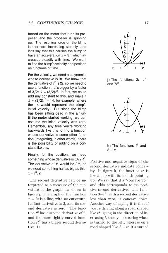
The second derivative can be in-terpreted as a measure of the cur-vature of the graph, as shown infigure j. The graph of the functionx = 2t is a line, with no curvature.Its first derivative is 2, and its sec-ond derivative is zero. The func-tion t2 has a second derivative of 2,and the more tightly curved func-tion 7t2 has a bigger second deriva-tive, 14.
j / The functions 2t , t2
and 7t2.
k / The functions t2 and3− t2.
Positive and negative signs of thesecond derivative indicate concav-ity. In figure k, the function t2 islike a cup with its mouth pointingup. We say that it’s “concave up,”and this corresponds to its posi-tive second derivative. The func-tion 3−t2, with a second derivativeless than zero, is concave down.Another way of saying it is that ifyou’re driving along a road shapedlike t2, going in the direction of in-creasing t, then your steering wheelis turned to the left, whereas on aroad shaped like 3 − t2 it’s turned
18 CHAPTER 1. RATES OF CHANGE
to the right.
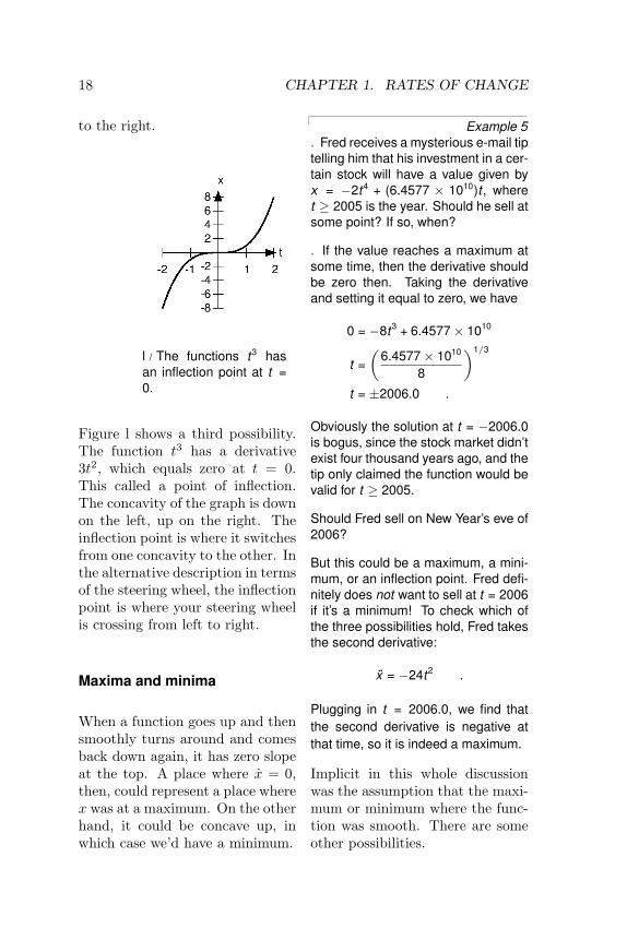
l / The functions t3 hasan inflection point at t =0.
Figure l shows a third possibility.The function t3 has a derivative3t2, which equals zero at t = 0.This called a point of inflection.The concavity of the graph is downon the left, up on the right. Theinflection point is where it switchesfrom one concavity to the other. Inthe alternative description in termsof the steering wheel, the inflectionpoint is where your steering wheelis crossing from left to right.
Maxima and minima
When a function goes up and thensmoothly turns around and comesback down again, it has zero slopeat the top. A place where x = 0,then, could represent a place wherex was at a maximum. On the otherhand, it could be concave up, inwhich case we’d have a minimum.
Example 5. Fred receives a mysterious e-mail tiptelling him that his investment in a cer-tain stock will have a value given byx = −2t4 + (6.4577 × 10¹⁰)t , wheret ≥ 2005 is the year. Should he sell atsome point? If so, when?
. If the value reaches a maximum atsome time, then the derivative shouldbe zero then. Taking the derivativeand setting it equal to zero, we have
0 = −8t3 + 6.4577× 10¹⁰
t =„
6.4577× 10¹⁰
8
«1/3
t = ±2006.0 .
Obviously the solution at t = −2006.0is bogus, since the stock market didn’texist four thousand years ago, and thetip only claimed the function would bevalid for t ≥ 2005.
Should Fred sell on New Year’s eve of2006?
But this could be a maximum, a mini-mum, or an inflection point. Fred defi-nitely does not want to sell at t = 2006if it’s a minimum! To check which ofthe three possibilities hold, Fred takesthe second derivative:
x = −24t2 .
Plugging in t = 2006.0, we find thatthe second derivative is negative atthat time, so it is indeed a maximum.
Implicit in this whole discussionwas the assumption that the maxi-mum or minimum where the func-tion was smooth. There are someother possibilities.

1.2. CONTINUOUS CHANGE 19
In figure m, the function’s mini-mum occurs at an end-point of itsdomain.
m / The function x =√
thas a minimum at t =0, which is not a placewhere x = 0. This point isthe edge of the function’sdomain.
n / The function x = |t |has a minimum at t =0, which is not a placewhere x = 0. This is apoint where the functionisn’t differentiable.
Another possibility is that thefunction can have a minimum ormaximum at some point whereits derivative isn’t well defined.Figure n shows such a situation.
There is a kink in the function att = 0, so a wide variety of linescould be placed through the graphthere, all with different slopes andall staying on one side of the graph.There is no uniquely defined tan-gent line, so the derivative is unde-fined.
Example 6. Rancher Rick has a length of cy-clone fence L with which to enclose arectangular pasture. Show that he canenclose the greatest possible area byforming a square with sides of lengthL/4.
. If the width and length of the rect-angle are t and u, and Rick is go-ing to use up all his fencing material,then the perimeter of the rectangle,2t + 2u, equals L, so for a given width,t , the length is u = L/2 − t . The areais a = tu = t(L/2 − t). The func-tion only means anything realistic for0 ≤ t ≤ L/2, since for values of t out-side this region either the width or theheight of the rectangle would be neg-ative. The function a(t) could there-fore have a maximum either at a placewhere a = 0, or at the endpoints of thefunction’s domain. We can eliminatethe latter possibility, because the areais zero at the endpoints.
To evaluate the derivative, we firstneed to reexpress a as a polynomial:
a = −t2 +L2
t .
The derivative is
a = −2t +L2
.
Setting this equal to zero, we find t =L/4, as claimed. This is a maximum,not a minimum or an inflection point,
20 CHAPTER 1. RATES OF CHANGE
because the second derivative is theconstant a = −2, which is negative forall t , including t = L/4.
PROBLEMS 21
Problems1 Graph the function t2 in theneighborhood of t = 3, draw a tan-gent line, and use its slope to verifythat the derivative equals 2t at thispoint. . Solution, p. 116
2 Graph the function sin et inthe neighborhood of t = 0, draw atangent line, and use its slope toestimate the derivative. Answer:0.5403023058. (You will of coursenot get an answer this precise usingthis technique.)
. Solution, p. 116
3 Differentiate the follow-ing functions with respect to t:1, 7, t, 7t, t2, 7t2, t3, 7t3.
. Solution, p. 117
4 Differentiate 3t7−4t2 +6 withrespect to t. . Solution, p. 117
5 Differentiate at2 + bt+ c withrespect to t.. Solution, p. 117 [Thompson, 1919]
6 Find two different functionswhose derivatives are the constant3, and give a geometrical interpre-tation. . Solution, p. 117
7 Find a function x whosederivative is x = t7. In otherwords, integrate the given func-tion. . Solution, p. 117
8 Find a function x whosederivative is x = 3t7. In otherwords, integrate the given func-tion. . Solution, p. 117
9 Find a function x whosederivative is x = 3t7 − 4t2 + 6.
In other words, integrate the givenfunction. . Solution, p. 118
10 Let t be the time that haselapsed since the Big Bang. In thattime, light, traveling at speed c,has been able to travel a maximumdistance ct. The portion of the uni-verse that we can observe is there-fore a sphere of radius ct, with vol-ume v = (4/3)πr3 = (4/3)π(ct)3.Compute the rate v at which theobservable universe is expanding,and check that your answer has theright units, as in example 2 on page15. . Solution, p. 118
11 Kinetic energy is a measureof an object’s quantity of motion;when you buy gasoline, the energyyou’re paying for will be convertedinto the car’s kinetic energy (actu-ally only some of it, since the en-gine isn’t perfectly efficient). Thekinetic energy of an object withmass m and velocity v is given byK = (1/2)mv2. For a car acceler-ating at a steady rate, with v = at,find the rate K at which the en-gine is required to put out kineticenergy. K, with units of energyover time, is known as the power.Check that your answer has theright units, as in example 2 on page15. . Solution, p. 118
12 A metal square expandsand contracts with temperature,the lengths of its sides varying ac-cording to the equation ` = (1 +αT )`o. Find the rate of changeof its surface area with respect totemperature. That is, find ˙, where

22 CHAPTER 1. RATES OF CHANGE
the variable with respect to whichyou’re differentiating is the tem-perature, T . Check that your an-swer has the right units, as in ex-ample 2 on page 15.
. Solution, p. 118
13 Find the second derivative of2t3 − t. . Solution, p. 119
14 Locate any points of inflec-tion of the function t3 + t2. Verifyby graphing that the concavity ofthe function reverses itself at thispoint. . Solution, p. 119
15 Let’s see if the rule that thederivative of tk is ktk−1 also worksfor k < 0. Use a graph to test oneparticular case, choosing one par-ticular negative value of k, and oneparticular value of t. If it works,what does that tell you about therule? If it doesn’t work?
. Solution, p. 119
16 Two atoms will interact viaelectrical forces between their pro-tons and electrons. To put themat a distance r from one another(measured from nucleus to nu-cleus), a certain amount of energyE is required, and the minimumenergy occurs when the atoms arein equilibrium, forming a molecule.Often a fairly good approximationto the energy is the Lennard-Jonesexpression
E(r) = k
[(ar
)12
− 2(ar
)6]
,
where k and a are constants. Notethat, as proved in chapter 2, therule that the derivative of tk is
ktk−1 also works for k < 0. Showthat there is an equilibrium at r =a. Verify (either by graphing or bytesting the second derivative) thatthis is a minimum, not a maximumor a point of inflection.
. Solution, p. 121
17 Prove that the total numberof maxima and minima possessedby a third-order polynomial is atmost two. . Solution, p. 122

2 To infinity — andbeyond!
a / Gottfried Leibniz(1646-1716)
Little kids readily pick up the ideaof infinity. “When I grow up,I’m gonna have a million Barbies.”“Oh yeah? Well, I’m gonna havea billion.” “Well, I’m gonna haveinfinity Barbies.” “So what? I’llhave two infinity of them.” Adultslaugh, convinced that infinity, ∞,is the biggest number, so 2∞ can’tbe any bigger. This is the ideabehind the joke in the movie ToyStory. Buzz Lightyear’s slogan is“To infinity — and beyond!” Weassume there isn’t any beyond. In-finity is supposed to be the biggestthere is, so by definition there can’tbe anything bigger, right?
2.1 InfinitesimalsActually mathematicians have in-vented several many different log-
ical systems for working with in-finity, and in most of them in-finity does come in different sizesand flavors. Newton, as well asthe German mathematician Leib-niz who invented calculus inde-pendently,1 had a strong intuitiveidea that calculus was really aboutnumbers that were infinitely small:infinitesimals, the opposite of in-finities. For instance, consider thenumber 1.12 = 1.21. That 2 in thefirst decimal place is the same 2that appears in the expression 2tfor the derivative of t2.
b / A close-up view of thefunction x = t2, show-ing the line that con-nects the points (1, 1)and (1.1, 1.21).
1There is some dispute over this point.Newton and his supporters claimed thatLeibniz plagiarized Newton’s ideas, andmerely invented a new notation for them.
23

24 CHAPTER 2. TO INFINITY — AND BEYOND!
Figure b shows the idea visually.The line connecting the points(1, 1) and (1.1, 1.21) is almost in-distinguishable from the tangentline on this scale. Its slope is(1.21 − 1)/(1.1 − 1) = 2.1, whichis very close to the tangent line’sslope of 2. It was a good approx-imation because the points wereclose together, separated by only0.1 on the t axis.
If we needed a better approxi-mation, we could try calculating1.012 = 1.0201. The slope of theline connecting the points (1, 1)and (1.01, 1.0201) is 2.01, which iseven closer to the slope of the tan-gent line.
Another method of visualizing theidea is that we can interpret x = t2
as the area of a square with sidesof length t, as suggested in fig-ure c. We increase t by an in-finitesimally small number dt. Thed is Leibniz’s notation for a verysmall difference, and dt is to beread is a single symbol, “dee-tee,”not as a number d multiplied by
c / A geometrical inter-pretation of the derivativeof t2.
a number t. The idea is that dtis smaller than any ordinary num-ber you could imagine, but it’s notzero. The area of the square is in-creased by dx = 2tdt + dt2, whichis analogous to the finite numbers0.21 and 0.0201 we calculated ear-lier. Where before we divided bya finite change in t such as 0.1 or0.01, now we divide by dt, produc-ing
dxdt
=2t dt+ dt2
dt= 2t+ dt
for the derivative. On a graph likefigure b, dx/dt is the slope of thetangent line: the change in x di-vided by the changed in t.
But adding an infinitesimal num-ber dt onto 2t doesn’t really changeit by any amount that’s even the-oretically measurable in the realworld, so the answer is really 2t.Evaluating it at t = 1 gives theexact result, 2, that the earlierapproximate results, 2.1 and 2.01,were getting closer and closer to.
Example 7To show the power of infinitesimals
and the Leibniz notation, let’s provethat the derivative of t3 is 3t2:
dxdt
=(t + dt)3 − t3
dt
=3t2 dt + 3t dt + dt3
dt= 3t2 + . . . ,
where the dots indicate infinitesimalterms that we can neglect.

2.1. INFINITESIMALS 25
This result required significantsweat and ingenuity when provedon page 107 by the methods ofchapter 1, and not only thatbut the old method would haverequired a completely differentmethod of proof for a function thatwasn’t a polynomial, whereas thenew one can be applied more gen-erally, as shown in the following ex-ample.
Example 8The derivative of x = sin t , with t in
units of radians, is
dxdt
=sin(t + dt)− sin t
dt,
and with the trig identity sin(α + β) =sin α cos β+ cos α sin β, this becomes
=sin t cos dt + cos t sin dt − sin t
dt.
Applying the small-angle approxima-tions sin u ≈ u and cos u ≈ 1, wehave
dxdt
=cos t dt
dt= cos t .
But are the approximations goodenough? The situation is similar to theone we encountered earlier, in whichwe computed (t + dt)2, and neglectedthe dt2 term represented by the smallsquare in figure c. Being a little lesscavalier, I should demonstrate explic-itly that the error introduced by thesmall-angle approximations is really ofthe same order of magnitude as dt2,i.e., a number that is infinitesimallysmall compared even to the infinites-imal size of dt ; I’ve done this on page108. There’s even a second subtle is-sue that I’ve swept under the rug, andI’ll come back to that on page 30.
Figure d shows the graphs of the func-tion and its derivative. Note how thetwo graphs correspond. At t = 0,the slope of sin t is at its largest, andis positive; this is where the deriva-tive, cos t , attains its maximum posi-tive value of 1. At t = π/2, sin t hasreached a maximum, and has a slopeof zero; cos t is zero here. At t = π,in the middle of the graph, sin t has itsmaximum negative slope, and cos t isat its most negative extreme of −1.
Physically, sin t could represent theposition of a pendulum as it movedback and forth from left to right, andcos t would then be the pendulum’svelocity.
d / Graphs of sin t , andits derivative cos t .
Example 9What about the derivative of the co-
sine? The cosine and the sine are re-ally the same function, shifted to theleft or right by π/4. If the derivativeof the sine is the same as itself, butshifted to the left by π/4, then thederivative of the cosine must be a co-sine shifted to the left by π/4:
d cos tdt
= cos(t + π/4)
= − sin t .

26 CHAPTER 2. TO INFINITY — AND BEYOND!
e / Bishop GeorgeBerkeley (1685-1753)
2.2 Safe use ofinfinitesimals
The idea of infinitesimally smallnumbers has always irked purists.One prominent critic of the cal-culus was Newton’s contemporaryGeorge Berkeley, the Bishop ofCloyne. Although some of hiscomplaints are clearly wrong (hedenied the possibility of the sec-ond derivative), there was clearlysomething to his criticism of theinfinitesimals. He wrote sarcas-tically, “They are neither finitequantities, nor quantities infinitelysmall, nor yet nothing. May we notcall them ghosts of departed quan-tities?”
Infinitesimals seemed scary, be-cause if you mishandled them, youcould prove absurd things. Forexample, let du be an infinitesi-mal. Then 2du is also infinites-imal. Therefore both 1/du and1/(2du) equal infinity, so 1/du =1/(2du). Multiplying by du onboth sides, we have a proof that1 = 1/2.
In the eighteenth century, the useof infinitesimals became like adul-tery: commonly practiced, butshameful to admit to in polite cir-cles. Those who used them learnedcertain rules of thumb for handlingthem correctly. For instance, theywould identify the flaw in my proofof 1 = 1/2 as my assumption thatthere was only one size of infinity,when actually 1/du should be in-terpreted as an infinity twice as bigas 1/(2du). The use of the sym-bol ∞ played into this trap, be-cause the use of a single symbolfor infinity implied that infinitiesonly came in one size. However,the practitioners of infinitesimalshad trouble articulating a clearset of principles for their properuse, and couldn’t prove that a self-consistent system could be builtaround them.
By the twentieth century, whenI learned calculus, a clear con-sensus had formed that infiniteand infinitesimal numbers weren’tnumbers at all. A notation likedx/dt, my calculus teacher toldme, wasn’t really one number di-vided by another, it was merely asymbol for the limit
lim∆t→0
∆x∆t
,
where ∆x and ∆t represented fi-nite changes. I’ll give a formal def-inition (actually two different for-mal definitions) of the term “limit”in section 2.9, but intuitively theconcept is that is that we can goodan approximation to the derivative

2.2. SAFE USE OF INFINITESIMALS 27
as we like, provided that we make∆t small enough.
That satisfied me until we got toa certain topic (implicit differen-tiation) in which we were encour-aged to break the dx away fromthe dt, leaving them on oppositesides of the equation. I button-holed my teacher after class andasked why he was now doing whathe’d told me you couldn’t reallydo, and his response was that dxand dt weren’t really numbers, butmost of the time you could getaway with treating them as if theywere, and you would get the rightanswer in the end. Most of thetime!? That bothered me. Howwas I supposed to know when itwasn’t “most of the time?”
f / Abraham Robinson(1918-1974)
But unknown to me and myteacher, mathematician AbrahamRobinson had already shown in the1960’s that it was possible to con-struct a self-consistent number sys-
tem that included infinite and in-finitesimal numbers. He called itthe hyperreal number system, andit included the real numbers as asubset.2
Moreover, the rules for what youcan and can’t do with the hy-perreals turn out to be extremelysimple. Take any true statementabout the real numbers. Supposeit’s possible to translate it into astatement about the hyperreals inthe most obvious way, simply byreplacing the word “real” with theword “hyperreal.” Then the trans-lated statement is also true. Thisis known as the transfer principle.
Let’s look back at my bogus proofof 1 = 1/2 in light of this sim-ple principle. The final step ofthe proof, for example, is perfectlyvalid: multiplying both sides of theequation by the same thing. Thefollowing statement about the realnumbers is true:
For any real numbers a, b, andc, if a = b, then ac = bc.
2The reader who wants tolearn more about the hyperrealsystem might want to start byreading K. Stroyan’s articles athttp://www.math.uiowa.edu/~stroyan/
InfsmlCalculus/InfsmlCalc.htm. Formore depth, one could next read therelevant parts of Keisler’s Elemen-tary Calculus: An Approach UsingInfinitesimals, an out-of-print calculustext that uses infinitesimals, availablefor free from the author’s web site athttp://www.math.wisc.edu/~keisler/
calc.html. The standard (difficult)treatise on the subject is Robinson’sNon-Standard Analysis.

28 CHAPTER 2. TO INFINITY — AND BEYOND!
This can be translated in an obvi-ous way into a statement about thehyperreals:
For any hyperreal numbers a,b, and c, if a = b, then ac = bc.
However, what about the state-ment that both 1/du and 1/(2du)equal infinity, so they’re equal toeach other? This isn’t the trans-lation of a statement that’s trueabout the reals, so there’s no rea-son to believe it’s true — and infact it’s false.
What the transfer principle tells usis that the real numbers as we nor-mally think of them are not uniquein obeying the ordinary rules of al-gebra. There are completely dif-ferent systems of numbers, suchas the hyperreals, that also obeythem.
How, then, are the hyperreals evendifferent from the reals, if every-thing that’s true of one is true ofthe other? But recall that thetransfer principle doesn’t guaran-tee that every statement about thereals is also true of the hyperre-als. It only works if the statementabout the reals can be translatedinto a statement about the hyper-reals in the most simple, straight-forward way imaginable, simply byreplacing the word “real” with theword “hyperreal.” Here’s an ex-ample of a true statement aboutthe reals that can’t be translatedin this way:
For any real number a, there
is an integer n that is greaterthan a.
This one can’t be translated sosimplemindedly, because it refersto a subset of the reals calledthe integers. It might be possi-ble to translate it somehow, butit would require some insight intothe correct way to translate thatword “integer.” The transfer prin-ciple doesn’t apply to this state-ment, which indeed is false for thehyperreals, because the hyperre-als contain infinite numbers thatare greater than all the integers.In fact, the contradiction of thisstatement can be taken as a def-inition of what makes the hyper-reals special, and different fromthe reals: we assume that there isat least one hyperreal number, H,which is greater than all the inte-gers.
As an analogy from everyday life,consider the following statementsabout the student body of the highschool I attended:
1. Every student at my highschool had two eyes and a face.2. Every student at my highschool who was on the footballteam was a jerk.
Let’s try to translate these intostatements about the populationof California in general. The stu-dent body of my high school is likethe set of real numbers, and thepresent-day population of Califor-nia is like the hyperreals. State-ment 1 can be translated mind-

2.2. SAFE USE OF INFINITESIMALS 29
lessly into a statement that ev-ery Californian has two eyes anda face; we simply substitute “ev-ery Californian” for “every studentat my high school.” But state-ment 2 isn’t so easy, because itrefers to the subset of studentswho were on the football team,and it’s not obvious what the cor-responding subset of Californianswould be. Would it include ev-erybody who played high school,college, or pro football? Maybeit shouldn’t include the pros, be-cause they belong to an organiza-tion covering a region bigger thanCalifornia. Statement 2 is the kindof statement that the transfer prin-ciple doesn’t apply to.3
Example 10As a nontrivial example of how to ap-
ply the transfer principle, let’s considerhow to handle expressions like theone that occurred when we wanted todifferentiate t2 using infinitesimals:
d`t2´
dt= 2t + dt .
I argued earlier than 2t +dt is so closeto 2t that for all practical purposes, theanswer is really 2t . But is it really validin general to say that 2t + dt is thesame hyperreal number as 2t? No.
3For a slightly more precise and for-mal statement of the transfer principle,the idea being expressed here is that thephrases “for any” and “there exists” canonly be used in phrases like “for any realnumber x” and “there exists a real num-ber y such that. . . ” The transfer prin-ciple does not apply to statements like“there exists an integer x such that. . . ”or even “there exists a subset of the realnumbers such that. . . ”
We can apply the transfer principle tothe following statement about the re-als:
For any real numbers a and b,with b 6= 0, a + b 6= a.
Since dt isn’t zero, 2t + dt 6= 2t .
More generally, example 10 leadsus to visualize every number as be-ing surrounded by a “halo” of num-bers that don’t equal it, but dif-fer from it by only an infinitesi-mal amount. Just as a magnify-ing glass would allow you to seethe fleas on a dog, you would needan infinitely strong microscope tosee this halo. This is similar tothe idea that every integer is sur-rounded by a bunch of fractionsthat would round off to that inte-ger. We can define the standardpart of a finite hyperreal number,which means the unique real num-ber that differs from it infinitesi-mally. For instance, the standardpart of 2t+ dt, notated st(2t+ dt),equals 2t. The derivative of a func-tion should actually be defined asthe standard part of dx/dt, butwe often write dx/dt to mean thederivative, and don’t worry aboutthe distinction.
One of the things Bishop Berkeleydisliked about infinitesimals wasthe idea that they existed in akind of hierarchy, with dt2 beingnot just infinitesimally small, butinfinitesimally small compared tothe infinitesimal dt. If dt is theflea on a dog, then dt2 is a sub-microscopic flea that lives on the

30 CHAPTER 2. TO INFINITY — AND BEYOND!
flea, as in Swift’s doggerel: “Bigfleas have little fleas/ On theirbacks to ride ’em,/ and little fleashave lesser fleas,/And so, ad in-finitum.” Berkeley’s criticism wasoff the mark here: there is such ahierarchy. Our basic assumptionabout the hyperreals was that theycontain at least one infinite num-ber, H, which is bigger than allthe integers. If this is true, then1/H must be less than 1/2, lessthan 1/100, less then 1/1, 000, 000— less than 1/n for any integer n.Therefore the hyperreals are guar-anteed to include infinitesimals aswell, and so we have at least threelevels to the hierarchy: infinitiescomparable to H, finite numbers,and infinitesimals comparable to1/H. If you can swallow that,then it’s not too much of a leap toadd more rungs to the ladder, likeextra-small infinitesimals that arecomparable to 1/H2. If this seemsa little crazy, it may comfort youto think of statements about thehyperreals as descriptions of limit-ing processes involving real num-bers. For instance, in the sequenceof numbers 1.12 = 1.21, 1.012 =1.0201, 1.0012 = 1.002001, . . . , it’sclear that the number representedby the digit 1 in the final decimalplace is getting smaller faster thanthe contribution due to the digit 2in the middle.
One subtle issue here, which I al-luded to in the differentiation ofthe sine function on page 25, iswhether the transfer principle is
sufficient to let us define all thefunctions that appear as familiarkeys on a calculator: x2,
√x, sinx,
cosx, ex, and so on. After all,these functions were originally de-fined as rules that would take areal number as an input and give areal number as an output. It’s nottrivially obvious that their defini-tions can naturally be extended totake a hyperreal number as an in-put and give back a hyperreal asan output. Essentially the answeris that we can apply the transferprinciple to them just as we wouldto statements about simple arith-metic, but I’ve discussed this a lit-tle more on page 109.
2.3 The product rule
When I first learned calculus, itseemed to me that if the deriva-tive of 3t was 3, and the deriva-tive of 7t was 7, then the deriva-tive of t multiplied by t ought tobe just plain old t, not 2t. Thereason there’s a factor of 2 in thecorrect answer is that t2 has tworeasons to grow as t gets bigger: itgrows because the first factor of tis increasing, but also because thesecond one is. In general, it’s pos-sible to find the derivative of theproduct of two functions any timewe know the derivatives of the in-dividual functions.
The product ruleIf x and y are both functions of t,then the derivative of their product
2.3. THE PRODUCT RULE 31
is
d(xy)dt
=dxdt· y + x · dy
dt.
The proof is easy. Changing t byan infinitesimal amount dt changesthe product xy by an amount
(x+ dx)(y + dy)− xy= ydx+ xdy + dxdy ,
and dividing by dt makes this into
dxdt· y + x · dy
dt+
dxdydt
,
whose standard part is the resultto be proved.
Example 11. Find the derivative of the functiont sin t .
.
d(t sin t)dt
= t · d(sin t)dt
+dtdt· sin t
= t cos t + sin t
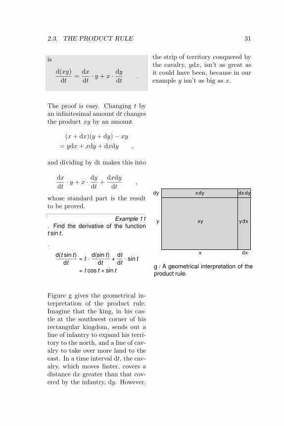
Figure g gives the geometrical in-terpretation of the product rule.Imagine that the king, in his cas-tle at the southwest corner of hisrectangular kingdom, sends out aline of infantry to expand his terri-tory to the north, and a line of cav-alry to take over more land to theeast. In a time interval dt, the cav-alry, which moves faster, covers adistance dx greater than that cov-ered by the infantry, dy. However,
the strip of territory conquered bythe cavalry, ydx, isn’t as great asit could have been, because in ourexample y isn’t as big as x.
g / A geometrical interpretation of theproduct rule.

32 CHAPTER 2. TO INFINITY — AND BEYOND!
A helpful feature of the Leibniznotation is that one can easilyuse it to check whether the unitsof an answer make sense. If wemeasure distances in meters andtime in seconds, then xy has unitsof square meters (area), and sodoes the change in the area, d(xy).Dividing by dt gives the numberof square meters per second be-ing conquered. On the right-handside of the product rule, dx/dthas units of meters per second(velocity), and multiplying it byy makes the units square metersper second, which is consistentwith the left-hand side. The unitsof the second term on the rightlikewise check out. Some begin-ners might be tempted to guessthat the product rule would bed(xy)/dt = (dx/dt)(dy/dt), butthe Leibniz notation instantly re-veals that this can’t be the case,because then the units on the left,m2/s, wouldn’t match the ones onthe right, m2/s2.
Because this unit-checking featureis so helpful, there is a special wayof writing a second derivative inthe Leibniz notation. What New-ton called x, Leibniz wrote as
d2x
dt2.
Although the different placementof the 2’s on top and bottom seemsstrange and inconsistent to manybeginners, it actually works outnicely. If x is a distance, mea-sured in meters, and t is a time,in units of seconds, then the sec-ond derivative is supposed to haveunits of acceleration, in units ofmeters per second per second, alsowritten (m/s)/s, or m/s2. (Theacceleration of falling objects onEarth is 9.8 m/s2 in these units.)The Leibniz notation is meant tosuggest exactly this: the top of thefraction looks like it has units ofmeters, because we’re not squaringx, while the bottom of the fractionlooks like it has units of seconds,because it looks like we’re squar-ing dt. Therefore the units comeout right. It’s important to realize,however, that the symbol d isn’t anumber (not a real one, and not ahyperreal one, either), so we can’treally square it; the notation is notto be taken as a literal statementabout infinitesimals.

2.4. THE CHAIN RULE 33
Example 12A tricky use of the product rule is to
find the derivative of√
t . Since√
t canbe written as t1/2, we might suspectthat the rule d(tk )/dt = ktk−1 wouldwork, giving a derivative 1
2 t−1/2 =1/(2√
t). However, the methods usedto prove that rule in chapter 1 onlywork if k is an integer, so the best wecould do would be to confirm our con-jecture approximately by graphing.
Using the product rule, we can writef (t) = d
√t/dt for our unknown deriva-
tive, and back into the result using theproduct rule:
dtdt
=d(√
t√
t)dt
= f (t)√
t +√
t f (t)
= 2f (t)√
t
But dt/dt = 1, so f (t) = 1/(2√
t) asclaimed.
The trick used in example 12 canalso be used to prove that thepower rule d(xn)/dx = nxn−1 ap-plies to cases where n is an integerless than 0, but I’ll instead provethis on page 36 by a technique thatdoesn’t depend on a trick, and alsoapplies to values of n that aren’tintegers.
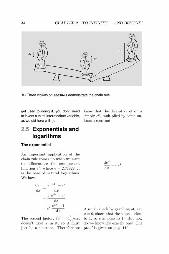
2.4 The chain ruleFigure h shows three clowns on see-saws. If the leftmost clown movesdown by a distance dx, the middleone will come up by dy, but thiswill also cause the one on the rightto move down by dz. If we wantto predict how much the rightmostclown will move in response to acertain amount of motion by theleftmost one, we have
dzdx
=dzdy· dy
dx.
This relation, called the chain rule,allows us to calculate a derivativeof a function defined by one func-tion inside another. The proof,given on page 110, is essentiallyjust the application of the trans-fer principle. (As is often the case,the proof using the hyperreals ismuch simpler than the one usingreal numbers and limits.)
Example 13. Find the derivative of the functionz(x) = sin(x2).
. Let y (x) = x2, so that z(x) =sin(y (x)). Then
dzdx
=dzdy· dy
dx= cos(y ) · 2x
= 2x cos(x2)
The way people usually say it is thatthe chain rule tells you to take thederivative of the outside function, thesine in this case, and then multiplyby the derivative of “the inside stuff,”which here is the square. Once you
34 CHAPTER 2. TO INFINITY — AND BEYOND!
h / Three clowns on seesaws demonstrate the chain rule.
get used to doing it, you don’t needto invent a third, intermediate variable,as we did here with y .
2.5 Exponentials andlogarithms
The exponential
An important application of thechain rule comes up when we wantto differentiate the omnipresentfunction ex, where e = 2.71828 . . .is the base of natural logarithms.We have
dex
dx=ex+dx − ex
dx
=exedx − ex
dx
= exedx − 1
dx
The second factor,(edx − 1
)/dx,
doesn’t have x in it, so it mustjust be a constant. Therefore we
know that the derivative of ex issimply ex, multiplied by some un-known constant,
dex
dx= c ex.
A rough check by graphing at, sayx = 0, shows that the slope is closeto 1, so c is close to 1. But howdo we know it’s exactly one? Theproof is given on page 110.

2.5. EXPONENTIALS AND LOGARITHMS 35
Example 14. The concentration of a foreign sub-
stance in the bloodstream generallyfalls off exponentially with time as c =coe−t/a, where co is the initial concen-tration, and a is a constant. For caf-feine in adults, a is typically about 7hours. An example is shown in figurei. Differentiate the concentration withrespect to time, and interpret the re-sult. Check that the units of the resultmake sense.
. Using the chain rule,
dcdt
= coe−t/a ·„−1
a
«= −co
ae−t/a
This can be interpreted as the rateat which caffeine is being removedfrom the blood and put into the per-son’s urine. It’s negative because theconcentration is decreasing. Accord-ing to the original expression for x ,a substance with a large a will takea long time to reduce its concentra-tion, since t/a won’t be very big un-less we have large t on top to com-pensate for the large a on the bottom.In other words, larger values of a rep-resent substances that the body hasa harder time getting rid of efficiently.The derivative has a on the bottom,and the interpretation of this is that fora drug that is hard to eliminate, therate at which it is removed from theblood is low.
It makes sense that a has units oftime, because the exponential func-tion has to have a unitless argument,so the units of t/a have to cancel out.The units of the result come from thefactor of co/a, and it makes sense that
the units are concentration divided bytime, because the result representsthe rate at which the concentration ischanging.
i / Example 14. A typ-ical graph of the con-centration of caffeine inthe blood, in units of mil-ligrams per liter, as afunction of time, in hours.
Example 15. Find the derivative of the functiony = 10x .
. In general, one of the tricks to do-ing calculus is to rewrite functions informs that you know how to handle.This one can be rewritten as a base-10 logarithm:
y = 10x
ln y = ln`10x´
ln y = x ln 10
y = ex ln 10
Applying the chain rule, we have thederivative of the exponential, which isjust the same exponential, multipliedby the derivative of the inside stuff:
dydx
= ex ln 10 · ln 10 .
36 CHAPTER 2. TO INFINITY — AND BEYOND!
In other words, the “c” referred to inthe discussion of the derivative of ex
becomes c = ln 10 in the case of thebase-10 exponential.
The logarithm
The natural logarithm is the func-tion that undoes the exponential.In a situation like this, we have
dydx
=1
dx/dy,
where on the left we’re thinking ofy as a function of x, and on theright we consider x to be a functionof y. Applying this to the naturallogarithm,
y = lnxx = ey
dxdy
= ey
dydx
=1ey
=1x
d lnxdx
=1x
.
This is noteworthy because itshows that there must be an ex-ception to the rule that the deriva-tive of xn is nxn−1, and the inte-gral of xn−1 is xn/n. (On page33 I remarked that this rule couldbe proved using the product rulefor negative integer values of k,but that I would give a simpler,less tricky, and more general proof
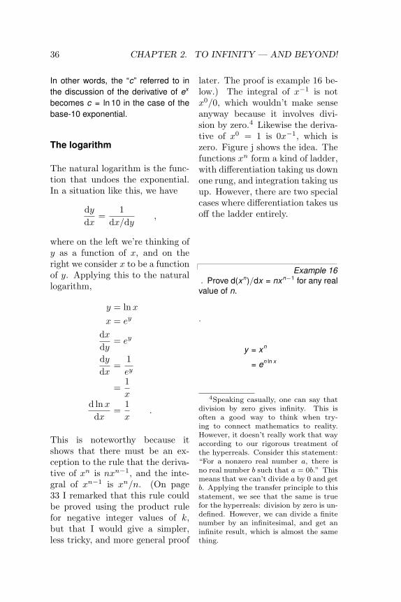
later. The proof is example 16 be-low.) The integral of x−1 is notx0/0, which wouldn’t make senseanyway because it involves divi-sion by zero.4 Likewise the deriva-tive of x0 = 1 is 0x−1, which iszero. Figure j shows the idea. Thefunctions xn form a kind of ladder,with differentiation taking us downone rung, and integration taking usup. However, there are two specialcases where differentiation takes usoff the ladder entirely.
Example 16. Prove d(xn)/dx = nxn−1 for any realvalue of n.
.
y = xn
= en ln x
4Speaking casually, one can say thatdivision by zero gives infinity. This isoften a good way to think when try-ing to connect mathematics to reality.However, it doesn’t really work that wayaccording to our rigorous treatment ofthe hyperreals. Consider this statement:“For a nonzero real number a, there isno real number b such that a = 0b.” Thismeans that we can’t divide a by 0 and getb. Applying the transfer principle to thisstatement, we see that the same is truefor the hyperreals: division by zero is un-defined. However, we can divide a finitenumber by an infinitesimal, and get aninfinite result, which is almost the samething.

2.6. QUOTIENTS 37
j / Differentiation and integration offunctions of the form xn. Constantsout in front of the functions are notshown, so keep in mind that, for ex-ample, the derivative of x2 isn’t x , it’s2x .
By the chain rule,
dydx
= en ln x · nx
= xn · nx
= nxn−1 .
(For n = 0, the result is zero.)
When I started the discussion ofthe derivative of the logarithm, Iwrote y = lnx right off the bat.That meant I was implicitly as-suming x was positive. More gen-erally, the derivative of ln |x| equals1/x, regardless of the sign (seeproblem 24 on page 53).
2.6 QuotientsSo far we’ve been successful witha divide-and-conquer approach todifferentiation: the product ruleand the chain rule offer meth-ods of breaking a function downinto simpler parts, and finding thederivative of the whole thing based
on knowledge of the derivatives ofthe parts. We know how to findthe derivatives of sums, differences,and products, so the obvious nextstep is to look for a way of handlingdivision. This is straightforward,since we know that the derivativeof the function function 1/u = u−1
is −u−2. Let u and v be functionsof x. Then by the product rule,
d(v/u)dx
=dvdx· 1u
+ v · d(1/u)dx
and by the chain rule,
d(v/u)dx
=dvdx· 1u− v · 1
u2
dudx
This is so easy to rederive on de-mand that I suggest not memoriz-ing it.
By the way, notice how the no-tation becomes a little awkwardwhen we want to write a derivativelike d(v/u)/dx. When we’re differ-entiating a complicated function,it can be uncomfortable trying tocram the expression into the top ofthe d . . . /d . . . fraction. Thereforeit would be more common to writesuch an expression like this:
ddx
( vu
)This could be considered an abuseof notation, making d look like anumber being divided by anothernumber dx, when actually d ismeaningless on its own. On theother hand, we can consider thesymbol d/dx to represent the op-eration of differentiation with re-spect to x; such an interpretation

38 CHAPTER 2. TO INFINITY — AND BEYOND!
will seem more natural to thosewho have been inculcated with thetaboo against considering infinites-imals as numbers in the first place.
Using the new notation, the quo-tient rule becomes
ddx
( vu
)=
1u· dv
dx− v
u2· du
dx.
The interpretation of the minussign is that if u increases, v/u de-creases.
Example 17. Differentiate y = x/(1 + 3x), andcheck that the result makes sense.
. We identify v with x and u with 1+x .The result is
ddx
“vu
”=
1u· dv
dx− v
u2 ·dudx
=1
1 + x− 3x
(1 + x)2
One way to check that the resultmakes sense it to consider extremevalues of x . For very large values ofx , the 1 on the bottom of x/(1 + x) be-comes negligible compared to the 3x ,and the function y approaches x/3x =1/3 as a limit. Therefore we expectthat the derivative dy/dx should ap-proach zero, since the derivative ofa constant is zero. It works: plug-ging in bigger and bigger numbers forx in the expression for the derivativedoes give smaller and smaller results.(In the second term, the denominatorgets bigger faster than the numerator,because it has a square in it.)
Another way to check the result is toverify that the units work out. Sup-pose arbitrarily that x has units of gal-lons. (If the 3 on the bottom is unitless,
then the 1 would have to represent 1gallon, since you can’t add things thathave different units.) The function y isdefined by an expression with units ofgallons divided by gallons, so y is unit-less. Therefore the derivative dy/dxshould have units of inverse gallons.Both terms in the expression for thederivative do have those units, so theunits of the answer check out.
2.7 Differentiation ona computer
In this chapter you’ve learned a setof rules for evaluating derivatives:derivatives of products, quotients,functions inside other functions,etc. Because these rules exist,it’s always possible to find aformula for a function’s derivative,given the formula for the originalfunction. Not only that, but thereis no real creativity required, so acomputer can be programmed todo all the drudgery. For example,you can download a free, open-source program called Yacas fromyacas.sourceforge.net andinstall it on a Windows or Linuxmachine. There is even a versionyou can run in a web browser with-out installing any special software:http://yacas.sourceforge.net/yacasconsole.html .A typical session with Yacas lookslike this:
Example 18D(x) x^2
2*x
D(x) Exp(x^2)
2*x*Exp(x^2)
2.7. DIFFERENTIATION ON A COMPUTER 39
D(x) Sin(Cos(Sin(x)))
-Cos(x)*Sin(Sin(x))
*Cos(Cos(Sin(x)))
Upright type represents your in-put, and italicized type is the pro-gram’s output.
First I asked it to differentiate x2
with respect to x, and it told methe result was 2x. Then I didthe derivative of ex
2, which I also
could have done fairly easily byhand. (If you’re trying this outon a computer as you real along,make sure to capitalize functionslike Exp, Sin, and Cos.) FinallyI tried an example where I didn’tknow the answer off the top of myhead, and that would have been alittle tedious to calculate by hand.
Unfortunately things are a littleless rosy in the world of integrals.There are a few rules that can helpyou do integrals, e.g., that the inte-gral of a sum equals the sum of theintegrals, but the rules don’t coverall the possible cases. Using Ya-cas to evaluate the integrals of thesame functions, here’s what hap-pens.5
Example 19Integrate(x) x^2
x^3/3
Integrate(x) Exp(x^2)
Integrate(x)Exp(x^2)
Integrate(x)
Sin(Cos(Sin(x)))
5If you’re trying these on your owncomputer, note that the long input linefor the function sin cos sinx shouldn’t bebroken up into two lines as shown in thelisting.
Integrate(x)
Sin(Cos(Sin(x)))
The first one works fine, and Ican easily verify that the answeris correct, by taking the derivativeof x3/3, which is x2. (The an-swer could have been x3/3 + 7, orx3/3+c, where c was any constant,but Yacas doesn’t bother to tell usthat.) The second and third onesdon’t work, however; Yacas justspits back the input at us withoutmaking any progress on it. Andit may not be because Yacas isn’tsmart enough to figure out theseintegrals. The function ex
2can’t
be integrated at all in terms of aformula containing ordinary oper-ations and functions such as ad-dition, multiplication, exponentia-tion, trig functions, exponentials,and so on.
That’s not to say that a programlike this is useless. For example,here’s an integral that I wouldn’thave known how to do, but thatYacas handles easily:
Example 20Integrate(x) Sin(Ln(x))
(x*Sin(Ln(x)))/2
-(x*Cos(Ln(x)))/2
This one is easy to check by dif-ferentiating, but I could have beenmarooned on a desert island for adecade before I could have figuredit out in the first place. There arevarious rules, then, for integration,but they don’t cover all possiblecases as the rules for differentiationdo, and sometimes it isn’t obviouswhich rule to apply. Yacas’s ability
40 CHAPTER 2. TO INFINITY — AND BEYOND!
to integrate sin lnx shows that ithad a rule in its bag of tricks thatI don’t know, or didn’t remember,or didn’t realize applied to this in-tegral.
Back in the 17th century, whenNewton and Leibniz invented cal-culus, there were no computers, soit was a big deal to be able to finda simple formula for your result.Nowadays, however, it may not besuch a big deal. Suppose I want tofind the derivative of sin cos sinx,evaluated at x = 1. I can do some-thing like this on a calculator:
Example 21sin cos sin 1 =
0.61813407
sin cos sin 1.0001 =
0.61810240
(0.61810240-0.61813407)
/.0001 =
-0.3167
I have the right answer, withplenty of precision for most realis-tic applications, although I mighthave never guessed that the myste-rious number −0.3167 was actually−(cos 1)(sin sin 1)(cos cos sin 1).This could get a little tedious if Iwanted to graph the function, forinstance, but then I could just usea computer spreadsheet, or writea little computer program. In thischapter, I’m going to show youhow to do derivatives and integralsusing simple computer programs,using Yacas. The following littleYacas program does the samething as the set of calculatoroperations shown above:
Example 221 f(x):=Sin(Cos(Sin(x)))
2 x:=1
3 dx:=.0001
4 N( (f(x+dx)-f(x))/dx )
-0.3166671628
(I’ve omitted all of Yacas’s outputexcept for the final result.) Line1 defines the function we want todifferentiate. Lines 2 and 3 givevalues to the variables x and dx.Line 4 computes the derivative; theN( ) surrounding the whole thingis our way of telling Yacas that wewant an approximate numerical re-sult, rather than an exact symbolicone.
An interesting thing to try now isto make dx smaller and smaller,and see if we get better and bet-ter accuracy in our approximationto the derivative.
Example 235 g(x,dx):=
N( (f(x+dx)-f(x))/dx )
6 g(x,.1)
-0.3022356406
7 g(x,.0001)
-0.3166671628
8 g(x,.0000001)
-0.3160458019
9 g(x,.00000000000000001)
0
Line 5 defines the derivative func-tion. It needs to know both x anddx. Line 6 computes the derivativeusing dx = 0.1, which we expect tobe a lousy approximation, since dxis really supposed to be infinitesi-mal, and 0.1 isn’t even that small.Line 7 does it with the same value

2.8. CONTINUITY 41
of dx we used earlier. The two re-sults agree exactly in the first dec-imal place, and approximately inthe second, so we can be prettysure that the derivative is −0.32to two figures of precision. Line8 ups the ante, and produces a re-sult that looks accurate to at least3 decimal places. Line 9 attemptsto produce fantastic precision byusing an extremely small value ofdx. Oops — the result isn’t bet-ter, it’s worse! What’s happenedhere is that Yacas computed f(x)and f(x + dx), but they were thesame to within the precision it wasusing, so f(x+ dx)−f(x) roundedoff to zero.6
Example 23 demonstrates the con-cept of how a derivative can be de-fined in terms of a limit:
dydx
= lim∆x→0
∆y∆x
The idea of the limit is that wecan theoretically make ∆y/∆x ap-proach as close as we like to dy/dx,provided we make ∆x sufficientlysmall. In reality, of course, weeventually run into the limits ofour ability to do the computation,as in the bogus result generated online 9 of the example.
6Yacas can do arithmetic to anyprecision you like, although you mayrun into practical limits due to theamount of memory your computer hasand the speed of its CPU. For fun,try N(Pi,1000), which tells Yacas tocompute π numerically to 1000 decimalplaces.
2.8 ContinuityIntuitively, a continuous functionis one whose graph has no suddenjumps in it; the graph is all a singleconnected piece. Formally, f(x)is defined to be continuous if forany real x and any infinitesimal dx,f(x+ dx)− f(x) is infinitesimal.
Example 24Let the function f be defined by f (x) =0 for x ≤ 0, and f (x) = 1 for x > 0.Then f (x) is discontinuous, since fordx > 0, f (0+dx)− f (0) = 1, which isn’tinfinitesimal.
If a function is discontinuous at agiven point, then it is not differen-tiable at that point. On the otherhand, a function like y = |x| showsthat a function can be continuouswithout being differentiable.
Another way of thinking aboutcontinuous functions is given bythe intermediate value theorem.Intuitively, it says that if you aremoving continuously along a road,and you get from point A to pointB, then you must also visit everyother point along the road; only byteleporting (by moving discontin-uously) could you avoid doing so.More formally, the theorem statesthat if y is a continuous functionon the interval from a to b, andif y takes on values y1 and y2 atcertain points within this interval,then for any y3 between y1 and y2,there is some x in the interval forwhich y(x) = y3.7
7For a proof of the intermediate value

42 CHAPTER 2. TO INFINITY — AND BEYOND!
2.9 LimitsHistorically, the calculus of in-finitesimals as created by New-ton and Leibniz was reinterpretedin the nineteenth century byCauchy, Bolzano, and Weierstrassin terms of limits. All mathemati-cians learned both languages, andswitched back and forth betweenthem effortlessly, like the lady Ioverheard in a Southern Californiasupermarket telling her mother,“Let’s get that one, con los nuts.”Those who had been trained in in-finitesimals might hear a statementusing the language of limits, buttranslate it mentally into infinites-imals; to them, every statementabout limits was really a state-ment about infinitesimals. To theiryounger colleagues, trained usinglimits, every statement about in-finitesimals was really to be under-stood as shorthand for a limitingprocess. When Robinson laid therigorous foundations for the hyper-real number system in the 1960’s, acommon objection was that it wasreally nothing new, because ev-ery statement about infinitesimalswas really just a different way ofexpressing a corresponding state-ment about limits; of course thesame could have been said aboutWeierstrass’s work of the preced-ing century! In reality, all prac-
theorem starting from our definitionof continuity, see Keisler’s Elemen-tary Calculus: An Approach UsingInfinitesimals, p. 162, available online athttp://www.math.wisc.edu/~keisler/
calc.html.
titioners of calculus had realizedall along that different approachesworked better for different prob-lems; problem 11 on page 68 is anexample of a result that is mucheasier to prove with infinitesimalsthan with limits.
The Weierstrass definition of alimit is this:
Definition of the limitWe say that ` is the limit of thefunction f(x) as x approaches a,written
limx→a
f(x) = ` ,
if the following is true: for any realnumber ε, there exists another realnumber δ such that for all x in theinterval a−δ ≤ x ≤ a+δ, the valueof f lies within the range from `−εto `+ ε.
Intuitively, the idea is that if I wantyou to make f(x) close to `, I justhave to tell you how close, and youcan tell me that it will be that closeas long as x is within a certain dis-tance of a.
In terms of infinitesimals, we have:
Definition of the limitWe say that ` is the limit of thefunction f(x) as x approaches a,written
limx→a
f(x) = ` ,
if the following is true: for any in-finitesimal number dx, the value of

2.9. LIMITS 43
f(x+dx) is finite, and the standardpart of f(x+ dx) equals `.
The two definitions are equivalent.
Sometimes a limit can be evaluatedsimply by plugging in numbers:
Example 25. Evaluate
limx→0
11 + x
.
. Plugging in x = 0, we find that thelimit is 1.
In some examples, plugging in failsif we try to do it directly, but canbe made to work if we massage theexpression into a different form:
Example 26. Evaluate
limx→0
2x + 7
1x + 8686
.
. Plugging in x = 0 fails because divi-sion by zero is undefined.
Intuitively, however, we expect that thelimit will be well defined, and will equal2, because for very small values ofx , the numerator is dominated by the2/x term, and the denominator by the1/x term, so the 7 and 8686 terms willmatter less and less as x gets smallerand smaller.
To demonstrate this more rigorously, atrick that works is to multiply both thetop and the bottom by x , giving
2 + 7x1 + 8686x
,
which equals 2 when we plug in x = 0,so we find that the limit is zero.
This example is a little subtle, becausewhen x equals zero, the function is notdefined, and moreover it would not bevalid to multiply both the top and thebottom by x . In general, it’s not validalgebra to multiply both the top andthe bottom of a fraction by 0, becausethe result is 0/0, which is undefined.But we didn’t actually multiply both thetop and the bottom by zero, becausewe never let x equal zero. Both theWeierstrass definition and the defini-tion in terms of infinitesimals only re-fer to the properties of the function in aregion very close to the limiting point,not at the limiting point itself.
This is an example in which the func-tion was not well defined at a certainpoint, and yet the limit of the functionwas well defined as we approachedthat point. In a case like this, wherethere is only one point missing fromthe domain of the function, it is naturalto extend the definition of the functionby filling in the “gap tooth.” Example28 shows that this kind of filling-in pro-cedure is not always possible.
Example 27. Investigate the limiting behavior of
1/x2 as x approaches 0, and 1.
. At x = 1, plugging in works, and wefind that the limit is 1.
At x = 0, plugging in doesn’t work,because division by zero is unde-fined. Applying the definition in termsof infinitesimals to the limit as x ap-proaches 0, we need to find out
44 CHAPTER 2. TO INFINITY — AND BEYOND!
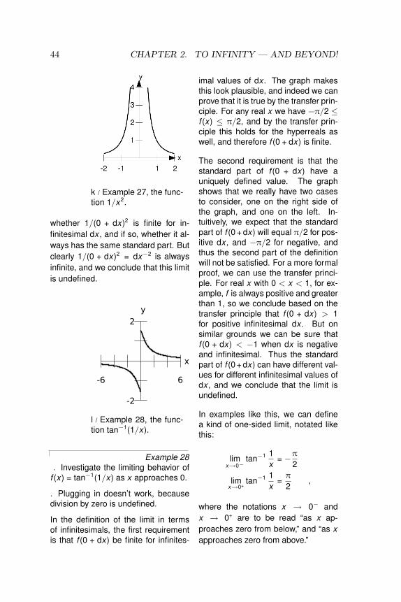
k / Example 27, the func-tion 1/x2.
whether 1/(0 + dx)2 is finite for in-finitesimal dx , and if so, whether it al-ways has the same standard part. Butclearly 1/(0 + dx)2 = dx−2 is alwaysinfinite, and we conclude that this limitis undefined.
l / Example 28, the func-tion tan−1(1/x).
Example 28. Investigate the limiting behavior of
f (x) = tan−1(1/x) as x approaches 0.
. Plugging in doesn’t work, becausedivision by zero is undefined.
In the definition of the limit in termsof infinitesimals, the first requirementis that f (0 + dx) be finite for infinites-
imal values of dx . The graph makesthis look plausible, and indeed we canprove that it is true by the transfer prin-ciple. For any real x we have −π/2 ≤f (x) ≤ π/2, and by the transfer prin-ciple this holds for the hyperreals aswell, and therefore f (0 + dx) is finite.
The second requirement is that thestandard part of f (0 + dx) have auniquely defined value. The graphshows that we really have two casesto consider, one on the right side ofthe graph, and one on the left. In-tuitively, we expect that the standardpart of f (0 + dx) will equal π/2 for pos-itive dx , and −π/2 for negative, andthus the second part of the definitionwill not be satisfied. For a more formalproof, we can use the transfer princi-ple. For real x with 0 < x < 1, for ex-ample, f is always positive and greaterthan 1, so we conclude based on thetransfer principle that f (0 + dx) > 1for positive infinitesimal dx . But onsimilar grounds we can be sure thatf (0 + dx) < −1 when dx is negativeand infinitesimal. Thus the standardpart of f (0 + dx) can have different val-ues for different infinitesimal values ofdx , and we conclude that the limit isundefined.
In examples like this, we can definea kind of one-sided limit, notated likethis:
limx→0−
tan−1 1x
= −π
2
limx→0+
tan−1 1x
=π
2,
where the notations x → 0− andx → 0+ are to be read “as x ap-proaches zero from below,” and “as xapproaches zero from above.”

2.9. LIMITS 45
L’Hopital’s rule
Consider the limit
limx→0
sinxx
.
Plugging in doesn’t work, becausewe get 0/0. Division by zero isundefined, both in the real num-ber system and in the hyperreals.A nonzero number divided by asmall number gives a big number; anonzero number divided by a verysmall number gives a very big num-ber; and a nonzero number dividedby an infinitesimal number givesan infinite number. On the otherhand, dividing zero by zero meanslooking for a solution to the equa-tion 0 = 0q, where q is the resultof the division. But any q is asolution of this equation, so evenspeaking casually, it’s not correctto say that 0/0 is infinite; it’s notinfinite, it’s anything we like.
Since plugging in zero didn’t work,let’s try estimating the limit byplugging in a number for x that’ssmall, but not zero. On a calcula-tor,
sin 0.000010.00001
= 0.999999999983333 .
It looks like the limit is 1. We canconfirm our conjecture to higherprecision using Yacas’s ability todo high-precision arithmetic:
N(Sin(10^-20)/10^-20,50)0.99999999999999999
9999999999999999999
99998333333333
It’s looking pretty one-ish. This isthe idea of the Weierstrass defini-tion of a limit: it seems like we canget an answer as close to 1 as welike, if we’re willing to make x asclose to 0 as necessary. The graphhelps to make this plausible.
m / The graph of sin x/x .
The general idea here is that forsmall values of x, the small-angleapproximation sinx ≈ x obtains,and as x gets smaller and smaller,the approximation gets better andbetter, so sinx/x gets closer andcloser to 1.
But we still haven’t proved rigor-ously that the limit is exactly 1.Let’s try using the definition of thelimit in terms of infinitesimals.
limx→0
sinxx
= st[
sin(0 + dx)0 + dx
]= st
[dx+ . . .
dx
],
46 CHAPTER 2. TO INFINITY — AND BEYOND!
where . . . stands for terms of orderdx2. So
limx→0
sinxx
= st[1 +
. . .
dx
],
= 1 .
This is a special case of a the fol-lowing rule for calculating limitsinvolving 0/0:
L’Hopital’s ruleIf u and v are functions withu(a) = 0 and v(a) = 0, the deriva-tives v(a) and v(a) are defined, andthe derivative v(a) 6= 0, then
limx→a
u
v=u(a)v(a)
.
Proof: Since u(a) = 0, and thederivative du/dx is defined at a,u(a+dx) = du is infinitesimal, andlikewise for v. By the definition ofthe limit, the limit is the standardpart of
u
v=
dudv
=du/dxdv/dx
,
where by assumption the numer-ator and denominator are bothdefined (and finite, because thederivative is defined in terms ofthe standard part). The stan-dard part of a quotient like p/qequals the quotient of the stan-dard parts, provided that both pand q are finite (which we’ve estab-lished), and q 6= 0 (which is trueby assumption). But the standardpart of du/dx is the definition of
the derivative u, and likewise fordv/dx, so this establishes the re-sult.
By the way, the housetop accent onthe “o” in L’Hopital means that inOld French it used to be spelledand pronounced “L’Hospital,” butthe “s” later became silent, so theystopped writing it. So yes, it is thesame word as “hospital.”
Example 29. Evaluate
limx→0
ex − 1x
. Taking the derivatives of the top andbottom, we find ex/1, which equals 1when evaluated at x = 0.
Example 30. Evaluate
limx→1
x − 1x2 − 2x + 1
. Plugging in x = 1 fails, because boththe top and the bottom are zero. Tak-ing the derivatives of the top and bot-tom, we find 1/(2x − 2), which blowsup to infinity when x = 1. To symbol-ize the fact that the limit is undefined,and undefine because it blows up toinfinity, we write
limx→1
x − 1x2 − 2x + 1
=∞

2.9. LIMITS 47
In the following example, we haveto use L’Hopital’s rule twice beforewe get an answer.
Example 31. Evaluate
limx→π
1 + cos x(x − π)2
. Applying L’Hopital’s rule gives
− sin x2(x − π)
,
which still produces 0/0 when we plugin x = π. Going again, we get
− cos x2
=12
.
Another perspective onindeterminate forms
An expression like 0/0, calledan indeterminate form, can bethought of in a different way interms of infinitesimals. SupposeI tell you I have two infinitesimalnumbers d and e in my pocket,and I ask you whether d/e is fi-nite, infinite, or infinitesimal. Youcan’t tell, because d and e mightnot be infinitesimals of the sameorder of magnitude. For instance,if e = 37d, then d/e = 1/37 is fi-nite; but if e = d2, then d/e is in-finite; and if d = e2, then d/e isinfinitesimal. Acting this out withnumbers that are small but not in-
finitesimal,
.001
.037=
137
.001.000001
= 1000
.000001.001
= .001 .
On the other hand, suppose I tellyou I have an infinitesimal num-ber d and a finite number x, andI ask you to speculate about d/x.You know for sure that it’s going tobe infinitesimal. Likewise, you canbe sure that x/d is infinite. Thesearen’t indeterminate forms.
We can do something similar withinfinite numbers. If H and K areboth infinite, then H −K is inde-terminate. It could be infinite, forexample, if H was positive infiniteand K = H/2. On the other hand,it could be finite if H = K + 1.Acting this out with big but finitenumbers,
1000− 500 = 5001001− 1000 = 1 .
Example 32. If H is a positive infinite number,is√
H + 1 −√
H − 1 finite, infinite, in-finitesimal, or indeterminate?
. Trying it with a finite, big number, wehave√
1000001−√
999999
= 1.00000000020373× 10⁻³ ,
which is clearly a wannabe infinitesi-mal. More rigorously, we can rewrite

48 CHAPTER 2. TO INFINITY — AND BEYOND!
the expression as√
H(p
1 + 1/H −p1− 1/H). Since the derivative of
the square root function√
x evaluatedat x = 1 is 1/2, we can approximatethis as
√H»1 +
12H
+ . . .−„
1− 12H
+ . . .«–
=√
H»
1H
+ . . .–
=1√H
,
which is clearly infinitesimal.
Limits at infinity
The definition of the limit in termsof infinitesimals extends immedi-ately to limiting processes wherex gets bigger and bigger, ratherthan closer and closer to some fi-nite value. For example, the func-tion 3 + 1/x clearly gets closerand closer to 3 as x gets biggerand bigger. If a is an infinitenumber, then the definition saysthat evaluating this expression ata + dx, where dx is infinitesimal,gives a result whose standard partis 3. It doesn’t matter that ahappens to be infinite, the defini-tion still works. We also note thatin this example, it doesn’t matterwhat infinite number a is; the limitequals 3 for any infinite a. We canwrite this fact as
limx→∞
(3 +
1x
)= 3 ,
where the symbol ∞ is to be in-terpreted as “nyeah nyeah, I don’t
even care what infinite number youput in here, I claim it will workout to 3 no matter what.” Thesymbol ∞ is not to be interpretedas standing for any specific infinitenumber. That would be the typeof fallacy that lay behind the bo-gus proof on page 26 that 1 = 1/2,which assumed that all infinitieshad to be the same size.
A somewhat different example isthe arctangent function. The arc-tangent of 1000 equals approxi-mately 1.5698, and inputting big-ger and bigger numbers gives an-swers that appear to get closerand closer to π/2 ≈ 1.5707. Butthe arctangent of -1000 is approxi-mately −1.5698, i.e., very close to−π/2. From these numerical ob-servations, we conjecture that
limx→a
tan−1 x
equals π/2 for positive infinite a,but −π/2 for negative infinite a.It would not be correct to write
limx→∞
tan−1 x =π
2[wrong] ,
because it does matter what infi-nite number we pick. Instead wewrite
limx→+∞
tan−1 x =π
2
limx→−∞
tan−1 x = −π2
.
Some expressions don’t have thiskind of limit at all. For exam-ple, if you take the sines of bignumbers like a thousand, a million,
2.9. LIMITS 49
etc., on your calculator, the re-sults are essentially random num-bers lying between −1 and 1. Theydon’t settle down to any particularvalue, because the sine function os-cillates back and forth forever. Toprove formally that limx→+∞ sinxis undefined, consider that the sinefunction, defined on the real num-bers, has the property that youcan always change its result by atleast 0.1 if you add either 1.5 or−1.5 to its input. For example,sin(.8) ≈ 0.717, and sin(.8−1.5) ≈−0.644. Applying the transferprinciple to this statement, we findthat the same is true on the hyper-reals. Therefore there cannot beany value ` that differs infinitesi-mally from sin a for all positive in-finite values of a.
Often we’re interested in findingthe limit as x approaches infinityof an expression that is written asan indeterminate form like H/K,where both H and K are infinite.
Example 33. Evaluate the limit
limx→∞
2x + 7x + 8686
.
. Intuitively, if x gets large enough theconstant terms will be negligible, andthe top and bottom will be dominatedby the 2x and x terms, respectively,giving an answer that approaches 2.
One way to verify this is to divide boththe top and the bottom by x , giving
2 + 7x
1 + 8686x
.
If x is infinite, then the standard partof the top is 2, the standard part of thebottom is 1, and the standard part ofthe whole thing is therefore 2.
Another approach is to use L’Hopital’srule. The derivative of the top is 2, andthe derivative of the bottom is 1, so thelimit is 2/1=2.
50 CHAPTER 2. TO INFINITY — AND BEYOND!
Problems1 Carry out a calculation likethe one in example 7 on page 24to show that the derivative of t4
equals 4t3. . Solution, p. 122
2 Example 9 on page 25 gave atricky argument to show that thederivative of cos t is − sin t. Provethe same result using the methodof example 8 instead.
. Solution, p. 122
3 Suppose H is a big number.Experiment on a calculator to fig-ure out whether
√H + 1−
√H − 1
comes out big, normal, or tiny. Trymaking H bigger and bigger, andsee if you observe a trend. Basedon these numerical examples, forma conjecture about what happensto this expression when H is infi-nite. . Solution, p. 123
4 Suppose dx is a small butfinite number. Experiment on acalculator to figure out how
√dx
compares in size to dx. Try mak-ing dx smaller and smaller, andsee if you observe a trend. Basedon these numerical examples, forma conjecture about what happensto this expression when dx is in-finitesimal. . Solution, p. 123
5 To which of the followingstatements can the transfer prin-ciple be applied? If you think itcan’t be applied to a certain state-ment, try to prove that the state-ment is false for the hyperreals,e.g., by giving a counterexample.
(a) For any real numbers x and y,
x+ y = y + x.(b) The sine of any real number isbetween −1 and 1.(c) For any real number x, thereexists another real number y thatis greater than x.(d) For any real numbers x 6= y,there exists another real number zsuch that x < z < y.(e) For any real numbers x 6= y,there exists a rational number zsuch that x < z < y. (A ratio-nal number is one that can be ex-pressed as an integer divided byanother integer.)(f) For any real numbers x, y, andz, (x+ y) + z = x+ (y + z).(g) For any real numbers x and y,either x < y or x = y or x > y.(h) For any real number x, x+1 6=x. . Solution, p. 123
6 If we want to pump air or waterthrough a pipe, common sense tellsus that it will be easier to movea larger quantity more quicklythrough a fatter pipe. Quantita-tively, we can define the resistance,R, which is the ratio of the pressuredifference produced by the pumpto the rate of flow. A fatter pipewill have a lower resistance. Twopipes can be used in parallel, forinstance when you turn on the wa-ter both in the kitchen and in thebathroom, and in this situation,the two pipes let more water flowthan either would have let flowby itself, which tells us that theyact like a single pipe with somelower resistance. The equation fortheir combined resistance is R =

PROBLEMS 51
1/(1/R1 +1/R2). Analyze the casewhere one resistance is finite, andthe other infinite, and give a phys-ical interpretation. Likewise, dis-cuss the case where one is finite,but the other is infinitesimal.
7 Naively, we would imagine thatif a spaceship traveling at u = 3/4of the speed of light was to shoota missile in the forward directionat v = 3/4 of the speed of light(relative to the ship), then the mis-sile would be traveling at u + v =3/2 of the speed of light. How-ever, Einstein’s theory of relativitytells us that this is too good to betrue, because nothing can go fasterthan light. In fact, the relativis-tic equation for combining veloci-ties in this way is not u + v, butrather (u + v)/(1 + uv). In ordi-nary, everyday life, we never travelat speeds anywhere near the speedof light. Show that the nonrela-tivistic result is recovered in thecase where both u and v are in-finitesimal.
8 Differentiate (2x+ 3)100 withrespect to x. . Solution, p. 124
9 Differentiate (x + 1)100(x +2)200 with respect to x.
. Solution, p. 124
10 Differentiate the followingwith respect to x: e7x, ee
x
. (Inthe latter expression, as in all ex-ponentials nested inside exponen-tials, the evaluation proceeds fromthe top down, i.e., e(ex), not (ee)x.)
. Solution, p. 124
11 Differentiate a sin(bx + c)with respect to x.
. Solution, p. 124
12 Find a function whosederivative with respect to x equalsa sin(bx+ c). That is, find an inte-gral of the given function.
. Solution, p. 124
13 The range of a gun, whenelevated to an angle θ, is given by
R =2v2
gsin θ cos θ .
Find the angle that will producethe maximum range.
. Solution, p. 125
14 The hyperbolic cosine func-tion is defined by
coshx =ex + e−x
2.
Find any minima and maxima ofthis function.
. Solution, p. 125
15 In free fall, the accelerationwill not be exactly constant, dueto air resistance. For example, askydiver does not speed up indefi-nitely until opening her chute, butrather approaches a certain maxi-mum velocity at which the upwardforce of air resistance cancels outthe force of gravity. The expres-sion for the distance dropped by ofa free-falling object, with air resis-tance, is8
d = A ln[cosh
(t
√g
A
)],
8Jan Benacka and Igor Stubna, ThePhysics Teacher, 43 (2005) 432.
52 CHAPTER 2. TO INFINITY — AND BEYOND!
where g is the acceleration the ob-ject would have without air resis-tance, the function cosh has beendefined in problem 14, and A is aconstant that depends on the size,shape, and mass of the object, andthe density of the air. (For a sphereof massm and diameter d droppingin air, A = 4.11m/d2. Cf. problem4, p. 83.)(a) Differentiate this expression tofind the velocity. Hint: In order tosimplify the writing, start by defin-ing some other symbol to stand forthe constant
√g/A.
(b) Show that your answer can bereexpressed in terms of the func-tion tanh defined by tanhx = (ex−e−x)/(ex + e−x).(c) Show that your result for thevelocity approaches a constant forlarge values of t.(d) Check that your answers toparts b and c have units of velocity.
. Solution, p. 125
16 Differentiate tan θ with re-spect to θ. . Solution, p. 126
17 Differentiate 3√x with re-
spect to x. . Solution, p. 126
18 Differentiate the followingwith respect to x:(a) y =
√x2 + 1
(b) y =√x2 + a2
(c) y = 1/√a+ x
(d) y = a/√
(a− x2)
. Solution, p. 126 [Thompson, 1919]
19 Differentiate ln(2t+ 1) withrespect to t. . Solution, p. 126
20 If you know the derivative ofsinx, it’s not necessary to use theproduct rule in order to differenti-ate 3 sinx, but show that using theproduct rule gives the right resultanyway. . Solution, p. 127
21 The Γ function (capitalGreek letter gamma) is a contin-uous mathematical function thathas the property Γ(n) = 1 · 2 ·. . . · (n − 1) for n an integer. Γ(x)is also well defined for values of xthat are not integers, e.g., Γ(1/2)happens to be
√π. Use computer
software that is capable of evalu-ating the Γ function to determinenumerically the derivative of Γ(x)with respect to x, at x = 2. (In Ya-cas, the function is called Gamma.)
. Solution, p. 127
22 For a cylinder of fixedsurface area, what proportion oflength to radius will give the max-imum volume?
. Solution, p. 127
23 This problem is a varia-tion on problem 11 on page 21.Einstein found that the equationK = (1/2)mv2 for kinetic energywas only a good approximation forspeeds much less than the speed oflight, c. At speeds comparable tothe speed of light, the correct equa-tion is
K =12mv
2√1− v2/c2
.
(a) As in the earlier, simpler prob-lem, find the power dK/dt foran object accelerating at a steady
PROBLEMS 53
rate, with v = at.(b) Check that your answer has theright units.(c) Verify that the power requiredbecomes infinite in the limit as vapproaches c, the speed of light.This means that no material ob-ject can go as fast as the speed oflight. . Solution, p. 128
24 Prove, as claimed on page37, that the derivative of ln |x|equals 1/x, for both positive andnegative x. . Solution, p. 128
25 Use a trick similar to the oneused in example 12 to prove thatthe power rule d(xk)/dx = kxk−1
applies to cases where k is an inte-ger less than 0.
. Solution, p. 129 ?
26 The plane of Euclidean geom-etry is today often described as theset of all coordinate pairs (x, y),where x and y are real. We couldinstead imagine the plane F thatis defined in the same way, butwith x and y taken from the setof hyperreal numbers. As a thirdalternative, there is the plane Gin which the finite hyperreals areused. In E, Euclid’s parallel postu-late holds: given a line and a pointnot on the line, there exists ex-actly one line passing through thepoint that does not intersect theline. Does the parallel postulatehold in F? In G? Is it valid to as-sociate only E with the plane de-scribed by Euclid’s axioms? ?
27 (a) Prove, using the Weier-strass definition of the limit,
that if limx→a f(x) = F andlimx→a g(x) = G both exist, themlimx→a[f(x) + g(x)] = F +G, i.e.,that the limit of a sum is the sumof the limits. (b) Prove the samething using the definition of thelimit in terms of infinitesimals.
. Solution, p. 120
28 Sketch the graph of the func-tion e−1/x, and evaluate the follow-ing four limits:
limx→0+
e−1/x
limx→0−
e−1/x
limx→+∞
e−1/x
limx→−∞
e−1/x
29 Verify the following limits.
lims→1
s3 − 1s− 1
= 3
limθ→0
1− cos θθ2
=12
limx→∞
5x2 − 2xx
=∞
limn→∞
n(n+ 1)(n+ 2)(n+ 3)
= 1
limx→∞
ax2 + bx+ c
dx2 + ex+ f=a
d
[Granville, 1911]

54 CHAPTER 2. TO INFINITY — AND BEYOND!

3 Integration3.1 Definite and
indefiniteintegrals
Because any formula can be differ-entiated symbolically to find an-other formula, the main motiva-tion for doing derivatives numeri-cally would be if the function tobe differentiated wasn’t known insymbolic form. A typical exam-ple might be a two-person networkcomputer game, in which playerA’s computer needs to figure outplayer B’s velocity based on knowl-edge of how her position changesover time. But in most cases, it’snumerical integration that’s inter-esting, not numerical differentia-tion.
As a warm-up, let’s see how todo a running sum of a discretefunction using Yacas. The follow-ing program computers the sum1+2+. . .+100 discussed to on page9. Now that we’re writing realcomputer programs with Yacas, itwould be a good idea to enter eachprogram into a file before trying torun it. In fact, some of these exam-ples won’t run properly if you juststart up Yacas and type them inone line at a time. If you’re usingAdobe Reader to read this book,you can do Tools>Basic>Select,select the program, copy it into afile, and then edit out the line num-
bers.
Example 341 n := 1;
2 sum := 0;
3 While (n<=100) [
4 sum := sum+n;
5 n := n+1;
6 ];
7 Echo(sum);
The semicolons are to separate oneinstruction from the next, and theybecome necessary now that we’redoing real programming. Line 1of this program defines the vari-able n, which will take on all thevalues from 1 to 100. Line 2 saysthat we haven’t added anything upyet, so our running sum is zero dofar. Line 3 says to keep on re-peating the instructions inside thesquare brackets until n goes past100. Line 4 updates the runningsum, and line 5 updates the valueof n. If you’ve never done any pro-gramming before, a statement liken:=n+1 might seem like nonsense— how can a number equal itselfplus one? But that’s why we usethe := symbol; it says that we’reredefining n, not stating an equa-tion. If n was previously 37, thenafter this statement is executed, nwill be redefined as 38. To run theprogram on a Linux computer, dothis (assuming you saved the pro-gram in a file named sum.yacas):
% yacas -pc sum.yacas
55

56 CHAPTER 3. INTEGRATION
5050
Here the % symbol is the com-puter’s prompt. The result is5,050, as expected. One way ofstating this result is
100∑n=1
n = 5050 .
The capital Greek letter Σ, sigma,is used because it makes the “s”sound, and that’s the first sound inthe word “sum.” The n = 1 belowthe sigma says the sum starts at 1,and the 100 on top says it ends at100. The n is what’s known as adummy variable: it has no mean-ing outside the context of the sum.Figure a shows the graphical inter-pretation of the sum: we’re addingup the areas of a series of rectan-gular strips. (For clarity, the figureonly shows the sum going up to 7,rather than 100.)
a / Graphical interpreta-tion of the sum 1+2+. . .+7.
Now how about an integral? Fig-ure b shows the graphical inter-
pretation of what we’re trying todo: find the area of the shadedtriangle. This is an example weknow how to do symbolically, sowe can do it numerically as well,and check the answers against eachother. Symbolically, the area isgiven by the integral. To inte-grate the function x(t) = t, weknow we need some function witha t2 in it, since we want somethingwhose derivative is t, and differen-tiation reduces the power by one.The derivative of t2 would be 2trather than t, so what we want isx(t) = t2/2. Let’s compute thearea of the triangle that stretchesalong the t axis from 0 to 100:x(100) = 100/2 = 5000.
b / Graphical interpreta-tion of the integral of thefunction x(t) = t .
Figure c shows how to accomplishthe same thing numerically. Webreak up the area into a wholebunch of very skinny rectangles.Ideally, we’d like to make the widthof each rectangle be an infinitesi-mal number dx, so that we’d be
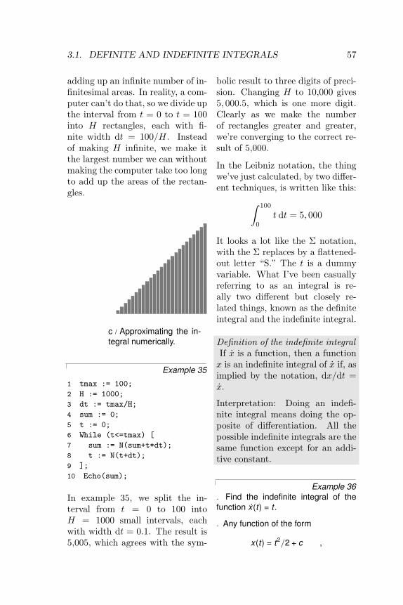
3.1. DEFINITE AND INDEFINITE INTEGRALS 57
adding up an infinite number of in-finitesimal areas. In reality, a com-puter can’t do that, so we divide upthe interval from t = 0 to t = 100into H rectangles, each with fi-nite width dt = 100/H. Insteadof making H infinite, we make itthe largest number we can withoutmaking the computer take too longto add up the areas of the rectan-gles.
c / Approximating the in-tegral numerically.
Example 35
1 tmax := 100;
2 H := 1000;
3 dt := tmax/H;
4 sum := 0;
5 t := 0;
6 While (t<=tmax) [
7 sum := N(sum+t*dt);
8 t := N(t+dt);
9 ];
10 Echo(sum);
In example 35, we split the in-terval from t = 0 to 100 intoH = 1000 small intervals, eachwith width dt = 0.1. The result is5,005, which agrees with the sym-
bolic result to three digits of preci-sion. Changing H to 10,000 gives5, 000.5, which is one more digit.Clearly as we make the numberof rectangles greater and greater,we’re converging to the correct re-sult of 5,000.
In the Leibniz notation, the thingwe’ve just calculated, by two differ-ent techniques, is written like this:∫ 100
0
t dt = 5, 000
It looks a lot like the Σ notation,with the Σ replaces by a flattened-out letter “S.” The t is a dummyvariable. What I’ve been casuallyreferring to as an integral is re-ally two different but closely re-lated things, known as the definiteintegral and the indefinite integral.
Definition of the indefinite integralIf x is a function, then a functionx is an indefinite integral of x if, asimplied by the notation, dx/dt =x.
Interpretation: Doing an indefi-nite integral means doing the op-posite of differentiation. All thepossible indefinite integrals are thesame function except for an addi-tive constant.
Example 36. Find the indefinite integral of thefunction x(t) = t .
. Any function of the form
x(t) = t2/2 + c ,

58 CHAPTER 3. INTEGRATION
where c is a constant, is an indefi-nite integral of this function, since itsderivative is t .
Definition of the definite integralIf x is a function, then the definiteintegral of x from a to b is definedas ∫ b
a
x(t)dt
= limH→∞
H∑i=0
x (a+ i∆t) ,
where ∆t = (b− a)/H.
Interpretation: What we’re calcu-lating is the area under the graphof x, from a to b. (If the graphdips below the t axis, we interpretthe area between it and the axis asa negative area.) The thing insidethe limit is a calculation like theone done in example 35, but gen-eralized to a 6= 0. If H was infinite,then ∆t would be an infinitesimalnumber dt.
3.2 The fundamentaltheorem ofcalculus
The fundamental theorem of calcu-lusLet x be an indefinite integral ofx, and let x be a continuous func-tion (one whose graph is a singleconnected curve). Then
∫ b
a
x(t)dt = x(b)− x(a) .
Interpretation: In the simple ex-amples we’ve been doing so far, wewere able to choose an indefiniteintegral such that x(0) = 0. Inthat case, x(t) is interpreted as thearea from 0 to t, so in the expres-sion x(b) − x(a), we’re taking thearea from 0 to a, but subtractingout the area from 0 to b, whichgives the area from a to b. If wechoose an indefinite integral witha different c, the c’s will just can-cel out anyway in the differencex(b)− x(a).
The fundamental theorem isproved on page 111.
Example 37. Interpret the indefinite integralZ 2
1
1t
dt .
graphically; then evaluate it it bothsymbolically and numerically, andcheck that the two results are consis-tent.
. Figure d shows the graphical inter-pretation. The numerical calculationrequires a trivial variation on the pro-gram from example 35:
a := 1;
b := 2;
H := 1000;
dt := (b-a)/H;

3.3. PROPERTIES OF THE INTEGRAL 59
d / The indefinite integralR 21 (1/t)dt .
sum := 0;
t := a;
While (t<=b) [
sum := N(sum+(1/t)*dt);
t := N(t+dt);
];
Echo(sum);
The result is 0.693897243, andincreasing H to 10,000 gives0.6932221811, so we can befairly confident that the result equals0.693, to 3 decimal places.
Symbolically, the indefinite integral isx = ln t . Using the fundamental the-orem of calculus, the area is ln 2 −ln 1 ≈ 0.693147180559945.
Judging from the graph, it looks plau-sible that the shaded area is about0.7.
This is an interesting example, be-cause the natural log blows up to neg-ative infinity as t approaches 0, so it’snot possible to add a constant ontothe indefinite integral and force it to beequal to 0 at t = 0. Nevertheless, thefundamental theorem of calculus stillworks.
3.3 Properties of theintegral
Let f and g be two functions of x,and let c be a constant. We alreadyknow that for derivatives,
ddx
(f + g) =dfdx
+dgdx
and
ddx
(cf) = cdfdx
.
But since the indefinite integral isjust the operation of undoing aderivative, the same kind of rulesmust hold true for indefinite inte-grals as well:∫
(f + g)dx =∫fdx+
∫gdx
and ∫(cf)dx = c
∫fdx .
And since a definite integral can befound by plugging in the upper andlower limits of integration into theindefinite integral, the same prop-erties must be true of definite inte-grals as well.
Example 38. Evaluate the indefinite integralZ
(x + 2 sin x)dx .
. Using the additive property, the inte-gral becomesZ
xdx +Z
2 sin xdx .
60 CHAPTER 3. INTEGRATION
Then the property of scaling by a con-stant lets us change this toZ
xdx + 2Z
sin xdx .
We need a function whose derivativeis x , which would be x2/2, and onewhose derivative is sin x , which mustbe − cos x , so the result is
12
x2 − 2 cos x + c .
3.4 ApplicationsAverages
In the story of Gauss’s problem ofadding up the numbers from 1 to100, one interpretation of the re-sult, 5,050, is that the average ofall the numbers from 1 to 100 is50.5. This is the ordinary defini-tion of an average: add up all thethings you have, and divide by thenumber of things. (The result inthis example makes sense, becausehalf the numbers are from 1 to 50,and half are from 51 to 100, so theaverage is half-way between 50 and51.)
Similarly, a definite integral canalso be thought of as a kind of aver-age. In general, if y is a function ofx, then the average, or mean, valueof y on the interval from x = a tob can be defined as
y =1
b− a
∫ b
a
y dx .
In the continuous case, dividing byb− a accomplishes the same thing
as dividing by the number of thingsin the discrete case.
Example 39. Show that the definition of the aver-age makes sense in the case wherethe function is a constant.
. If y is a constant, then we can takeit outside of the integral, so
y =1
b − ayZ b
a1 dx
=1
b − ay x |ba
=1
b − ay (b − a)
= y
Example 40. Find the average value of the func-
tion y = x2 for values of x ranging from0 to 1.
y =1
1− 0
Z 1
0x2 dx
=13
x3˛10
=13
The mean value theoremIf the continuous function y(x) hasthe average value y on the inter-val from x = a to b, then y at-tains its average value at least oncein that interval, i.e., there exists ξwith a < ξ < b such that y(ξ) = y.
The mean value theorem is provedon page 112.

3.4. APPLICATIONS 61
Example 41. Verify the mean value theorem fory = x2 on the interval from 0 to 1.
. The mean value is 1/3, as shown inexample 40. This value is achievedat x =
p1/3 = 1/
√3, which lies be-
tween 0 and 1.
Work
In physics, work is a measure ofthe amount of energy transferredby a force; for example, if a horsesets a wagon in motion, the horse’sforce on the wagon is putting someenergy of motion into the wagon.When a force F acts on an ob-ject that moves in the direction ofthe force by an infinitesimal dis-tance dx, the infinitesimal workdone is dW = Fdx. Integratingboth sides, we have W =
∫ baFdx,
where the force may depend on x,and a and b represent the initialand final positions of the object.
Example 42. A spring compressed by an amountx relative to its relaxed length providesa force F = kx . Find the amount ofwork that must be done in order tocompress the spring from x = 0 tox = a. (This is the amount of energystored in the spring, and that energywill later be released into the toy bul-let.)
.
W =Z a
0Fdx
=Z a
0kxdx
=12
kx2˛a0
=12
ka2
The reason W grows like a2, not justlike a, is that as the spring is com-pressed more, more and more effortis required in order to compress it.
Probability
Mathematically, the probabilitythat something will happen can bespecified with a number rangingfrom 0 to 1, with 0 representing im-possibility and 1 representing cer-tainty. If you flip a coin, heads andtails both have probabilities of 1/2.The sum of the probabilities of allthe possible outcomes has to haveprobability 1. This is called nor-malization.
e / Normalization: theprobability of pickingland plus the probabilityof picking water adds upto 1.
So far we’ve discussed random pro-cesses having only two possible

62 CHAPTER 3. INTEGRATION
outcomes: yes or no, win or lose,on or off. More generally, a ran-dom process could have a resultthat is a number. Some processesyield integers, as when you roll adie and get a result from one tosix, but some are not restricted towhole numbers, e.g., the height ofa human being, or the amount oftime that a uranium-238 atom willexist before undergoing radioactivedecay. The key to handling thesecontinuous random variables is theconcept of the area under a curve,i.e., an integral.
f / Probability distribution for the resultof rolling a single die.
Consider a throw of a die. If the dieis “honest,” then we expect all sixvalues to be equally likely. Since allsix probabilities must add up to 1,then probability of any particularvalue coming up must be 1/6. Wecan summarize this in a graph, f.Areas under the curve can be inter-preted as total probabilities. Forinstance, the area under the curvefrom 1 to 3 is 1/6+1/6+1/6 = 1/2,so the probability of getting a re-
sult from 1 to 3 is 1/2. The func-tion shown on the graph is calledthe probability distribution.
g / Rolling two dice and adding themup.
Figure g shows the probabilities ofvarious results obtained by rollingtwo dice and adding them to-gether, as in the game of craps.The probabilities are not all thesame. There is a small probabilityof getting a two, for example, be-cause there is only one way to do it,by rolling a one and then anotherone. The probability of rolling aseven is high because there are sixdifferent ways to do it: 1+6, 2+5,etc.
If the number of possible outcomesis large but finite, for example thenumber of hairs on a dog, thegraph would start to look like asmooth curve rather than a ziggu-rat.
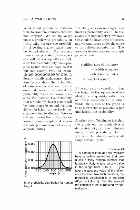
3.4. APPLICATIONS 63
What about probability distribu-tions for random numbers that arenot integers? We can no longermake a graph with probability onthe y axis, because the probabil-ity of getting a given exact num-ber is typically zero. For instance,there is zero probability that a per-son will be exactly 200 cm tall,since there are infinitely many pos-sible results that are close to 200but not exactly two, for exam-ple 199.99999999687687658766. Itdoesn’t usually make sense, there-fore, to talk about the probabilityof a single numerical result, but itdoes make sense to talk about theprobability of a certain range of re-sults. For instance, the probabilitythat a randomly chosen person willbe more than 170 cm and less than200 cm in height is a perfectly rea-sonable thing to discuss. We canstill summarize the probability in-formation on a graph, and we canstill interpret areas under the curveas probabilities.
h / A probability distribution for humanheight.
But the y axis can no longer be aunitless probability scale. In theexample of human height, we wantthe x axis to have units of meters,and we want areas under the curveto be unitless probabilities. Thearea of a single square on the graphpaper is then
(unitless area of a square)= (width of square
with distance units)×(height of square) .
If the units are to cancel out, thenthe height of the square must ev-idently be a quantity with unitsof inverse centimeters. In otherwords, the y axis of the graph isto be interpreted as probability perunit height, not probability.
Another way of looking at it is thatthe y axis on the graph gives aderivative, dP/dx: the infinites-imally small probability that xwill lie in the infinitesimally smallrange covered by dx.
Example 43. A computer language will typically
have a built-in subroutine that pro-duces a fairly random number thatis equally likely to take on any valuein the range from 0 to 1. If youtake the absolute value of the differ-ence between two such numbers, theprobability distribution is of the formdP/dx = k (1 − x). Find the value ofthe constant k that is required by nor-malization.
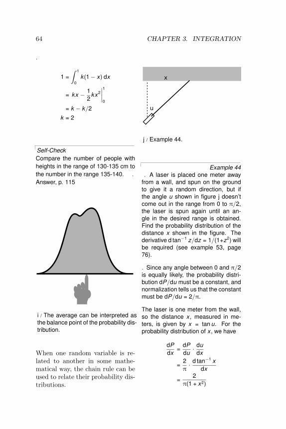
64 CHAPTER 3. INTEGRATION
.
1 =Z 1
0k (1− x) dx
= kx − 12
kx2˛10
= k − k/2
k = 2
Self-CheckCompare the number of people withheights in the range of 130-135 cm tothe number in the range 135-140. .
Answer, p. 115
i / The average can be interpreted asthe balance point of the probability dis-tribution.
When one random variable is re-lated to another in some mathe-matical way, the chain rule can beused to relate their probability dis-tributions.
j / Example 44.
Example 44. A laser is placed one meter away
from a wall, and spun on the groundto give it a random direction, but ifthe angle u shown in figure j doesn’tcome out in the range from 0 to π/2,the laser is spun again until an an-gle in the desired range is obtained.Find the probability distribution of thedistance x shown in the figure. Thederivative d tan−1 z/dz = 1/(1+z2) willbe required (see example 53, page76).
. Since any angle between 0 and π/2is equally likely, the probability distri-bution dP/du must be a constant, andnormalization tells us that the constantmust be dP/du = 2/π.
The laser is one meter from the wall,so the distance x , measured in me-ters, is given by x = tan u. For theprobability distribution of x , we have
dPdx
=dPdu· du
dx
=2π· d tan−1 x
dx
=2
π(1 + x2)
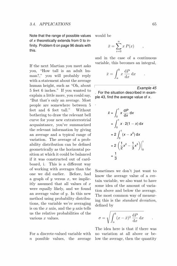
3.4. APPLICATIONS 65
Note that the range of possible valuesof x theoretically extends from 0 to in-finity. Problem 6 on page 96 deals withthis.
If the next Martian you meet asksyou, “How tall is an adult hu-man?,” you will probably replywith a statement about the averagehuman height, such as “Oh, about5 feet 6 inches.” If you wanted toexplain a little more, you could say,“But that’s only an average. Mostpeople are somewhere between 5feet and 6 feet tall.” Withoutbothering to draw the relevant bellcurve for your new extraterrestrialacquaintance, you’ve summarizedthe relevant information by givingan average and a typical range ofvariation. The average of a prob-ability distribution can be definedgeometrically as the horizontal po-sition at which it could be balancedif it was constructed out of card-board, i. This is a different wayof working with averages than theone we did earlier. Before, hada graph of y versus x, we implic-itly assumed that all values of xwere equally likely, and we foundan average value of y. In this newmethod using probability distribu-tions, the variable we’re averagingis on the x axis, and the y axis tellsus the relative probabilities of thevarious x values.
For a discrete-valued variable withn possible values, the average
would be
x =n∑i=0
x P (x) ,
and in the case of a continuousvariable, this becomes an integral,
x =∫ b
a
xdPdx
dx .
Example 45. For the situation described in exam-ple 43, find the average value of x .
.
x =Z 1
0x
dPdx
dx
=Z 1
0x · 2(1− x) dx
= 2Z 1
0(x − x2) dx
= 2„
12
x2 − 13
x3«˛1
0
=13
Sometimes we don’t just want toknow the average value of a cer-tain variable, we also want to havesome idea of the amount of varia-tion above and below the average.The most common way of measur-ing this is the standard deviation,defined by
σ =
√∫ b
a
(x− x)2dPdx
dx .
The idea here is that if there wasno variation at all above or be-low the average, then the quantity
66 CHAPTER 3. INTEGRATION
(x − x) would be zero wheneverdP/dx was nonzero, and the stan-dard deviation would be zero. Thereason for taking the square rootof the whole thing is so that theresult will have the same units asx.
Example 46. For the situation described in exam-ple 43, find the standard deviation ofx .
. The square of the standard deviationis
σ2 =Z 1
0(x − x)2 dP
dxdx
=Z 1
0(x − 1/3)2 · 2(1− x) dx
= 2Z 1
0
„−x3 +
53
x2 − 79
x +19
«dx
=1
18,
so the standard deviation is
σ =1√18
≈ 0.236
PROBLEMS 67
Problems1 Write a computer programsimilar to the one in example 37on page 58 to evaluate the definiteintegral ∫ 1
0
ex2
.
. Solution, p. 129
2 Evaluate the integral∫ 2π
0
sinx dx ,
and draw a sketch to explain whyyour result comes out the way itdoes. . Solution, p. 129
3 Sketch the graph that repre-sents the definite integral∫ 2
0
−x2 + 2x ,
and estimate the result roughlyfrom the graph. Then evaluate theintegral exactly, and check againstyour estimate.
. Solution, p. 130
4 Make a rough guess as to theaverage value of sinx for 0 < x <π, and then find the exact resultand check it against your guess.
. Solution, p. 131
5 Show that the mean value the-orem’s assumption of continuity isnecessary, by exhibiting a discon-tinuous function for which the the-orem fails. . Solution, p. 131
6 Show that the fundamentaltheorem of calculus’s assumption
of continuity for x is necessary, byexhibiting a discontinuous functionfor which the theorem fails.
. Solution, p. 131
7 Sketch the graphs of y = x2
and y =√x for 0 ≤ x ≤ 1. Graph-
ically, what relationship should ex-ist between the integrals
∫ 1
0x2 dx
and∫ 1
0
√x dx? Compute both in-
tegrals, and verify that the resultsare related in the expected way.
8 In a gasoline-burning car en-gine, the exploding air-gas mixturemakes a force on the piston, andthe force tapers off as the pistonexpands, allowing the gas to ex-pand. (a) In the approximationF = k/x, where x is the positionof the piston, find the work doneon the piston as it travels fromx = a to x = b, and show thatthe result only depends on the ra-tio b/a. This ratio is known asthe compression ratio of the en-gine. (b) A better approximation,which takes into account the cool-ing of the air-gas mixture as it ex-pands, is F = kx−1.4. Computethe work done in this case.
9 A certain variable x variesrandomly from -1 to 1, withprobability distribution dP/dx =k(1− x2
).
(a) Determine k from the require-ment of normalization.(b) Find the average value of x.(c) Find its standard deviation.
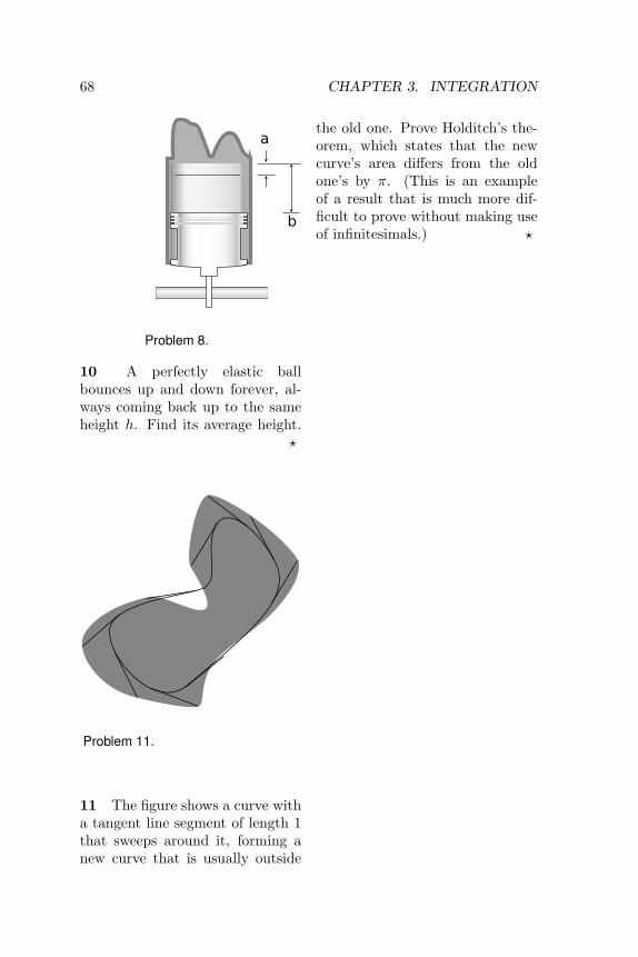
68 CHAPTER 3. INTEGRATION
Problem 8.
10 A perfectly elastic ballbounces up and down forever, al-ways coming back up to the sameheight h. Find its average height.
?
Problem 11.
11 The figure shows a curve witha tangent line segment of length 1that sweeps around it, forming anew curve that is usually outside
the old one. Prove Holditch’s the-orem, which states that the newcurve’s area differs from the oldone’s by π. (This is an exampleof a result that is much more dif-ficult to prove without making useof infinitesimals.) ?

4 Techniques4.1 Newton’s methodIn the 1958 science fiction novelHave Space Suit — WillTravel, by Robert Heinlein, Kipis a high school student who wantsto be an engineer, and his father istrying to convince him to stretchhimself more if he wants to get any-thing out of his education:
“Why did Van Buren fail of re-election? How do you extract thecube root of eighty-seven?”
Van Buren had been a president;that was all I remembered. But Icould answer the other one. “Ifyou want a cube root, you look ina table in the back of the book.”
Dad sighed. “Kip, do you thinkthat table was brought down fromon high by an archangel?”
We no longer use tables to com-pute roots, but how does a pocketcalculator do it? A techniquecalled Newton’s method allows usto calculate the inverse of any func-tion efficiently, including cases thataren’t preprogrammed into a cal-culator. In the example from thenovel, we know how to calculatethe function y = x3 fairly accu-rately and quickly for any givenvalue of x, but we want to turn theequation around and find x wheny = 87. We start with a roughmental guess: since 43 = 64 is a lit-
tle too small, and 53 = 125 is muchtoo big, we guess x ≈ 4.3. Test-ing our guess, we have 4.33 = 79.5.We want y to get bigger by 7.5, andwe can use calculus to find approx-imately how much bigger x needsto get in order to accomplish that:
∆x =∆x∆y
∆y
≈ dxdy
∆y
=∆y
dy/dx
=∆y3x2
=∆y3x2
= 0.14
Increasing our value of x to 4.3 +0.14 = 4.44, we find that 4.443 =87.5 is a pretty good approxima-tion to 87. If we need higher preci-sion, we can go through the processagain with ∆y = −0.5, giving
∆x ≈ ∆y3x2
= 0.14x = 4.43
x3 = 86.9 .
This second iteration gives an ex-cellent approximation.
Example 47. Figure 47 shows the astronomer Jo-hannes Kepler’s analysis of the motion
69

70 CHAPTER 4. TECHNIQUES
a / Example 47.
of the planets. The ellipse is the or-bit of the planet around the sun. Att = 0, the planet is at its closest ap-proach to the sun, A. At some latertime, the planet is at point B. The an-gle x (measured in radians) is definedwith reference to the imaginary circleencompassing the orbit. Kepler foundthe equation
2πtT
= x − e sin x ,
where the period, T , is the time re-quired for the planet to complete a fullorbit, and the eccentricity of the el-lipse, e, is a number that measureshow much it differs from a circle. Therelationship is complicated becausethe planet speeds up as it falls inwardtoward the sun, and slows down againas it swings back away from it.
The planet Mercury has e = 0.206.Find the angle x when Mercury hascompleted 1/4 of a period.
. We have
y = x − (0.206) sin x ,
and we want to find x when y =2π/4 = 1.57. As a first guess, we tryx = π/2 (90 degrees), since the ec-centricity of Mercury’s orbit is actuallymuch smaller than the example shownin the figure, and therefore the planet’sspeed doesn’t vary all that much as itgoes around the sun. For this value ofx we have y = 1.36, which is too smallby 0.21.
∆x ≈ ∆ydy/dx
=0.21
1− (0.206) cos x= 0.21
(The derivative dy/dx happens to be1 at x = π/2.) This gives a new valueof x , 1.57+.21=1.78. Testing it, wehave y = 1.58, which is correct towithin rounding errors after only oneiteration. (We were only supplied witha value of e accurate to three signifi-cant figures, so we can’t get a resultwith precision better than about thatlevel.)
4.2 Implicitdifferentiation
We can differentiate any functionthat is written as a formula, andfind a result in terms of a formula.However, sometimes the originalproblem can’t be written in anynice way as a formula. For exam-ple, suppose we want to find dy/dxin a case where the relationship be-tween x and y is given by the fol-lowing equation:
y7 + y = x7 + x2 .

4.3. TAYLOR SERIES 71
There is no equivalent of thequadratic formula for seventh-order polynomials, so we have noway to solve for one variable interms of the other in order to dif-ferentiate it. However, we can stillfind dy/dx in terms of x and y.Suppose we let x grow to x + dx.Then for example the x2 term willgrow to (x+ dx)2 = x+ 2dx+ dx2.The squared infinitesimal is negli-gible, so the increase in x2 was re-ally just 2dx, and we’ve really justcomputer the derivative of x2 withrespect to x and multiplied it bydx. In symbols,
d(x2) =d(x2)
dx· dx
= 2x dx .
That is, the change in x2 is 2xtimes the change in x. Doing thisto both sides of the original equa-tion, we have
d(y7 + y) = d(x7 + x2)
7y6 dy + 1 dy = 7x6 dx+ 2x dx
(7y6 + 1)dy = (7x6 + 2x)dx
dydx
=7x6 + 2x7y6 + 1
.
This still doesn’t give us a for-mula for the derivative in terms ofx alone, but it’s not entirely use-less. For instance, if we’re givena numerical value of x, we can al-ways use Newton’s method to findy, and then evaluate the derivative.
4.3 Taylor seriesIf you calculate e0.1 on your calcu-lator, you’ll find that it’s very closeto 1.1. This is because the tangentline at x = 0 on the graph of ex
has a slope of 1 (dex/dx = ex = 1at x = 0), and the tangent line isa good approximation to the expo-nential curve as long as we don’tget too far away from the point oftangency.
b / The function ex , andthe tangent line at x = 0.
How big is the error? Theactual value of e0.1 is1.10517091807565 . . ., whichdiffers from 1.1 by about 0.005.If we go farther from the pointof tangency, the approximationgets worse. At x = 0.2, the erroris about 0.021, which is aboutfour times bigger. In other words,doubling x seems to roughlyquadruple the error, so the erroris proportional to x2; it seems tobe about x2/2. Well, if we wanta handy-dandy, super-accurateestimate of ex for small values of
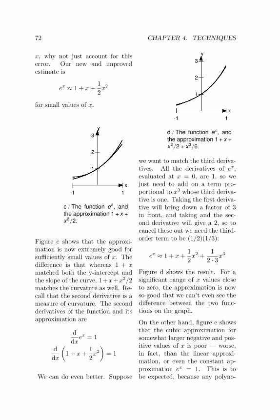
72 CHAPTER 4. TECHNIQUES
x, why not just account for thiserror. Our new and improvedestimate is
ex ≈ 1 + x+12x2
for small values of x.
c / The function ex , andthe approximation 1 + x +x2/2.
Figure c shows that the approxi-mation is now extremely good forsufficiently small values of x. Thedifference is that whereas 1 + xmatched both the y-intercept andthe slope of the curve, 1+x+x2/2matches the curvature as well. Re-call that the second derivative is ameasure of curvature. The secondderivatives of the function and itsapproximation are
ddxex = 1
ddx
(1 + x+
12x2
)= 1
We can do even better. Suppose
d / The function ex , andthe approximation 1 + x +x2/2 + x3/6.
we want to match the third deriva-tives. All the derivatives of ex,evaluated at x = 0, are 1, so wejust need to add on a term pro-portional to x3 whose third deriva-tive is one. Taking the first deriva-tive will bring down a factor of 3in front, and taking and the sec-ond derivative will give a 2, so tocancel these out we need the third-order term to be (1/2)(1/3):
ex ≈ 1 + x+12x2 +
12 · 3
x3
Figure d shows the result. For asignificant range of x values closeto zero, the approximation is nowso good that we can’t even see thedifference between the two func-tions on the graph.
On the other hand, figure e showsthat the cubic approximation forsomewhat larger negative and pos-itive values of x is poor — worse,in fact, than the linear approxi-mation, or even the constant ap-proximation ex = 1. This is tobe expected, because any polyno-

4.3. TAYLOR SERIES 73
mial will blow up to either posi-tive or negative infinity as x ap-proaches negative infinity, whereasthe function ex is supposed to getvery close to zero for large negativex. The idea here is that derivativesare local things: they only measurethe properties of a function veryclose to the point at which they’reevaluated, and they don’t necessar-ily tell us anything about points faraway.
e / The function ex , and the approxi-mation 1 + x + x2/2 + x3/6, on a widerscale.
It’s a remarkable fact, then, thatby taking enough terms in a poly-nomial approximation, we can al-ways get as good an approximationto ex as necessary — it’s just thata large number of terms may berequired for large values of x. Inother words, the infinite series
1 + x+12x2 +
12 · 3
x3 + . . .
always gives exactly ex. But whatis the pattern here that would al-lows us to figure out, say, thefourth-order and fifth-order termsthat were swept under the rugwith the symbol “. . . ”? Let’s dothe fifth-order term as an example.The point of adding in a fifth-orderterm is to make the fifth derivativeof the approximation equal to thefifth derivative of ex, which is 1.The first, second, . . . derivatives ofx5 are
ddxx5 = 5x4
d2
dx2x5 = 5 · 4x3
d3
dx3x5 = 5 · 4 · 3x2
d4
dx4x5 = 5 · 4 · 3 · 2x
d5
dx5x5 = 5 · 4 · 3 · 2 · 1
The notation for a product like 1 ·2 · . . . · n is n!, read “n factorial.”So to get a term for our polynomialwhose fifth derivative is 1, we needx5/5!. The result for the infiniteseries is
ex =∞∑n=0
xn
n!,
where the special case of 0! = 1 isassumed.1 This is called the Tay-lor series for ex, evaluated aroundx = 0, and it’s true, although I
1This makes sense, because, for exam-ple, 4!=5!/5, 3!=4!/4, etc., so we shouldhave 0!=1!/1.
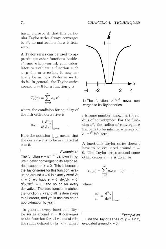
74 CHAPTER 4. TECHNIQUES
haven’t proved it, that this partic-ular Taylor series always convergesto ex, no matter how far x is fromzero.
A Taylor series can be used to ap-proximate other functions besidesex, and when you ask your calcu-lator to evaluate a function suchas a sine or a cosine, it may ac-tually be using a Taylor series todo it. In general, the Taylor seriesaround x = 0 for a function y is
T0(x) =∞∑n=0
anxn ,
where the condition for equality ofthe nth order derivative is
an =1n!
dnydxn
∣∣∣∣x=0
.
Here the notation |x=0 means thatthe derivative is to be evaluated atx = 0.
Example 48The function y = e−1/x2
, shown in fig-ure f, never converges to its Taylor se-ries, except at x = 0. This is becausethe Taylor series for this function, eval-uated around x = 0 is exactly zero! Atx = 0, we have y = 0, dy/dx = 0,d2y/dx2 = 0, and so on for everyderivative. The zero function matchesthe function y (x) and all its derivativesto all orders, and yet is useless as anapproximation to y (x).
In general, every function’s Tay-lor series around x = 0 convergesto the function for all values of x inthe range defined by |x| < r, where
f / The function e−1/x2never con-
verges to its Taylor series.
r is some number, known as the ra-dius of convergence. For the func-tion ex, the radius of convergencehappens to be infinite, whereas fore−1/x2
it’s zero.
A function’s Taylor series doesn’thave to be evaluated around x =0. The Taylor series around someother center x = c is given by
Tc(x) =∞∑n=0
an(x− c)n ,
where
ann!
=dnydxn
∣∣∣∣x=c
.
Example 49. Find the Taylor series of y = sin x ,evaluated around x = 0.
4.3. TAYLOR SERIES 75
. The first few derivatives are
ddx
sin x = cos x
d2
dx2 sin x = − sin x
d3
dx3 sin x = − cos x
d4
dx4 sin x = sin x
d5
dx5 sin x = cos x
We can see that there will be a cy-cle of sin, cos, − sin, and − cos, re-peating indefinitely. Evaluating thesederivatives at x = 0, we have 0, 1, 0,−1, . . . . All the even-order terms ofthe series are zero, and all the odd-order terms are ±1/n!. The result is
sin x = x − 13!
x3 +15!
x5 − . . . .
The linear term is the familiar small-angle approximation sin x ≈ x .
The radius of convergence of this se-ries turns out to be infinite. Intuitivelythe reason for this is that the factori-als grow extremely rapidly, so that thesuccessive terms in the series even-tually start diminish quickly, even forlarge values of x .
Example 50. Find the Taylor series of y = 1/(1−x)around x = 0, and see what you cansay about its radius of convergence.
. Rewriting the function as y = (1 −x)−1 and applying the chain rule, we
have
y |x=0 = 1
dydx
˛x=0
= (1− x)−2˛x=0
= 1
d2ydx2
˛x=0
= 2(1− x)−3˛x=0
= 2
d3ydx3
˛x=0
= 2 · 3(1− x)−4˛x=0
= 2 · 3
. . .
The pattern is that the nth derivativeis n!. The Taylor series therefore hasan = n!/n! = 1:
11− x
= 1 + x + x2 + x3 + . . .
The radius of convergence of this se-ries definitely can’t be greater than 1,since for x = 1 the series is 1 + 1 +1 + . . ., which grows indefinitely with-out ever converging to a specific num-ber. Likewise for x = −1 the seriesbecomes 1 − 1 + 1 − 1 + . . ., whichoscillates back and forth rather thanconverging. Intuitively we can see acouple of hints as to why this hap-pens: (1) The function 1/(1 − x) it-self misbehaves at x = 1, blowing upto infinity; (2) The only way a seriescan get closer and closer to a finitevalue is if the absolute values of theterms decrease, and decrease suffi-ciently rapidly. But the coefficients an
of this Taylor series don’t decreasewith n, so so the only way the abso-lute values of the terms can decreaseis for |x | < 1.
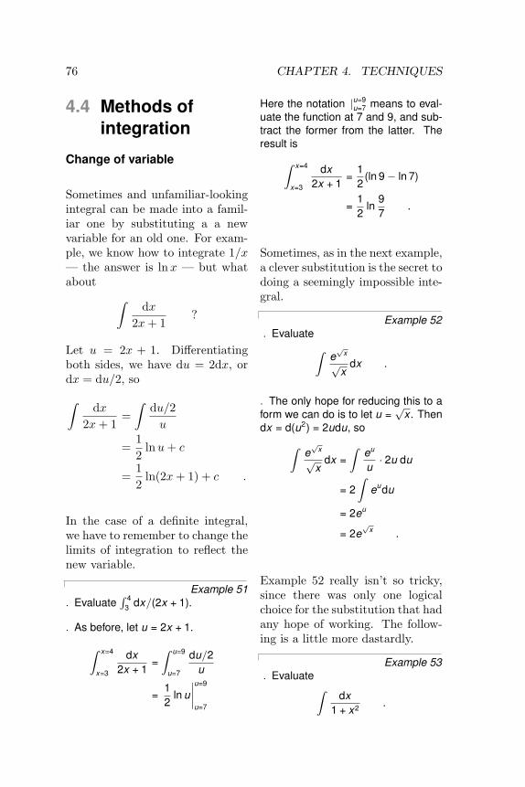
76 CHAPTER 4. TECHNIQUES
4.4 Methods ofintegration
Change of variable
Sometimes and unfamiliar-lookingintegral can be made into a famil-iar one by substituting a a newvariable for an old one. For exam-ple, we know how to integrate 1/x— the answer is lnx — but whatabout ∫
dx2x+ 1
?
Let u = 2x + 1. Differentiatingboth sides, we have du = 2dx, ordx = du/2, so∫
dx2x+ 1
=∫
du/2u
=12
lnu+ c
=12
ln(2x+ 1) + c .
In the case of a definite integral,we have to remember to change thelimits of integration to reflect thenew variable.
Example 51. Evaluate
R 43 dx/(2x + 1).
. As before, let u = 2x + 1.Z x=4
x=3
dx2x + 1
=Z u=9
u=7
du/2u
=12
ln u˛u=9
u=7
Here the notation |u=9u=7 means to eval-
uate the function at 7 and 9, and sub-tract the former from the latter. Theresult isZ x=4
x=3
dx2x + 1
=12
(ln 9− ln 7)
=12
ln97
.
Sometimes, as in the next example,a clever substitution is the secret todoing a seemingly impossible inte-gral.
Example 52. EvaluateZ
e√
x
√x
dx .
. The only hope for reducing this to aform we can do is to let u =
√x . Then
dx = d(u2) = 2udu, soZe√
x
√x
dx =Z
eu
u· 2u du
= 2Z
eudu
= 2eu
= 2e√
x .
Example 52 really isn’t so tricky,since there was only one logicalchoice for the substitution that hadany hope of working. The follow-ing is a little more dastardly.
Example 53. Evaluate Z
dx1 + x2 .

4.4. METHODS OF INTEGRATION 77
. The substitution that works is x =tan u. First let’s see what this doesto the expression 1 + x2. The familiaridentity
sin2 u + cos2 u = 1 ,
when divided by cos2 u, gives
tan2 u + 1 = sec2 u ,
so 1 + x2 becomes sec2 u. But differ-entiating both sides of x = tan u gives
dx = dhsin u(cos u)−1
i= (d sin u)(cos u)−1
+ (sin u)dh(cos u)−1
i=“
1 + tan2 u”
du
= sec2 u du ,
so the integral becomesZdx
1 + x2 =Z
sec2 udusec2 u
= u + c
= tan−1 x + c .
What mere mortal would everhave suspected that the substitu-tion x = tanu was the one thatwas needed in example 53? Onepossible answer is to give up anddo the integral on a computer:
Integrate(x) 1/(1+x^2)ArcTan(x)
Another possible answer is thatyou can usually smell the pos-sibility of this type of substitu-tion, involving a trig function,
when the thing to be integratedcontains something reminiscent ofthe Pythagorean theorem, as sug-gested by figure g. The 1+x2 lookslike what you’d get if you had aright triangle with legs 1 and x,and were using the Pythagoreantheorem to find its hypotenuse.
g / The substitution x =tan u.
Example 54. Evaluate
Rdx/√
1− x2.
. The√
1− x2 looks like what you’dget if you had a right triangle withhypotenuse 1 and a leg of length x ,and were using the Pythagorean the-orem to find the other leg, as in fig-ure h. This motivates us to try thesubstitution x = cos u, which givesdx = − sin u du and
√1− x2 =√
1− cos2 u = sin u. The result isZdx√
1− x2=Z− sin u du
sin u
= u + c
= cos−1 x .
h / The substitution x =cos u.

78 CHAPTER 4. TECHNIQUES
Integration by parts
Figure i shows a technique calledintegration by parts. If the inte-gral
∫vdu is easier than the inte-
gral∫udv, then we can calculate
the easier one, and then by sim-ple geometry determine the one wewanted. Identifying the large rect-angle that surrounds both shadedareas, and the small white rectan-gle on the lower left, we have∫u dv =(area of large rectangle)
− (area of small rectangle)∫v du .
i / Integration by parts.
In the case of an indefinite integral,we have a similar relationship de-
rived from the product rule:
d(uv) = u dv + v duu dv = d(uv)− v du
Integrating both sides, we have thefollowing relation.
Integration by parts∫u dv = uv −
∫v du .
Since a definite integral can al-ways be done by evaluating an in-definite integral at its upper andlower limits, one usually uses thisform. Integrals don’t usually comeprepackaged in a form that makesit obvious that you should use inte-gration by parts. What the equa-tion for integration by parts tellsus is that if we can split up theintegrand into two factors, one ofwhich (the dv) we know how tointegrate, we have the option ofchanging the integral into a newform in which that factor becomesits integral, and the other fac-tor becomes its derivative. If wechoose the right way of splitting upthe integrand into parts, the resultcan be a simplification.
Example 55. Evaluate Z
x cos x dx
. There are two obvious possibilitiesfor splitting up the integrand into fac-
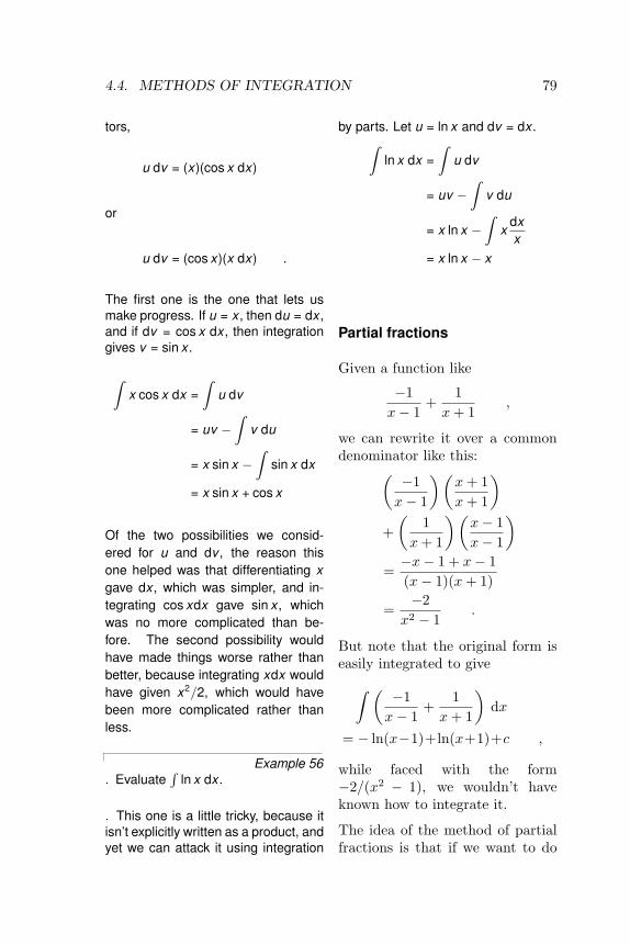
4.4. METHODS OF INTEGRATION 79
tors,
u dv = (x)(cos x dx)
or
u dv = (cos x)(x dx) .
The first one is the one that lets usmake progress. If u = x , then du = dx ,and if dv = cos x dx , then integrationgives v = sin x .
Zx cos x dx =
Zu dv
= uv −Z
v du
= x sin x −Z
sin x dx
= x sin x + cos x
Of the two possibilities we consid-ered for u and dv , the reason thisone helped was that differentiating xgave dx , which was simpler, and in-tegrating cos xdx gave sin x , whichwas no more complicated than be-fore. The second possibility wouldhave made things worse rather thanbetter, because integrating xdx wouldhave given x2/2, which would havebeen more complicated rather thanless.
Example 56. Evaluate
Rln x dx .
. This one is a little tricky, because itisn’t explicitly written as a product, andyet we can attack it using integration
by parts. Let u = ln x and dv = dx .Zln x dx =
Zu dv
= uv −Z
v du
= x ln x −Z
xdxx
= x ln x − x
Partial fractions
Given a function like
−1x− 1
+1
x+ 1,
we can rewrite it over a commondenominator like this:(
−1x− 1
)(x+ 1x+ 1
)+(
1x+ 1
)(x− 1x− 1
)=−x− 1 + x− 1(x− 1)(x+ 1)
=−2
x2 − 1.
But note that the original form iseasily integrated to give∫ (
−1x− 1
+1
x+ 1
)dx
= − ln(x−1)+ln(x+1)+c ,
while faced with the form−2/(x2 − 1), we wouldn’t haveknown how to integrate it.
The idea of the method of partialfractions is that if we want to do
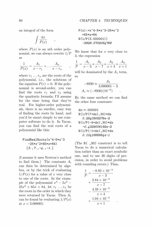
80 CHAPTER 4. TECHNIQUES
an integral of the form∫dxP (x)
,
where P (x) is an nth order poly-nomial, we can always rewrite 1/Pas
1P (x)
=A1
x− r1+ . . .
Anx− rn
,
where r1 . . . rn are the roots of thepolynomial, i.e., the solutions ofthe equation P (r) = 0. If the poly-nomial is second-order, you canfind the roots r1 and r2 usingthe quadratic formula; I’ll assumefor the time being that they’rereal. For higher-order polynomi-als, there is no surefire, easy wayof finding the roots by hand, andyou’d be smart simply to use com-puter software to do it. In Yacas,you can find the real roots of apolynomial like this:
FindRealRoots(x^4-5*x^3-25*x^2+65*x+84){3.,7.,-4.,-1.}
(I assume it uses Newton’s methodto find them.) The constants Aican then be determined by alge-bra, or by the trick of evaluating1/P (x) for a value of x very closeto one of the roots. In the exam-ple of the polynomial x4 − 5x3 −25x2 + 65x + 84, let r1 . . . r4 bethe roots in the order in which theywere returned by Yacas. Then A1
can be found by evaluating 1/P (x)at x = 3.000001:
P(x):=x^4-5*x^3-25*x^2+65*x+84
N(1/P(3.000001))-8928.5702094768
We know that for x very close to3, the expression
1P
=A1
x− 3+
A2
x− 7+
A3
x+ 4+
A4
x+ 1
will be dominated by the A1 term,so
−8930 ≈ A1
3.000001− 3A1 ≈ (−8930)(10−6) .
By the same method we can findthe other four constants:
dx:=.000001N(1/P(7+dx),30)*dx
0.2840908276e-2
N(1/P(-4+dx),30)*dx-0.4329006192e-2
N(1/P(-1+dx),30)*dx0.1041666664e-1
(The N( ,30) construct is to tellYacas to do a numerical calcula-tion rather than an exact symbolicone, and to use 30 digits of pre-cision, in order to avoid problemswith rounding errors.) Thus,
1P
=−8.93× 10⁻³
x− 3
+2.84× 10⁻³
x− 7
− 4.33× 10⁻³
x+ 4
+1.04× 10⁻²
x+ 1.

4.4. METHODS OF INTEGRATION 81
The desired integral is∫dxP (x)
= −8.93× 10⁻³ ln(x− 3)
+ 2.84× 10⁻³ ln(x− 7)
− 4.33× 10⁻³ ln(x+ 4)
+ 1.04× 10⁻² ln(x+ 1)+ c .
There are some possible complica-tions: (1) The same factor may oc-cur more than once, as in x3−5x2+7x−3 = (x−1)(x−1)(x−3). In thisexample, we have to look for an an-swer of the form A/(x−1)+B/(x−1)2 +C/(x− 3), the solution being−.25/(x−1)−.5/(x−1)2+.25/(x−3). (2) The roots may be complex.This is no show-stopper if you’reusing computer software that han-dles complex numbers gracefully.(You can choose a c that makes theresult real.) In fact, as discussed insection 5.3, some beautiful thingscan happen with complex roots.But as an alternative, any polyno-mial with real coefficients can befactored into linear and quadraticfactors with real coefficients. Foreach quadratic factor Q(x), wethen have a partial fraction of theform (A+Bx)/Q(x), where A andB can be determined by algebra.In Yacas, this can be done usingthe Apart function.
Example 57. Evaluate the integralZ
dx(x4 − 8 ∗ x3 + 8 ∗ x2 − 8 ∗ x + 7
using the method of partial fractions.
. First we use Yacas to look for realroots of the polynomial:
FindRealRoots(x^4-8*x^3
+8*x^2-8*x+7)
{1.,7.}
Unfortunately this polynomial seemsto have only two real roots; the restare complex. We can divide out thefactor (x − 1)(x − 7), but that stillleaves us with a second-order polyno-mial, which has no real roots. One ap-proach would be to factor the polyno-mial into the form (x − 1)(x − 7)(x −p)(x −q), where p and q are complex,as in section 5.3. Instead, let’s use Ya-cas to expand the integrand in termsof partial fractions:
Apart(1/(x^4-8*x^3
+8*x^2-8*x+7))
((2*x)/25+3/50)/(x^2+1)
+1/(300*(x-7))
+(-1)/(12*(x-1))
We can now rewrite the integral likethis:
225
Zx dx
x2 + 1
+3
50
Zdx
x2 + 1
+1
300
Zdx
x − 7
− 112
Zdx
x − 1

82 CHAPTER 4. TECHNIQUES
which we can evaluate as follows:
125
ln(x2 + 1)
+3
50tan−1 x
+1
300ln(x − 7)
− 112
ln(x − 1)
+c
In fact, Yacas should be able to dothe whole integral for us from scratch,but it’s best to understand how thesethings work under the hood, and toavoid being completely dependent onone particular piece of software. Asan illustration of this gem of wisdom,I found that when I tried to make Ya-cas evaluate the integral in one gulp,it choked because the calculation be-came too complicated! Because I un-derstood the ideas behind the proce-dure, I was still able to get a resultthrough a mixture of computer calcu-lations and working it by hand. Some-one who didn’t have the knowledge ofthe technique might have tried the in-tegral using the software, seen it fail,and concluded, incorrectly, that the in-tegral was one that simply couldn’t bedone. A computer is no substitute forunderstanding.

PROBLEMS 83
Problems
1 Graph the function y = ex −7x and get an approximate idea ofwhere any of its zeroes are (i.e., forwhat values of x we have y(x) = 0).Use Newton’s method to find thezeroes to three significant figures ofprecision.
2 The relationship between x andy is given by xy = sin y + x2y2.(a) Use Newton’s method to findthe nonzero solution for y whenx = 3. Answer: y = 0.2231(b) Find dy/dx in terms of x andy, and evaluate the derivative atthe point on the curve you found inpart a. Answer: dy/dx = −0.0379Based on an example by Craig B.
Watkins.
3 Find the Taylor series expan-sion of ln(1+x) around x = 0, anduse it to evaluate ln 1.776 to foursignificant figures of precision.
4 In free fall, the acceleration willnot be exactly constant, due to airresistance. For example, a sky-diver does not speed up indefi-nitely until opening her chute, butrather approaches a certain maxi-mum velocity at which the upwardforce of air resistance cancels outthe force of gravity. If an object isdropped from a height h, and thetime it takes to reach the ground isused to measure the acceleration ofgravity, g, then the relative error in
the result due to air resistance is2
E =g − gvacuum
g
= 1− 2b
ln2(eb +
√e2b − 1
) ,
where b = h/A, and A is a constantthat depends on the size, shape,and mass of the object, and thedensity of the air. (For a sphere ofmass m and diameter d droppingin air, A = 4.11m/d2. Cf. problem15, p. 51.) Evaluate the constantand linear terms of the Taylor se-ries for the function E(b).
5 Suppose you want to evaluate∫dx
1 + sin 2x,
and you’ve found∫dx
1 + sinx= − tan
(π4− x
2
)in a table of integrals. Use achange of variable to find the an-swer to the original problem.
6 Evaluate∫sinxdx
1 + cosx.
7 Evaluate∫sinxdx
1 + cos2 x.
8 Evaluate∫xe−x
2dx .
2Jan Benacka and Igor Stubna, ThePhysics Teacher, 43 (2005) 432.

84 CHAPTER 4. TECHNIQUES
9 Evaluate∫xex dx .
10 Use integration by parts toevaluate the following integrals.∫
sin−1 x dx∫cos−1 x dx∫tan−1 x dx
11 Evaluate∫x2 sinx dx .
Hint: Use integration by partsmore than once.
12 Evaluate∫dx
x2 − x− 6.
13 Evaluate∫dx
x3 + 3x2 − 4.
14 Evaluate∫dx
x3 − x2 + 4x− 4.

5 Complex numbertechniques
5.1 Review ofcomplexnumbers
For a more detailed treatment ofcomplex numbers, see ch. 3 ofJames Nearing’s free book athttp://www.physics.miami.edu/nearing/mathmethods/.
a / Visualizing complex numbers aspoints in a plane.
We assume there is a number, i,such that i2 = −1. The squareroots of −1 are then i and −i. (Inelectrical engineering work, wherei stands for current, j is sometimesused instead.) This gives rise toa number system, called the com-plex numbers, containing the real
b / Addition of complex numbers isjust like addition of vectors, althoughthe real and imaginary axes don’t ac-tually represent directions in space.
numbers as a subset. Any com-plex number z can be written inthe form z = a + bi, where a andb are real, and a and b are thenreferred to as the real and imagi-nary parts of z. A number witha zero real part is called an imag-inary number. The complex num-bers can be visualized as a plane,figure a, with the real number lineplaced horizontally like the x axisof the familiar x−y plane, and theimaginary numbers running alongthe y axis. The complex num-bers are complete in a way that thereal numbers aren’t: every nonzerocomplex number has two squareroots. For example, 1 is a real
85
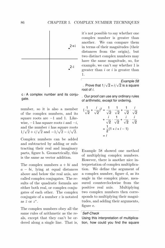
86 CHAPTER 5. COMPLEX NUMBER TECHNIQUES
c / A complex number and its conju-gate.
number, so it is also a memberof the complex numbers, and itssquare roots are −1 and 1. Like-wise, −1 has square roots i and −i,and the number i has square roots1/√
2 + i/√
2 and −1/√
2− i/√
2.
Complex numbers can be addedand subtracted by adding or sub-tracting their real and imaginaryparts, figure b. Geometrically, thisis the same as vector addition.
The complex numbers a + bi anda − bi, lying at equal distancesabove and below the real axis, arecalled complex conjugates. The re-sults of the quadratic formula areeither both real, or complex conju-gates of each other. The complexconjugate of a number z is notatedas z or z∗.
The complex numbers obey all thesame rules of arithmetic as the re-als, except that they can’t be or-dered along a single line. That is,
it’s not possible to say whether onecomplex number is greater thananother. We can compare themin terms of their magnitudes (theirdistances from the origin), buttwo distinct complex numbers mayhave the same magnitude, so, forexample, we can’t say whether 1 isgreater than i or i is greater than1.
Example 58. Prove that 1/
√2 + i/
√2 is a square
root of i .
.Our proof can use any ordinary rulesof arithmetic, except for ordering.
(1√2
+i√2
)2 =1√2· 1√
2+
1√2· i√
2
+i√2· 1√
2+
i√2· i√
2
=12
(1 + i + i − 1)
= i
Example 58 showed one methodof multiplying complex numbers.However, there is another nice in-terpretation of complex multiplica-tion. We define the argument ofa complex number, figure d, as itsangle in the complex plane, mea-sured counterclockwise from thepositive real axis. Multiplyingtwo complex numbers then corre-sponds to multiplying their magni-tudes, and adding their arguments,figure e.
Self-CheckUsing this interpretation of multiplica-tion, how could you find the square

5.1. REVIEW OF COMPLEX NUMBERS 87
d / A complex number can be de-scribed in terms of its magnitude andargument.
roots of a complex number? .
Answer, p. 115
Example 59The magnitude |z| of a complex num-ber z obeys the identity |z|2 = zz.To prove this, we first note that z hasthe same magnitude as z, since flip-ping it to the other side of the real axisdoesn’t change its distance from theorigin. Multiplying z by z gives a re-sult whose magnitude is found by mul-tiplying their magnitudes, so the mag-nitude of zz must therefore equal |z|2.Now we just have to prove that zz is apositive real number. But if, for exam-ple, z lies counterclockwise from thereal axis, then z lies clockwise fromit. If z has a positive argument, thenz has a negative one, or vice-versa.The sum of their arguments is there-fore zero, so the result has an argu-ment of zero, and is on the positivereal axis. 1
1I cheated a little. If z’s argument is
e / The argument of uv is the sum ofthe arguments of u and v .
This whole system was built upin order to make every numberhave square roots. What aboutcube roots, fourth roots, and soon? Does it get even more weirdwhen you want to do those as well?No. The complex number systemwe’ve already discussed is sufficientto handle all of them. The nicestway of thinking about it is in termsof roots of polynomials. In thereal number system, the polyno-mial x2− 1 has two roots, i.e., twovalues of x (plus and minus one)that we can plug in to the polyno-mial and get zero. Because it hasthese two real roots, we can rewritethe polynomial as (x − 1)(x + 1).However, the polynomial x2+1 hasno real roots. It’s ugly that in thereal number system, some second-
30 degrees, then we could say z’s was -30,but we could also call it 330. That’s OK,because 330+30 gives 360, and an argu-ment of 360 is the same as an argumentof zero.

88 CHAPTER 5. COMPLEX NUMBER TECHNIQUES
order polynomials have two roots,and can be factored, while otherscan’t. In the complex number sys-tem, they all can. For instance,x2 + 1 has roots i and −i, and canbe factored as (x − i)(x + i). Ingeneral, the fundamental theoremof algebra states that in the com-plex number system, any nth-orderpolynomial can be factored com-pletely into n linear factors, andwe can also say that it has n com-plex roots, with the understand-ing that some of the roots may bethe same. For instance, the fourth-order polynomial x4 + x2 can befactored as (x− i)(x+ i)(x−0)(x−0), and we say that it has fourroots, i, −i, 0, and 0, two of whichhappen to be the same. This is asensible way to think about it, be-cause in real life, numbers are al-ways approximations anyway, andif we make tiny, random changes tothe coefficients of this polynomial,it will have four distinct roots, ofwhich two just happen to be veryclose to zero. I’ve given a proof ofthe fundamental theorem of alge-bra on page 112.
5.2 Euler’s formula
Having expanded our horizons toinclude the complex numbers, it’snatural to want to extend func-tions we knew and loved from theworld of real numbers so that theycan also operate on complex num-bers. The only really natural wayto do this in general is to use Tay-lor series. A particularly beautiful
thing happens with the functionsex, sinx, and cosx:
ex = 1 +12!x2 +
13!x3 + . . .
cosx = 1− 12!x2 +
14!x4 − . . .
sinx = x− 13!x3 +
15!x5 − . . .
If x = iφ is an imaginary number,we have
eiφ = cosφ+ i sinφ ,
a result known as Euler’s formula.The geometrical interpretation inthe complex plane is shown in fig-ure f.
f / The complex number eiφ lies on theunit circle.
Although the result may seem likesomething out of a freak show atfirst, applying the definition2 of the
2See page 111 for an explanation of

5.2. EULER’S FORMULA 89
exponential function makes it clearhow natural it is:
ex = limn→∞
(1 +
x
n
)n.
When x = iφ is imaginary, thequantity (1 + iφ/n) represents anumber lying just above 1 in thecomplex plane. For large n, (1 +iφ/n) becomes very close to theunit circle, and its argument is thesmall angle φ/n. Raising this num-ber to the nth power multiplies itsargument by n, giving a numberwith an argument of φ.
g / Leonhard Euler(1707-1783)
Euler’s formula is used frequentlyin physics and engineering.
Example 60. Write the sine and cosine functionsin terms of exponentials.
. Euler’s formula for x = −iφ givescos φ− i sin φ, since cos(−θ) = cos θ,
where this definition comes from and whyit makes sense.
and sin(−θ) = − sin θ.
cos x =eix + e−ix
2
sin x =eix − e−ix
2i
Example 61. Evaluate Z
ex cos xdx
. This seemingly impossible integralbecomes easy if we rewrite the cosinein terms of exponentials:
Zex cos xdx
=Z
ex„
eix + e−ix
2
«dx
=12
Z(e(1+i)x + e(1−i)x ) dx
=12
„e(1+i)x
1 + i+
e(1−i)x
1− i
«+ c
Since this result is the integral of areal-valued function, we’d like it to bereal, and in fact it is, since the first andsecond terms are complex conjugatesof one another. If we wanted to, wecould use Euler’s theorem to convertit back to a manifestly real result.3
3In general, the use of complex num-ber techniques to do an integral could re-sult in a complex number, but that com-plex number would be a constant, whichcould be subsumed within the usual con-stant of integration.
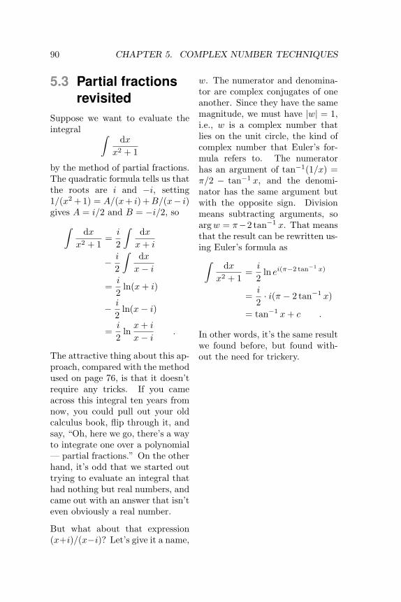
90 CHAPTER 5. COMPLEX NUMBER TECHNIQUES
5.3 Partial fractionsrevisited
Suppose we want to evaluate theintegral ∫
dxx2 + 1
by the method of partial fractions.The quadratic formula tells us thatthe roots are i and −i, setting1/(x2 + 1) = A/(x+ i) +B/(x− i)gives A = i/2 and B = −i/2, so∫
dxx2 + 1
=i
2
∫dxx+ i
− i
2
∫dxx− i
=i
2ln(x+ i)
− i
2ln(x− i)
=i
2lnx+ i
x− i.
The attractive thing about this ap-proach, compared with the methodused on page 76, is that it doesn’trequire any tricks. If you cameacross this integral ten years fromnow, you could pull out your oldcalculus book, flip through it, andsay, “Oh, here we go, there’s a wayto integrate one over a polynomial— partial fractions.” On the otherhand, it’s odd that we started outtrying to evaluate an integral thathad nothing but real numbers, andcame out with an answer that isn’teven obviously a real number.
But what about that expression(x+i)/(x−i)? Let’s give it a name,
w. The numerator and denomina-tor are complex conjugates of oneanother. Since they have the samemagnitude, we must have |w| = 1,i.e., w is a complex number thatlies on the unit circle, the kind ofcomplex number that Euler’s for-mula refers to. The numeratorhas an argument of tan−1(1/x) =π/2 − tan−1 x, and the denomi-nator has the same argument butwith the opposite sign. Divisionmeans subtracting arguments, soargw = π−2 tan−1 x. That meansthat the result can be rewritten us-ing Euler’s formula as∫
dxx2 + 1
=i
2ln ei(π−2 tan−1 x)
=i
2· i(π − 2 tan−1 x)
= tan−1 x+ c .
In other words, it’s the same resultwe found before, but found with-out the need for trickery.

PROBLEMS 91
Problems1 Find arg i, arg(−i), and arg 37,where arg z denotes the argumentof the complex number z.
2 Visualize the following multi-plications in the complex planeusing the interpretation of mul-tiplication in terms of multiply-ing magnitudes and adding argu-ments: (i)(i) = −1, (i)(−i) = 1,(−i)(−i) = −1.
3 If we visualize z as a point inthe complex plane, how should wevisualize −z?
4 Find four different complexnumbers z such that z4 = 1.
5 Compute the following:
|1 + i| , arg(1 + i) ,∣∣∣∣ 11 + i
∣∣∣∣ , arg(
11 + i
),
11 + i
6 Write the function tanx interms of complex exponentials.
7 Evaluate∫dx
x3 − x2 + 4x− 4.
8 Evaluate∫e−ax cos bx dx .

92 CHAPTER 5. COMPLEX NUMBER TECHNIQUES
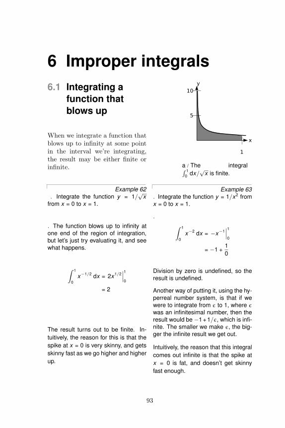
6 Improper integrals6.1 Integrating a
function thatblows up
When we integrate a function thatblows up to infinity at some pointin the interval we’re integrating,the result may be either finite orinfinite.
Example 62. Integrate the function y = 1/
√x
from x = 0 to x = 1.
. The function blows up to infinity atone end of the region of integration,but let’s just try evaluating it, and seewhat happens.
Z 1
0x−1/2 dx = 2x1/2
˛10
= 2
The result turns out to be finite. In-tuitively, the reason for this is that thespike at x = 0 is very skinny, and getsskinny fast as we go higher and higherup.
a / The integralR 10 dx/
√x is finite.
Example 63. Integrate the function y = 1/x2 fromx = 0 to x = 1.
. Z 1
0x−2 dx = −x−1
˛10
= −1 +10
Division by zero is undefined, so theresult is undefined.
Another way of putting it, using the hy-perreal number system, is that if wewere to integrate from ε to 1, where ε
was an infinitesimal number, then theresult would be −1 + 1/ε, which is infi-nite. The smaller we make ε, the big-ger the infinite result we get out.
Intuitively, the reason that this integralcomes out infinite is that the spike atx = 0 is fat, and doesn’t get skinnyfast enough.
93
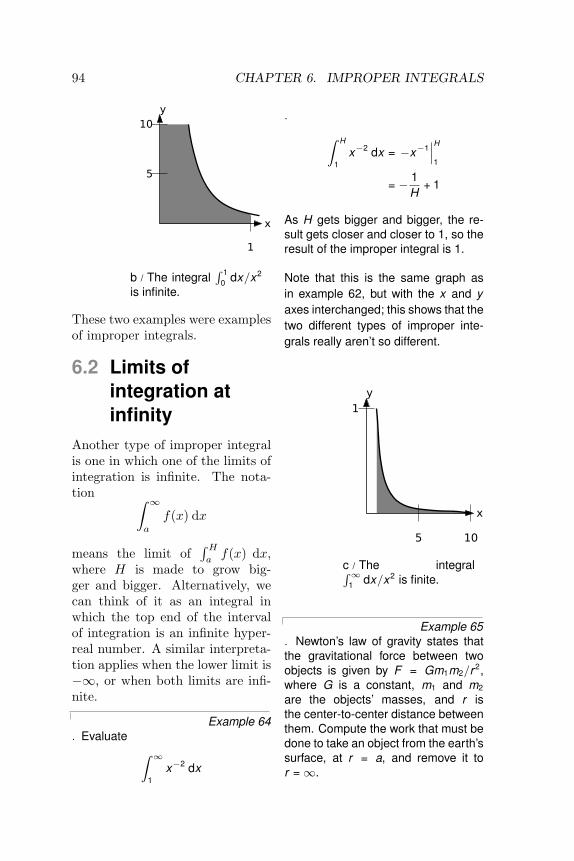
94 CHAPTER 6. IMPROPER INTEGRALS
b / The integralR 1
0 dx/x2
is infinite.
These two examples were examplesof improper integrals.
6.2 Limits ofintegration atinfinity
Another type of improper integralis one in which one of the limits ofintegration is infinite. The nota-tion ∫ ∞
a
f(x) dx
means the limit of∫Haf(x) dx,
where H is made to grow big-ger and bigger. Alternatively, wecan think of it as an integral inwhich the top end of the intervalof integration is an infinite hyper-real number. A similar interpreta-tion applies when the lower limit is−∞, or when both limits are infi-nite.
Example 64. Evaluate Z ∞
1x−2 dx
. Z H
1x−2 dx = −x−1
˛H1
= − 1H
+ 1
As H gets bigger and bigger, the re-sult gets closer and closer to 1, so theresult of the improper integral is 1.
Note that this is the same graph asin example 62, but with the x and yaxes interchanged; this shows that thetwo different types of improper inte-grals really aren’t so different.
c / The integralR∞1 dx/x2 is finite.
Example 65. Newton’s law of gravity states thatthe gravitational force between twoobjects is given by F = Gm1m2/r 2,where G is a constant, m1 and m2
are the objects’ masses, and r isthe center-to-center distance betweenthem. Compute the work that must bedone to take an object from the earth’ssurface, at r = a, and remove it tor =∞.

6.2. LIMITS OF INTEGRATION AT INFINITY 95
.
W =Z ∞
a
Gm1m2
r 2 dr
= Gm1m2
Z ∞a
r−2 dr
= −Gm1m2 r−1˛∞a
=Gm1m2
a
The answer is inversely proportionalto a. In other words, if we were able tostart from higher up, less work wouldhave to be done.

96 CHAPTER 6. IMPROPER INTEGRALS
Problems1 Integrate∫ ∞
0
e−xdx ,
or show that it diverges.
2 Integrate∫ ∞1
dxx
,
or show that it diverges.
3 Integrate∫ 1
0
dxx
,
or show that it diverges.
4 Integrate∫ ∞0
e−x cosx dx
or show that it diverges.
5 Prove that∫ ∞0
e−ex
dx
converges, but don’t evaluate it.
6 (a) Verify that the probabilitydistribution dP/dx given in exam-ple 44 on page 64 is properly nor-malized.(b) Find the average value of x, orshow that it diverges.(c) Find the standard deviation ofx, or show that it diverges.
7 Prove∫ ∞0
e−xxn dx = n! .
?

7 Iterated integrals7.1 Integrals inside
integralsIn various applications, you needto do integrals stuck inside otherintegrals. These are known as it-erated integrals, or double inte-grals, triple integrals, etc. Simi-lar concepts crop up all the timeeven when you’re not doing cal-culus, so let’s start by imaginingsuch an example. Suppose youwant to count how many squaresthere are on a chess board, and youdon’t know how to multiply eighttimes eight. You could start fromthe upper left, count eight squaresacross, then continue with the sec-ond row, and so on, until youhow counted every square, givingthe result of 64. In slightly moreformal mathematical language, wecould write the following recipe:for each row, r, from 1 to 8, con-sider the columns, c, from 1 to 8,and add one to the count for eachone of them. Using the sigma no-tation, this becomes
8∑r=1
8∑c=1
1 .
If you’re familiar with computerprogramming, then you can thinkof this as a sum that could becalculated using a loop nested in-side another loop. To evaluate theresult (again, assuming we don’t
know how to multiply, so we haveto use brute force), we can firstevaluate the inside sum, whichequals 8, giving
8∑r=1
8 .
Notice how the “dummy” variablec has disappeared. Finally we dothe outside sum, over r, and findthe result of 64.
Now imagine doing the same thingwith the pixels on a TV screen.The electron beam sweeps acrossthe screen, painting the pixels ineach row, one at a time. This is re-ally no different than the exampleof the chess board, but because thepixels are so small, you normallythink of the image on a TV screenas continuous rather than discrete.This is the idea of an integral incalculus. Suppose we want to findthe area of a rectangle of width aand height b, and we don’t knowthat we can just multiply to getthe area ab. The brute force wayto do this is to break up the rect-angle into a grid of infinitesimallysmall squares, each having widthdx and height dy, and therefore theinfinitesimal area dA = dxdy. Forconvenience, we’ll imagine that therectangle’s lower left corner is atthe origin. Then the area is given
97

98 CHAPTER 7. ITERATED INTEGRALS
by this integral:
area =∫ b
y=0
∫ a
x=0
dA
=∫ b
y=0
∫ a
x=0
dx dy
Notice how the leftmost integralsign, over y, and the rightmostdifferential, dy, act like bookends,or the pieces of bread on a sand-wich. Inside them, we have the in-tegral sign that runs over x, andthe differential dx that matches iton the right. Finally, on the inner-most layer, we’d normally have thething we’re integrating, but here’sit’s 1, so I’ve omitted it. Writ-ing the lower limits of the integralswith x = and y = helps to keepit straight which integral goes withwith differential. The result is
area =∫ b
y=0
∫ a
x=0
dA
=∫ b
y=0
∫ a
x=0
dx dy
=∫ b
y=0
(∫ a
x=0
dx)
dy
=∫ b
y=0
a dy
= a
∫ b
y=0
dy
= ab .
Area of a triangle Example 66. Find the area of a 45-45-90 right tri-angle having legs a.
. Let the triangle’s hypotenuse runfrom the origin to the point (a, a), and
let its legs run from the origin to (0, a),and then to (a, a). In other words, thetriangle sits on top of its hypotenuse.Then the integral can be set up thesame way as the one before, but for aparticular value of y , values of x onlyrun from 0 (on the y axis) to y (on thehypotenuse). We then have
area =Z a
y=0
Z y
x=0dA
=Z a
y=0
Z y
x=0dx dy
=Z a
y=0
„Z y
x=0dx«
dy
=Z a
y=0y dy
=12
a2
Note that in this example, because theupper end of the x values dependson the value of y , it makes a differ-ence which order we do the integralsin. The x integral has to be on the in-side, and we have to do it first.
Volume of a cube Example 67. Find the volume of a cube with sidesof length a.
. This is a three-dimensional example,so we’ll have integrals nested threedeep, and the thing we’re integratingis the volume dV = dxdydz.
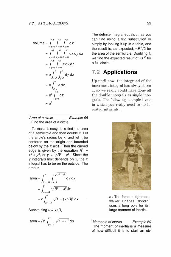
7.2. APPLICATIONS 99
volume =Z a
z=0
Z a
y=0
Z a
x=0dV
=Z a
z=0
Z a
y=0
Z a
x=0dx dy dz
=Z a
z=0
Z a
y=0a dy dz
= aZ a
z=0
Z a
y=0dy dz
= aZ a
z=0a dz
= a2Z a
z=0dz
= a3
Area of a circle Example 68. Find the area of a circle.
. To make it easy, let’s find the areaof a semicircle and then double it. Letthe circle’s radius be r , and let it becentered on the origin and boundedbelow by the x axis. Then the curvededge is given by the equation R2 =x2 + y2, or y =
√R2 − x2. Since the
y integral’s limit depends on x , the xintegral has to be on the outside. Thearea is
area =Z r
x=−R
Z √R2−x2
y=0dy dx
=Z r
x=−R
pR2 − x2dx
= rZ r
x=−R
p1− (x/R)2 dx .
Substituting u = x/R,
area = R2Z 1
u=−1
p1− u2 du
The definite integral equals π, as youcan find using a trig substitution orsimply by looking it up in a table, andthe result is, as expected, πR2/2 forthe area of the semicircle. Doubling it,we find the expected result of πR2 fora full circle.
7.2 ApplicationsUp until now, the integrand of theinnermost integral has always been1, so we really could have done allthe double integrals as single inte-grals. The following example is onein which you really need to do it-erated integrals.
a / The famous tightropewalker Charles Blondinuses a long pole for itslarge moment of inertia.
Moments of inertia Example 69The moment of inertia is a measure
of how difficult it is to start an ob-

100 CHAPTER 7. ITERATED INTEGRALS
ject rotating (or stop it). For example,tightrope walkers carry long poles be-cause they want something with a bigmoment of inertia. The moment of in-ertia is defined by I =
RR2dm, where
dm is the mass of an infinitesimallysmall portion of the object, and R isthe distance from the axis of rotation.
To start with, let’s do an example thatdoesn’t require iterated integrals. Let’scalculate the moment of inertia of athin rod of mass M and length L abouta line perpendicular to the rod andpassing through its center.
I =Z
R2dm
=Z L/2
−L/2x2 M
Ldx
[r = |x |, so R2 = x2]
=1
12ML2
Now let’s do one that requires iter-ated integrals: the moment of inertiaof a cube of side b, for rotation aboutan axis that passes through its centerand is parallel to four of its faces.
Let the origin be at the center of thecube, and let x be the rotation axis.
I =Z
R2dm
= ρ
ZR2dV
= ρ
Z b/2
b/2
Z b/2
b/2
Z b/2
b/2
“y2 + z2
”dx dy dz
= ρbZ b/2
b/2
Z b/2
b/2
“y2 + z2
”dy dz
The fact that the last step is a trivial in-tegral results from the symmetry of the
problem. The integrand of the remain-ing double integral breaks down intotwo terms, each of which depends ononly one of the variables, so we breakit into two integrals,
I =ρbZ b/2
b/2
Z b/2
b/2y2dy dz
+ ρbZ b/2
b/2
Z b/2
b/2z2dy dz
which we know have identical results.We therefore only need to evaluateone of them and double the result:
I = 2ρbZ b/2
b/2
Z b/2
b/2z2dy d z
= 2ρb2Z b/2
b/2z2dz
=16
ρb5
=16
Mb2

7.3. POLAR COORDINATES 101
7.3 Polar coordinates
b / Rene Descartes(1596-1650)
Philosopher and mathematicianRene Descartes originated the ideaof describing plane geometry using(x, y) coordinates measured froma pair of perpendicular coordinateaxes. These rectangular coordi-nates are known as Cartesian co-ordinates, in his honor.
c / Polar coordinates.
As a logical extension of Descartes’idea, one can find different ways ofdefining coordinates on the plane,such as the polar coordinates in fig-
ure c. In polar coordinates, the dif-ferential of area, figure d can bewritten as da = R dR dφ. Theidea is that since dR and dφ are in-finitesimally small, the shaded areain the figure is very nearly a rect-angle, measuring dR is one dimen-sion and R dφ in the other. (Thelatter follows from the definition ofradian measure.)
d / The differential ofarea in polar coordinates
Example 70. A disk has mass M and radius b.Find its moment of inertia for rota-tion about the axis passing perpendic-ularly through its center.
.
I =Z
R2dM
=Z
R2 dMda
da
=Z
R2 Mπb2 da
=M
πb2
Z b
R=0
Z 2π
φ=0R2 · R dφ dR
=M
πb2
Z b
R=0R3Z 2π
φ=0dφ dR
=2Mb2
Z b
R=0R3 dR
=Mb4
2
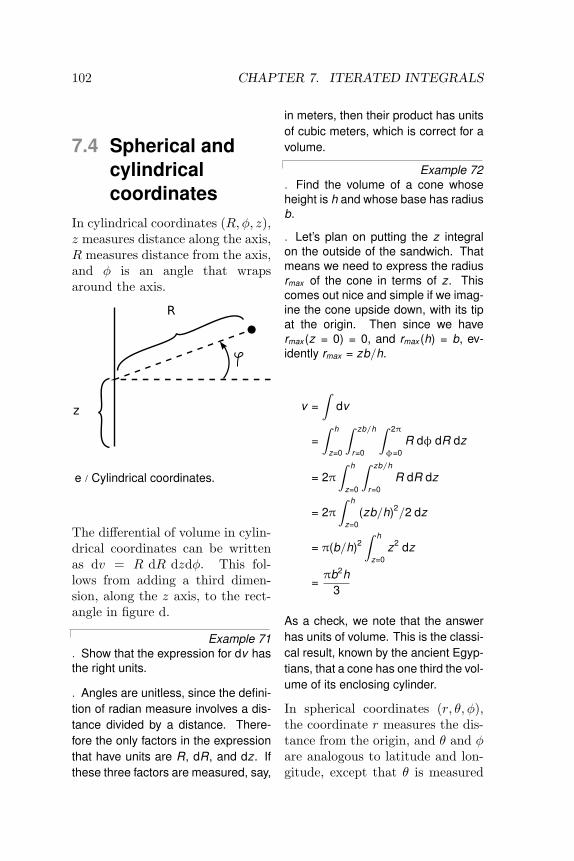
102 CHAPTER 7. ITERATED INTEGRALS
7.4 Spherical andcylindricalcoordinates
In cylindrical coordinates (R,φ, z),z measures distance along the axis,R measures distance from the axis,and φ is an angle that wrapsaround the axis.
e / Cylindrical coordinates.
The differential of volume in cylin-drical coordinates can be writtenas dv = R dR dzdφ. This fol-lows from adding a third dimen-sion, along the z axis, to the rect-angle in figure d.
Example 71. Show that the expression for dv hasthe right units.
. Angles are unitless, since the defini-tion of radian measure involves a dis-tance divided by a distance. There-fore the only factors in the expressionthat have units are R, dR, and dz. Ifthese three factors are measured, say,
in meters, then their product has unitsof cubic meters, which is correct for avolume.
Example 72. Find the volume of a cone whoseheight is h and whose base has radiusb.
. Let’s plan on putting the z integralon the outside of the sandwich. Thatmeans we need to express the radiusrmax of the cone in terms of z. Thiscomes out nice and simple if we imag-ine the cone upside down, with its tipat the origin. Then since we havermax (z = 0) = 0, and rmax (h) = b, ev-idently rmax = zb/h.
v =Z
dv
=Z h
z=0
Z zb/h
r=0
Z 2π
φ=0R dφ dR dz
= 2π
Z h
z=0
Z zb/h
r=0R dR dz
= 2π
Z h
z=0(zb/h)2/2 dz
= π(b/h)2Z h
z=0z2 dz
=πb2h
3
As a check, we note that the answerhas units of volume. This is the classi-cal result, known by the ancient Egyp-tians, that a cone has one third the vol-ume of its enclosing cylinder.
In spherical coordinates (r, θ,φ),the coordinate r measures the dis-tance from the origin, and θ and φare analogous to latitude and lon-gitude, except that θ is measured

7.4. SPHERICAL AND CYLINDRICAL COORDINATES 103
down from the pole rather thanfrom the equator.
f / Spherical coordinates.
The differential of volume inspherical coordinates is dv =r2 sin θ dr dθ dφ.
Example 73. Find the volume of a sphere.
.
v =Z
dv
=Z π
θ=0
Z r=b
r=0
Z 2π
φ=0r 2 sin θ dφ dr dθ
= 2π
Z π
θ=0
Z r=b
r=0r 2 sin θ dr dθ
= 2π · b3
3
Z π
θ=0sin θ dθ
=4πb3
3

104 CHAPTER 7. ITERATED INTEGRALS
Problems1 Pascal’s snail (named afterEtienne Pascal, father of BlaisePascal) is the shape shown in thefigure, defined by R = b(1 + cos θ)in polar coordinates.(a) Make a rough visual estimateof its area from the figure.(b) Find its area exactly, and checkagainst your result from part a.(c) Show that your answer has theright units. [Thompson, 1919]
Problem 1: Pascal’s snail with b = 1.
2 A cone with a curved base isdefined by r ≤ b and θ ≤ π/4 inspherical coordinates.(a) Find its volume.(b) Show that your answer has theright units.
3 Find the moment of inertia ofa sphere for rotation about an axispassing through its center.
4 A jump-rope swinging in circleshas the shape of a sine function.
Find the volume enclosed by theswinging rope, in terms of the ra-dius b of the circle at the rope’sfattest point, and the straight-linedistance ` between the ends.
5 A curvy-sided cone is defined incylindrical coordinates by 0 ≤ z ≤h and R ≤ kz2. (a) What unitsare implied for the constant k? (b)Find the volume of the shape. (c)Check that your answer to b hasthe right units.
6 The discovery of nuclear fis-sion was originally explained bymodeling the atomic nucleus as adrop of liquid. Like a water bal-loon, the drop could spin or vi-brate, and if the motion becamesufficiently violent, the drop couldsplit in half — undergo fission. Itwas later learned that even thenuclei in matter under ordinaryconditions are often not sphericalbut deformed, typically with anelongated ellipsoidal shape like anAmerican football. One simpleway of describing such a shape iswith the equation
r ≤ b[1 + c(cos2 θ − k)] ,
where c = 0 for a sphere, c > 0 foran elongated shape, and c < 0 fora flattened one. Usually for nucleiin ordinary matter, c ranges fromabout 0 to +0.2. The constant kis introduced because without it, achange in c would entail not justa change in the shape of the nu-cleus, but a change in its volumeas well. Observations show, on thecontrary, that the nuclear fluid, is
PROBLEMS 105
highly incompressible, just like or-dinary water, so the volume of thenucleus is not expected to changesignificantly, even in violent pro-cesses like fission. Calculate thevolume of the nucleus, throwingaway terms of order c2 or higher,and show that k = 1/3 is requiredin order to keep the volume con-stant.
7 This problem is a continua-tion of problem 6, and assumes theresult of that problem is alreadyknown. The nucleus 168Er has thetype of elongated ellipsoidal shapedescribed in that problem, withc > 0. Its mass is 2.8 × 10⁻²⁵ kg,it is observed to have a momentof inertia of 2.62 × 10−54 kg ·m2
for end-over-end rotation, and itsshape is believed to be describedby b ≈ 6 × 10⁻¹⁵ m and c ≈ 0.2.Assuming that it rotated rigidly,the usual equation for the momentof inertia could be applicable, butit may rotate more like a water bal-loon, in which case its moment ofinertia would be significantly lessbecause not all the mass would ac-tually flow. Test which type of ro-tation it is by calculating its mo-ment of inertia for end-over-end ro-tation and comparing with the ob-served moment of inertia. ?

106 CHAPTER 7. ITERATED INTEGRALS

A DetoursFormal definition of the tangent line
Let (a, b) be a point on the graph of the function x(t). A line `(t)through this point is said not to cut through the graph if there existssome real number d > 0 such that x(t)− `(t) has the same sign for all tbetween a− d and a+ d. The line is said to be the tangent line at thispoint if it is the only line through this point that doesn’t cut throughthe graph.1
Derivatives of polynomials
We want to prove that the derivative of tk is ktk−1. It suffices to provethat the derivative equals k when evaluated at t = 1, since we canthen apply the kind of scaling argument2 used on page 14 to show thatthe derivative of t2/2 was t. The proposed tangent line at (1, 1) hasthe equation ` = k(t − 1) + 1, so what we need to prove is that thepolynomial tk − [k(t − 1) + 1] is greater than or equal to zero in somefinite region around t = 1.
First, let’s change variables to u = t − 1. Then the polynomial inquestion becomes P (u) = (u+1)k− (ku+1), and we want to prove thatit’s nonnegative in some region around u = 0. (We assume k ≥ 2, sincewe’ve already found the derivatives in the cases of k = 0 and 1, and inthose cases P (u) is identically zero.)
Now the last two terms in the binomial series for (u + 1)k are just kuand 1, so P (u) is a polynomial whose lowest-order term is a u2 term.Also, all the nonzero coefficients of the polynomial are positive, so P ispositive for u ≥ 0.
To complete the proof we only need to establish that P is also positivefor sufficiently small negative values of u. For negative u, the even-order
1As an exception, there are cases in which the function is smooth and well-behavedthroughout a certain region, but has no tangent line according to this definition at oneparticular point. For example, the function x(t) = t3 has tangent lines everywhereexcept at t = 0, which is an inflection point (p. 18). In such cases, we fill in the“gap tooth” in the derivative function in the obvious way.
2In the special case of t = 0, the scaling argument doesn’t work. For even k, itcan be easily verified that the derivative at t = 0 equals zero. For odd k, we have tofill in the “gap tooth” as described in the preceding footnote.
107

108 A Detours
terms of P are positive, and the odd-order terms negative. To make theidea clear, consider the k = 5 case, where P (u) = u5 + 5u4 + 10u3 +10u2. The idea is to pair off each positive term with the negative oneimmediately to its left. Although the coefficient of the negative termmay, in general, be greater than the coefficient of the positive termwith which we’ve paired it, a property of the binomial coefficients isthat the ratio of successive coefficients is never greater than k. Thusfor −1/k < u < 0, each positive term is guaranteed to dominate thenegative term immediately to its left.
Details of the proof of the derivative of the sine function
Some ideas in this proof are due to Jerome Keisler.
On page 25, I computed
dx = sin(t+ dt)− sin t ,= sin t cos dt
+ cos t sin dt− sin t≈ cos t dt .
Here I’ll prove that the error introduced by the small-angle approxima-tions really is of order dt2. We have
sin(t+ dt) = sin t+ cos tdt− E ,
where the error E introduced by the approximations is
E = sin t(1− cos dt)+ cos t(dt− sin dt) .
a / Geometrical interpre-tation of the error term.
Let the radius of the circle in figure a be one, so AD is cos dt and CD issin dt. The area of the shaded pie slice is dt/2, and the area of triangle

109
ABC is sin dt/2, so the error made in the approximation sin dt ≈ dtequals twice the area of the dish shape formed by line BC and arc BC.Therefore dt−sin dt is less than the area of rectangle CEBD. But CEBDhas both an infinitesimal width and an infinitesimal height, so this erroris of no more than order dt2.
For the approximation cos dt ≈ 1, the error (represented by BD) is1 − cos dt = 1 −
√1− sin2 dt, which is less than 1 −
√1− dt2, since
sin dt < dt. Therefore this error is of order dt2.
The transfer principle applied to functions
On page 30, I told you not to worry about whether it was legitimateto apply familiar functions like x2,
√x, sinx, cosx, and ex to hyperreal
numbers. But since you’re reading this, you’re obviously in need of morereassurance.
For some of these functions, the transfer principle straightforwardlyguarantees that they work for hyperreals, have all the familiar proper-ties, and can be computed in the same way. For example, the followingstatement is in a suitable form to have the transfer principle applied toit: For any real number x, x · x ≥ 0. Changing “real” to “hyperreal,”we find out that the square of a hyperreal number is greater than orequal to zero, just like the square of a real number. Writing it as x2
or calling it a square is just a matter of notation and terminology. Thesame applies to this statement: For any real number x ≥ 0, there existsa real number y such that y2 = x. Applying the transfer function to ittells us that square roots can be defined for the hyperreals as well.
There’s a problem, however, when we get to functions like sinx andex. If you look up the definition of the sine function in a trigonometrytextbook, it will be defined geometrically, as the ratio of the lengths oftwo sides of a certain triangle. The transfer principle doesn’t apply togeometry, only to arithmetic. It’s not even obvious intuitively that itmakes sense to define a sine function on the hyperreals. In an applicationlike the differentiation of the sine function on page 25, we only had totake sines of hyperreal numbers that were infinitesimally close to realnumbers, but if the sine is going to be a full-fledged function defined onthe hyperreals, then we should be allowed, for example, to take the sineof an infinite number. What would that mean? If you take the sine of anumber like a million or a billion on your calculator, you just get someapparently random result between −1 and 1. The sine function wigglesback and forth indefinitely as x gets bigger and bigger, never settlingdown to any specific limiting value. Apparently we could have sinH = 1
110 A Detours
for a particular infinite H, and then sin(H+π/2) = 0, sin(H+π) = −1,. . .
It turns out that the moral equivalent of the transfer function can in-deed be applied to any function on the reals, yielding a function thatis in some sense its natural “big brother” on the the hyperreals, butthe consequences can be either disturbing or exhilirating dependingon your tastes. For example, consider the function [x] that takes areal number x and rounds it down to the greatest integer that is lessthan or equal to to x, e.g., [3] = 3, and [π] = 3. This function, likeany other real function, can be extended to the hyperreals, and thatmeans that we can define the hyperintegers, the set of hyperreals thatsatisfy [x] = x. The hyperintegers include the integers as a subset,but they also include infinite numbers. This is likely to seem magi-cal, or even unreasonable, if we come at the hyperreals from the ax-iomatic point of view, as in this book and Keisler’s more detailed treat-ment in Elementary Calculus: An Approach Using Infinitesimals, http://www.math.wisc.edu/~keisler/calc.html. The extension of func-tions to the hyperreals seems much more natural in an alternative, con-structive approach, which is explained admirably in an online article athttp://mathforum.org/dr.math/faq/analysis_hyperreals.html.
Proof of the chain rule
In the statement of the chain rule on page 33, I followed my usualcustom of writing derivatives as dy/dx, when actually the derivative isthe standard part, st(dy/dx). In more rigorous notation, the chain ruleshould be stated like this:
st(
dzdx
)= st
(dzdy
)st(
dydx
).
The transfer principle allows us to rewrite the left-hand side asst[(dz/dy)(dy/dx)], and then we can get the desired result using theidentity st(ab) = st(a)st(b).
Derivative of ex
All of the reasoning on page 34 would have applied equally well to anyother exponential function with a different base, such as 2x or 10x.Those functions would have different values of c, so if we want to deter-mine the value of c for the base-e case, we need to bring in the definitionof e, or of the exponential function ex, somehow.

111
We can take the definition of ex to be
ex = limn→∞
(1 +
x
n
)n.
The idea behind this relation is similar to the idea of compound interest.If the interest rate is 10%, compounded annually, then x = 0.1, andthe balance grows by a factor (1 + x) = 1.1 in one year. If, instead,we want to compound the interest monthly, we can set the monthlyinterest rate to 0.1/12, and then the growth of the balance over a yearis (1+x/12)12 = 1.1047, which is slightly larger because the interest fromthe earlier months itself accrues interest in the later months. Continuingthis limiting process, we find e1.1 = 1.1052.
If n is large, then we have a good approximation to the base-e ex-ponential, so let’s differentiate this finite-n approximation and try tofind an approximation to the derivative of ex. The chain rule tells isthat the derivative of (1 + x/n)n is the derivative of the raising-to-the-nth-power function, multiplied by the derivative of the inside stuff,d(1 + x/n)/dx = 1/n. We then have
d(1 + x
n
)ndx
=[n(
1 +x
n
)n−1]· 1n
=(
1 +x
n
)n−1
.
But evaluating this at x = 0 simply gives 1, so at x = 0, the approxi-mation to the derivative is exactly 1 for all values of n — it’s not evennecessary to imagine going to larger and larger values of n. This estab-lishes that c = 1, so we have
dex
dx= ex
for all values of x.
Proof of the fundamental theorem of calculus
There are three parts to the proof: (1) Take the equation that statesthe fundamental theorem, differentiate both sides with respect to b, andshow that they’re equal. (2) Show that continuous functions with equalderivatives must be essentially the same function, except for an additiveconstant. (3) Show that the constant in question is zero.
1. By the definition of the indefinite integral, the derivative of x(b)−x(a)with respect to b equals x(b). We have to establish that this equals the

112 A Detours
following:
ddb
∫ b
a
x(t)dt = st1db
[∫ b+db
a
x(t)dt−∫ b
a
x(t)dt
]
= st1db
∫ b+db
b
x(t)dt
= st1db
limH→∞
H∑i=0
x(b + i db/H)dbH
= st limH→∞
1H
H∑i=0
x(b + i db/H)
Since x is continuous, all the values of x occurring inside the sum candiffer only infinitesimally from x(b). Therefore the quantity inside thelimit differs only infinitesimally from x(b), and the standard part of itslimit must be x(b).3
2. Suppose f and g are two continuous functions whose derivatives areequal. Then d = f − g is a continuous function whose derivative is zero.But the only continuous function with a derivative of zero is a constant,so f and g differ by at most an additive constant.
3. I’ve established that the derivatives with respect to b of x(b)− x(a)and
∫ baxdt are the same, so they differ by at most an additive constant.
But at b = a, they’re both zero, so the constant must be zero.
Proof of the mean value theorem
Suppose that the mean value theorem is violated. Let L by the set of allx in the interval from a to b such that y(x) < y, and likewise let M bethe set with y(x) > y. If the theorem is violated, then the union of thesetwo sets covers the entire interval from a to b. Neither one can be empty;if, for example, M was empty, then we would have y < y everywhereand also
∫ bay =
∫ bay, but it follows directly from the definition of the
definite integral that when one function is less than another, its integralis also less than the other’s. Since y takes on values less than and greaterthan y, it follows from the intermediate value theorem that y takes onthe value y somewhere (intuitively, at a boundary between L and M).
Proof of the fundamental theorem of algebra
3If you don’t want to use infinitesimals, then you can express the derivative as alimit, and in the final step of the argument use the mean value theorem, introducedlater in the chapter.
113
Theorem: In the complex number system, an nth-order polynomial hasexactly n roots, i.e., it can be factored into the form P (z) = (z−a1)(z−a2) . . . (z − an), where the ai are complex numbers.
Proof: The proofs in the cases of n = 0 and 1 are trivial, so our strategyis to reduce higher-n cases to lower ones. If an nth-degree polynomial Phas at least one root, a, then we can always reduce it to a polynomial ofdegree n− 1 by dividing it by (z − a). Therefore the theorem is provedby induction provided that we can show that every polynomial of degreegreater than zero has at least one root.
Suppose, on the contrary, that there is an nth order polynomial P (z),with n > 0, that has no roots at all. Then |P (z)| must have someminimum value, which is achieved at z = zo. (Polynomials don’t haveasymptotes, so the minimum really does have to occur for some specific,finite zo.) To make things more simple and concrete, we can constructanother polynomial Q(z) = P (z+zo)/P (zo), so that |Q| has a minimumvalue of 1, achieved at Q(0) = 1. This means that Q’s constant term is1. What about its other terms? Let Q(z) = 1+c1z+. . .+cnzn. Supposec1 was nonzero. Then for infinitesimally small values of z, the terms oforder z2 and higher would be negligible, and we could make Q(z) bea real number less than one by an appropriate choice of z’s argument.Therefore c1 must be zero. But that means that if c2 is nonzero, then forinfinitesimally small z, the z2 term dominates the z3 and higher terms,and again this would allow us to make Q(z) be real and less than onefor appropriately chosen values of z. Continuing this process, we findthat Q(z) has no terms at all beyond the constant term, i.e., Q(z) = 1.This contradicts the assumption that n was greater than zero, so we’veproved by contradiction that there is no P with the properties claimed.

114 A Detours

B Answers and solutions
Answers to Self-Checks
Answers to self-checks for chapter 3
page 64, self-check 1:
The area under the curve from 130 to 135 cm is about 3/4 of a rectangle.The area from 135 to 140 cm is about 1.5 rectangles. The number of peo-ple in the second range is about twice as much. We could have convertedthese to actual probabilities (1 rectangle = 5 cm×0.005 cm−1 = 0.025),but that would have been pointless, because we were just going to com-pare the two areas.
Answers to self-checks for chapter 5
page 86, self-check 1: Say we’re looking for u =√z, i.e., we want a
number u that, multiplied by itself, equals z. Multiplication multipliesthe magnitudes, so the magnitude of u can be found by taking the squareroot of the magnitude of z. Since multiplication also adds the argumentsof the numbers, squaring a number doubles its argument. Therefore wecan simply divide the argument of z by two to find the argument ofu. This results in one of the square roots of z. There is another one,which is −u, since (−u)2 is the same as u2. This may seem a little odd:if u was chosen so that doubling its argument gave the argument of z,then how can the same be true for −u? Well for example, suppose theargument of z is 4 ◦. Then arg u = 2 ◦, and arg(−u) = 182 ◦. Doubling182 gives 364, which is actually a synonym for 4 degrees.
115

116 B Answers and solutions
Solutions to homework problems
Solutions for chapter 1
page 21, problem 1:
The tangent line has to pass through the point (3,9), and it also seems,at least approximately, to pass through (1.5,0). This gives it a slope of(9− 0)/(3− 1.5) = 9/1.5 = 6, and that’s exactly what 2t is at t = 3.
a / Problem 1.
page 21, problem 2:
The tangent line has to pass through the point (0, sin(e0)) = (0, 0.84),and it also seems, at least approximately, to pass through (-1.6,0). Thisgives it a slope of (0.84− 0)/(0− (−1.6)) = 0.84/1.6 = 0.53. The moreaccurate result given in the problem can be found using the methods ofchapter 2.
b / Problem 2.
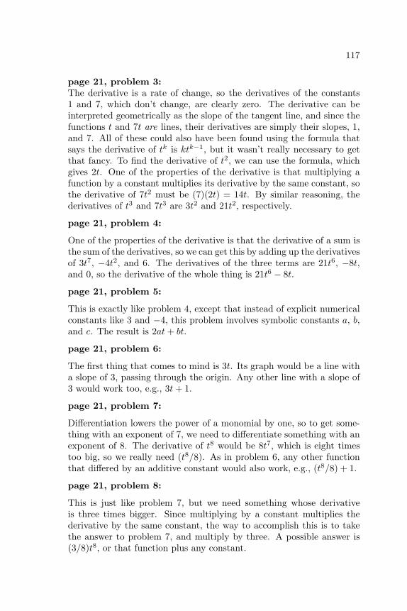
117
page 21, problem 3:The derivative is a rate of change, so the derivatives of the constants1 and 7, which don’t change, are clearly zero. The derivative can beinterpreted geometrically as the slope of the tangent line, and since thefunctions t and 7t are lines, their derivatives are simply their slopes, 1,and 7. All of these could also have been found using the formula thatsays the derivative of tk is ktk−1, but it wasn’t really necessary to getthat fancy. To find the derivative of t2, we can use the formula, whichgives 2t. One of the properties of the derivative is that multiplying afunction by a constant multiplies its derivative by the same constant, sothe derivative of 7t2 must be (7)(2t) = 14t. By similar reasoning, thederivatives of t3 and 7t3 are 3t2 and 21t2, respectively.
page 21, problem 4:
One of the properties of the derivative is that the derivative of a sum isthe sum of the derivatives, so we can get this by adding up the derivativesof 3t7, −4t2, and 6. The derivatives of the three terms are 21t6, −8t,and 0, so the derivative of the whole thing is 21t6 − 8t.
page 21, problem 5:
This is exactly like problem 4, except that instead of explicit numericalconstants like 3 and −4, this problem involves symbolic constants a, b,and c. The result is 2at+ bt.
page 21, problem 6:
The first thing that comes to mind is 3t. Its graph would be a line witha slope of 3, passing through the origin. Any other line with a slope of3 would work too, e.g., 3t+ 1.
page 21, problem 7:
Differentiation lowers the power of a monomial by one, so to get some-thing with an exponent of 7, we need to differentiate something with anexponent of 8. The derivative of t8 would be 8t7, which is eight timestoo big, so we really need (t8/8). As in problem 6, any other functionthat differed by an additive constant would also work, e.g., (t8/8) + 1.
page 21, problem 8:
This is just like problem 7, but we need something whose derivativeis three times bigger. Since multiplying by a constant multiplies thederivative by the same constant, the way to accomplish this is to takethe answer to problem 7, and multiply by three. A possible answer is(3/8)t8, or that function plus any constant.
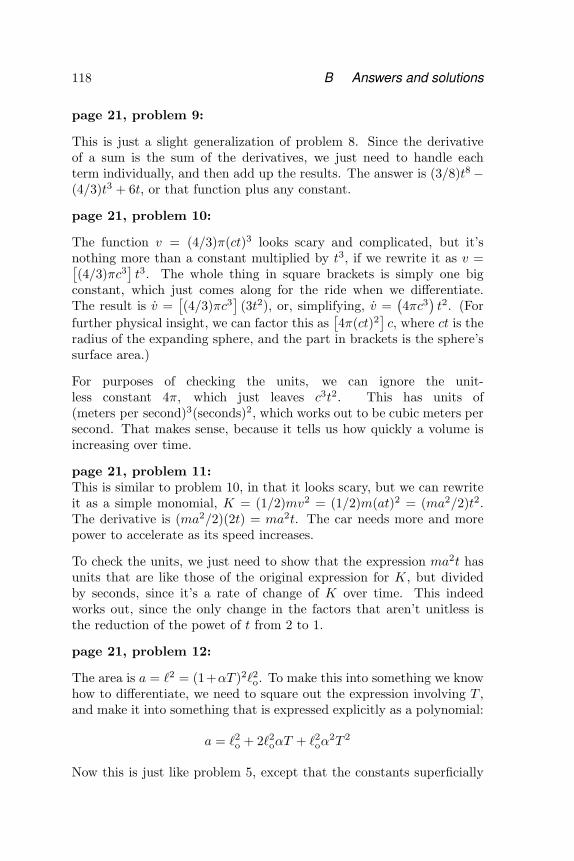
118 B Answers and solutions
page 21, problem 9:
This is just a slight generalization of problem 8. Since the derivativeof a sum is the sum of the derivatives, we just need to handle eachterm individually, and then add up the results. The answer is (3/8)t8−(4/3)t3 + 6t, or that function plus any constant.
page 21, problem 10:
The function v = (4/3)π(ct)3 looks scary and complicated, but it’snothing more than a constant multiplied by t3, if we rewrite it as v =[(4/3)πc3
]t3. The whole thing in square brackets is simply one big
constant, which just comes along for the ride when we differentiate.The result is v =
[(4/3)πc3
](3t2), or, simplifying, v =
(4πc3
)t2. (For
further physical insight, we can factor this as[4π(ct)2
]c, where ct is the
radius of the expanding sphere, and the part in brackets is the sphere’ssurface area.)
For purposes of checking the units, we can ignore the unit-less constant 4π, which just leaves c3t2. This has units of(meters per second)3(seconds)2, which works out to be cubic meters persecond. That makes sense, because it tells us how quickly a volume isincreasing over time.
page 21, problem 11:This is similar to problem 10, in that it looks scary, but we can rewriteit as a simple monomial, K = (1/2)mv2 = (1/2)m(at)2 = (ma2/2)t2.The derivative is (ma2/2)(2t) = ma2t. The car needs more and morepower to accelerate as its speed increases.
To check the units, we just need to show that the expression ma2t hasunits that are like those of the original expression for K, but dividedby seconds, since it’s a rate of change of K over time. This indeedworks out, since the only change in the factors that aren’t unitless isthe reduction of the powet of t from 2 to 1.
page 21, problem 12:
The area is a = `2 = (1+αT )2`2o. To make this into something we knowhow to differentiate, we need to square out the expression involving T ,and make it into something that is expressed explicitly as a polynomial:
a = `2o + 2`2oαT + `2oα2T 2
Now this is just like problem 5, except that the constants superficially
119
look more complicated. The result is
a = 2`2oα+ 2`2oα2T
= 2`2o(α+ α2T
).
We expect the units of the result to be area per unit temperature, e.g.,degrees per square meter. This is a little tricky, because we have tofigure out what units are implied for the constant α. Since the questiontalks about 1 + αT , apparently the quantity αT is unitless. (The 1 isunitless, and you can’t add things that have different units.) Thereforethe units of α must be “per degree,” or inverse degrees. It wouldn’tmake sense to add α and α2T unless they had the same units (andyou can check for yourself that they do), so the whole thing inside theparentheses must have units of inverse degrees. Multiplying by the `2oin front, we have units of area per degree, which is what we expected.
page 22, problem 13:
The first derivative is 6t2 − 1. Going again, the answer is 12t.
page 22, problem 14:
The first derivative is 3t2+2t, and the second is 6t+2. Setting this equalto zero and solving for t, we find t = −1/3. Looking at the graph, itdoes look like the concavity is down for t < −1/3, and up for t > −1/3.
c / Problem 14.
page 22, problem 15:
I chose k = −1, and t = 1. In other words, I’m going to check the slopeof the function x = t−1 = 1/r at t = 1, and see whether it really equalsktk−1 = −1. Before even doing the graph, I note that the sign makes

120 B Answers and solutions
sense: the function 1/t is decreasing for t > 0, so its slope should indeedbe negative.
d / Problem 15.
The tangent line seems to connect the points (0,2) and (2,0), so its slopedoes indeed look like it’s −1.
The problem asked us to consider the logical meaning of the two pos-sible outcomes. If the slope had been significantly different from −1given the accuracy of our result, the conclusion would have been that itwas incorrect to extend the rule to negative values of k. Although ourexample did come out consistent with the rule, that doesn’t prove therule in general. An example can disprove a conjecture, but can’t proveit. Of course, if we tried lots and lots of examples, and they all worked,our confidence in the conjecture would be increased.
page 53, problem 27:
(a) The Weierstrass definition requires that if we’re given a particular ε,and we be able to find a δ so small that f(x) + g(x) differs from F +Gby at most ε for |x− a| < δ. But the Weierstrass definition also tells usthat given ε/2, we can find a δ such that f differs from F by at mostε/2, and likewise for g and G. The amount by which f + g differs fromF +G is then at most ε/2 + ε/2, which completes the proof.
(b) Let dx be infinitesimal. Then the definition of the limit in terms ofinfinitesimals says that the standard part of f(a + dx) differs at mostinfinitesimally from F , and likewise for g and G. This means that f + gdiffers from F + G by the sum of two infinitesimals, which is itself aninfinitesimal, and therefore the standard part of f+g evaluated at x+dxequals F +G, satisfying the definition.

121
page 22, problem 16:
A minimum would occur where the derivative was zero. First we rewritethe function in a form that we know how to differentiate:
E(r) = ka12r−12 − 2ka6r−6
We’re told to have faith that the derivative of tk is ktk−1 even for k < 0,so
0 = E
= −12ka12r−13 + 12ka6r−7
To simplify, we divide both sides by 12k. The left side was already zero,so it keeps being zero.
0 = −a12r−13 + a6r−7
a12r−13 = a6r−7
a12 = a6r6
a6 = r6
r = ±a
To check that this is a minimum, not a maximum or a point of inflection,one method is to construct a graph. The constants a and k are irrelevantto this issue. Changing a just rescales the horizontal r axis, and changingk does the same for the vertical E axis. That means we can arbitrarilyset a = 1 and k = 1, and construct the graph shown in the figure. Thepoints r = ±a are now simply r = ±1. From the graph, we can seethat they’re clearly minima. Physically, the minimum at r = −a canbe interpreted as the same physical configuration of the molecule, butwith the positions of the atoms reversed. It makes sense that r = −abehaves the same as r = a, since physically the behavior of the systemhas to be symmetric, regardless of whether we view it from in front orfrom behind.
The other method of checking that r = a is a minimum is to take thesecond derivative. As before, the values of a and k are irrelevant, andcan be set to 1. We then have
E = −12r−13 + 12r−7
E = 156r−14 − 84r−8 .

122 B Answers and solutions
e / Problem 16.
Plugging in r = ±1, we get a positive result, which confirms that theconcavity is upward.
page 22, problem 17: Since polynomials don’t have kinks or end-points in their graphs, the maxima and minima must be points wherethe derivative is zero. Differentiation bumps down all the powers of apolynomial by one, so the derivative of a third-order polynomial is asecond-order polynomial. A second-order polynomial can have at mosttwo real roots (values of t for which it equals zero), which are givenby the quadratic formula. (If the number inside the square root in thequadratic formula is zero or negative, there could be less than two realroots.) That means a third-order polynomial can have at most twomaxima or minima.
Solutions for chapter 1
page 50, problem 1:
dxdt
=(t+ dt)4 − t4
dt
=4t3 dt+ 6t2dt2 + 4t dt3 + dt4
dt= 4t3 + . . . ,
where . . . indicates infinitesimal terms. The derivative is the standardpart of this, which is 4t3.
page 50, problem 2:
123
dxdt
=cos(t+ dt)− cos t
dtThe identity cos(α+ β) = cosα cosβ − sinα sinβ then gives
dxdt
=cos t cos dt− sin t sin dt− cos t
dt.
The small-angle approximations cos dt ≈ 1 and sin dt ≈ dt result in
dxdt
=− sin t dt
dt= − sin t .
page 50, problem 3:
H√H + 1−
√H − 1
1000 .0321000, 000 0.00101000, 000, 000 0.00032
The result is getting smaller and smaller, so it seems reasonable to guessthat if H is infinite, the expression gives an infinitesimal result.
page 50, problem 4:
dx√
dx.1 .32.001 .032.00001 .0032
The square root is getting smaller, but is not getting smaller as fast asthe number itself. In proportion to the original number, the square rootis actually getting bigger. It looks like
√dx is infinitesimal, but it’s still
infinitely big compared to dx. This makes sense, because√
dx equalsdx1/2. we already knew that dx0, which equals 1, was infinitely bigcompared to dx1, which equals dx. In the hierarchy of infinitesimals,dx1/2 fits in between dx0 and dx1.
page 50, problem 5:Statements (a)-(d), and (f)-(g) are all valid for the hyperreals, becausethey meet the test of being directly translatable, without having tointerpret the meaning of things like particular subsets of the reals in thecontext of the hyperreals.
Statement (e), however, refers to the rational numbers, a particularsubset of the reals, that that means that it can’t be mindlessly translated

124 B Answers and solutions
into a statement about the hyperreals, unless we had figured out a wayto translate the set of rational numbers into some corresponding subsetof the hyperreal numbers like the hyperrationals! This is not the type ofstatement that the transfer principle deals with. The statement is nottrue if we try to change “real” to “hyperreal” while leaving “rational”alone; for example, it’s not true that there’s a rational number that liesbetween the hyperreal numbers 0 and 0 + dx, where dx is infinitesimal.
page 51, problem 8: This would be a horrible problem if we had toexpand this as a polynomial with 101 terms, as in chapter 1! But nowwe know the chain rule, so it’s easy. The derivative is[
100(2x+ 3)99]
[2] ,
where the first factor in brackets is the derivative of the function onthe outside, and the second one is the derivative of the “inside stuff.”Simplifying a little, the answer is 200(2x+ 3)99.
page 51, problem 9:Applying the product rule, we get
(x+ 1)99(x+ 2)200 + (x+ 1)100(x+ 2)199 .
(The chain rule was also required, but in a trivial way — for both ofthe factors, the derivative of the “inside stuff” was one.)
page 51, problem 10:The derivative of e7x is e7x · 7, where the first factor is the derivative ofthe outside stuff (the derivative of a base-e exponential is just the samething), and the second factor is the derivative of the inside stuff. Thiswould normally be written as 7e7x.
The derivative of the second function is eex
ex, with the second expo-nential factor coming from the chain rule.
page 51, problem 11:We need to put together three different ideas here: (1) When a functionto be differentiated is multiplied by a constant, the constant just comesalong for the ride. (2) The derivative of the sine is the cosine. (3) Weneed to use the chain rule. The result is −ab cos(bx+ c).
page 51, problem 12:If we just wanted to fine the integral of sinx, the answer would be − cosx(or − cosx plus an arbitrary constant), since the derivative would be−(− sinx), which would take us back to the original function. Theobvious thing to guess for the integral of a sin(bx + c) would therefore
125
be −a cos(bx+ c), which almost works, but not quite. The derivative ofthis function would be ab sin(bx+ c), with the pesky factor of b comingfrom the chain rule. Therefore what we really wanted was the function−(a/b) cos(bx+ c).
page 51, problem 13:To find a maximum, we take the derivative and set it equal to zero. Thewhole factor of 2v2/g in front is just one big constant, so it comes alongfor the ride. To differentiate the factor of sin θ cos θ, we need to usethe chain rule, plus the fact that the derivative of sin is cos, and thederivative of cos is − sin.
0 =2v2
g(cos θ cos θ + sin θ(− sin θ))
0 = cos2 θ − sin2 θ
cos θ = ± sin θ
We’re interested in angles between, 0 and 90 degrees, for which boththe sine and the cosine are positive, so
cos θ = sin θtan θ = 1
θ = 45 ◦ .
To check that this is really a maximum, not a minimum or an inflectionpoint, we could resort to the second derivative test, but we know thegraph of R(θ) is zero at θ = 0 and θ = 90 ◦, and positive in between, sothis must be a maximum.
page 51, problem 14:Taking the derivative and setting it equal to zero, we have(ex − e−x) /2 = 0, so ex = e−x, which occurs only at x = 0. Thesecond derivative is (ex + e−x) /2 (the same as the original function),which is positive for all x, so the function is everywhere concave up, andthis is a minimum.
page 51, problem 15:(a) As suggested, let c =
√g/A, so that d = A ln cosh ct =
A ln (ect + e−ct). Applying the chain rule, the velocity is
Acect − ce−ct
cosh ct.
(b) The expression can be rewritten as Ac tanh ct.(c) For large t, the e−ct terms become negligible, so the velocity is

126 B Answers and solutions
Acect/ect = Ac. (d) From the original expression, A must have units ofdistance, since the logarithm is unitless. Also, since ct occurs inside afunction, ct must be unitless, which means that c has units of inversetime. The answers to parts b and c get their units from the factors ofAc, which have units of distance multiplied by inverse time, or velocity.
page 52, problem 16:Since I’ve advocated not memorizing the quotient rule, I’ll do this onefrom first principles, using the product rule.
ddθ
tan θ
=ddθ
(sin θcos θ
)=
ddθ
[sin θ (cos θ)−1
]= cos θ (cos θ)−1 + (sin θ)(−1)(cos θ)−2(− sin θ)
= 1 + tan2 θ
(Using a trig identity, this can also be rewritten as sec2 θ.)
page 52, problem 17:Reexpressing 3
√x as x1/3, the derivative is (1/3)x−2/3.
page 52, problem 18:(a) Using the chain rule, the derivative of (x2 + 1)1/2 is (1/2)(x2 +1)−1/2(2x) = x(x2 + 1)−1/2.(b) This is the same as a, except that the 1 is replaced with an a2, sothe answer is x(x2 + a2)−1/2. The idea would be that a has the sameunits as x.(c) This can be rewritten as (a+x)−1/2, giving a derivative of (−1/2)(a+x)−3/2.(d) This is similar to c, but we pick up a factor of −2x from the chainrule, making the result ax(a− x2)−3/2.
page 52, problem 19:By the chain rule, the result is 2/(2t+ 1).

127
page 52, problem 20:Using the product rule, we have(
ddx
3)
sinx+ 3(
ddx
sinx)
,
but the derivative of a constant is zero, so the first term goes away, andwe get 3 cosx, which is what we would have had just from the usualmethod of treating multiplicative constants.
page 52, problem 21:
N(Gamma(2))1
N(Gamma(2.00001))1.0000042278
N( (1.0000042278-1)/(.00001) )0.4227799998
Probably only the first few digits of this are reliable.
page 52, problem 22:The area and volume are
A = 2πr`+ 2πr2
and
V = πr2` .
The strategy is to use the equation for A, which is a constant, to elimi-nate the variable `, and then maximize V in terms of r.
` = (A− 2πr2)/2πr
Substituting this expression for ` back into the equation for V ,
V =12rA− πr3 .
128 B Answers and solutions
To maximize this with respect to r, we take the derivative and set itequal to zero.
0 =12A− 3πr2
A = 6πr2
` = (6πr2 − 2πr2)/2πr` = 2r
In other words, the length should be the same as the diameter.
page 52, problem 23:(a) We can break the expression down into three factors: the constantm/2 in front, the nonrelativistic velocity dependence v2, and the rela-tivistic correction factor (1 − v2/c2)−1/2. Rather than substituting inat for v, it’s a little less messy to calculate dK/dt = (dK/dv)(dv/dt) =adK/dv. Using the product rule, we have
dKdt
= a · 12m
[2v(
1− v2
c2
)−1/2
+v2 ·(− 1
2
) (1− v2
c2
)−3/2 (− 2vc2
)]= ma2t
[(1− v2
c2
)−1/2
+v2
2c2(
1− v2
c2
)−3/2]
(b) The expression ma2t is the nonrelativistic (classical) result, and hasthe correct units of kinetic energy divided by time. The factor in squarebrackets is the relativistic correction, which is unitless.(c) As v gets closer and closer to c, the expression 1− v2/c2 approacheszero, so both the terms in the relativistic correction blow up to positiveinfinity.
page 53, problem 24:We already know it works for positive x, so we only need to check itfor negative x. For negative values of x, the chain rule tells us that thederivative is 1/|x|, multiplied by −1, since d|x|/dx = −1. This gives−1/|x|, which is the same as 1/x, since x is assumed negative.
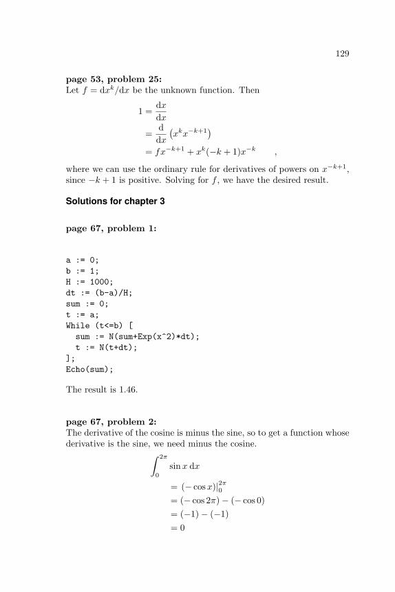
129
page 53, problem 25:Let f = dxk/dx be the unknown function. Then
1 =dxdx
=d
dx(xkx−k+1
)= fx−k+1 + xk(−k + 1)x−k ,
where we can use the ordinary rule for derivatives of powers on x−k+1,since −k + 1 is positive. Solving for f , we have the desired result.
Solutions for chapter 3
page 67, problem 1:
a := 0;b := 1;H := 1000;dt := (b-a)/H;sum := 0;t := a;While (t<=b) [sum := N(sum+Exp(x^2)*dt);t := N(t+dt);
];Echo(sum);
The result is 1.46.
page 67, problem 2:The derivative of the cosine is minus the sine, so to get a function whosederivative is the sine, we need minus the cosine.∫ 2π
0
sinx dx
= (− cosx)|2π0= (− cos 2π)− (− cos 0)= (−1)− (−1)= 0

130 B Answers and solutions
f / Problem 2.
As shown in figure f, the graph has equal amounts of area above andbelow the x axis. The area below the axis counts as negative area, sothe total is zero.
page 67, problem 3:
g / Problem 3.
The rectangular area of the graph is 2, and the area under the curvefills a little more than half of that, so let’s guess 1.4.
∫ 2
0
−x2 + 2x =(−1
3x3 + x2
)∣∣∣∣20
= (−8/3 + 4)− (0)= 4/3
This is roughly what we were expecting from our visual estimate.
131
page 67, problem 4:Over this interval, the value of the sin function varies from 0 to 1, andit spends more time above 1/2 than below it, so we expect the averageto be somewhat greater than 1/2. The exact result is
sin =1
π − 0
∫ π
0
sinx dx
=1π
(− cosx)|π0
=1π
[− cosπ − (− cos 0)]
=2π
,
which is, as expected, somewhat more than 1/2.
page 67, problem 5:Consider a function y(x) defined on the interval from x = 0 to 2 likethis:
y(x) =
{−1 if 0 ≤ x ≤ 11 if 1 < x ≤ 2
The mean value of y is zero, but y never equals zero.
page 67, problem 6:Let x be defined as
x(t) =
{0 if t < 01 if t ≥ 0
Integrating this function up to t gives
x(t) =
{0 if t ≤ 0t if t ≥ 0
The derivative of x at t = 0 is undefined, and therefore integrationfollowed by differentiation doesn’t recover the original function x.

132 B Answers and solutions
C Photo CreditsExcept as specifically noted below or in a parenthetical credit in the caption of afigure, all the illustrations in this book are under my own copyright, and are copyleftlicensed under the same license as the rest of the book.
In some cases it’s clear from the date that the figure is public domain, but I don’tknow the name of the artist or photographer; I would be grateful to anyone whocould help me to give proper credit. I have assumed that images that come fromU.S. government web pages are copyright-free, since products of federal agencies fallinto the public domain. I’ve included some public-domain paintings; photographicreproductions of them are not copyrightable in the U.S. (Bridgeman Art Library,Ltd. v. Corel Corp., 36 F. Supp. 2d 191, S.D.N.Y. 1999).
cover: Daniel Schwen, 2004; GFDL licensed 10 Gauss: C.A. Jensen (1792-1870).12 Newton: Godfrey Kneller, 1702. 23 Leibniz: Bernhard Christoph Francke,1700. 26 Berkeley: public domain?. 27 Robinson: source: www-groups.dcs.st-and.ac.uk, copyright status unknown. 88 Euler: Emanuel Handmann, 1753. 99tightrope walker: public domain, since Blondin died in 1897.
133

134 C Photo Credits
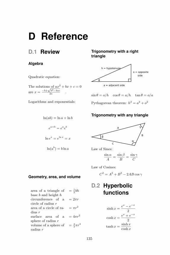
D ReferenceD.1 Review
Algebra
Quadratic equation:
The solutions of ax2 + bx+ c = 0
are x =−b±√
b2−4ac
2a.
Logarithms and exponentials:
ln(ab) = ln a+ ln b
ea+b = eaeb
ln ex = eln x = x
ln(ab) = b ln a
Geometry, area, and volume
area of a triangle ofbase b and height h
= 12bh
circumference of acircle of radius r
= 2πr
area of a circle of ra-dius r
= πr2
surface area of asphere of radius r
= 4πr2
volume of a sphere ofradius r
= 43πr3
Trigonometry with a righttriangle
sin θ = o/h cos θ = a/h tan θ = o/a
Pythagorean theorem: h2 = a2 + o2
Trigonometry with any triangle
Law of Sines:
sinα
A=
sinβ
B=
sin γ
C
Law of Cosines:
C2 = A2 +B2 − 2AB cos γ
D.2 Hyperbolicfunctions
sinhx =ex − e−x
2
coshx =ex + e−x
2
tanhx =sinhx
coshx
135
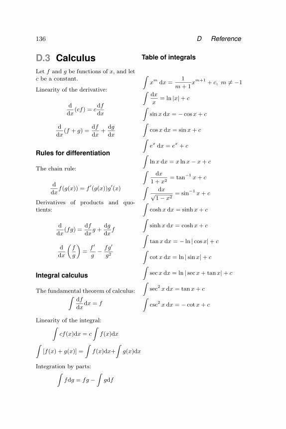
136 D Reference
D.3 CalculusLet f and g be functions of x, and letc be a constant.
Linearity of the derivative:
d
dx(cf) = c
df
dx
d
dx(f + g) =
df
dx+
dg
dx
Rules for differentiation
The chain rule:
d
dxf(g(x)) = f ′(g(x))g′(x)
Derivatives of products and quo-tients:
d
dx(fg) =
df
dxg +
dg
dxf
d
dx
„f
g
«=f ′
g− fg′
g2
Integral calculus
The fundamental theorem of calculus:Zdf
dxdx = f
Linearity of the integral:Zcf(x)dx = c
Zf(x)dxZ
[f(x) + g(x)] =
Zf(x)dx+
Zg(x)dx
Integration by parts:Zfdg = fg −
Zgdf
Table of integrals
Zxm dx =
1
m+ 1xm+1 + c, m 6= −1Z
dx
x= ln |x|+ cZ
sinx dx = − cosx+ cZcosx dx = sinx+ cZex dx = ex + cZlnx dx = x lnx− x+ cZ
dx
1 + x2= tan−1 x+ cZ
dx√1− x2
= sin−1 x+ cZcoshx dx = sinhx+ cZsinhx dx = coshx+ cZtanx dx = − ln | cosx|+ cZcotx dx = ln | sinx|+ cZsecx dx = ln | secx+ tanx|+ cZsec2 x dx = tanx+ cZcsc2 x dx = − cotx+ c

Indexarctangent, 76area
in Cartesian coordinates, 97in polar coordinates, 101
argument, 86average, 60
Berkeley, George, 26
calculusdifferential, 14fundamental theorem of
proof, 111statement, 58
integral, 14Cartesian coordinates, 101chain rule, 33complex number, 85
argument of, 86conjugate of, 86magnitude of, 86
concavity, 17conjugate, 86continuous function, 41coordinates
Cartesian, 101cylindrical, 102polar, 101spherical, 102
cosinederivative of, 25
cylindrical coordinates, 102
derivativechain rule, 33defined using a limit, 26, 41defined using infinitesimals, 29definition using tangent line, 14of a polynomial, 16, 107of a quotient, 37of a second-order polynomial, 15of square root, 33
of the cosine, 25of the exponential, 34, 110of the logarithm, 36of the sine, 25, 108product rule, 30properties of, 15second, 16undefined, 19
Descartes, Rene, 101differentiation
computer-aided, 38numerical, 40symbolic, 38
implicit, 70
Euler’s formula, 88Euler, Leonhard, 89exponential
definition of, 111derivative of, 34
factorial, 11, 73fission, 104fundamental theorem of algebra
proof, 112statement, 88
fundamental theorem of calculusproof, 111statement, 58
Galileo, 13Gauss, Carl Friedrich, 9
portrait, 9
halo, 29Holditch’s theorem, 68hyperbolic cosine, 51hyperbolic tangent, 52hyperinteger, 110hyperreal number, 27
imaginary number, 85
137

138 INDEX
implicit differentiation, 70improper integral, 93indeterminate form, 47infinitesimal number, 23
criticism of, 26safe use of, 26
infinity, 23inflection point, 18integral, 14
definitedefinition, 58
improper, 93indefinite
definition, 57iterated, 97properties of, 59
integrationcomputer-aided
numerical, 57symbolic, 39
methods ofby parts, 78change of variable, 76partial fractions, 79, 90
intermediate value theorem, 41iterated integral, 97
Kepler, Johannes, 69
L’Hopital’s rule, 45Leibniz notation
derivative, 24infinitesimal, 24integral, 57
Leibniz, Gottfried, 23limit, 26
definitioninfinitesimals, 42Weierstrass, 42
liquid drop model, 104logarithm
definition of, 36
magnitude of a complex number, 86maximum of a function, 18mean value theorem
proof, 112statement, 60
minimum of a function, 18moment of inertia, 99
Newton’s method, 69Newton, Isaac, 12normalization, 61nucleus, 104
partial fractions, 79, 90planets, motion of, 69polar coordinates, 101probability, 61product rule, 30
quotientderivative of, 37
radius of convergence, 74Robinson, Abraham, 27
sinederivative of, 25
spherical coordinates, 102standard deviation, 65standard part, 29
tangent lineformal definition, 107informal definition, 13
Taylor series, 71transfer principle, 27
applied to functions, 110
volumein cylindrical coordinates, 102in spherical coordinates, 103
work, 61