POLI 270 - Mathematical and Statistical FoundationsProf. S. SaieghFall 2010

Lecture Notes - Class 5

October 21, 2010

Calculus of Several Variables

So far in our study of calculus we have confined our attention to functions having a singleindependent variable.

We did this to keep things simple while we looked into such notions as graph of afunction, derivative, and so on.

However, most problems in the social sciences involve more than one independentvariable.

For example, if we want to study the relationship between political institutions and economicgrowth we might have to consider a large number of independent variables to obtain a realisticmodel.

Therefore, we must come to grips with the way functions of several variables are handledin calculus.

Functions of Two Variables

Here are some examples of functions of two variables x and y. For each choice of x, y, thereis a rule for computing the value of the function f(x, y).

f(x, y) = xy − x2

f(x, y) =√x2 + y2

f(x, y) = 12xy + 3x− 5y + 30

f(x, y) = 3

Function of Two Variables. A function f of two variables x and y is a rule thatassigns to each ordered pair (x, y) of real numbers in some set one and only onereal number denoted by f(x, y).

1

Consider the function f : R2 → R1 defined by f(x, y) = 4 + xy − x2.

As in the case of functions of one variable, we can find the value of f when x = 1 andy = 3,

f(1, 3) = 4 + (1)(3)− (1)2 = 6.

Similarly,

f(1, 0) = 4 + (1)(0)− (1)2 = 3.

More generally, the domain of a function of two variables f(x, y), is the set of all orderedpairs (x, y) of real numbers for which f(x, y) can be evaluated.

Example 1 Let f(x, y) = 3x2+5yx−y

.

Since division by any real number except zero is possible, the only ordered pairs (x, y)for which f cannot be evaluated are those for which x = y. Hence, the domain of f consistsof all ordered pairs (x, y) of real numbers for which x 6= y.

Visualizing Functions of Several Variables: Graphs and Level Curves

As we already know, functions of one variable can be represented graphically as curves drawnon a two-dimensional coordinate system.

In the case of functions of two variables, the way to visualize them is to represent themgraphically as surfaces drawn on a three-dimensional coordinate system.

There is, unfortunately, no easy way to visualize functions of more than two variables;they must be handled algebraically, without the aid of accurate pictures.

Before sketching the graph of a function z = f(x, y) of two variables we must set up coordi-nates in three-dimensional space.

2

We do this by marking an origin O and drawing three perpendicular coordinate axesthrough it.

It is customary to identify the the two horizontal axes with the independent variablesx and y, and the vertical axis with the dependent variable z.

That is, the xy plane is taken as horizontal.

The z axis is perpendicular to the xy plane, and the upward direction is chosen to bethe positive z direction.

Each point P in space is then described by three coordinates (a, b, c). Starting from theorigin, we reach P = (a, b, c) by moving a units in the x direction, b units parallel to the ydirection, and then c units parallel to the z axis.

For example, to reach the point P = (1, 2, 4) we move +1 unit in the x direction, then+2 units parallel to the y axis, and finally +4 units (move upward) parallel to the z axis.

3

Similarly, P = (2,−1,−3) represents the point that is 3 units below the xy plane andthat lies directly under the point (x, y) = (2,−1).

The origin O has coordinates (0,0,0), and the xy plane consists of all points P = (x, y, z)such that z = 0.

Namely, it is the solution set of the simple equation z = 0.

We do not move at all in the z direction to reach points in this plane.

Similarly, we define the xz plane and the yz plane, which are determined by theequations y = 0 and x = 0, respectively.

If f(x, y) is a function of two variables, its graph is a surface in three-dimensional space,determined as follows.

First, we sketch a copy of the feasible set for f in the xy plane by identifying pairs(x, y) for which f is defined with points (x, y, 0) in the xy plane.

In the following figure, the feasible set for the function f is indicated by the shadedregion in the xy plane.

4

Over each point Q = (x, y, 0) in this region, we then find the point P = (x, y, z) lying adistance z = f(x, y) above Q (or below Q if z = f(x, y) is negative).

As Q varies within the feasible set, the points P = (x, y, z) with z = f(x, y) trace outa surface.

This surface is the graph of f.

Conversely, if we are given the graph of a function f, we may determine the value z = f(x, y)geometrically.

We simply locate the point Q = (x, y, 0) in the xy plane and measure the distance zwe must move up or down to reach the corresponding point P = (x, y, z) on the surface.

Level Curves

Another way to portray the behavior of f is to sketch its level curves.

These are the curves in the xy plane consisting of all points (x, y) where f(x, y) takeson a particular constant value, say f(x, y) = c.

For each choice of the constant c there is a different level curve, the solution set of theequation f(x, y) = c.

Example 2 Let f(x, y) = x2 + y2. The level curve f(x, y) = c has the equation x2 + y2 = c.If c = 0, this is the point (0, 0), and if c > 0, it is a circle of radius

√c. If c < 0, there are

no points that satisfy x2 + y2 = c.

5

Notice that the level curves we have just found correspond to cross sections perpendicularto the z axis. It turns out that these cross sections perpendicular to the x axis and the yaxis are parabolas. For this reason, the surface is shaped like a bowl.

Level curves appear in many different applications in economics and political science. Forinstance, in economics, if the output Q(x, y) of a production process is determined by twoinputs x and y (say, hours of labor and capital investment), then the level curve Q(x, y) = cis called the curve of constant product c or, more simply, an isoquant.

In the case of political science, consider the classical problem in budgeting, in which agroup of legislators must decide how to divide expenditures between “guns” and “butter”.

Possible allocations are described by two numbers: dollars spent on butter and dollarsspent on guns.

Namely, the “policy space” is two-dimensional, and this is the domain over whichpreferences are expressed.

In this example, each legislator who is considering a particular allocation betweenthese two goods is associated with a utility function u(b, g), which measures the totalsatisfaction (or utility) the legislator derives from spending b dollars on butter, and gdollars on guns.

Suppose our legislator has an ideal point y in the policy space (i.e. her utility functionreaches a maximum over this point).

Assume also that her preferences decline with “distance” from this ideal point.

We can represent a legislator’s preferences with the following graph.

6

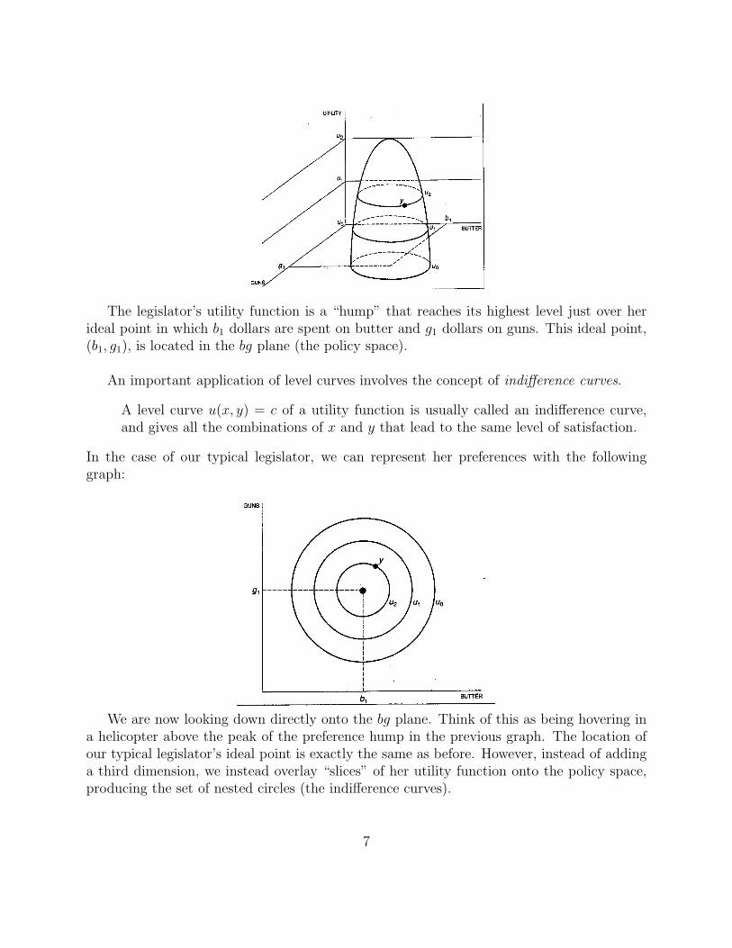
The legislator’s utility function is a “hump” that reaches its highest level just over herideal point in which b1 dollars are spent on butter and g1 dollars on guns. This ideal point,(b1, g1), is located in the bg plane (the policy space).

An important application of level curves involves the concept of indifference curves.

A level curve u(x, y) = c of a utility function is usually called an indifference curve,and gives all the combinations of x and y that lead to the same level of satisfaction.

In the case of our typical legislator, we can represent her preferences with the followinggraph:

We are now looking down directly onto the bg plane. Think of this as being hovering ina helicopter above the peak of the preference hump in the previous graph. The location ofour typical legislator’s ideal point is exactly the same as before. However, instead of addinga third dimension, we instead overlay “slices” of her utility function onto the policy space,producing the set of nested circles (the indifference curves).

7

Each circle is a slice of the policy hump in the three-dimensional graph. It is a locus ofpolicy outcomes among which the legislator is indifferent (since all the points on a circle lie onthe same slice and hence at the same height on the utility function of the three-dimensionalgraph).

Since we assumed that distance from an ideal point is a measure of preference, points ona circle centered on her ideal – being equidistant from that ideal,– are equally preferred byher. The logic is the same in comparing a point on one circle to that on another.

Our legislator, though, will prefer a point on a circle with a smaller radius to one on acircle with a larger radius, because this means the former point is closer to her ideal than isthe latter point.

Partial Derivatives

If f(x, y) is a function of two variables and P = (x, y) is a fixed base point in its feasible set,we may move in many directions to reach nearby points Q = (x+ ∆x, y + ∆y).

For example, if ∆x is arbitrary and ∆y = 0, we move horizontally, parallel to the xaxis, to reach the adjacent point Q ′ = (x+ ∆x, y).

If ∆y is arbitrary and ∆x = 0, then we move vertically from P to reach Q ′′ =(x, y + ∆y).

However, the increments ∆x and ∆y are independent of one another, and we may reach anypoint by choosing ∆x and ∆y appropriately.

For example, if P = (1, 1), and we wish to reach Q = (4,−1), we should take ∆x = 3and ∆y = −2 to get Q = (1 + ∆x, 1 + ∆y) = (4,−1).

As we can see, a “displacement” from one point P to another point Q is a quantitythat has both a magnitude and a direction.

8

Now let f(x, y) be any function defined at and near a point P = (x, y). The value of thefunction there is just f(P ) = f(x, y). At a nearby point Q = (x + ∆x, y + ∆y) its value isf(Q) = f(x+ ∆x, y + ∆y). Thus the change in the value of f is a real number

∆f = f(Q)− f(P ) = f(x+ ∆x, y + ∆y)− f(x, y)

but the change in the variable (the displacement from P to Q) is not a number. Thus, wecannot form averages as we did before when we considered functions of one variable.

We need a new idea to define rates of change and derivatives for functions of several variables.

The idea is this: If a base point P = (x, y) is given and we restrict attention todisplacements from P in the x direction only (∆x arbitrary, ∆y = 0), then the averagerate of change in the x direction

∆f

∆x=

f(x+ ∆x, y)− f(x, y)

∆x=

f(Q)− f(P )

∆x

is defined for all displacements ∆x 6= 0.

If these averages have a limit value as ∆x approaches zero, we obtain the rate of changeof f with respect to x (holding y fixed) at the point P .

This rate of change, if it exists, is denoted by

∂f

∂x(x, y) =

∂f

∂x(P ) = lim

∆x→0

( f(x+ ∆x, y)− f(x, y)

∆x

)and it is called the partial derivative of f with respect to x.

Similarly, we may define the partial derivative of f with respect to y as

∂f

∂y(x, y) =

∂f

∂y(P ) = lim

∆y→0

( f(x, y + ∆y)− f(x, y)

∆y

)by considering displacements from P parallel to the y axis.

A couple of remarks:

The partial derivatives ∂f∂x

and ∂f∂y

can have different values at different base points P .

They are usually defined whenever f is defined, so these partial derivatives are alsofunctions of two variables.

9

The question now is the following: how do we actually calculate partial derivatives?

Well, if we think of the limit values considered above in the right way, the problem ofcalculating ∂f

∂xand ∂f

∂yreduces to calculating ordinary derivatives of functions of one variable.

Thus, no new rules are needed for the computation of partial derivatives.

Computation of Partial Derivatives. To calculate ∂f∂x

simply regard y as aconstant whenever it appears in f(x, y), and differentiate the resulting functionof x in the ordinary way. The same rule, of course, applies to ∂f

∂y: Regard x as a

constant whenever it appears, and differentiate with respect to y.

The partial derivatives ∂f∂x

and ∂f∂y

can be denoted by any one of the following interchange-able symbols:

fx and fy ; Dxf and Dyf ; D1f and D2f .

Example 3 Let f(x, y) = 400 + x2 + y2 + 3xy.

Lets calculate ∂f∂x

(1, 3) and ∂f∂y

(1, 3) at the particular point P = (1, 3).

We find ∂f∂x

regarding y as a constant whenever it appears in the expression 400+x2+y2+3xy.Using standard rules for derivatives in one variable, we obtain

∂f

∂x= 2x+ 3y

Similarly, regarding x as a constant, we compute

∂f

∂y= 3x+ 2y

Setting x = 1 and y = 3 we obtain the values of the partial derivatives at the base pointP = (1, 3),

∂f

∂x(1, 3) = 2(1) + 3(3) = 11

∂f

∂y(1, 3) = 3(1) + 2(3) = 9

10

Note that the partial derivatives have other values at other base points. For example, atthe origin O = (0, 0) we obtain

∂f

∂x(0, 0) = 2(0) + 3(0) = 0

∂f

∂y(0, 0) = 3(0) + 2(0) = 0

If ∂f∂x

= 0 at a point (x, y), this means precisely that 2x+ 3y = 0, or y = −23x.

The solution set for the equation ∂f∂x

= 0 consists of all the points on the line determinedby 2x+ 3y = 0.

Notice that ∂f∂x

= 0 at infinitely many points in the plane.

Example 4 Let f(x, y) = 1000 + x2 + 3xy + 5y + 7y2.

Lets find now all points P = (x, y) where both partial derivatives are simultaneouslyequal to zero. Taking y as a constant everywhere it appears, we obtain

∂f

∂x= 2x+ 3y

Similarly, treating x as a constant, we obtain

∂f

∂y= 3x+ 5 + 14y.

The solution set for ∂f∂x

= 0 is the line given by 2x+ 3y = 0.

The equation ∂f∂y

= 0 gives a different line, determined by 3x+ 14y = −5.

The partial derivatives are both zero when P = (x, y) is a solution of the simultaneousequations

2x+ 3y = 0

3x+ 14y = −5

We have two equations with two unknowns, so we can solve them by substitution.

11

The first equation gives y = −23x. Substituting this into the second equation, we obtain

−5 = 3x+ 14(−2

3x)

−5 = −19

3x

x =15

19

Inserting x = 1519

into either equation, we find the corresponding value for y:

y = −2

3x

= −2

3

(15

19

)= −10

19

Thus P =(

1519,−10

19

)is the only point where ∂f

∂x= 0 and ∂f

∂y= 0 simultaneously.

Extrema and Critical Points of Functions of Two Variables

Given a function f(x, y) and a base point P , we say that:

(i) The function has a local maximum at P if f(P ) ≥ f(Q) for all points Q in the feasibleset lying near P .

(ii) The function has an absolute maximum at P if f(P ) ≥ f(Q) for all points Q in thefeasible set, whether they lie close to P or not.

Local (absolute) minima are defined similarly: f(P ) ≤ f(Q) for all nearby (all points) Qin the feasible set.

If either a maximum or a minimum occur at P , we may combine these possibilities bysaying that f has an extremum at P .

As in the case of functions of one variable, an absolute maximum (minimum) is also alocal maximum (minimum). However, the reverse need not be true.

A function may achieve its extreme values on the boundary of the feasible set (insofar asf is defined on this boundary) or at points interior to the feasible set.

12

An interior point P is one such that all points near P lie within the feasible set; the otherfeasible points are called boundary points.

This graph shows some possible locations of extrema.

There is an absolute minimum over point A on the boundary of the feasible set.

The absolute maximum is achieved at an interior point B.

In addition, there are local extrema that are not absolute extrema.

For example, the value of f at C is lower than all nearby values, but is not lower thanthe value at the corner point A; thus, a local minimum occurs at C.

The critical points of a function f(x, y) are those points P for which

∂f∂x

= 0 and ∂f∂y

= 0 simultaneously.

Like the critical points for functions of one variable, these critical points play an impor-tant role in the study of local extrema.

Suppose f(x, y) has a local maximum at over point P = (a, b). Then, the curve formedby intersecting the surface z = f(x, y) with the vertical plane y = b has a local maximumand hence a horizontal tangent when x = a.

13

Since the partial derivative ∂f∂x

(a, b) is the slope of this tangent, it follows that ∂f∂x

(a, b) = 0.

Similarly, the curve formed by intersecting the surface z = f(x, y) with the plane x = ahas a local maximum when y = b, and so ∂f

∂y(a, b) = 0.

This shows that a point at which a function of two variables has a local maximum mustbe a critical point. A similar argument shows that a point at which the function of twovariables has a local minimum must also be a critical point.

Extrema and Critical Points. An extremum for a function f(x, y) of two vari-ables can only occur

(i) at a critical point interior to the feasible set

or

(ii) at a boundary point of the feasible set.

In particular, every extremum interior to the feasible set reveals its presence bybeing a critical point.

14

All local extrema of a function must occur at critical points. However, not every criticalpoint of a function is necessarily a local extremum.

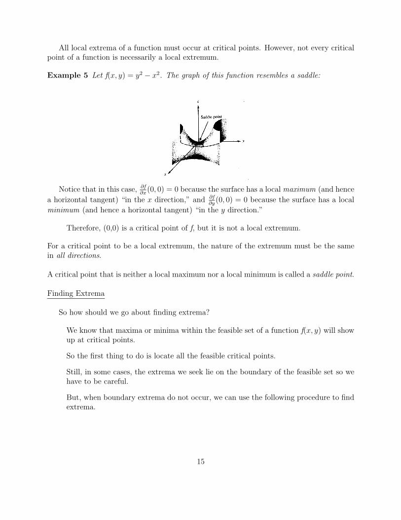
Example 5 Let f(x, y) = y2 − x2. The graph of this function resembles a saddle:

Notice that in this case, ∂f∂x

(0, 0) = 0 because the surface has a local maximum (and hence

a horizontal tangent) “in the x direction,” and ∂f∂y

(0, 0) = 0 because the surface has a local

minimum (and hence a horizontal tangent) “in the y direction.”

Therefore, (0,0) is a critical point of f, but it is not a local extremum.

For a critical point to be a local extremum, the nature of the extremum must be the samein all directions.

A critical point that is neither a local maximum nor a local minimum is called a saddle point.

Finding Extrema

So how should we go about finding extrema?

We know that maxima or minima within the feasible set of a function f(x, y) will showup at critical points.

So the first thing to do is locate all the feasible critical points.

Still, in some cases, the extrema we seek lie on the boundary of the feasible set so wehave to be careful.

But, when boundary extrema do not occur, we can use the following procedure to findextrema.

15

Finding Extrema. Suppose f(x, y) has an absolute maximum that does not occuron the boundary of the feasible set. It may be found as follows.

Step 1 Find the critical points P1, ...Pk within the feasible set by solving thesystem of equations

∂f∂x

= 0 ∂f∂y

= 0

These are the only candidates for solutions

Step 2 If there is just one candidate, the absolute maximum must occurthere. If there are several candidates P1, ...Pk then tabulate the valuesf(P1), ...f(Pk) of f at each of these points and compare. The largest value inthis list is the absolute maximum for f.

A similar procedure works for finding absolute minima.

Example 6 Let f(x, y) = 10 + x2 + 12y2 − x+ xy.

Let’s locate its absolute minimum and the absolute minimum value for f:

The feasible set consists of the whole coordinate plane, so there are no boundary points(or boundary extrema) to worry about.

We can find now all points P = (x, y) where both partial derivatives are simultaneouslyequal to zero.

∂f

∂x= 2x− 1 + y and

∂f

∂y= y + x.

Therefore, the simultaneous equations locating the critical points are

0 =∂f

∂x= 2x+ y − 1

0 =∂f

∂y= x+ y

This system has just one solution, the point P = (1,−1) where x = 1 and y = −1.

We have nothing to do in Step 2. The minimum is f(1,−1) = 9.5.

16

Higher-Order Partial Derivatives

If a function f(x, y) has partial derivatives ∂f∂x

and ∂f∂y

, we may apply the operations ∂∂x

and∂∂y

to each of these functions of two variables, thereby obtaining the second partial derivativesof f:

The partial derivative of fx with respect to x is

fxx = (fx)x or ∂2f∂x2 = ∂

∂x

(∂f∂x

)The partial derivative of fx with respect to y is

fxy = (fx)y or ∂2f∂y∂x = ∂

∂y

(∂f∂x

)The partial derivative of fy with respect to x is

fyx = (fy)x or ∂2f∂x∂y = ∂

∂x

(∂f∂y

)The partial derivative of fy with respect to y is

fyy = (fy)y or ∂2f∂y2 = ∂

∂y

(∂f∂y

)For all functions we are going to deal with, the “mixed” second partial derivatives agree:

∂2f∂y∂x = ∂2f

∂x∂y

Example 7 Let f(x, y) = 4x2 − 2xy + y3 + 10.

We are going to calculate the first and second partial derivatives of f, and the values ofthe second partial derivatives at the particular points P1 = (1, 3) and P2 = (−1, 0).

∂f

∂x= 8x− 2y

and

∂f

∂y= −2x+ 3y2.

Now we apply ∂∂x

and ∂∂y

to each of these functions to obtain the second partial derivatives:

17

∂

∂x(8x− 2y) = 8

∂

∂x(−2x+ 3y2) = −2

and

∂

∂y(8x− 2y) = −2

∂

∂y(−2x+ 3y2) = 6y

Notice that the mixed partials are equal, so we could have skipped one of the computa-tions.

At P1 = (1, 3) the values of the second partial derivatives are:

∂2f∂x2 (1, 3) = 8 ∂2f

∂x∂y(1, 3) = ∂2f∂y∂x(1, 3) = −2

∂2f∂y2 (1, 3) = 6(3) = 18

At P1 = (−1, 0) we have

∂2f∂x2 (−1, 0) = 8 ∂2f

∂x∂y(−1, 0) = ∂2f∂y∂x(−1, 0) = −2

∂2f∂y2 (−1, 0) = 6(0) = 0

Using the second derivative to find extrema

For a function f(x, y) of two variables, the first partial derivatives ∂f∂x

and ∂f∂y

taken to-

gether play the same role as the ordinary derivative dfdx

when f is a function of one variable.

Similarly, the whole set of second partial derivatives plays the role of d2fdx2 .

18

The second partial derivatives of f(x, y) are often presented in a little two-by-two arraycalled the Hessian matrix for f:

[∂2f∂x2

∂2f∂x∂y

∂2f∂y∂x

∂2f∂y2

]

Its determinant, called the discriminant of f is given by the following combination ofsecond partial derivatives

discriminant D(x, y) =(

∂2f∂x2

)(∂2f∂y2

)−(

∂2f∂x∂y

)2

and is another function of x and y. The discriminant will be used to test for maximaand minima when we come to optimization problems.

Example 8 Let f(x, y) = x3 − x+ y2 + xy.

In order to find the discriminant of f as a function of x and y, we first calculate the partialderivatives in the usual way

∂f

∂x= 3x2 − 1 + y

∂f

∂y= 2y + x

and

∂2f

∂x2= 6x

∂2f

∂x∂y=

∂2f

∂y∂x= 1

∂2f

∂y2= 2

19

By definition of the discriminant,

D(x, y) =( ∂2f

∂x2

)( ∂2f

∂y2

)−( ∂2f

∂x∂y

)2

= (6x)(2)− (1)2

= 12x− 1

Now we are finally ready to use a procedure involving second-order partial derivativesthat we can use to decide whether a given critical point is an extremum or a saddle point.

This procedure is the two-variable version of the second derivative test for functions of asingle variable that we covered in this course before.

The Second Derivative Test. Suppose P = (x0, y0) is a critical point for f(x, y), so that

∂f∂x

(P ) = 0 and ∂f∂y

(P ) = 0

To test P we form the discriminant

D(P ) = ∂2f∂x2 (P ) � ∂2f

∂y2 (P )−(

∂2f∂x∂y

(P ))2

out of the second partial derivatives. Then,

Step 1 If D(P ) < 0, the function does not have an extremum at P .

Step 2 If D(P ) > 0, and ∂2f∂x2 (P ) < 0, a local maximum occurs at P .

Step 3 If D(P ) > 0, and ∂2f∂x2 (P ) > 0, a local minimum occurs at P .

If D(P ) = 0, the test gives no information about P .

Example 9 Let f(x, y) = x2 + y2.

We are going to classify the critical point of this function using the second derivativetest. First, notice that

∂f∂x

= 2x and ∂f∂y

= 2y

so the only critical point of f is P = (0, 0). To test this point, we use the second-orderpartial derivatives

20

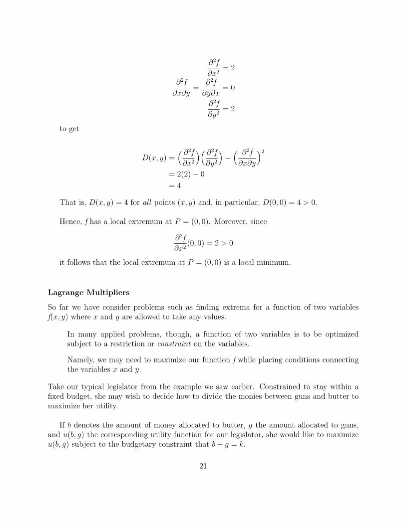
∂2f

∂x2= 2

∂2f

∂x∂y=

∂2f

∂y∂x= 0

∂2f

∂y2= 2

to get

D(x, y) =( ∂2f

∂x2

)( ∂2f

∂y2

)−( ∂2f

∂x∂y

)2

= 2(2)− 0

= 4

That is, D(x, y) = 4 for all points (x, y) and, in particular, D(0, 0) = 4 > 0.

Hence, f has a local extremum at P = (0, 0). Moreover, since

∂2f

∂x2(0, 0) = 2 > 0

it follows that the local extremum at P = (0, 0) is a local minimum.

Lagrange Multipliers

So far we have consider problems such as finding extrema for a function of two variablesf(x, y) where x and y are allowed to take any values.

In many applied problems, though, a function of two variables is to be optimizedsubject to a restriction or constraint on the variables.

Namely, we may need to maximize our function f while placing conditions connectingthe variables x and y.

Take our typical legislator from the example we saw earlier. Constrained to stay within afixed budget, she may wish to decide how to divide the monies between guns and butter tomaximize her utility.

If b denotes the amount of money allocated to butter, g the amount allocated to guns,and u(b, g) the corresponding utility function for our legislator, she would like to maximizeu(b, g) subject to the budgetary constraint that b+ g = k.

21

We can solve this problem using the method of Lagrange multipliers.

The Method of Lagrange Multipliers. Suppose f(x, y), and g(x, y) are functions whosefirst-order partial derivatives exist.

To find the local extrema of f(x, y) subject to the constraint that g(x, y) = k for some constantk, we introduce a new variable λ (the Greek letter lambda) and solve the following threeequations simultaneously

∂f

∂x= λ

∂g

∂x∂f

∂y= λ

∂g

∂y

g(x, y) = k

The desired local extrema will be found among the resulting points (x, y).

Example 10 Maximixe f(x, y) = xy subject to x2 + 4y2 = 1.

First, recall that we must solve the following three equations simultaneously,

∂f

∂x= λ

∂g

∂x∂f

∂y= λ

∂g

∂y

g(x, y) = k

Thus,

∂

∂x(f− g) = 0

∂

∂y(f− g) = 0

g(x, y) = x2 + 4y2 − 1 = 0

These conditions assert that the expression in x, y, λ,

l(x, y, λ) ≡ f(x, y)− λg(x, y)

known as the Lagrangian of the problem has a critical point. In this case,

l(x, y, λ) = xy − λ(x2 + 4y2 − 1).

22

Then

∂l

∂x= y − 2λx = 0 or λ =

y

2x∂l

∂y= x− 8λy = 0 or λ =

x

8y.

Multiplying together we obtain

λ2 =1

16or λ = ±1

4.

Hence

y = 2λx = ±1

2x.

Substituting into the constraint equation

x2 + 4(±1

2x)2

= 1

gives

2x2 = 1

or

x = ± 1√2

and

y = ± 1

2√

2.

Therefore, the function f(x, y) = xy is maximized at the points P1 = ( 1√2, 1

2√

2) and

P2 = (− 1√2,− 1

2√

2), where its value is 1

4.

It is minimized at the other two points, i.e. P3 = ( 1√2,− 1

2√

2) and P4 = (− 1√

2, 1

2√

2), where

the value of f is −14.

23

The Chain Rule

Suppose now that we have the composite function g(h1(x), h2(x), ·, ·.·, hn(x)). If h(x) hasonly one component, then we can use the Chain Rule (from week 2) to compute

ddx

g(h(x)) = g ′(h(x)) · h ′(x)

In words, the derivative of the composite function g(h(x)) is the derivative of the outsidefunction g(x) (evaluated at the inside function) times the derivative of the inside functionh(x).

Suppose now that the function under consideration has more than one inside function.In this case, we compute the derivative using an analogue of our last expression. We takethe derivative with respect to each inside function one at a time:

ddx = ∂g

∂h1(h(x))h′1(x) + ∂g

∂h2(h(x))h′2(x) + · · ·+ ∂g

∂hn(h(x))h′n(x)

The derivative of the composite function is the derivative ∂g∂h1

of g with respect to thefirst inside slot times the derivative of the function h1(x) in the first slot plus the derivative∂g∂h2

of g with respect to the second slot times the derivative of the function h2(x) of g in thatslot, and so on.

Example 11 Let f(x, y) = x2 + y2, x(t) = t, and y(t) = t.

The composite function g(t) = f(x(t), y(t)). Suppose that we want to compute the deriva-tive of g(t) when t = 1. If we use the Chain Rule, we first compute ∂f

∂x= 2x and ∂f

∂y= 2y,

and x′(t) = y′(t) = 1. When t = 1, x = y = 1. Therefore,

g′(1) = ∂f∂x (1, 1) · 1 + ∂f

∂y (1, 1) · 1 = 2 · 1 + 2 · 1 = 4

We can further check this result by computing the derivative of g in a more direct man-ner. Since g(t) = 2t2, g′(t) = 4t and g′(1) = 4.

24

Implicit Differentiation

The method of implicit differentiation is an outgrowth of the chain rule.

Often a function y = f(x) is described as the solution of an equation involving x andy, such as x2y + y = 1, or x3 − xy + y3 = 1.

Sometimes we can solve the equation, rearranging it by algebraic manipulations to get yon one side and a formula involving x on the other.

For example, we can solve the first expression to obtain y = 1x2+1

.

The second expression, though, is not so nice; no simple formula expresses y directly interms of x. Nonetheless, the original expression implicitly determines y as a function of xeven though finding the actual formula may be beyond our capabilities.

Using the chain rule, we may discuss the derivatives dydx

of such functions withoutsolving the equation that relates x and y.

The idea is to take the derivative ddx

of both sides of the expression.

In doing so, remember that y is regarded as a function of x (y = f(x)).

Thus an expression like y3 = y(x)3 –or more generally, yr = y(x)r where r is a realexponent – must be handled using the chain rule,

d

dx(yr) =

d

dx(y(x)r) = ry(x)r−1 · dy

dx= ryr−1 · dy

dx.

In this case, ddx

(y3) = 3y2 dydx

.

Going back to our problem, we take the derivative of the left hand side, and obtain:

d

dx(x3) = 3x2

d

dx(xy) = x · dy

dx+ y · d

dx= y + x

dy

dx

and

d

dx(y3) = 3y2 dy

dx.

Putting all these together, we find the derivative of the left hand side of the originalexpression

d

dx(x3 − xy + y3) = 3x2 − y − xdy

dx+ 3y2 dy

dx.

25

The derivative of the right hand side of the expression is ddx

(1) = 0. Comparing theresults, we get an equation

3x2 − y − xdydx

+ 3y2 dy

dx= 0

which can be solved for dydx

.

(3y2 − x)dy

dx= y − 3x2

or

dy

dx=y − 3x2

3y2 − x.

At x = 1, y = 0, we find

y′(1) =0− 3(1)2

3(0)2 − 1=−3

−1= 3.

Therefore, we can conclude that if there is a function y(x) which solves our original expres-sion and if it is differentiable, then as x changes by ∆x, the corresponding y will change by3∆x.

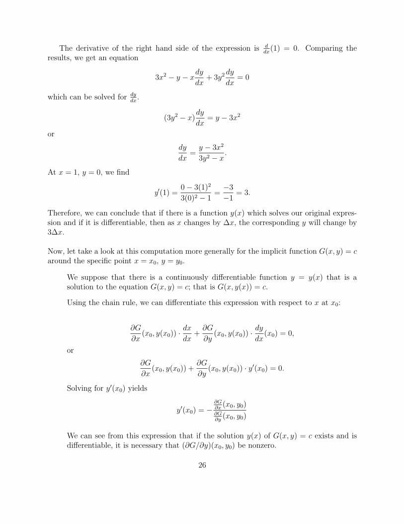
Now, let take a look at this computation more generally for the implicit function G(x, y) = caround the specific point x = x0, y = y0.

We suppose that there is a continuously differentiable function y = y(x) that is asolution to the equation G(x, y) = c; that is G(x, y(x)) = c.

Using the chain rule, we can differentiate this expression with respect to x at x0:

∂G

∂x(x0, y(x0)) · dx

dx+∂G

∂y(x0, y(x0)) · dy

dx(x0) = 0,

or

∂G

∂x(x0, y(x0)) +

∂G

∂y(x0, y(x0)) · y′(x0) = 0.

Solving for y′(x0) yields

y′(x0) = −∂G∂x

(x0, y0)∂G∂y

(x0, y0)

We can see from this expression that if the solution y(x) of G(x, y) = c exists and isdifferentiable, it is necessary that (∂G/∂y)(x0, y0) be nonzero.

26

Let’s go back to our example: x3 − xy + y3 = 1.

We can re-write this expression as G(x, y) ≡ x3 − xy + y3 − 1 = 0.

About the point (x0, y0) = (1, 0), one computes that

∂G

∂x= 3x2 − y = 3.

∂G

∂y= −x+ 2y2 = −1.

Since (∂G/∂y)(1, 0) = −1 6= 0, the expression does indeed define y as a continuouslydifferentiable function of x around x0 = 1, y0 = 0. Furthermore,

y′(1) = −∂G∂x

(1, 0)∂G∂y

(1, 0)= − 3

(−1)= 3.

just as we discovered before.

27