calculus the way to do it | free sample ebook | mathslearning.com | mathematics publishing company

© Mathematics Publishing Company – ‘Calculus … the way to do it’ Book 1. Available from www.mathslearning.com. Email: [email protected]

1


2

‘Calculus…the way to do it’ – Book 1

The Author:

R.M. O’Toole B.A., M.C., M.S.A., C.I.E.A.

The author is an experienced State Examiner, teacher, lecturer, consultant and author in mathematics.

She is an Affiliate Member of the Chartered Institute of Educational Assessors and a Member of The Society of Authors.

COPYRIGHT NOTICE

All rights reserved: no part of this work may be reproduced without either the prior written permission of the Publishers or a licence permitting restricted copying issued by the Copyright Licensing Agency, 90, Tottenham Road, London, WIP 9HE. This book may not be lent, resold, hired out or otherwise disposed of by way of trade in any form of binding or cover other than that in which it is published, without the prior consent of the Mathematics Publishing Company. © This publication has been deposited with ‘The Legal Deposit Office’, British Library, Boston Spa, Wetherby, W. Yorkshire, LS 23 7BY.

ISBN No. 978-1-900043-36-6

First Published in 1996 (Revised in 2015) by:

Mathematics Publishing Company, ‘The Cottage’ 45, Blackstaff Road, Clough, Downpatrick, Co. Down, BT30 8SR.

Tel. 028 44 851818 Fax. 028 44 851818

Email [email protected]


3

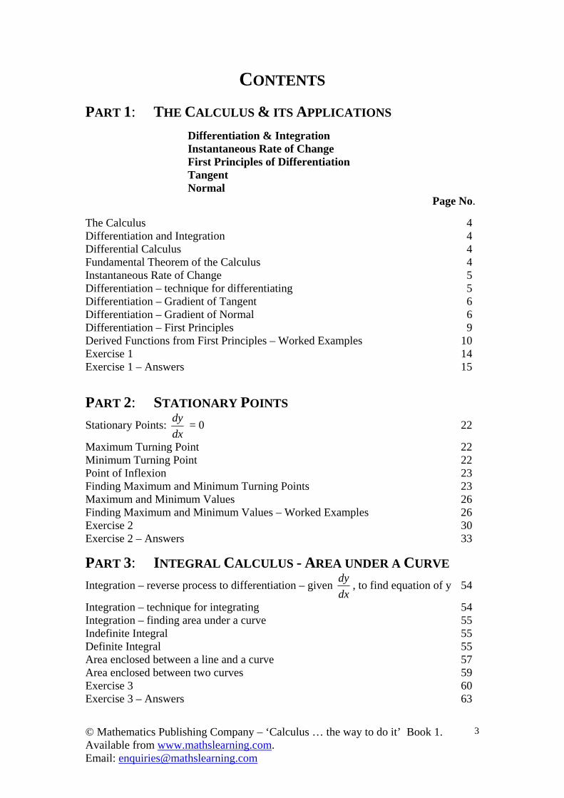
CONTENTS

PART 1: THE CALCULUS & ITS APPLICATIONS

Differentiation & Integration Instantaneous Rate of Change First Principles of Differentiation Tangent Normal

Page No.

The Calculus 4 Differentiation and Integration 4 Differential Calculus 4 Fundamental Theorem of the Calculus 4 Instantaneous Rate of Change 5 Differentiation – technique for differentiating 5 Differentiation – Gradient of Tangent 6 Differentiation – Gradient of Normal 6 Differentiation – First Principles 9 Derived Functions from First Principles – Worked Examples 10 Exercise 1 14 Exercise 1 – Answers 15

PART 2: STATIONARY POINTS

Stationary Points: dx

dy = 0 22

Maximum Turning Point 22 Minimum Turning Point 22 Point of Inflexion 23 Finding Maximum and Minimum Turning Points 23 Maximum and Minimum Values 26 Finding Maximum and Minimum Values – Worked Examples 26 Exercise 2 30 Exercise 2 – Answers 33

PART 3: INTEGRAL CALCULUS - AREA UNDER A CURVE

Integration – reverse process to differentiation – given dx

dy, to find equation of y 54

Integration – technique for integrating 54 Integration – finding area under a curve 55 Indefinite Integral 55 Definite Integral 55 Area enclosed between a line and a curve 57 Area enclosed between two curves 59 Exercise 3 60 Exercise 3 – Answers 63


4

PART 1

THE CALCULUS & ITS APPLICATIONS

PART 1 -DIFFERENTIATION & INTEGRATION INSTANTANEOUS RATE OF CHANGE

FIRST PRINCIPLES OF DIFFERENTIATION TANGENT NORMAL

The Calculus is one of the most useful disciplines in mathematics. It deals with changing quantities.

The Calculus has two main branches:

(i) Differential Calculus

(ii) Integral Calculus.

The central problem of differential calculus is to find the rate at which a known, but varying quantity, changes.

Integral calculus has the reverse problem. It tries to find a quantity when its rate of change is known.

There is, therefore, an inverse relationship between differentiation and integration. This inverse relationship is ‘The Fundamental Theorem of the Calculus’; it means that one process undoes the other, as, for example, addition of 2 undoes subtraction of 2, subtraction of 5 undoes addition of 5, multiplication by 3 undoes division by 3 or multiplication by 7 undoes division by 7.

(i) DIFFERENTIAL CALCULUS

The calculus deals with functions. A function f is a correspondence that associates with each number x some number f(x).

Eg. The formula, y = 2x 2 associates with each number x some number y. If we use f to label this function, then f(x) = 2x 2 .

Thus f(0) = 0, f(1) = 2, f(2) = 8, f(-1) = 2 and so on.


5

INSTANTANEOUS RATE OF CHANGE

The instantaneous rate of change of a function is so important that mathematics has given it a special name, derivative, i.e. the derived function.

There are different notations used for the derivative of a function; it depends on the notation used to represent the function itself:

Eg. If f(x) = 2x 2 , the derivative of f is denoted by f(x) and for y = 2x 2 (letting y = f(x)), the derivative of y

is denoted by dx

dy .

Remember, dx

dy is just notation to represent the derivative

of y with respect to x:

If s = 2t 2 , the derivative using this Leibnizian

notation is dt

ds , representing the rate of change of

s with t. (Baron von Leibniz (1646 – 1716), a German scholar, mathematician and philosopher, shares with Sir Isaac Newton the distinction of developing the theory of the differential and integral calculus, but his notation was adopted, in favour of Newton’s.)

The technique for differentiating a function is as follows:

(1) Premultiply by index. (2) Subtract 1 from index to give new index. (3) The derivative of a constant is 0. (4) Coefficients are not affected by differentiation.

Eg. 1 y = 2x 3 - 2x3

2 + x – 3

dx

dy = 6x 2 - 3

4 x + 1.

Eg. 2 f(x) = x 3 - 3

1 x 2 - 2

1 x + 5

f(x) = 3x 2 - 3

2 x - 2

1 .


6

Differentiating a function is equivalent to finding the gradient of the curve. The gradient of a curve at any point is the same as the gradient of the tangent to the curve at that point. Doing this ‘manually’ by drawing the tangent to the curve at the point and calculating its gradient is neither convenient nor accurate. Since differentiation is both convenient and accurate, it is certainly the preferred method for finding the gradient of a curve. However, being able to perform the operations graphically is fundamental to one’s understanding of the processes involved in the calculus, and it also demonstrates what a powerful tool the calculus is; it is so much quicker, (no need even to draw a graph), and its findings are 100% accurate.

dx

dy (or f(x), if you prefer), then, gives a general expression for

the gradient of a curve at any point on the curve. All that is required to find the actual gradient at a particular point is to substitute the value of x at that point into the general expression

for the gradient, i.e. the derivative, dx

dy .

Eg. 1.

If y = 2x 2 + x – 1, find the gradient of the curve at the point where x = 1, and, hence, find the equation of the tangent to the curve at the point (1, 2).

y = 2x 2 + x – 1

dx

dy = 4x + 1

x = 1 dx

dy = 4(1) + 1 = 5.

the gradient of the curve at the point where x = 1 is 5. the gradient of the tangent is also 5, we have:

y = mx + c (Remember the tangent is a straight line.) (1, 2) and m = 5 2 = 5(1) + c

2 = 5 + c -3 = c.

y = 5x – 3 is the equation of the tangent to the curve,

y = 2x 2 + x – 1, at the point (1, 2).


7

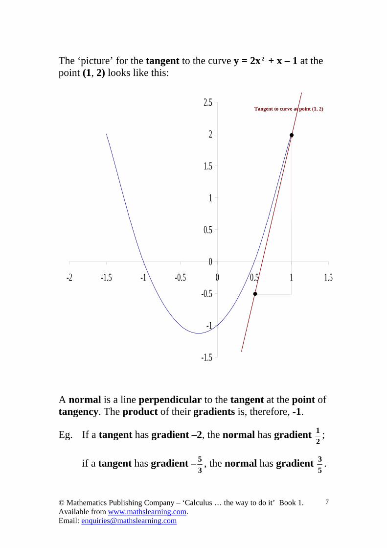
The ‘picture’ for the tangent to the curve y = 2x 2 + x – 1 at the point (1, 2) looks like this:

-1.5

-1

-0.5

0

0.5

1

1.5

2

2.5

-2 -1.5 -1 -0.5 0 0.5 1 1.5

A normal is a line perpendicular to the tangent at the point of tangency. The product of their gradients is, therefore, -1.

Eg. If a tangent has gradient –2, the normal has gradient 2

1 ;

if a tangent has gradient –3

5 , the normal has gradient 5

3 .

Tangent to curve at point (1, 2)


8

Eg. 2.

Find the equation of the normal to the curve, y = 2x 2 + x – 1 at the point (1, 2).

the tangent has gradient 5, (already found)

the normal has gradient -5

1.

Then y = mx + c gives:

2 = -5

1 (1) + c

c = 5

11 .

y = -5

1 x + 5

11 or 5y = 11 – x is the equation of the

normal to the curve, y = 2x 2 + x – 1, at the point (1, 2).

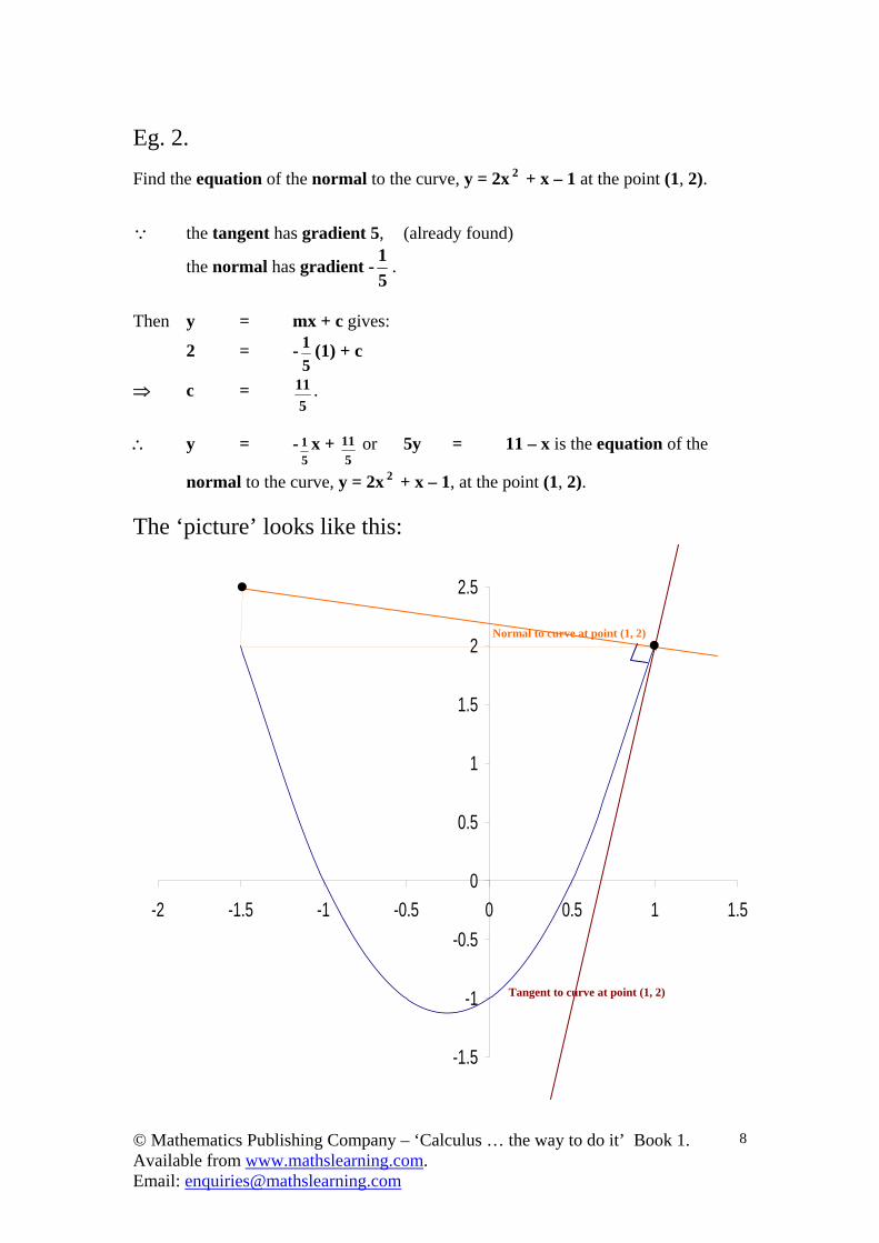
The ‘picture’ looks like this:

-1.5

-1

-0.5

0

0.5

1

1.5

2

2.5

-2 -1.5 -1 -0.5 0 0.5 1 1.5

Normal to curve at point (1, 2)

Tangent to curve at point (1, 2)


9

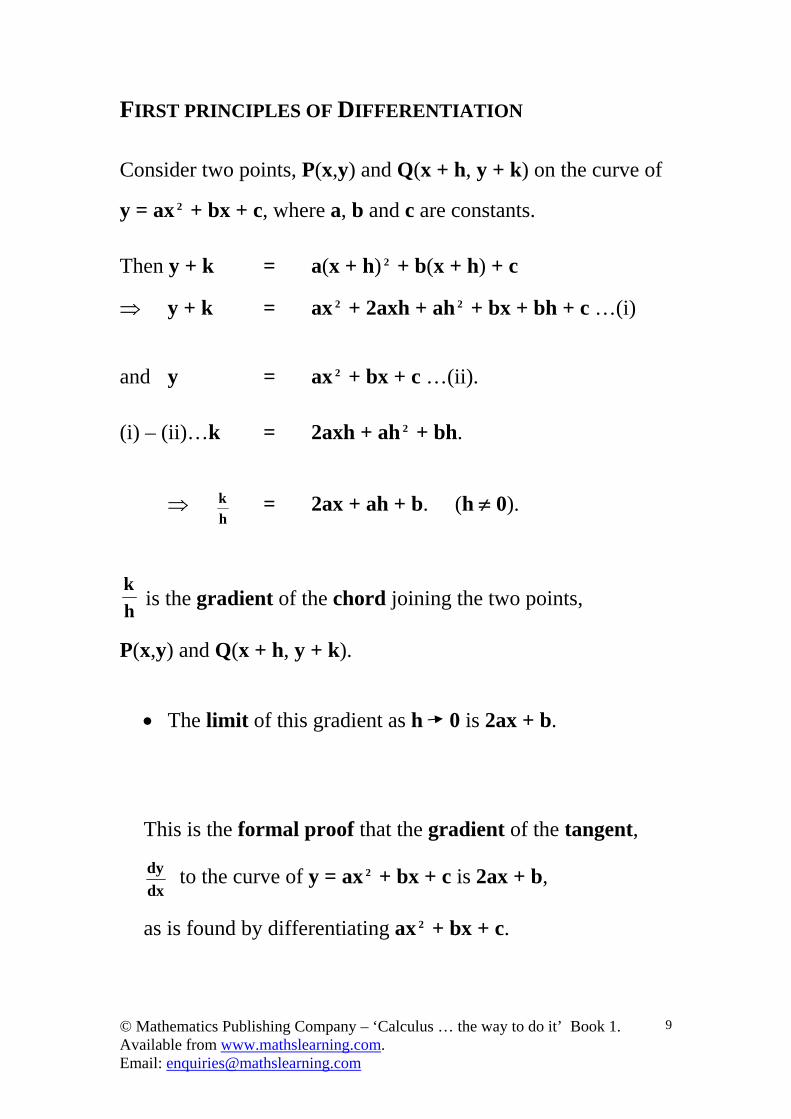
FIRST PRINCIPLES OF DIFFERENTIATION

Consider two points, P(x,y) and Q(x + h, y + k) on the curve of

y = ax 2 + bx + c, where a, b and c are constants.

Then y + k = a(x + h) 2 + b(x + h) + c

y + k = ax 2 + 2axh + ah 2 + bx + bh + c …(i)

and y = ax 2 + bx + c …(ii).

(i) – (ii)…k = 2axh + ah 2 + bh.

h

k = 2ax + ah + b. (h 0).

h

k is the gradient of the chord joining the two points,

P(x,y) and Q(x + h, y + k).

The limit of this gradient as h 0 is 2ax + b.

This is the formal proof that the gradient of the tangent,

dx

dy to the curve of y = ax 2 + bx + c is 2ax + b,

as is found by differentiating ax 2 + bx + c.


10

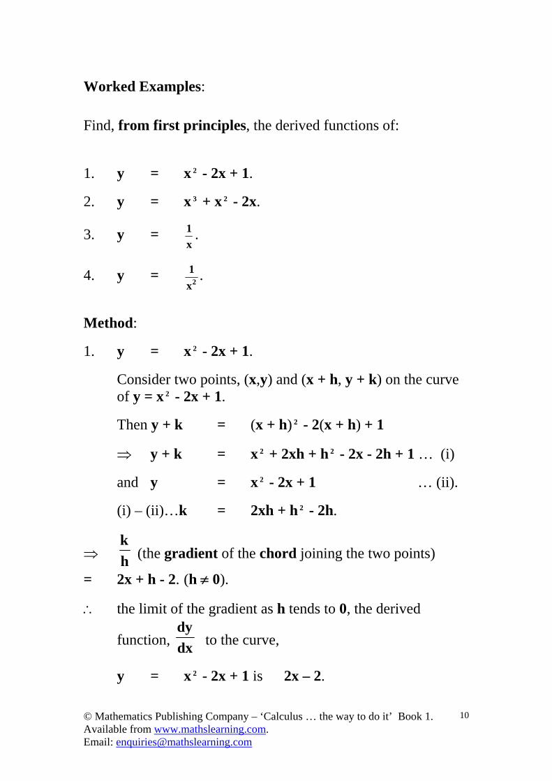
Worked Examples:

Find, from first principles, the derived functions of:

1. y = x 2 - 2x + 1.

2. y = x 3 + x 2 - 2x.

3. y = x

1 .

4. y = 2x

1 .

Method:

1. y = x 2 - 2x + 1.

Consider two points, (x,y) and (x + h, y + k) on the curve of y = x 2 - 2x + 1.

Then y + k = (x + h) 2 - 2(x + h) + 1

y + k = x 2 + 2xh + h 2 - 2x - 2h + 1 … (i)

and y = x 2 - 2x + 1 … (ii).

(i) – (ii)…k = 2xh + h 2 - 2h.

h

k (the gradient of the chord joining the two points)

= 2x + h - 2. (h 0).

the limit of the gradient as h tends to 0, the derived

function, dx

dy to the curve,

y = x 2 - 2x + 1 is 2x – 2.


11

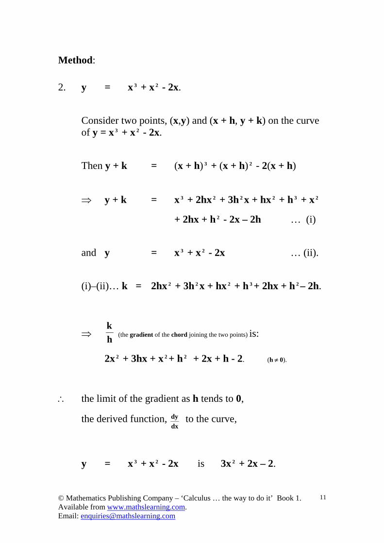
Method:

2. y = x 3 + x 2 - 2x.

Consider two points, (x,y) and (x + h, y + k) on the curve of y = x 3 + x 2 - 2x.

Then y + k = (x + h) 3 + (x + h) 2 - 2(x + h)

y + k = x 3 + 2hx 2 + 3h 2 x + hx 2 + h 3 + x 2

+ 2hx + h 2 - 2x – 2h … (i)

and y = x 3 + x 2 - 2x … (ii).

(i)–(ii)… k = 2hx 2 + 3h 2 x + hx 2 + h 3 + 2hx + h 2 – 2h.

h

k (the gradient of the chord joining the two points) is:

2x 2 + 3hx + x 2 + h 2 + 2x + h - 2. (h 0).

the limit of the gradient as h tends to 0,

the derived function, dx

dy to the curve,

y = x 3 + x 2 - 2x is 3x 2 + 2x – 2.


12

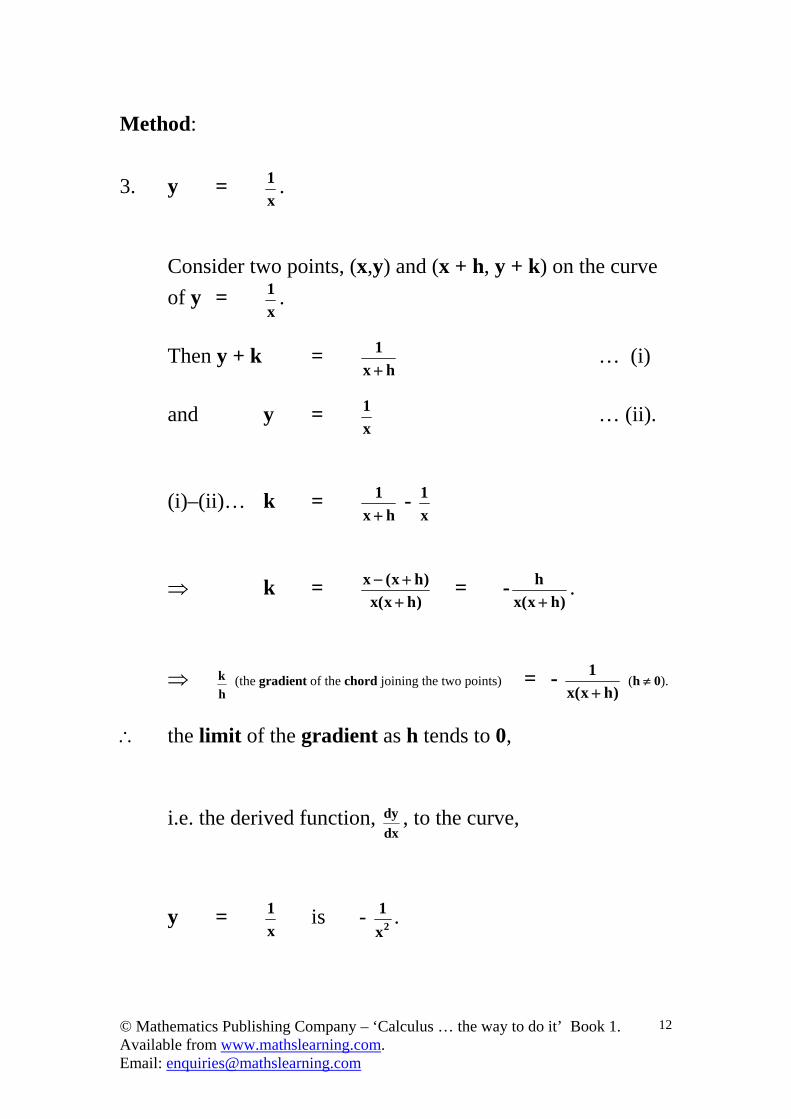
Method:

3. y = x

1 .

Consider two points, (x,y) and (x + h, y + k) on the curve

of y = x

1 .

Then y + k = hx

1

… (i)

and y = x

1 … (ii).

(i)–(ii)… k = hx

1

-

x

1

k = )hx(x

)hx(x

= -

)hx(x

h

.

h

k (the gradient of the chord joining the two points) = - )hx(x

1

(h 0).

the limit of the gradient as h tends to 0,

i.e. the derived function, dx

dy , to the curve,

y = x

1 is - 2x

1 .


13