calendar for the home stretch - mit

Alan Guth, Problems of the Conventional (Non-inflationary) Hot Big Bang Model 8.286 Class 21, November 18, 2020, p. 1.

8.286 Class 21

November 18, 2020

PROBLEMS OF THE

CONVENTIONAL

(NON-INFLATIONARY)

HOT BIG BANG MODEL

(Modified 12/27/20 to fix two typos on p. 10, two typos on p. 16, and oneon p. 19. There are also small clarifications on pp. 21 and 30, and the endof the slides reached in class is marked.)

Calendar for the Home Stretch:

NOVEMBER/DECEMBER

MON TUES WED THURS FRI

16Class 20

17 18Class 21

19 20PS 8 due

23ThanksgivingWeek

24—

25—

26—

27—

30Class 22

December 1 2Class 23Quiz 3

3 4

7Class 24

8 9Class 25PS 9 dueLast Class

10 11

Alan Guth

Massachusetts Institute of Technology

8.286 Class 21, November 18, 2020 –1–

Announcements

For today only, due to an MIT faculty meeting, I am postponing my officehour by one hour, so it will be 5:05-6:00 pm.Problem Set 8 is due this Friday, November 20.Quiz 3 will be on Wednesday, December 2, the Wednesday after theThanksgiving break.It will follow the pattern of the two previous quizzes: Review Problems, a

Review Session, and modified office hours the week of the quiz. Detailsto be announced.

Lecture Notes 8, on the subject of today’s class, will soon be posted.I have posted Notes on Thermal Equilibrium on the Lecture Notes webpage. These are intended as background and clarification for Ryden’ssections on hydrogen recombination and deuterium synthesis. It will notbe covered by Quiz 3, but there will be one or two problems about it onthe last problem set.There will be one last problem set, Problem Set 9, due the last day ofclasses, Wednesday December 9. No final exam!

Alan Guth


8.286 Class 21, November 18, 2020 –2–

Exit Poll, Last Class

Alan Guth


8.286 Class 21, November 18, 2020 –3–


Summary of Last Lecture

Age of the universe with matter, radiation, vacuum energy, and curvature:

t0 =1H0

∫ 1

0

xdx√Ωm,0x+Ωrad,0 +Ωvac,0x4 +Ωk,0x2

.

Look-Back time:

Change variable of integration from x to z, with 1 + z = a(t0)/a(t) = 1/x.Then integrate over z from 0 to zS, the redshift of the source:

tlook-back(zS) =

1H0

∫ zS

0

dz′

(1 + z′)√Ωm,0(1 + z′)3 +Ωrad,0(1 + z′)4 + Ωvac,0 +Ωk,0(1 + z′)2

.

Alan Guth


8.286 Class 21, November 18, 2020 –4–

Review from last class:

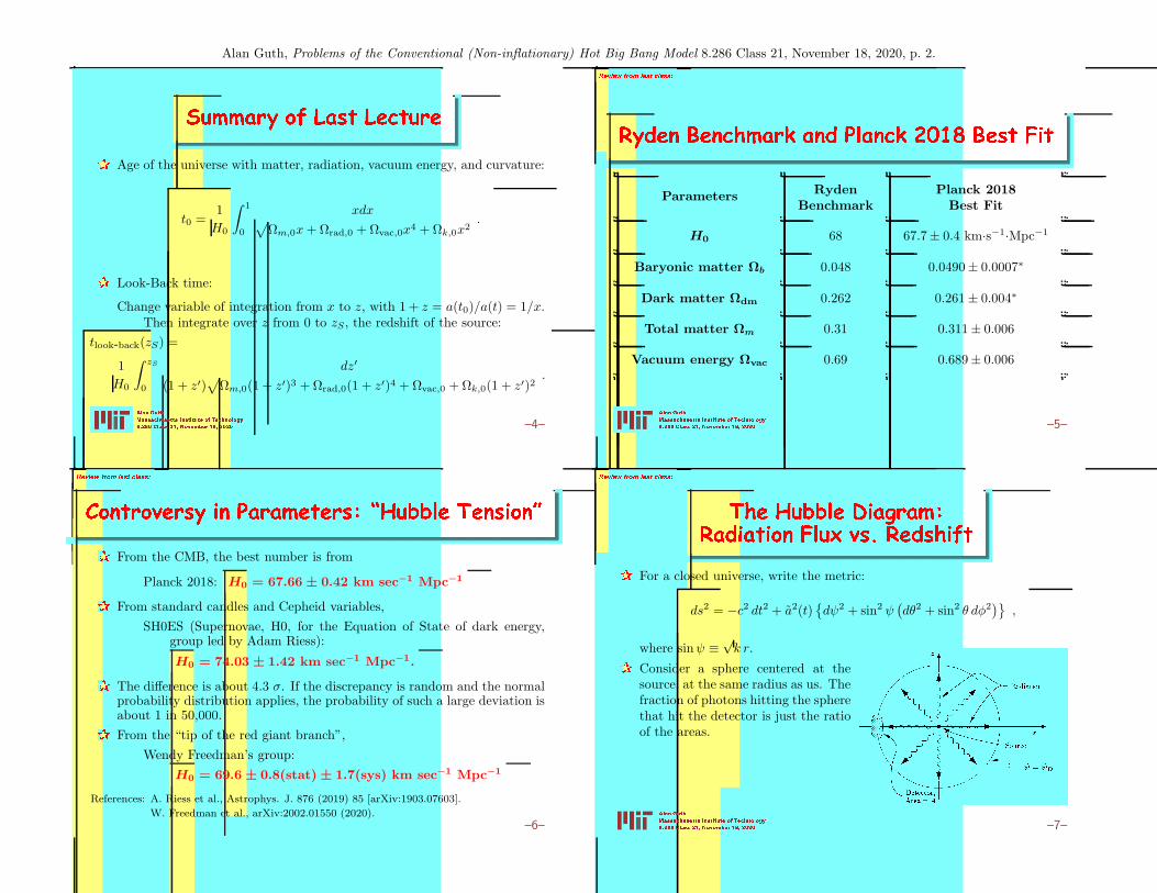
Ryden Benchmark and Planck 2018 Best Fit

Parameters RydenBenchmark

Planck 2018Best Fit

H0 68 67.7± 0.4 km·s−1·Mpc−1

Baryonic matter Ωb 0.048 0.0490± 0.0007∗

Dark matter Ωdm 0.262 0.261± 0.004∗

Total matter Ωm 0.31 0.311± 0.006

Vacuum energy Ωvac 0.69 0.689± 0.006

Alan Guth


8.286 Class 21, November 18, 2020 –5–


Controversy in Parameters: \Hubble Tension"

From the CMB, the best number is from

Planck 2018: H0 = 67.66 ± 0.42 km sec−1 Mpc−1

From standard candles and Cepheid variables,SH0ES (Supernovae, H0, for the Equation of State of dark energy,

group led by Adam Riess):

H0 = 74.03 ± 1.42 km sec−1 Mpc−1.

The difference is about 4.3 σ. If the discrepancy is random and the normalprobability distribution applies, the probability of such a large deviation isabout 1 in 50,000.From the “tip of the red giant branch”,

Wendy Freedman’s group:H0 = 69.6 ± 0.8(stat) ± 1.7(sys) km sec−1 Mpc−1

References: A. Riess et al., Astrophys. J. 876 (2019) 85 [arXiv:1903.07603].

W. Freedman et al., arXiv:2002.01550 (2020).–6–


The Hubble Diagram:

Radiation Flux vs. Redshift

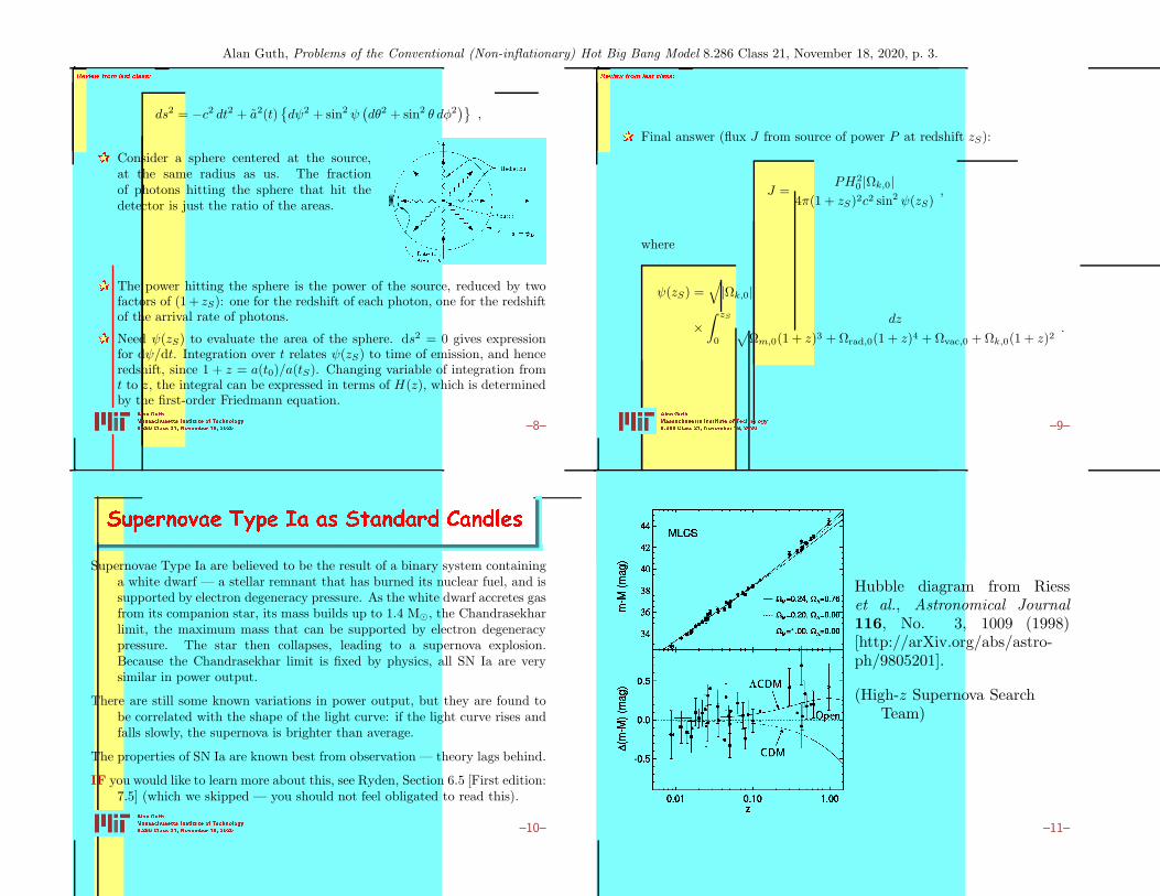
For a closed universe, write the metric:

ds2 = −c2 dt2 + a2(t)dψ2 + sin2 ψ

(dθ2 + sin2 θ dφ2

),

where sinψ ≡ √k r.

Consider a sphere centered at thesource, at the same radius as us. Thefraction of photons hitting the spherethat hit the detector is just the ratioof the areas.

Alan Guth


8.286 Class 21, November 18, 2020 –7–

Alan Guth, Problems of the Conventional (Non-inflationary) Hot Big Bang Model 8.286 Class 21, November 18, 2020, p. 3.Review from last class:

ds2 = −c2 dt2 + a2(t)dψ2 + sin2 ψ

(dθ2 + sin2 θ dφ2

),

Consider a sphere centered at the source,at the same radius as us. The fractionof photons hitting the sphere that hit thedetector is just the ratio of the areas.

The power hitting the sphere is the power of the source, reduced by twofactors of (1+ zS): one for the redshift of each photon, one for the redshiftof the arrival rate of photons.

Need ψ(zS) to evaluate the area of the sphere. ds2 = 0 gives expressionfor dψ/dt. Integration over t relates ψ(zS) to time of emission, and henceredshift, since 1 + z = a(t0)/a(tS). Changing variable of integration fromt to z, the integral can be expressed in terms of H(z), which is determinedby the first-order Friedmann equation.

Alan Guth


8.286 Class 21, November 18, 2020 –8–


Final answer (flux J from source of power P at redshift zS):

J =PH2

0 |Ωk,0|4π(1 + zS)2c2 sin2 ψ(zS)

,

where

ψ(zS) =√|Ωk,0|

×∫ zS

0

dz√Ωm,0(1 + z)3 +Ωrad,0(1 + z)4 +Ωvac,0 +Ωk,0(1 + z)2

.

Alan Guth


8.286 Class 21, November 18, 2020 –9–

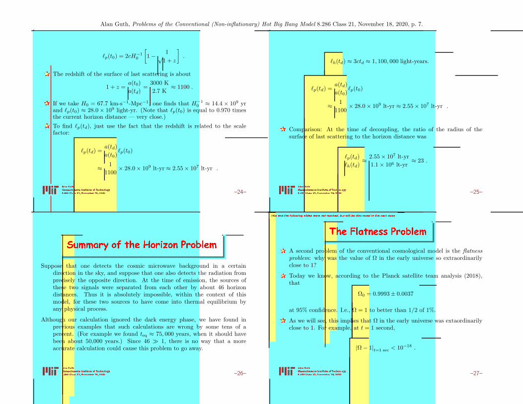
Supernovae Type Ia as Standard Candles

Supernovae Type Ia are believed to be the result of a binary system containinga white dwarf — a stellar remnant that has burned its nuclear fuel, and issupported by electron degeneracy pressure. As the white dwarf accretes gasfrom its companion star, its mass builds up to 1.4 M, the Chandrasekharlimit, the maximum mass that can be supported by electron degeneracypressure. The star then collapses, leading to a supernova explosion.Because the Chandrasekhar limit is fixed by physics, all SN Ia are verysimilar in power output.

There are still some known variations in power output, but they are found tobe correlated with the shape of the light curve: if the light curve rises andfalls slowly, the supernova is brighter than average.

The properties of SN Ia are known best from observation — theory lags behind.

IF you would like to learn more about this, see Ryden, Section 6.5 [First edition:7.5] (which we skipped — you should not feel obligated to read this).

Alan Guth


8.286 Class 21, November 18, 2020 –10–

Hubble diagram from Riesset al., Astronomical Journal116, No. 3, 1009 (1998)[http://arXiv.org/abs/astro-ph/9805201].

(High-z Supernova SearchTeam)

–11–


Dimmer Supernovae Imply Acceleration

The acceleration of the universe is deduced from the fact that distantsupernovae appear to be 20-30% dimmer than expected.

Why does dimness imply acceleration?

• Consider a supernova of specified apparent brightness.

• “Dimmer” implies data point is to the left of where expected — atlower z.

• Lower z implies slower recession, which implies that the universe wasexpanding slower than expected in the past — hence, acceleration!

Alan Guth


8.286 Class 21, November 18, 2020 –12–

Other Possible Explanations for Dimness

Absorption by dust.

• But absorption usually reddens the spectrum. This would haveto be “gray” dust, absorbing uniformly at all observed wavelengths.Such dust is possible, but not known to exist anywhere.

• Dust would most likely be in the host galaxy, which would causevariable absorption, depending on SN location in galaxy. Suchvariability is not seen.

Chemical evolution of heavy element abundance.• But nearby and distant SN Ia look essentially identical.• For nearby SN Ia, heavy element abundance varies, and does notappear to affect brightness.

Additional evidence against dust or chemical evolution: A SN Ia has beenfound at z = 1.7, which is early enough to be in the decelerating era of thevacuum energy density model. It is consistent with deceleration, but notconsistent with either models of absorption or chemical evolution.

Alan Guth


8.286 Class 21, November 18, 2020

–13–

Evidence for the Accelerating Universe

1) Supernova Data: distant SN Ia are dimmer than expected by about 20–30%.

2) Cosmic Microwave Background (CMB) anisotropies: gives Ωvac close to SNvalue. Also gives Ωtot = 1 to 1/2% accuracy, which cannot be accountedfor without dark energy.

3) Inclusion of Ωvac ≈ 0.70 makes the age of the universe consistent with theage of the oldest stars.

With the 3 arguments together, the case for the accelerating universe andΩdark energy ≈ 0.70 has persuaded almost everyone.

The simplest explanation for dark energy is vacuum energy, but“quintessence” is also possible.

Alan Guth


8.286 Class 21, November 18, 2020 –14–

Particle Physics of a Cosmological Constant

uvac = ρvacc2 =

Λc4

8πG

Contributions to vacuum energy density:

1) Quantum fluctuations of the photon and other bosonic fields: positiveand divergent.

2) Quantum fluctuations of the electron and other fermionic fields:negative and divergent.

3) Fields with nonzero values in the vacuum, like the Higgs field.

Alan Guth


8.286 Class 21, November 18, 2020 –15–


If infinities are cut off at the Planck scale (quantum gravity scale), theninfinities become finite, but

> 120 orders of magnitude too large!

For lack of a better explanation, many cosmologists (including SteveWeinberg and yours truly) seriously discuss the possibility that the vacuumenergy density is determined by “anthropic” selection effects: that is,maybe there are many types of vacuum (as predicted by string theory),with different vacuum energy densities, with most vacuum energy densitiesroughly 120 orders of magnitude larger than ours. Maybe we live in a verylow energy density vacuum because that is where almost all living beingsreside. A large vacuum energy density would cause the universe to rapidlyfly apart (if positive) or implode (if negative), so life could not form.

Alan Guth


8.286 Class 21, November 18, 2020 –16–

8.286 Class 21

November 18, 2020

PROBLEMS OF THE

CONVENTIONAL

(NON-INFLATIONARY)

HOT BIG BANG MODEL

–17–

The Horizon/Homogeneity Problem

General question: how can we explain the large-scale uniformity of theuniverse?

Possible answer: maybe the universe just started out uniform.

• There is no argument that excludes this possibility, since we don’tknow how the universe came into being.

• However, if possible, it seems better to explain the properties of theuniverse in terms of things that we can understand, rather than toattribute them to things that we don’t understand.

Alan Guth


8.286 Class 21, November 18, 2020 –18–

The Horizon in Cosmology

The concept of a horizon was first introduced into cosmology by WolfgangRindler in 1956.

The “horizon problem” was discussed (not by that name) in at leasttwo early textbooks in general relativity and cosmology: Weinberg’sGravitation and Cosmology (1972), and Misner, Thorne, and Wheeler’s(MTW’s) Gravitation (1973).

Alan Guth


8.286 Class 21, November 18, 2020 –19–


The Cosmic Microwave Background

The strongest evidence for the uniformity of the universe comes from theCMB, since it has been measured so precisely.

The radiation appears slightly hotter in one direction than in the oppositedirection, by about one part in a thousand — but this nonuniformity canbe attributed to our motion through the background radiation.

Once this effect is subtracted out, using best-fit parameters for the velocity,it is found that the residual temperature pattern is uniform to a few partsin 105.

Could this be simply the phenomenon of thermal equilibrium? If you putan ice cube on the sidewalk on a hot summer day, it melts and come stothe same temperature as the sidewalk.

BUT: in the conventional model of the universe, it did not haveenough time for thermal equilibrium to explain the uniformity, ifwe assume that it did not start out uniform. If no matter, energy,or information can travel faster than light, then it is simply notpossible.

Alan Guth


8.286 Class 21, November 18, 2020 –20–

Basic History of the CMB

In conventional cosmological model, the universe at the earliest times wasradiation-dominated. It started to be matter-dominated at teq ≈ 50, 000years, the time of matter-radiation equality.

At the time of decoupling td ≈ 380, 000 years, the universe cooled toabout 3000 K, by which time the hydrogen (and some helium) combined sothoroughly that free electrons were very rare. At earlier times, the universewas in a mainly plasma phase, with many free electrons, and photonswere essentially frozen with the matter. At later times, the universe wastransparent, so photons have traveled on straight lines. We can say thatthe CMB was released at about 380,000 years.

Since the photons have been mainly traveling on straight lines since t = td,they have all traveled the same distance. Therefore the locations fromwhich they were released form a sphere centered on us. This sphere iscalled the surface of last scattering, since the photons that we receive nowin the CMB was mostly scattered for the last time on or very near thissurface.

Alan Guth


8.286 Class 21, November 18, 2020 –21–

As we learned in Lecture Notes 4, the horizon distance is defined as thepresent distance of the furthest particles from which light has had time toreach us, since the beginning of the universe.

For a matter-dominated flat universe, the horizon distance at time t is 3ct,while for a radiation-dominated universe, it is 2ct.

At t = td the universe was well into the matter-dominated phase, so wecan approximate the horizon distance as

h(td) ≈ 3ctd ≈ 1, 100, 000 light-years.

For comparison, we would like to calculate the radius of the surface of lastscattering at time td, since this region is the origin of the photons thatwe are now receiving in the CMB. I will denote the physical radius of thesurface of last scattering, at time t, as p(t).

Alan Guth


8.286 Class 21, November 18, 2020 –22–


For comparison, we would like to calculate the radius of the surface of lastscattering at time td, since this region is the origin of the photons that we arenow receiving in the CMB. I will denote the physical radius of the surface oflast scattering, at time t, as p(t).

To calculate p(td), I will make the crude approximation that the universehas been matter-dominated at all times. (We will find that this horizonproblem is very severe, so even if our calculation is wrong by a factor of 2,it won’t matter.)

Strategy: find p(t0), and scale to find p(td). Under the assumption ofa flat matter-dominated universe, we learned that the physical distancetoday to an object at redshift z is

p(t0) = 2cH−10

[1− 1√

1 + z

].

Alan Guth


8.286 Class 21, November 18, 2020 –23–


p(t0) = 2cH−10

[1− 1√

1 + z

].

The redshift of the surface of last scattering is about

1 + z =a(t0)a(td)

=3000 K2.7 K

≈ 1100 .

If we take H0 = 67.7 km-s−1-Mpc−1, one finds that H−10 ≈ 14.4× 109 yr

and p(t0) ≈ 28.0× 109 light-yr. (Note that p(t0) is equal to 0.970 timesthe current horizon distance — very close.)

To find p(td), just use the fact that the redshift is related to the scalefactor:

p(td) =a(td)a(t0)

p(t0)

≈ 11100

× 28.0× 109 lt-yr ≈ 2.55× 107 lt-yr .

Alan Guth


8.286 Class 21, November 18, 2020 –24–


p(td) =a(td)a(t0)

p(t0)

≈ 11100

× 28.0× 109 lt-yr ≈ 2.55× 107 lt-yr .

Comparison: At the time of decoupling, the ratio of the radius of thesurface of last scattering to the horizon distance was

p(td)h(td)

≈ 2.55× 107 lt-yr1.1× 106 lt-yr

≈ 23 .

Alan Guth


8.286 Class 21, November 18, 2020 –25–

Summary of the Horizon Problem

Suppose that one detects the cosmic microwave background in a certaindirection in the sky, and suppose that one also detects the radiation fromprecisely the opposite direction. At the time of emission, the sources ofthese two signals were separated from each other by about 46 horizondistances. Thus it is absolutely impossible, within the context of thismodel, for these two sources to have come into thermal equilibrium byany physical process.

Although our calculation ignored the dark energy phase, we have found inprevious examples that such calculations are wrong by some tens of apercent. (For example we found teq ≈ 75, 000 years, when it should havebeen about 50,000 years.) Since 46 1, there is no way that a moreaccurate calculation could cause this problem to go away.

Alan Guth


8.286 Class 21, November 18, 2020 –26–

This and the following slides were not reached, but will be discussed in the next class.

The Flatness Problem

A second problem of the conventional cosmological model is the flatnessproblem: why was the value of Ω in the early universe so extraordinarilyclose to 1?

Today we know, according to the Planck satellite team analysis (2018),that

Ω0 = 0.9993± 0.0037

at 95% confidence. I.e., Ω = 1 to better than 1/2 of 1%.

As we will see, this implies that Ω in the early universe was extaordinarilyclose to 1. For example, at t = 1 second,

|Ω− 1|t=1 sec < 10−18 .

Alan Guth


8.286 Class 21, November 18, 2020 –27–


The underlying fact is that the value Ω = 1 is a point of unstableequilibrium, something like a pencil balancing on its point. If Ω is everexactly equal to one, it will remain equal to one forever — that is, a flat(k = 0) universe remains flat. However, if Ω is ever slightly larger thanone, it will rapidly grow toward infinity; if Ω is ever slightly smaller thanone, it will rapidly fall toward zero. For Ω to be anywhere near 1 today, Ωin the early universe must have been extraordinarily close to one.

Like the horizon problem, the flatness problem could in principle be solvedby the initial conditions of the universe: maybe the universe began withΩ ≡ 1.

• But, like the horizon problem, it seems better to explain the propertiesof the universe, if we can, in terms of things that we can understand,rather than to attribute them to things that we don’t understand.

Alan Guth


8.286 Class 21, November 18, 2020 –28–

History of the Flatness Problem

The mathematics behind the flatness problem was undoubtedly known to almostanyone who has worked on the big bang theory from the 1920’s onward, butapparently the first people to consider it a problem in the sense describedhere were Robert Dicke and P.J.E. Peebles, who published a discussion in1979.∗

∗R.H. Dicke and P.J.E. Peebles, “The big bang cosmology — enigmas and nostrums,” inGeneral Relativity: An Einstein Centenary Survey, eds: S.W. Hawking and W.Israel, Cambridge University Press (1979).

Alan Guth


8.286 Class 21, November 18, 2020 –29–

The Mathematics of the Flatness Problem

Start with the first-order Friedmann equation:

H2 ≡(a

a

)2

=8π3Gρ− kc2

a2.

Remembering that Ω = ρ/ρc and that ρc = 3H2/(8πG), one can divideboth sides of the equation by H2 to find

1 =ρ

ρc− kc2

a2H2=⇒ Ω − 1 =

kc2

a2H2.

Alan Guth


8.286 Class 21, November 18, 2020 –30–

Evolution of Ω − 1 During

the Radiation-Dominated Phase

Ω− 1 =kc2

a2H2.

For a (nearly) flat radiation-dominated universe, a(t) ∝ t1/2, so H = a/a =1/(2t). So

Ω− 1 ∝(

1t1/2

)2 (1t−1

)2

∝ t (radiation dominated).

Alan Guth


8.286 Class 21, November 18, 2020 –31–


Evolution of Ω − 1 During

the Matter-Dominated Phase

Ω− 1 =kc2

a2H2.

For a (nearly) flat matter-dominated universe, a(t) ∝ t2/3, soH = a/a = 2/(3t).So

Ω− 1 ∝(

1t2/3

)2 (1t−1

)2

∝ t2/3 (matter-dominated).

Alan Guth


8.286 Class 21, November 18, 2020 –32–

Tracing Ω − 1 from

Now to 1 Second

Today,

|Ω0 − 1| < .01 .

I will do a crude calculation, treating the universe as matter dominated from50,000 years to the present, and as radiation-dominated from 1 second to50,000 years.

During the matter-dominated phase,

(Ω− 1)t=50,000 yr ≈(

50,00013.8× 109

)2/3

(Ω0 − 1) ≈ 2.36× 10−4 (Ω0 − 1) .

Alan Guth


8.286 Class 21, November 18, 2020 –33–

|Ω0 − 1| < .01 .

(Ω − 1)t=50,000 yr ≈(

50,00013.8× 109

)2/3

(Ω0 − 1) ≈ 2.36× 10−4 (Ω0 − 1) .

During the radiation-dominated phase,

(Ω− 1)t=1 sec ≈(

1 sec50,000 yr

)(Ω− 1)t=50,000 yr

≈ 1.49× 10−16 (Ω0 − 1) .

The conclusion is therefore

|Ω− 1|t=1 sec < 10−18 .

Alan Guth


8.286 Class 21, November 18, 2020

–34–

The conclusion is therefore

|Ω− 1|t=1 sec < 10−18 .

Even if we put ourselves mentally back into 1979, we would have said that0.1 < Ω0 < 2, so |Ω0 − 1| < 1, and would have concluded that

|Ω− 1|t=1 sec < 10−16 .

The Dicke & Peebles paper, that first pointed out this problem, also consideredt = 1 second, but concluded (without showing the details) that

|Ω− 1|t=1 sec < 10−14 .

They were perhaps more conservative, but concluded nonetheless that thisextreme fine-tuning cried out for an explanation.

Alan Guth


8.286 Class 21, November 18, 2020 –35–

calendar for the home stretch - mit

Documents