calibration inspired by semiparametric regression as a ... · calibration inspired by...

Calibration Inspired by Semiparametric Regressionas a Treatment for Nonresponse

Giorgio E. Montanari1 and M. Giovanna Ranalli2

In the last decade, calibration has been used to reduce both sampling error and nonresponsebias in surveys. In the presence of auxiliary variables with known population totals or withknown values on the originally sampled units, the calibration procedure generates finalweights for observations that, when applied to those auxiliary variables, yield their populationtotals or unbiased estimates of these totals, respectively. A single set of variables and a singlecalibration step is employed to this end. In this article, we extend this approach to allow formore flexible implicit description of the relationship of the auxiliary variables with either theresponse probabilities or the survey variable(s). By using penalized splines the simplicity ofthe original proposal and the linearity of the estimator are preserved. The conditions underwhich the proposed estimator of the total is design consistent and its asymptotic properties areexplored, and its finite sample behavior is investigated via simulations.

Key words: Auxiliary information; nonparametric regression; penalized splines; nonresponsebias; shrinkage; unit nonresponse.

1. Introduction

Nonresponse can harm the quality of the estimates of a survey. In particular, since we have

to accept that those who respond are in general different from those who do not respond,

bias is introduced. In this article we will not deal with imputation, but only with design

weights modification to adjust for unit nonresponse bias. Note that techniques for handling

nonresponse can be employed also for nonresponse adjustments in censuses. Commonly, a

two-phase approach is used, with the response mechanism as the second phase; this is

based on quasi-randomization theory, where the response distribution has corresponding

response probabilities assumed to be independent of the realized sample (e.g., Sarndal et al.

1992, Ch. 9). In practice, such response probabilities have to be estimated assuming a

response model. The prefix “quasi” is added to emphasize that inference depends not only

on the design, but also on the assumed response model.

q Statistics Sweden

1 Dipartimento di Economia, Finanza e Statistica, Universita degli Studi di Perugia. Email: [email protected] Dipartimento di Economia, Finanza e Statistica, Universita degli Studi di Perugia. Email: [email protected]: This study was first presented as an invited paper at the First Italian Conference on SurveyMethodology, Siena, Italy, June 10-12, 2009. The work reported here has been developed under the support of theproject PRIN 2007 “Efficient use of auxiliary information at the design and at the estimation stage of complexsurveys: methodological aspects and applications for producing official statistics” awarded by the ItalianGovernment. The authors wish to thank the associate editor and three referees for their close reading of themanuscript and for many thoughtful comments, Wayne Fuller and Mingue Park for very useful suggestions onsome theoretical issues.

Journal of Official Statistics, Vol. 28, No. 2, 2012, pp. 239–277

One of the most common and simple techniques for handling nonresponse is given by

constructing response homogeneity groups: the population (or the sample) can be

partitioned into groups in such way that units belonging to the same group are assumed to

have the same response probability. Sometimes, a more complex direct modeling of the

response probabilities is conducted, for example through logistic regression models (Little

1986; Ekholm and Laaksonen 1991). Asymptotic properties in this situation are explored

in Kim and Kim (2007). More generally, the probability of response can be assumed to be

the inverse of a known link function of an unknown (but estimable) linear combination of

model variables (Folsom 1991; Fuller et al. 1994; Kott 2006). Nonparametric regression

that allows relaxing the assumption of a known functional relationship between response

probabilities and model variables has been explored through kernel smoothing (Giommi

1987; Silva and Opsomer 2006).

Lundstrom and Sarndal (1999) propose a simple approach for the treatment of

nonresponse based on calibration (Deville and Sarndal 1992). This is pursued by the

construction of a single set of weights for all variables of interest that are as close as

possible to specified initial weights (usually the design weights), while satisfying

benchmark constraints on known auxiliary information. No discrimination is made within

the set of auxiliary variables available to the researcher: a single set of variables is

employed at the same time for nonresponse treatment, sampling error reduction and

coherence among estimates. No explicit model is specified for the treatment of the

nonresponse mechanism; it is implicitly given by the calibration procedure.

The relationship between regression estimation and calibration is well known (Deville

and Sarndal 1992; Sarndal 2007): the efficiency of the calibration procedures relies on how

well a linear model describes the relationship between the variable(s) of interest and the

auxiliary ones. It therefore may be inefficient when the underlying relationship is indeed

nonlinear (Wu and Sitter 2001; Montanari and Ranalli 2005). We argue that the approach in

Lundstrom and Sarndal (1999) can be usefully generalized to include more complex

relationships through semiparametric regression (Rupper et al. 2003) without losing in

simplicity. Semiparametric regression based on penalized splines (Eilers and Marx 1996)

has been usefully employed for model-assisted inference in the case of complete response

(Breidt et al. 2005). More easily than with kernel smoothing, it allows for the treatment, at

the same time, of categorical and continuous auxiliary variables. Categorical variables can

be inserted parametrically, while continuous variables can be accounted for nonparame-

trically. Recently, a kernel-based model-assisted estimator that can handle both continuous

and categorical covariates has been proposed in Sanchez-Borrego et al. (2011).

The article proceeds as follows: in Section 2, calibration with particular regards to

treatment of nonresponse is reviewed. In Section 3, semiparametric regression is employed

to extend nonparametrically calibration to the treatment of nonresponse. Simulation studies

that explore the finite sample behavior of the proposed estimator are reported in Section 4.

Some concluding remarks and directions for future research are provided in Section 5.

2. Calibration as a Treatment for Nonresponse

Consider a finite population of N elements U ¼ {1; : : : ; k; : : : ;N}; the aim is to estimate

the total Y ¼P

U yk, where yk is the value of the variable of interest y for the kth unit.

Journal of Official Statistics240

We will use the shorthandP

A forP

k[A, with A # U an arbitrary set. A sample s of size n

is drawn from U through the sampling design p(s) that induces positive first and second

order inclusion probabilities pk ¼ Pðk [ sÞ and pkj ¼ Pðk; j [ sÞ, respectively, with

pkk ¼ pk. Let Ik be the indicator variable for unit k selected in the sample, so that

EðIkjF Þ ¼ pk, where F ¼ {u1; : : : ; uN}; uk ¼ yk; xTk

� �, and xk is the value of the

p-vector of auxiliary variables x on unit k. Therefore, expectation is taken with respect to

the sampling design and conditional of the realized finite population F . We will denote

with dk ¼ 1=pk the design weight of unit k. Since nonresponse occurs, the response set r of

size m is obtained, with r # s and m # n. Let dk ¼ 1 if unit k responds and 0 otherwise.

Lundstrom and Sarndal (1999) consider auxiliary information on two separate levels. In

particular, x is considered a vector of auxiliary variables assumed to contain information

for reducing both the sampling error and the nonresponse bias, and the two following

“information levels” are considered:

info-s: xk is known for all k [ s;

info-U: xk is observed for all k [ r andP

U xk is known.

In the first case, information goes up to the sample level, while in the second case, it refers

to the population. A combination of the two can of course be considered (Sarndal and

Lundstrom 2005), but we will consider them separately in order to keep this discussion

simple.

Design weights dk for responding units are on average too small to produce reasonable

Horvitz-Thompson estimates of totals when there is nonresponse. They need to be

adjusted by a factor vk. Calibrated weights wk ¼ dkvk used to compute the estimator

Yc;r ¼P

r wkyk of Y are obtained so that they satisfy calibration equations given by either

info-s:P

r wkxk ¼P

s dkxk, or

info-U:P

r wkxk ¼P

U xk.

A simple choice for the factors vk may be vk ¼ 1 þ jTxk, which is linear and has

considerable computational advantages. Note that this choice is equivalent to finding

calibrated weights by minimizing a chi-squared distance measure from basic design

weights (see e.g. Deville and Sarndal 1992; Sarndal and Lundstrom 2005, p. 58). Other

forms for vk are considered in Deville (2000) and Kott (2006). The vector j is determined

after substitution in the calibration equations. The calibration estimator in these cases

takes the following forms:

info-s: Yc;r ¼P

r dkvskyk, with

vsk ¼ 1 þs

Xdkxk 2

r

Xdkxk

!T

r

Xdkxkx

Tk

!21

xk; for k [ r;

info-U: Yc;r ¼P

r dkvUkyk, with

vUk ¼ 1 þU

Xxk 2

r

Xdkxk

0@

1A

T

r

Xdkxkx

Tk

!21

xk; for k [ r: ð1Þ

Montanari and Ranalli: Semiparametric Regression for Nonresponse Treatment 241

Note that the estimator is constructed using calibration in a single phase and without

explicit introduction of a model for the response mechanism. In addition, the weights do

not depend on the study variable y, and therefore the estimator is said to be linear. Such a

property is very valuable in a survey setting, because the calibrated weights can then be

applied to all variables of interest. Poststratification is included as a special case of Yc;r if

the auxiliary vector xk denotes membership to poststrata. In case of full response, when

r ¼ s, Yc;s ¼P

s dkyk, that is, the Horvitz-Thompson estimator for info-s, and

Yc;s ¼P

s dkgc;kyk, with gc;k ¼ 1 þP

U xk 2P

s dkxk� �T P

s dkxkxTk

� �21xk, that is, the

generalized regression estimator for info-U.

In the two-phase approach to handling nonresponse, an unbiased estimator is given by

Y2p ¼r

X dk

ukyk ð2Þ

where uk ¼ Pðdk ¼ 1jIk ¼ 1Þ is the conditional probability that unit k responds, given that

the unit is selected in the sample (Sarndal et al. 1992, Ch. 9). Of course such estimator

cannot be computed, since nonresponse probabilities are not known. However, we can

note that Yc;r uses proxy values given by vsk and vUk to approximate u21k , that is, the inverse

of the response probability for unit k is implicitly approximated by a linear combination of

the vector of auxiliary variables xk.

Weights in (1) provide a calibration estimator that is equivalent to the regression

estimator in the presence of nonresponse. In fact, it can be written in the form

Yc;r ¼r

Xdkyk þ

�U

Xxk 2

r

Xdkxk

�Tbr; ð3Þ

where br ¼P

r dkxkxTk

� �21Pr dkxkyk, that is, the regression estimator when the regres-

sion coefficient is computed only on respondents. This estimator has been considered and

studied in Fuller et al. (1994) and Fuller and An (1998).

To review the large sample properties of Yc;r, we will consider the traditional finite

population asymptotic framework considered in Isaki and Fuller (1982), where

the population U and the sampling design p(·) are embedded into a sequence of finite

populations and associated probability samples. The set of indices of the elements in the

Nth finite population is UN ¼ {1; 2; : : : ;N} with N ¼ pþ 1; pþ 2; : : :, while the design

is pN(·) and the sample size nN is assumed to grow with N. Let FN ¼

y1N ; xT1N

� �; y2N ; x

T2N

� �; : : : ; yNN ; x

TNN

� �� be the set of vectors of both survey and

auxiliary variables for the Nth finite population. In the following, the subscript N on the

vectors will often be dropped for ease of notation.

Now, under regularity conditions such as those reported in Fuller (2002), br is a design-

consistent estimator of

cU ¼U

Xukxkx

Tk

0@

1A21

U

Xukxkyk; ð4Þ


in the sense that, given FN for all N . p þ 2, lim N!1P{jbr 2 cU j . ejFN} ¼ 0

for all e . 0. The population total of y can be written as

Y ¼U

Xak þ

U

XxTk cU

with ak ¼ yk 2 xTk cU . Therefore, the regression estimator in (3) – and consequently Yc;rfor info-U – will be a design-consistent estimator for Y, in the sense that

lim N!1P{jYc;r 2 Yj . Ne jFN} ¼ 0, if the probability limit ofP

U ak is zero. There

are several ways in which this occurs. Fuller et al. (1994) give the three following

situations.

(i) The probability limit ofP

U ak is zero when the sequence of finite populations is a

sequence of random samples from an infinite population in which the linear model

yk ¼ xTk bþ ek, with the ek independent of the xk and with zero expectation, holds for

all k.

(ii) The totalP

U ak is zero when uk is constant for all k, because in this case

cU ¼ bU ¼P

U xkxTk

� �21PU xkyk, and

PU yk 2 xTk bU ¼ 0.

(iii) A sufficient condition forP

U ak to be zero is the existence of a vector d such that

xTk d ¼ u21k ð5Þ

for all k [ U. Therefore, if the inverse of the response probability is a linear function

of the auxiliary variables, the regression estimator is consistent for Y.

Note that to have design consistency, it is sufficient that any one of these conditions holds.

Apart from condition (ii ), which is unlikely to hold in practice, it is enough that the

auxiliary variables fulfill either the prediction model in (i ) or the response model in (iii ) to

achieve a vanishing bias. This property has been called “double protection” against

nonresponse bias.

The third condition sheds some light on the implicit modeling of the response

mechanism done with the one-step calibration technique. A sufficient condition for

consistency is that the inverse of the response probabilities belongs to the space spanned by

the columns of the N £ p matrix of population values of x. In the following section, the

approach in Lundstrom and Sarndal (1999) is generalized to make condition (i ) above valid

for a wider range of models through semiparametric regression without loss of simplicity.

3. Calibration Inspired by Semiparametric Regression for the Treatment of

Nonresponse

Semiparametric regression that relies on penalized splines has been usefully employed for

model-assisted inference in the case of complete response (Breidt et al. 2005). Penalized

splines are now often referred to as p-splines and have been brought to attention by Eilers

and Marx (1996). P-splines provide an attractive smoothing method due to their simplicity

of implementation, being a relatively straightforward extension of linear regression, and to

their flexibility, as they are applicable in a wide range of modeling contexts. Ruppert et al.

(2003) provide a thorough treatment of p-splines and their applications. In this section,


we first describe p-splines in the general context of model-assisted estimation regardless of

nonresponse, and then move to semiparametric regression-based calibration for treatment

of nonresponse.

3.1. Review of p-splines for Model-Assisted Regression Estimation

Let us first consider only smoothing with one covariate z. In Breidt et al. (2005), a

nonparametric superpopulation regression model is written as

yk ¼ mðzkÞ þ 1k; ð6Þ

where the errors 1k are independent random variables with mean zero and variance v(zk).

The p-spline estimator of the unknown function m(·) may be given by

mðz;bÞ ¼ b0 þ b1zþXLl¼1

b1þlðz2 klÞþ ð7Þ

where the so-called plus functions (t)þ are such that (t)þ ¼ t if t . 0 and 0 otherwise (see

Figure 1), kl for l ¼ 1; : : : ; L is a set of fixed knots, b ¼ ðb0;b1; : : : ;b1þLÞT is the

coefficient vector made of a parametric portion (the first two coefficients) and a spline part

(the last L coefficients). The latter portion of the model allows for handling departures

from a linear fit in the structure of the relationship. If the number of knots L is sufficiently

large, the class of functions in (7) is very large and can approximate most smooth

functions. In the p-splines context, a knot is placed every 4 or 5 observations; however, to

avoid an excessive number of knots (and therefore parameters), a maximum number of

allowable knots, say 35, is recommended. In addition, knots are usually placed at the

quantiles of the distribution of z, making unequally spaced intervals so as to more properly

account for the possible skewness of such a distribution. More details on knots choice can

be found in Ruppert et al. (2003, Ch. 3 and 5). In the survey context, the choice of the

2.0 Plus functionDerivative1.8

1.6

1.4

1.2

1.0

0.8

0.6

0.4

0.2

0

0 0.5 1 1.5 2 2.5 3

Fig. 1. Example of a truncated linear spline basis (x 2 k)þ with k ¼ 1 (solid line) and of its derivative

(dashed line).


location of the knots may be also influenced by the available population level auxiliary

information. More details on this aspect will be given in Section 3.2.

The spline model (7) uses a truncated linear spline basis to approximate the function

m(·). In this case, the slope of the relationship between y and z is allowed to change when it

hits a knot. The amount of the change is given by the coefficient of the corresponding base

function, which represents the change in the first derivative of the approximating function

at the knot (see Figure 1). Truncated polynomials of higher order, say 2 or 3, can be used,

in which, similarly, coefficients for the base functions provide the change in the 2nd and

3rd, respectively, derivative. Different bases can be used, like thin plate splines or

B-splines; more details on choice of base can be found in Ruppert et al. (2003, Ch. 3 and

5). In this article we will use p-splines with a truncated linear basis, not only for their

simplicity of interpretation, but also because of their implication on the auxiliary

information required. We will see this in more detail in the next section.

Given the large number of knots, model (7) can be too complex; the influence of the

knots can be limited by putting a constraint on the size of the spline coefficients.

Estimation can be accommodated by including this constraint in the least squares criterion,

so that the census level estimator of the parameter vector is given by the minimizer of

U

X{yk 2 mðzk;bÞ}

2 þ lXLl¼1

b21þl

for some fixed positive constant l. The smoothness of the resulting fit depends on the value

of l, with larger values corresponding to smoother fits. Choice of l will be discussed later.

Let zk ¼ ð1; zk; ðzk 2 k1Þþ; : : : ; ðzk 2 kLÞþÞT and L ¼ diag{0; 0; l; : : : ; l} be an L þ 2

diagonal matrix. Then, the census level penalized least squares estimator of the coefficient

vector has the following ridge regression representation

bU ¼U

Xzkz

Tk þL

0@

1A

21

U

Xzkyk:

The role of the matrix L is to shrink the magnitude of the value of the coefficient bU for

the spline part of the function in (7). Under the conditions in Breidt et al. (2005), consistent

design-based estimates of bU can be obtained as bs ¼P

s dkzkzTk þL

� �21Ps dkzkyk.

Finally, sample-based fits mk ¼ mðzk; bsÞ are used to define the model-assisted p-spline

estimator

Yp;s ¼U

Xmk þ

s

Xdkð yk 2 mkÞ ¼

s

Xdkgp;kyk ð8Þ

with gp;k ¼ 1 þP

U zk 2P

s dkzk� �T P

s dkzkzTk þL

� �21zk. Breidt et al. (2005, Sec. 2.2)

discuss in detail the properties of this estimator. Here note that it can be seen as a

calibration estimator in which calibration constraints are met for the first two variables

{1, z} and are relaxed for the other L. The amount of relaxation depends on the smoothing

parameter l. Relaxing the constraints on the L variables related to the knots has a

shrinkage effect on the range of the final set of weights.


3.2. P-splines and Calibration for the Treatment of Nonresponse

Now, we want to exploit the enhanced flexibility provided by using p-splines in a model-

assisted framework while retaining the simplicity of the proposal of Lundstrom and

Sarndal (1999) for handling nonresponse. To achieve this, we introduce the following

calibration estimator based on p-splines:

info-s: Yp;r ¼P

r dkvskyk, with

vsk ¼ 1 þs

Xdkzk 2

r

Xdkzk

!T

r

Xdkzkz

Tk þL

!21

zk; ð9Þ

info-U: Yp;r ¼P

r dkvUkyk, with

vUk ¼ 1 þU

Xzk 2

r

Xdkzk

0@

1A

T

r

Xdkzkz

Tk þL

!21

zk: ð10Þ

It is easy to see that in the case of full response, that is, when r ¼ s, Yp;r reduces to the

Horvitz-Thompson estimator for info-s and to Yp;s in (8) for info-U. Recall that the

auxiliary information for unit k used to compute these estimators is given by

zk ¼ 1; zk; z*Tk

� �T, with z*

k ¼ ððzk 2 k1Þþ; : : : ; ðzk 2 kLÞþÞT . The first two entries of the

vector are those usually employed for calibration, while z*k allows for handling departures

from a linear fit in the structure of the relationship between y and z as illustrated in the

previous section. Calibrating on the whole vector zk, however, may lead to a very erratic

final set of weights. Therefore, the influence of the knots is limited by relaxing the binding

constraint for that part of the auxiliary information. This is accomplished by minimizing a

penalized version of the chi-square distance measure between final and initial weights. In

particular, weights satisfy either of the two following conditions:

info–s : min wkr

X ðwk 2 dkÞ2

dkþ

r

Xwkz

*k 2

s

Xdkz

*k

!T

L21*

r

Xwkz

*k 2

s

Xdkz

*k

!

under the constraintXr

wkð1; zkÞ ¼Xs

dkð1; zkÞ;

info–U : min wkr

X ðwk 2 dkÞ2

dkþ

r

Xwkz

*k 2

U

Xz*k

0@

1A

T

L21*

r

Xwkz

*k 2

U

Xz*k

0@

1A

under the constraintXr

wkð1; zkÞ ¼XU

ð1; zkÞ;

where L* ¼ diag{l; : : : ; l} and l here represents the inverse cost of relaxing those

constraints. In general, smaller values of l mean a large penalization and therefore that the

calibration constraints are more stringent. Larger values imply increasingly relaxing the

constraint for those variables and, therefore, a shrinkage effect on the range of the final set

of weights. The results of those constrained minimization problems provide the estimators


considered above. See also Rao and Singh (1997) on relaxing the calibration constraints,

and Fuller (2002, Sec. 9), Park and Fuller (2009) and Guggemos and Tille (2010) on the

link between the penalized minimum distance criterion and mixed effects models, and

Beaumont and Bocci (2008) for a review on ridge calibration.

Let us consider again the estimator under the two-phase approach to handling

nonresponse in (2). Here, for Yp;r we can see that the inverse of the response probability is

approximated by proxy values given by vUk and vsk for info-U and info-s respectively,

which depend on the whole vector of auxiliary variables zk and not only on its linear part

(1, zk) as it would be the case under classical calibration estimation. This allows for a more

flexible implicit description of the nonresponse mechanism.

Let us now consider the auxiliary information required to compute these estimators. The

vector zk indeed contains information on only one variable z, so that the info-s needed to

compute it reduces to zk known for each k [ s, that is, the same information needed to

compute Yp;r with the auxiliary vector given by x ¼ ð1; zÞT . As for info-U, on the other

hand, the information required to compute Yp;r is more than that needed to compute Yc;rwith x ¼ ð1; zÞT . In particular, we need

PU zk to be known. This means that, other than

N andP

U zk, we need population counts and totals of z in subgroups defined

by the knots, that is,P

U Iðzk . klÞ andP

U zkIðzk . klÞ for l ¼ 1; : : : ; L. In fact,PUðzk 2 klÞþ ¼

PUðzk 2 klÞIðzk . klÞ ¼

PU zkIðzk . klÞ2 kl

PU Iðzk . klÞ. Note that

with other nonparametric techniques, like local polynomials or neural networks, the

amount of auxiliary information required is much larger; in particular, zk has to be known

for all k [ U (see e.g. Montanari and Ranalli 2005).

A particularly valuable property in the survey estimation contexts of Yp;r – inherited by

Yp;s – is that of being a linear estimator. This result assumes that the number and

placement of the knots and the value of the penalty constant l are all determined and fixed

before the model is fitted. The efficiency of the estimator will depend on the choice of

these factors. However, for p-splines it is sufficient to focus on the choice of l, since the

choice of the other settings has been shown to have a limited effect on the final fit once the

value of l is allowed to vary (see e.g. Ruppert 2002; Ruppert et al. 2003, Ch. 5).

In addition, Breidt et al. (2005) note that, in the survey context, trying to find the

optimal penalty is not as relevant as in the classical nonparametric regression context: the

estimator is not constructed for a single variable, but for a large set of variables collected

during the survey. A penalty that is optimal for a variable may well not be adequate for

another one and using different sets of weights would not be feasible for practical

purposes and for coherence issues. We will therefore consider a single fixed value for

l representing a compromise choice that may work reasonably well for many variables in

a survey. In Section 3.4, we will give some guidelines to select such a value and in the

simulation studies we will look at its effects on the final performance of the proposed

estimator.

3.3. Asymptotic Properties

To study the asymptotic properties of Yp;r, we will follow closely the approach mentioned

in Section 2 to discuss the properties of Yc;r. In particular, to discuss the large sample

properties of Yp;r, we will again consider the asymptotic framework discussed in Section 2


in which FN ¼ ½u1N ; u2N ; : : : ; uNN� is the set of vectors ukN ¼ ð ykN ; zTkNÞ for Nth finite

population. In this regard, given that the regression coefficient in Yp;r resembles a ridge

type coefficient, conditions on the value of lN as the population and sample sizes increase

should also be added. In particular, we can consider the following two cases.

Case A. In the first case one accepts that the shrinking effect vanishes asymptotically and,

therefore, that the penalized coefficient vector converges to the unpenalized one. This can

be reasonable, given that the number of knots is kept fixed asymptotically. For the

shrinking effect to vanish, as nN ! 1, lN can remain constant or go to zero. More

generally, lN can also grow as nN grows, but at a slower rate, that is,

lN ¼ O naN� �

witha , 1, so that the ratio between lN and nN goes to zero. In this case,

the properties of Yp;r coincide with those discussed for the classical calibration estimator

Yc;r.

Case B. In the second case, one wants to ensure that the shrinking effect does not vanish

asymptotically. This is reasonable when one wants to keep a smooth relationship between

y and z also asymptotically. In this case, lN is allowed to grow as nN grows. Theorem 3.1

proves the consistency of Yp;r in this case. To this purpose, consider the following

assumptions.

A1. Assume L is fixed and the knots kl for l ¼ 1; : : : ; L are fixed and such that {ukN} is a

sequence of (L þ 3)-dimensional independent random vectors with bounded eighth

moments.

A2. Assume {FN ; pNð·Þ} is a sequence of populations and designs such that for any u

with bounded fourth moments the Horvitz-Thompson estimator of its mean for a complete

sample satisfies a central limit theorem:

ffiffiffiffiffiffinN

p

N s

Xdkuk 2

U

Xuk

0@

1AjFN

L�!N ð0;SÞ; a:s:

where

S ¼N!1lim nN

U

XU

Xpkj 2 pkpj

N 2

ukuTj

pkpj

is positive definite.

A3. Assume lim N!1n21N lN ¼ l*, where l* is a positive constant.

A4. Assume the sampling rate is such that lim N!1N21nN ¼ p with 0 , p , 1 and

0 , l1 # pk # l2 , 1 for all k [ U. In addition, assume for a sample with nonresponse

that 0 , l3 # uk # 1 for all k [ U.

A5. Assume for a sample with nonresponse that there exists a vector d such that

zTk d ¼ ~zTk d1 þ z*Tk d2 ¼ u21

k , with ~zk ¼ ð1; zkÞT and z*

k ¼ ððzk 2 k1Þþ; : : : ; ðzk 2 kLÞþÞT

and such that d2 ¼ O n21N

� �.

A6. Assume for a sample with nonresponse that responses are independent, i.e.,

Pðdk ¼ 1 & dj ¼ 1jIk ¼ Ij ¼ 1Þ ¼ ukj ¼ ukuj.


A7. Assume that the Horvitz-Thompson estimator of the variance of the mean of any

variable with finite fourth moments for a complete sample has a variance that is Op n23N

� �almost surely.

Assumption A1 requires that the number and placement of knots is kept fixed over

repeated sampling and asymptotically, and together with A2 it allows that the variance of

the Horvitz- Thompson estimator of a mean of certain variables for a complete sample

has a variance that is Opðn21Þ. Assumption A3 allows lN to grow at the same rate as nN

and, therefore, that lN/nN does not vanish asymptotically. Assumptions A4 and A6

concern the nonresponse mechanism, while Assumption A5 has a particular relevance. It

plays a similar role to the sufficient condition (iii ) considered at the end of Section 2 for

the regression estimator. It is the main condition for consistency that makes the mean of

population residuals, similarly to the aks of Section 2, vanish asymptotically. Note that in

this case the inverse of the response probabilities is allowed to be a linear combination

of both the linear and the spline part of the auxiliary vector z, where the coefficients for

the spline part are required to decrease with n to make shrinkage reasonable also for

large samples. This also implies that the part of population mean of the residuals

associated with the spline part is decreasing by the assumption on d2. Finally,

Assumption A7 ensures that the Horvitz-Thompson estimator of the variance of a mean

is a consistent estimator.

Theorem 3.1

Assume A1–A6. Then, estimator Yp;r is designffiffiffiffiffiffinN

p-consistent for Y, in the sense that

Yp;r 2 Y ¼ Op Nn21=2N

� �. Furthermore,

Yp;r 2 Y ¼r

X ek

p2k

þ Op Nn21N

� �a:s: for info–U ð11Þ

Yp;r 2 Y ¼r

X ek

p2k

2s

X ek

pk

þs

X yk

pk

2U

Xyk þ Op Nn21

N

� �a:s: for info–s ð12Þ

where p2k ¼ pkuk ¼ uk=dk, ek ¼ yk 2 zTkgU and gU ¼P

U ukzkzTk þLN

� �21PU ukzkyk,

with LN ¼ diag{0; 0; lN ; : : : ; lN}. In addition,

V1 Yp;r� �� 21=2

Yp;r 2 Y� �

FNL�!N ð0; 1Þj ; a:s: ð13Þ

where

V1 Yp;r� �

¼U

XU

Xðp2kj 2 p2kp2jÞ

ek

p2k

ej

p2j

; for info–U ð14Þ

V1 Yp;r� �

¼U

XU

Xðp2kj 2 p2kp2jÞ

yk

p2k

yj

p2j

þU

X e2k 2 y2

k

p2k

ð1 2 ukÞ; for info–s ð15Þ

with p2kj ¼ pkjukuj.

Proof. See the Appendix. B


Theorem 3.2.

Assume A1–A7. Then,

V Yp;r� �

¼r

Xr

Xpkj 2 pkpj

pkj

wkekwjej þr

Xðpk 2 1=wkÞw

2k e

2k

¼ V1 Yp;r� �

þ Op N 2n23=2N

� �; a:s: for info–U

V Yp;r� �

¼r

Xr

Xpkj 2 pkpj

pkj

wkykwjyj þr

Xð1 2 1=wkpkÞw

2k e

2k

2r

Xð1 2 1=wkpkÞð1 2 pkÞw

2ky

2k ¼ V1 Yp;r

� �þ Op N 2n

23=2N

� �;

a:s: for info–swhere

wk ¼U

XzTk

r

Xdkzkz

Tk þLN

!21

zkdk for info–U; ð16Þ

wk ¼s

Xdkz

Tk

r

Xdkzkz

Tk þLN

!21

zkdk for info–s; ð17Þ

ek ¼ yk 2 zTk br, and wk ¼P

U zTkU

Pukzkz

Tk þLN

!21

zkdk.

Proof. See the Appendix. B

Theorem 3.1 proves consistency of Yp;r when l is allowed to grow as n. On the other

hand, as pointed out for Case A, if l remains constant or goes to zero as nN !1, then the

penalized coefficient vector converges to the unpenalized one and provides an estimator

that is unbiased with respect to model (6) with mean function approximated by (7).

Therefore, the model with respect to which Yp;r is model-unbiased under assumption A3 is

not model (6) with mean function given by (7), but a model in which it is reasonable to

shrink the coefficients of the spline part, even in large samples. Then, exploiting the

relationship between penalized splines and the mixed effects model (e.g., Ruppert et al.

2003, Sec. 4.9), we would restate condition (i ) at the end of Section 2 as follows: the

probability limit of N21P

U ek is zero when the sequence of finite populations is a

sequence of random samples from an infinite population in which the linear mixed model

yk ¼ ~zTkb1 þ z*Tk b2 þ ek

holds, where the eks and b2 are uncorrelated random variables such that EðekjzkÞ ¼ 0,

Eðb2jzÞ ¼ 0. In other words, an alternative sufficient condition for Yp;r to be design-

consistent is that the finite population is a random sample from an infinite superpopulation

mixed-effects model in which ~z ¼ ð1; zÞT is the fixed component of the model and z* ¼

ððz2 k1Þ; : : : ; ðz2 kLÞÞT is the random component. Park and Fuller (2009) study the

properties of the regression estimator based on a mixed effects model in the case of full

response.


Note that the double protection property considered in Section 2 holds here too. In

particular, then, if either the conditions in the Theorems stated above – and in particular

Assumption A5 that is the counterpart of the corresponding condition (iii ) of Section 2 –

or the aforementioned mixed-effect model holds, then the proposed estimator is design-

consistent. We have explicitly worked out the asymptotic properties under the former,

because most large surveys involve many y-variables, and to achieve a low bias the mixed-

effects model has to hold for all of them. We argue that, given its flexibility, this would be

much more frequent than with a simple linear regression model, but it could also not be the

case. We have then focused instead on the modeling for the response distribution.

Condition A5, in fact, is sufficient to have the population mean of the residuals ek vanish

asymptotically. Note that this is similar to assuming mixed-effect model for the inverse of

the response probabilities uk, and then having more flexible modeling for it. This comment

builds a bridge to most nonresponse literature in which such a condition would be

comparable with a case in which data is missing at random (MAR). This latter situation

arises when the response probability uk depends on zk but not on yk; then nonresponse

depends only on observed values and can be successfully modeled. Now, if probability ukdepends on zk, then it cannot be independent of yk given that usually zk and yk are related

themselves, however, A5 tells us that if data is MAR conditional on zk, then the proposed

estimator is design-consistent. Evidence of this implicit modeling for uk emerges from the

simulation studies of Section 4.

Theorem 3.2 provides variance estimators for Yp;r under both the info-s and the info-U

settings. Such estimators follow closely the proposal in Sarndal and Lundstrom (2005,

Ch. 11) where variance estimation for the calibration approach is derived using the

connection with a two phase design. See also Fuller (2009, Ch. 5) for the variance estimator

under the info-U setting for the regression estimator. Note that also for variance estimation

in (16) and (17) u21k is replaced by its proxy values vUk and vsk respectively.

3.4. Selection of l

The properties of the proposed estimator have been provided when l is decided in advance

and kept fixed over repeated sampling. As we saw in Section 3.2, in this context l has a

double interpretation. From a calibration perspective, it can be considered as the quantity

that governs the amount of relaxing of the constraints on the L truncated linear variables

and, therefore, the shrinking of the final set of weights (see Rao and Singh 1997; Fuller

2002; Beaumont and Bocci 2008, for different ways of selecting the amount of relaxing).

From a smoothing perspective, as noted earlier, it provides the degree of smoothness of the

final function fit. To determine the optimal value of l for a particular variable of interest,

Breidt et al. (2005) exploit the fact that penalized splines can be seen as mixed effect

models, and use for l the ratio between the estimates of the variances of the two random

components (the spline and the error) obtained via restricted maximum likelihood. We

will not look at this latter interpretation to select its value, but will look at an alternative

way to try to find a compromise value for a set of different y-variables, instead of an

optimal one for a single y-variable.

In particular, let mU ¼ ðm1; : : : ; mk; : : :; mNÞT denote the vector of predictions that

use bU in Equation (7), that is, for which mk ¼ mðzk;bUÞ ¼ zTkbU . Now


mU ¼ ZU ZTUZU þL

� �21ZTUyU ¼: SUyU ð18Þ

where ZU is the N £ (L þ 2) matrix with zk on its kth row and yU is the vector of population

yk values. The degrees of freedom used to approximate the relationship between y and z can

be computed as the trace of the smoother matrix SU. In particular

df ðlUÞ ¼ trace{SU} ¼ traceU

Xzkz

Tk þL

0@

1A

21

U

Xzkz

Tk

8<:

9=; ð19Þ

We can see that increasing values of l provide a decreasing number of degrees of freedom.

Therefore, a value for lU can be chosen by fixing in advance the number of degrees of

freedom, i.e., lU defined through df ðlUÞ ¼ d *, where the number of degrees of freedom

d * should not be either too few in order to be able to capture a complex relationship, nor

too many so that overfitting may be an issue. This quantity does not depend on y and

represents a compromise that accounts for the multipurpose aim of a survey. In the

simulation studies in Section 4 we investigate the performance of the proposed estimator

for a wide range of values of d *: Note that, since it depends on population quantities, it can

be computed only when the auxiliary information available is such that the population

totals involved in (19) are known. In addition, once it is computed, it is a fixed quantity

over repeated sampling and theoretical results in Section 3.3 apply.

When we are in an info-s setting, we can consider the vector ms ¼

ðm1; : : : ; mk; : : :; mnÞT of predictions based on bs. In particular, in this case

ms ¼ Zs ZTs DsZs þL

� �21ZTs Dsys ¼: Ssys

where subscript s denotes sample versions of matrices and vectors used in (18) and

Ds ¼ diag{dk}k[s. In this case the aforementioned rule of thumb can be applied to

df ðlsÞ ¼ trace{Ss} ¼ traces

Xdkzkz

Tk þL

!21

s

Xdkzkz

Tk

8<:

9=;:

In this case, the value of ls defined through df ðlsÞ ¼ d * changes with the sample selected.

However, consistency of the estimator still holds since, under the regularity conditions

considered in Section 3.3, it is straightforward to show that for a given d*, ls ¼

lU þ Op n21=2N

� �(see e.g. the technique proposed in Wu and Sitter 2001).

Finally, in both information settings, a value for l may also be determined only looking

at respondents. In particular, if subscript r denotes matrices and vectors that include only

respondent information,

mr ¼ Zr ZTr DrZr þL

� �21ZTr Dryr ¼: Sryr

and

df ðlrÞ ¼ trace{Sr} ¼ tracer

Xdkzkz

Tk þL

!21

r

Xdkzkz

Tk

8<:

9=;:


In this case, for a given d*, lr converges in probability to a different quantity than

lU because of nonresponse. In particular, let luU be such that

df ðluUÞ ¼ traceU

Xukzkz

Tk þL

0@

1A

21

r

Xukzkz

Tk

8<:

9=; ¼ d *;

then lr ¼ luU þ Op n21=2N

� �. Simulation studies in Section 4 explore the behavior of Yp;r

for different values of d* and choices of l.

As far as variance estimation is concerned, while for lU the result in Theorem 3.2 holds,

for ls and lr the variance estimator proposed does not account for the extra variability

introduced with estimation of l.

3.5. Moving to Multivariate Auxiliary Information: Semiparametric Modeling

Multivariate auxiliary information can be easily considered in Yp;r. In fact, additional

auxiliary variables – both categorical and continuous – can be inserted parametrically by

adding them to the binding part of the calibration procedure; namely, they will be part of

the set of auxiliary variables for which the calibration constraints are met exactly.

Additional continuous variables can be added nonparametrically by adding the linear part

to the binding part of the calibration procedure, and another set of relaxed constraints with

a different penalty on the nonbinding one. In particular, assume that we want to insert the

vector x of p variables parametrically and the variables z1 and z2 nonparametrically. The vkweights of the proposed estimator can be then written in these cases as

info–s : vsk ¼ 1 þXs

dk ~xk 2Xr

dk ~xk

!T Xr

dk ~xk ~xTk þ ~L

!21

~xk;

info–U : vUk ¼ 1 þXU

~xk 2Xr

dk ~xk

!T Xr

dk ~xk ~xTk þ ~L

!21

~xk;

where ~xk ¼ 1; xTk ; zT1k; z

T2k

� �T, zik ¼ ðzik; ðzik 2 ki1Þþ; : : : ; ðzik 2 kiLi ÞþÞ

T for i ¼ 1; 2 with

L1 and L2 number of knots for z1 and z2, respectively. In addition,~L ¼ {0pþ1; 0; l1; : : : ; l1; 0; l2; : : : ; l2}, with p þ 1 zeroes on the diagonal – intercept

and x variables – followed by a zero and L1 penalty constants l1, and by a zero and L2

penalty constants l2.

Extension to bivariate smoothing is also possible – although not pursued here – by

using a different set of basis functions than truncated linear, such as radial basis functions.

Smoothing in two dimensions is particularly relevant when auxiliary information comes in

the form of geographic coordinates. For more details see Ruppert et al. (2003, Ch. 11).

4. Simulation Studies

In this section, results from a simulation study that aims at investigating the finite sample

behavior of the proposed estimator are presented. In particular, we wish to explore the

double protection provided by the proposed estimator with respect to the description of the

relationship between y and z and of that between u and z. To this end we consider different


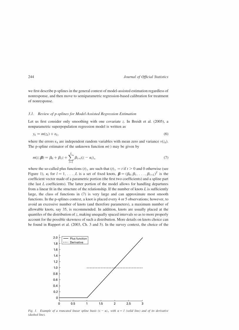
relationships and different combinations of such relationships. Firstly, values of a finite

population of N ¼ 5,000 units are generated for an auxiliary variable z from a uniform

[0,1] distribution. Then, six survey variables are obtained by using the following three

regression functions:

LIN : m{zÞ ¼ 0:8 þ 3z;

SIN : mðzÞ ¼ 1:8 þ 1:5zsin½4pðz2 0:6Þ�;

DIS :mðzÞ ¼ ð0:8 2 1:5zÞIðz , 0:25Þ þ ð0:8 þ 2zÞIð0:25 , z , 0:50Þ

þ ð21:7 þ 5zÞIð0:50 , z , 0:75Þ þ ð2:8 2 3zÞIðz . 0:75Þ:

Units are then randomly divided into two strata of equal dimension 2,500, to simulate

stratification on a variable different from z. Then, a constant value of 0.3 is added to m(z)

only for units in the first of the two strata. Then, the survey variables are constructed by

adding to m(zk) for k ¼ 1, : : : ,5,000 a heteroskedastic error component of the form

2ffiffiffiffiffiffiffiffizk1k

p, where 1k , N ð0;sÞ and s is set to 0.15 for a first set of three survey variables,

and to 0.50 for a second set.

Figure 2 shows the scatter plots of the six survey variables thus obtained. Grey crosses

and black circles distinguish units belonging to different strata. The LIN populations

(the first column) are considered as cases in which a calibration estimator that uses {1, z}

as auxiliary variables should provide a good protection against nonresponse bias. The SIN

populations (the second column) provide a situation in which the aforementioned vector of

auxiliary variables is not sufficiently adequate and for which gains in bias reduction are

expected from the proposed splines estimator. Finally, the DIS populations (the third

column) are generated under a discontinuous function of z, for which the spline estimator

is also based on a misspecified model.

Fig. 2. Scatter plot of the six survey variables versus the auxiliary variable. Variables in the first row have

errors with standard deviation 0.15, while those on the second row have errors with standard deviation 0.50.

Grey crosses and black circles denote units belonging to the two different strata.


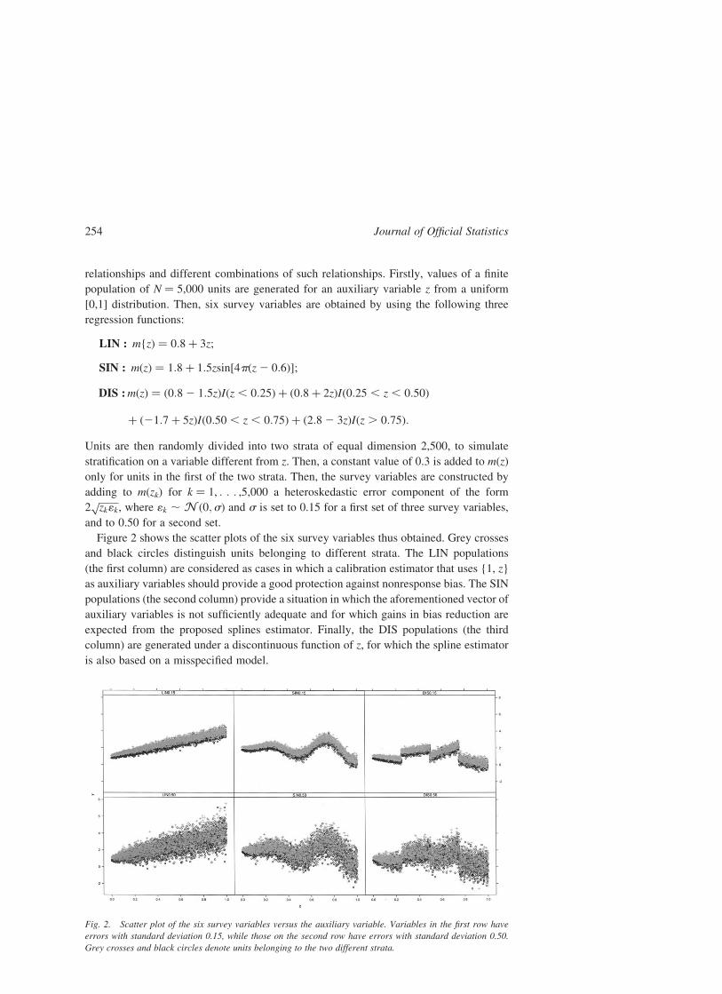
Each unit in the population has its own response probability attached. To study under

which circumstances the proposed estimator provides more protection against

nonresponse bias with respect to the classical calibration estimator, we will consider

different relationships between zk and uk. In particular, what is relevant here is the

relationship between zk and 1/uk as considered in Section 2 and 3.3. For this reason we

have considered the following four cases:

LIN : uk ¼ 1=ð1:2 þ zkÞ;

LOGþ : uk ¼ 0:3 þ 0:5=½1 þ exp ð6 2 15zkÞ�;

LOG2 : uk ¼ 0:3 þ 0:5=½1 þ exp ð26 þ 10zkÞ�;

GAU : uk ¼ 0:5= exp ½2ðzk 2 0:5Þ2=0:4�:

The response rate is approximately 60% in all cases. Figure 3 depicts these four sets of uks,

together with 1/uk. Different levels of complexity of the relationship between 1/uk and the

auxiliary variable allow to investigate in which situations the double protection property of

the calibration estimators holds with respect to the proposed spline estimator. For

example, the GAU case is inspired by the kernel of a Gaussian distribution and uk takes a

U-shape.

0.80.8

0.7

0.6

0.5

0.4

0.3

0.7

0.6

0.5

0.0 0.2 0.4 0.6 0.8 1.0 0.0 0.2 0.4 0.6 0.8 1.01.2

1.4

1.61/θ 1/θ

1/θ 1/θ

LIN LOG+

LOG– GAU

z z

z z

θ θθ

1.8

2.0

1.2

1.4

1.6

1.8

2.0

2.2

3.0

2.5

2.0

1.5

0.8

0.8

0.90.7

0.6

0.50.7

0.6

0.5

0.4

0.30.0 0.2 0.4 0.6 0.8 1.0 0.0 0.2 0.4 0.6 0.8 1.0

θ

3.0

2.5

2.0

1.5

Fig. 3. Scatter plot of the four sets of response probabilities versus the auxiliary variable (black). The dashed

line plots the inverse of the response probabilities versus z.


From each population, J ¼ 1,000 stratified random samples of dimensions n ¼ 250,

n ¼ 500 and n ¼ 800 have been selected. Disproportionate allocation is considered so that

40% of the sample comes from the first stratum and the remaining 60% comes from the

second. Recall that the first stratum is the one with the increased values. For all survey

variables this makes a 3 £ 4 design for the simulation – 3 sample sizes by 4 types of

response probabilities. For each unit in the sample, a Bernoulli experiment with

probability of success given by its response probability is conducted to simulate the

response mechanism.

On the response set the following estimators of the total of each survey variable have

been computed:

. exp ¼ N �yr, the expansion estimator where �yr ¼P

r dkyk=P

r dk, no auxiliary

information used;

. pwa ¼PP

p¼1Np �yrp population weighting adjustment, poststratified estimator

where P ¼ 3 poststrata are defined using the 0.33 and 0.66 quantiles of z

and �yrp ¼P

rpdkyk=

Prpdk, with rp the respondents set in poststratum p;

. wc ¼PP

p¼1Np �yrp weighting class estimator, poststratified estimator with estimated

population counts Np ¼P

spdk, with sp the sample set in poststratum p;

. ra ¼P

U zkP

r dkyk=P

r dkzk, the ratio estimator;

. reg ¼ exp þP

U zk 2 exp z

� �b, the regression estimator with exp z ¼

NP

r dkzk=P

r dk and b ¼P

r dkðzk 2 �zrÞð yk 2 �yrÞ=P

r dkðzk 2 �zrÞ2;

. reg2 ¼ exp þP

U zk 2 exp z

� �b1 þ

PU z2

k 2 exp z 2

� �b2, the quadratic regression

estimator;

. reg3 ¼ exp þP

U zk 2 exp z

� �b1 þ

PU z2

k 2 exp z 2

� �b2 þ

PU z3

k 2 exp z 3

� �b3,

the cubic regression estimator;

. sepra ¼PP

p¼1

PUp

zk �yrp=�zrp , the separate ratio estimator (the three poststrata in pwa

are used);

. sepreg ¼PP

p¼1Np �yrp þP

Upzk 2 �zrp

� �bp

n o, the separate regression estimator with

bp ¼P

rpdkðzk 2 �zrpÞð yk 2 �yrp Þ=

Prpdkðzk 2 �zrp Þ

2 (the three post-strata in pwa are

used);

. splinedf, eight different p-splines estimators according to the value of the degrees of

freedom used to approximate all survey variables; in particular, l is chosen so that

df ¼ {3,4,6,8,10,12,14,16}.

Estimators ra, reg, reg2, reg3, sepra, sepreg, and all the spline estimators are computed in

the estimators info-U and info-s scenario. For the latter case, an extra ‘s’ will be attached to

the name of the estimator. In addition, for the spline estimators the value of l has been

determined in two different ways for info-U and for info-s. In particular, for info-U l is

determined (i ) at the population level – using values of zk for k [ U – and kept fixed over

repeated sampling and (ii ) for each sample, at the response set level – using values of zkfor k [ r. Similarly, for info-s l is determined for each sample (i ) at the sample level –

using values of zk for k [ s – and (ii ) at the response set level – using values of zk for

k [ r. Estimators with l determined as in (ii) for either info-s or info-U will be denoted

with an extra ‘r’ in the name of the estimator. So, for example, spline4 denotes the

estimator that also uses 4 degrees of freedom, auxiliary information of type info-U and l

determined at the population level and then kept fixed over repeated sampling; while


spline4rs denotes the estimator that also uses 4 degrees of freedom, but auxiliary

information of type info-s and l computed at each replication at a response set level. The

spline-based estimators all use L ¼ 35 knots, placed at the quantiles of population values

of z and kept fixed over repeated sampling. Note that the choice of the position of the knots

is not as crucial as the choice of the position of thresholds for poststrata, once penalization

is included in the estimation procedure.

The performance of the estimators is evaluated for each survey variable using the

following measures in which Yj denotes the value taken by a generic estimator Y of Y at

replication j, with j ¼ 1; : : : ; J.

. % Relative Bias, given by

%RB ¼BðYÞ

Y100

where BðYÞ ¼ EðYÞ2 Y is the Monte Carlo estimate of the bias with

EðYÞ ¼ J21PJ

j¼1Yj;

. % Coefficient of Variation, given by

%CV ¼

ffiffiffiffiffiffiffiffiffiffi^MSE

pðYÞ

Y100

where the Monte Carlo estimate of the mean squared error is given by^MSEðYÞ ¼ J21

PJj¼1ðYj 2 YÞ2.

In addition, the performance of the variance estimators for the proposed estimator

illustrated in Theorem 3.2 has also been tested by means of the empirical coverage rate for

a 95% nominal confidence interval based on the normal approximation. Note that

estimators from exp to sepregs are “conventional” and also considered in Sarndal and

Lundstrom (2005). We will see that results are in line with those in for instance, Sarndal

and Lundstrom (2005, Sec. 10.3).

We will report results only for n ¼ 500 and then discuss the differences occurring when

considering a smaller or a larger sample size. Tables 1 and 2 report the % Relative Bias in

the different settings. Estimators that use info-U are displayed in the first half of the

tables. In general, it can be noted that for the same estimator, info-s shows the same

performance as info-U in terms of bias. Under the columns with the heading u LIN in

Table 1 we report results when the reciprocal of the nonresponse probabilities is a linear

function of the auxiliary variable. This is a situation in which condition (5) holds when the

auxiliary vector contains an intercept and the values of zk. This is the case for all reg

estimators – reg, reg2, reg3 – that, in fact, show an almost zero bias also for any population

of interest. This is also true for the sepreg and all the spline estimators even if they are using

a more complicated set of auxiliary variables than needed. Poststratification corresponds to

a piecewise constant approximation to the linear function that provides some reduction in

bias compared to exp, but not as well as the others. Estimators ra and sepra use an auxiliary

information vector which suffices approximate neither the nonresponse model nor the

population model, and in most cases show a larger bias than does exp.

When the inverse of the response probability is a more complicated function of z, as for

the case u LOGþ in Table 1 and u LOG2 and u GAU in Table 2, then the reg estimator


Table 1. Percent Relative Bias – %RB – for all estimators and survey variables. Response probabilities type LIN and LOGþ , n ¼ 500

u LIN uLOGþ

s ¼ 0.15 s ¼ 0.50 s ¼ 0.15 s ¼ 0.50

LIN SIN DIS LIN SIN DIS LIN SIN DIS LIN SIN DIS

exp 25.99 1.04 1.42 25.96 1.09 1.28 11.19 21.54 20.45 11.16 21.50 20.49pwa 20.70 0.53 0.77 20.66 0.65 0.71 0.98 0.23 0.43 0.97 0.17 0.41ra 4.27 12.17 12.60 4.31 12.23 12.45 26.02 216.74 215.80 26.05 216.70 215.83reg 20.02 0.05 0.15 0.03 0.13 0.11 20.02 0.98 8.58 20.18 1.01 8.35reg2 20.03 0.08 20.01 0.02 0.17 20.05 20.01 21.33 0.58 20.01 21.38 0.51reg3 20.03 0.06 20.08 0.02 0.15 20.13 20.02 21.82 0.33 0.00 21.89 0.27sepra 0.75 2.66 2.72 0.79 2.77 2.65 21.03 22.46 22.51 21.05 22.52 22.52sepreg 20.04 20.04 20.17 0.01 0.05 20.19 20.03 20.52 20.07 20.02 20.58 20.07spline3 20.03 0.07 0.08 0.02 0.16 0.04 20.02 20.08 4.21 20.09 20.09 4.07spline3r 20.03 0.07 0.04 0.02 0.15 0.00 20.02 20.36 2.98 20.07 20.39 2.86spline4 20.03 0.06 0.00 0.02 0.15 20.04 20.02 20.68 1.45 20.05 20.72 1.35spline4r 20.03 0.05 20.02 0.02 0.14 20.06 20.02 20.73 0.90 20.04 20.77 0.81spline6 20.04 0.01 20.05 0.01 0.10 20.08 20.02 20.51 0.27 20.04 20.55 0.20spline6r 20.04 20.01 20.05 0.01 0.08 20.09 20.02 20.38 0.17 20.05 20.41 0.10spline8 20.05 20.03 20.05 0.00 0.06 20.09 20.03 20.25 0.08 20.05 20.27 0.01spline8r 20.05 20.04 20.05 0.00 0.04 20.09 20.03 20.17 0.03 20.05 20.19 20.04spline10 20.05 20.05 20.06 0.00 0.03 20.09 20.03 20.14 0.00 20.05 20.16 20.07spline10r 20.06 20.05 20.06 20.01 0.02 20.09 20.04 20.12 20.04 20.06 20.13 20.12spline12 20.06 20.06 20.07 20.01 0.02 20.10 20.04 20.11 20.05 20.06 20.13 20.13spline12r 20.07 20.06 20.08 20.01 0.01 20.11 20.05 20.10 20.09 20.06 20.12 20.18spline14 20.07 20.07 20.08 20.01 0.01 20.11 20.05 20.10 20.10 20.06 20.12 20.18spline14r 20.07 20.07 20.10 20.02 0.00 20.14 20.06 20.10 20.14 20.07 20.12 20.22spline16 20.07 20.07 20.10 20.02 20.01 20.14 20.06 20.10 20.13 20.07 20.12 20.22spline16r 20.08 20.08 20.12 20.03 20.02 20.16 20.07 20.11 20.18 20.07 20.13 20.26

JournalofOfficia

lStatistics

25

8

Table 1. Continued

u LIN uLOGþ

s ¼ 0.15 s ¼ 0.50 s ¼ 0.15 s ¼ 0.50


wc 20.75 0.54 0.81 20.71 0.65 0.74 0.94 0.24 0.46 0.92 0.17 0.44ras 4.16 12.00 12.43 4.19 12.06 12.27 26.11 216.84 215.92 26.14 216.81 215.95regs 20.07 0.05 0.10 20.02 0.13 0.06 20.07 0.97 8.55 20.23 0.99 8.31reg2s 20.07 0.09 0.12 20.02 0.17 0.08 20.06 21.30 0.73 20.05 21.36 0.66reg3s 20.07 0.06 0.08 20.02 0.14 0.03 20.06 21.85 0.50 20.04 21.93 0.46sepras 0.71 2.66 2.74 0.75 2.77 2.67 21.08 22.47 22.49 21.10 22.53 22.50sepregs 20.08 0.03 0.05 20.02 0.11 0.02 20.07 20.46 0.16 20.06 20.52 0.16spline3s 20.07 0.07 0.12 20.02 0.15 0.08 20.06 20.08 4.25 20.14 20.11 4.10spline3rs 20.07 0.07 0.12 20.02 0.15 0.07 20.06 20.37 3.06 20.12 20.40 2.94spline4s 20.07 0.06 0.11 20.02 0.15 0.07 20.06 20.69 1.55 20.09 20.73 1.46spline4rs 20.07 0.06 0.11 20.02 0.14 0.07 20.06 20.73 1.02 20.08 20.77 0.95spline6s 20.08 0.03 0.10 20.03 0.11 0.06 20.06 20.49 0.42 20.08 20.53 0.36spline6rs 20.08 0.02 0.10 20.03 0.10 0.06 20.06 20.35 0.32 20.08 20.38 0.26splinc8s 20.08 0.01 0.10 20.03 0.09 0.06 20.06 20.20 0.24 20.08 20.23 0.18spline8rs 20.08 0.01 0.10 20.03 0.09 0.06 20.06 20.12 0.19 20.09 20.15 0.13spline10s 20.08 0.01 0.10 20.03 0.08 0.07 20.06 20.09 0.16 20.09 20.11 0.10spline10rs 20.08 0.00 0.10 20.04 0.08 0.07 20.07 20.06 0.13 20.09 20.08 0.06spline12s 20.08 0.00 0.11 20.04 0.08 0.07 20.07 20.05 0.11 20.09 20.07 0.05spline12rs 20.09 0.00 0.10 20.04 0.07 0.07 20.07 20.03 0.09 20.09 20.06 0.02spline14s 20.09 0.00 0.10 20.04 0.07 0.07 20.07 20.03 0.08 20.09 20.06 0.02spline14rs 20.09 0.00 0.10 20.04 0.06 0.06 20.08 20.03 0.06 20.09 20.06 0.00spline16s 20.09 0.00 0.10 20.04 0.06 0.06 20.08 20.03 0.06 20.09 20.06 0.00spline16rs 20.09 20.01 0.10 20.05 0.06 0.06 20.08 20.03 0.04 20.10 20.06 20.02

MontanariandRanalli:

Sem

iparametric

Regressio

nforNonresp

onse

Trea

tment

25

9

Table 2. Percent Relative Bias – %RB – for all estimators and survey variables. Response probabilities type LOG2 , and GAU, n ¼ 500

u LOG2 u GAU

s ¼ 0.15 s ¼ 0.50 s ¼ 0.15 s ¼ 0.50



JournalofOfficia

lStatistics

26

0

Table 2. Continued

u LOG2 u GAU

s ¼ 0.15 s ¼ 0.50 s ¼ 0.15 s ¼ 0.50


wc 21.11 1.32 3.10 21.08 1.41 3.11 20.04 23.02 23.76 0.07 23.02 23.85ras 8.06 22.07 28.78 8.07 22.03 28.57 20.13 22.39 28.21 0.04 22.39 28.20regs 20.10 20.76 5.96 20.10 20.75 5.91 20.03 22.07 27.84 0.14 22.07 27.84reg2s 20.09 21.23 0.30 20.01 21.23 0.30 20.05 0.30 20.06 20.04 0.38 20.17reg3s 20.09 21.06 0.44 20.02 21.07 0.42 20.05 0.24 20.09 20.04 0.32 20.20sepras 0.49 2.81 4.89 0.51 2.90 4.89 1.08 0.21 21.08 1.19 0.20 21.19sepregs 20.10 20.34 0.17 20.02 20.33 0.20 20.06 0.05 0.21 20.04 0.13 0.12spline3s 20.09 20.81 2.83 20.05 20.80 2.81 20.04 20.89 23.24 0.04 20.84 23.30spline3rs 20.09 20.81 2.01 20.04 20.80 1.99 20.05 20.68 22.44 0.02 20.63 22.51spline4s 20.09 20.74 0.96 20.03 20.73 0.94 20.05 20.28 20.89 20.01 20.21 20.97spline4rs 20.09 20.66 0.61 20.03 20.65 0.59 20.05 20.20 20.55 20.02 20.13 20.64spline6s 20.09 20.37 0.24 20.04 20.35 0.22 20.06 20.06 20.04 20.04 0.02 20.13spline6rs 20.09 20.26 0.20 20.04 20.24 0.17 20.06 20.04 0.02 20.04 0.03 20.08spline8s 20.09 20.15 0.18 20.05 20.13 0.15 20.06 20.03 0.07 20.04 0.05 20.02spline8rs 20.09 20.10 0.17 20.06 20.08 0.14 20.06 20.02 0.09 20.04 0.05 0.00spline10s 20.10 20.08 0.17 20.06 20.06 0.13 20.06 20.02 0.10 20.04 0.06 0.01spline10rs 20.10 20.06 0.17 20.07 20.04 0.13 20.06 20.02 0.10 20.04 0.06 0.01spline12s 20.10 20.05 0.16 20.07 20.03 0.12 20.07 20.02 0.10 20.04 0.06 0.01spline12rs 20.10 20.04 0.16 20.08 20.02 0.11 20.07 20.02 0.10 20.04 0.05 0.01spline14s 20.10 20.04 0.16 20.08 20.02 0.11 20.07 20.02 0.10 20.04 0.05 0.01spline14rs 20.11 20.04 0.15 20.09 20.02 0.10 20.07 20.03 0.10 20.04 0.05 0.01spline16s 20.11 20.04 0.15 20.09 20.02 0.10 20.07 20.03 0.10 20.04 0.05 0.01spline16rs 20.11 20.04 0.14 20.09 20.02 0.09 20.07 20.03 0.10 20.05 0.05 0.00


Sem

iparametric

Regressio

nforNonresp

onse

Trea

tment

26

1

successfully reduces bias to almost zero only with a LIN population. For the other

populations, reg always suffers from a misspecified response or population model.

By contrast, reg2 and reg3, that use, respectively, a quadratic and a cubic model for either

the relationship between y and z or between 1/u and z, allow the reduction of nonresponse

bias also in the case of the SIN or DIS populations, when the response probabilities are of

type GAU. Note that for info-U reg2 requires the knowledge of the population total of z 2,

and reg3 further requires also the population total of z 3. Estimator sepreg succeeds in

decreasing bias every time a piecewise linear approximation in each poststratum provides

a good description of the relationship between y and z – for instance the DIS cases – or

between 1/u and z – for instance the GAU cases.

On the other hand, the spline estimators almost always succeed in taking the bias to zero

because the inclusion of the basis functions allow handling departures from linearity in

either the response model or the population model. Note, for instance, that the DIS

population is based on a function of z that the spline estimators cannot handle because the

function is discontinuous. In these cases also, though, bias is reduced because the implicit

estimation of the inverse of the response probabilities allows to handle the LOG and the

GAU functions.

The ability of the spline estimators to capture either the response model or the population

model depends on the penalty l and, therefore, on the number of degrees of freedom used.

The simulation studies show that it is better to have a relatively larger value for the degrees

of freedom: this allows the handling of even complicated structures, like the SIN population

or the LOG response models, and does not provide significant losses when in the presence

of simple linear structures. In addition, it is hard to detect differences in the performance of

the alternative spline estimators, once at least 8 degrees of freedom are used.

Tables 3 and 4 report %CV for the simulations. In these tables, as expected, the

difference between info-s and info-U versions of the same estimator are more clear, with

the latter providing gains in efficiency over the former when the vector of auxiliary

variables employed by the estimator provides a good approximation of the population

model. It is the case of reg in the LIN populations, and of spline estimators for LIN and

SIN populations. Estimator sepreg, that showed a good performance in decreasing bias,

suffers from its coarse approximation of functions like the SIN or the LOG and GAU, by a

relatively larger overall error.

As for the role of l for the spline estimators, again here there is very little difference in

performance among estimators with a number of degrees of freedom going from 8 to 16. In

addition, virtually no difference can be detected for each spline estimator with a given

number of degrees of freedom when l is chosen at the population (sample) level on the one

hand or at a response set level on the other. This provides evidence of little increase in

variability due to the estimation of its value at a response set level (see Section 3.4).

In general, simulations with a larger (smaller) sample size show, other things being

equal, an increase (decrease) in the role of bias as opposed to that of variance. The spline

estimators, as all nonparametric regression techniques, suffer from a reduced number of

observations and therefore provide better performances both in terms of %RB and %CV

when n ¼ 800.

As for the performance of the variance estimators for the proposed estimators, Tables 5

and 6 report coverage rates for 95% confidence intervals for all spline estimators.


Table 3. % Coefficient of variation for all estimators and survey variables. Response probabilities type LIN and LOGþ , n ¼ 500

u LIN u LOGþ

s ¼ 0.15 s ¼ 0.50 s ¼ 0.15 s ¼ 0.50




Sem

iparametric

Regressio

nforNonresp

onse

Trea

tment

26

3

Table 3. Continued

u LIN u LOGþ

s ¼ 0.15 s ¼ 0.50 s ¼ 0.15 s ¼ 0.50



JournalofOfficia

lStatistics

26

4

Table 4. % Coefficient of variation for all estimators and survey variables. Response probabilities type LOG2 and GAU, n ¼ 500

u LOG2 u GAU

s ¼ 0.15 s ¼ 0.50 s ¼ 0.15 s ¼ 0.50




Sem

iparametric

Regressio

nforNonresp

onse

Trea

tment

26

5

Table 4. Continued

u LOG2 u GAU

s ¼ 0.15 s ¼ 0.50 s ¼ 0.15 s ¼ 0.50



JournalofOfficia

lStatistics

26

6

Table 5. Coverage rate for 95% confidence intervals for all p-splines based estimators and survey variables. Response probabilities type LIN and LOGþ , n ¼ 500

u LIN u LOGþ

s ¼ 0.15 s ¼ 0.50 s ¼ 0.15 s ¼ 0.50


spline3 94.6 93.8 95.3 95.4 94.0 95.6 95.3 96.1 62.9 94.7 95.1 85.6spline3r 94.6 93.9 95.0 95.4 93.8 95.6 95.1 95.4 74.6 94.5 94.6 90.1spline4 94.6 94.6 94.8 95.1 93.9 95.5 94.8 94.2 89.7 94.3 93.8 93.6spline4r 94.4 94.6 95.0 95.1 94.1 95.5 94.8 92.7 92.9 94.3 93.6 95.0spline6 94.0 95.3 95.1 94.5 94.4 95.3 94.9 93.2 94.9 94.3 93.4 95.0spline6r 93.9 95.2 95.1 94.4 94.3 95.1 94.8 94.7 94.5 94.3 93.5 95.2spline8 93.9 95.5 94.0 94.0 94.1 95.1 94.5 95.3 94.9 94.3 93.4 95.2spline8r 94.0 95.1 93.6 94.0 94.1 94.7 94.3 95.1 94.6 94.2 94.1 95.1spline10 94.0 94.8 93.7 93.8 94.0 94.3 94.3 94.9 94.7 94.2 94.0 95.4spline10r 93.5 95.1 93.9 93.6 93.9 94.3 94.2 95.0 94.5 94.2 93.8 95.8spline12 93.4 94.6 93.7 93.6 93.6 94.4 94.2 95.1 94.5 94.2 93.9 95.7spline12r 93.5 94.5 93.1 93.3 93.7 94.1 94.0 95.0 94.7 93.9 93.8 95.7spline14 93.4 94.4 92.8 93.3 93.6 94.1 94.0 94.8 94.7 93.8 93.8 95.7spline14r 93.3 93.8 92.4 93.0 93.6 94.1 93.6 95.0 94.8 93.4 93.6 95.5spline16 93.3 93.8 92.4 93.0 93.6 94.1 93.7 95.0 94.8 93.4 93.6 95.5spline16r 93.4 93.4 92.2 92.9 93.4 94. lj 93.5 94.6 94.2 93.4 93.1 95.2


Sem

iparametric

Regressio

nforNonresp

onse

Trea

tment

26

7

Table 5. Continued

u LIN u LOGþ

s ¼ 0.15 s ¼ 0.50 s ¼ 0.15 s ¼ 0.50


spline3s 94.9 94.8 95.4 94.6 94.3 95.5 94.8 96.1 70.8 94.0 95.1 86.6spline3rs 95.0 95.2 95.3 94.6 94.3 95.6 95.0 95.8 81.4 93.8 94.7 91.0spline4s 95.0 94.6 95.2 94.6 94.2 95.5 95.2 94.9 90.8 94.0 94.4 94.2spline4rs 95.0 94.5 94.8 94.6 93.9 95.4 95.4 94.7 92.9 94.0 94.3 95.4spline6s 95.0 94.7 94.7 94.7 94.1 95.7 95.4 94.8 94.7 94.1 94.5 95.7spline6rs 95.0 94.7 94.7 94.8 94.3 95.7 95.4 95.1 94.9 94.1 94.8 95.8spline8s 95.0 95.0 94.2 94.8 94.3 95.6 95.3 95.4 94.8 94.1 94.5 95.7spline8rs 95.0 95.3 94.3 94.8 94.3 95.4 95.4 95.1 94.6 94.0 94.9 95.9spline10s 95.0 95.1 94.5 94.8 94.2 95.2 95.4 94.9 94.6 94.0 94.8 95.9spline10rs 95.0 95.2 94.7 94.7 94.3 94.8 95.5 94.9 94.6 94.0 95.0 96.0spline12s 95.0 95.2 94.6 94.7 94.4 94.9 95.5 94.9 94.8 94.0 95.0 96.2spline12rs 94.9 95.3 94.6 94.7 94.5 94.7 95.5 95.0 94.7 94.1 95.2 96.3spline14s 94.9 95.4 94.7 94.7 94.5 94.8 95.5 95.0 94.8 94.2 95.2 96.3spline14rs 94.9 95.5 94.7 94.7 94.5 94.8 95.5 95.0 94.8 94.0 95.3 96.4spline16s 94.9 95.5 94.7 94.7 94.4 94.8 95.5 95.0 94.8 94.0 95.3 96.4spline16rs 94.9 95.5 95.1 94.6 94.5 94.7 95.6 95.2 94.9 94.1 95.1 96.4

JournalofOfficia

lStatistics

26

8

Table 6. Coverage rate for 95% confidence intervals for all p-splines based estimators and survey variables. Response probabilities type LOG2 and GAU; n ¼ 500

u LOG2 u GAU

s ¼ 0.15 s ¼ 0.50 s ¼ 0.15 s ¼ 0.50


spline3 94.0 92.5 86.6 94.5 93.7 91.8 94.5 91.2 71.8 94.2 93.1 87.3spline3r 94.0 92.2 90.3 94.4 93.5 93.5 94.5 92.3 81.9 94.1 94.0 90.8spline4 93.8 92.2 93.4 94.3 93.8 94.9 94.4 94.4 93.2 94.1 94.1 95.0spline4r 93.9 92.9 94.0 94.2 93.7 94.8 94.3 95.7 94.7 94.2 94.0 95.5spline6 93.3 94.1 94.4 94.2 93.2 94.9 93.9 94.9 94.7 93.9 94.0 96.1spline6r 93.3 94.9 94.4 94.2 93.5 94.7 93.9 94.5 94.6 94.0 94.4 96.3spline8 93.2 94.4 94.2 93.9 93.5 94.5 94.0 93.8 94.3 93.9 94.3 95.9spline8r 93.0 94.4 94.5 93.8 93.7 94.4 93.9 93.7 93.9 93.8 94.4 95.7spline10 92.6 94.0 94.9 93.8 93.9 94.5 93.9 92.7 93.7 93.8 94.3 95.5spline10r 92.8 94.3 94.5 93.7 94.0 94.7 93.7 92.7 93.2 93.8 94.1 95.3spline12 92.6 94.2 94.2 93.2 93.9 94.6 93.5 92.8 93.3 93.8 94.0 95.4spline12r 92.1 93.9 94.0 92.8 93.6 94.3 93.2 92.9 93.4 93.8 93.8 95.5spline14 92.1 93.9 93.8 92.8 93.6 94.3 93.1 92.9 93.6 93.9 93.6 95.5spline14r 91.8 93.7 93.5 92.6 93.0 94.2 93.0 92.7 94.0 93.7 93.3 95.4spline16 91.9 93.7 93.6 92.6 93.0 94.2 93.0 92.5 94.0 93.7 93.3 95.4spline16r 91.5 93.8 93.1 92.6 92.4 93.8 92.7 92.5 93.9 93.5 93.4 95.7


Sem

iparametric

Regressio

nforNonresp

onse

Trea

tment

26

9

Table 6. Continued

u LOG2 u GAU

s ¼ 0.15 s ¼ 0.50 s ¼ 0.15 s ¼ 0.50


spline3s 94.9 93.0 87.4 95.3 93.7 91.6 95.8 92.2 82.4 96.0 93.3 89.5spline3rs 95.1 93.0 91.9 95.3 93.3 94.1 95.8 93.2 88.0 96.0 93.9 91.9spline4s 95.3 93.1 94.3 95.2 93.3 95.6 95.5 94.2 95.1 95.8 94.5 95.1spline4rs 95.3 93.3 94.3 95.4 93.6 95.3 95.4 94.2 95.5 95.7 94.5 95.6spline6s 95.5 94.7 94.3 95.4 94.1 95.4 95.2 94.7 95.3 95.9 95.2 95.9spline6rs 95.5 95.3 94.4 95.3 94.3 95.4 95.1 94.8 95.2 95.9 95.0 95.9spline8s 95.4 95.2 94.3 95.2 94.5 95.5 95.1 94.8 95.0 95.9 95.2 96.1spline8rs 95.3 95.1 94.6 95.0 94.7 95.3 95.1 94.9 94.9 95.8 95.2 96.1spline10s 95.3 94.9 94.8 95.0 95.0 95.3 95.1 95.0 94.6 95.8 95.1 96.2spline10rs 95.3 94.6 94.7 95.0 95.0 95.1 95.1 95.2 94.4 95.7 95.0 96.3spline12s 95.3 94.6 94.6 94.9 95.0 95.2 95.1 95.2 94.4 95.7 94.9 96.2spline12rs 95.4 94.6 94.9 94.9 94.9 94.9 95.1 95.2 94.5 95.7 95.0 96.3spline14s 95.4 94.6 94.8 94.9 94.9 94.9 95.2 95.2 94.5 95.7 95.1 96.2spline14rs 95.4 94.6 95.1 94.8 94.8 94.7 95.2 95.2 94.2 95.7 95.1 96.1spline16s 95.4 94.6 95.1 94.8 94.8 94.7 95.2 95.2 94.2 95.7 95.1 96.1spline16rs 95.4 94.6 95.1 94.9 94.6 94.6 95.1 95.2 94.3 95.7 94.9 96.2

JournalofOfficia

lStatistics

27

0

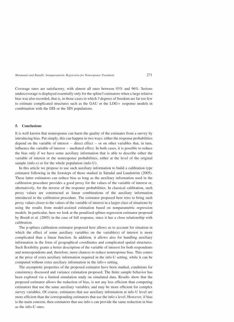
Coverage rates are satisfactory, with almost all rates between 93% and 96%. Serious

undercoverage is displayed essentially only for the spline3 estimators when a large relative

bias was also recorded, that is, in those cases in which 3 degrees of freedom are far too few

to estimate complicated structures such as the GAU or the LOGþ response models in

combination with the DIS or the SIN populations.

5. Conclusions

It is well known that nonresponse can harm the quality of the estimates from a survey by

introducing bias. Put simply, this can happen in two ways: either the response probabilities

depend on the variable of interest – direct effect – or on other variables that, in turn,

influence the variable of interest – mediated effect. In both cases, it is possible to reduce

the bias only if we have some auxiliary information that is able to describe either the

variable of interest or the nonresponse probabilities, either at the level of the original

sample (info-s) or for the whole population (info-U).

In this article we propose to use such auxiliary information to build a calibration type

estimator following in the footsteps of those studied in Sarndal and Lundstrom (2005).

These latter estimators can reduce bias as long as the auxiliary information used in the

calibration procedure provides a good proxy for the values of the variable of interest or,

alternatively, for the inverse of the response probabilities. In classical calibration, such

proxy values are constructed as linear combinations of the auxiliary information

introduced in the calibration procedure. The estimator proposed here tries to bring such

proxy values closer to the values of the variable of interest in a larger class of situations by

using the results from model-assisted estimation based on nonparametric regression

models. In particular, here we look at the penalized splines regression estimator proposed

by Breidt et al. (2005) in the case of full response, since it has a close relationship with

calibration.

The p-splines calibration estimator proposed here allows us to account for situation in

which the effect of some auxiliary variables on the variable(s) of interest is more

complicated than a linear function. In addition, it allows also for handling auxiliary

information in the form of geographical coordinates and complicated spatial structures.

Such flexibility grants a better description of the variable of interest for both respondents

and nonrespondents and, therefore, more chances to reduce nonresponse bias. This comes

at the price of extra auxiliary information required in the info-U setting, while it can be

computed without extra auxiliary information in the info-s setting.

The asymptotic properties of the proposed estimator have been studied, conditions for

consistency discussed and variance estimation proposed. The finite sample behavior has

been explored via a limited simulation study on simulated data. Results show that the

proposed estimator allows the reduction of bias, is not any less efficient than competing

estimators that use the same auxiliary variables, and may be more efficient for complex

survey variables. Of course, estimators that use auxiliary information at info-U level are

more efficient than the corresponding estimators that use the info-s level. However, if bias

is the main concern, then estimators that use info-s can provide the same reduction in bias

as the info-U ones.


Like all nonparametric regression-based estimators, the performance of the proposed

estimator depends on the selection of a smoothing parameter that governs its

approximation ability. However, note that in the survey context, trying to find the

optimal parameter is not as relevant as in the standard context: the estimator is not

constructed for a single variable, but for a large set of variables collected during the

survey. A penalty that is optimal for one variable may well not be adequate for another, but

using different sets of weights would not be feasible for coherence issues. We have

therefore considered a single fixed value for it and given some guidelines to selecting its

value. In this regard, Sarndal and Lundstrom (2008) have proposed an indicator that allows

the ranking of different auxiliary vectors for their potential to reduce the bias for the

calibration estimator. It will be interesting to investigate how this indicator can be

modified to encompass penalized calibration (and hence p-splines) by comparing the use

of a continuous auxiliary variable as it stands (linear), with dividing it into different groups

or poststrata (piecewise linear), and with p-splines (nonparametrical).

A. Proofs

Proof of Theorem 3.1. First note that for info-U Yp;r ¼P

U zTk br, with

br ¼r

Xdkzkz

Tk þLN

!21

r

Xdkzkyk; ðA:1Þ

becauser

Pdk yk 2 zTk br

� �¼ 0 for the properties of GLS estimators and noting that the first

element of br remains unpenalized. Therefore, Yp;r 2 Y ¼P

U zTk ðbr 2 gUÞ2P

U ek,

where ek ¼ yk 2 zTkgU . For info-s Yp;r ¼P

s dkzTk br and

Yp;r 2 Y ¼U

XzTk ðbr 2 gUÞ þ

s

Xdkzk 2

U

Xzk

0@

1AT

gU

þs

Xdkzk 2

U

Xzk

0@

1AT

ðbr 2 gUÞ2U

Xek ðA:2Þ

Note that gU is such that

gU ¼U

Xukzkz

Tk þLN

0@

1A21

U

Xukzkek þ

U

Xukzkz

TkgU þLNgU 2LNgU

24

35

¼ gU þU

Xukzkz

Tk þLN

0@

1A

21

U

Xukzkek 2LNgU

24

35:


This implies thatU

Pukzkek ¼ LNgU . Now,

br 2 gU ¼r

Xdkzkz

Tk þLN

!21

r

Xdkzkyk 2 gU

¼r

Xdkzkz

Tk þLN

!21

r

Xdkzkyk 2

r

Xdkzkz

Tk þLN

!gU

" #

¼r

Xdkzkz

Tk þLN

!21

r

Xdkzkek þ

r

Xdkzkz

TkgU 2

r

Xdkzkz

TkgU 2LNgU

" #

¼r

Xdkzkz

Tk þLN

!21"r

Xdkzkek 2

U

Xukzkek:

#

The conditional expectation of the components of br in (A.1) is given by

Er

Xdkzkz

Tk jFN

( )¼

U

Xukzkz

Tk and E

r

XdkzkykjFN

( )¼

U

Xukzkyk

Then, by Assumption A2 it follows that br 2 gU ¼ Op n21=2N

� �because

N21P

r dkzkzTk þLN

� �is bounded by bounding arguments on z and Assumptions A3

and A4. In addition, given thatP

U ukzkek ¼ LNgU by the first part of assumption A5,

for which there exists a vector d such that zTk d ¼ ~zTk d1 þ z*Tk d2 ¼ u21

k , with ~zk ¼ ð1; zkÞT

and z*k ¼ ððzk 2 k1Þþ; : : : ; ðzk 2 kLÞþÞ

T , then we can writeP

U ek ¼ dTLNgU ¼

0; 0; lNdT2

� �gU ¼ O Nn21

N

� �The last equality follows from the second part of

Assumption A5.

To obtain representation (11) we follow Fuller (2009, Ch. 5). Assume, without loss of

generality, that the first element of z is u21k . In fact, because of A5, u21

k is in the space

spanned by the columns of Z r and we can transform the matrix of values of zk so that the

first element is the inverse of uk. In particular, consider the following transformation of the

vector z by zk ¼ Qzk with

z1k ¼ u21k

zlk ¼ zlk þ z1kq1l

where

q1l ¼ 2r

Xdkz

21k

!21

r

Xdkz1kzlk;

for l ¼ 2; 3; : : : ; Lþ 2 and Q ¼ diag{1; q1l}l¼2; : : : ;Lþ2. Now, for info-U,

Yp;r 2 Y ¼P

U zTk ðbr 2 gUÞ þP

U ek ¼P

U zTk Q21ðbr 2 gUÞ þ O Nn21

N

� �. Note that

XU

zTk ¼U

Xz1k; 0; : : : ; 0

0@

1Aþ Op Nn

21=2N

� �


because of A1, A2 and A4. Now

Q21ðbr 2 gUÞ ¼r

Xdkzkz

Tk þ QLNQÞ

21

!r

Xdkzkek þ QLNgU

!;

whose first element is such that

r

Xdkz

21k

!21

r

Xdkz1kek ¼

U

Xz1k

0@

1A

21

r

Xdkz1kek þ Op Nn21

N

� �;

so that (11) is obtained. Finally, (12) can be obtained for info-s from (A.2). The ek (and the

zTkgU for info-s) have bounded fourth moments by the moment assumptions so that, by

assumption A2, N21 ffiffiffiffiffiffinN

pðYp;r 2 YÞjFN has a normal distribution in the limit. The form of

the variance in (14) follows from (11), while (15) can be obtained from

Vr

X ek

p2k

2s

X ek

pk

þs

X yk

pk

jFN

!¼ VpðsÞ E

r

X ek

p2k

2s

X ek

pk

þs

X yk

pk

js

!" #

þ EpðsÞ Vs

X ek

p2k

js

!" #¼ VpðsÞ

s

X yk

pk

" #þ EpðsÞ

s

X e2k

p22k

ukð1 2 ukÞ

" #; ðA:3Þ

where subscript p(s) denotes expectation and variance taken with respect to the sampling

design. B

Proof of Theorem 3.2. First note that by using conditional arguments as in (A.3),

variances in (14) and in (15) can be rewritten as

V1ðYp;rÞ ¼ VpðsÞs

X ek

pk

" #þ EpðsÞ V

r

X ek

p2k

js

!" #; for info–U

V1ðYp;rÞ ¼ VpðsÞs

X yk

pk

" #þ EpðsÞ V

r

X ek

p2k

js

!" #; for info–s:

The expectation of the following Horvitz-Thompson variance estimator forP

r wkek is


given by

Er

Xr

Xpkj 2 pkpkj

pkj

wkekwjejjFN

( )

¼U

Xpk 2 p2

k

� �ukw

2ke

2k þ

Uk–j

XU

Xðpkj 2 pkpkjÞukujwkekwjej

¼U

Xpk 2 p2

k

� �ukw

2ke

2k þ

U

XU

Xðpkj 2 pkpkjÞukujwkekwjej

2U

Xpkuk 2 p2

ku2k

� �w2ke

2k

¼U

XU

Xðp2kj 2 p2kp2jÞwkekwjej 2

U

Xðpk 2 p2kÞp2kw

2ke

2k :

By A7 and given that br 2 gU ¼ Op n21=2N

� �the variance estimator constructed using ek

is asymptotically equivalent to the one that uses ek, and the result is proven. B

6. References

Beaumont, J.F. and Bocci, C. (2008). Another Look at Ridge Calibration. Metron, 66,

5–20.

Breidt, F.J., Claeskens, G., and Opsomer, J.D. (2005). Model-Assisted Estimation for

Complex Surveys Using Penalised Splines. Biometrika, 92, 831–846.

Deville, J.-C. (2000). Generalized Calibration and Application to Weighting for

Non-Response. J. G. a. Bethlehem and P. G. M. a. van der Heijden (Eds), COMPSTAT –

Proceedings in Computational Statistics, 14th Symposium, 65–76. Physica-Verlag

Ges.m.b.H.

Deville, J.-C. and Sarndal, C.-E. (1992). Calibration Estimators in Survey Sampling.

Journal of the American Statistical Association, 87, 376–382.

Eilers, P.H.C. and Marx, B.D. (1996). Flexible Smoothing with B-splines and Penalties.

Statistical Science, 11, 89–121.

Ekholm, A. and Laaksonen, S. (1991). Weighting via Response Modeling in the Finnish

Household Budget Survey. Journal of Official Statistics, 7, 325–337.

Folsom, R.E. (1991). Exponential and Logistic Weight Adjustments for Sampling and

Nonresponse Error Reduction. ASA Proceedings of the Social Statistics Section,

197–202.

Fuller, W.A. (2002). Regression Estimation for Survey Samples. Survey Methodology, 28,

5–25.

Fuller, W.A. (2009). Sampling Statistics. Hoboken, NJ: Wiley, Wiley Series in Survey

Methodology.

Fuller, W.A. and An, A.B. (1998). Regression Adjustments for Nonresponse. Journal of

the Indian Society of Agricultural Statistics, 51, 331–342.


Fuller, W.A., Loughin, M.M., and Baker, H.D. (1994). Regression Weighting in the

Presence of Nonresponse with Application to the 1987–1988 Nationwide Food

Consumption Survey. Survey Methodology, 20, 75–85.

Giommi, A. (1987). Nonparametric Methods for Estimating Individual Response

Probabilities. Survey Methodology, 13, 127–134.

Guggemos, F. and Tille, Y. (2010). Penalized Calibration in Survey Sampling: Design-

based Estimation Assisted by Mixed Models. Journal of Statistical Planning and

Inference, 140, 3199–3212.

Isaki, C.T. and Fuller, W.A. (1982). Survey Design under the Regression Superpopulation

Model. Journal of the American Statistical Association, 77, 89–96.

Kim, J.K. and Kim, J.J. (2007). Weighting Adjustment using Estimated Response

Probability. The Canadian Journal of Statistics/La Revue Canadienne de Statistique, 35,

501–514.

Kott, P.S. (2006). Using Calibration Weighting to Adjust for Nonresponse and Coverage

Errors. Survey Methodology, 32, 133–142.

Little, R.J.A. (1986). Survey Nonresponse Adjustments for Estimates of Means.

International Statistical Review, 54, 139–157.

Lundstrom, S. and Sarndal, C.E. (1999). Calibration as a Standard Method for Treatment

of Nonresponse. Journal of Official Statistics, 15, 305–327.

Montanari, G.E. and Rananlli, M.G. (2005). Nonparametric Model Calibration

Estimation in Survey Sampling. Journal of the American Statistical Association,

100, 1429–1442.

Park, M. and Fuller, W.A. (2009). The Mixed Model for Survey Regression Estimation.

Journal of Statistical Planning and Inference, 139, 1320–1331.

Rao, J.N.K. and Singh, A.C. (1997). A Ridge-Shrinkage Method for Range Restricted

Weight Calibration in Survey Sampling. In Proceedings of the American Statistical

Association, Section on Survey Research Methods, 57–65.

Ruppert, D. (2002). Selecting the Number of Knots for Penalized Splines. Journal of

Computational and Graphical Statistics, 11, 735–757.

Ruppert, D., Wand, M.P., and Carrol, R. (2003). Semiparametric Regression. Cambridge,

New York: Cambridge University Press.

Sanchez-Borrego, I., Opsomer, J. D., Rueda, M., and Arcos A. (2011). Nonparametric

Regression with Mixed Data Types in Survey Sampling. Preprint submitted to Revista

Matematica Complutense.

Sarndal, C.-E. (2007). The Calibration Approach in Survey Theory and Practice. Survey

Methodology, 33, 99–119.

Sarndal, C.-E. and Lundstrom, S. (2005). Estimation in Surveys with Nonresponse. Wiley:

Chichester.

Sarndal, C.-E. and Lundstrom, S. (2008). Assessing Auxiliary Vectors for Control of

Nonresponse Bias in the Calibration Estimator. Journal of Official Statistics, 24, 167–191.

Sarndal, C.-E., Swensson, B. and Wretman, J. (1992). Model Assisted Survey Sampling.

Berlin, New York: Springer.

Silva, D.N.D. and Opsomer, J.D. (2006). A Kernel Smoothing Method of Adjusting for

Unit Non-response in Sample Surveys. The Canadian Journal of Statistics/La Revue

Canadienne de Statistique, 34, 563–579.


Wu, C. and Sitter, R.R. (2001). A Model-Calibration to Using Complete Auxiliary

Information from Survey data. Journal of the American Statistical Association, 96,

185–193.

Received November 2009

Revised January 2012


calibration inspired by semiparametric regression as a ... · calibration inspired by...

Documents