caliste and its applications
TRANSCRIPT

1 CEA Saclay IRFU/DAp, 2 CEA Saclay IRFU/DEDIP,3 CEA Saclay LIST/LCAE, 4 3D plus
SEPT, 26th 2017, CEA, Saclay, France
CALISTE and its applications
Daniel Maier1, P.A. Bausson2, C. Blondel1, F. Carrel3,
G. Daniel1, C. Force3, O. Gevin2, H. Lemaire3,
O. Limousin1, D. Renaud1, J. Martignac1, A. Meuris1,
V. Schoepff3, F. Soufflet4, M.C. Vassal4, F. Visticot1

SUMMARY
Daniel Maier | SEPT 2017 | PAGE 2
ORIGAMIX: a portable
X- and gamma-ray
spectro-imaging camera
fields of application
history of the project
physical concepts
actual status
next steps
SATBOT: realtime
dosimetry
for radiotherapy
NP + radiotherapy
XRF dosimetry
physical concepts
actual status
next steps
CALISTE: a compact
X-ray spectro-imager
module
history
IDeF-X family
CALISTE family

PROJECT HISTORY
Daniel Maier | SEPT 2017 | PAGE 3
CALISTE is based on a long line of experience
but also aims for challenging new developments
based on IDeF-X readout ASICs- started in 2003; now in 7th generation
- properties: ultra-low noise, low power consumption,
channel individual triggered readout
integrated into a CALISTE module- combining several ASICs
- 3D electronics by 3D+
different combinations of ASICs + housing
CALISTE-64 CALISTE-256 CALISTE-HD CALISTE-SO D2R1 CALISTE-HD-BD
2007 2009 2011 2013 2016
more pixel less power better spec. & spat. resolution larger energy range
64 → 256 200mW→200mW 900μm → 300μm 250 keV → 1 MeV
900 eV → 580 eV FWHM @ 60keV

PROJECT HISTORY
ORIGAMIX uses a CALISTE module (HD or O) and
builds a portable device
a portable device
stable & safe housing
ensure vacuum tightness
cooling?
compact, low-power electronics
power supply: batteries, HV?
softwarereliability
easy to use and to understand → alert
control of
operation
user-friendly
mostly autonomous
parameters
calibration
analysis
0.5 mm Al
entrance
window
CALISTE HD
2x TEC modules
Flex PCB connexion
Carrier
motherboard
Power
management
Eth
Zynq SoCMicroZed
Interface board
CALISTE SC & DAQ
Wix
HV crystal bias
House keepingHV cable Daniel Maier | SEPT 2017 | PAGE 4
design:

CURRENT STATUS
Daniel Maier | SEPT 2017 | PAGE 5
detector: Caliste-HD
10 x 10 x 1 mm³ CdTe
camera: system-on-chip aq. system
thermo-electrical coolers
dimension: 7.5 x 7.5 x 23 cm³
mass: m < 1 kg
power: p < 10 W

TYPICAL FIELDS OF APPLICATION
Daniel Maier | SEPT 2017 | PAGE 6
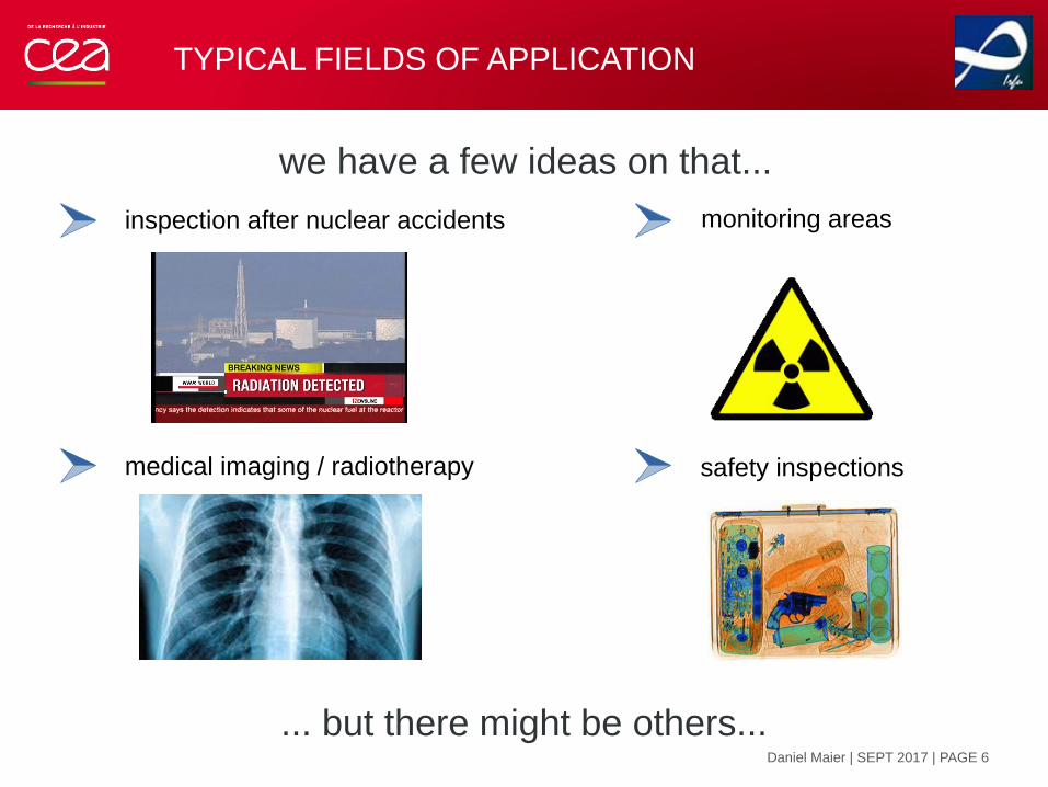
we have a few ideas on that...
inspection after nuclear accidents
TYPICAL FIELDS OF APPLICATION
Daniel Maier | SEPT 2017 | PAGE 6
we have a few ideas on that...
monitoring areasinspection after nuclear accidents
medical imaging / radiotherapy safety inspections
... but there might be others...

PHYSICAL CONCEPTS
Daniel Maier | SEPT 2017 | PAGE 7
CdTe is becomming inefficient for E > 100-300 keV.
Then, Compton scattering gets the dominant effect.
photon interactions detection efficiency
photon interaction with CdTe (ZCd = 48, ZTe = 52)
1 10 100 1000 10 000
coherent scattering (a)incoherent scattering (b)
photoelectirc absorption (c)nuclear pair production (d)
electronic pair production (e)total ( f )
photon energy E [keV]
cro
ss s
ectio
n [b
arn
/ato
m]
10-4
10-3
10-2
10-1
100
101
102
103
104
105
(a)
(b)(c)
(f)
(d)
(e)
1
10
100
10 100 1000
photon energy E [keV]
inte
ractio
n p
rob
ab
ility
[%
]
d = 0.5 mm
d = 1.0 mm
d = 2.0 mm
d = 3.0 mm
d = 5.0 mm
P.E. only
P.E. + I.S.
CdTe
= photo electric absorption
= incoherent scattering ("Compton")
P.E.
I.S.
50 500
5
50

PHYSICAL CONCEPTS
Daniel Maier | SEPT 2017 | PAGE 8
IMAGING = source location
most promising is a two fold approach: mask + Compton
coded mask
+ high spatial resolution
+ big field-of-view
~ about 50% active area
→ easy solution for low energies
Compton imaging
- low spatial resolution
+ nearly 4π field-of-view
+ 100% "active" area
→ extension to higher energies
x
y
z
x'
y'
z'
photon origin
LED interaction
HED interaction
α
β
source plane S
LED
HED
D < D0 D = D0 D > D0

PHYSICAL CONCEPTS
Daniel Maier | SEPT 2017 | PAGE 9
SPECTROSCOPY = source identification
source separation
flux estimation
what kind of sources are
in the field-of-view?
what is the flux of the
different sources?
which source is where?
→ imaging
are there multiple sources?
→ subtracting the
strongest source
E [keV]
400
300
200
100
0
0 10 20 30 40 50 60 70 80 90
Gd Kα1,2
Gd
Kβ 1,2,
3
W Kα 1
Au
Kα 2 +
W Kβ 1,
3
Bi Kα 1
+ A
u Kβ 1,
3
Bi Kβ 1,
3
Sn Kα 1,
2
Sn Kβ 1,
2,3
Mo
Kα 1,2
Au
Kβ 2
Mo
Kβ 1,2,
3
W Kα 2
Au
Kα 1
Bi Kα 2
Bi Kβ 2
Bi Lβ1,2
kcnts []

CURRENT STATUS
Daniel Maier | SEPT 2017 | PAGE 10
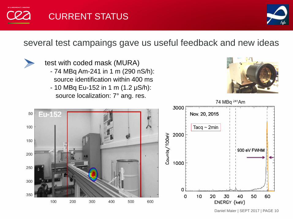
several test campaings gave us useful feedback and new ideas
Tacq = 0.4 s
test with coded mask (MURA) - 74 MBq Am-241 in 1 m (290 nS/h):
source identification within 400 ms
- 10 MBq Eu-152 in 1 m (1.2 μS/h):
source localization: 7° ang. res.
Eu-152 Am-241
CURRENT STATUS
Daniel Maier | SEPT 2017 | PAGE 10
several test campaings gave us useful feedback and new ideas
test with coded mask (MURA) - 74 MBq Am-241 in 1 m (290 nS/h):
source identification within 400 ms
- 10 MBq Eu-152 in 1 m (1.2 μS/h):
source localization: 7° ang. res.
Eu-152
CURRENT STATUS
Daniel Maier | SEPT 2017 | PAGE 11
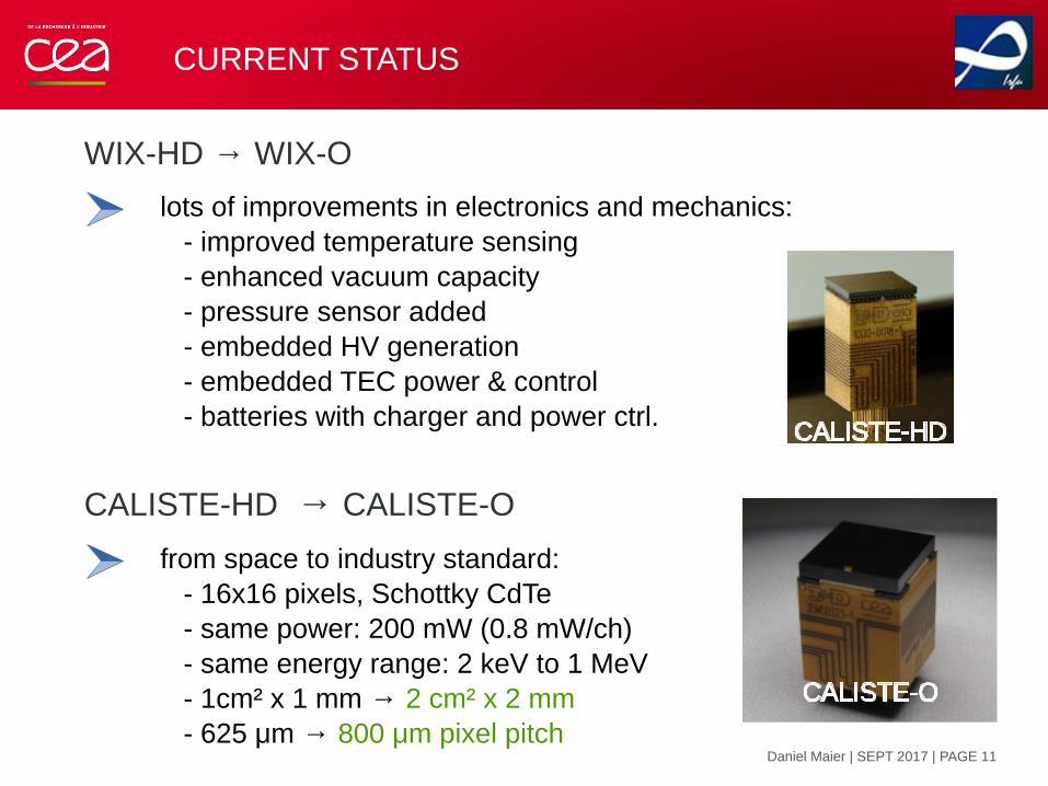
WIX-HD → WIX-O
lots of improvements in electronics and mechanics:
- improved temperature sensing
- enhanced vacuum capacity
- pressure sensor added
- embedded HV generation
- embedded TEC power & control
- batteries with charger and power ctrl.
from space to industry standard:
- 16x16 pixels, Schottky CdTe
- same power: 200 mW (0.8 mW/ch)
- same energy range: 2 keV to 1 MeV
- 1cm² x 1 mm → 2 cm² x 2 mm
- 625 μm → 800 μm pixel pitch
CALISTE-HD → CALISTE-O
CALISTE-HD
CALISTE-O

CURRENT STATUS
Daniel Maier | SEPT 2017 | PAGE 12
CALISTE-O
first tests show that all
pixel are working
spectral resolution: - best pixel: 927 eV FWHM @ 60 keV
- all pixel: 1.3 keV FWHM @ 60 keV
5 10 15 20 25 30 35 40 45 50 55 60 650
counts [ ]
5
10
15
20
25
30
35
40
20170626 122229, CALISTE-O, Am-241, 500V, tp2, LT15, singles
0
energy [keV]
counts [103]
0 2 4 6 8 10 12 14
0
2
4
6
8
10
12
14
x
y
20170626 122229, Am-241, 500V, tp2, LT15, all
2000 4000 6000 80000

CURRENT STATUS
Daniel Maier | SEPT 2017 | PAGE 13
CALISTE-O aims to detect gamma rays
Cs-137 source spectral resolution: - all pixel: 6.7 keV FWHM @ 662 keV
480
188
36.6
32.1
8.8
20170630_144111 Cs-137 only singles
100 200 300 400 500 600E [keV]
10
1000
100
1000
0
cnts []spectral features: - Cu fluorescence (8.8 keV)
- Ba Ka and Kb lines (32.1 & 36.6 keV)
- Ba* after Cs decay (662 keV)
- Compton scattering in the detector
(E < 480 keV)
- Compton scattering outside
(E > 188 keV)
- multiple (>2x) Compton sc.
det
662 keV
det
662 keV
det
662 keV
662

NEXT STEPS
Daniel Maier | SEPT 2017 | PAGE 14
we are not at the end...
test Compton imaging
autonomous control
autonomous analysis
point and interval estimations in x-, y-, and z-directions
combining mask and Compton
HV cycling to prevent CdTe instability
pixel individual trigger thresholds
optimal peaking time
energy calibration
source identification
flux / dose estimation

APPLICATION: medical physics
SATBOT:
radiotherapy + nano particles
Daniel Maier | SEPT 2017 | PAGE 15
biology
accumulation of NP
degradation of NP
5 Rs:
physics
enhanced absorption
because of high Z
generation of
generation of
fluorescence radiation
enhanced attenuation
-> dose enhancement
Auger e-
photo e-
Compton e-
chemistry
oxidative stress by
reactive oxigen species
(ROS):
H2O2
e- + H20 OH -
O2-
surface effec:
catalysator
coating
chemical enhancement
multidisciplinary field
Au
θX-ray tube
detector
repair,
redistribution
reoxygeneration
repopulation
radiosensitivity

BASIC PHYSICS
XRF detection
self absorptoin in humain tissue
Daniel Maier | SEPT 2017 | PAGE 16
depth
in s
oft tis
sue [m
m]
atomic number Z []
1
10
100
0 10 20 30 40 50 60 70 80 90
0
10
20
30
40
50
60
70
80
90
100
Kα1
absorp
tion
[%
]
100% 90%
80%
70%
60%
50%
40%
30%
20%
10%

BASIC PHYSICS
interaction photons ↔ humain
Daniel Maier | SEPT 2017 | PAGE 17
10-5
10-4
10-3
10-2
10-1
100
101
102
103
104
1 10 100 1000 10000
abs. coeff. μ
[1/c
m]
energy [keV]
ICRU4 coherent scattering
ICRU4 incoherent scattering
ICRU4 photo electric absorption.
ICRU4 pair creation (nucleus)
ICRU4 pair creation (atom)
bones
breast
blood
fat
ICRU 4 components

BASIC PHYSICS
XRF dosimetry
goal:- determine the concentration of the NP
- determine the dose at the
tumor level
Daniel Maier | SEPT 2017 | PAGE 18
~6
9 keV
t 1
d1
d2
t 2
human
tissue with
att. coef. μ1
tumor
+NP
human
tissue with
att. coef. μ2
detector
X-ray tube
F0
FILTER
F1 F2 F2 F3
F4
F5
F5
~7
8 keV
approach:
- prior knowledge of the tube flux
- determine the transmittivity t1 and t2
- tumor flux = tube flux * t1 →dose
- NP concentration ~ meas. flux / tumor flux
BASIC PHYSICS
Daniel Maier | SEPT 2017 | PAGE 19
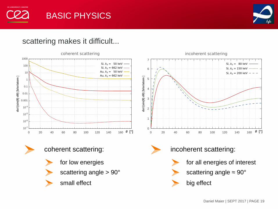
scattering makes it difficult...
coherent scattering:
for low energies
scattering angle > 90°
0
1
2
3
4
5
6
7
0 20 40 60 80 100 120 140 160
dσ
/(s
in(θ
) dθ)
[b
/sr/
ato
m ]
θ [°]
incoherent scattering
Si, k0 = 200 keV
Si, k0 = 150 keV
Si, k0 = 80 keV
10-7
10-6
10-5
10-4
0.001
0.01
0.1
1
10
100
1000
θ [°]
dσ
/(s
in(θ
) dθ)
[b
/sr/
ato
m ]
coherent scattering
Si, k0 = 50 keV
Si, k0 = 662 keV
Au, k0 = 50 keV
Au, k0 = 662 keV
0 20 40 60 80 100 120 140 160
small effect
incoherent scattering:
for all energies of interest
scattering angle ≈ 90°
big effect
SATBOT results
Daniel Maier | SEPT 2017 | PAGE 20
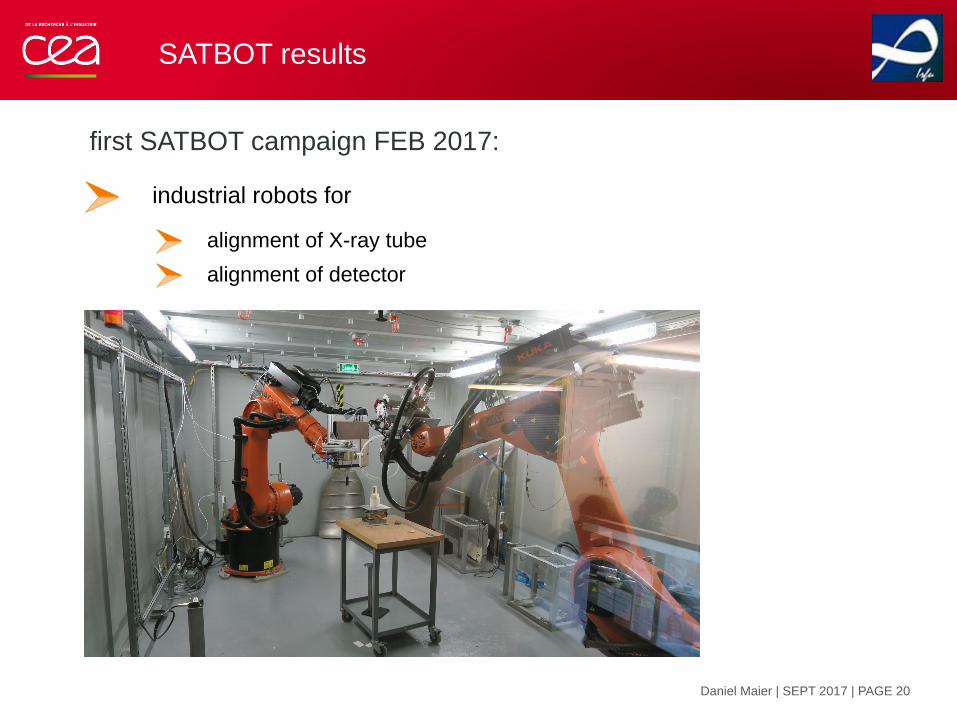
first SATBOT campaign FEB 2017:
industrial robots for
alignment of X-ray tube
alignment of detector

SATBOT results
Daniel Maier | SEPT 2017 | PAGE 20
first SATBOT campaign FEB 2017:
industrial robots for
alignment of X-ray tube
alignment of detector

SATBOT results
Daniel Maier | SEPT 2017 | PAGE 20
first SATBOT campaign FEB 2017:
industrial robots for
alignment of X-ray tube
alignment of detector
result
Au identification
independent of NP size
sensitivity: 408 ug Au Au / Kα
Au / Kβ
Nano en solution:
• 31 nm
• 45 nM
• 50 µL
22/2/2017
W / Kα
/ KβW

SATBOT results
Daniel Maier | SEPT 2017 | PAGE 21
second SATBOT campaign APRIL 2017:
filter for X-ray tube
shape the tube spectrum
enhance the high energetic part
result
Au identification for different mAu
lin. relation between signal & mAu
sensitivity: 380 ug Au
50 55 60 65 70 75 80
40000
60000
80000
100000
ENERGY (keV)
Counts, normal i zed
blanc
0,56 mg Au
1,12 mg Au
2,25 mg Au
problem:
detect a peak on top of a peak!

SATBOT results
Daniel Maier | SEPT 2017 | PAGE 22
third SATBOT campaign AUG 2017:
filter for X-ray tube
advaced filter
result
XRF peak in valley
clear Ka and Kb
detection
sensitivity:
Ka: 50 ug Au
Kb: 300 ug Au
Au Kα2 + Kα1
fit: SKα = 0.0949 cnt/(s cm2 μg) · m
Au Kβ3 + Kβ1
fit: SKβ = 0.0133 cnt/(s cm2 μg) · m
Au mass m [μg]
0 200 400 600 800 1000 1200 1400 1600 1800 2000 2200 2400
Au s
igna
l S
[c
nt/s]
0
50
100
150
200
250
2310 μg Au
1150 μg Au
577 μg Au
288 μg Au
144 μg Au
0 μg Au
20 40 60 80 100 56 60 64 68 72 76 80 84
flu
x [1
/(s k
eV
cm
2 )
]
E [keV] E [keV]0
0
20
40
60
80
100
60
50
70
80
90
detection limit
50 300

SATBOT new ideas: advanced X-ray filter
Daniel Maier | SEPT 2017 | PAGE 23
EXRF < K-edge
only E > K-edge causes XRF
background photons EXRF < E < K-edge → noise
X-ray filter without absorption edges
energy
transm
itta
nce
1
0
X-ray filter near an absorption edge
energy
transm
itta
nce
1
0
ideal X-ray filter
energy
transm
itta
nce
1
0
thin filter
thick filter
K-edge
unnecessary photons E < EXRF → unnecessary dose

SATBOT new ideas: advanced X-ray filter
Daniel Maier | SEPT 2017 | PAGE 23
EXRF < K-edge
only E > K-edge causes XRF
background photons EXRF < E < K-edge → noise
energytransmittance
1
0
usable
photons
for XRF
usable
photons
for XRF
n > 0
energy
transmittance
1
0Kedge, filter
Kedge, targetXRF
usable
photons
for XRF
n ≤ 0
energy
transmittance
1
0Kedge, filter
Kedge, targetXRF
usable
photons
for XRF
n << 0
XRF Kedge, targetKedge, filter
unnecessary photons E < EXRF → unnecessary dose
Zfilter = Ztarget + n
Combine filter with incoherent scattering
X-ray detector
(scintillator)
for transmitted radiation
ortho X-ray tube
(140 kV peak)
test sample
WIX X-ray camera
(CdTe) for fluorescence
and scattered radiation
X-ray
beam
scattered radiation loses energyTARGET
F
I
L
T
E
R
θX-ray beam
det.

SATBOT new ideas: advanced X-ray filter
Daniel Maier | SEPT 2017 | PAGE 24
0
5
10
15
20
25
30
35
40
45
50
55
60
65
70
75
80
85
90
0 5 10 15 20 25 30 35 40 45 50 55 60 65 70 75 80 85 90
Z []
Z []
n<< 0
n ≤ 0
n > 0
example: for Au: n≪0 for Z≤73
n<0 for 74 ≤ Z ≤79
n>0 for 80 ≤ Z ≤ 84

SATBOT new ideas: advanced X-ray filter
Daniel Maier | SEPT 2017 | PAGE 25
45
50
55
60
65
70
75
80
85
90
95
100
105
110
115
65 70 75 80 85 90
en
erg
y [ke
V]
atomic number Z []
20°30°40°
50°
60°
70°
80°
90°
100°
110°120°130°140°150°160°180°
Kedge
Kα1
Compton sc. Kedge color
θ
n=
1 n=
2
n=
-1
n=
3 n=
4 n=
5
n=
0
n=
-2
n=
-3
n=
-4
n=
-5
Which filter and which observation angle should we choose?

SATBOT new ideas: advanced X-ray filter
Daniel Maier | SEPT 2017 | PAGE 26
How thick should the filter be?
0
0.1
0.2
0.3
0.4
0.5
0.6
0.7
0.8
0.9
1
10 100 1000 10 000
cum
ula
tive p
hoto
ele
ctr
ic d
istr
ibution []
10-5
10-4
10-3
10-2
10-1
1.0
0 1000 2000 3000 4000 5000 6000 7000 8000 9000 10 000
rela
tive
photo
ele
ctr
ic c
ross s
ection []
E [keV] E [keV]
50050 5000
signal analysis:
flux
after
filter
flux
before
filter
SATBOT new ideas: advanced X-ray filter
Daniel Maier | SEPT 2017 | PAGE 27
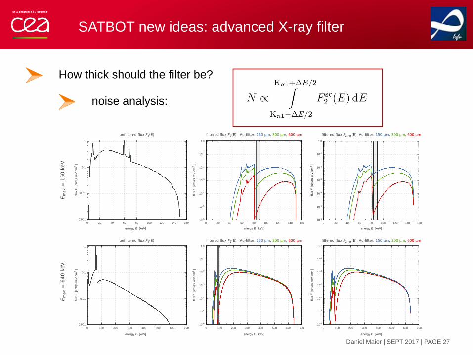
How thick should the filter be?
noise analysis:
0.001
0.01
0.1
1
0 20 40 60 80 100 120 140 160
flu
x F
[c
nt/(s
ke
V c
m2 ]
energy E [keV]
10-6
10-5
10-4
10-3
10-2
10-1
1.0
energy E [keV]
flu
x F
[c
nt/(s
ke
V c
m2 ]
0 20 40 60 80 100 120 140 160
flu
x F
[c
nt/(s
ke
V c
m2 ]
0 20 40 60 80 100 120 140 160
10-6
10-5
10-4
10-3
10-2
10-1
1.0
energy E [keV]
Em
ax =
15
0 k
eV
filtered flux F2(E), Au-filter: 150 µm, 300 µm, 600 µm filtered flux F2 res(E), Au-filter: 150 µm, 300 µm, 600 µmunfiltered flux F1(E)
0 100 200 300 400 500 600 700
0.001
0.01
0.1
1
flu
x F
[c
nt/(s
ke
V c
m2 ]
energy E [keV]
0 100 200 300 400 500 600 700
flu
x F
[c
nt/(s
ke
V c
m2 ]
energy E [keV]
10-6
10-5
10-4
10-3
10-2
10-1
1.0
energy E [keV]
flu
x F
[c
nt/(s
ke
V c
m2 ]
10-6
10-5
10-4
10-3
10-2
10-1
1.0
0 100 200 300 400 500 600 700
Em
ax =
64
0 k
eV
filtered flux F2(E), Au-filter: 150 µm, 300 µm, 600 µm filtered flux F2 res(E), Au-filter: 150 µm, 300 µm, 600 µmunfiltered flux F1(E)

SATBOT new ideas: advanced X-ray filter
Daniel Maier | SEPT 2017 | PAGE 28
How thick should the filter be?
maximize signal-to-noise ratio
0.00000
0.00025
0.00050
0.00100
0.00200
0.00400
0.01000
0.02000
0.04000
0.08000 0.1
1
10
100
0 0.2 0.4 0.6 0.8 1
SN
R []
filter thk [mm]
Gold (Z = 80; n = 0; θ = 130°)add a constant
background flux

SATBOT new ideas: advanced X-ray filter
Daniel Maier | SEPT 2017 | PAGE 29
How thick should the filter be?
a filter can make it worse
a higher voltage of the X-ray tube makes the SNR always better ;-)
the optimal filter thickness is independent of the chosen voltage

SATBOT conclusions
Daniel Maier | SEPT 2017 | PAGE 30
SATBOT is a very dynamic project
the work is very interdisciplinary
next steps:
new filter: sensitivity < 20 ug
XRF tomography

SATBOT conclusions
Daniel Maier | SEPT 2017 | PAGE 31
the SATBOT team is very nice