call admission control and dynamic pricing in a … admission control and dynamic pricing in a...
TRANSCRIPT

Call Admission Control and Dynamic Pricing in a GSM/GPRS Cellular Network
by
Alan Olivré
A dissertation submitted to the University of Dublin,
in partial fulfillment of the requirements for the degree of
Master of Science in Computer Science
Department of Computer Science, University of Dublin, Trinity College
September, 2004

Declaration
I declare that the work described in this dissertation is, except where otherwise stated, entirely my
own work and has not been submitted as an exercise for a degree at this or any other university.
Signature of Author…………………………………………….……………………………………
Alan Olivré
13, September, 2004

Permission to lend and/or copy
I agree that Trinity College Library may lend or copy this dissertation upon request.
Signature of Author……………………………………………………….…………………………
Alan Olivré
13, September, 2004

Acknowledgements
I would like to thank Mélanie Bouroche for all the time she spent answering my numerous
questions and for the excellent work she did last year, which was of great help.
I would also like to thank my supervisor, Meriel Huggard, for her enthusiasm and her time
throughout the duration of this project.
Thanks to the whole NDS class for their friendship and help during this long and demanding year,
and especially to Shane, who made me see some of the famous places of this beautiful country.
Finally, special thanks to my family, to Cédric and to Sandrine, for all that they have done and
without whom I would have given up a long time ago.

Abstract
In the past decade, the wireless communications market has experienced tremendous growth, and
this growth is likely to continue in the near future. In addition to an increase in the number of
users, ever more demanding applications will appear, resulting in ever greater resource
requirements. The limited radio frequency spectrum available can no longer support this
increasing demand, and the required quality of service will no longer be attainable if an efficient
solution is not found.
The easiest approach to solve this problem is to increase the capacity of the network, but this is
uneconomic and not really practical. Indeed, at their current size, the networks are already under
utilized most of the time, even if they can not accept every incoming call during congested peak
periods. Increasing their capacity still further may solve the congestion problem for a while, but
at the cost of an even higher global under utilization of resources. Other solutions have emerged
to alleviate this problem, but none of them is really effective when the degree of congestion
becomes too high.
An alternative solution is to keep the current network capacity and to make the users’ demand fit
this limited capacity. This is the basic principle which leads to dynamic pricing: the price of
making a call depends on the network load, it can be very high when congestion occurs or very
low to encourage users to make calls during off-peak periods. As a result, the congestion is
decreased while the overall utilization of the communications channels is improved. Dynamic
pricing has already been applied successfully in several domains, but has only recently been
considered for use in cellular networks. This project aims to look at how the different solutions
mentioned above perform to solve the problem of congestion in the case of both GSM and
GSM/GPRS networks, and in particular, at whether or not a combination of dynamic pricing and
more traditional approaches can give better results. For this purpose, a detailed traffic model for
both GSM and GPRS networks is given and implemented in an event-driven simulator. The effect
of several dynamic pricing and admission control combinations is then analysed, and the
importance of some incoming traffic parameters is highlighted.

i
Content Introduction ..............................................................................................................................1
1.1 Context.......................................................................................................................1
1.2 Project Goal ...............................................................................................................2
1.3 Contribution to Knowledge.........................................................................................3
1.4 Dissertation Outline....................................................................................................4
State of the Art in Dynamic Pricing..........................................................................................5
2.1 Dynamic Pricing in Mobile Networks .........................................................................5
2.1.1 A Self-regulated Dynamic Pricing Algorithm for GSM/GPRS Networks ............5
2.1.2 Integration of Pricing with Call Admission Control for Wireless Networks.......11
2.1.3 Dynamic Pricing for Connection-oriented Services in Wireless Networks.........16
2.1.4 Models for 3G/4G Network Pricing..................................................................18
2.2 Dynamic Pricing in Other Industries .........................................................................19
2.2.1 Internet/ATM...................................................................................................19
2.2.2 Fixed Telephony ..............................................................................................22
2.2.3 Electricity ........................................................................................................22
2.2.4 E-Commerce....................................................................................................22
2.2.5 Market .............................................................................................................23
2.3 Conclusions..............................................................................................................23
Channel Allocation and Call Admission Control ...................................................................24
3.1 Channel Allocation...................................................................................................24
3.1.1 Fixed Channel Allocation.................................................................................25
3.1.2 Dynamic Channel Allocation............................................................................26
3.1.3 Hybrid Channel Allocation...............................................................................26
3.2 Call Admission Control ............................................................................................27
3.2.1 Simple CAC Schemes ......................................................................................27
3.2.2 Advanced CAC Schemes .................................................................................30
3.3 Conclusion ...............................................................................................................34
GSM/GPRS Network Modelling.............................................................................................35
4.1 GSM and GPRS Technologies ..................................................................................35

ii
4.1.1 GSM................................................................................................................35
4.1.2 GPRS...............................................................................................................36
4.1.3 Resources allocations between GSM and GPRS ...............................................38
4.2 Cellular Network Modelling .....................................................................................38
4.2.1 Basic Approach................................................................................................38
4.2.2 Classic Approach .............................................................................................39
4.2.3 Refined Approaches .........................................................................................39
4.3 Traffic Modelling .....................................................................................................40
4.3.1 GSM................................................................................................................41
4.3.2 GPRS...............................................................................................................41
4.4 Call duration and cell dwell times .............................................................................47
4.5 Conclusion ...............................................................................................................48
Simulator .................................................................................................................................49
5.1 Design of the Simulator ............................................................................................49
5.1.1 Type of Simulator ............................................................................................49
5.1.2 Level of Abstraction.........................................................................................49
5.1.3 Functioning of the Simulator ............................................................................50
5.2 GPRS Traffic............................................................................................................52
5.2.1 Introduction .....................................................................................................52
5.2.2 Representation of a GPRS Call.........................................................................53
5.3 Features of the Simulator ..........................................................................................55
5.4 Simulator Validation ................................................................................................55
5.5 Conclusion ...............................................................................................................56
Experiments and Results.........................................................................................................57
6.1 Steady State..............................................................................................................58
6.1.1 Experiment ......................................................................................................58
6.1.2 Results .............................................................................................................58
6.2 Guard Channels ........................................................................................................59
6.2.1 Experiment ......................................................................................................59
6.2.2 Results .............................................................................................................59
6.2.3 Conclusion.......................................................................................................61
6.3 Queuing Schemes .....................................................................................................61
6.3.1 Experiment ......................................................................................................61

iii
6.3.2 Results .............................................................................................................62
6.3.3 Conclusion.......................................................................................................66
6.4 Channel Borrowing ..................................................................................................66
6.4.1 Experiment ......................................................................................................66
6.4.2 Results .............................................................................................................66
6.4.3 Conclusion.......................................................................................................68
6.5 Dynamic and Hybrid Channel Assignment (DCA & HCA) .......................................69
6.5.1 Experiment ......................................................................................................69
6.5.2 Results .............................................................................................................69
6.5.3 Conclusion.......................................................................................................71
6.6 Conclusion About the Experiments Carried Out Considering GSM Only ..................71
6.7 Inclusion of GPRS Traffic ........................................................................................73
6.7.1 Influence of the Pricing Scheme .......................................................................74
6.7.2 Influence of Incoming Traffic Division ............................................................77
6.7.3 Influence of the Number of GPRS Channels.....................................................80
6.7.4 Influence of the Maximum Number of GPRS Channels per Call.......................83
6.7.5 Conclusion About the Experiments Carried Out With GPRS ............................85
6.8 Conclusion ...............................................................................................................85
Conclusions..............................................................................................................................87
7.1 Achievements...........................................................................................................87
7.2 Obstacles Overcome .................................................................................................90
7.3 Future Work .............................................................................................................90
Bibliography............................................................................................................................92

iv
List of figures
Figure 1 : Basic Algorithm ..........................................................................................................6
Figure 2 : Complete Algorithm..................................................................................................11
Figure 3 : System structure for Hou et al.’s algorithm ................................................................13
Figure 4 : Utility function with hard QoS requirements..............................................................14
Figure 5 : Utility function with soft QoS requirements...............................................................15
Figure 6 : Birth-death Markov chain..........................................................................................17
Figure 7 : Channel allocation for N=3 and N=7 .........................................................................25
Figure 8 : Channel locking ........................................................................................................26
Figure 9 : Shadow cluster ..........................................................................................................32
Figure 10 : Notion of threshold distance ....................................................................................33
Figure 11 : Adaptive channel reservation...................................................................................34
Figure 12 : Throughputs for GPRS in kbits/s .............................................................................37
Figure 13 : Refined approach model 1 .......................................................................................40
Figure 14 : Refined approach model 2 .......................................................................................40
Figure 15 : Incoming traffic as a function of the time of day ......................................................41
Figure 16 : Traffic repartition for dial-in users ...........................................................................42
Figure 17 : Model of Choi and Limb for Web traffic..................................................................44
Figure 18 : Simplified class diagram..........................................................................................50
Figure 19 : Event hierarchy .......................................................................................................51
Figure 20 : Representation of a GPRS call .................................................................................53
Figure 21 : State of channels before and after GPRS call ...........................................................54
Figure 22 : Utility as a function of time in the Steady State........................................................58
Figure 23 : Revenue as a function of N......................................................................................60
Figure 24 : Utility as a function of N .........................................................................................60
Figure 25 : N as a function of time ............................................................................................61
Figure 26 : Percentages of calls queued as a function of time.....................................................64
Figure 27 : Percentages of calls being queued as a function of time 2.........................................64
Figure 28 : Number of attempts before treatment as a function of time.......................................65
Figure 29 : Number of attempts before treatment as a function of time 2....................................65
Figure 30 : Number of channels borrowed and lent as a function of time....................................67
Figure 31 : Number of channels borrowed and locked as a function of time ...............................68
Figure 32 : Number of channels in pool as a function of time.....................................................70

v
Figure 33 : % of calls using channels in pool as a function of time.............................................71
Figure 34 : Revenue as a function of time without pricing .........................................................75
Figure 35 : Variation of revenue over a day with pricing............................................................76
Figure 36 : Average number of channels allocated as a function of time.....................................77
Figure 37 : Revenue as a function of % GPRS without pricing...................................................78
Figure 38 : Total revenue as a function of % GPRS with pricing................................................79
Figure 39 : Utility as a function of % GPRS calls ......................................................................79
Figure 40 : Total revenue with number of GPRS channels without pricing.................................81
Figure 41 : Total utility with number of GPRS channels without pricing....................................82
Figure 42 : Total revenue as a function of the maximum number of channels per call, without
pricing ..............................................................................................................................83
Figure 43 : Total revenue as a function of the maximum number of channels per call, with pricing
.........................................................................................................................................84

vi
List of tables
Table 1 : Model used for Web Traffic........................................................................................45
Table 2 : Results for the experiments carried out with GSM only...............................................72

1
Chapter 1
Introduction
1.1 Context In the past decade, the wireless communications market has experienced tremendous growth, and
this growth is likely to continue in the near future. In addition to an increase in the number of
users, ever more demanding applications will appear, resulting in ever greater resource
requirements. The problem for wireless networks is that the available radio frequency spectrum is
limited, and can no longer support this increasing demand. The original approach used to solve
this problem was to increase the capacity of the network using cell splitting and frequency reuse
[78], or overlapping cell layers [79]. But this can not continue indefinitely. Nowadays, the
number of cells in large cities has almost reached its maximum, and reducing the size of the cells
still further would add more technical overheads than capacity benefits. Moreover, during off-
peak periods, it would increase the amount of unused resources, which is uneconomic from the
operators’ points of view and is, thus, to be avoided.
Since it is no longer possible to make the network capacity fit the demand during peak periods,
alternative solutions have to be found to achieve a better utilization of this limited capacity. One
of these is to manage the incoming calls more efficiently, in order to guarantee a satisfactory level
of quality of service (QoS). This can be achieved using one of the call admission control (CAC)
schemes developed over the past few years [37-45]. The role of a CAC scheme is to decide
whether a call should be allowed to enter the system or not, by taking into account different QoS
parameters. In mobile networks this decision is made more difficult by the existence of two types
of call: new calls which wish to connect to the network and handoff calls that started in one cell
and are willing to continue in another. Since it is more annoying from a user’s point of view to
lose an ongoing call than to see a connection attempt refused, most of the schemes are designed to
favour handoff calls whilst keeping the tradeoff between handoff and new call blocking at its
optimal value. A second solution is to use more efficient algorithms to manage the number of
available channels, only allocating them to the cells which require them, instead of giving all cells
the same number of channels regardless of the number of users they have to cope with. This has
given rise to dynamic and hybrid channel allocation schemes [28].

2
Even if the previously mentioned techniques can improve the users’ level of satisfaction when the
network is not congested, it has been proven that their performance starts declining as soon as the
number of users exceeds a certain limit. This means that there is a need to avoid congestion by
making demand fit the available capacity, since the opposite is impossible in some cases. Because
a user tends to act selfishly, using the maximum available resources even if it decreases other
users’ level of satisfaction, the only possible solution is to use price as a mechanism to give
incentives to make a call or not. This leads to real-time or dynamic pricing: the price per unit of
time will change in real-time according to network load. A high price during periods of
congestion will make some users postpone their calls or shorten them. Similarly, they can try to
move to another cell to obtain a cheaper price. On the contrary, a very low price could encourage
the users to make their calls at times they did not want to originally. The overall result will be a
better distribution of the calls during the day, a reduction of peak time congestion and a better
utilization of the resources during off-peak times. This is an important step forward from the
pricing strategy used by most mobile telephony operators, who charge different prices during
periods that they think will be over or under loaded, but who do not take the actual network load
into consideration.
Dynamic pricing, albeit having being used for a long time for regulating the traffic on packet-
based networks, such as the Internet, is only emerging now as a potential solution to congestion
problems in cellular networks. Economic and user behaviour studies, as well as technical ones,
have to be made prior to its use to determine the best pricing functions to use in order to achieve
the best possible results. This type of pricing could then be applied to cellular networks in
addition to existing techniques, where its effects as a traffic regulator are much needed.
1.2 Project Goal Although CAC schemes and dynamic pricing were designed for the same purpose, little work has
been carried out on their combined effects as a resource manager. The principal study, [8], is
more focused on dynamic pricing and the call admission control scheme it uses is relatively
simple. Hence, it does not explore all the possible benefits a well designed CAC scheme has to
offer. Therefore, it would be worthwhile and beneficial to explore how different CAC schemes
manage to improve the network utilization, and how well they can be combined with dynamic
pricing. This could permit direct comparison and allow for the determination of the best scheme,

3
as well as presenting how dynamic pricing can provide even greater results. This is one goal of
this project.
With the current trend towards an ever growing use of mobile networks for purposes other than
simple voice calls, there is a need to understand how dynamic pricing would behave in the case of
packet-based cellular networks, since these may be used in the future. This is a second goal of
this project: to explore how incoming traffic properties, mixing both GSM and GPRS calls, could
impact on network performance, and to seek the best values for key parameters.
Finally, a third goal of this project is to continue the work begun in [50], where an accurate model
of a GSM/GPRS cellular network was established by surveying the associated literature. This
model needs to be deepened to incorporate new applications using GPRS technology, such as file
or e-mail transfer. By integrating such improvements, the simulator built for [50] will be made
more powerful in the sense that it will have more features and that it will allow the user to have
access to more experimental settings.
1.3 Contribution to Knowledge For this work, the main studies on GSM and GPRS network modelling have been analyzed and
compared in order to determine which is most suited as a model for a cellular network which
includes e-mail and file transfer. The chosen model may now be used for further studies where an
accurate model is required, or used as a basis on which other technologies or applications models
can be built.
Different combinations of call admission control schemes and dynamic pricing have been studied
through simulation, and their comparative benefits analyzed using two important metrics: the
total revenue and the total utility generated over a day.
Finally, the importance of some of the incoming traffic parameters has been outlined and their
optimal values considered from the perspective of performance.
Together these should lead to a better understanding of how dynamic pricing behaves and how it
could be used in current cellular mobile networks.

4
1.4 Dissertation Outline In the following chapter, recent research studies on dynamic pricing are reviewed. This includes
detailed descriptions of the small number of dynamic pricing algorithms that have been proposed
for cellular networks, along with a recapitulation of the results obtained when these are applied to
other technologies. In chapter 3, existing call admission control and channel assignment schemes
are presented. Chapter 4 is a presentation of the existing work from which the network model
used by the simulator was derived. The simulator built for this work is then described in chapter
5, together with the GPRS traffic model adopted. Finally, the experiments carried out using the
simulator and the results obtained are presented in chapter 6, before the conclusions drawn are
discussed in chapter 7.

5
Chapter 2
State of the Art in Dynamic Pricing
In this chapter, we review the different dynamic pricing schemes proposed in the literature for
different technologies with a particular focus on mobile networks. Dynamic pricing in cellular
networks has only recently become a research domain, and not many comprehensive studies have
been completed. Indeed, only three significantly different approaches have been identified in the
literature. The first of these has been proposed by Fitkov-Norris and Khanifar, the second by Hou,
Yang and Papavassiliou and the last by Viterbo and Chiasserini. In marked contrast, dynamic
pricing for packet based networks such as the Internet has been a centre of research interest for
quite some time, and numerous studies have been undertaken [14-17]. Some of the most relevant
ones to this work will be described herein. Finally, conclusions drawn about dynamic pricing in
other contexts like electricity, fixed telephony or E-Commerce will be detailed and similarities
with mobile networks will be outlined.
2.1 Dynamic Pricing in Mobile Networks
2.1.1 A Self-regulated Dynamic Pricing Algorithm for GSM/GPRS Networks
2.1.1.1 Presentation
In [1-4] Fitkov-Norris and Khanifar introduce one of the first dynamic pricing algorithms for
mobile networks. The basic algorithm appears rather simple, but is based on a number of well
accepted principles. Among these is the fact that as price increases users tend to both shorten the
duration of their calls and reduce the number of calls made. Therefore, pricing strategy is a very
powerful tool for maintaining the network load (which is a function of the average call holding
time and the call inter-arrival times) at a predefined level where the degree of user satisfaction is
considered acceptable. However, the nature of mobile networks makes it necessary for even the
simplest algorithm to take into account parameters such as the price elasticity on demand or the
impact of pricing on mobility, resulting in complex equations from even a simple starting point.

6
The algorithm itself is self-regulated: it uses a number of predefined parameters and regularly
checks the conformity of the actual load of the system to these parameters. If it is decided that the
network requires a price adjustment, a tariff increment ∆P is calculated and the price is updated.
∆P can be positive or negative. If it is positive, then the load on the system is too high, and the
users’ degree of satisfaction may suffer as a consequence. The newly introduced higher price will
act as an incentive for new users to wait for a while before making their calls, thus reducing the
traffic load. On the contrary, if ∆P is negative, it means that the resource is not optimally used,
and that a part of the network is available. A lower price should encourage the consumers to make
their calls. The speed at which this price update is made determines the level of self-regulation of
the system.
A representation of the basic algorithm can be seen in figure 1 below. The complete algorithm
including both GSM and GPRS traffic is given in figure 2. GSM and GPRS traffic are different
(see chapter 4). Hence, it can not seem obvious how the same pricing algorithm may be applied to
both of them. Fitkov-Norris and Khanifar argue that this is possible because GSM and GPRS
share the same pool of resources. Whereas GSM (voice) calls can only use one channel at a time,
the advantage of GPRS is that the bandwidth can be greatly increased by the allocation of several
timeslots to one call. The pricing strategy should consequently be based on the bandwidth used. If
the nominal price for the usage of one channel for a particular duration is known, it is possible to
calculate the corresponding price for calls with multiple channels.
Figure 1 : Basic Algorithm

7
2.1.1.2 Implementation
According to the authors, the most suitable position for implementation of the algorithm will be
in the Base Station Controller (BSC). They provide three major justifications for their choice. The
first is that the BSC already collects the information used by the algorithm (revenue, number of
calls blocked, etc.) without using it. The second is that the calculation of the algorithm in real
time requires sufficient processing power, which can be found in the BSC. Finally, the
positioning of the algorithm in the BSC would minimize the increase in the control traffic
overhead in the network.
Once the price calculation is finished, the result can be broadcast to the mobile stations in the
target cell using the Broadcast Control Channel, since this channel is only listened to by the
Mobile Stations in that particular cell and has a free slot on the downlink.
2.1.1.3 Algorithm Details
Up to now, only a general description of the algorithm behaviour has been given along with a
possible implementation strategy. In this subsection, the user behaviour model is detailed and the
pricing scheme presented.
2.1.1.3.1 User behaviour model
Call Generation Rate
The user demand is modelled as a combination of a deterministic function D(t), a function of the
time of day which can be predicted fairly accurately, and a random demand S(t) caused, for
example, by emergencies.
D(t) is modelled using a Markov-modulated traffic model [5]. The call inter-arrival times are
determined by the generation rate, which is a function of the time of the day. The probability of K
arrivals in interval of length t is given by:

8
tK
K eKttP λλλ −=!)()(
(1)
Effect of price on demand
The effect of price on demand is modelled using an exponential function:
XQPX eAQ β−= . (2)
Where:
- XQ is the quantity demanded of good X,
- XQP is the price of good X,
- A is the demand shift constant,
- β is the demand elasticity coefficient.
This equation is a simplification of the actual function used. In reality, two additional parameters
are taken into account.
• The demand shift constant A captures the change in demand due to the effect of the time
of day. It uses historical data and will, therefore, change in time. Since pricing bias is
already present in the historic data due to the pricing schemes in place, the model is
corrected by taking the difference between the peak or off-peak price in the real system
and the dynamic price in the modelled system.
• If the dynamic price drops below the historic off-peak price, a fixed line substitution
effect is taken into account using an exponential function.
The modified version of equation 2 is, therefore,
ββ −−− −+= )().( )(dynamicbias
PPX PPEetAQ dynamicbias
(3)

9
where E is the off-peak shift constant.
Effect of price on mobility
Regretfully, this information is not available for telecommunications, because no study about it
has been carried out. Hence an alternative approach had to be used. The gravity model has been
borrowed from economics for use in this algorithm. Wilson originally employed it to determine
the most probable distribution of the number of trips between two regions depending on the
attractiveness of the destinations [6]. The translation of this model to the mobile network scenario
is very straightforward, so the adaptation of the model was an easy task.
The resulting model is given by the following formula:
=
ijjiij d
OOK 1..ψ
where:
- K is a constant
- ijψ is the total number of calls between cells i and j.
- ijd is the price of the calls.
- iO is the total number of users in cell i.
The drawback of this formula is that it is not linear: if the number of users doubles in cell i and in
cell j, the number of expected calls will quadruple; therefore corrective constants iA and jB
need to be introduced. The gravity model is thus modified to:
)(.... ijjijiij dfOOBA=ψ
with:
∑=
j ijjji dfOB
A)(..
1
∑=
i ijiij dfOA
B)(..
1

10
where )( ijdf is the pricing function.
2.1.1.3.2 Pricing
In a dynamically priced network, the shape of the pricing function is the most important
parameter, as it influences the demand function and consequently the total revenue and utility of
the network.
In [4], two pricing functions, linear and non-linear, have been tested. In [2], a more complex
function is introduced. This is the solution of the following minimization problem:
+∫
max
0 min )).((Q
dqqPPMin subject to Mdqqp =+ 2)'(1
The solution is of the form: 22min )()( qhPKqP −−−−= λ
It is also possible to adapt the pricing strategy to the desired goals. Therefore, a pricing function
which aims at optimizing the revenue or the total utility can be designed. It should be noted that
there is a natural trade-off between these design strategies.
2.1.1.3.3 Results
This dynamic pricing strategy has been tested through simulation [1-2]. The results show that the
total revenue generated is significantly higher than that generated with existing pricing schemes
and that the rate of call blocking is much lower than with the current schemes (the overall
reduction is as high as 30%). It is thus shown that dynamic pricing is a very efficient tool for
regulating the network load and, moreover, has other significant advantages.

11
Figure 2 : Complete Algorithm
2.1.2 Integration of Pricing with Call Admission Control for Wireless Networks
2.1.2.1 Scheme Proposed
In [7-8], Hou, Yang and Papavassiliou present a new dynamic pricing scheme for cellular
networks. The main improvement, in comparison to the scheme described above, is that it
introduces the notion of call admission control. Whereas the previous scheme did not consider the
difference between new calls and handoff calls (calls started in a cell but which will be continued
in another cell because the user is moving), this one does. Numerous call admission control

12
strategies exist, as will be explained in the next chapter, most of them designed to manage the
natural trade-off between new calls and handoff calls in a cell: if the decision is made to give the
priority to handoff calls for example, it will consequently increase the probability that new calls
are blocked, and vice-versa.
Hou et al. argue that traditional CAC schemes are not sufficient, because they can not ensure a
good quality of service when the network is congested. When the number of ongoing calls
becomes too high then, no matter what CAC scheme is used, the probability that new calls or
incoming handoff calls are blocked becomes too high to give the users a good level of
satisfaction. In that context, the introduction of pricing as a new dimension to call admission
control is a way to maintain the resource utilization to an optimal level, whilst ensuring a
predefined quality of service (or utility). Their research focuses on optimizing the resource
utilization rather than the total revenue. However, the two are linked since the price is set at the
maximum price for which all the resources are used.
2.1.2.2 Definition of the Optimal Call Arrival Rate
In [7], it is proved analytically that, for a given network (with a predefined set of parameters such
as the number of channels per cell, and a chosen CAC scheme) and under further assumptions
about the shape of the utility function, there exists a call arrival rate which maximizes the total
utility. The total utility is the sum of the utility of the individual users, the latter being a
representation of the users’ welfare. In this case, it is a function of a weighted sum of the new call
blocking probability and the handoff call blocking probability. The coefficient associated with
handoff calls is more important, as it is more damaging for a user to lose an ongoing call than to
be unable to establish a new call. Therefore, the aim of the pricing scheme is to maintain the
arrival rate as close as possible to this optimal arrival rate.
2.1.2.3 Experimental Settings
2.1.2.3.1 System Structure
The system is composed of two independent blocks, the pricing block and the CAC block. A
Guard Channel CAC scheme is used; as will be explained in the next chapter, this gives priority
to handoff calls by blocking new calls if the number of available channels is less than the

13
designated number of guard channels and by blocking handoff calls only if all channels are
occupied.
The system is described in figure 3 below.
Figure 3 : System structure for Hou et al.’s algorithm
When a user attempts to establish a connection, the new call is first considered by the pricing
block, and the user given the current price. If the price is accepted, the call is forwarded to the
CAC block, where it can be either accepted or rejected, depending on the prevailing network
load. If the price is too high, the user can either leave or retry after a delay.
2.1.2.3.2 Pricing Strategy
The price charged to the user depends on the network load, as expected in a dynamically priced
network. However, contrary to the pricing scheme proposed by Fitkov-Norris and Khanifar, the
main concern is the user utility; the price can not become very low as a means to encourage the
user to make more calls when the network is under-utilized. Consequently, the pricing strategy is
as follows: when the incoming rate λ is less than the optimal rate λ*, a constant price 0p is
charged. When it becomes more than λ*, a dynamically calculated price p(t) is charged.
2.1.2.3.3 Demand Modelling
The demand function is that introduced in [9]:
2
0)1)((
)]([−−
= ptp
etpD for p(t) ≥ 0p

14
D[p(t)] represents the percentage of users who will accept the current price. Since D[ 0p ] = 1, it
means that 0p is accepted by everyone.
2.1.2.3.4 Pricing Function
The price p(t) to be charged at a particular time t is given by the following function, which is a
function of the new call arrival rate, the retry call arrival rate as represented in figure 3 above, and
the optimal call arrival rate.
+
= − )1,)()(
min()(*
1
ttDtp
rn
n
λλλ
2.1.2.3.5 Utility Function
The utility function needs to be a good representation of how the network load impacts on the
users’ welfare. It is obvious that it must be a decreasing function of the global blocking
probability, but a lot of different shapes are acceptable. Two main approaches can be used. The
first corresponds to a system with hard QoS requirements, whereas the second corresponds to a
system with softer ones.
A utility function of the first type can for example be:
)1.0(301 1 −−= PbeU for 0 ≤ Pb ≤ 0.01 and 0 otherwise
Figure 4 : Utility function with hard QoS requirements

15
A utility of the second type can be:
)0,1max( )1.0(.302
−−= PbeU
Figure 5 : Utility function with soft QoS requirements
The former is used in the original study [8].
2.1.2.4 Results
This model has also been evaluated through simulation. The call arrival rate is described by a
Poisson Process and the call holding time follows a negative exponential distribution. Contrary to
the experiments carried out by Fitkov-Norris and Khanifar, the call duration is independent from
the price.
Different user behaviours were considered, with regards to the percentage of users that retry after
being blocked at the pricing level and at the CAC level. The results were also compared with the
case where no pricing block was implemented.
It was shown that the proposed system, which integrates CAC and dynamic pricing, succeeds
where traditional CAC schemes fail, that it to say, in guaranteeing a predefined level of QoS even
during the peak periods. Moreover, both the total user utility and the operator revenue are
significantly increased.

16
2.1.3 Dynamic Pricing for Connection-oriented Services in Wireless Networks
2.1.3.1 Presentation
In [10, 11], yet another approach to dynamic pricing in connection-oriented mobile networks is
presented. The main goal of this research is to maximize the total revenue by finding an optimal
pricing function.
The call duration is modelled as a function of the service price, and the user demand as a
decreasing exponential function of both the call price per unit of time and the call blocking
probability, which is the Quality of Service metric they selected.
In addition, because customers like transparency, the price follows an imposed linear dynamic.
Standard Markovian techniques are used to represent the system evolution and to determine the
optimal pricing function.
2.1.3.2 System Model
2.1.3.2.1 Demand Modelling
A standard econometric model is used for the demand function:
)(),( QpeQpD βα +−=
where p is the price per unit of time and Q is the Quality of service. Here, the quality of service is
said to be the probability of call success, that is Q = 1 - Pb where Pb is the probability of a call
being blocked. The parameters α and β characterize the user population behaviour and must be
identified by adequate market research.
This model takes into account common user behaviour: the users’ demand function drops as the
price per time unit increases and the quality of service decreases.
If the system is supposed to have N communication channels, it may be represented by a birth-
death Markov chain where each state i = 0, … N represents the number of ongoing calls.

17
Figure 6 : Birth-death Markov chain
iλ is the call arrival rate when the system is in state i, and iµ is the average call termination rate
when the system is in state i. ),...,,( 110 −= Npppp is the price vector representing the cost per
time unit of a call started when the system is in state i. The objective is to determine the optimal
price vector which will maximize the total revenue while reducing the blocking probability.
Applying standard Markovian techniques to the Markov chain given above, the steady state
solution is given by the following probability vector ),...,,( 10 Nπππ where
1
01
10
−
==
−
= ∑ ∏N
k
k
j j
j
µλ
π and ∏=
−=i
j j
ji
1
10 .
µλ
ππ
The blocking probability can be deduced as being equal to Nπ . Knowing the price vector and the
probability vector given above, it is easy to calculate the total revenue generated while
maintaining the blocking probability at a satisfactory level. The optimization problem is now only
a very complex mathematical problem.
2.1.3.3 Results
The results have been obtained for different user populations (by varying the coefficients α and β)
and compared to a flat pricing strategy where a constant price for the network usage is fixed. It is
shown that when the traffic load is very low, the dynamic pricing strategy may lead to a slight
loss of revenue. However, as soon as the traffic load increases, the dynamic strategy behaves
much better and results in a huge increase of revenue (more than 25%). It is also noted that α and
β have little impact on the results.

18
2.1.3.4 Future work
The first part of the research study, as presented above, only considers connection-oriented
communications. A future objective of Viterbo and Chiasserini is to apply the same Markovian
techniques to packet-based networks. They want to consider third generation mobile
communications, where different classes of users can be introduced given their desired
information bit rate and actual bandwidth occupancy. They propose not to use the basic idea,
which would be to charge the user according to B (bandwidth used) and to the traffic load.
Instead, they intend to apply a different pricing strategy to each user class.
The same demand function as for the connection oriented systems is used for each user in each
class, and then multi-dimensional Markovian techniques are used to solve the problem.
2.1.4 Models for 3G/4G Network Pricing
Wallenius and Hamalainen presented models for 3G/4G service pricing including QoS guarantees
[12].
Two types of pricing for the different 3GPP (3rd Generation Partnership Project) [13] traffic
classes are introduced. For real-time connections, which are always given a whole traffic channel,
it is possible to charge based on the duration and on the number of bits transmitted. For non real-
time interactive and background classes, however, a pricing function of the reserved bandwidth is
considered more suitable.
Because linear pricing functions for QoS provision can result in huge disparities between
connections with high requirements (multimedia) and connections with low ones (voice), a
linearity factor is introduced.
The price is then as follows: lxB
ijb TeeAP ).( .−−=
Where:
- bP is the unit of price of the call
- ijA is the linear price factor for each traffic and subscriber class
19
- lT is the traffic load
- B is a linearity parameter
- x is one of the QoS attributes, which can be either bandwidth, end to end delay or bit
error rate
2.2 Dynamic Pricing in Other Industries
2.2.1 Internet/ATM
Contrary to the case of Mobile Networks, dynamic pricing as a means of congestion avoidance
has been investigated in detail for packet-based networks, such as the Internet or ATM.
There are two main methods to dynamically price the Internet. You can make the users pay
according to prices they bid for available bandwidth, or make them pay according to the
congestion they cause to other users. The first is called Smart-Market, the second Shadow-
pricing. The two approaches are linked, because the more bandwidth you use, the more
congestion you create for other users. Nevertheless, the pricing function used is different. In
particular, it is different to the pricing of circuit-switching applications, where the price is based
on duration. In the case of packet-based networks, it is based on the number of packets sent.
2.2.1.1 Smart-market
The Smart-Market approach was introduced by Varian and MacKie-Mason in [14]. It is based on
simple observations on how the Internet currently works: the standard pricing is independent of
the bandwidth actually used by consumers. The higher the maximum bandwidth you have, the
higher the price is, but the price doesn’t change when the network is congested. In [14], the
authors propose an efficient pricing structure to manage congestion, encourage network growth,
and utilise resources in the most profitable manner.
Today, the two ways to fight congestion of Internet traffic are by dropping packets and by
delaying them. For example, it is very likely that during congestion periods, the packet generated
by one user can lead to the packet of another user being dropped. However, the first user has not
to pay for the loss experienced by the other.

20
The Smart-Market approach is different: the price to send a packet changes minute by minute
based on the congestion of the network. Each packet has a bid field, indicating how much the user
is willing to pay to send it. Non-important packets such as e-mail packets will have a low bid
price, and real time application packets will have a high one. At any time, the network only
accepts and charges the packets with a bid superior to the current cut-off price, dynamically
calculated based on congestion measures. The others are rejected or queued in buffers.
This could be quite easy to implement: a basis bid could be assigned to every packet with this
price being overridden for special applications.
One thing to notice is that users don’t pay the price they bid. They always pay a lower price,
equal to the network clearing price, which can also be calculated in real-time. It is fundamentally
different from standard priority based systems such as the postal service, when you can pay high
prices even if lower prices would have achieved the same results.
This method, even if simple to implement, has one major drawback. Packets with low bids can be
delayed for a very long time. The bid field also takes extra-space, and having more information to
transmit, is not a very efficient way to reduce congestion.
2.2.1.2 Shadow-pricing
The concept of shadow-pricing is one of the most studied concepts for dynamic pricing in packet-
based networks. Users pay for the amount of congestion that their packets impose on others.
Many different small variations of the basic idea have been proposed, but they are all based on
the work by Gibbens and Kelly [15].
The idea is to give the users sufficient information to make the right decision as to whether to
submit packets or not. It is achieved using marks. A mark corresponds to a fixed price that the
user will have to pay for the packet. Marks are issued when resources are congested. When a user
receives a mark, he knows that the resource is congested and that he will have to pay for each
packet he sends: he can then decide to wait until the network becomes less congested. The
problem is that users don’t know the price of the mark before they receive it; it is retrospective.
The shadow price is defined by the marginal increment in expected cost (packet loss) at the
resource for a marginal increment in load. It is a measure of the impact of sending one packet on
the quality of service experienced by the other users.

21
They show that, for Poisson statistics, the marking of every packet when a resource is overloaded
produces an expected charge per unit of flow which is precisely equal to the shadow price at the
resource. Therefore, on average, the more congested the network is, the more expensive it will be
to send a packet.
2.2.1.3 Other methods for pricing in the Internet
2.2.1.3.1 Priority based Pricing
In [16], another pricing scheme based on priority is proposed. With the increasing demand for
different levels of quality of service, it is argued that an efficient pricing scheme should take this
trend into account. Services with a higher priority can impose delays on services with lower
priorities, so their cost is higher. When the arrival rate increases for a priority class the
corresponding price increases as well, and so do the prices for the other classes. Indeed, the
higher priority a class has, the more expensive it will be to use it, and the system must respect this
rule at all time. The users know this and can make decisions on the class of service required based
on this principle.
2.2.1.3.2 Paris-Metro Pricing
The famous Paris-Metro pricing was introduced in [17]. Although this method is not really a
dynamic-pricing scheme, dynamic pricing can be incorporated into it. Indeed, it is more a
conceptual idea than an actual implementation. The idea is to split the available bandwidth into a
small number of channels (presumably two) and to assign them a different price. The traffic then
regulates itself. When the network load is very low, it is very likely that the users will use the
lowest price, which will cause the corresponding channel to become overloaded. As a result, the
users can decide that it is worthwhile to pay more for better quality of service. When the traffic
becomes too congested in the most expensive channel, it may not be suitable to pay this price
anymore, and maybe a lower price would achieve the same quality of service. Users then decide
to go back to lower channels, which decreases the load in higher channels, etc.
The whole network works on best-effort, there is no quality of service guaranteed. It is even
conceptually possible to get poorer performance with higher price.

22
2.2.2 Fixed Telephony
The implications of dynamic pricing on demand regulation in fixed line telecommunications have
been investigated by Cosgrove and Linhart [18]. They observed a positive correlation between the
increase in price and the reduction in the number of calls made by customers.
Koschat et al. [19] constructed a theoretical model taking into account the systematic and
stochastic components of demand and studied optimal real-time tariffs for telephone calls. The
model highlighted the potential advantages of real-time pricing for fixed telephony.
Some practical pricing experiments have been carried out in students’ dormitories [20]. Shih,
Katzand and Joseph conclude that a simple congestion pricing scheme that charges depending on
the number of people calling does not influence call duration. This argument was used in the
study by Hou, Yang and Papavassiliou to justify their choice to use constant call durations.
2.2.3 Electricity
Dynamic pricing for electricity has been considered and applied for a very many years. A lot of
studies have been published including [21-25]. In general, the response of industrial and
residential customers to real-time pricing was variable and complex but led to reduced bills for
the majority of users.
In [26], the goal is to generate fair prices for customers, including the embedded and running
costs. Many factors have to be taken into consideration, such as external temperature, wind, etc.
The idea is to encourage the users to change their demand pattern if they know that they will have
to pay more during the peak period, which results in an equalization of the demand during the
whole day.
2.2.4 E-Commerce
The nature of the Internet gives the sellers a good way to rapidly change their prices according to
customer demand. Moreover, because it is really easy for a customer to change the website he is
surfing on and to find the best value for the lowest price, the sellers need to take a decrease in
customer demand into account almost immediately, if they don’t want to lose money. The price
is, therefore, dynamic.

23
The web, and all the opportunities it gives, has made it a privileged sector for experiments about
on-line sales and the results will be later transferred to more traditional market places.
[27] explains that dynamic pricing is already used in the electronic and airline industries, and that
the sales made using this type of pricing reached $843 billion industry-wide in 2002.
2.2.5 Market
The evolution of the price of shares on the stock-market has been understood for a very long time
and analogies with the pricing of telecommunications networks are possible. Indeed, both prices
are based on demand and supply, and in both cases, the evolution of customer demand tend to
increase when the price decreases, and vice versa.
2.3 Conclusions In many industries it has been shown that dynamic pricing has many advantages over flat-pricing,
especially because it doesn’t have to make assumptions about customer behaviour: it can, on the
contrary, react in real-time. At the cost of a slight increase in the price calculation process
requirements, it is possible to achieve better resource utilisation along with higher revenue and a
price which is fairer to the customers.
In the special case of cellular networks, only a few significant studies have been made, with the
same results as in the general case. Amongst these, only the study by Hou et al. considered the
integration of CAC with dynamic pricing. This project focuses on the impact on different call
admission control schemes and will use their study as a basis for the experimental settings.
Nevertheless, the impact of the call holding time on the total revenue and utility has been
investigated in [50]; the results show that this parameter is of huge importance. Because it does
not seem very relevant to use a call holding time independent of the price, this assumption will be
relaxed in the following study.

24
Chapter 3
Channel Allocation and Call Admission Control
Technological advances and rapid development of handheld wireless terminals have facilitated
the rapid growth of wireless communications and mobile computing. Considering the current
trends in the telecommunications industry, this growth is likely to continue in the future.
Therefore, an efficient reuse of the scarce radio spectrum is needed to satisfy the bandwidth
requirements of multimedia applications. The first section of this chapter will give an overview of
the different channel allocation schemes which are used in real mobile networks. The chosen
scheme has a direct consequence on the overall performance, which explains why so much effort
has been put into trying to find ever-better resource allocation techniques.
The inherent mobility of wireless terminals adds a new level of complexity to standard resource
allocation. Indeed, two types of calls are sharing the channels allocated to a cell: the new calls
and the handoff calls. New calls are those initiated by mobile users in the current cell; while
handoff calls are those initiated in other cells and handed over to the current cell. The major
Quality of Service metrics for mobile communications, the call blocking probability and the call
dropping probability, depend on how the number of channels is shared between those two types
of calls; that is the Call Admission Control scheme in use. The second part of this chapter will
present different existing CAC schemes; such schemes form one of the most active fields of
research in the whole wireless communications domain.
3.1 Channel Allocation In [28], a detailed survey of the different channel allocation strategies is presented. The channel
allocation can be fixed, dynamic or hybrid, depending on how the resources are shared among the
different cells in the network. However, whatever scheme is used, there is a rule which needs to
be respected, due to the nature of mobile communications. To avoid interference between calls,
the same frequency can not be reused in another cell within a “co-channel reuse distance” σ.

25
3.1.1 Fixed Channel Allocation
In the Fixed Channel Allocation Strategy (FCA), a set of nominal channels is permanently
allocated to each cell for its exclusive use.
The total number of available channels is divided into a number of sets and the minimum number
of channel sets (N) required to serve the entire coverage area is related to the reuse distance σ as
follows [29, 30]:
2.)3/1( σ=N
Figure 7 below shows the allocation of channels sets for N=3 (a) and N=7 (b).
Figure 7 : Channel allocation for N=3 and N=7
In the basic FCA scheme [31], the number of channels allocated to each cell is the same. It is of
course possible to adapt the number of channels allocated to the traffic conditions encountered by
the cells. This can be done using historical data. The performance can be greatly improved if the
allocation is done efficiently, but there is also an associated risk: if the traffic conditions change
over time, it is possible that the allocation becomes non-adapted, resulting in extremely poor
performance.
One improvement to the FCA scheme is done by channel borrowing. When a heavily-loaded cell
can no longer serve incoming calls (handoff or new calls), it can try to borrow a channel from a
neighbouring cell, always respecting the minimal distance σ. This results in what is called
channel locking: when a channel is borrowed, several other cells are prohibited from borrowing it
(figure 8 below). The blocking probabilities got using channel-borrowing are lower than the ones
with FCA. As with other parts of channel allocation, a lot of research has been conducted into
channel borrowing, and small differences have been proposed. For example, the channel can be
borrowed from a non-adjacent cell [32,33], it can be done from the richest cell (the cell with the
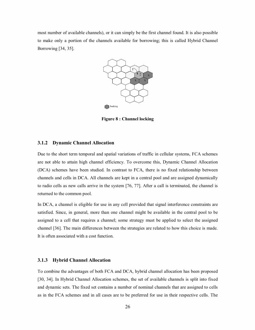
26
most number of available channels), or it can simply be the first channel found. It is also possible
to make only a portion of the channels available for borrowing; this is called Hybrid Channel
Borrowing [34, 35].
Figure 8 : Channel locking
3.1.2 Dynamic Channel Allocation
Due to the short term temporal and spatial variations of traffic in cellular systems, FCA schemes
are not able to attain high channel efficiency. To overcome this, Dynamic Channel Allocation
(DCA) schemes have been studied. In contrast to FCA, there is no fixed relationship between
channels and cells in DCA. All channels are kept in a central pool and are assigned dynamically
to radio cells as new calls arrive in the system [76, 77]. After a call is terminated, the channel is
returned to the common pool.
In DCA, a channel is eligible for use in any cell provided that signal interference constraints are
satisfied. Since, in general, more than one channel might be available in the central pool to be
assigned to a cell that requires a channel; some strategy must be applied to select the assigned
channel [36]. The main differences between the strategies are related to how this choice is made.
It is often associated with a cost function.
3.1.3 Hybrid Channel Allocation
To combine the advantages of both FCA and DCA, hybrid channel allocation has been proposed
[30, 34]. In Hybrid Channel Allocation schemes, the set of available channels is split into fixed
and dynamic sets. The fixed set contains a number of nominal channels that are assigned to cells
as in the FCA schemes and in all cases are to be preferred for use in their respective cells. The
27
second set of channels is shared by all users in the system to increase flexibility. When a call
requires service from a cell where all of the associated nominal channels are busy, then a channel
from the dynamic set is assigned to the call. The dynamic set is managed by a DCA scheme.
3.2 Call Admission Control All the allocation schemes presented above did not take into account the effect of handoff calls in
the performance of the system. In general, call hand-off is caused by the degradation of the radio
link, either because there is some change in the environment, or because the user is moving and
needs to change base station to keep sufficient transmission power.
From the user point of view, it is more frustrating to lose a call that has already begun than to be
prevented from establishing a new call. The user welfare will consequently be increased if special
care is given to handoff calls; even if it increases the blocking probability of new calls. For this
reason, many call admission control schemes that manage the tradeoff between handoff and new
calls have been proposed, each of which tries to give priority to handoff calls. In this section, a
selection of existing schemes will be presented, starting with some simple handoff priority
schemes, and continuing with more sophisticated ones.
3.2.1 Simple CAC Schemes
3.2.1.1 Guard Channels
Among all the CAC schemes, the Guard Channel scheme is the nearest to a standard, since it is
used commonly for experiments and has been subject to numerous studies over the past two
decades [37-40]. The guard channel approach offers a generic means of increasing the chances of
handoff call success, simply by allocating a number of channels exclusively for them. Although it
is possible to decide statically which channels will be guard channels and which will not, the
general meaning of guard channel call admission control does not refer to the static case. On the
contrary, even if the number of guard channels is fixed, the channels themselves are not.
What it means is that, if there are N channels of communication in the cell from which G are
guard channels, a new call will be accepted only if the number of available channels is superior to
G, whereas hand-off calls will be accepted as long as at least one channel is available.

28
The number of guard channels for a given network is extremely important. It is very easy to
understand how this parameter impacts on the overall performance. If all channels are guard
channels, it is impossible to start a new call, but the probability that a handoff call will be blocked
is very low. In the opposite case, if no channel is allocated exclusively for handoff calls, both
types of calls will be treated equally, neglecting the relative importance of the handoff calls. In
[41], the number of guard channels is adjusted automatically in real time to minimize the loss
probability of handoff calls, so that the trade-off problem is solved automatically.
3.2.1.2 Queuing Schemes
Along with guard channels, the queuing of calls is the second major scheme for handoff
prioritization. Different queuing schemes exist.
3.2.1.2.1 Queuing of handoff calls
This has been studied in [43]. The handoff calls are queued and no new calls are handled before
the handoff calls in the queue are. Hence, this is a stricter scheme than the guard channel ones.
The handoff calls can be queued because of the overlapping zone where two or more base stations
in neighbouring cells can work at the same time. Of course, it is not possible for a call to wait
indefinitely; it is necessary to impose a time limit, which will have been determined by analysis
of the average time that users stay in the overlapping area. Because the size of the buffers for
queuing is limited, handoff calls can be blocked before being queued.
3.2.1.2.2 Queuing of new calls
It seems more natural to queue new calls given the fact that they are almost insensitive to delay.
In [42], a method was proposed which involved the introduction of guard channels and the
queuing of new calls. The results showed that the blocking of handoff calls decreases much faster
than the queuing probability of new calls increases.

29
3.2.1.2.3 Queuing of both types of calls
It is also possible to queue both types of calls, and then decide to give a higher probability of
service to the handoff calls present in the queue.
Of course, to achieve better performance, the guard channel schemes and queuing schemes can be
combined [44, 45]. However, it is important to bear in mind that the more complex and efficient a
scheme is, the more computational power and time it requires to be applied. In the next section,
examples of very complex CAC schemes are presented, taking into account the mobility of the
users to adapt in real-time to the environment.
3.2.1.3 New calls bounding scheme
As mentioned previously, each CAC scheme suffers when congestion occurs, because it is not
possible to maintain both the new call and the handoff call blocking probabilities at a low level
when the number of incoming calls increases dramatically. A very powerful scheme would be to
avoid too many incoming calls. Because new calls in a cell are likely to become hand-off calls in
the neighbouring cells, it seems a good idea to restrict the number of new calls in a cell, to avoid
future congestion in its neighbouring cells.
In [46], this concept is used. The presented scheme works as follows:
{ newusedbndusednew BCBNBotherwisenewP −≤≤= &1
0
where :
- usednewB is the number of channels that is used by new calls.
- bndN is a given bound for new calls.
- usedB is the number of channels currently used.
- newB is the number of channels required by the incoming new call.

30
3.2.2 Advanced CAC Schemes
All the schemes presented in the previous sections were basic in the sense that they did not
consider the mobility of the user. Information theory shows that it is theoretically possible to get
better results by using mobility information in addition to traffic information. Therefore, the
majority of the schemes presented in this section are improvements on previous ones, but use
either guard channels or queuing as a basis.
One of the major advantages provided by mobility information over traditional CAC schemes is
“channel-reservation”. The concept is simple: if you can inform a cell that you will require one of
its channels at a precise moment of time, the target cell can do its utmost to ensure that this
channel will be available for you when you arrive. However, because channel-reservation is a
waste of resource (a reserved-channel remains idle until the arrival of the call), an efficient
reservation-based scheme should make the reservation at the latest possible moment. So it is
necessary to have the most accurate possible knowledge on when the call is to arrive, and
consequently, when the reservation is to be made. This precise knowledge is not easy to obtain in
real systems, because complete user behaviour is unpredictable. Nevertheless, a complete
knowledge is not necessary. The study of the reception power from different base stations, the
analysis of the user population mobility pattern or of GPS information are many different ways of
obtaining user behaviour information which have been studied in the literature.
In the following, a set of interesting proposals is discussed. These provide an overview of how
different strategies relating to mobility information can be used to improve the reservation of
resources for CAC schemes.
3.2.2.1 Influence curves
In [46], the mathematical concept of influence curves is introduced to take the mobility pattern
into consideration. It is based on the following observations:
- A user is more likely to request a handoff in the far future than in the near future once he
enters a cell. This implies that the handoff probability (the probability that a call needs at
least one handoff during remaining call life) is a function of the time elapses after a call
enters a cell.

31
- After dwelling in a cell for the same length of time, a high-speed user (for example a user
in a car) is more likely to request a handoff than a low-speed user (a pedestrian) is, which
implies that the handoff probability is also related to the speed class of a user.
Because of call hand-off, the traffic in different cells is no longer independent. A call in a cell not
only uses a channel in this cell, but also exerts an influence on the neighbouring cells (with
different probabilities), because it is likely to hand-off to one of those cells in the future.
From the aforementioned observations it can be concluded that the extent of such influence can
be characterized by both the elapsed time and velocity class.
If )(tf h and )(tf l represent the cell-dwell-time probability density functions of the high-speed
users and the low-speed users, respectively, the probability that a high-speed user entering a cell
will require a hand-off after time T is:
∫−
=tT
hh dfTtL0
).(),( ττ
Similarly, we can obtain ).,( TtLl Let ji,α be the directional factor, i.e., the probability that the
hand-off target cell is cell j when the call is being served in cell i. If no further information is
available, all the factors will be equal to 1/6. Of course, in particular places, the factor can be
different; for example this is the case on motorways, where all users on one side go into the same
direction.
The influence curve characterizing the influence exerted on cell j at time T by an ongoing high-
speed call which enters the cell i at time T is:
),(),,,( , TtLTtjiI hjiα=
Using the influence curve for every ongoing call, we can further determine the number of
channels it is necessary to reserve in each cell, as a portion of the total influence, this latter being
the sum of the influence curve for all ongoing calls in cell i.

32
3.2.2.2 Shadow cluster
In [47], the famous notion of Shadow cluster for channel reservation is introduced. This is a
general concept, which can be exploited at different levels given the degree of information
available regarding the users mobility.
It can be represented as in figure 9 below. The shadow is stronger where more reservations need
to be made, that is in the neighbouring cells which the mobile station is the most likely to move
into, according to its current mobility. In the cells in the path of the mobile station, reservations
can be made to a lesser extent, even in the cells which are not directly in contact with the current
one.
When the mobile station moves, its shadow moves as well, the resources reservations and
cancellations being made in real-time.
The base station of a cell is responsible for informing other base stations of the probability that a
mobile station under its control will require one of their channels in the future. Given this
probability, the target base station can decide whether to actually reserve a channel or not.
Figure 9 : Shadow cluster
3.2.2.3 Predictive Channel Reservation
The position of the mobile station in the network is also used in [48], where the notion of
“threshold distance” is used to define the size of channel reservation area. The PCR scheme
makes predictive channel reservations for each mobile station (MS) based on its current position
(calculated with GPS data) and orientation. The threshold distance is defined as the radius of a
circle which is co-centered with a cell, and this circle is smaller than the cell’s coverage area

33
(Figure 10 below). The area between these two circles is called the channel reservation area.
When a mobile station enters the reservation area of a cell from the inner part of that cell, and at
the same time, is heading to a new cell, a reservation request will be sent to that new cell’s base
station.
Figure 10 : Notion of threshold distance
3.2.2.4 Adaptive Channel Reservation
In [49], it is argued that the Predictive Channel Reservation scheme has some problems, including
the following: the threshold distance is the same for all users, regardless of their speed. Hence,
the time the base station will have to make the reservations can vary a lot between two different
incoming calls. Another problem can be seen in figure 10, where the mobile station in the
reservation area of the cell A, is heading to cell C. Although a reservation is requested, there is a
lot of time before the mobile station will actually enter into the cell C, which means that the
resource will be idle for a long time. This results in an under-utilization of the wireless resources,
which is to be absolutely avoided.
To overcome this, the Adaptive Channel Reservation scheme is introduced. This is not based on a
threshold distance, but rather on a constant threshold time thT . According to each mobile station’s
current moving speed, orientation and location information, base stations can predict the time
within which the mobile station will reach the boundary of its next target cell. This is represented
in figure 11 below, where the mobile station is moving with velocity V towards cell A. The
velocity V can be decomposed into two orthogonal component vectors, 1V and 2V , where 1V is
the velocity component of this mobile station towards the centre of cell A. From 1V and MSR

34
(the distance between the mobile station and the centre of cell A), we can estimate the time T by
which the mobile station will reach the boundary of cell A by:
1VRR
T CMS −= where CR is the radius of the cell.
Knowing T and thT , it is possible to make the decision on whether or not it is necessary to make a
reservation.
Figure 11 : Adaptive channel reservation
3.3 Conclusion In this chapter, some of the existing schemes for channel allocation and call admission control
have been presented. As the more advanced schemes, which use GPS data, mature, they may be
increasingly used in the future as mobile terminal technology progresses. The goal of call
admission control is to balance the trade-off between the new and handoff call blocking
probabilities, and it has consequently a great impact on user utility. Call Admission Control and
dynamic pricing have almost the same goal, and as shown in [7], their combined effect can be
even more efficient. For this reason, it seems particularly interesting to look at the effect of
different schemes in a dynamically priced mobile network. This is one of the objectives of this
project.

35
Chapter 4
GSM/GPRS Network Modelling
This project mainly focuses on analyzing the effects of different call admission control and
channel assignment schemes on a dynamically priced GSM/GPRS network. However, it is also
one of its objectives to continue the work started in [50], where a simulator for GSM/GPRS
network was built. In particular, the GPRS traffic model needs to be extended to be more realistic
and to take account of different types of applications: Web traffic, E-mail and file transfers.
In this chapter, a quick recapitulation of the GSM [51] and GPRS [52] technologies and how they
interact will be given, so that the experimental settings which will be used in the following may
be justified. It is not intended to provide a very detailed description of GSM and GPRS; these are
very complicated technologies and would require much deeper exposition than is possible in this
dissertation. Finally, existing proposals for GSM and GPRS traffic modelling will be presented
along with the choices made for this project.
4.1 GSM and GPRS Technologies
4.1.1 GSM
The origin of the “Global System for Mobile communications” (GSM) goes back to the year
1982. At that time, the European countries decided to develop and adopt a common norm for the
passage from analog cellular networks to digital technologies. The digital technologies are more
efficient than analog ones in their use of the spectrum; they can also offer more functionality and
security.
4.1.1.1 Concept of cellular networks
GSM, as in other radio telephony systems, uses a radio link between the phone network and the
mobile terminals. The transmission between these two entities must be of sufficient quality; this
is why a number of base stations (transmitters) have to be installed at different places in order to
cover the entire network area. The notion of cell, and thus of cellular networks, appears with
these base stations. A cell is the area where a mobile phone can establish a connection with a
particular base station. They are often represented by hexagons, because a hexagon is a good

36
shape to regularly cover a whole area, but they don’t actually have that form. Indeed, in reality,
the shape of a cell is more of an irregular circle, the irregularities being due to the obstacles
around the base stations, buildings for example. The size of the cell depends on the transmission
power of the base station. Huge cells are used in rural zones, whereas smaller cells are used in
city centres. As will be explained below, the number of frequencies allocated to GSM is
restricted. For this reason, they have to be reused among cells to increase capacity, which results
in networks with similar aspects to the one presented in figure 7. The number of cells using all the
available frequency band is called a cluster. Frequent clusters have 4, 7, 12 or 21 cells.
4.1.1.2 GSM frequencies sharing
Two frequency bands of 25 MHz have been allocated for the GSM system in the 900 MHz
frequency band. They correspond to the downlink and uplink. Each communication channel is
200 kHz wide and it is thus possible to split the available bandwidth into 125 duplex links.
However, only 124 are effectively usable, since the 125th channel is used for signalling. The
number of channels then must be equally shared among the phone operators.
In addition to the frequency multiplexing presented above (FDMA), temporal multiplexing
(TDMA) is also used to increase the capacity of GSM links. Each channel is divided into eight
time slots, and each user is only given one time slot for its communication. It means that each
user can only use the link for one eighth of the time.
Considering all the information mentioned above, a cluster of seven cells and three operators, it is
possible to give a rough calculation of the number of calls N that can simultaneously happen in a
cell:
473*78*124 ≈=N
This is the value that will be used in the simulator for the number of channels inside each cell.
4.1.2 GPRS
The tremendous growth in demand for mobile communications has very quickly shown the
limitations of GSM in face of the ever increasing amount of data to be transmitted. One of the
major reasons is that GSM is a circuit-orientated technology, which means that once a call is

37
established, one channel is exclusively allocated for this communication for its full duration, even
when neither of the correspondents is talking. This results in a very poor utilization of the
bandwidth.
To overcome this, the General Packet Radio Service using a packet-based technology was
introduced, reusing the GSM infrastructures. With GPRS, it is possible to achieve much better
throughput than GSM and better resource utilization. Indeed, a user only uses the link when he
really needs to, and releases it automatically as soon as possible. As a consequence, GPRS is
suitable for more types of applications, such as file transfer or web-traffic.
Unlike GSM, more than one time slot can be allocated for one call in GPRS (up to eight), which
explains why the maximum theoretical throughput is so high.
Because the bottleneck is the radio interface, new coding schemes for the radio channel have been
found, increasing the throughput from 13.4 to 21.4 kbits/s. These results are illustrated in figure
12 below [53], which represents the different throughputs (in kbits/s) at different layers of the
stack.
Figure 12 : Throughputs for GPRS in kbits/s
Because one user can be given eight time slots, each of them corresponding to a maximum
throughput of 21.4 kbits/s, the global maximum throughput that can be achieved is 171.2 kbits/s.
However, this theoretical value is almost never reached in the reality. The reason is that it would
require that a particular user gets the eight time slots available, which is possible only when the
network is not congested. Moreover, even if GPRS technology can manage up to eight time slots,
current mobile phones can not. Most of them can only manage four time slots for the downlink
and one time slot for the uplink. They are also limited in the sense that they often don’t use the
highest coding schemes (CS-3 and CS-4), which are too prone to errors.

38
Therefore, for this project, we will only consider the allocation of one to four time slots
(corresponding to one to four channels) for each call, and a throughput of 10 kbits/s for each
channel, which is a common value used in the literature.
4.1.3 Resources allocations between GSM and GPRS
Because GSM and GPRS calls share the same resources, there is a need to manage the way they
can have access to these resources. Because voice calls (GSM) are supposed to be more important
than data calls, the problem is very similar to the one with new calls and hand-off calls, which
was discussed in chapter 3. The same strategies can be adapted to this problem, for example the
queuing of the two types of calls with or without priority. Similarly, channels can be specifically
allocated for GPRS, or on the contrary the allocation can be made dynamically.
In [54], another scheme is presented. It is call “Dynamic Channel Stealing” and permits a GPRS
call to temporarily use the channel allocated to an inactive voice call.
4.2 Cellular Network Modelling The different strategies employed in the literature to represent a cellular network are now
presented. Because the results depend on this representation, it is a crucial parameter which needs
to be considered seriously. The problem is that it is not realistically feasible to simulate a full
network, since it would require a huge amount of computational power. It is thus necessary to use
a smaller representation, which keeps the salient characteristics of a global one.
4.2.1 Basic Approach
The basic approach consists of considering only one cell, and to model the arrival of handoff calls
using a mathematical formula. In [55], this solution is used and the following handoff call traffic
model is proposed:
inhb
nbh P
P ληµ
ηλ ..
)1.(+
−=

39
where
- hλ is the hand-off call arrival rate,
- inλ is the new call arrival rate in the admission block,
- nbP is the new call blocking probability in the admission block,
- hbP is the hand-off call blocking probability in the admission block,
- 1/η is the mean cell dwell time,
- 1/µ is the mean call holding time.
4.2.2 Classic Approach
The classic approach is to define a scenario consisting of a cell surrounded by one or, preferably,
two rings of interfering cells [56, 57]. With this representation, statistics can only be collected for
the central cell, since the other cell are not surrounded by the same number of cells and
consequently do not suffer from the same interference. This means that only 1/19 or about 5% (in
the case of two rings) of the simulation results are used. It represents an important loss of data,
which has to be avoided, even if the results obtained for the central cell are satisfactory.
4.2.3 Refined Approaches
In [58, 59], another approach is proposed. Because the problem with previous approaches was
that the data collected for the border cells was useless, the strategy is to get rid of these cells. In
order to achieve this, the so called “wrap-around” scenarios have been proposed. There are two
ways to represent it. The first is given in figure 13, the second in figure 14. In figure 13, the cells
simply continue on the other side of the map. In figure 14, it can be compared to a foot ball,
where cells are bound to each other, resulting in a sphere.

40
Figure 13 : Refined approach model 1
Figure 14 : Refined approach model 2
In [50], experiments were made to compare the results obtained using the last approach and the
first one. It showed that both approaches produce similar results. For this reason, it was argued
that it was not necessary to use a wrap around model with a large number of cells.
Therefore, for this project, a wrap around model consisting of seven cells will be used.
4.3 Traffic Modelling This section aims to justify the GSM and GPRS traffic models chosen for this study. For this
purpose, a brief overview of some existing proposals will be presented [60]. In particular
attention will be given to empirical measurements rather than purely theoretical studies.

41
4.3.1 GSM
The behaviour of voice users has been widely studied in the past. Traditional phone users and
mobile phone users have the same characteristics; it is hence possible to transfer the well-known
results from the first technology to the second. Indeed, in both cases, the communication
comprises a sequence of active phases (when the user is actually talking) and inactive phases
(when he is listening to his counterpart). For this reason, the traffic generated by these users is
usually characterized by an ON/OFF process. The only relevant parameters for this type of traffic
are the mean inter-arrival time between consecutive connections, and the mean connection
duration. It is widely accepted that exponential distributions should be used for both parameters,
resulting in a Poisson process description for voice users.
This standard will be adopted for this project, the arrival of GSM calls being represented by a
Poisson Process. The call arrival time is varied with the time of the day, as given in figure 15
below.
Figure 15 : Incoming traffic as a function of the time of day
4.3.2 GPRS
Although the modelling of GSM traffic is rather straightforward, the traffic generated by GPRS is
highly dependent on the application involved. Because most of these applications have a high
burstiness, the simple Poisson process description is no longer sufficient. Before giving more
details about how the different applications are represented, it is necessary to look at which
applications need realistically be considered for mobile phones. Vicari [61] investigated the

42
behaviour of dial-in users. Figure 16 below shows the traffic share of the most important
applications for access speeds between 9.6 kbits/s and 64 kbits/s.
Figure 16 : Traffic repartition for dial-in users
As mentioned in the previous section, the throughput experienced by GPRS traffic can change
with network congestion. However, the average current throughput is around 30 kbits/s.
Therefore, it seems relevant to use the results obtained for 33.6 kbits/s. At that throughput, the
principal traffic is web based, while other relevant applications are E-mail and File transfer. The
other applications each occupy a very small part and consist of games, telnet, etc., which are only
relevant for dial-in users but are not applicable to GPRS.
For this project, the GPRS traffic will therefore be made up of the following: 80% Web, 15% E-
mail and 5 % file transfer. A small readjustment had to be made to adapt the results obtained by
Vicari to GPRS (removal of other traffic types). The use of these applications is interesting
because they correspond to three types of applications: interactive, best-effort and background,
respectively [13].
4.3.2.1 Web Traffic
4.3.2.1.1 Measurement based proposals
Nowadays, the Web is the most important application used by the Internet community, and many
attempts to model its traffic have been proposed in the past decade. A web document is made of
HTML code (the main object) and additional other objects such as images or java code (inline
objects). For the transfer to be completed, every object has to be downloaded. Recent versions of
web browsers allow a user to download several objects simultaneously, by establishing multiple
connections. However, for this project, we will consider that all objects are downloaded

43
individually. It seems a more realistic view of web traffic for GPRS, which has to operate in a
wireless environment with a more restricted spectrum than typical wire lines.
There are three main ways to get information about web traffic. The first is the analysis of server
logs, which has been used in [62]. This does not permit the establishment of a model for a single
user so it is not relevant for this study. The second method is the analysis of client logs, used in
[63, 64]. Even if the results are relevant, the studies are of sufficient age that their reliability is
questionable. Packet traces are the main method that is almost always used today [65-69]: the
analysis of packets gives information about the application in use, from which it is possible to
deduce an appropriate model.
The different studies of the third type mentioned above can be separated into two categories. The
first type [67, 68] separates the traces into sessions and sub-sessions and proposes distributions
for both the inter-arrival times of sessions and the duration of a session. The others only consider
an unlimited session. The main studies of both types will be presented below.
In [67], a subsession is described as the time period during which a user actively uses the Internet.
Vicari found that a typical subsession is made of 19.6 web pages on average, each of them
consisting of four objects on average. The size of the global web document and the time between
web requests are modelled by Pareto distributions.
In [68], a more detailed model is provided, consisting of three levels, the session level, the page
level, and the packet level. The session inter-arrival time is then modelled by a Poisson process,
whereas the number of pages downloaded per session is represented by a lognormal distribution.
Page size is found to be Pareto distributed. The reading time between two consecutive sessions is
said to be Gamma distributed (mean 30s, standard deviation 140s).
Among the models using an ON/OFF process, the studies carried out by Deng in [65], by Mah in
[66] and by Choi and Limb in [69] are the most interesting ones.
Deng considered the simplest ON/OFF model, where the ON phase is the time during the
download processes and the OFF phase is the “viewing time” of the downloaded document.
Distributions for the three main parameters (duration of the ON period, duration of the OFF
period and inter-arrival time of web requests during the ON phase) were found, respectively
Pareto for the first and Weibull for the others.

44
Mah’s model is a little more sophisticated, since his OFF period is not only the time a user views
the downloaded page, but also the time between two sessions. The major advantage of this study
over the previous one is that Mah gives distributions for the size of objects in the web page.
However, their number is only given via median and mean, which are not easily used for
simulation studies.
Finally, the model presented in [69] is the most interesting. It is represented in Figure 17 below.
As can be seen in this figure, three different layers are considered. The ON/OFF model
corresponds to the arrival of web requests. The OFF time is said to be Weibull distributed
whereas the ON time depends on the size of the document to download. A division of the
document into one main and several inline documents is used. The object sizes are found to be
lognormal distributed (mean 10 kB and 7.7 kB), and the number of inline objects is found to be
gamma distributed (mean 5.5). Choi and Limb considered the recent versions of web-browsers
where several connections can be established simultaneously.
Figure 17 : Model of Choi and Limb for Web traffic
4.3.2.1.2 Models proposed by standards
All the models presented in the previous sections are based on actual measurements. In contrast,
the Web-traffic models proposed for UMTS [70] and cdma2000 [71] are only theoretical but are
recommended for performance analysis. For example, in [70], the page size is represented using a

45
truncated Pareto distribution and the number of pages per session by a Geometric distribution of
mean 5. The inter-session time is represented using a Poisson process, and the viewing time using
a Geometric distribution of mean 412 s.
4.3.2.1.3 Model used for this project
As far as possible, it has been decided for this project to use empirical values for the different
important parameters of Web-traffic. Among the different studies presented, the one made by
Choi and Limb is the most relevant. Therefore, the results presented in [69] will be used.
However, because some required parameters are missing in this study, the number of pages per
session and the inter-session time will be taken from the UMTS recommendation.
A recapitulation of the GPRS Web-traffic model is given in table 1 below.
Parameter Distribution Literature
source
Main object size
Lognormal
mean 10 kB
stddev 25 kB
Choi and Limb
Inline object size
Lognormal
mean 7.7 kB.
stddev 126 kB
Choi and Limb
Number of inline objects
Gamma
mean 5.5
stddev 11.4
Choi and Limb
Viewing time
Gamma
mean 30s
stddev 140s
Reyes
Inter-session time Poisson arrival process UMTS
Number of pages per session
Geometric
mean 5 UMTS
Table 1 : Model used for Web Traffic

46
4.3.2.2 Email and file transfer traffic modelling
Although web-traffic is made up of a sequence of sessions, where a user downloads a document
and then reads it, E-Mail and file transfer traffic is different. These only consist of one “session”,
where the user sends the file he has to send. The only difference between the two types of traffic
is the size of the file to transmit.
4.3.2.2.1 E-Mail
The number of studies concerning E-Mail traffic [60, 72-74] is much smaller than for Web-
traffic.
In [73], the analysis of a sample of 1760 E-mails shows an average size of 77.9 kB with a
standard variation of 337.6 kB. In [60], the result of the analysis of the E-Mail collection of a
sample of users at the University of Würzburg is presented. The average E-Mail size is found to
be 22.7 kB with standard deviation of 200.3 kB. In [72], a different approach is given. The E-
mails, of size smaller than 300 bytes are considered to be errors and are not taken into account.
The minimum size for an E-Mail is hence 300 bytes. The remaining messages are separated into
two categories, each of which follows a lognormal distribution of mean 1.7 kB and 15.7 kB
respectively.
Finally, in [74], an attempt to model the E-Mail size using a Cauchy distribution is made. It is
defined by the following density function, with α = 0.8 and β = 1.0.
12
1..)(
−
−+=β
αβπ xxf
This results in a mean size of 2.7 kB with standard deviation of 17.7 kB.
As can be seen with the figures given above, there is no real common value for the E-Mail size
distribution. Nevertheless, the results in [74] and in [72] seems to underestimate their size

47
whereas it is overestimated in [73]. For this reason, the middle value found in [60] seems to be
the most appropriate.
Because imposing a smallest size seems to be a good idea, it has been decided to adopt the
following E-Mail representation for this project: The E-Mail size will follow a geometrical
distribution of mean 23 kB, with a smallest possible size of 300 bytes. This geometrical
distribution was used in [75] and produced valid results in that study.
4.3.2.2.2 File Transfer
The average size of the files transmitted by GPRS is very difficult to estimate. Two important
facts need to be taken into account. The first is that, given the low throughput of GPRS, important
files will not be sent using this medium. The second is that FTP transfer is very rare because of
the importance of HTTP file transfers. However, a study of the average size of file transferred
was made in [72] and it was found to have an average of 4 kB. This is about the size of a JPEG
image, and thus this value will be used in the simulator. The same decision was made in [75].
File transfer will be considered to follow a geometric distribution of mean 4 kB.
4.4 Call duration and cell dwell times The GSM call holding time (total call duration) and cell dwell time (time a mobile host stays in a
cell) are modelled using a geometrical distribution. Contrary to the study made in [8], they are
assumed to be dependent on the price. They are however independent of time. When a call is
generated, both its call holding time and cell dwell time are generated and the minimum of these
two is used to determine a suitable event trigger to associate with the call.
In this project, except where otherwise stated, the call duration is assumed to be exponentially
distributed with a duration decreasing with price:
)1.(4.0
00.)( p
p
ep−
= ττ

48
where 0τ is the call duration of a call following a constant distribution, and 0p is the normal
price.
4.5 Conclusion Along with a presentation of different GPRS traffic representations, this chapter has given the
different settings which will be used for the experiments carried out in this work. The choices
were made using the most relevant and appropriate results obtained by different studies. It should
be noted that in some cases the differences between similar studies were significant and, where
necessary, the average results have been used.

49
Chapter 5
Simulator
Given the complexity of the different pricing algorithms presented in chapter 2 , and the wide
variety of available call admission control schemes, the use of a simulator was considered a
necessity in order to achieve the goals of this project. Therefore, the simulator built for the work
presented in [50] has been used, improved and extended. The same developing tool (IntelliJ
IDEA 3.0.1) has been kept, so has the java programming language.
In this chapter, a description of the main characteristics of the simulator will be given along with
the improvements made and the new features added to it.
5.1 Design of the Simulator
5.1.1 Type of Simulator
The simulator is a discrete event, event-driven simulator. Discrete event means that the effects of
every particular event are taken into consideration, which is not the case in simulators where the
average effect of several combined events is used instead. Event-driven means that the simulator
clock advances from one event time to the next event time, and that there is no fixed time
increment.
This choice of simulator has repercussions on its performance, and also gives rise to inherent
limitations. Indeed, because it is a necessity to model every event, it is not possible to create an
unlimited number of them. For example, it is not realistically feasible to put an event in a queue
and to make it wait until another condition is fulfilled, with an expectation that it will stop waiting
as soon as the condition is fulfilled. That would require a huge number of similar events with very
close execution times in order to maintain the illusion of continuous time. As memory is limited,
this solution is to be avoided, and the simulation time has to be split into larger slots.
5.1.2 Level of Abstraction
The main goal of the simulator is to provide a computational aid for studying the influence of call
admission control and dynamic pricing in a GSM/GPRS network. The performance of GPRS

50
traffic is not a centre of interest here, so it is not necessary to track the behaviour of every packet.
It is sufficient to know how the system will behave at the call level, so this is the level of
abstraction which has been used.
5.1.3 Functioning of the Simulator
A simplified class diagram of the structure of the simulator is given in figure 18 below.
Figure 18 : Simplified class diagram
The main class is the class Simulator. An instance of Simulator is associated with an instance of
the Network class, which represents the set of cells used for the simulation. The number of Cells
to be generated in the network is given by the network size attribute, which is a simulation
parameter specified by the user.
One of the most important classes is the class Cell, representing one cell of the network. Each cell
manages its own set of channels (it integrates the call admission control block), calculates its own
revenue and utility, and updates its own dynamic pricing. When GPRS traffic is used, a number
of GPRSChannel instances are created for every cell and bound to them. The role and behaviour
of the GPRSChannel class will be explained later.
When the simulator is initialized, an EventList is created to manage the different events. The
events are stored and sorted by increasing execution times. When the simulation starts, the first

51
event is executed (by calling its execute () method) and removed from the list, and then the
second is handled, etc. The same process is repeated until the event list is empty or the next event
time is greater than the total simulation time. When the simulation is finished, the Output class is
used to average the results and to write them into text files, for later analysis.
The Random class is used to generate the event execution times, as well as the GPRS call
characteristics such as the number of sessions or the different reading times. Number-generation
functions following the different required distributions are available. The new distributions added
for this particular project use the same package as the previous ones (package cern.jet.random),
in order to maintain stability and to reduce the risks of small incompatibilities.
Another class of major importance is the Event class, since events are the basis of all event-driven
simulators. An event is bound to the cell where it has to execute. The Event class is an abstract
superclass. The event hierarchy is presented in figure 19 below.
Figure 19 : Event hierarchy
The two different types of events are EventStart and EventClose, which correspond to the start
and to the end of a GSM call or of a GPRS session. Because GSM calls and GPRS sessions do
not behave the same, it has been necessary to create different subclasses, resulting in the classes

52
EventStartGPRS, EventStartGSM, EventCloseGPRS and EventCloseGSM. In addition, in the case
of GPRS, the three considered types of sessions (Web session, File and Email) have their own
subclasses, as can be seen in the figure.
The initial EventStarts are created at the very beginning of the simulation. If GSM traffic is used,
one EventStartGSM is created for each cell. If GPRS traffic is used, a function from the Random
class is used to determine the type of the GPRS session, prior to the creation of the corresponding
EventStart. They are then put in queue in the EventList. When they are to be executed, their
getResource( ) method is called. This method will behave differently depending on whether the
event is a GSM call or a GPRS session. In the case of a GSM call, it will look at the number of
available channels (including the possible borrowing of a channel from another cell if this call
admission control scheme has been selected), and then decide to accept or to block the call
accordingly. In the case of a GPRS session, it will first make an attempt to get a number of
available channels (updating the channelsAllocated attribute of EventStartGPRS), which will be
between zero and four, zero corresponding to a blocked call. Then, the call characteristics will be
used in order to handle the call successfully, using the different channels got in the previous step.
This will be described briefly in the next section, when the GPRS traffic is considered.
When deciding whether a call is to be accepted or blocked, the cell also updates its own
characteristics, such as the number of accepted calls, the number of blocked calls for handoff and
new calls, and the total utility generated by the cell. Then, every five minutes, it uses those values
to update the price which will be used when the dynamic pricing function is activated.
5.2 GPRS Traffic
5.2.1 Introduction
As mentioned in chapter 4, GSM and GPRS traffic are fundamentally different. The simple
simulator model used for the GSM calls, where an available channel will remain available for the
whole call duration, can not be applied to GPRS sessions.
Another point of interest is the duration of a particular call, which is needed when the price is
based on the call duration. This is straightforward for GSM calls: the call duration is calculated
during the creation of the corresponding EventStartGSM event, and the price is computed when
the related EventCloseGSM event is executed. When GPRS sessions are considered, this is not
possible. Indeed, the call duration can not be known directly at the initialization of the call,

53
because it depends on the state of the GPRS channels. For example, the more congested a channel
is, the longer it will take to transmit a file.
The GPRS traffic model used in the simulator has been completely rewritten for this project,
mainly to facilitate multiplexing. In the new simulator, a call will release the channels it has
during the viewing times of a web session. During those times, the channels will be available for
use by other calls. This is not quite the real GPRS model, where the bookings of the channels are
managed in real time considering the different sessions happening at the same time, but it is
closer to reality than the model formerly used. It was not possible, given the limitations of the
chosen type of simulator, to implement the real model. This would have required calls to wait
until another call has finished transmitting, which, as mentioned previously, is not possible.
Instead, a simplified model has been used, which is presented below.
5.2.2 Representation of a GPRS Call
Three types of GPRS sessions have been considered for this project. However, it is possible to
use only one global representation. The callCharacteristics attribute of every EventStartGPRS
instance contains all the information about the call. Its representation inside the simulator is given
in figure 20 below.
The call type refers to “WEB”, “FILE” or “EMAIL”, whereas the type of first session is either
“SESSION”, or “VIEWING-TIME”. The number of pages is the number of web pages that the
web session will download when the call is a web session. This is set to one for emails and file
transfers. Finally, the sequence of sizes and viewing times depend on this number, but will always
finish by a size, since once the last page is downloaded, it is read after disconnecting from the
network.
Figure 20 : Representation of a GPRS call
Call Type Type of
first
session
Number
of pages
Size of
first page
Duration
of first
viewing-
time
Size of
second
page
Duration
of second
viewing
Time
Size of
third page

54
During the execution of the getResource() method for a GPRS call, a number of channels is
allocated to the call, then the callCharacteristics attribute is used in order to book the different
GPRSChannels. For this purpose, each GPRS channel owns a bookingTable attribute, which
represents a succession of one second time slots for the experiment duration. This means that the
duration of the call is second based. Even if a call would only require 0.2 seconds, the full second
will be booked, and thus paid for. When a GPRS call wants to book a channel, it has to deal with
different parameters. The first is that it may encounter partially booked channels where the
different channels may have been booked by other calls. The second is that it has to book the
different channels in parallel, since it would not be right to book one channel for nine seconds and
another for only two seconds. Finally, it has to respect the cell dwell time, which is the maximum
amount of time that the call can spend in the cell. In order to do that, it has to maintain the
callCharacteristics attribute so that it may be transmitted when the corresponding handoff call is
generated.
In this model, the priority is thus given to the first arriving call, since the next call will have to
cope with an already partially booked channel.
A simple example of the handling of a GPRS call is presented in figure 21 below. The call has
been given three different channels (represented by a row of the table) and is supposed to be a
web session with only two pages to download. The size of the first session is of nine time slots
duration followed by a viewing time of six seconds. The last session represents a transmission
time of six time slots. The upper part of the figure represents the states of the channels before the
handling of the call, and the lower part their states after.
busy free
Figure 21 : State of channels before and after GPRS call
55
We see that no changes are made during the six seconds of viewing time, and that the correct
number of time slots is reserved elsewhere.
5.3 Features of the Simulator The proposed simulator includes a number of different features, which makes it possible to carry
out a large range of experiments. First, the experiments can be realized in steady state or in real
traffic conditions. Then, different call admission control schemes can be selected (queuing of new
calls, queuing of handoff calls, guard channels schemes, channel borrowing with and without
locking, dynamic and hybrid channel allocation), individually or in combination. Finally,
different traffic parameters such as the GSM traffic-rate for the overall traffic, the proportion of
the different types of GPRS sessions, as well as the users’ behaviour can be defined.
The simulator can be used in two different modes, unicellular and multi-cellular. In the case of
the multi-cellular model, the size of the network can be specified. Although those two different
models require a completely different way of functioning, this is completely transparent to the
user.
All the different properties are regrouped in a java property file. During the execution, the
different properties are then loaded from this file and are provided to the classes as needed.
5.4 Simulator Validation The parts of the simulator built last year had been extensively tested to ensure their good
functioning. The same approach has been used for the new features. The validity of the different
statistical distribution has been verified before use. The GPRS traffic model has been tested on
simple test cases to ensure that it behaves as expected even for complicated situations. Before
launching the real experiments, simple ones have been carried out to ensure the coherence of the
results with what was expected. The unicellular model will not be used for this project,
nevertheless the concordance of its results with the other model has been checked.

56
5.5 Conclusion In this chapter, the main characteristics of the simulation tool used for this project have been
outlined. A brief description of how it behaves has been given, along with a presentation of its
features and its limitations. The model used for GPRS traffic has also been presented and
illustrated by a simple example. In the following chapter, different experiments about call
admission control and dynamic pricing are carried out using the simulator, and the statistics
generated are then analyzed and the results presented.

57
Chapter 6
Experiments and Results
This study has three objectives: to compare different simple call admission control schemes
(presented in chapter 3), to look at the impact of different factors which may influence the results
when GPRS traffic is included, and to look at the influence of dynamic pricing. In this section,
the simulator described in the previous chapter is used to carry out experiments. The results are
then presented and analyzed.
The experiments conducted fall into two distinct groups: one where dynamic pricing is not used
and the other where it is. The first represents the simple case, where nothing is done to regulate
the traffic. The second permits the exploration of the influence of dynamic pricing.
It has been decided to obtain two different types of results for each experiment pertaining to the
CAC schemes. First, the total revenue and utility generated during a day are needed for a direct
comparison of the schemes. But, since it would have been very restrictive to only use the
simulator for those two values, one or more additional metrics will be gathered for every case.
These will be explained individually in the following sections.
Every result presented is an average of at least fifty full-length simulation runs and of three
hundred simulation runs in most cases.
The utility and pricing functions used in the simulator are the ones mentioned earlier in this
dissertation, and the user behaviour has been set to the most elaborate case presented in [8], that
is to say the case where one third of the blocked users retry after twenty minutes and one third of
the users who find the proposed price too high retry after the same amount of time.
It should be noted that the unit used for the revenue is as follows: 100 corresponds to the price to
make a GSM call of duration one second.

58
6.1 Steady State
6.1.1 Experiment
To study the behaviour of the simulator in steady state is not exactly part of this project, but it is
very useful to get a better understanding of how it really works. Moreover, this experiment is a
prerequisite to all following experiments, since, as mentioned in chapter 2, the optimal arrival rate
is the crucial factor in the whole dynamic pricing strategy.
Thus, for every particular experiment, it is necessary to determine beforehand the corresponding *λ by performing one experiment in the steady state.
6.1.2 Results
The results obtained where there is no guard channel are given in the figure 22 below. The shape
of the graph is characteristic of this particular type of experiment. We see that in this case *λ is
found to be 0.13. For values of lambda smaller than 0.13, the increase of the utility is almost
linear, whereas this is no longer the case when lambda exceeds 0.13. This is understandable: for
λ< *λ , the network is under-utilized, so the rate of blocked calls remains quite small. Therefore, if
λ doubles, the number of accepted calls will almost double as well, and this will result in a double
of the total utility.
In contrast, as soon as λ starts to exceed *λ , there is congestion, the network can no longer cope
with the number of incoming calls. The level of congestion increases faster than λ, and the graph
is no longer linear.
Figure 22 : Utility as a function of time in the Steady State

59
6.2 Guard Channels
6.2.1 Experiment
As mentioned in the chapter 2, the guard channel scheme is the nearest call admission control
scheme to a standard. Its principle is simple: handoff calls have access to more channels than new
calls. It has also been mentioned above that one of the challenges is to establish the optimal
number of guard channels for the network. For this reason, this experiment aims to look at the
influence of N (the number of guard channels) on the total revenue and utility generated over a
day under the given experimental conditions.
6.2.2 Results
The variation of total utility and total revenue with N are presented in the two figures below
(figure 23 and 24). In each figure, both cases, with and without pricing are displayed
simultaneously.
What can be seen first is that both figures have similarities. Indeed, for both revenue and utility,
the two graphs decrease with N. It means that the loss of utility and revenue triggered by an
increase of N, when fewer new calls can be admitted, is higher than the corresponding gain due to
a lower loss rate of handoff calls. This first result may seem a little unexpected, since it suggests
that the presence of guard channels is not a good thing for the global results. However, one must
bear in mind that the guard channels scheme, as other call admission control schemes, has been
designed to cope with congestion. Even if it achieves its aims during periods of high congestion,
it is likely that its influence on a full day of traffic, with large amounts of time when the network
is not congested, can hardly be seen.
To validate this, another experiment has been carried out in steady state, with a constant value of
λ equal to 0.3, which corresponds to a moderate level of congestion. The results show that for this
value, the optimal value for N is 1 (N set to 2 also gives better results than when it is set to 0). It
is also very likely than it would have been higher for a greater value of λ. This is a good proof
that a network with guard channels performs well when there is congestion.
The second point of interest is the influence of pricing. As can be seen, it is different for revenue
then for utility. For utility, the growth is spectacular: the maximum grows from 1600 to 10500.
This means that dynamic pricing is very efficient in fulfilling its function as a regulator of

60
incoming traffic, resulting in really low rate of blocked calls, and thus a very high utility. On the
contrary, the revenue generated using dynamic pricing is lower than the one generated without it,
although both maxima are almost the same. This is not due to dynamic pricing itself, but it is due
to one experimental assumption: the call duration is said to be dependant upon the price, and it
decreases faster than the price increases.
Figure 23 : Revenue as a function of N
Figure 24 : Utility as a function of N
An additional experiment has been carried out. Instead of deciding on a fixed number of guard
channels at the beginning of the simulation, the simulator had to adapt this number to the traffic
conditions, in order to maintain a handoff call blocking probability below 0.005. With pricing, N
constantly remained equal to 0, which means than the limit value was never reached. It once
again shows the power of pricing as a traffic regulator. Without pricing, this is not the case and

61
the results are presented in figure 25 below. We see than the shape of the graph is very close to
the shape of the incoming traffic rate, with a maximum of 6.2 guard channels in average. At the
beginning and at the end of the day, N remains equal to 0 for a small period of time, because there
are so few incoming calls that there is no congestion at all.
Figure 25 : N as a function of time
6.2.3 Conclusion
This first set of experiments has shown two important results. The first is that the introduction of
pricing has very significant effects on the total utility, which is not a surprise when we recall that
the whole pricing strategy is intended to optimize it. The second important result is that under the
chosen experimental settings, it is preferable not to use any guard channels, since this triggers a
loss of revenue and of utility. Therefore, for the rest of the experiments, no guard channels will be
used.
6.3 Queuing Schemes
6.3.1 Experiment
In the previous section, the calls had only one opportunity to enter the system. If no resources
were available, they were immediately blocked. On the contrary, in this section, queues are
introduced. Three schemes are studied. In the first, new calls are queued: they are allowed to wait
in a buffer for twenty seconds and to make an attempt to enter every second. The second is the

62
equivalent for handoff calls, but they can only wait for ten seconds for a maximum of ten
connection attempts, since they are more sensitive to delay. The last one is the combination of the
queuing of both new calls and handoff calls.
In addition to total revenue and utility generated, the variation of the percentages of calls which
need to be queued with the time of day, and the average number of attempts required before
acceptance are also studied.
6.3.2 Results
Without pricing, the queuing of both gives a total utility of 4,733 and a total value of 3,429,149
for the revenue. The queuing of new calls gives a total utility of 14,766 and a value of 3,428,062
for the revenue. Finally, the queuing of handoff calls gives a total utility of 15748 for 3,421,141
of revenue.
With pricing, the values become, for utility and revenue respectively: 14,409 and 4,697,746 for
the queuing of both, 19,018 and 4,987,706 for the queuing of new calls and finally 18,021 and
4,955,562 for the queuing of handoff calls.
The first thing to notice is that the results obtained for the total utility are significantly higher than
the ones obtained without queuing. It would, of course, not be realistic to say that the queuing
schemes are much better than the guard channel ones. Indeed, the different figures are not directly
comparable, since it was obvious that with up to twenty tries for new calls for example, their
chance of being accepted was much higher than with only one attempt. In addition, this scheme
requires a more complex infrastructure, with the introduction of sufficiently large buffers and
with the management of the time spent queuing by the different calls.
The second is that it seems more efficient to queue only one type of calls than both of them. It is
not really difficult to understand why. When both types are queued, this results in a large queue,
with many new calls and handoff calls. Finally, the maximum time spent queuing excepted, it is
similar to the case of a system without a queuing scheme, but with a different incoming call rate
(which is higher but which has also not exactly the same shape with the time of the day). It also
seems preferable to queue handoff calls rather than new calls. This is due to the utility function,
where the loss of one handoff call is twice as important as the loss of a new call.

63
Concerning the revenue, the values are very similar to the ones obtained in the previous case,
which confirms the first idea that this is almost the maximum value without pricing, (around
3,500,000).
The introduction of pricing has again had a very positive effect. The utility increases
significantly, even if the growth is smaller than for the simple guard channels scheme, and is not
that far from the theoretical maximum (found to be 23,000 under these experimental settings).
The maximum is now obtained for the queuing of new calls, but the difference between this and
the value for the queuing of handoff is still small. The queuing of both call types gives much
better results with the introduction of pricing, even if it is still not as good as the others. The
revenue also increases significantly, to almost reach 5,000,000 (again not far from the maximum
of 5,200,000). This shows that the combination of a less restrictive admission scheme and traffic
regulation by dynamic pricing really is very effective.
The variation in the percentages of new and handoff calls which need to be queued (that is to say
which are not admitted at their first attempt) for the first two cases are presented in figure 26
below. The figure 27 represents the same characteristics for the queuing of both call types.
Figures 28 and 29 represent the average number of attempts before acceptance for the different
types of calls.
In figure 26, we can see that on average new calls are queued more often than handoff calls,
which can be explained easily because there are more new calls than handoff calls in the system.
What we see as well is that without pricing, the two graphs have a regular shape (with a
maximum of 65% for new calls and 32 % for handoff calls), which is not the case with pricing.
Indeed, in the latter case, the two graphs have two separate parts. In the first part, corresponding
to the beginning and to the end of the day, the results are almost the same as the ones without
pricing (because the pricing function is not activated yet). However, this is not true for the second
part, which corresponds to the middle of the day, where the pricing scheme has come into effect.
The graph stops increasing, to remain at a quite low level (around 10 to 20 %). We can also
notice than the differences between handoff and new calls have almost disappeared. The small
dissymmetry between the two spikes on the left and on the right is due to the difference in the call
duration. Before the first spike, there is no pricing, so the calls last in average longer than the
ones before the second spike, where the pricing scheme is active.

64
Figure 26 : Percentages of calls queued as a function of time
In figure 27, we can see that the four graphs can almost exactly be represented by two graphs
only. Indeed, because there is no difference between new and handoff calls with regard to the way
they are put into the queue, their relative graphs are extremely close. On the graph corresponding
to the case without pricing, we see that it has a regular shape, with a maximum of 65%. With
pricing, the values become almost equal to 0, while again two small spikes occur at the beginning
and at the end of the day.
Figure 27 : Percentages of calls being queued as a function of time 2

65
Figure 28 : Number of attempts before treatment as a function of time
In figure 28 above, representing the average number of attempts before connection in the cases of
the queuing of new calls and of handoff calls, we can see that the graphs almost look the same as
the ones representing the percentage of calls being queued. The comments made previously are
consequently, still appropriate. Nevertheless, there is one difference in the case without pricing,
where we see that the differences between new and handoff calls is much more significant in this
case.
In figure 29 below, we see that even if the curves corresponding to new calls and handoff calls
are similar, new calls make on average 2.5 attempts more than handoff. This is a consequence of
the difference in the maximum time spent in the queue by the two types of calls. However, as
soon as pricing is introduced, there is no more difference, and we see that almost all calls are
connected at the first attempt.
Figure 29 : Number of attempts before treatment as a function of time 2

66
6.3.3 Conclusion
The analysis of the different graphs presented above has shown that the introduction of a queuing
scheme can improve the performance of the system, at the expense of a more complex
infrastructure. The average number of attempts for the different schemes suggests that the limit of
twenty seconds in the queue for new calls is too high, and that ten seconds may have been
sufficient. The dynamic pricing also permits an increase in the revenue and the utility, but makes
the queues almost redundant. Moreover, the results are better when dynamic pricing is used in
addition to queuing rather than when it is used in isolation.
6.4 Channel Borrowing
6.4.1 Experiment
In the last section, we saw that the introduction of queuing has a positive effect on the total utility
and revenue generated. However, it is not possible to make a direct comparison with the simple
case where every call has only one chance to be accepted. In this section, this one-chance-only
property is reintroduced. The difference here is that when a cell has no channel left, it can try to
borrow one from one of its neighbouring cells.
In addition to utility and revenue, the number of channels borrowed and lent at different times of
the day is studied. Two different experiments have been carried out here. The first involves
simple channel borrowing without locking. The second introduces locking, which is necessary in
real systems to take the interferences generated by the calls into consideration.
6.4.2 Results
For utility and revenue, the results are as follows: without pricing, the experiment without locking
gives a utility of 2,118 and 3,981,648 for revenue. With pricing, those values become 13,144 and
4,338,099. When locking is considered, the experiment without pricing gives a utility of 1,332 for
2,862,247 of revenue. Those figures become 10,698 and 3,577,583 with pricing.
The introduction of channel borrowing permits a better utilization of the global resources of the
system, and it can be seen in the utility, which is better than in the simple case. The same is true
for the revenue, however it remains lower than in the queuing schemes case. The introduction of

67
locking has, as expected, had a very negative effect. As mentioned previously, the borrowing of
one channel leads to the loss of more than one channel due to interference. The results seem
coherent with this fact.
The number of channels borrowed and lent in the case of borrowing without locking is now
studied using figure 30 below.
Figure 30 : Number of channels borrowed and lent as a function of time
Without pricing, the two graphs have almost the same shape as the incoming call traffic. The
number of borrowed channels reaches a maximum of 175, whereas the number of lent channels is
never greater than 140. This result is surprising, because it would have been expected to see both
of those figures being equal. This is due to the overlapping model used for this experiment (only
seven cells are considered). Indeed, even if the central cell really has six different neighbours, this
is not the case for the other cells which only have four different ones.
As soon as pricing is introduced, it is no longer necessary to borrow channels from the other cells;
the cells’ own channels are sufficient to cope with the incoming traffic. The same spikes at the
beginning and at the end of the day can be observed, for the same reasons as before.
The case with locking is now presented in figure 31 below. The focus of interest here is the
differences between the number of locked and borrowed channels. Since the number of lent
channels is very close to the number of borrowed channels, it has not been shown. As expected,
the number of locked channels is always higher than the number of borrowed ones, which
explains the loss of utility and revenue. In a network without model restrictions, one graph would

68
have almost exactly been the double of the other. Another point of interest is to note that the two
graphs reach a plateau quite quickly and stay there for a long time.
With pricing, since it is not useful to borrow channels, it is thus not useful to lock ones, which
explains why both graphs always stay close to zero.
Figure 31 : Number of channels borrowed and locked as a function of time
6.4.3 Conclusion
Channel borrowing allows a cell to increase its number of channels when it really needs to, and to
lend one of its unused channels to other cells. As a consequence, more calls can be treated, and
the utility is higher. A really good study would have required a more accurate network model
than the simple overlapping model used here, but due to time restrictions it was not possible to
implement this. The introduction of locking has negative effects, but it is a necessary restriction
in real systems. The final thing to bear in mind is that with the model considered here, where the
traffic is homogenous among the different cells, channel borrowing is not as powerful as it is in
systems where some channels are much more loaded than others.

69
6.5 Dynamic and Hybrid Channel Assignment (DCA & HCA)
6.5.1 Experiment
The experiment presented in the section above used channel borrowing as a means to improve
utilization of the global resources of the network. In this section, we take another step in this
direction by incorporating dynamic and hybrid channel allocation, as introduced in chapter 3.
With dynamic channel allocation, there is no channel assigned specifically to one call, but rather
a pool of channels available for sharing among the different cells. When one cell needs to use a
channel, it just takes one from the pool if it is available and then gives it back when the call is
finished. Hybrid channel allocation is a combination of fixed and dynamic channel allocation. For
the DCA experiment, a pool of 329 channels has been used (corresponding to 47 * 7), whereas
for the HCA, the pool had a size of 161 channels for 24 channels left in each cell (this
corresponds to 50 % of the total number of channels of the system available in the pool).
6.5.2 Results
The dynamic channel assignment scheme used without pricing gives a total utility of 1,762 for
3,600,402 of revenue; the figures become 12,655 and 4,192,565 with pricing. The hybrid channel
assignment gives 1,816 and 3,490,733 without pricing and 12,696 and 4,196,586 with.
The general result observed for pricing is verified once again: it increases both utility and
revenue, and it makes the different call admission control schemes (here DCA and FCA) almost
identical. Without pricing, we see that hybrid channel assignment gives a better utility but creates
a little less revenue than dynamic channel assignment. Finally, even the HCA scheme does not
give as good results as the channel borrowing scheme. This can be understood quite easily: in the
case of channel borrowing, the results presented earlier showed that the average number of
borrowed channels was higher than the average number of lent ones, which results in an overall
increase of the total number of channels, becoming on average higher than 47. As a consequence,
more calls could be handled. With DCA and HCA, the division is made equally, resulting in an
average number of exactly 47 channels. Moreover, in the case of HCA, a cell can not have less
than 24 channels, which is not the case for the DCA.

70
Figure 32 : Number of channels in pool as a function of time
The variation of the number of available channels in the pool for HCA and DCA, with and
without pricing, is presented in figure 32 above. The results are similar for the two schemes.
Without pricing, the number of available channels decreases regularly from the origin to zero,
where it stays for most of the day, which means that there is congestion and that all channels are
needed. We can see however, that for HCA, this number remains constant and equal to 161 for a
short period of time at the beginning and at the end of the day. This corresponds to periods with
very low incoming traffic, where the 23 channels assigned to each cell are enough to cope with all
incoming calls, without having to request a channel from the dynamic pool.
With pricing, the behaviour of the system is comparable to that which we saw for the previous
experiments. During the periods where there is no congestion, when the pricing has not come into
effect, it behaves exactly as in the experiment without pricing, but it never reaches zero. Indeed,
when congestion occurs, the price starts to regulate the traffic, resulting in less new incoming
calls. All channels don’t need to be used at the same time anymore, and so the number of
available channels starts to increase. The number of available channels is at its maximum at the
middle of the day, where the price is at its highest, which is what was expected. At the end of the
day, there is no more congestion, the pricing stops, and the graph starts to follow the one of the
case without pricing again.
A complementary metric has been considered in the case of HCA: the proportion of calls which
have been treated using the channels in the dynamic pool (presented in figure 33 below). Without
pricing we see that this number, after having stayed for a while at zero when there is no
congestion, increases regularly until it reaches the value of 50%. This is logical when we recall

71
that there are 50 % of the channels in the pool. At the end of the day, the behaviour is the
opposite; it decreases to zero again, where it stays for almost the same duration.
With pricing, this percentage never reaches 50 %, because as soon as it reaches 45 %, the pricing
scheme makes it decrease to a final value of 18%, before it starts to increase again to 35%, until
the pricing stops, triggering the channels in the pool to be increasingly less used.
Figure 33 : % of calls using channels in pool as a function of time
6.5.3 Conclusion
Dynamic channel assignment represents a good improvement on the basic system, but it is not as
efficient as channel borrowing. When pricing is introduced, the performances are again
significantly increased, and all channels are not used at the same time. This allows the system to
ensure that there will always be one channel available for an incoming call, new or handoff, and
this leads to the optimization of the utility.
6.6 Conclusion About the Experiments Carried Out Considering GSM Only The table below summarizes the values obtained for the utility and for the revenue for the
different experiments presented above.

72
Table 2 : Results for the experiments carried out with GSM only
In this table, what is remarkable is that the introduction of pricing always has a positive effect on
the total utility, and almost always on the total revenue. However, it is always the total utility that
is considerably increased. The best results with and without pricing are always obtained by the
queuing schemes, which is not surprising as mentioned above. We see that the channel borrowing
without locking also gives good results.
Another point of interest is to notice that the different schemes studied are very efficient at
improving the utility, in which they are all (channel borrowing with locking excepted), better than
the simple case, but they don’t improve the revenue significantly when there is no pricing. This is
due to a simple fact: the maximum theoretical revenue is obtained when all the channels are
always busy, which requires a good resource management. Since traditional CAC schemes can
not cope with congestion efficiently, the resource utilization is not maximized when there is no
Scheme Utility no Revenue no Utility yes Revenue yes
0 Guard Channel 1,600 3,450,000 10,500 3,450,000
Queuing of New
calls 14,766 3,428,062 19,018 4,987,706
Queuing of
Handoff calls 15,748 3,421,141 18,021 4,955,562
Queuing of both 4,733 3,429,149 14,409 4,697,746
Channel
Borrowing
without locking 2,118 3,981,648 13,144 4,338,099
Channel
Borrowing
with locking 1,332 2,862,247 10,698 3,577,583
DCA 1,762 3,600,402 12,655 4,192,565
HCA 1,816 3,490,733 12,696 4,196,586
73
pricing. However, when the pricing is used to make the traffic smoother, they start to become
very efficient and succeed in increasing the total revenue as well.
Two final experiments have been carried out, to see whether or not it is possible to get better
results than the ones obtained by the queuing of new calls and handoff calls.
First, the combination of handoff call queuing and channel borrowing gives a utility of 19,819
and 3,976,704 for revenue. In this case, it was not necessary to introduce pricing, since the
optimal value found for lambda was higher than the maximal arrival rate of 0.45 calls per second.
The utility is the best obtained so far, but this is not the case for the revenue.
Next, the combination of handoff call queuing and HCA has been studied. Without pricing, the
results give a utility of 17,615 and revenue 3,485,772; these figures become 19,251 and 4,522,484
with pricing. The results are better than the ones obtained without combination, but not as good as
when using the combination of channel borrowing and handoff call queuing.
Finally, it seems possible to improve upon the best utility obtained in the experiments presented
above, but only at the cost of introducing a more complex scheme. This is a general observation:
in order to get good results, very elaborate schemes have to be applied. Pricing, however, does
not really respect this rule: it is very simple, does not require more infrastructure, but gives
excellent results. Its effect on incoming traffic makes it possible to cope with every traffic type,
even in highly congested periods.
All results obtained for dynamic and hybrid channel assignment, and for channel borrowing, are
for the simplified model used for the network by the simulator. Further refinement of this model,
which was beyond the scope of this study, may yield yet more accurate results.
6.7 Inclusion of GPRS Traffic In all experiments conducted previously, only GSM traffic was considered. Indeed, most of the
schemes were designed for connection-oriented communications, and did not apply directly to
GPRS calls. In the following section, we consider a mix of both GSM and GPRS traffic. The
experiments conducted will have a different focus to the previous ones, and will not look in detail
at the call admission control schemes. Rather they will look at different properties of GPRS
traffic to study the impact of new parameters on the global results, such as the pricing scheme
used or the division of calls between GSM and GPRS.

74
It has been decided to use 85 % GSM calls and only 15 % GPRS calls in the basic case, since it
seems to be a realistic division of the incoming traffic. A static channel allocation scheme has
been used. That is to say, the GPRS calls have their own channels, and so have the GSM calls. No
call of one type can use a channel reserved for another type. To respect the division of calls, the
total number of channels in each cell (47) has been split accordingly. As a result, there are 40
GSM channels and 7 GPRS channels in each cell.
6.7.1 Influence of the Pricing Scheme
6.7.1.1 Experiment
The major difference between GSM and GPRS traffic is that GPRS is a packet-based technology,
which makes it more flexible when congestion occurs. In the improbable case where a user would
be the only one to use the network resources, its performance can be very high and a lot of data
can be transmitted in a short amount of time (the average number of channels allocated for each
call will be high and each channel will be lowly loaded, resulting in almost no delay during the
transmission). On the contrary, when the network is overloaded, each packet can have to face
high latency, giving poor performance. This packet-based aspect of GPRS traffic also gives the
operators different choices for its pricing, where previously they had to price a GSM call based
on its duration. Indeed, they can decide to make a user pay based on the transmission time
required for the GPRS session, or based on the total data size transmitted.
Duration based pricing can be seen as a kind of dynamic pricing, since the lower the level of
congestion is, the cheaper it will be. However, very accurate management of the traffic load
would be required to let the user have an idea of the price he will have to pay to transmit his data
and let him make his choice. On the contrary, the size based pricing is fairer to the user. He
knows the price he will have to pay depends on the total data size he wants to transmit and is not
a function of complex traffic parameters. Even when dynamic pricing is introduced, this remains
true. The price to transmit a given size will change with the network load, but the final cost of a
call will still be computed using the size transmitted.
Using the simulator and the parameters defined previously, the impact of three types of charging
on the cumulative revenue generated during the day has been studied. The results are given in the
next section. The three types of pricing considered are the following: first, a duration-based

75
pricing, where the user pays for the time he uses the network to transmit. Second, another type of
duration-based pricing, where the user pays for all the time he is in the system, including the time
when he is reading downloaded documents and is not actually transmitting. Finally, a size based
pricing. To make comparison possible among the different schemes, the size and duration based
pricing are linked as follows: the size based price for a transmission of N bits is equal to the
duration based price that it would have cost to transmit those N bits had the call only been
allocated one channel.
6.7.1.2 Results
The result of the experiment when there is no dynamic pricing is given in figure 34, whereas the
case with dynamic pricing is presented in figure 35.
Figure 34 : Revenue as a function of time without pricing

76
Figure 35 : Variation of revenue over a day with pricing
Both graphs have a very similar shape. In each case, we see that the size based pricing generates
more revenue than duration based. In addition, it can be noted that once the viewing times are
removed, the duration based pricing gives a much lower final result. This is due to the fact that
the viewing times are on average longer than the times needed to download the corresponding
web pages.
The introduction of dynamic pricing has a positive effect on the revenue, since we see that the
maximum grows from 180,000 to 225,000. What was true for GSM is hence still true for GPRS:
dynamic pricing makes the incoming traffic smoother and results in a better utilization of the
resources.
From the graphs above, we see that the revenue generated using size-based pricing is about three
times higher than that generated using duration based pricing when the viewing times are not
considered. This seems to indicate that the GPRS channels are not heavily loaded and that the
transmissions can consequently be made quickly. To verify this assumption, another experiment
has been carried out: figure 36 presents the average number of GPRS channels given to a call as a
function of the time of the day.

77
Figure 36 : Average number of channels allocated as a function of time
In this figure we see that this number always remains high, between 4 to 2.9 when there is no
dynamic pricing, and from 4 to 3.2 when there is. This explains the low revenue generated by the
duration based schemes. On first sight, it can seem surprising that the GPRS channels never
suffer from congestion, since their number is proportional to the incoming traffic division
between GSM and GPRS. However, the main difference is that for the same number of calls,
GPRS will result in a lower congestion. Indeed, the duration of a GPRS session is much shorter
than that of a GSM call.
6.7.2 Influence of Incoming Traffic Division
6.7.2.1 Experiment
The previous experiment showed that with 85 % GSM calls, the GPRS channels were under
utilized, resulting in a loss of revenue. At the same time, other results gathered during the same
experiment showed that GSM channels suffered from congestion during the peak times of the
day. This means that the call division is not made efficiently. Different strategies can be tried to
solve this problem. First, the average size of a GPRS session can be increased, but it is a very
complicated process dependent on user behaviour and is not really applicable here. Second, the
same division of calls can be used but the number of GPRS channels can be decreased. Finally,
the same number of GPRS channels can be kept but the proportion of GPRS calls can be

78
increased. This last strategy will be studied first. In the following, we will consider the influence
of the percentage of GPRS calls (varying from 5% to 95%) on the total revenue and utility.
6.7.2.2 Results
Figure 37 below represents the variation of the total revenue for GSM and GPRS as a function of
the percentage of GPRS calls, in the case where no dynamic pricing is used.
Figure 37 : Revenue as a function of % GPRS without pricing
What we see first is that the revenue generated by GPRS calls always increases, while the one
generated by GSM calls decreases, which conforms to expectations. However, while GPRS
revenue increases regularly, the GSM decrease can be split into two phases. Low values of %
GPRS, from 5% to 35%, correspond to a slow decrease, after which the decrease becomes
quicker and the graph starts to converge to zero. This dissymmetry between the two graphs means
that the total revenue generated, including both GSM and GPRS, has a maximum for a percentage
of GPRS calls equal to 17%. This is not far from the value which was chosen as a basis for the
experiments.
The results when dynamic pricing is introduced are given in figure 38. In this figure, we note that
the graph corresponding to GPRS has almost the same shape as in the previous case, if anything it
increases slightly faster to reach a higher final value. On the contrary, the shape for the GSM
graph is completely different, since it always decreases quickly and in an almost linear fashion,
even if the average value is higher with dynamic pricing. As a result, the total revenue generated
continually decreases when the percentage of GPRS calls increases. The reason for this is simple:
the dynamic pricing ensures that no more calls than wanted will enter into the system. The

79
capacity of the system is limited, so this number is not infinite. When there is no pricing, as in the
previous case, the increase in the number of incoming calls does not increase the revenue
significantly, because this capacity is almost attained. On the contrary, with dynamic pricing,
even when the network capacity is reached, the revenue continues to increase as a result of the
increase in price.
We see that as far as the revenue is concerned, two different approaches have to be considered.
Without pricing, it is better to try to maintain the proportion of GPRS call at about 15 or 20%.
However, if dynamic pricing is used, better results will be achieved when there are as few GPRS
calls as possible.
Figure 38 : Total revenue as a function of % GPRS with pricing
We will now look at the variations concerning the total utility generated over a day. The results
are given in figure 38 above.
Figure 39 : Utility as a function of % GPRS calls

80
The differences between the cases with and without pricing are, once again, huge. Without
pricing, both GSM and GPRS users’ utility attain a maximum. For GSM, it is obtained for about
70% of GPRS calls, whereas the maximum for GPRS is obtained for only 10% of GPRS calls.
The GSM utility is so much bigger than the GPRS one that the total utility almost exactly follows
the GSM graph. It is not surprising that this latter graph has such a maximum. It is the same
reason as given for the existence of λ* in steady state. When the proportion of GPRS calls is
smaller than 70%, the number of GSM calls is too high for the network to cope with. On the
contrary, when this value becomes higher than 70%, the capacity of the network is not completely
used. The maximum observed corresponds to the point where this compromise is managed the
most efficiently.
When dynamic pricing is introduced, the results are exactly the same for the revenue; that is to
say that the values are higher than in the case without pricing, that the GPRS graph is not really
affected by the introduction of pricing, whereas the GSM one becomes regularly decreasing, and
that the graph concerning the total utility also decreases regularly.
As a result of all those experiments, we can say that the introduction of pricing, in addition to its
usual increase of both revenue and utility, also makes their variation with the percentage of GPRS
calls similar. Reducing the proportion of GPRS calls will increase both revenue and utility. On
the contrary, when there is no dynamic pricing, it is not possible to maximize both parameters at
the same time (under the considered experimental conditions), and so a choice has to be made.
As mentioned before, to make the percentage of GPRS calls vary while keeping seven GPRS
channels was only one of the two possible ways we consider to make better use of the network
resources. The other, which is to keep 85% of GSM traffic and to make the number of GPRS
channels change, will be presented in the following section.
6.7.3 Influence of the Number of GPRS Channels
6.7.3.1 Experiment
For this experiment, the number of GPRS channels has been increased from one to seven, whilst
maintaining the total number of channels equal to 47.
The last experiment suggested that, on average, the higher the proportion of GPRS calls was, the
lower the revenue and utility were. With this experiment, this proportion will remain equal to

81
85%, but the capacity allocated to either type of call will change, hence increasingly advantaging
GSM calls over GPRS ones. We will see whether GSM traffic maintains its position as a better
source of revenue and utility than GPRS traffic.
6.7.3.2 Results
The variation of the total revenue in the case where no dynamic pricing is used is presented in
figure 40 below.
Figure 40 : Total revenue with number of GPRS channels without pricing
What can be seen is that when the number of GPRS channels is increased, the revenue generated
by GPRS traffic increases and the revenue generated by GSM traffic decreases. The increase in
the GPRS revenue being slower than the decrease in the GSM one means that the total revenue
decreases slightly. However, the decrease is not as large as it was in the previous experiments.
Another notable fact is that even if the decrease in the GSM revenue is regular, this is not the case
for the increase GPRS traffic. Indeed, there is a significant increase between 4 and 5, whereas it is
much slower between (1 and 4) and (5 and 7). The same phenomenon can be seen in figure 41
representing the total utility when there is no dynamic pricing, where the variations are more
visible due to the smaller scale.

82
Figure 41 : Total utility with number of GPRS channels without pricing
In this figure, it can be clearly seen that the introduction of a fifth GPRS channel has a huge effect
on the total utility generated by GPRS traffic. This increase is even bigger than the loss of GSM
utility generated at the same time, so that the total utility is higher for five GPRS channels than
for four. The best value remains nevertheless obtained when the number of GPRS channels is as
low as possible, that is to say one in this case.
Those results suggest that a similar increase would have appeared for the introduction of the ninth
or thirteenth channel. Indeed, it is due to the fact that a GPRS call can be allocated four GPRS
channels if they are available. Consequently, where there are only four GPRS channels, an
incoming call could be given all the GPRS channels of the cell. Another GPRS call, arriving
immediately after this call, would hence be blocked, and would make the utility lower. On the
contrary, when there are five GPRS channels, a second call can be accepted even if four channels
had been given to a previous call. This is the reason for the abrupt increase in the GPRS total
utility graph. With the GPRS traffic considered in this study, it is therefore a good idea to use
either one, five or nine GPRS channels. Since only one channel would not be enough to satisfy
GPRS users, this solution is to be avoided, even if it means getting less total revenue and utility.
To avoid losing too much revenue, the number of five GPRS channels (for 42 GSM ones) seems
to be the best solution when there are 85% of GSM calls in the incoming traffic.
The introduction of dynamic pricing has a very similar effect to all previously presented results.
The revenue and utility are increased, but the shapes of the graphs remain almost the same for this
particular experiment than in the case without dynamic pricing: the total utility and revenue

83
decrease when the number of GPRS channels is increased, except for utility when the fifth
channel is introduced. For this reason, the corresponding graphs are not presented here.
The maximum number of channels allocated for one GPRS call (here four), seems to have a big
influence on the total utility and revenue. For this reason, it would be very interesting to see
exactly how this parameter impacts on the considered values. This last experiment has been
carried out and the results presented below.
6.7.4 Influence of the Maximum Number of GPRS Channels per Call
6.7.4.1 Experiment
It is a convention for the GPRS traffic with current mobile phones that a maximum of four
channels can be allocated to a single call, if the network load permits. This is why this value has
been used for this project. However, the results of the previous section showed that this maximum
number has repercussions on the total utility and revenue generated. To further our knowledge
about the precise effect of this parameter, this maximum number has been increased from one to
four, and the results obtained are presented in figures 42 and 43 below.
6.7.4.2 Results
Figure 42 presents the variation of the total revenue for the GPRS traffic.
Figure 42 : Total revenue as a function of the maximum
number of channels per call, without pricing

84
This figure shows that the total revenue decreases when the maximum number of channels
allocated to one GPRS call increases. The decrease is more marked between three and four than
between one and three. The two graphs corresponding to the cases with and without dynamic
pricing are very similar, almost parallel, even if dynamic pricing gives better results, as usual.
The corresponding graph for utility is given in figure 43. The observations are the same, even if
the two graphs are no longer exactly parallel. We can see that in proportion, the effects are greater
on the utility than the revenue. Where the total revenue is on average decreased by 20% when the
maximum number of channels allocated increases from one to four, the total utility is decreased
by 65% during the same time.
Figure 43 : Total revenue as a function of the maximum
number of channels per call, with pricing
6.7.4.3 Conclusion
The impact of the maximum number of channels allocated to one GPRS call, anticipated by the
results presented in the previous section, has been confirmed. It has been shown that the revenue
and utility are lower with the chosen model for GPRS traffic that they would have been with a
simpler model where one call could only be allocated one channel, as it is for the GSM traffic.
This result was crucial for all experiments concerning the division of GSM and GPRS traffic,
since it explains why it was always better, as far as total utility and revenue were concerned, to
privilege GSM calls over GPRS ones. But this was not easy to predict beforehand. Indeed, when
this parameter is high, a single call may use almost all the available bandwidth, but in
compensation, it will last a shorter length of time. On the contrary, if a call can only use one
channel at a time, other calls can be treated simultaneously, but they will last longer. There is
hence a compromise to find between the duration of the calls and the use of bandwidth. The

85
results obtained suggest that it is more efficient to favour the use of bandwidth. Because the
proportion of GPRS calls is likely to increase in the future, a strategy has to be found to counter
the loss of revenue that the results suggest. The easiest solution is to charge the GPRS sessions
more than the GSM ones.
Another way to see this result is that the total utility is not dependant on the individual call
utilities: from a single user point of view, it is better to use all available channels if possible even
if all other calls and the total utility have to suffer as a consequence, since its own welfare will be
increased. On the contrary, from a global point of view, it is better to reduce the individual users’
welfare to maximize the total utility. This is a common result for networks with limited capacity:
the maximizations of individual and global welfares require different techniques and are often not
compatible.
6.7.5 Conclusion About the Experiments Carried Out With GPRS
The first experiment carried out showed that more revenue is generated if users are charged based
on the size of data they want to transmit rather than on the duration of their calls. Further analysis
showed that this was due to the fact that under the experimental conditions the GPRS channels
were not used at their maximum capacity. Other experiments were then carried out in order to try
to use those channels more efficiently. What this showed is that without pricing, it is not always
possible to maximize both utility and revenue, and that a compromise has to be found. However,
when pricing is introduced, both graphs have a similar shape, decreasing when the proportion of
GSM calls treated by the system decreases. Because the pricing for GPRS was designed to be fair
in comparison to the GSM one, a final experiment was carried out to understand why GPRS calls
always generated less revenue. It was shown that this is because a GPRS call can use up to four
channels at a time, whereas GSM calls are limited to one. From the different results obtained,
optimal values for key parameters under the experimental conditions were found, while it was
shown that several compromises need to be made.
6.8 Conclusion In this chapter, the simulator has been used to look at the impact of different call admission
control schemes on the total utility and revenue generated over a day. It has been shown that the

86
use of a good CAC scheme can improve the performance of the system. In addition, the
introduction of dynamic pricing always leads to increased utility, and often to increased revenue
as well, even if the two values are not always linked.
Dynamic pricing manages to achieve these results by regulating the traffic during congested
periods, making it smoother. Therefore, because of its simplicity, it seems to be an excellent
alternative to complex CAC schemes as a way to improve resource utilization, even though it is
even more efficient when not used alone, but rather as a complement to call admission control.
Finally, the effects of the introduction of GPRS traffic have been studied, and conclusions about
the pricing strategy and the incoming traffic division have been given.

87
Chapter 7
Conclusions
The introduction put forward the need for good management of the scarce resources available for
wireless communications. Three possibilities were considered: to increase the capacity of the
network, to achieve an optimal resources division among the different cells through channel
assignment and call admission control schemes, and to make the demand fit the available capacity
through dynamic pricing.
CAC and channel assignment have been the subject of many studies, but this can not be said of
dynamic pricing, especially for cellular networks. In addition, although both CAC and dynamic
pricing have the same goal, no research study has been carried out to look at their combined
effects. The work presented by Hou et al. in [8] introduced a call admission control block and
distinguished between new and handoff calls, but they only considered the simple guard channels
scheme. The dynamic pricing function they proposed, however, contained no limitation about the
type of cellular network and can be applied in combination with any CAC scheme.
The main goal of this project was to deepen the knowledge of how CAC and dynamic pricing can
interact in order to give better results. It also sought to extend the work started in [50], where a
first model for a GSM/GPRS network and a first simulator were designed to study the impact of
some parameters of the pricing function described by Hou et al. The results obtained in that study
have been used; the network model and simulator have been refined, and new results have been
gathered to look at what the consequences of the unavoidable growth of GPRS traffic may be.
7.1 Achievements First, the state of the art on dynamic pricing has been presented in chapter 2, with a particular
focus on its application to cellular networks. Three principal studies with different pricing
methods were identified, but they all converged towards the same idea that dynamic pricing was a
very powerful tool to increase the revenue and the utility. The same conclusion has been reached
by numerous studies about dynamic pricing in other industries.

88
In chapter 3, different call admission control schemes were considered. In cellular networks, most
of these are designed to manage the tradeoff between the new call and handoff call blocking
probabilities in the most efficient manner possible. Both the past and future research directions of
this field were explored from the simple guard channel scheme to the advanced schemes using
real time GPS data.
In chapter 4, the different approaches which may be used to model a GSM/GPRS network have
been described. After a quick recapitulation of the experimental settings from [50] that were
reused for this project, more details have been given on the expected composition of GPRS
traffic. Existing standards such as UMTS or cdma2000 are not based on real measurement results
and empirical studies have been preferred here. Many different experiments have been carried out
to try to determine the most reliable description of web, e-mail or file transfer traffic. However,
most of these are either out of date or unsuitable to the project requirements. Therefore, for each
of the three types of GPRS traffic that have been considered, the model adopted is a combination
of the best methodologies given in the literature.
In chapter 5, the simulator built in [50] has been briefly described, focusing more on the new
features which have been added. In particular, the new GPRS traffic model implemented has been
presented and illustrated by a simple example. One of its major improvements is that it allows for
multiplexing of data.
In chapter 6, the experiments carried out have been described in detail. First, different CAC and
channel allocation schemes have been implemented and the results have been analyzed, with and
without dynamic pricing.
The conclusion was that dynamic pricing is a simple solution in the sense that it does not require
any new infrastructure, but that it is a very powerful tool to reduce congestion and thus to achieve
better utility, and often better revenue as well. The effects were very significant, not only for the
total revenue and utility, but also for different parameters such as the call queuing time or the
number of available channels in the central pool in the case of dynamic channel allocation. For
some experiments, it was even shown that the introduction of dynamic pricing alone was
sufficient, and that the call admission control block did not need to be used to its maximum
potential to be effective. These results, added to the previous results obtained by other research
(see chapter 2), mean than the efficiency of dynamic pricing as a resource manager is beyond
doubt for GSM networks. Moreover, it has advantages for both operators and users. The operators
can achieve a better utilization of the resources and generate more revenue, while the users see
their utility greatly increased. Since both new and handoff calls benefit from dynamic pricing, the

89
user mobility, which is one of the main sources of potential problems, can now be achieved with
much lower risk of communication drop prior to connection termination.
These experiments also enabled the comparison of different CAC schemes. It was shown that
almost all of them can improve the basic results, with different levels of success. The best results
were obtained by queuing schemes, but it was argued that this type of CAC scheme was not
directly comparable to the others, where the users only have one opportunity to establish a
communication. Among the other schemes studied, channel borrowing and to a smaller extent
dynamic channel assignment improved the results obtained by the basic scheme significantly. The
importance of a good CAC scheme design was highlighted by the differences between the
different schemes. It was however mentioned that, dynamic pricing excluded, the best CAC
schemes were also the most demanding with regard to computational requirements or
infrastructure, but that it was certainly worth making this investment.
Finally, it was proved that a combination of the best CAC schemes and dynamic pricing gave
even better results.
With the introduction of GPRS traffic, the first experiment carried out was to look at the effects
of different pricing strategies. The results suggested that, under the experimental settings, the
GPRS channels were under utilized and that the incoming traffic division could be improved. The
new goal of looking at the influence of GPRS parameters was hence added to this project. It was
shown that the choices made for the traffic division between GSM and GPRS calls, as well as the
chosen number of GPRS channels, had significant repercussions on both total utility and revenue,
and that these values must be determined carefully when dimensioning a real network. Finally,
the nature of GPRS traffic, which allows a user to get more than one channel for his call when
possible, was shown to generate less revenue and utility than the simple GSM traffic.
Consequently, it was suggested that a higher price or a different pricing function should be used
for GPRS sessions. Even for GPRS traffic, which is completely different from GSM, it has been
shown that dynamic pricing could improve the performance of the network, even if its effects are
a little less spectacular than when GSM is considered in isolation. This suggests that the
introduction of dynamic pricing could be done on current networks, and that it may not be a very
difficult task to adapt the pricing strategy later when new application types appear, adapting the
advantages of dynamic pricing to the newly introduced traffic types.

90
7.2 Obstacles Overcome The first difficulty that had to be faced was the choice of the most relevant call admission control
schemes. So many schemes have been proposed that it was not easy to select the most
representative ones. Another difficult task was to determine appropriate values for GPRS traffic
parameters, and then to find efficient corresponding distribution java packages.
To understand in detail how the simulator built for the study presented in [50] worked, to then be
able to use it and to extend it was also challenging. Indeed, even if the original design was good,
it took a lot of time to get a really thorough understanding of the kinds of experiments that this
type of simulator allows, and to make the required changes whilst maintaining and existing
working code base. From a technical point of view, the implementation of the new version of the
GPRS traffic proved extremely complicated, in particular the integration of all the limit
conditions.
Finally, the selection of the CAC schemes to implement and the choice of the most interesting
experiments to run were very time-consuming.
7.3 Future Work For this project, a second GPRS traffic model has been proposed. However, even if it is much
more realistic than the previous one, it still has some limitations as mentioned in chapter 5. To
make the results more accurate, it would be necessary to remove these limitations, but this can not
be done with the current type of simulator. Therefore, a new simulator, enabling real time
signalling, would need to be implemented.
Some of the experiments presented in chapter 6 suffered from using a network that was too small.
It would be illuminating to run those experiments again on a larger scale in order to draw more
definitive conclusions.
Another interesting direction for future research would be to run the same types of experiments
on a network where the incoming traffic is not equally shared among the different cells, and to
include the relationship between the price and users’ mobility as done it [4]. This could simulate a

91
real traffic condition where one point in space is far more loaded than others, as happens
sometimes in stadiums for example. Some CAC schemes efficiency, such as borrowing schemes
for example, would reach their maximum in these conditions and it would be very interesting to
see how well they can perform when faced with such challenges.
The experiments carried out for GPRS traffic highlighted the need for a different, higher price to
that of GSM calls. To try to design a new pricing scheme, or to use some of the schemes
presented in section 2 and put them into the simulator could be another possible research
direction.
Finally, after all the research about dynamic pricing has shown that it is a very powerful tool that
achieves a better utilization of the available resources, and that it often leads to better revenue as
well, the next step before its application would be to test it in real life conditions, and to measure
its actual benefits.

92
Bibliography
[1] E. Fitkov-Norris and A. Khanifar. “Evaluation of dynamic pricing in mobile communication
systems”. In London Communications Symposium, UCL, 2000.
[2] E. Fitkov-Norris and A. Khanifar. “Relevance of dynamic pricing in wireless data networks”.
In IEE 17th UK Teletraffic Symposium on Networks, 2001.
[3] E.D. Fitkov-Norris and A. Khanifar. “Dynamic pricing in mobile communication systems”. In
First International Conference on 3G Mobile Communication Technologies, pages 416–420,
2000.
[4] E.D. Fitkov-Norris and A. Khanifar. “Dynamic pricing in cellular networks, a mobility model
with a provider-oriented approach”. In Second International Conference on 3G Mobile
Communication Technologies, pages 63–67, 2001.
[5] Frost,V. and Melamed,B., 1994, “Traffic Modelling for telecommunications”, IEEE
Communications.Magasine.,3,70-81
[6] Wilson, A., 1967, “A statistical theory of spatial distribution models”, Transp. Res., 1, 253-
269.
[7] Jiongkuan Hou, Jie Yang, and Symeon Papavassiliou. “Integration of pricing with call
admission control for wireless networks” In IEEE 54th Vehicular Technology Conference,
volume 3, pages 1344–1348, 2001.
[8] Jiongkuan Hou, Jie Yang, and Symeon Papavassiliou. “Integration of pricing with call
admission control to meet QoS requirements in cellular networks”. IEEE Transactions on Parallel
and Distributed Systems, 13:898–910, September 2002.
[9] P.C. Fishburn and A.M. Odlyzko, “Dynamic Behavior of Differential Pricing and Quality of
Service Options for the Internet”. Proc. Int. Conf. Eng., pp. 128-139, 1998.
[10] E. Viterbo and C.F. Chiasserini. “Dynamic pricing for connection-oriented services in
wireless networks”. In 12th IEEE International Symposium on Personal, Indoor and Mobile
Radio Communications, volume 1, pages A–68–A–72, September 2001.

93
[11] Emanuele Viterbo and Carla F. Chiasserini. “Dynamic pricing in wireless networks” In
International Symposium on Telecommunications, pages 385–388, September 2001.
[12] Eero Wallenius and Timo Hmlinen. “Pricing model for 3G/4G networks”. In The 13th IEEE
International Symposium on Personal, Indoor and Mobile Radio Communications, volume 1,
pages 187–191, 2002.
[13] “The 3rd Generation Partnership Project”. http://www.3gpp.org/.
[14] Jeffrey K. MacKie-Mason,Hal R. Varian. “Pricing the Internet”. April 1993.
[15] R.J.Gibbens, F.P.Kelly “Resources pricing and the evolution of congestion control”
Statistical Laboratory, University of Cambridge. Draft Version
[16] A. Gupta, D. O. Stahl, and A. B. Whinston, “Priority pricing of Integrated Services
networks”, Eds McKnight and Bailey, MIT Press, 1997.
[17] Andrew Odlyzko. “Paris Metro Pricing for the Internet”. September 21, 1999
[18] Cosgrove, J. and Linhart, B., 1979 “Customer choices under local measured telephone
Service”, Pub.utilities Fortn., 30, 27-31
[19] Koschat, M., Uhler, L. and Spinagesh, P. 1995. “Efficient price and capacity choices under
uncertain demand: and empirical analysis”, J. Regulatory Econ., 7, 5-26.
[20] J.S. Shih, R.H. Katz, and A.D. Joseph. “Pricing experiments for a computer-telephony
service usage allocation”. In Global Telecommunications Conference, volume 4, pages 2450
2454, 2001.
[21] C. Aubin et al. “Real-time pricing of electricity for residential customers”. Journal of
Applied Econometrics, 10:171–191, 1995.
[22] J. Herriges et al. “The response of industrial customers to electric rates based upon dynamic
marginal costs”. The Review of Economics and Statistics, 75:446–454, 1993.
[23] A. Phelps and S. Allera. “A study of real time pricing in the UK: the midlands electricity
experience”. In Proceedings of the 1992 International Energy and DSM Conference, pages 777–
789, 1992.
[24] Z. Zarnikau, M. Baughman, and G. Mentrup. “Design of electric rates: matching cost with
price”.For. Appl Res. Pub. Pol, 5(4):5–11, 1990.

94
[25] T. Dawn. “Load management - is it worth the trouble?” Electrical Review, 227(20):38–40,
1994.
[26] Jian Yang and Max.D Anderson. “Dynamic pricing”. IEEE Potential. December 99
[27] Marc Marshall. IEEE 2001. “Dynamic pricing for E-Commerce, an Integrated Solution”
[28] I. Katzela and M.Naghshineh. “Channel Assignment Schemes for Cellular Mobile
Telecommunications Systems – A comprehensive survey”.
[29] W.C.Jakes Jr. “Microwave Mobile Communications”. New York, Wiley, 1974.
[30] Joe Sin and Nilolaos Georganas. “A Simulation Study of a Hybrid Channel Assignment
Scheme for Cellular Land-Mobile Radio Systems with Erland-C Service”. IEEE Transactions on
Communications, COM-29:143-147, 1981.
[31] W.C.Y.Lee. “Mobile Cellular Communications Systems”. 1989
[32] H.Sawada, H.Sekiguchi, M. Koyama and H.Ishikawa. “Techniques for Increasing Frequency
Spectrum Utilization”. IECE Technical Report, CS84-100, 1984.
[33] Ming Zhang. “Comparisons of Channel Assigment Strategies in Cellular Mobile Telephone
Systems”. IEEE Transactions on Vehicular Technology, VT-38:211-215, 1989.
[34] Tomson Joe Kahwa and Nicolaos Georganas. “A Hybrid Channel Assignment Scheme in
Large-Scale Cellular-Structured Mobile Communications Systems”. IEEE Transactions on
Communications, COM-26:432-438, 1978.
[35] Ming Zhang and Tak-Shing Yum. “The Non-Uniform Compact Pattern Allocation
Algorithm for Cellular Mobile Systems”. IEEE Transactions on Vehicular Technology, VT-
40:387-391, 1991.
[36] D.C.Cox and D.O.Reudink. “Dynamic Channel Assignment in Two Dimension Large-Scale
Mobile Radio Systems”. The Bell System Technical Journal, 51:1611-1628, 1972.
[37] Daehyoung Hong and Stephen Rappaport. “Traffic Modelling and performance Analysis for
Cellular Mobile Radio Telephone Systems with Prioritized and non prioritized Handoff
Procedures”. IEEE Transactions on Vehicular Technology, VT-35:77-92, 1986.
[38] B.Eklundh. “Channel Utilization and Blocking Probability in a cellular mobile system with
direct re-entry”. IEEE Transactions on Communications, 34:329-337, 1986.

95
[39] E.C Posner and R.Guerin. “Traffic policies in Cellular radio that Minimize blocking of
handoffs”. ITC 11, pages 2.4B.2.1-2.4B.2.5, 1985.
[40] O.Avellaneda, R.Pandya, and G.Brody. “Traffic Modelling of a Cellular Mobile Radio
System”. ITC-11, 1:2.4B-1-1-2.4B-4.7, 1985.
[41] Yi Zhang and Derong Liu. “An adaptive algorithm for call admission control in wireless
networks”
[42] R.Guerin. “Queuing Blocking System with Two Arrival Streams and Guard Channels”. IEEE
Transactions on Communications, 36:153-163, 1988.
[43] Sirin Tekinay. “A Measurement-Based Prioritization Scheme for Handovers in Mobile
Cellular Networks”. IEEE JSAC, VOL-10:1343-1350, 1992.
[44] K.R. Krishnan, “The Convexity of Loss Rate in an Erland Loss System and Sojourn in an
Erlang Delay System with Respect to Arrival Rate and Service Rate” IEEE Trans.Comm., vol.38,
no.9, Sept. 1990.
[45] V.K.N. Lau and S.V.Maric. “Mobility of Queued Call Requests of a New Call Queuing
Technique for Cellular System”. IEEE Trans. Vehicular Technoology, vol.47, no.2, May 1998.
[46] J.Hou and Y.Fang. “Mobility-based call admission control schemes for wireless mobile
networks”. Wireless Communications Mobile Computing. 2001; 1:269-282 (DOI:
10.1002/wcm.18).
[47] David A.Lenine, Ian.F. Akyildiz, Mahmoud Naghshineh. “The Shadow Cluster Concept for
Resource Estimation and Call Admission in Wireless ATM Networks.”
[48] M.H. Chiu and M.A. Bassiouni; “Predictive Schemes for Handoff Prioritization in Cellular
Networks Based on Mobile Positioning” IEEE Journal on Selected Areas in Communications,
Vol.18, No.3, March 2000.
[49] Z.Xu, Z.Ye, S. V.Krishnamurthy, S. K. Tripathi, M.Molle. “A New Adaptive Channel
Reservation Scheme for Handoff Calls in Wireless Cellular Networks”.
[50] Mélanie Bouroche “Meeting QoS Requirements in a Dynamically Priced Commercial
Cellular Network”
[51] ‘The GSM Tutorial’. Web Document: http://www.iec.org/online/tutorials/gsm
[52] J. D. Parsons, “The mobile Radio Propagation Channel“, Second Edition, Wiley Ed, 2001.

96
[53] Web Document : http://www.rd.francetelecom.com/fr/conseil/mento17/chap2a.html
[54] G. Bianchi, A. Capone, L. Fratta, L. Musumeci, “Dynamic Channel Allocation Procedures
for Packet Data Services over GSM Networks”, Proc. ISS'95, Berlin, Germany, 246-250, 1995.
[55] Yi-Bing Lin, S. Mohan, and A. Noerpel. “Queueing priority channel assignment strategies
for pcs hand-off and initial access”. IEEE Transactions on Vehicular Technology, 43(3):704–712,
1994.
[56] L. Zhuge and V. Li. 2000. “Interference Estimation for Admission Control in Multi-Service
DS-CDMA Cellular Systems.” IEEE Globecom 2000, San Fransisco, USA, November 2000,
1509- 1514
[57] Q. Zhang and O. Yue. 2001. “UMTS Air Interface Voice/Data Capacity.” VTC 2001,
Rhodes, Greece, May 2001
[58] J. Maucher and G. Kunz. 2002. “UMTS EASYCOPE: A Tool for UMTS Network and
Algorithm Evaluation.” 2002 International Zurich Seminar on Broadband Communications,
Zurich, Switzerland, February 2002.
[59] Holger Pampel, Enrico Jugl. “Definition of suitable simulation scenarios for dynamic
investigations in cellular networks with STEAM”. Proceedings 14th European Simulation
Symposium. 2002.
[60] Dirk Staehle, Kenji Leibnitz, and Phuoc Tran-Gia, “Source Traffic Modeling of Wireless
Applications”. Universität Würzburg, Institut für Informatik, Research Report Series. Report
No.261. 2000.
[61] Vicari, N. , Koehler, S. ,”Measuring Internet User Traffic Behavior Dependent on Access
Speed”, Institute of Computer Science, University of Würzburg, Technical Report No. 238,
October 1999.
[62] Arlitt, M. and Williamson, C. (1996). “Web server workload characterization: the search for
invariant”s. ACM SIGMETRICS Conference, Philadelphia, Pennsylvania, May 1996.
[63] Catledge, L. D. , Pitkow, J. E. “Characterizing browsing strategies in the World- Wide
Web”, Proc. of the Third World Wide Web Conference, April 1995
[64] Cunha, C. , Bestavros, A. , and Crivella, M. “Characteristics of WWW Clientbased trace”,
Technical Report TR-95-010, Boston University, Dept. of Computer Science, April 1995.

97
[65] Deng, S. “Empirical Model of WWW document arrivals at access link”, Proceedings of ICC
96, June 1996.
[66] Mah, B. “An Empirical Model of HTTP Network Traffic”, Proceedings of the IEEE
INFOCOM 97, Kobe, April 1997, vol. 2, pages 592-600.
[67] Vicari, N. “Measurement and Modeling of WWW-Session”s, Institute of Computer Science,
University of Würzburg, Technical Report No. 184
[68] Reyes-Lecuona, A. , González-Parada, E. , Casilari, E. , and Díaz-Estrella, A. “A page-
oriented WWW traffic model for wireless system simulations”, Proceedings of the 16th
International Teletraffic Congress (ITC'16), Edinburgh, United Kingdom, June, 1999, pp. 1271-
1280.
[69] Choi, H. and Limb, J. “A Behavioral Model of Web Traffic”, International Conference of
Networking Protocol 99' (ICNP 99'), Sep 1999.
[70] “Universal Mobile Telecommunication System (UMTS); selection procedures for the choice
of radio transmission technologies of the UMTS”, Technical Report TR 101 112 v3.2.0, ETSI,
April, 1998.
[71] ITU: US TG 8/1, Radio Communication Study Group, “The Radio cdma2000” RTT
candidate submission, TR45-5, June98
[72] Paxson, V. “Empirically-derived analytic models of widearea tcp connections”, IEEE/ACM
Transactions on Networking, 1994.
[73] Bolotin, V. , Levy, Y. , Liu, D. “Characterizing Data Connection and Messages by Mixtures
of Distributions on Logarithmic Scale”, ITC 99, Edinburgh
[74] Brasche, G. , Walke, B. “Concepts, Services, and Protocols of the New GSM” Phase 2+
General Racket Radio Service, IEEE Communications Magazine, August 1997
[75] Tarek Bejaoui, Véronique Vèque, Sami Tabbane «Algorithme d'allocation de ressources
hybride pour un système GPRS», 2002.
[76] Kazunori Okada and Fumito Kubota. “On Dynamic Channel Assignment in Cellular Mobile
Radio Systems.” IEEE International Symposium on Circuits and Systems, 2:938-941, 1991.
[77] Scott Jordan and Asad Khan. “Optimal Dynamic Allocation in Cellular Systems.” Submitted
for publication, 1993.

98
[78]T.S. Rappaport, “Wireless communications: Principles and practice”, Prentice Hall, Upper
Saddle River, NJ, 1996.
[79] R. Beraldi, S. Marano, C. Mastroianni, “A reversible hierarchical scheme for microcellular
systems with overlaying macrocells,” IEEE INFOCOM’ 96, pp. 51–58, 1996.