call admission control and routing in integrated …honavar/rl-call.pdfsubmitted to ieee journal on...

Submitted to IEEE Journal on Selected Areas in Communications

Call Admission Control and Routing inIntegrated Services Networks

Using Neuro-Dynamic Programming†

Peter Marbach‡ Oliver Mihatsch§ John N. Tsitsiklis¶

February 11, 1999

Abstract

We consider the problem of call admission control and routing inan integrated services network that handles several classes of calls ofdifferent value and with different resource requirements. The problemof maximizing the average value of admitted calls per unit time (or ofrevenue maximization) is naturally formulated as a dynamic program-ming problem, but is too complex to allow for an exact solution. Weuse methods of neuro-dynamic programming (reinforcement learning),together with a decomposition approach, to construct dynamic (state-dependent) call admission control and routing policies. These policiesare based on state-dependent link costs, and a simulation-based learn-ing method is employed to tune the parameters that define these linkcosts. A broad set of experiments shows the robustness of our policyand compares its performance with a commonly used heuristic.

†This research was supported by Siemens AG, Germany, Alcatel Bell, Belgium, and bythe NSF under contract ECS-9873451. A preliminary version of this paper was presentedat the 37th IEEE Conference on Decision and Control, Tampa, Florida, December 1998.

‡Laboratory for Information and Decision Systems, Massachusetts Institute of Technol-ogy, Cambridge, MA 02139, USA; current affiliation: Center for Communication SystemsResearch, Cambridge University, UK; email: [email protected]

§Siemens AG, Corporate Technology, Information and Communications 4, D-81730 Mu-nich, Germany; email: [email protected]

¶Laboratory for Information and Decision Systems, Massachusetts Institute of Technol-ogy, Cambridge, MA 02139, USA; email: [email protected]

1

1 Introduction

We consider a communication network consisting of a set of nodes N =1, . . . , N and a set of unidirectional links L = 1, . . . , L, where each linkl has a a total capacity of B(l) units of bandwidth. There is a set M =1, . . . , M of different service classes, where each class m is characterized byits bandwidth requirement b(m), its average call holding time 1/ν(m), and theimmediate reward (or value) c(m) obtained whenever such a call is accepted.The bandwidth requirement b(m) may reflect either the peak transmission raterequested by class m calls, or their “effective bandwidth” as defined and ex-tensively studied in the context of ATM networks [WV96]. Furthermore, thereward c(m) is not necessary a monetary one, but may reflect the importanceof different classes and their desired quality of service (blocking probabilities).We assume that the calls arrive according to independent Poisson processeswith known rates λij(m) for class m calls with origin i ∈ N and destinationj ∈ N . We also assume that the holding times of the calls are independent,exponentially distributed, with finite mean 1/ν(m), m = 1, . . . , M , and inde-pendent of the arrival processes.

When a new call of class m, with origin i and destination j arrives, it can beeither rejected (with zero reward) or it can be admitted (with reward c(m)). Inorder to accept it, we need to choose a route out of a predefined list of possibleroutes from i to j. Furthermore, at the time that the call is accepted, each linkalong the chosen route must have at least b(m) units of unoccupied bandwidth.The objective is to exercise call admission control and routing in such a waythat the long term average reward is maximized. Ideally, this maximizationshould take place within the most general class of state-dependent policies,whereby the admission decision and the route choice are allowed to depend onthe current state of the network.

The above defined call admission control and routing problem has beenstudied extensively; see e.g., [Kel91, Ros95] and the references therein. Itis naturally formulated as an average reward dynamic programming prob-lem, but is too complex to be solved exactly and suitable approximationshave to be employed to compute control policies. One proposed approachin this context is the reduced load approximation (also called Erlang fixed-point method) [Kel91, CR93]. It relies on link independence and Poissonassumptions which allow to decompose the network into link processes wherecalls arrive according to independent Poisson processes. The correspondingarrival rates model the thinned (by blocking on other links) external trafficand are computed by iteratively solving a system of fixed-point equations.This approach has been used to analyze routing schemes such as probabilis-

2

tic routing (also called proportional routing) [Kel88, MMR96, CR93] and dy-namic alternative routing with trunk reservation [Key90, Laws95, GS97]. Asits name suggests, state-independent probabilistic routing assigns routes tocalls at random according to a given probability distribution. Using the con-cept of a state-independent link cost (link shadow price), gradient methodsfor tuning the routing probabilities can be devised [Kel88, MMR96, CR93].Probabilistic routing can be shown to be asymptotically optimal, however in a“coarse sense”: optimal routing schemes are sensitive to the model parameters,i. e. small modeling errors can severely degrade performance [Whi88]. More ro-bust, but also more difficult to analyze and optimize, is the state-dependentdynamic alternative routing with trunk reservation. In the case of a singleservice class, a decomposition approach, that splits the reward associated witha call into link rewards, can be employed to compute state-dependent linkcosts (shadow prices) and to tune the trunk reservation parameters [Key90].However, in the case of multiple service classes, a judicious choice of the trunkreservation parameters, that lead to near-optimal performance, can be dif-ficult. An application of this approach is described in [Liu97, LBM98], for arelatively small problem, but can easily become intractable for larger networks.In [DM94] a variant of this approach was proposed which uses measurementsin the network to determine the arrival rates associated with each link, thusavoiding the computational burden of solving fixed-point equations. Similarto [Key90], a decomposition approach of the call rewards can be employed tocompute state-dependent link costs and to optimize the policy. This methodcan again become intractable unless further approximations such as link-stateaggregations are employed. An application of this approach is given in [DM94].

The link independence and Poisson assumptions play an important role inthe above described methods and allow to construct a simpler model of thenetwork process and to compute implied link costs (shadow prices). Thesecosts are then used to obtain an approximation of the true implied networkcosts (derived from the differential reward function of dynamic programming),and to optimize and implement a call admission control and routing policy.In this paper we develop a new approach which allows us to avoid the use ofa reduced model, i. e. explicitly decomposing the network process into inde-pendent link processes. We start with a dynamic programming formulation(Section 2) and then use simulation-based approximate dynamic program-ming (also called reinforcement learning (RL) or neuro-dynamic programming(NDP)) [BT96, SB98] to construct an approximate differential reward func-tion and to optimize the policy (Section 3). In the following, we will use theterm NDP for simulation-based approximate dynamic programming. For thesemethods, performance guarantees exist only for special cases (see [BT96]), how-

3

ever recent case studies illustrate their ability to successfully address large-scaleproblems. In particular, they have been applied to resources allocation prob-lems in telecommunication systems such as the channel assignment problem incellular telephone systems [SiB97], the link allocation problem [NC95] and thesingle link admission control problem with self-similar traffic [CN99] or withstatistical quality of service constraints [BTS99]. A successful application ofNDP relies crucially on the choice of a suitable (parametric) architecture forthe approximation of the differential reward function: it should be rich enough(i. e. involve enough parameters) to approximate closely the differential rewardfunction, but also simple (i. e. involve not too many parameters) to limit the“training time” to obtain a good approximation. Typically, an approximationarchitecture is chosen by a combination of analysis, engineering insight, andtrial and error. Motivated by the analysis carried out in connection with thereduced load approach and its variants, we rely on a function which dependsquadratically on the number of active calls of each class on each link, and whichleads to policies that rely on “trained” state-dependent link costs. Further-more, we decompose the call reward into link rewards to allow a decentralizedimplementation of the optimization method and the resulting policies. We ap-ply this approach to a large network, involving 62 links, and with 992 tunableparameters in our differential reward function approximator. To assess themethod, we compare our call admission control and routing policies with the“Open-Shortest-Path-First” (OSPF) heuristic (Section 4.2–4.3). We show thatthe performance of our NDP policy is very robust with respect to changingarrival statistics. To investigate the accuracy of the quadratic approximator,we also provide a case study involving a single link (Section 4.1).

The main contributions of the paper are the following.

(a) We show that NDP can be applied to the call admission control prob-lem in a manner that supports decentralized training and decentralizeddecision making. By using NDP, we are able to

(b) avoid the use of a reduced model, as it was introduced in previous ap-proaches through the link independence and Poisson assumption, as wellas to

(c) avoid the computational burden associated with the evaluation of thelink reward functions, as it was encountered in [DM94, Key90].

4

2 Dynamic Programming Formulation

We will now formulate the problem of call admission control and routing as acontinuous-time, average reward, finite-state dynamic programming problem[Ber95]. For any time t, let nt(r, m) be the number of class m calls that arecurrently active (have been admitted and have not yet terminated) and whichhave been routed along route r. The state xt of the network at time t consistsof a list of the numbers nt(r, m), for each r and m. The state space S (theset of all possible states) is defined implicitly by the requirements that eachnt(r, m) be a nonnegative integer and that

∑

r∈R(l)

∑

m∈M

nt(r, m)b(m) ≤ B(l), ∀l ∈ L,

where R(l) is the set of routes that use link l. Even though the process evolvesin continuous time, we only need to consider the state of the network at thetimes when certain events take place. The events of interest are the arrivals ofnew call requests and the terminations of existing calls. Note that the natureof an event is completely specified by the class m, origin-destination pair (i, j),and if it corresponds to a call termination, the route r occupied by the call.We denote by Ω the (finite) set of all possible events.

If the state of the system is x and event ω occurs, a decision u has to bemade. If ω corresponds to an arrival, the set of possible decisions U(ω, x)consists of the possible routes (subject to the capacity constraints and thecurrent state of the network) and of the rejection decision. If ω correspondsto a departure, there are no decisions to be made, which amounts to lettingU(x, ω) be a singleton. Given the present state of the network x, an eventω, and a decision u ∈ U(x, ω), the network moves to a new state which willbe denoted by x′. The resulting reward will be denoted by g(x, ω, u): if ωcorresponds to a class m arrival and u is a decision to admit along some route,then g(x, ω, u) = c(m); otherwise, g(x, ω, u) = 0.

We define a policy to be a mapping µ whose domain is the set S × Ω andwhich satisfies

µ(x, ω) ∈ U(x, ω), ∀ x ∈ S, ω ∈ Ω.

We note that under any given policy µ, the state xt evolves as a continuous-time finite-state Markov process. Let tk be the time of the kth event, andlet xtk be the state of the system just prior to that event. (This notation isequivalent to assuming that xt is a left-continuous function of time.) We thendefine the average reward associated with a policy µ to be

v(µ) = limN→∞

1

tN

N−1∑

k=0

g(xtk , ωk, utk) (1)

5

where utk = µ(xtk , ωtk). Under the assumption that for all service classes theaverage call holding time is finite, the state corresponding to an empty system,to be denoted by x, is recurrent. For this reason, the limit in Eq. (1) exists, isindependent of the initial state, and is equal to a deterministic constant withprobability 1.

A policy µ∗ is said to be optimal if

v(µ∗) ≥ v(µ)

for every other policy µ. We denote the average reward associated with anoptimal policy µ∗ as v∗.

An optimal policy can be obtained, in principle, by solving the Bellmanoptimality equation for average reward problems, which takes the form

v∗Eττ |x + h∗(x) = Eω

maxu∈U(x,ω)

[g(x, ω, u) + h∗(x′)]

, x ∈ S, (2)

h∗(x) = 0. (3)

Here, τ stands for the time until the next event occurs and Eττ |x is theexpectation of τ given that the current state is x. Furthermore, Eω· standsfor the expectation with respect to the next event ω, and x′ stands for the stateright after the event, which is a deterministic function of x, ω, and the chosendecision u. If |S| is the cardinality of the state space, the Bellman equation is asystem of |S|+1 nonlinear equations in the |S|+1 unknowns h∗(x), x ∈ S, andv∗. Because the state x is recurrent under every policy, the Bellman equationhas a unique solution and the function h∗(·), called the optimal differentialreward, admits the following interpretation. If we operate the system under anoptimal policy, then h∗(x)− h∗(y) is equal to the expectation of the differenceof the total rewards (over the infinite horizon) for a system initialized at x,compared with a system initialized at y.

Once the optimal differential reward function h∗(·) is available, an optimaladmission control and routing policy µ∗ is given by

µ∗(x, ω) = arg maxu∈U(x,ω)

[g(x, ω, u) + h∗(x′)] . (4)

This amounts to the following. Whenever a new class m call requests a connec-tion, consider admitting it along a permissible route and let x′ be the resultingsuccessor state. We compute the value of such a decision by adding the im-mediate reward g(x, ω, u) = c(m) to the merit h∗(x′) of x′. We pick a routethat results in the highest value and route the call accordingly if that value ishigher than the value h∗(x) of the current state; otherwise, the call is rejected.

6

However, the dynamic programming approach is impractical because thestate space S is typically so large that it is impossible to compute, or evenstore, the optimal differential reward h∗(x) for each state x ∈ S. This leads usto consider methods that work with approximations to the function h∗.

3 Neuro-Dynamic Programming Solution

Neuro-dynamic programming (NDP) is a simulation-based approximate dy-namic programming methodology for producing near-optimal solutions to largescale dynamic programming problems. The central idea is to approximate v∗

and the function h∗(·) by a tunable scalar v and an approximating functionh(·, θ), respectively, where θ is a tunable parameter vector. The structure ofthe function h is chosen so that for any given x and θ, h(x, θ) is easy to com-pute. Once the general form of the function h(·, ·) is fixed, the next step isto set θ and v so that the resulting function h(·, θ) provides an approximatesolution to Bellman’s equation. Any particular choice of θ leads immediatelyto a policy µθ, given by

µθ(x, ω) = arg maxu∈U(x,ω)

[

g(x, ω, u) + h(x′, θ)]

. (5)

This is similar to Eq. (4), which defines an optimal policy, except that theapproximation h(x′, θ) is used instead of h(x′).

There are two main ingredients in this methodology, to be discussed sepa-rately in the subsections that follow:

(a) Defining an “approximation architecture”, that is, the general form ofthe function h(·, ·).

(b) Developing a method, usually simulation-based, for tuning θ and v.

3.1 Approximation Architecture

In defining suitable approximation architectures, one usually starts with a pro-cess of feature extraction. This involves a feature vector f(x), which is meantto capture those “features” of the state x that are considered most relevant tothe decision making process. Usually, the feature vector is handcrafted basedon available insights on the nature of the problem, prior experience with sim-ilar problems, or experimentation with simple versions of the problem. Ourchoice of a feature vector will be described shortly.

7

Given the choice of the feature vector, a commonly used approximationarchitecture is of the form h(f(x), θ), where h is a multilayer perceptron withinput f(x) and internal tunable weights θ (see for example [Hay94]). Thisarchitecture is powerful because it can approximate arbitrary functions of f(x).The drawback, however, is that the dependence on θ is nonlinear, and tuningθ can be time consuming and unreliable.

An alternative is provided by a linear feature-based approximation archi-tecture, in which we set

h(x, θ) = θT f(x).

Here, the superscript T stands for transpose, and the dimension of the param-eter vector θ is set to be equal to the number of features – the dimension ofthe feature vector f(x). Because of the linear dependence on θ, the problem oftuning θ resembles the linear regression problem, and is generally much morereliable.

Let nl,m be the number of class m calls that are active and which havebeen assigned to routes that go through link l. We view the variables nl,m andthe products of the form nl,mnl,m′ as features, and we will work with a linearapproximation architecture of the form

h(x, θ) =∑

l∈L

θ(l) +∑

m

θ(l, m)nl,m +∑

(m,m′):m′≤m

θ(l, m, m′)nl,mnl,m′

. (6)

Note that for this architecture the number of tunable parameters is equal to

L(2 + 1.5M + 0.5M 2)

where L is the number of unidirectional links in the network and M is thenumber of service classes, i.e. the “complexity” of the architecture growslinear in the number of links and quadratic in the number of service classes.

A main reason for choosing a quadratic function of the variables nl,m is thatit led to essentially optimal solutions to single link problems (see Section 4.1).Note that we have only included those products nl,mnl′,m′ associated with acommon link (l = l′). There are two reasons behind this choice: it opensup the possibility of a decomposable training algorithm (cf. Section 3.3). Inaddition, it results in policies with an appealing decentralized structure,whichwe now discuss.

Let nl,m be the variables associated with the current state x of the networkand suppose that ω corresponds to an arrival of class m∗. Let us focus on aparticular decision u ∈ U(x, ω) which assigns this call to route r, resulting ina new state x′ and variables n′

l,m. Note that n′l,m = nl,m + 1 if l ∈ r, m = m∗,

8

and n′l,m = nl,m, otherwise. With some straightforward algebra, the merit

Q(x, ω, r, θ) of this decision, in comparison to rejection, is given by

Q(x, ω, r, θ) = g(x, ω, u) + h(x′, θ) − h(x, θ)

= c(m∗) +∑

l∈r

[

θ(l, m∗) + θ(l, m∗, m∗)(2nl,m∗ + 1)

+∑

m<m∗

θ(l, m∗, m)nl,m +∑

m>m∗

θ(l, m, m∗)nl,m

]

.

The corresponding policy µθ(·, ·) [cf. Eq. (5)] amounts to choosing a route r∗

for which Q(x, ω, r, θ) is largest, using this route if Q(x, ω, r∗, θ) > 0, andrejecting the call if Q(x, ω, r∗, θ) ≤ 0. This is equivalent to assigning a linkcost (or shadow price)

θ(l, m∗)+θ(l, m∗, m∗)(2nl,m∗+1)+∑

m<m∗

θ(l, m∗, m)nl,m+∑

m>m∗

θ(l, m, m∗)nl,m (7)

to each link, and using these link costs for admission control and shortest pathrouting. Note that these link costs (shadow prices) Eq. (7) are state-dependentand reflect the instantaneous congestion on each link which is in the spiritof [DM94, Key90]. However, the notion of a link cost results here from a specificchoice of a approximation architecture, and not from an explicit decompositionof the network process into independent link processes as in [DM94, Key90].

The family of policies µθ resulting from our approximation architecture canprovide a fair amount of flexibility. It remains to assess:

(a) whether there are systematic methods for finding good policies withinthis family; this is the subject of the next subsection; and,

(b) whether they lead to significant performance improvement in comparisonto more restricted families of policies; this is to be assessed experimen-tally in Section 4.

3.2 The Training Algorithm

There are several methods that can be used to tune the parameter θ, most ofwhich rely on simulation runs (or on on-line observations of an actual system).We will use a variant of one of the most popular methods, namely, Sutton’sTD(0) (“temporal differences”) algorithm [Sut88]. The standard TD(0) algo-rithm has been designed for discrete-time problems with a discounted criterion

9

(or for an undiscounted total reward criterion in systems that eventually ter-minate), where the goal is to maximize the so-called discounted reward-to-goof state x, given by

E

[

∞∑

k=0

e−βtkg(xtk , ωk, utk) | x0 = x

]

,

simultaneously for every state of the system. Here, β > 0 is a discount factor.So, some modifications are necessary to apply TD(0) to our problem. Thefirst one, going from discrete to continuous time is fairly straightforward. Thesecond one, going from a discounted to an average reward criterion, is muchmore substantial, since average reward dynamic programming theory and al-gorithms are generally more complex. We will use the recently developedtemporal difference method for average reward problems [TV97b], which pre-serves the same convergence properties and error guarantees of its discountedcounterpart [TV97a]. It should be noted that this is the first time that thismethod is applied to an engineering problem.

In the simplest version of TD(0), the controlled Markov process xt is sim-ulated under a fixed policy µ. Let tk be the time of the kth event ωk, whichfinds the system at state xtk , and let utk = µ(xtk , ωk) be the resulting decision.At such an event time, the vector θ and the scalar v are updated according to

θk = θk−1 + γkdk∇θh(xtk−1, θk−1), (8)

vk = vk−1 + ηk(g(xtk−1, ωk−1, utk−1

) − (tk − tk−1)vk−1), (9)

where the “temporal difference” dk is defined by

dk = g(xtk−1, ωk−1, utk−1

) − (tk − tk−1)vk−1 + h(xtk , θk−1) − h(xtk−1, θk−1),

and where γk and ηk are small step size parameters. The only difference fromdiscrete-time average reward TD(0) is in the factor of tk − tk−1 that multipliesvk−1 and which, in turn, is due to the factor Eττ |x in Bellman’s equation.Note that with our linear approximation architecture h(x, θ) = θT f(x), wehave ∇θh(x, θ) = f(x).

Under a fixed policy, and under the standard diminishing step size condi-tions, vk converges to the average reward v(µ), and θk converges to a limitingvector θ such that h(·, θ) provides a “good” approximation of hµ(·). Here,hµ(·) is a function defined similar to h∗(·), but in a context in which thereis a single possible decision at each state, the one prescribed by the policyµ. Furthermore, the approximation is “good” in the sense that the approxi-mation error h(·, θ) − hµ(·), measured under a suitable norm, is of the same

10

order of magnitude as the best possible approximation error under the givenapproximation architecture [TV97b].

One can start with a policy µ, run TD(0) until it converges, use the re-sulting limiting value of θ to define a new policy according to Eq. (5), andthen repeat. This method has some (weak) theoretical guarantees [BT96], butit is common practice to keep changing the underlying policy with each up-date of the parameter vector θk. This optimistic TD(0) method is completelydescribed by the update rule (8) together with

utk = arg maxu∈U(xt

k,ωk)

[

g(xtk , ωk, u) + h(x′, θk)]

, (10)

where x′ is the successor state that results from xtk , ωk, and u.Even though optimistic TD(0) has no convergence guarantees, its discoun-

ted variant has been found to perform well in a variety of contexts [SiB97,Tes88, ZD96].

3.3 A Decomposition Approach

The algorithm described in the preceding subsection can be very slow to con-verge, especially for networks with a substantial number of links. This led usto consider a decomposition approach that breaks the reward associated witha call into link rewards in the spirit of [DM94, Key90], and which led to muchshorter training times. This improvement in terms of training time is essentialfor applying NDP to large networks (see Section 4.3).

For any link l, consider the local “state” x(l) = (nl,m : ∀m). Of course, thisis not a state in the true sense of the word because, in general, it does notevolve as a Markov process, but will be treated to some extent as if it were. Wedecompose the immediate reward g(xtk , ωk, uk) associated with the kth event,into a sum of rewards attributed to each link:

g(xtk , ωk, utk) =∑

l∈L

g(l)(xtk , ωk, utk).

In particular, whenever a new call (say, of class m) is routed over a route rthat contains the link l, the immediate reward g(l) associated with link l isset to c(m)/#r, where #r is the number of links along route r. For all otherevents, the immediate reward associated with link l is equal to 0.

Let us fix a policy µ, let v(l)(µ) be the average reward attributed to link l,and note that

v(µ) =∑

l∈L

v(l)(µ).

11

For each link, we introduce a scalar v(l), which is meant to be an estimate ofv(l)(µ), as well an approximation architecture h(l)(x, θ(l)) of the form

h(l)(x(l), θ(l)) = θ(l) +∑

m

θ(l, m)nl,m +∑

(m,m′):m′≤m

θ(l, m, m′)nl,mnl,m′ ,

where θ(l) is the vector of parameters θ(l), θ(l, m), and θ(l, m, m′), associatedwith link l. Note that

h(x, θ) =∑

l∈L

h(l)(x(l), θ(l)),

and we are therefore dealing with the same approximation architecture as inSection 3.1. The key difference is that we will not update θ according toEq. (8), but will use an update rule which is local to each link. The localTD(0) algorithm, for link l is given by

θ(l)k = θ

(l)k−1 + γ

(l)k d

(l)k ∇θ(l)h(l)

(

x(l)

t(l)k−1

, θ(l)k−1

)

,

v(l)k = v

(l)k−1 + η

(l)k

(

g(l)(

x(l)

t(l)k−1

, ω(l)k−1, ut

(l)k−1

)

− (t(l)k − t

(l)k−1)v

(l)k−1

)

,

where

d(l)k = g(l)

(

x(l)

t(l)k−1

, ω(l)k−1, ut

(l)k−1

)

− (t(l)k − t

(l)k−1)v

(l)k−1

+ h(l)(

x(l)

t(l)k

, θ(l)k−1

)

− h(l)(

x(l)

t(l)k−1

, θ(l)k−1

)

, (11)

γ(l)k and η

(l)k are small step size parameters, and t

(l)k is the time of the kth event

ω(l)k associated with link l. Here, we say that an event is associated with link

l if it can potentially result in a change of x(l); this is the case if we have adeparture of a call that was using link l, or if link l is part of a route in thepredefined list of possible routes connecting the current origin-destination pair.This update rule is identical to the ordinary TD(0) update under the assump-

tion that x(l)t is a Markov process that receives rewards g(l)(x

(l)

t(l)k

, ω(l)k , u

t(l)k

) at

the times t(l)k of events associated with link l. Of course, x

(l)t is not Markov

because its transitions are affected by the global state xt. Although the updaterules for different links are decoupled, they are to be carried out in the courseof a single simulation of the entire system, which accurately reflects all depen-dencies involved. This is to be compared with [DM94, Key90], were the entire

system was explicitly decomposed into independent link processes making x(l)t

truly Markov, however at the expense of ignoring certain dependencies andintroducing an additional modeling error.

12

Table 1: Case study for 3 service classes and a link with a capacity of 12 units.

Service Class m 1 2 3

Bandwidth Demand b(m) 1.00 2.00 2.00Average Holding Time 1/ν(m) 2.00 1.25 1.11Arrival Rate λ(m) 3.00 2.00 2.50Immediate Reward c(m) 4.00 15.00 12.00

Performance

Average Reward Lost Average Reward

Always Accept 40.09 31.86Trunk Reservation 47.23 24.72Dynamic Programming 47.23 24.72TD(0): MLP 47.19 24.76TD(0): Quadratic 47.19 24.76

4 Experimental Results

In this section, we report the results obtained in a broad set of experiments. Wecompare the policy obtained through NDP with the commonly used heuristicOSPF (Open Shortest Path First). For every pair of source and destinationnodes, OSPF orders the list of predefined routes. When a new call arrives, it isrouted along the first route in the corresponding list that does not violate thecapacity constraint; if no such route exists, the call is rejected. For a single linkproblem, OSPF reduces to the naive policy that always accepts an incomingcall, as long as the required bandwidth is available.

4.1 Single Link Problems

Our first set of experiments involved multiple classes but a single link. Theywere carried out in order to identify potential difficulties with this approach,and to validate the promise of the quadratic approximation architecture. Nat-urally, with a single link, no decomposition had to be introduced. Two casestudies were carried out involving 3 and 10 service classes, respectively. Forthe latter case, three different scenarios were considered corresponding to ahighly, medium and lightly loaded link, respectively. A more detailed accountof these experiments and the results obtained can be found in [MT97].

13

Table 2: Problem data of the case study for 10 service classes on a link with acapacity of 600 units.

Service Class m 1 2 3 4 5

Bandwidth Demand b(m) 2.00 2.00 4.00 4.00 6.00Average Holding Time 1/ν(m) 1.00 1.00 1.25 1.25 1.67Immediate Reward c(m) 2.00 1.40 5.00 2.50 10.00Arrival Rate λ(m) (high load) 15.00 15.00 12.00 12.00 10.00Arrival Rate λ(m) (medium load) 15.00 15.00 10.00 10.00 7.00Arrival Rate λ(m) (light load) 16.00 16.00 12.00 12.00 7.00

Service Class m 6 7 8 9 10

Bandwidth Demand b(m) 6.00 8.00 8.00 10.00 10.00Average Holding Time 1/ν(m) 1.67 2.50 2.50 5.00 5.00Immediate Reward c(m) 4.00 20.00 7.00 5.00 16.00Arrival Rate λ(m) (high load) 10.00 6.00 6.00 4.00 4.00Arrival Rate λ(m) (medium load) 7.00 3.00 3.00 1.80 1.80Arrival Rate λ(m) (light load) 7.00 2.40 2.40 1.10 1.10

The experiments were carried out using TD(0) for discounted problems.The performance of the resulting policies was evaluated on the basis of theaverage reward criterion. The discount factor was chosen to be very small,which makes the discounted problem essentially equivalent to an average re-ward problem. The evaluation of the average reward is based on a trajectoryof 4·106 time steps.

Besides TD(0) with a quadratic approximation architecture, we also usedTD(0) with a multilayer perceptron (MLP) [Hay94]. Furthermore, for thesmaller problem, which only involved three classes, we also obtained an optimalpolicy through exact dynamic programming (DP), and used it as a basis ofcomparison. A comparison was also made with a naive policy that alwaysaccepts an incoming call, as long as the required bandwidth is available. Byinspecting the nature of the best policy obtained using NDP, we observed thatonly some of the customer classes were ever deliberately rejected, and we werethen able to use this knowledge to handcraft a trunk reservation (threshold)policy that attained comparable performance. However, in the absence ofadequate tools for tuning trunk reservations parameters (as it is the case forlarge networks), the use of NDP can become very attractive. In addition, this

14

Table 3: Case study for 10 service classes and a highly loaded link with acapacity of 600 units.

Performance


Always Accept 412.77 293.15Trunk Reservation 518.17 187.67TD(0): MLP 505.46 200.34TD(0): Quadratic 511.45 194.71

Table 4: Case study for 10 service classes and a medium loaded link with acapacity of 600 units.

Performance



Table 5: Case study for 10 service classes and a lightly loaded link with acapacity of 600 units.

Performance



15

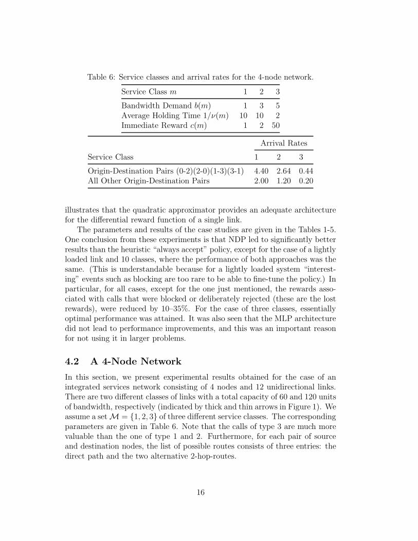
Table 6: Service classes and arrival rates for the 4-node network.

Service Class m 1 2 3

Bandwidth Demand b(m) 1 3 5Average Holding Time 1/ν(m) 10 10 2Immediate Reward c(m) 1 2 50

Arrival Rates

Service Class 1 2 3

Origin-Destination Pairs (0-2)(2-0)(1-3)(3-1) 4.40 2.64 0.44All Other Origin-Destination Pairs 2.00 1.20 0.20

illustrates that the quadratic approximator provides an adequate architecturefor the differential reward function of a single link.

The parameters and results of the case studies are given in the Tables 1-5.One conclusion from these experiments is that NDP led to significantly betterresults than the heuristic “always accept” policy, except for the case of a lightlyloaded link and 10 classes, where the performance of both approaches was thesame. (This is understandable because for a lightly loaded system “interest-ing” events such as blocking are too rare to be able to fine-tune the policy.) Inparticular, for all cases, except for the one just mentioned, the rewards asso-ciated with calls that were blocked or deliberately rejected (these are the lostrewards), were reduced by 10–35%. For the case of three classes, essentiallyoptimal performance was attained. It was also seen that the MLP architecturedid not lead to performance improvements, and this was an important reasonfor not using it in larger problems.

4.2 A 4-Node Network

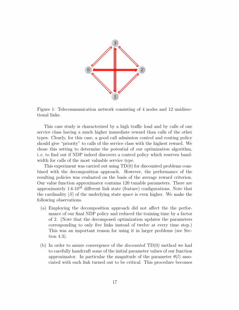
In this section, we present experimental results obtained for the case of anintegrated services network consisting of 4 nodes and 12 unidirectional links.There are two different classes of links with a total capacity of 60 and 120 unitsof bandwidth, respectively (indicated by thick and thin arrows in Figure 1). Weassume a set M = 1, 2, 3 of three different service classes. The correspondingparameters are given in Table 6. Note that the calls of type 3 are much morevaluable than the one of type 1 and 2. Furthermore, for each pair of sourceand destination nodes, the list of possible routes consists of three entries: thedirect path and the two alternative 2-hop-routes.

16

PSfrag replacements 0

1

2

3

4

Figure 1: Telecommunication network consisting of 4 nodes and 12 unidirec-tional links.

This case study is characterized by a high traffic load and by calls of oneservice class having a much higher immediate reward than calls of the othertypes. Clearly, for this case, a good call admission control and routing policyshould give “priority” to calls of the service class with the highest reward. Wechose this setting to determine the potential of our optimization algorithm,i. e. to find out if NDP indeed discovers a control policy which reserves band-width for calls of the most valuable service type.

This experiment was carried out using TD(0) for discounted problems com-bined with the decomposition approach. However, the performance of theresulting policies was evaluated on the basis of the average reward criterion.Our value function approximator contains 120 tunable parameters. There areapproximately 1.6·1045 different link state (feature) configurations. Note thatthe cardinality |S| of the underlying state space is even higher. We make thefollowing observations.

(a) Employing the decomposition approach did not affect the the perfor-mance of our final NDP policy and reduced the training time by a factorof 2. (Note that the decomposed optimization updates the parameterscorresponding to only five links instead of twelve at every time step.)This was an important reason for using it in larger problems (see Sec-tion 4.3).

(b) In order to assure convergence of the discounted TD(0) method we hadto carefully handcraft some of the initial parameter values of our functionapproximator. In particular the magnitude of the parameter θ(l) asso-ciated with each link turned out to be critical. This procedure becomes

17

PSfrag replacements

0 5 10

110

120

130

140

150

160

×106

Performance During Learning

steps

aver

age

rew

ard

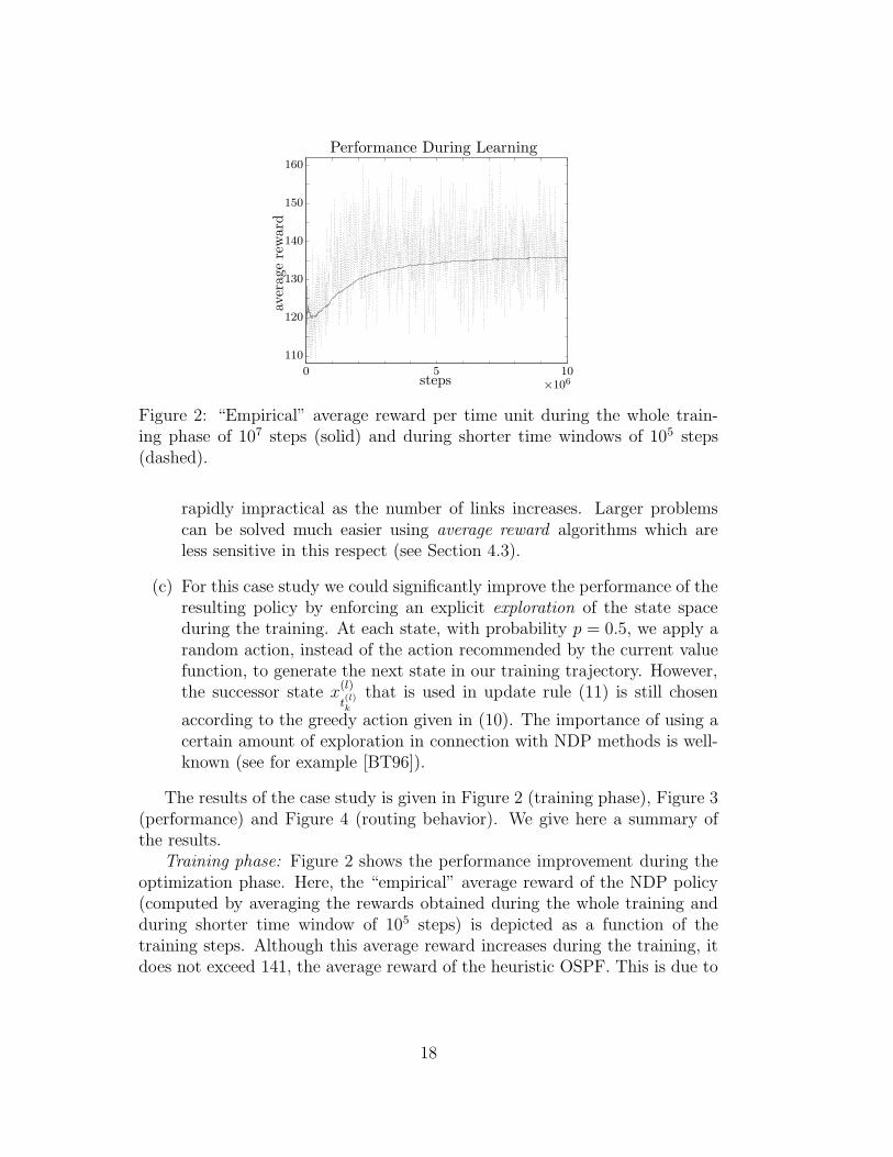
Figure 2: “Empirical” average reward per time unit during the whole train-ing phase of 107 steps (solid) and during shorter time windows of 105 steps(dashed).

rapidly impractical as the number of links increases. Larger problemscan be solved much easier using average reward algorithms which areless sensitive in this respect (see Section 4.3).

(c) For this case study we could significantly improve the performance of theresulting policy by enforcing an explicit exploration of the state spaceduring the training. At each state, with probability p = 0.5, we apply arandom action, instead of the action recommended by the current valuefunction, to generate the next state in our training trajectory. However,the successor state x

(l)

t(l)k

that is used in update rule (11) is still chosen

according to the greedy action given in (10). The importance of using acertain amount of exploration in connection with NDP methods is well-known (see for example [BT96]).

The results of the case study is given in Figure 2 (training phase), Figure 3(performance) and Figure 4 (routing behavior). We give here a summary ofthe results.

Training phase: Figure 2 shows the performance improvement during theoptimization phase. Here, the “empirical” average reward of the NDP policy(computed by averaging the rewards obtained during the whole training andduring shorter time window of 105 steps) is depicted as a function of thetraining steps. Although this average reward increases during the training, itdoes not exceed 141, the average reward of the heuristic OSPF. This is due to

18

PSfrag replacements

Average Reward

potential rewardreward obtained by NDPreward obtained by OSPF

reward per time unit

Comparison of Rejection Rates

OSPF policy

NDP policy

percentage of calls rejected

service type

0

50

100 150 200 250

1

2

3

0

5

10

15

20

25

30

35

40

45 50

PSfrag replacements

Average Reward

potential reward

reward obtained by NDP

reward obtained by OSPF



OSPF policyNDP policy


serv

ice

type

0

50

100

150

200

250

1

2

3

0 5 10 15 20 25 30 35 40 45 50

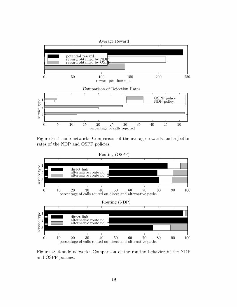
Figure 3: 4-node network: Comparison of the average rewards and rejectionrates of the NDP and OSPF policies.

PSfrag replacements

Average Reward

potential reward





OSPF policy

NDP policy


serv

ice

type

0

50

100

150

200

250

1

2

3

0

5

10

15

20

25

30

35

40

45

50

Routing (OSPF)

direct linkalternative route no. 1alternative route no. 2

percentage of calls routed on direct and alternative paths

Routing (NDP)

0 10 20 30 40 50 60 70 80 90 100

PSfrag replacements

Average Reward

potential reward





OSPF policy

NDP policy


serv

ice

type

0

50

100

150

200

250

1

2

3

0

5

10

15

20

25

30

35

40

45

50Routing (OSPF)

direct linkalternative route no. 1alternative route no. 2


Routing (NDP)

0 10 20 30 40 50 60 70 80 90 100

Figure 4: 4-node network: Comparison of the routing behavior of the NDPand OSPF policies.

19

the high amount of exploration in the training phase. We obtained the finalcontrol policy after 107 iteration steps.

Performance comparison: We used simulated trajectories of 107 time stepsto evaluate our policies. The policy obtained through NDP gives an averagereward of 212, which as about 50% higher than the one of 141 achieved byOSPF. Furthermore, the NDP policy reduces the number of rejected calls forall service classes. The most significant reduction is achieved for calls of serviceclass 3, the service class, which has the highest immediate reward. Figure 3also shows that the average reward of the NDP policy is close to the potentialaverage reward of 242, which is the average reward we would obtain if all callswere accepted. This leaves us to believe that the NDP policy is close to optimal.Figure 4 compares the routing behavior of the NDP control policy and OSPF.While OSPF routes about 15%-20% of all calls along one of the alternative2-hop-routes, the NDP policy uses alternate routes for calls of type 3 (about25%) and routes calls of the other two service classes almost exclusively overthe direct route. This indicates, that the NDP policy uses a routing scheme,which avoids 2-hop-routes for calls of service class 1 and 2, and which allowsus to use network resources more efficiently.

4.3 A 16-Node Network

In this section, we present experimental results obtained for a network con-sisting of 16 nodes and 62 unidirectional links (see Figure 5). The networktopology is taken from [GS97]. The network consists of three different classesof links with a capacity of 60, 120 and 180 units of bandwidth, respectively.We assume four different service classes. Table 7 summarizes the correspond-ing bandwidth demands, average holding times and immediate rewards. Thetable of arrival rates is also taken from [GS97]. However, for our experimentswe rescaled them by a factor of 2. The list of accessible routes consists of amaximum of six minimal hop routes for each pair of source and destinationnodes. Routes with an equal number of hops are ordered by their absolutepath length (in miles) which is also reported in [GS97].

For this experiment, there are approximately 1.4·10256 different link state(feature) configurations and 992 tunable parameters. The results of the casestudy are summarized by Figure 6 (training), Figure 7 (performance), Figure 8(routing), and Figure 9 (robustness).

We make the following observations.

(a) Without using the decomposition approach, no substantial improvementover the initial policy is achieved within a reasonable amount of com-

20

PSfrag replacements

0

1

2

3

4

5

6

7

8

9

10

11

12

13

14

15

Figure 5: Telecommunication network consisting of 16 nodes and 62 unidirec-tional links.

Table 7: Service classes for the 16-node network.

Service Class m 1 2 3 4

Bandwidth Demand b(m) 1.00 2.00 3.00 4.00Average Holding Time 1/ν(m) 1.25 1.25 1.25 1.25Immediate Reward c(m) 0.25 1.00 6.00 15.00

21

PSfrag replacements

0 2 4 6 8 10 12 14 16 183900

4000

4100

4200

4300

4400

4500

4600

×105steps

aver

age

rew

ard

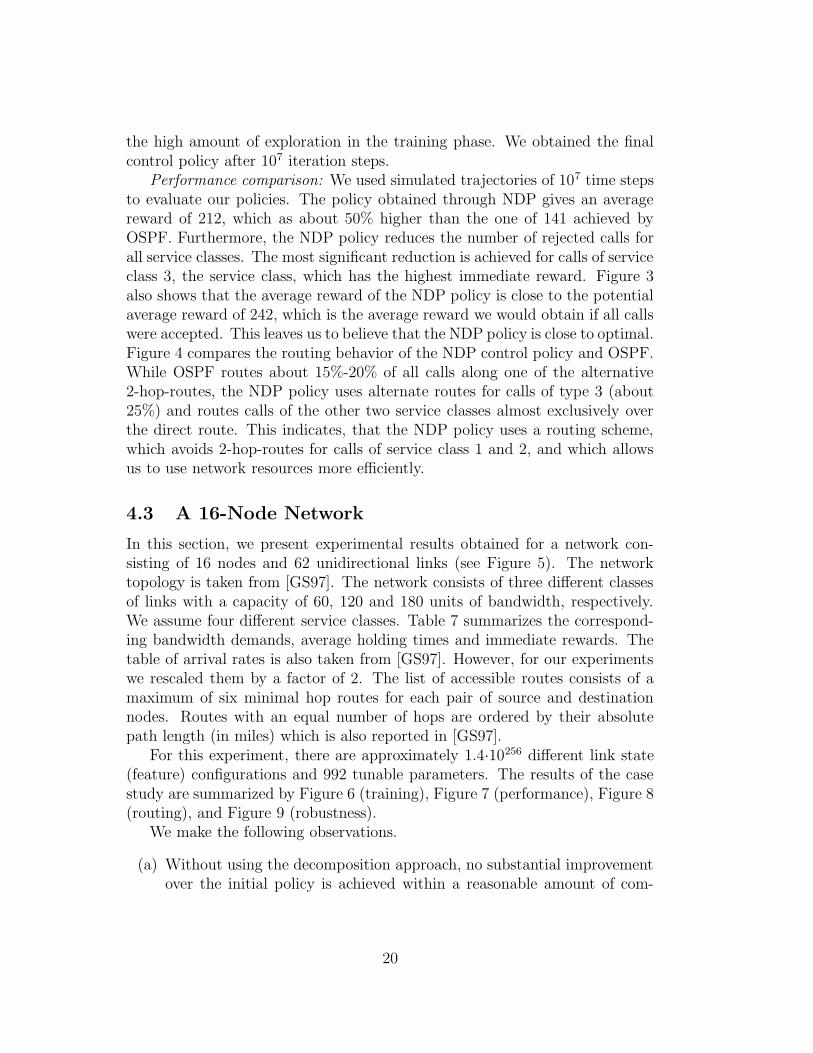
Figure 6: “Empirical” average reward obtained during the training as a func-tion of training steps. The performance initially improves and then suddenlydeteriorates.

putation time (24 hours, say). This illustrates the importance of thedecomposition approach in applying NDP to the call admission controland routing problem.

(b) Discounted reward algorithms failed due to their critical dependence oninitial parameter values (see Section 4.2). This difficulty does not arisewith average reward algorithms.

(c) Instabilities can occur during the training phase, even when explorationis employed (see the discussion below).

(d) Our NDP policies are very robust with respect to changes of the under-lying arrival statistics.

Training phase: Figure 6 shows the “empirical” average reward of theNDP policy (computed by averaging the rewards obtained during the simula-tion run) as a function of the training steps. In contrast to the 4-node examplethe NDP policy does not converge towards a final policy better than OSPF,although the average reward significantly improved during the first 4·105 train-ing steps. Afterwards, a sudden performance breakdown occurs, from whichthe system never recovers. This loss of stability did not disappear, even if weintroduce explicit exploration during the training. For the subsequent perfor-mance comparison between NDP and OSPF we pick the best policy (given by

22

the parameter values just before the loss of stability) generated in the courseof the algorithm, not the last one.

Performance comparison: The policies are empirically evaluated based onsimulated trajectories of 107 time steps. The OSPF policy almost exclusivelyroutes all calls over the shortest path. This leads to an average reward ofabout 4254. The rate of rejected calls is positive for all service classes. Thetwo most valuable service classes 3 and 4 receive the highest rejection rate.In contrast, the NDP policy comes up with a very different routing schemethat uses alternative paths for all types of services. Now, the rejection ratesfor calls of type 1, 3 and 4 vanish whereas that for service class 2 increases.The NDP policy rejects these calls in a strategic way, i. e. NDP is not forcedto do so by the capacity constraint. Instead, it explicitly reserves bandwidthfor the most valuable calls of type 3 and 4. The average reward of 4349 ob-tained through the NDP policy is about 2.2% higher than the one achieved byOSPF. While this might appear to be a small improvement, it has to be viewedin perspective: even if we could achieve the potential average reward (whichis 4438) by accepting every arriving call, the reward would only increase by4.3%. Thus, the 2.2% improvement in rewards, is a substantial fraction of thebest possible improvement. In fact, NDP reduces the lost average reward (po-tential average reward minus actual average reward) by about 52% comparedwith OSPF. Note that for this type of problems, the lost average reward is amore meaningful performance measure than the average reward. For example,if we have a single link and a single service class, it coincides with the blockingprobability (rejection rate), which is the generally accepted performance met-ric. Blocking probabilities in well-designed systems are generally small, andan improvement from, say, 4% to 2% is generally viewed as substantial, eventhough it only represents a 2% increase of calls accepted.

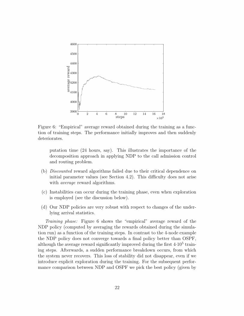
Robustness: We applied our best policy obtained through training underthe above mentioned arrival statistics to problems with randomly changed ar-rival rates in order to show the robustness of NDP policies. In particular, eacharrival rate is multiplied by a factor 1 + ρ, where ρ ∈ [−α, α] is independentlydrawn from a uniform distribution. An arrival rate is set to zero, if 1 + ρhappens to be negative. We carried out a set of experiments by varying themagnitude α ∈ [0, 2] in steps of 0.1, which amounts to rather strong perturba-tions of the traffic statistics. Figure 9 shows the result of these experiments.The magnitude α of the relative perturbations of the arrival rates is depictedagainst the relative lost reward defined as

v(µndp) − v(µospf)

vpotential − v(µospf).

23

PSfrag replacements

Average Reward

potential rewardreward obtained by NDPreward obtained by OSPF



OSPF policy

NDP policy


service type

3500 3600 3700 3800 3900 4000 4100 4200 4300 4400 4500

0

1

2

3

4

5

6

7

8

9

10

PSfrag replacements

Average Reward

potential reward





OSPF policyNDP policy


serv

ice

type

3500

3600

3700

3800

3900

4000

4100

4200

4300

4400

4500

0

1

1

2

2

3

3

4

4 5 6 7 8 9 10

Figure 7: 16-node network: Comparison of the average rewards and rejectionrates of the NDP and OSPF policies.

PSfrag replacements

Average Reward

potential reward





OSPF policy

NDP policy


serv

ice

type

3500

3600

3700

3800

3900

4000

4100

4200

4300

4400

4500

0

1

2

3

4

5

6

7

8

9

10

Routing (OSPF)

shortest pathalternative route no. 1alternative route no. 2alternative route no. 3alternative route no. 4alternative route no. 5


Routing (NDP)

0 10 20 30 40 50 60 70 80 90 100

PSfrag replacements

Average Reward

potential reward





OSPF policy

NDP policy


serv

ice

type

3500

3600

3700

3800

3900

4000

4100

4200

4300

4400

4500

0

1

2

3

4

5

6

7

8

9

10Routing (OSPF)

shortest pathalternative route no. 1alternative route no. 2alternative route no. 3alternative route no. 4alternative route no. 5


Routing (NDP)

0 10 20 30 40 50 60 70 80 90 100

Figure 8: 16-node network: Comparison of the routing behavior of the NDPand OSPF policies.

24

PSfrag replacements

rela

tive

lost

rew

ard

magnitude α of relative changes of the arrival rates

0

0

0.2

0.2

0.4

0.4

0.6

0.8 1.0 1.2 1.4 1.6 1.8 2-0.2

-0.1

0.1

0.3

0.5

0.6

0.6

0.7

Figure 9: Relative lost reward of the NDP policy applied to networks withrandomly changed arrival statistics.

Here, vpotential, µndp and µospf denote the potential average reward, the NDPpolicy and the OSPF policy, respectively. The experiments show, that ourNDP policy is indeed very robust against changes in the arrival rates. Thereis only one out of twenty experiments where the NDP policy happened tobe worse then OSPF. (We did not average several experiments with equalperturbation parameter α.) For all other arrival statistics the NDP policy stilloutperforms OSPF with a relative lost reward between 25% and 70%.

5 Conclusion

The call admission control and routing problem for integrated service net-works is naturally formulated as an average reward dynamic programmingproblem, but with a very large state space. Traditional dynamic programmingmethods are computationally infeasible for such large scale problems. We useneuro-dynamic programming, based on the average reward TD(0) method of[TV97b], combined with a decomposition approach that views the network asconsisting of decoupled link processes. This decomposition has the advantagethat it allows for decentralized decision making and decentralized training,which reduces significantly the training time. We have presented experimentalresults for several example problems, of different sizes. The case study in-volving a 16-node network shows that NDP can lead to sophisticated controlpolicies involving strategic call rejections, and which are difficult to obtain

25

through heuristics.Compared with the heuristic OSPF, the NDP policy reduces the lost av-

erage reward by 50% (heavily loaded 4 node network), 52% (lightly loaded16 node network), and (except for one out of twenty experiments) by 20-70%(16 node network under different loads). This illustrates that NDP has thepotential to significantly improve performance over a broad range of networkloads.

Concerning the practical applicability of this general methodology, thereare two somewhat distinct issues. The first is whether dynamic policies basedon state-dependent costs (depending linearly on the variables nl,m) can leadto significant performance improvements. Our results suggest that this is in-deed the case, although a comparison with alternative policies (such as dy-namic alternative routing with trunk reservation) remains to be made. Asomewhat related issue is whether efficient performance evaluation tools arepossible (based on ideas similar to the reduced load approximation, that donot involve simulation) which apply to policies of the form considered in thispaper.

The second issue refers to computational requirements. Simulation-basedmethods such as TD can be slow. For example, the computation times forour different experiments ranged from one to four hours of CPU time on aSun Sparc 20 workstation. On the other hand, once we can see promise in anapplication domain, a variety of ways of improving speed can be considered.Besides optimizing the code, these could include batch linear least squaresmethods for tuning θ (to replace small step size incremental training), or theuse of a smaller set of tunable parameters after identifying those “features”that are most critical for improved performance. Nevertheless, it seems thatNDP is best suited as a tool for off-line rather than on-line optimization of thecall admission control and routing policy.

It should be noted that while the (off-line) training time of the NDP policycan be in the order of minutes or hours, the “complexity” of implementing(on-line) a NDP policy (for a fixed parameter vector) is very similar to the oneof OSPF, i. e. the “cost” of a route can be determined by simply adding up thecorresponding “link shadow prices”, which are given by a quadratic functions.

References

[Ber95] D.P. Bertsekas, Dynamic Programming and Optimal Control. AthenaScientific, Belmont, MA, 1995.

26

[BT96] D.P. Bertsekas, and J.N. Tsitsiklis, Neuro-Dynamic Programming.Athena Scientific, Belmont, MA, 1996.

[BTS99] T.X. Brown, H. Tong, and S. Singh, “Optimizing admission controlwhile ensuring quality of service in multimedia networks via reinforcementlearning”. To appear in Advances in Neural Information Processing Sys-tems 11, MIT Press, Cambridge, MA, 1999.

[CN99] J. Carlstrom, and E. Nordstrom, “ Reinforcement learning for controlof self-similar call traffic in broadband networks”. Teletraffic Engineeringin a Competitive World, Proceedings of the 16th International TeletrafficCongress (ITC 16), P. Key, D. Smith (eds.), pp. 571–580, Elsevier, Edin-burgh, UK, 1999.

[CR93] S. Chung, and K.W. Ross, “Reduced load approximations for multi-rate, multi-hop communication networks”. IEEE Trans. Commun., vol. 41,no. 8, August 1993.

[DM94] Z. Dziong, and L.G. Mason, “Call admission and routing in multi-service loss networks”. IEEE Trans. Commun., vol. 42, no. 2/3/4, Febru-ary/March/April 1994.

[GS97] A. Greenberg, and R. Srikant, “Computational techniques for accurateperformance evaluation in multirate, multihop communication Networks”.IEEE/ACM Transactions on Networking, vol. 5, no. 2, April 1997.

[Hay94] S. Hayking, Neural Networks: A Comprehensive Foundation. McMil-lian, N.Y., 1994.

[Kel88] F. P. Kelly, “Routing in circuit switched networks: optimization, sha-dow prices and decentralization”. Adv. Appl. Prob., vol. 20, 1988.

[Kel91] F. P. Kelly, “Loss networks”. Annals of Applied Probability, vol. 1, pp.319–378, 1991.

[Key90] P.B. Key, “Optimal control and trunk reservation in loss networks”.Prob. Engrn. Inf. Sci.,vol. 4, pp. 203–242, 1990.

[Laws95] C.N. Laws, “On trunk reservation in loss networks”. In StochasticNetworks, F. P. Kelly and R. J. Williams (eds.), vol. 71 of IMA Volumesin Mathematics and its Applications, pp. 187–198. Springer-Verlag, NewYork, 1995.

27

[LBM98] M.Y. Liu, J. S. Baras, and A. Misra, “Performance evaluation inmulti-rate, multi-hop communication networks with adaptive routing”.ARL Federated Laboratory 2nd Annual Conference, University of Mary-land, College Park, MD, February 1998.

[Liu97] M.Y. Liu, Performance evaluation in multi-rate multi-hop communi-cation networks. Master’s thesis, U. Maryland, College Park, MD 1997.Available from http://www.isr.umd.edu/TechReports/ISR/1997.

[MT97] P. Marbach, and J.N. Tsitsiklis, A Neuro-Dynamic Programming Ap-proach to Call Admission Control in Integrated Service Networks: The Sin-gle Link Case. Technical Report LIDS-P-2402, Laboratory for Informationand Decision Systems, Massachusetts Institute of Technology, November1997. Available from http://web.mit.edu/jnt/www/publ.html.

[MMR96] D. Mitra, J.A. Morrison, and K.G. Ramakrishnan, “ATM networkdesign and optimization: a multirate loss network framework”. IEEE/ACMTransactions on Networking, vol. 4, no. 4, August 1996.

[NC95] E. Nordstrom, and J. Carlstrom, “A reinforcement learning schemefor adaptive link allocation in ATM networks”. Proceedings of the Interna-tional Workshop on Applications of Neural Networks to Telecommunication2 (IWANNT*95), J. Alspector, R. Goodman, T.X. Brown (eds.), pp. 88–95, Lawrence Erlbaum, Stockholm, Sweden, 1995.

[Ros95] K.W. Ross, Multiservice Loss Models for Broadband CommunicationNetworks. Springer-Verlag, Berlin, Heidelberg, New York, 1995.

[SiB97] S. Singh, and D.P. Bertsekas, “Reinforcement learning for dynamicchannel allocation in cellular telephone systems”. In M.C. Mozer andM. I. Jordan and T. Petsche (eds.), Advances in Neural Information Pro-cessing Systems 9, pp. 974–980. MIT Press, Cambridge, MA, 1997.

[Sut88] R. S. Sutton, “Learning to predict by the methods of temporal differ-ences”. Machine Learning, vol. 3, pp. 9–44, 1988.

[SB98] R. S. Sutton, and A.B. Barto, Reinforcement Learning: An Introduc-tion. MIT Press, Cambridge, MA, 1998.

[Tes88] J. Tesauro, “Practical issues in temporal difference learning”. MachineLearning, vol. 8, 1988.

28

[TV97a] J.N. Tsitsiklis, and B. Van Roy, “An Analysis of Temporal-DifferenceLearning with Function Approximation”. IEEE Transactions on AutomaticControl, vol. 42, no. 5, pp. 674–690, May 1997

[TV97b] J.N. Tsitsiklis, and B. Van Roy, Average cost temporal-differencelearning. Lab. for Info. and Decision Systems Report LIDS-P-2390, Mas-sachusetts Institute of Technology, Cambridge, MA; accepted for publica-tion in Automatica, 1997.

[WV96] J. Walrand, and P. Varaiya, High-Performance Communication Net-works. Morgan Kaufman, San Francisco, CA, 1996.

[Whi88] P. Whittle, “Approximation in large-scale circuit-switched networks”.Prob. Engrn. Inf. Sci.,vol. 2, pp. 279–291, 1988.

[ZD96] W. Zhang, and T.G. Dietterich, “High performance job-shop schedul-ing with a time-delay TD(λ) network”. In D. S. Touretzky, M.C. Mozer andM.E. Hasselmo (eds.), Advances in Neural Information Processing Systems8, pp. 1024–1030. MIT Press, Cambridge, MA, 1996.

29

call admission control and routing in integrated …honavar/rl-call.pdfsubmitted to ieee journal on...

Documents