Call Sequence Prediction through Probabilistic Calling Automata

Zhijia Zhao, Bo Wu⇧, Mingzhou Zhou, Yufei Ding†, Jianhua Sun, Xipeng Shen†, Youfeng Wu⇤

College of William and Mary ⇧ Colorado School of Mines † North Carolina State University ⇤Intel Labs{zzhao,mzhou,jianhua}@cs.wm.edu

⇧bwu@mines.edu

†{yding8,xshen5}@ncsu.edu ⇤youfeng.wu@intel.com

Abstract

Predicting a sequence of upcoming function calls is impor-tant for optimizing programs written in modern managedlanguages (e.g., Java, Javascript, C#.) Existing function callpredictions are mainly built on statistical patterns, suitablefor predicting a single call but not a sequence of calls. Thispaper presents a new way to enable call sequence predic-tion, which exploits program structures through ProbabilisticCalling Automata (PCA), a new program representation thatcaptures both the inherent ensuing relations among func-tion calls, and the probabilistic nature of execution paths. Itshows that PCA-based prediction outperforms existing pre-dictions, yielding substantial speedup when being applied toguide Just-In-Time compilation. By enabling accurate, effi-cient call sequence prediction for the first time, PCA-basedpredictors open up many new opportunities for dynamic pro-gram optimizations.

Categories and Subject Descriptors D3.4 [ProgrammingLanguages]: Processors

General Terms Languages, Performance

Keywords Function call, Call sequence prediction, Prob-abilistic calling automata, Dynamic optimizations, Just-in-time compilation, Parallel compilation

1. Introduction

Languages with a managed environment—such as JAVA,Javascript, C#—become increasingly popular. Programs inthese languages often have a large number of functions, andfeature many dynamic properties. For them, knowing the up-coming sequence of function calls in a run can be helpful.For example, a feature in these languages is dynamic func-tion loading: Some classes or functions are loaded from local

Permission to make digital or hard copies of all or part of this work for personal orclassroom use is granted without fee provided that copies are not made or distributedfor profit or commercial advantage and that copies bear this notice and the full citationon the first page. Copyrights for components of this work owned by others than theauthor(s) must be honored. Abstracting with credit is permitted. To copy otherwise, orrepublish, to post on servers or to redistribute to lists, requires prior specific permissionand/or a fee. Request permissions from Permissions@acm.org.OOPSLA ’14, October 19 - 21 2014, Portland, OR, USACopyright is held by the owner/author(s). Publication rights licensed to ACM.ACM 978-1-4503-2585-1/14/10$15.00.http://dx.doi.org/10.1145/2660193.2660221

disks or remote servers during an execution [25]. The load-ing takes time. With the upcoming call sequence known, thedelay can be largely hidden through prefetching. As anotherexample, the runtime system supporting those languages, es-pecially on embedded systems, often uses a small chunkof memory (called code cache) to store the generated na-tive code for reuse. Knowing the upcoming call sequencecan enhance the code cache usage substantially [16]. It canalso help the runtime system decide when to invoke JITto compile which function and at which optimization lev-els [15], and so on. The benefits may go beyond the runtimeof managed languages. Co-design virtual machines [18], forinstance, use runtime Binary Code Translation to reconciledisparity between conventional ISA and native ISA. Its run-time translation also uses JIT, sharing similar opportunities.

Call sequence prediction is to provide such knowledgethrough prediction. It is challenging for the large scope ofprediction. The state of the art is yet preliminary. Most ofthem have concentrated on exploiting statistical patterns incall history [4, 23, 27], and predicting the next one callrather than a sequence of calls. This limited prediction scopedoes not well suit the many needs of runtime systems. Evenworse, as the scope enlarges, the regularity diminishes, form-ing a main barrier for existing prediction techniques.

In this paper, we present a new way to enable call se-quence prediction. It centers on an effective exploitation ofprogram structures. The rationale is that program structuresinherently define some constraints on function calling rela-tions, which often cast some deciding effects on function callsequences. Conceptually, the key of this approach is in de-veloping an expressive model of the relations among func-tion calls to effectively capture those constraints. To facili-tate runtime call sequence prediction, the model must distin-guish call sites, capture calling contexts, incorporate the in-fluence of branches and loops, and finally accommodate thevarious complexities in programs and language implemen-tations (e.g., function dynamic dispatch, function inlining,code coverage variations across inputs). Existing models—such as call graphs, call trees, and calling context trees [3]—meet some but not all these requirements.

We present Probabilistic Calling Automata (PCA), a newprogram representation that uses extended Deterministic Fi-nite Automata (DFA) to capture both the inherent ensuing

relations among functions, and the probabilistic nature ofexecution paths caused by branches, loops, and dynamic dis-patch. A PCA is composed of a number of augmented statemachines, with each encoding the control flows related func-tion calls in a function. The PCA features a return stack anda shadow stack for efficiently maintain calling contexts, an↵-stack to handle complexities brought by exceptions andunknown function calls, and the concept of v-nodes andcandidate tables for addressing calling ambiguities causedby polymorphism, function pointers, and dynamic dispatch.Serving as a unified representation for function calls, PCAincorporates static program structures with profiling infor-mation, supports easy runtime state tracking, and toleratesvarious complexities in practical deployment.

After presenting the definition, properties, constructionand usage of PCA in Section 2 and Section 3, we discuss theinsufficiencies of existing program representations in Sec-tion 4, introduce some metrics for call sequence predictionin Section 5, and then describe an empirical comparisonbetween PCA-based predictors and the extensions of threealternative methods, respectively based on Calling ContextTrees and statistical patterns. Experiments show that PCA-based predictor achieves 89% on average in a basic accu-racy metric, 20–50% higher than that of the other predic-tors. Through parallel JIT compilation, we demonstrate thata simple usage of the PCA-based prediction can lead to per-formance improvement by up to 32% (15% on average).

Overall, this work makes the following contributions:

• It introduces PCA, a novel representation of functionensuing relations in a program that captures the influencecast by control flows and calling contexts.

• It shows how PCA can be used to enable effective callsequence prediction with design choices and usage study,as well as a systematic comparison with alternatives.

• It provides a set of metrics for measuring the quality of acall sequence prediction at various levels. They may meetthe needs of different uses of the prediction.

• Finally, this work, for the first time, demonstrates the fea-sibility and benefit of accurate call sequence prediction,which opens up new opportunities for dynamic optimiza-tions in various layers of the execution stack.

2. Problem Definition and Design

Considerations

As the problem has not been systematically explored before,we first provide a formal definition as follows.

2.1 Definition of Call Sequence Prediction

Definition 1. A function call sequence of a program is asequence of the IDs of the functions in the order of theirinvocations in an execution time window.

Definition 2. Call Sequence Prediction: For a given exe-cution of program P , function call sequence prediction at a

time point t is to predict the function call sequence of P inthe time window that immediately follows t.

The time window is called prediction window. Its lengthis usually in logical time (e.g., the number of function calls),and may be fixed or vary. Depending on the windows’length, the prediction may happen many times during anexecution of a program. For a multithreading execution, theprediction can be at the whole program level including allthreads, or at the level of one or several specific threads.

Function call sequences are largely dictated by programstructures. A primary goal of this work is to examine howto leverage program structures for call sequence prediction.Conceptually, the problem is to develop a representationthat is effective in capturing the relevant constraints on callsequences coded in a program.

2.2 Design Considerations

Ensuing Relations vs. Calling Relations There are somecommonly used inter-procedural program representations,such as call graphs, call trees and calling context trees. Theyprimarily represent calling relations among functions. But acall sequence is about which call follows which—and hencean embodiment of a series of ensuing relations.

It is important to note the differences between these twokinds of relations. Calling relations are about what func-tions would be called by what functions, while ensuing re-lations are about what function would be called right af-

ter what function calls. Calling relations affect ensuing re-lations. Knowing Y as one of the callees of X, for instance,suggests that Y will be, with some uncertainty in the pres-ence of branches, called after a call to X. But when that callwill happen is not coded in the calling relation: It could beimmediate, several or hundreds of calls later. An example isthe call of “D()” by “A()” in the PCAExample code in Fig-ure 1 (a). For the loop before “D”, there could be zero orthousands of “C” being called before “D” is called. Con-versely, two adjacent function calls in a call sequence, say“V W”, does not entail that W must be called by V: Thatcall to W could be made by V, its caller, or any of its callingancestors— respectively illustrated by ”A C” in lines 10 and12, ”C D” in lines 12 and 14, and ”D B” in lines 14 and 6 inthe PCAExample.

Four Basic Properties to Consider So the first considera-tion in our design of program representation is that it mustcapture ensuing relations of function calls. Ensuing relationsnaturally relate with program control flows (e.g., branches,loops), and often differ from one call site to another and fromone calling context to another. So the representation shouldalso consider these factors. In addition, to be used in run-time call sequence prediction, the representation should bereasonable in size, resilient to program complexities, and ap-plicable to most executions of a program. We put these con-siderations together as follows, and call them the four basicproperties:

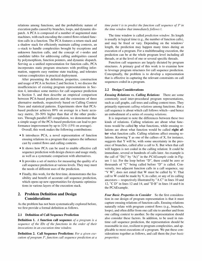
1: M( ){2: C( );3: if (...) A(1);4: else { 5: A(0);6: B( );}7: C( );8: A(2);9: }

10: A(x){11: for (){12: C( );13: }14: D( );15: }

(a) “PCAExample” program

M

C, 1 A,3 C, 5B, 4

A C,7.25

D,8

return stack

.75

shadow stack

A, 2

A, 6

.7

.3

I II

III

V

IV VVI

VII

VII

VIII

stack

(b) PCA

return

return

Figure 1. An example program named “PCAExample” and its PCA.

1 2 3 4A A DB

Figure 2. A DFA for code “A(); B(); A(); D();”.

• Ensuing relations: capturing ensuing relations amongfunction calls;

• Discriminating: discerning different control flows, callsites, and calling contexts1;

• Generality: being resilient to program complexities, suchas ambiguous calling targets in the presence of virtualfunctions, function dynamic dispatch, and so on;

• Scalability: having a bounded and acceptable size, re-gardless of the program execution length.

Existing representations were designed mainly for pro-gram analysis rather than call sequence prediction. Theycenter around calling relations, and fall short in some of thefour basic properties (detailed in Section 4). Because of theirinsufficiency, we propose the following design of PCA.

3. Probabilistic Calling Automaton (PCA)

Intuition PCA is in an augmented form of finite state au-tomata. Before defining it formally (in Section 3.6), we firstoffer some intuitive explanations. We choose automata as thebasic form for their natural fit for expressing ensuing rela-tions. For instance, Figure 2 shows an automaton for code“A( ); B( ); A( ); D( );”. The four nodes represent four stagesof an execution of the code. The DFA can easily track theexecution through state transitions: Upon the first call of thefunction “A”, it moves to state 1, and then to state 2 after“B” is invoked, and so on. The structure of the DFA reflectsthe ensuing relations of function calls imposed by the con-trol flow in the function—in Figure 2, a constraint is that “AD” but not any other sequences immediately follows the callof “B”. With this DFA, call sequence prediction becomes asimple walk over the DFA. For instance, suppose the DFA isnow at node 1. To predict the remaining call sequence, wecan simply walk along the DFA from node 1 and output thefunctions on the edges we bypass (“B A D” in this example.)

1 Here, calling context refers to the sequence of functions on the current callstack. A more precise context also includes parameter values, which furthercomplicates the problem. It is out of the scope of this work.

This example is simple, but conveys the basic idea ofPCA: Incorporating constraints defined by program codeinto a finite automaton and converting call sequence predic-tion into a walk over the automaton. For the idea to work,there are many challenges, some from program structures(e.g., branches, loops), some from language implementa-tions (e.g., function dynamic dispatching), some from com-piler transformations (e.g., function inlining and outlining).PCA addresses these challenges through a careful design.

To make the explanation easy to follow, we first draw onan example (PCAExample) rather than formalism to explainour PCA design and how it addresses various complexitiesfor runtime call sequence prediction. After that, we provide aformal, rigorous definition of PCA, along with the algorithmto construct it automatically.

3.1 Structure of PCA

A PCA consists of a number of finite state automata, andthree types of stacks. There is one automaton for each non-leaf function in the program. (A function is a leaf function ifits code contains no function calls; it is non-leaf otherwise.)

Nodes Each node in a PCA automaton corresponds to onecall site in the function. If the invoked function is non-leaf,we call the node a diamond, otherwise, a circle. Each nodecarries a label, written as hFunctionID, CallSiteIDi, where“FunctionID” and “CallSiteID” are the ID of the functioninvoked at that call site and the ID of the call site itself. (Aunique ID is assigned to every function and every call site.)A diamond carries an extra field, recording the address of theentry point of the automaton of the function called at the callsite represented by the diamond. This field allows smoothtransitions among automata of different functions.

When the “FunctionID” at a call site is either non-uniqueor unknown at the PCA construction time, “*” is used forthat field of the node. Such a node is called a v-node (vstands for virtual function). A v-node can be either a dia-mond or circle. The abstraction of v-nodes is important fortreating ambiguous function calls as Section 3.4 will show.

An automaton has a single entry node, and a single termi-nal node. They correspond to no call site, just indicating theentry and exit points of the automaton respectively.

Edges Edges in a PCA represent the ensuing relationsamong the function call sites contained in a function. There

is a directed edge from node A to node B in an automaton ifafter A’s call site (i.e., the call site represented by node A) isreached in an execution, node B’s call site could be reachedbefore any other call site in that automaton is reached. Notethat some call sites in other automata could be reached be-tween them. An example is the call of “A” on line 5 and thecall of “B” on line 6 in Figure 1 (a). The latter immediatelyfollows the former and hence there should be an edge be-tween their nodes, despite that the callees of function “A”are reached between the calls to “A” and “B”.

Each edge carries a label and a weight. The label is the IDof the sink node’s call site. It gives conveniences to trackingprogram state transitions in a call site discriminative manneras we will see later. The weight is the probability for thesink to follow the source in the program’s executions. Anedge flowing into a terminal node can have only “return” or“exit” as the label, indicating the exit of the function.

Stacks There are three stacks, associated with the entirePCA of a program. They are the return stack, shadow stack,and ↵-stack. The first two are designed to provide discrimi-nation of calling contexts, explained in Section 3.2. The thirdhelps handle unexpected function calls for practical deploy-ment of PCA, explained in Section 3.4.

Example Figure 1 (b) shows the PCA of the PCAExamplecode in Figure 1 (a). The top part shows the automaton offunction “M”. It contains three diamonds, all representingcalls of the non-leaf function “A” at the bottom. The threedotted lines are not PCA edges, but illustrations of the threediamonds’ references to the entry of A’s automaton. Entryand terminal nodes are shown as disks. Each node has itsID labeled. For instance, the diamond on top has a label“A,2”, meaning that this call site ID is “2” and the call is tofunction “A”. The edge from node “C,1” to “A,2” has label IIas it is the ID number of the call site represented by the sinknode. Its weight “.7” indicates that 70% instances of the callsite 1 are immediately followed by a call made at call site2 in function “M”. Weights equaling 1 are not shown forreadability. Theoretically speaking, the call site ID needs tobe labeled only on either the edge or in the sink node. Havingthe label at both places is for conveniences.

3.2 Basic Usage for Tracking and Prediction

The design of PCA makes it handy for efficient tracking thestate of a program execution and predicting its upcomingfunction calls.

Tracking Execution State To track the execution state of aprogram through PCA, we just need to let PCA transit to itsnext state upon every function call in an execution. An exit orreturn prompts a transit to its terminal state. When reaching adiamond node, the transition immediately moves to the entrynode of the corresponding automaton. For instance, a callat line 3 of PCAExample makes the PCA move from state“C,1” to “A,2”, and then immediately to the entry node ofthe automaton of function “A”. State transitions when a PCA

. . . . . .

execution starts

return stack

shadow stack

currentPCAstate

M

predictedcall seq.

after the first call to A A A,2

after a call to C C,7 A,2

call seq. pred. starts C,7 A,2 A,2

copy

pred. walk reaches node D,II A,2 A,2 C C C D

pred. walk reaches node A A A,2 C C C D C A

pred. walk reaches node D,II A,6 A,2 C C C D C A C C C C D

A,6

the pred. walk finishes A,6 A,2 C C C D C A C C C C D

execution resumes . . . . . .

exec

utio

nex

ec.

pred

ictio

n

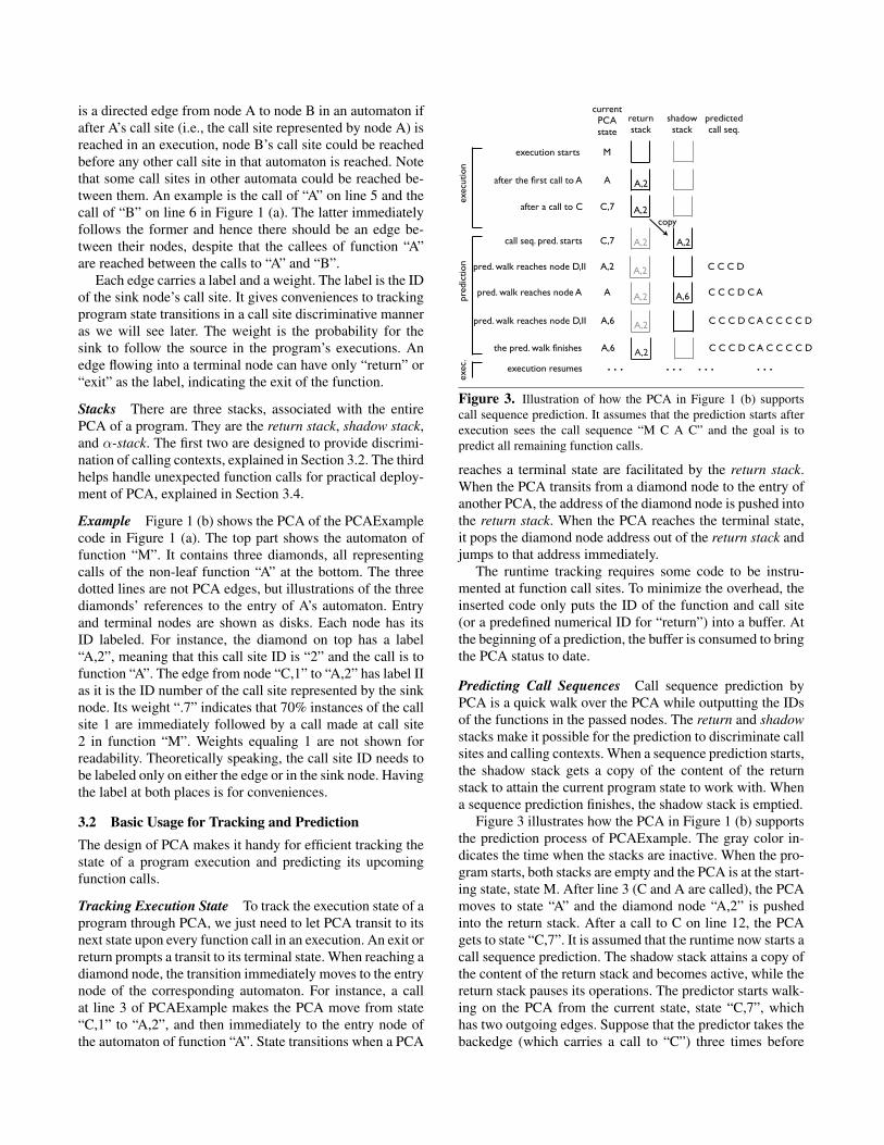
Figure 3. Illustration of how the PCA in Figure 1 (b) supportscall sequence prediction. It assumes that the prediction starts afterexecution sees the call sequence “M C A C” and the goal is topredict all remaining function calls.

reaches a terminal state are facilitated by the return stack.When the PCA transits from a diamond node to the entry ofanother PCA, the address of the diamond node is pushed intothe return stack. When the PCA reaches the terminal state,it pops the diamond node address out of the return stack andjumps to that address immediately.

The runtime tracking requires some code to be instru-mented at function call sites. To minimize the overhead, theinserted code only puts the ID of the function and call site(or a predefined numerical ID for “return”) into a buffer. Atthe beginning of a prediction, the buffer is consumed to bringthe PCA status to date.

Predicting Call Sequences Call sequence prediction byPCA is a quick walk over the PCA while outputting the IDsof the functions in the passed nodes. The return and shadowstacks make it possible for the prediction to discriminate callsites and calling contexts. When a sequence prediction starts,the shadow stack gets a copy of the content of the returnstack to attain the current program state to work with. Whena sequence prediction finishes, the shadow stack is emptied.

Figure 3 illustrates how the PCA in Figure 1 (b) supportsthe prediction process of PCAExample. The gray color in-dicates the time when the stacks are inactive. When the pro-gram starts, both stacks are empty and the PCA is at the start-ing state, state M. After line 3 (C and A are called), the PCAmoves to state “A” and the diamond node “A,2” is pushedinto the return stack. After a call to C on line 12, the PCAgets to state “C,7”. It is assumed that the runtime now starts acall sequence prediction. The shadow stack attains a copy ofthe content of the return stack and becomes active, while thereturn stack pauses its operations. The predictor starts walk-ing on the PCA from the current state, state “C,7”, whichhas two outgoing edges. Suppose that the predictor takes thebackedge (which carries a call to “C”) three times before

taking the edge (carrying a call to “D”) towards node “D,8”.That walk yields the predicted sequence “C C C D”. As node“D,8” leads to a terminal node, the shadow stack pops outnode “A,2” and the prediction walk immediately jumps tothat node. It is assumed that the walk then takes the edge tonode “C,5” and then to node “A,6” and outputs “C A” as theprediction. It then gets to node “A” again and continues theprediction. When the prediction finishes, the shadow stack isemptied and the return stack becomes active again.

The example touches one type of ambiguity in PCA: Anode has more than one outgoing edge, as exemplified bynodes “C,1” and “C,7”. We call this edge ambiguity. Edgeweights provide probabilistic clues on resolving the ambi-guity. We experiment with two policies for exploiting thehints. The first is the maximum likelihood (ML) approach,which always selects the edge with the largest weight. Thesecond is random walk, which chooses an edge with a prob-ability equaling the weight of that edge. For a node with k

outgoing edges, the approach works like throwing a k-sidedbiased dice, the biases of which equal the edge weights.

The ML approach seems to be subject to loops: Abackedge with a high probability may trap the predictor intothe loop2. However, when using PCA for call sequence pre-diction, the runtime queries the PCA occasionally. Hence,even though PCA might predict a seemingly-infinite loop,continued execution of the real program generally results inescaping the loop. A subsequent PCA query would then askabout execution following the loop. In practice, it outper-forms random walk in most cases as Section 6 will show.

3.3 Challenges for Practical Deployment

The aforementioned basic usage of PCA for prediction hastwo implicit assumptions:

1. Known-ID condition: The PCA construction can com-pletely determine the ID of the function to be invokedat every call site.

2. Completeness condition: The PCA captures all possibleand correct ensuing relations among function calls of aprogram.

The two conditions ensure that all call sequences occur-ring in an execution would be expected (and hence process-able) by the PCA. However, in many practical cases, the twoconditions do not hold due to the complexities in languageimplementation, compiler optimizations, and PCA construc-tion process. We will base our discussion mainly on a man-aged programming language (e.g., Java). Other types of lan-guages (e.g., C/C++) share some of those complexities.

Function Dynamic Dispatch The known-ID conditiondoes not always hold in the presence of function dynamicdispatch, with which feature, what function is called at acall site may remain unknown until the call actually hap-

2 If the edge weights get appropriately updated across iterations, ML maynot face such a problem.

/* a is an array of Animal that has a virtual function “voice()”; classAnimal has subclasses Cat, Dog, and Sheep.*/

1: for (i=0;i<N;i++){2: F();3: a[i].voice();4: G();5: }

Figure 4. An example of dynamic dispatch for polymorphism

pens. It often relates with polymorphism. For instance, sup-pose Cat, Dog, and Sheep are all subclasses of Animal, andthey all have their own implementation of the virtual func-tion “voice()” in Animal. The call to “a[i].voice()” at line3 in Figure 4 may actually invoke the “voice()” function ofany of the three classes, depending on which subclass a[i]is. Another common cause of dynamic dispatch is functionpointers, whose values may not be precisely determined atcompile time in a C program. No matter what the implemen-tation is, a common property of dynamic dispatch is that theexact function to be invoked at a call site sometimes cannotbe determined until the call happens. As an analogy to theedge ambiguity mentioned earlier, this issue can be regardedas node ambiguity. It is embodied by v-nodes in a PCA, thelabels of which have “*” as the FunctionID.

Compilation Complexities As Section 3.6 will show, PCAconstruction usually happens through some training runswith the help of compilers. In a managed environment, thecompilation is through a JIT compiler, and typically happensin every run. The compilation may differ in different runs,causing different ensuing relations among function calls,and hence the violation of the completeness condition. Forinstance, function inlining replaces a call site with the codeof the callee, while function outlining forms new functions inthe binary code. So different inlining and outlining decisionsin different runs could lead to different sets of call sites andensuing relations.

Furthermore, training runs and production runs may havea different coverage of the code. Some functions invokedin a production run may have never been encountered bythe JIT compiler in training runs, and hence may not appearin the constructed PCA. The training process could aggres-sively apply JIT to all possibly invoked functions, no matterwhether they are invoked in the training runs. However, dueto ambiguity in calling targets, it could end up including toomany irrelevant functions (e.g., an entire library excludinglibrary calls to JNI, which are not JITed).

Exception Handling Exception handling causes violationsto both conditions. In Java, it is usually implemented withstatic exception tables, which, similar to function pointers,cause fuzziness in function calling targets. At the same time,some exceptions (e.g., division by zero) are not checked.Similar to signal handlers in C code, there may be no explicitcalls to those handlers in the code, forming violations to thecompleteness condition.

Moreover, sometimes users may not be concerned of allfunctions. They, for instance, may not be interested in theinvocations of functions in the Java Runtime but only thosein the application. The bottom line is that some kind ofresilience to the incompleteness of PCA and node ambiguitywould be necessary for a practical deployment of PCA.

3.4 Solutions through v-Node and ↵-Stack

Features of v-nodes help address the issues related to theknown-ID condition. Each v-node is equipped with a candi-dates table. Every entry in the table indicates the possibilityfor that call site to be an invocation of a particular function.A threshold K is used to control the size of the table. Onlythe top K most likely candidates appear in the table. Fig-ure 5 shows the PCA for a variant of the “M” function in ourPCAExample, in which, the call to “A” at line 3 is replacedwith a function pointer whose most likely calling targets arefunctions “A” and “B”. Besides them, there is another 15%chance for the target to be some other functions. The proba-bilities of candidate targets are obtained through offline pro-filing, but adjustable at runtime as explained later.

During sequence prediction, the candidate table is usedfor speculating on the ID of the function to be invoked at thecorresponding call site. The speculation employs the samemethods as in resolving edge ambiguity (i.e., the ML orrandom walk method). The speculation happens every timewhen the prediction-oriented PCA walk reaches an v-node.

The issues on completeness condition are addressedthrough a combination of dynamic PCA evolvement and↵-stack. The dynamic evolvement is done at JIT time. Ourexamination shows that function inlining and outlining arethe major reasons for violations of the completeness condi-tion. The dynamic adjustment for inlining and outlining isstraightforward. Upon a function inlining, the JIT replacesthe node of that call site with the automaton of the inlinedfunction; upon a function outlining, the JIT creates an au-tomaton for the newly formed PCA, assigns an ID to thenew call site, and updates the automaton of the parent PCAaccordingly. As outlining happens rarely, negligible over-head was seen on the runtime PCA construction. The edgeweights of the newly created PCA are initiated with somevalues determined by the compiler (e.g., a policy commonin compiler construction is to put 0.9 for backedges and 0.5for normal two-way branches [36]).

As an option, during runtime, edge weights can be re-fined with the runtime observations through weighted aver-age (i.e., new weight = old weight*r + new observations*(1-r), 0.5 > r > 0) with the decay rate r set by the user. Suchan adjustment can be applied to other existing edges as well.(Our experiments did not use this runtime refinement.)

The ↵-stack addresses the issue of incomplete PCA (i.e.some functions do not have automata built). Initially the ↵-stack is empty and inactive. At an invocation of a functionthat has no automata built, the ID of the function is pushedinto the ↵-stack, and the ↵-stack becomes active. While the↵-stack is active, the ID of an invoked function is automat-

ically pushed into the stack, regardless of whether the func-tion has PCA; the top of the stack pops out at each func-tion return. The PCA stalls while the ↵-stack is active. Itresumes state transitions as soon as the ↵-stack becomes in-active when it turns empty. For example, suppose that thePCA is now in state “C,1” of Figure 1 (b) and some unex-pected function “X” is then invoked. Assume that “X” calls“Y” and “Y” calls “A”. Neither “X” nor “Y” has automatonbuilt. The PCA would stay at node “C,1” until “X” returns.It then resumes state transition according to the PCA.

Essentially, the ↵-stack makes operations on PCA skipfunctions that do not have automata, as well as the functionsdirectly or indirectly invoked by them. Such a design offersa simple way to deal with unexpected calls. A more sophisti-cated design is to skip only functions that have no automata(e.g., “X” and “Y” but not “A” in our example). It is poten-tially doable, but adds much complexity: It has to deal withbroken chains of states. For instance, when “A” returns, it isunclear which state the PCA should return to.

Additional complexities include native function calls andtail call optimizations. Native code is ignored. Optimized tailcalls become jump instructions and hence are not tracked orpredicted.

3.5 Properties

We now examine how PCA embodies the four basic proper-ties listed in Section 2.

(1) Ensuing relations. PCA is centered on ensuing rela-tions. A transition edge represents what function call follows(rather than invokes) another call. For example, in Figure 1(b), “C,5”!“A,6” represents that after the finish of “C” online 7 in Figure 1 (a) (represented by node “C,5”), the nextfunction call must be a call to “A” at line 8 (represented bynode “A,6”), despite that “C” never calls “A” in the program.

(2) Discriminating. The structure of PCA encodes bothbranches and loops. Its edge weights facilitate the resolutionof ambiguities caused by control flows. With node and edgelabels carrying call site IDs, PCA naturally distinguishes dif-ferent call sites. The return stack and shadow stack add call-ing contexts to PCA. For example, suppose the PCA is nowat state “C,7” in Figure 1 (b). The two stacks help the predic-tion automatically tell whether the call of “A” was from node“A,2”, “A,3”, or “A,6” when the PCA walk returns fromnode “D,8”, and hence produce different prediction results.In addition, the PCA structure allows an even deeper levelof discrimination: Instead of defining an edge weight as aprobability given the source node, one could employ condi-tional probabilities as edge weights, with the top k levels ofthe shadow stack as the conditions. In this way, they couldfurther discriminate call sites and calling contexts. Such amodel may increase the size of the PCA; we leave it to fu-ture study.

(3) Generality. The design of v-node and ↵-stack, alongwith runtime PCA evolvement, make PCA resilient to vari-ous complexities in the language implementation, compila-tion, and other aspects.

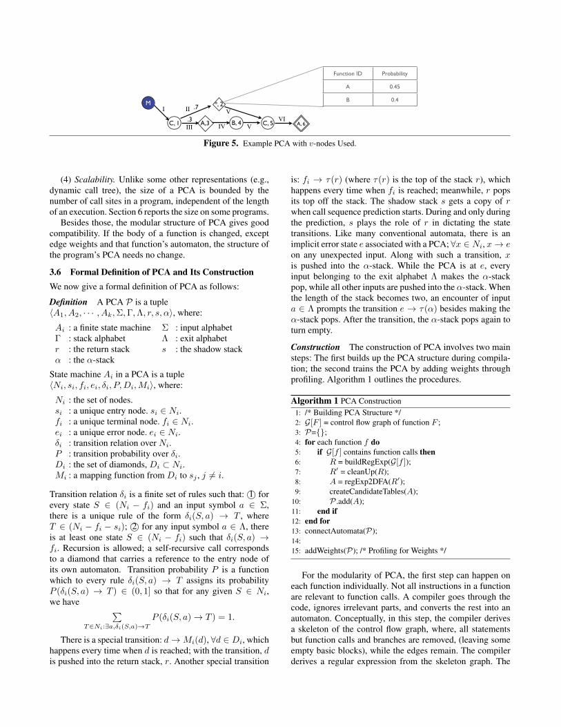
M

C, 1 A,3 C, 5B, 4

*, 2

A, 6

.7

.3

I II

III

V

IV VVI

Function ID Probability

A 0.45

B 0.4

Figure 5. Example PCA with v-nodes Used.

(4) Scalability. Unlike some other representations (e.g.,dynamic call tree), the size of a PCA is bounded by thenumber of call sites in a program, independent of the lengthof an execution. Section 6 reports the size on some programs.

Besides those, the modular structure of PCA gives goodcompatibility. If the body of a function is changed, exceptedge weights and that function’s automaton, the structure ofthe program’s PCA needs no change.

3.6 Formal Definition of PCA and Its Construction

We now give a formal definition of PCA as follows:

Definition A PCA P is a tuplehA1, A2, · · · , Ak,⌃,�,⇤, r, s,↵i, where:

Ai : a finite state machine ⌃ : input alphabet� : stack alphabet ⇤ : exit alphabetr : the return stack s : the shadow stack↵ : the ↵-stack

State machine Ai in a PCA is a tuplehNi, si, fi, ei, �i, P,Di,Mii, where:

Ni : the set of nodes.si : a unique entry node. si 2 Ni.fi : a unique terminal node. fi 2 Ni.ei : a unique error node. ei 2 Ni.�i : transition relation over Ni.P : transition probability over �i.Di : the set of diamonds, Di ⇢ Ni.Mi : a mapping function from Di to sj , j 6= i.

Transition relation �i is a finite set of rules such that: 1� forevery state S 2 (Ni � fi) and an input symbol a 2 ⌃,there is a unique rule of the form �i(S, a) ! T , whereT 2 (Ni � fi � si); 2� for any input symbol a 2 ⇤, thereis at least one state S 2 (Ni � fi) such that �i(S, a) !fi. Recursion is allowed; a self-recursive call correspondsto a diamond that carries a reference to the entry node ofits own automaton. Transition probability P is a functionwhich to every rule �i(S, a) ! T assigns its probabilityP (�i(S, a) ! T ) 2 (0, 1] so that for any given S 2 Ni,we have

PT2Ni:9a,�i(S,a)!T

P (�i(S, a) ! T ) = 1.

There is a special transition: d ! Mi(d), 8d 2 Di, whichhappens every time when d is reached; with the transition, dis pushed into the return stack, r. Another special transition

is: fi ! ⌧(r) (where ⌧(r) is the top of the stack r), whichhappens every time when fi is reached; meanwhile, r popsits top off the stack. The shadow stack s gets a copy of r

when call sequence prediction starts. During and only duringthe prediction, s plays the role of r in dictating the statetransitions. Like many conventional automata, there is animplicit error state e associated with a PCA; 8x 2 Ni, x ! e

on any unexpected input. Along with such a transition, xis pushed into the ↵-stack. While the PCA is at e, everyinput belonging to the exit alphabet ⇤ makes the ↵-stackpop, while all other inputs are pushed into the ↵-stack. Whenthe length of the stack becomes two, an encounter of inputa 2 ⇤ prompts the transition e ! ⌧(↵) besides making the↵-stack pops. After the transition, the ↵-stack pops again toturn empty.

Construction The construction of PCA involves two mainsteps: The first builds up the PCA structure during compila-tion; the second trains the PCA by adding weights throughprofiling. Algorithm 1 outlines the procedures.

Algorithm 1 PCA Construction1: /* Building PCA Structure */2: G[F ] = control flow graph of function F ;3: P={};4: for each function f do

5: if G[f ] contains function calls then

6: R = buildRegExp(G[f ]);7: R0 = cleanUp(R);8: A = regExp2DFA(R0);9: createCandidateTables(A);

10: P .add(A);11: end if

12: end for

13: connectAutomata(P);14:15: addWeights(P); /* Profiling for Weights */

For the modularity of PCA, the first step can happen oneach function individually. Not all instructions in a functionare relevant to function calls. A compiler goes through thecode, ignores irrelevant parts, and converts the rest into anautomaton. Conceptually, in this step, the compiler derivesa skeleton of the control flow graph, where, all statementsbut function calls and branches are removed, (leaving someempty basic blocks), while the edges remain. The compilerderives a regular expression from the skeleton graph. The

M ! m C1 (A2| (A3 B4)) C5 A6

A ! a C7+ D8

B ! bC ! cD ! d

Figure 6. The FCG of the program in Figure 1 (a). Every letterrepresents a function. An upper-case letter is a non-terminal vari-able, and a lower-case letter is a terminal variable, representing theprologue of a function represented with the corresponding upper-case letter, and a subscript represents a call site ID.

vocabulary of the regular expression consists of �, represent-ing an empty block in the skeleton graph, a terminal variableand a non-terminal variable for each function in the program.The � helps encode the logic of empty blocks into regu-lar expression. The non-terminal variable represents a callto the function. The terminal variable represents the entryof the function, which is always the first symbol in the regu-lar expression of the function. Branches are represented withthe “|” operator, while loops (or backedges) are representedwith the “*” or “+” operator.

Next, the compiler simplifies the regular expression ina standard way, which removes all �s as well. Figure 6shows the regular expressions of our PCAExample. We re-fer to such a set of regular expressions as the function call-ing grammar (FCG) of the program. As a whole, an FCGis a Context Free Grammar (CFG). The simple form di-rectly leads to PCA through standard algorithms of regularexpression-to-automaton conversion. Another advantage ofusing FCG as the intermediate form is that the conversionalgorithms, by default, minimize the generated automatonand hence the overall size of the PCA. The candidate tablesare then built for each v-node in the DFA.

The final step adds weights to the edges in the PCA. Ituses profiling executions of the program to do so. Duringa profiling run, the PCA runs along with it by updating itsstate upon each function call. A profiler records the numberof times an edge is visited if the out-degree of the source isgreater than one. The weight of an edge is then used to cal-culate the weights on those edges. It puts in the probabilitiesfor the entries in candidate tables in the same manner. Anedge that has not been encountered in the profiling runs isassigned with an extremely small weight for the complete-ness of the PCA.

What profiling mechanism to use is orthogonal to theproposal of PCA. Besides offline profiling, there are manyother techniques for efficient online sampling [9, 13, 20] orcross-run accumulation of samples [24]. They could all beused for PCA construction, depending on the usage scenario.

4. Comparisons to Existing Representations

Before this work, there are a variety of program represen-tations relevant to program function calls. In this section,we examine four most commonly studied ones, qualitativelyshowing that they are ill fit for call sequence prediction fornot meeting some of the four basic properties. Section 6

M

C A

D

B

M

C A

D

M

C A

D

C

C

M

C A

DC

C C C

(a) Static call graph (b) Dynamic call graph

(c) Dynamic call tree

(d) Calling context tree

A

DCC C C

Figure 7. Four other representations of function calls in execu-tions of “PCAExample” in Figure 1 (a). In the program, no func-tions except “M” and “A” contain function calls. In the consideredexecution, the “if” branch is taken.

will complement the comparison with some quantitative ev-idences.

Among existing models of program function calls, themost influential are static and dynamic call graphs, dynamiccall trees, and calling context trees (CCTs). We use Figure 7to review them briefly. In a static call graph (Figure 7 (a)),each function has a unique node no matter at how many callsites it is invoked, and there is an edge directed from func-tion “M” to function “A” if it is possible for “M” to call “A”.A dynamic call graph (Figure 7 (b)) has the same structure,except that it is built through a profiling run and there isan edge between two nodes only if that invocation actuallytakes place in that run. A dynamic call tree (Figure 7 (c)) alsocomes from a profiling run. It adds calling context informa-tion, with each node representing a function invocation, andthe path to it from the root representing its calling context. ACCT [3] is similar to a dynamic call tree except that it usesa single node to represent all calls to a function that have thesame calling contexts. In Figure 7 (d) for instance, all the“C” nodes under “A” in Figure 7 (c) are folded into one.

All four representations are designed for program anal-ysis rather than call sequence prediction. They have somevariations. We analyze their properties with their basic formsfirst, and discuss their extensions later. Specifically, we ex-amine them against the four basic properties, which qualita-tively reveals their limitations for call sequence prediction.

• Ensuing relations. The four representations are all cen-tered on calling relations rather than ensuing relations.For example, Figures 7 (a) (b) (c) and (d) all indicate thatboth “C” and “D” are possible callees of “A”, but noneencodes the relation that a call to “D” must follow calls

to “C” if those calls are made by “A”3. The lack of en-suing relations makes them fundamentally ill fit for callsequence prediction.

• Discriminating. Control flows: None of the four rep-resentations encodes branches or loops. The static callgraph in Figure 7 (a), for instance, fails to show that func-tion “A” is invoked at both branches and “B” is not. Theother three representations, on the other hand, completelymiss the branch that contains “B”. Moreover, none of therepresentations expresses that “C” is called inside a loop(the dynamic call tree in Figures 7 (c) shows four con-secutive calls to “C” in “A” but leaves it unclear whetherthey are caused by a loop or four different call sites of“C”.) Missing control flows hinders these representationsfor call sequence prediction. For example, the controlflows tell us that if and only if the second call sites of“A” is reached, “B” will be called immediately after “A”finishes. None of the four representations captures thatconstraint. Calling contexts: Dynamic call tree and CCTboth maintain calling contexts. But static and dynamiccall graphs do not. In Figures 7 (a) and (b), for instance,all calls to “C” are aggregated into a single node, despitethat they differ in their calling contexts. Call sites: Noneof the representations except dynamic call trees offers afull discrimination of call sites. For instance, the two sitesof calls to “C” in “M” are folded into a single node in Fig-ures 7 (a) (b) (d). They hence fail to encode that differentcall sequences could follow the two calls.

• Generality. Dynamic call graphs, call trees, and CCT allcontain only the invocations made in some training exe-cution(s) rather than the complete calling relations in theprogram. Some functions (e.g., “B”) absent from themmay be called in other runs. It is possible to append thesenewly encountered calls to these graphs or trees at run-time. But there are no machinery in these representationsto overcome the incompleteness and the ambiguity (e.g.,by dynamic dispatch) for call sequence prediction.

• Scalability. Static and dynamic call graphs are boundedby the number of unique functions in the program. CCTis bounded by the number of distinct calling contexts.They all have reasonable scalability, although sometimesa CCT could be orders of magnitude larger than theprogram itself. A dynamic call tree, on the other hand,may contain as many nodes as the number of functioninvocations in a run, often too large for practical usage.

Overall, in their basic forms, the four representations allmiss some of the basic properties. They have some varia-tions, the extra features of which may alleviate some issues,but cannot address their inherent limitations. For example,in a call graph with labeled edges, a caller may have mul-tiple calling edges connecting to a callee, with each edgecorresponding to a distinct call site. Similarly, CCT can be

3 Nodes in a dynamic call tree by default have no specific orders. If extendedwith a time order, the tree may capture some ensuing relations.

made call site-aware as well if different call sites of a func-tion are represented with different nodes, even if they havethe same calling context [32]. However, these variations donot change the inherent nature of these representations ofcentering around calling rather than ensuing relations. Nei-ther do they address the issues on control flows or generality.

Consequently, these representations cannot well capturethe relevant constraints defined by the program. In Figure 7,for example, none of them reflects the constraint that either“B” or “C” but not any other functions will follow the firstinvocation of “D”. Neither do they reflect that if “A” hasbeen invoked twice by “M” and the current execution pointis inside “D”, there will be definitely no other function callsby the end of the execution.

The qualitative analysis reveals the high-level limitationsof these representations for call sequence prediction; Sec-tion 6 confirms them through some quantitative comparisonswith PCA.

5. Metrics for Call Sequence Prediction

We find no prior definition of metrics for assessing a callsequence prediction. We introduce three levels of metrics,which are of different strictness, suitable for different usesof the prediction results.

Let Q and Q be the true and predicted call sequences, andU and U be the set of unique functions in Q and Q. The threelevels of metrics are as follows.

• Set-level: It quantifies the closeness between U and U .We introduce the following notations: TP = |U \ U |,TN = |U \ U |, FP = |U � U |, FN = |U � U |;U and U are the set of functions in the entire programthat do not appear in U or U respectively. (“T” for true,“F” for false, “N” for negative, “P” for positive.) Follow-ing information retrieval theory [17], we use two com-mon metrics: recall=TP/|U |; precision=TP/|U |. Theyrespectively measure how much the true set is uncoveredand how precise the prediction set is. To integrate theminto a single metric, we borrow the concept of Matthewscorrelation coefficient (MCC) [31], which takes into ac-count true and false positives and negatives and is gener-ally regarded as a balanced measure. It is defined asMCC= TP⇥TN�FP⇥FNp

(TP+FP )(TP+FN)(TN+FP )(TN+FN).

MCC has a value range [-1, 1]. We normalize it to [0, 1]as follows: Set accuracy=(MCC + 1)/2.

• Frequency-level: Let nf and nf be the numbers of timesthe function f appears in Q and Q respectively. Thefrequency accuracy of Q is1� averagef2U[U (|nf � nf |/max(nf , nf )).

• Sequence-level: Let e be the minimum number of atomicediting operations (insertion, deletion, or replacement ofa single token in Q) needed to change Q into Q. Thesequence accuracy of Q is 1�e/max(|Q|, |Q|). Let Q⇤

be the sequence of the functions in U ordered in their first

occurrences in Q, and Q

⇤ be the counterpart for Q. Thefirst-occ sequence accuracy is the sequence accuracy ofQ

⇤ regarding Q

⇤.

The usage of “max” in the frequency accuracy and se-quence accuracy ensures that the accuracy is in the range of 0and 100%. For instance, the e in sequence accuracy must beno greater than max(|Q|, |Q|) since a naive way to generateQ from Q is to replace every token in Q with the correspond-ing one in Q and its number of operations is max(|Q|, |Q|).

As an example, assume that the true sequence is “A AB C B D”, while the predicted sequence is “A A A B EF”, and there are 10 unique functions in the whole program.The measures are as follows: TP=2, TN=4, FP=2, FN=2, re-call=0.5, precision=0.5, set accuracy=0.58, frequency accu-racy=0.19, sequence accuracy=0.33, first-occ sequence ac-curacy=0.5.

Set-level measures are the most relaxed among all. Theyignore the order and frequency of function calls in the se-quences. First-occ sequence accuracy is slightly stronger byconsidering the order of the first-time occurrences of thefunctions in Q. They are useful when the prediction is forguiding early compilation or prefetching.

Frequency accuracy reflects how well the prediction cap-tures the hotness of the functions in Q. It is useful forhotness-based optimizations.

Sequence accuracy is the most strict on the differencebetween two sequences. The usage of atomic editing oper-ations in the definition avoids some misleading effects ofalternative definitions. For instance, Hamming distance—which does pair-wise comparison at token level—is sensi-tive to local differences and cannot precisely measure thesimilarity of two sequences. For example, Q is “A B C D”while Q is “E A B C”, accuracy based on Hamming dis-tance is 0, even though the two sequences share a large sub-sequence. The definition on atomic operations is not subjectto the problem. Computing the needed minimum number ofoperations can be challenging, but some existing tools (e.g.,the Linux utility “diff”) can be used as the ruler.

6. Evaluation

For evaluation, we concentrate on the following questions:

• Can PCA enable accurate call sequence predictions?What is the time and space cost?

• Is the enabled prediction useful?

For the first question, we design a set of experiments tomeasure the call sequence prediction accuracies and over-head; for the second question, we apply the prediction re-sults to help JIT decide when to compile which methods forreducing response time. It would be ideal to assess theseresults in the context of existing techniques. But it is diffi-cult as there are no existing work directly on call sequenceprediction. To circumvent the difficulty, we implement three

other call sequence predictors by extending most relevantexisting techniques.

6.1 Three Alternatives

In Machine Learning, there is a problem called discretesequence prediction [21], but its prediction target is still justthe next symbol in a sequence. To put our results into acontext, we implement two representatives of such methodsand extend them for call sequence prediction.

Alternative-1: The first is called Pattern method, an ex-tension from the single-call predictor by Lee and others [12,23]. It is based on Markov model. Through a Machine Learn-ing engine, it derives statistical patterns by examining all theK + 1-long subsequences of a training sequence, based onwhich, its predictor looks at the K most recent function callsto predict which function will be called next. The authorsshowed the usage of the prediction for detecting OS securityissues.

Alternative-2: The second is called TDAG method, whichalso exploits frequent subsequences but in a more sophisti-cated manner through a classical Machine Learning methodcalled Markov Tree [34]. It uses a tree to store frequentsubsequences of various lengths and maintains confidencefor each tree node. With the tree, it intelligently picks thebest subsequence (frequent enough with strong predictivecapability) for each prediction. To avoid tree size explo-sion, it adds some constraints on the nodes and height ofthe tree [21]. In our implementation, we adopt the same pa-rameter values as in the previous publication.

Both methods were originally designed for predictingonly the next symbol. We expand the prediction target nat-urally to a sequence of calls. The training process remainsthe same as in the previous work. At a prediction time, theextended methods gives prediction of the next symbol, ˆst+1,based on the previous k-symbol sequence (st�k+1, st�k+2,· · · , st) in their default manner, and then in the same manner,gives prediction ˆst+2 by regarding the sequence (st�k+2,st�k+3, · · · , ˆst+1) as the most recent k-symbol sequence.Other symbols in the time window are predicted likewise.A comparison to these methods helps reveal the benefits ofPCA’s capitalization of program inherent constraints.

Alternative-3: Although we are not aware of previous us-age of the other representations listed in Section 4 for callsequence prediction, they can be adapted to do so in a man-ner similar to our PCA. We implement such a predictor onCCT, the most sophisticated representation of all of them.It is called CCT-based predictor. There are two extensions.First, we add an edge from every node to each of its imme-diate parents (callers), representing the transition happeningwhen the current function returns. Second, we use profilingto add probabilities to all the edges in the extended CCT inthe same way as in PCA construction. As a program exe-cutes, each function call triggers one move on the CCT. Atprediction time, the predictor walks on the CCT based on thedirections of its edges, and outputs as the predicted sequencethe functions corresponding to the nodes it encounters. For a

node with multiple outgoing edges, we also experiment withboth the ML and random walk approaches.

A comparison to CCT-based predictor helps quantita-tively assess the benefits of PCA for its better treatment tocontrol flows, calling contexts and call sites.

6.2 Methodology

All experiments happen on a machine equipped with dual-socket quad-core Intel Xeon E5310 processors that runLinux 2.6.22; the heap size (”-Xmx”) is 512MB for all.We use Jikes RVM [1] (v3.1.2), an open-source Java Vir-tual Machine, as our basic framework. We modify its JIT toderive the FCG from a function’s bytecode, and to collectcalling sequence for training the edge weights on a PCA anda CCT. The Jikes RVM runs with the default JIT (includ-ing both baseline and optimizing compilation and inlining)unless noted otherwise.

We use the Dacapo (2006) benchmark suite [7]. ( Thelatest version of Dacapo does not work well with JikesRVM [19].) Two programs, chart and jython, were left outbecause they fail to run on the Jikes RVM-based profiler.Table 1 shows the benchmarks, their lines of code, the num-bers of unique calling contexts, and sequence lengths(i.e.,the total numbers of calls a program makes in a run) on thesmall and default inputs coming with the benchmark suite.In our experiment, we use small runs for training and defaultruns for testing. On most programs, the two runs differ sub-stantially in both the length of call sequences, as shown inTable 1, and the distribution of function calling frequenciesincluded in Appendix A. All executions involve a few JNIcalls. As Java uses dynamic dispatch, Table 2 reports thesize distribution of the candidate sets of function calls. Forall programs except for bloat, the call sites with larger than4 candidate set are less than 5%. We use ten as the upperbound of the candidate table size.

Our evaluation concentrates on the startup phase of pro-gram executions. Here, the startup phase refers to the be-ginning part of a program execution, by the end of which,a major portion of the methods that the whole executionneeds have been compiled. Quantitatively, we determine thestartup phase by finding the knee point on the cumulativecompilation curve of an execution. Figure 8 illustrates theconcept by depicting the curve of an execution of benchmarkbloat. Formally, a knee point on a smooth ascending convexcurve is defined as the point where the radius of curvatureis a local minimum. The cumulative compilation curve of aprogram execution are often not smooth, but its trend (i.e.,when local noises are smoothed out) is typically so. In ourexperiments, we draw all the cumulative compilation curvesof all executions and manually find the knee points throughvisual examination of the trend of the curves. We observethat the knee points of all of the program executions appearbefore the 700,000th function call in their executions. Forsimplicity, we take the first 700,000 function calls as the ap-proximated startup phases of all the programs in our evalua-

Table 1. Benchmark InformationProgram # code # unique call. Seq. length (⇥106)

lines contexts (⇥103) small defaultantlr 32263 1006 7 490bloat 73563 1980 9 6276eclipse 1903219 4816 18 1267fop 88846 175 3 44luindex 8570 374 10 740lusearch 12709 6 9 1439pmd 49331 8043 6 2727xalan 243516 163 33 10084

Table 2. Size of Candidate SetsProgram size distribution

1 2 3 4 �5antlr 73% 10% 9% 4% 4%bloat 49% 15% 8% 3% 25%eclipse 65% 22% 8% 2% 3%fop 65% 18% 8% 8% 0%luindex 57% 26% 15% 1% 1%lusearch 51% 31% 6% 9% 3%pmd 70% 18% 5% 3% 4%xalan 72% 15% 5% 3% 4%

tion4. In all those executions, a majority of method compila-tions happen in those startup phases.

For many applications, the end of the startup phaseroughly corresponds to the time when the application fin-ishes initialization and becomes ready to interact with users.The length of the phase, therefore, critically determines theresponsiveness of the launches of such applications. It isespecially so for utility programs, which, unlike server pro-grams, are often utility tools that do not have a long-runningexecution, but whose responsiveness is important for userexperience. For them, compilation could take a substantialportion of its execution time, especially during the startupstage of their executions. In our experiments of the replayruns of the Dacapo benchmarks, we observe that methodcompilations take 7⇠96% (65% on average) of their startuptimes.

All reported timing results are average of ten repetitivemeasurements. Each reported accuracy number of a bench-mark is computed by averaging the prediction accuracy ofall its prediction windows. In all experiments, a predictionwindow is in the unit of the number of function calls. If theprediction window size is 20, after a program starts, the pre-dictor is triggered after every 20 function calls to output theprediction of what the next 20 function calls will be.

6.3 Accuracy

Table 3 shows the comparison among the four predictors onall six metrics. In the setting, the prediction window lengthis 20, and the maximum likelihood is employed for both thePCA and CCT predictors. (Other settings are shown later.)The rightmost column shows the geometrical mean.

PCA results are consistently better than the other predic-tors, with about 20% higher set accuracy, 40-50% higher

4 Because the optimizations based on our prediction, as shown in Sec-tion 6.4, save more time in the startup phase than in the stable-running phasedue to the more compilations in the startup phase, the true speedups for thestartup phase could be higher than the reported due to the over approxima-tion of startup phases.

0"200"400"600"800"

1000"1200"

0" 2" 4" 6" 8" 10" 12" 14" 16" 18" 20"

Num

ber'o

f'Uniqu

e'Func0o

ns�

Number'of'Calls� x'100000'

����������

������

Figure 8. The cumulative compilation curve of benchmark bloat and its knee point.

Table 3. Prediction Accuracy (window size=20)antlr bloat eclipse fop luin. luse. pmd xalan mean

PCA 0.94 0.96 0.79 0.89 0.90 0.86 0.91 0.92 0.89Set CCT 0.67 0.77 0.58 0.65 0.79 0.72 0.62 0.65 0.68

accuracy TDAG 0.65 0.79 0.62 0.65 0.78 0.69 0.60 0.65 0.68Pattern 0.79 0.87 0.51 0.82 0.51 0.86 0.69 0.79 0.72PCA 0.92 0.96 0.65 0.84 0.95 0.96 0.85 0.92 0.87

Set CCT 0.69 0.91 0.31 0.66 0.89 0.89 0.52 0.64 0.66recall TDAG 0.65 0.90 0.50 0.77 0.94 0.84 0.50 0.74 0.71

Pattern 0.63 0.79 0.02 0.66 0.04 0.78 0.40 0.59 0.29PCA 0.87 0.91 0.56 0.75 0.71 0.58 0.81 0.81 0.74

Set CCT 0.18 0.34 0.09 0.15 0.40 0.23 0.12 0.17 0.19prec TDAG 0.15 0.42 0.14 0.13 0.35 0.19 0.10 0.15 0.18

Pattern 0.53 0.70 0.01 0.63 0.04 0.68 0.37 0.57 0.25PCA 0.78 0.87 0.36 0.66 0.52 0.45 0.74 0.77 0.62

Frequency CCT 0.07 0.13 0.05 0.08 0.26 0.12 0.06 0.12 0.10accuracy TDAG 0.05 0.11 0.05 0.05 0.22 0.08 0.05 0.05 0.07

Pattern 0.44 0.62 0.01 0.49 0.03 0.55 0.27 0.43 0.20PCA 0.81 0.88 0.37 0.66 0.62 0.55 0.73 0.77 0.65

1st occ. CCT 0.17 0.34 0.08 0.15 0.38 0.22 0.11 0.17 0.18Sequence TDAG 0.15 0.40 0.13 0.09 0.35 0.18 0.10 0.11 0.16accuracy Pattern 0.75 0.88 0.00 0.80 0.28 0.92 0.51 0.69 0.20

PCA 0.77 0.85 0.26 0.63 0.56 0.45 0.70 0.74 0.59Full CCT 0.01 0.04 0.00 0.05 0.36 0.11 0.02 0.10 0.03

Sequence TDAG 0.00 0.00 0.00 0.00 0.35 0.04 0.00 0.00 0.01accuracy Pattern 0.73 0.86 0.00 0.79 0.38 0.89 0.51 0.68 0.28

Table 4. Size and Training TimeProgram Size (MB) Training Time (sec)

PCA CCT TDAG Pattern PCA CCT TDAG Patternantlr 0.55 0.96 0.02 1.7 21 15 1019 325bloat 0.56 1.77 0.03 83 21 21 1316 6735eclipse 1.33 1.95 0.11 15 68 39 2710 4385fop 0.43 0.69 0.05 9.7 19 7 359 1884luindex 0.23 0.07 0.01 0.92 23 24 1510 145lusearch 0.20 0.02 0.01 1.1 24 22 1335 175pmd 0.49 0.73 0.03 51 6 3 78 3724xalan 0.55 0.24 0.02 46 11 6 477 3146

frequency accuracy, about 40% higher first occurrence se-quence accuracy, and 30-56% higher whole sequence accu-racy. As the metrics become stricter, the accuracies of allmethods except PCA drop sharply to no greater than 30%on average. The PCA results also show some considerabledrop, but it still keeps the accuracy on half of the benchmarkshigher than 70% on all the metrics. There are some quitechallenging programs. For example, the program eclipse, forits large number of functions and complex control flows,causes the CCT, TDAG and Pattern methods to get near zerofrequency and sequence accuracies and less than 62% setaccuracy. The PCA does not get very high frequency and

sequence accuracies either, but it manages to still achieve a79% set accuracy.

It is important to note the connections between predictionerrors and the usefulness of the prediction. It is generally truethat a more accurate prediction may give a larger benefit forprogram optimizations. However, many program optimiza-tions have a certain degree of tolerance of prediction errors.For instance, when predicted call sequences are used to trig-ger function prefetching from remote servers, a 80% meansthat 20% of the prefetched functions may not be useful. Theprefetching of them may waste some bandwidth and energy.But the prefetching of the 80% useful functions may stillshorten the execution time of the program substantially andconsiderably outweigh the loss by the 20%. In the next sub-section, we will see that the 79% set accuracy on eclipse, forexample, yields up to a 10% speedup when the prediction isapplied to code cache management.

Another observation is that the CCT-based approach isoverall no better than the Pattern-based approach in terms ofprediction accuracies. It indicates that although capitaliza-tion of program structure can be beneficial for call sequenceprediction, how to capitalize it and using what representa-tion to encode the structure are critical: The lack of supportin CCT for various levels of contexts leaves its capitalizationof program structures ineffective.

Figure 9 gives a more detailed report. (TDAG performsthe worst and is hence omitted for lack of space.) As theprediction scope increases, the difficulty for prediction in-creases. All three methods show a certain degree of reduc-tion in accuracy. On two programs with some frequently oc-curring call sequence patterns (fop and lusearch), the Pat-tern method performs well, yielding set accuracies close tothose from the PCA method. But across all window sizes,PCA maintains an average accuracy higher than 80%, abouta 20% edge over the other methods.

Another dimension of comparison is between the Ran-dom Walk and Maximum Likelihood. From Figure 10, wecan see their influence on the PCA method in terms of threetypes of accuracies. For most programs, Maximum Like-lihood gives higher accuracies. An exception is lusearch,which has a number of loops with a low loop trip-count. Be-ing able to get out of the loop early, Random Walk helps

0"0.2"0.4"0.6"0.8"1"

antlr" bloat" eclipse" fop" luindex" lusearch" pmd" xalan" average"

Accuracy�

20.pca.ml" 40.pca.ml" 80.pca.ml" 20.cct.ml" 40.cct.ml" 80.cct.ml" 20.pa?ern" 40.pa?ern" 80.pa?ern"

Figure 9. Comparison of Set Accuracy among different prediction window sizes.

0"0.2"0.4"0.6"0.8"1"

antlr"

bloat"

eclipse" fop

"

luindex"

lusearch"

pmd"

xalan"

average"

Accuracy�

set?ml" set?rw" freq?ml" freq?rw" seq?ml" seq?rw"

Figure 10. Comparison between maximum likelihood (ml) andrandom walk (rw). (window size=20)

the prediction. But overall, the average accuracies show thattheir influence on PCA and CCT does not differ much.

Besides accuracy, we have examined the size, trainingtime, and prediction time of the four methods. As Table 4shows, the pattern-based predictor can be much larger thanthe other three predictors, when there are many different sub-sequences (e.g., bloat, pmd, and xalan.) The TDAG methodsuccessfully reduces the size of the predictor through its con-strained tree structure (but fails in enhancing the predictionaccuracy.) The training time of both Pattern and TDAG areseveral orders of magnitude longer than the other two predic-tors. PCA predictors are slightly larger than CCT predictors;both are quick to train. The time taken to perform a pre-diction is independent of benchmarks. The PCA and CCTpredictors take 32µs and 8µs to predict a 40-call sequencerespectively, negligible compared to the time needed to com-pile the functions by JIT. By contrast, the TDAG predictorstake 827µs on average, caused by the Markov tree searchingat each call prediction. The time overhead of state trackingis marginal, no more than 2% for the programs.

6.4 Uses

The PCA-based call sequence prediction may benefit manyuses, such as guiding the replacement policy in code cacheto reduce cache misses [16], enabling better prefetching toenhance instruction cache performance [27], and helpingpreload remote classes in mobile computing.

In this work, we experiment with parallel JIT compila-tion. Parallel JIT creates multiple threads to compile func-tions. By default, it compiles a method only after the methodgets called. With the prediction of upcoming method calls,

!10%%

0%%

10%%

20%%

30%%

antlr%

bloat%

eclipse% fop

%

luindex%

lusearch%

pmd%

average%

Speedu

p�

pca!20% pca!40% pca!80% cct!20% cct!40% cct!80%

Figure 11. Speedup when call sequence prediction is used forparallel JIT compilation (Two compilation threads are used).

the compilation of a method could happen earlier, enablingbetter overlap between execution of the program and compi-lations of to-be-invoked methods. The overlap can help pre-vent some (part of) compilations from appearing on the crit-ical path of the program execution. It is especially beneficialfor speeding up the startup phase of a program.

In our experiment, we implement a prototype of paral-lel JIT on JikesRVM. For parallel JIT to work well, thereare two aspects. The first is to determine the appropriate op-timization level to use for the target function, the other isto decide the good time to compile the function. There aremany studies on predicting the optimization levels [5]. Thefocus of our experiment is on the compilation timing as-pect. So to avoid the distractions of the other factor, we usethe advice files produced by JikesRVM for all experiments.The files record the appropriate optimization level for eachmethod based on its importance.

In our experiments, after each prediction window, the JITinvokes the predictor to get the predicted call sequence in thenext time window. It then creates compilation events for themethods in the predicted sequence that have not been com-piled before, and puts those events into the compilation eventqueue in JikesRVM. Compilation threads automatically de-queue the events and conduct the compilation.

The number of compilation threads we tested ranges fromtwo to seven. We see diminishing gains from parallel JITwhen the number is greater than two. As two is the mostcost efficient, Figure 11 reports the speedup in that setting.We chose CCT method as the representative of alternativesto PCA for its relative ease to use and having a similar orhigher prediction accuracy and prediction speed than others.

The baseline in Figure 11 is the performance when thedefault replay mode is enabled, which uses the same compi-lation levels as in the advice files but uses no prediction ofcall sequences. Given that most studied programs are utilityprograms, their responsiveness rather than steady-sate per-formance is what often matters. The performance is basedon the end-to-end wall-clock time of the startup phase of anexecution.

Call sequence prediction not only increases compilationparallelism, but also enables better overlapping between ex-ecution and compilation. The PCA-based predictions, in allthree window sizes, lead to more than 20% speedups onthree programs, and an average around 15% on all seven pro-grams (“xalan” fails working in the default replay mode). Incontrast, the CCT-based prediction gives only slight speedupon lusearch and pmd. It is due to its low prediction precision:an average of 19% versus the 74% of PCA-based approachas Table 3 shows. In consequence, many useless functionsare compiled, which delays the compilation of those usefulones.

Two other observations are worth mentioning. First, alarger prediction window does not always deliver higherspeedup. It is because on large windows, the prediction, al-though finding more useful methods to compile, could en-queue more methods that won’t be used in the near future.Second, some programs (e.g., bloat) that have high predic-tion precision and accuracy do not show large speedups. It isbecause the speedup also depends on how much the compi-lation time weight in the overall running time. If it is small,the entire potential of parallel JIT is small.

7. Related Work

7.1 Program Representations

Besides the work mentioned in Section 4, some other studiesalso relate with calling contexts. Program summary graphsby Callahan [11], for instance, use nodes for formal and trueparameters of functions and edges for their bindings. Byshowing the flow of values across procedures, the graphs fa-cilitate inter-procedural data flow analysis. The probabilisticcalling context by Bond and McKinley [8] offers an effi-cient way to collect and represent calling contexts. Laterwork proposes other ways to encode calling contexts pre-cisely [35]. Alur and others [2] analyzed Recursive StateMachines for representing recursive procedural calls in thecontext of system verification. As Section 2 discusses, call-ing context is only one of the necessary conditions for callsequence prediction. Without capturing control flows, callsites discrimination, and ensuing relations among calls, call-ing contexts alone do not suffice for call sequence prediction.Moreover, these representations provide no machinery—such as the v-nodes, ↵-stack in PCA—to overcome the vari-ous ambiguities (e.g., by dynamic dispatch) for call sequenceprediction.

Some previous studies aim at finding hot code or datastreams [14, 22]. Similar to the pattern method implemented

in Section 6, these methods centered on statistical patterns ofsequences, and hence suffer from the diminishing regularityas prediction scope increases. Moreover, predicting cold callsequences and dealing with local variations (e.g., caused bybranches) are essential for our call sequence prediction andits usage for startup time reduction.

A previous study uses DFA to record traces found in abinary translation process [30]. It starts from traces of func-tion calls and builds automata based on their patterns. An-other study that uses DFA is to construct object usage mod-els [33]. For each abstract object, it builds an automaton withsome places in the code as nodes and function calls relatedto that object as edge labels. Neither of the two studies isfor predicting function call sequences; the first is for com-pressing traces and the second is for detecting anomalies inobject usage. Consequently, their designs are not suitable forcall sequence predictions. First, they are at the level of ei-ther traces or objects, rather than the whole program. Whenthe scope goes to the whole program level with potentiallyinfinite recursions, it becomes more complex than the pureautomata can model. Second, they do not have any of thethree stacks in PCA. The stacks adds more expressiveness toautomata. More importantly, the stacks, along with uniquecall site IDs, inject into PCA the capability to discriminatedifferent call sites and calling contexts in the prediction. Inaddition, their designs give no systematic treatment to am-biguous or unexpected function calls.

The probabilities associated with the v-nodes were in-spired by some prior work on virtual function target pre-diction [6]. There are many other works trying to predictprogram behaviors beyond function calls, such as functionreturning values [28], load value prediction [29]. They cen-ter on leveraging statistical patterns rather than constraintsthrough program representations.

7.2 Stochastic Models

In time series related domains, lots of data analysis hasbeen based on probabilistic state machines (e.g., weightedautomata [26], probabilistic pushdown automata [10]), orother stochastic models (e.g., Markov Model, Markov Tree).PCA can be regarded as an augmented form of probabilisticstate machines that is specially customized for leveragingconstraints coded in programs and for accommodating theirvarious complexities, reflected by its design of the threetypes of stacks, diamond and v-nodes, and the edge andnode labels. These features make PCA more effective inpredicting function call sequences, as exemplified by thecomparison with Markov Trees in the evaluation.

8. Conclusion

In this paper, we have presented the first systematic studyin exploiting program defined constraints to enable functioncall sequence prediction. We have introduced PCA, a newprogram representation that captures both the inherent call-ing relations among functions, and the probabilistic nature

of execution paths determined by conditional branches andloops. Experiments show that the new approach can producemore accurate call sequence predictions than alternatives. Asa fundamental representation of function calling relations,PCA may open up many new opportunities for optimizingthe performance of modern virtual machines and beyond.

Acknowledgment

We thank the anonymous reviewers for their helpful com-ments. Martin White suggested MCC for metric. This ma-terial is based upon work supported by DOE Early Ca-reer Award, IBM CAS Fellowship, and the National Sci-ence Foundation under Grant No. 1320796 and CAREERAward. Any opinions, findings, and conclusions or recom-mendations expressed in this material are those of the au-thors and do not necessarily reflect the views of the NationalScience Foundation, DOE, or IBM.

References

[1] Jikes rvm. http://jikesrvm.org.[2] Rajeev Alur, Michael Benedikt, Kousha Etessami, Patrice

Godefroid, Thomas Reps, and Mihalis Yannakakis. Analy-sis of recursive state machines. ACM Trans. Program. Lang.Syst., 27(4):786–818, July 2005.

[3] G. Ammons, T. Ball, and J. R. Larus. Exploiting hardwareperformance counters with flow and context sensitive profil-ing. In PLDI, 1997.

[4] M. Annavaram, J. M. Patel, and E. S. Davidson. Call graphprefetching for database applications. ACM Transactions onComputer Systems, 21(4), 2003.

[5] M. Arnold, A. Welc, and V.T. Rajan. Improving virtual ma-chine performance using a cross-run profile repository. InOOPSLA, pages 297–311, 2005.

[6] D. F. Bacon and P. Sweeney. Fast static analysis of c++ virtualfunction calls. In OOPSLA, 1996.

[7] S. M. Blackburn et al. The DaCapo benchmarks: Java bench-marking development and analysis. In OOPSLA, 2006.

[8] M. Bond and K. S. McKinley. Probabilistic calling context.In OOPSLA, 2007.

[9] M. D. Bond, K. E. Coons, and K. S. McKinley. Pacer:Proportional detection of data races. In PLDI, 2010.

[10] Toms Brzdil, Javier Esparza, Stefan Kiefer, and AntonnKucera. Analyzing probabilistic pushdown automata. FormalMethods in System Design, 43(2):124–163, 2013.

[11] D. Callahan. The program summary graph and flow-sensitiveinterprocedural data flow analysis. In PLDI, 1988.

[12] V. Chandola, A. Banerjee, and V. Kumar. Anomaly detection:A survey. ACM Comput. Surv., 41(3), 2009.

[13] W. Chen, S. Bhansali, T. M. Chilimbi, X. Gao, andW. Chuang. Profile-guided proactive garbage collection forlocality optimization. In Proceedings of PLDI, pages 332–340, 2006.

[14] T. M. Chilimbi and M. Hirzel. Dynamic hot data streamprefetching for general-purpose programs. In PLDI, Berlin,Germany, June 2002.

[15] Y. Ding, M. Zhou, Z. Zhao, S. Eisenstat, and X. Shen. Findingthe limit: Examining the potential and complexity of compi-lation scheduling for jit-based runtime systems. In ASPLOS ,pages 607–622, 2014.

[16] A. Guha, K. Hazelwood, and M. L. Soffa. Balancing memoryand performance through selective flushing of software codecaches. In CASES, 2010.

[17] T. Hastie, R. Tibshirani, and J. Friedman. The elements ofstatistical learning. Springer, 2001.

[18] S. Hu and J. E. Smith. Reducing startup time in co-designedvirtual machines. In ISCA , 2006.

[19] Jikes rvm project and status.http://http://jikesrvm.org/Project+Status.

[20] G. Jin, A. V. Thakur, B. Liblit, and S. Lu. Instrumentation andsampling strategies for cooperative concurrency bug isolation.In OOPSLA, 2010.

[21] P. Laird and R. Saul. Discrete sequence prediction and itsapplications. Machine Learning, 15:43–68, 1994.

[22] J. R. Larus. Whole program paths. In PLDI, Atlanta, Georgia,May 1999.

[23] W. Lee, S. J. Stolfo, and P. K. Chan. Learning patterns fromunix process execution traces for intrusion detection. In AAAIWorkshop on AI Approaches to Fraud Detection and RiskManagement, 1997.

[24] B. Liblit, A. Aiken, A. X. Zheng, and M. I. Jordan. Bugisolation via remote program sampling. In PLDI, 2003.

[25] B. Livshits and E. Kiciman. Doloto: code splitting fornetwork-bound web 2.0 applications. In Symp. on the Foun-dations of Software Engineering, 2008.

[26] Mehryar Mohri. Finite-state transducers in language andspeech processing. Computational Linguistics, 23:269–311,1997.

[27] P. Nagpurkar, H. Cain, M. Serrano, J. Choi, and C. Krintz.Call-chain software instruction prefetching in j2ee server ap-plications. In PACT, 2007.

[28] C. J. Pickett, C. Verbrugge, and A. Kielstra. Adaptive softwarereturn value prediction. Technical Report, McGill University,2009.

[29] M. Burtscher and B. G. Zorn. Prediction outcome history-based confidence estimation for load value prediction. Journalof Instruction-Level Parallelism. 1999.

[30] J. Porto, G. Araujo, E. Borin, and Y. Wu. Trace executionautomata in dynamic binary translation. In Proceedings of 3rdWorkshop on Architectural and Microarchitectural Supportfor Binary Translation, 2010.

[31] D. Powers. Evaluation: From precision, recall and f-factorto roc, informedness, markedness and correlation. Journal ofMachine Learning Technologies, pages 37–63, 2007.

[32] A. Sarimbekov, A. Sewe, W. Binder, P. Moret, M. Schoeberl,and M. Mezini. Portable and accurate collection of calling-context-sensitive bytecode metrics for the java virtual ma-chine. In PPPJ, 2011.

[33] A. Wasylkowski, A. Zeller, and C. Lindig. Detecting objectusage anomalies. In Symp. on the Foundations of SoftwareEngineering, 2007.

[34] R. William. Dynamic history predictive compression. Infor-mation Systems, 13(1):129–140, 1988.

[35] W.M.Summer, Y. Zheng, D. Weeratunge, and X. Zhang. Pre-cise calling context encoding. In ICSE, 2010.

[36] Y. Wu and J. Larus. Static branch frequency and program pro-file analysis. In Proceedings of the International Symposiumon Microarchitecture, 1994.

A. Function Call Frequency Distributions

Figures 12 and 13 show the distributions of the functioncall frequencies in the training (small) and testing (default)runs. The X-axis is the method ID, and each point in thegraphs show the percentage of the number of calls of amethod over the total number of calls in a run. For betterlegibility, the points are connected into curves. All programsexcept lusearch and xalan show substantial differences in thedistributions.

0.00E+00%

1.00E'03%

2.00E'03%

3.00E'03%

4.00E'03%

5.00E'03%

freq

uency)in)%�

method)id)

antlr.small)

0.00E+00%

1.00E'03%

2.00E'03%

3.00E'03%

4.00E'03%

5.00E'03%

freq

uency)in)%�

method)id)

bloat.small)

0.00E+00%

1.00E'03%

2.00E'03%

3.00E'03%

4.00E'03%

5.00E'03%

freq

uency)in)%�

method)id)

antlr.default)

0.00E+00%

1.00E'03%

2.00E'03%

3.00E'03%

4.00E'03%

5.00E'03%

freq

uency)in)%�

method)id)

bloat.default)

0.00E+00%

1.00E'03%

2.00E'03%

3.00E'03%

4.00E'03%

5.00E'03%

freq

uency)in)%�

method)id)

eclipse.small)

0.00E+00%

1.00E'03%

2.00E'03%

3.00E'03%

4.00E'03%

5.00E'03%

freq

uency)in)%�

method)id)

fop.small)

0.00E+00%

1.00E'03%

2.00E'03%

3.00E'03%

4.00E'03%

5.00E'03%

freq

uency)in)%�

method)id)

eclipse.default)

0.00E+00%

1.00E'03%

2.00E'03%

3.00E'03%

4.00E'03%

5.00E'03%

freq

uency)in)%�

method)id)

fop.default)

Figure 12. Function Call Frequency Distributions (Part I)

0.00E+00%

1.00E'03%

2.00E'03%

3.00E'03%

4.00E'03%

5.00E'03%

freq

uency)in)%�

method)id)

luindex.small)

0.00E+00%

1.00E'03%

2.00E'03%

3.00E'03%

4.00E'03%

5.00E'03%

freq

uency)in)%�

method)id)

lusearch.small)

0.00E+00%

1.00E'03%

2.00E'03%

3.00E'03%

4.00E'03%

5.00E'03%

freq

uency)in)%�

method)id)

lusearch.default)

0.00E+00%

1.00E'03%

2.00E'03%

3.00E'03%

4.00E'03%

5.00E'03%

freq

uency)in)%�

method)id)

luindex.default)

0.00E+00%

1.00E'03%

2.00E'03%

3.00E'03%

4.00E'03%

5.00E'03%

freq

uency)in)%�

method)id)

pmd.small)

0.00E+00%

1.00E'03%

2.00E'03%

3.00E'03%

4.00E'03%

5.00E'03%

freq

uency)in)%�

method)id)

xalan.small)

0.00E+00%

1.00E'03%

2.00E'03%

3.00E'03%

4.00E'03%

5.00E'03%

freq

uency)in)%�

method)id)

xalan.default)

0.00E+00%

1.00E'03%

2.00E'03%

3.00E'03%

4.00E'03%

5.00E'03%

freq

uency)in)%�

method)id)

pmd.default)

Figure 13. Function Call Frequency Distributions (Part II)