CAMERA-BASED CLEAR PATH DETECTION

Qi Wu1, Wende Zhang2, Tsuhan Chen3, B.V.K. Vijaya Kumar1

Electrical & Computer Engineering Department, Carnegie Mellon University1

Electrical Controls and Integration Lab, General Motors2

School of Electrical and Computer Engineering, Cornell University3

ABSTRACT

In using image analysis to assist a driver to avoid obstacleson the road, traditional approaches rely on various detectorsdesigned to detect different types of objects. We proposea framework that is different from traditional approaches inthat it focuses on finding a clear path ahead. We assume thatthe video camera is calibrated offline (with known intrinsicand extrinsic parameters) and vehicle information (vehiclespeed and yaw angle) is known. We first generate perspec-tive patches for feature extraction in the image. Then, afterextracting and selecting features of each patch, we estimatean initial probability that the patch corresponds to clear pathusing a support vector machine (SVM) based probability es-timator on the selected features. We finally perform proba-bilistic patch smoothing based on spatial and temporal con-straints to improve the initial estimate, thereby enhancing de-tection performance. We show that the proposed frameworkperforms well even in some challenging examples with shad-ows and illumination changes.

Index Terms— Computer vision, Feature extraction , Ob-ject Detection, Smoothing methods , Autonomous vehicles,

1. INTRODUCTIONThe traditional methods for autonomous driving first detect allobjects (e.g., vehicles, pedestrians, buildings, and trees) in thescene, and infer the remaining area as clear path with an as-sumption that the no-object area is the feasible region for au-tonomous driving. During the last decade, several object de-tection methods have been introduced in the literature. High-cost solutions using active sensors (such as Radar [1] andLIDAR [2]) show promising results for object detection inthe autonomous vehicle competition, 2007 Defense AdvancedResearch Projects Agency (DARPA) Urban Challenge. Low-cost solutions using passive sensors (such as cameras), com-bined with computer vision algorithms, offer more affordableand no-interference solutions which also track objects reason-ably well. [3] used stereo-vision-based methods to detect ve-hicles and objects. [4] achieved vehicle and pedestrian detec-tion by learning information from the motion and edge cues.[5] modeled the statistics of object appearance and non-objectappearance by two histograms of wavelet coefficient code-

Fig. 1. System Overview

words. [6] adopted spatial-temporal filters based on shiftedframe difference to augment the pedestrian detection usingspatial filters alone, which considered both motion and ap-pearance to improve detection performance.

However, generic detection (i.e., detecting all kinds of ob-jects) is a challenging task. The object appearance varies be-tween different classes. Intra-class variation in each class alsomakes the detection less reliable. In addition, object appear-ance also varies depending on the host vehicle motion, light-ing, and weather, which makes multiple-object detection sys-tems complex.

In this paper, we turn the problem around. We detect theclear path, whose features are clustered together due to itssimilar texture, directly for autonomous driving. Therefore,we use only one clear path detector instead of a combinationof multiple object detectors. We will show through exam-ples that this approach has the potential to achieve improvedclear path detection. Fig.1 gives an overview of the system,comprising of four components: perspective patch genera-tion, feature extraction and selection, support vector machine(SVM) status estimator, and patch-based refinement. In ad-dition, compared to the traditional detection algorithms, thereare two novel aspects in the proposed method. 1) PerspectivePatch: We generate rectangular patches on the ground in theworld coordinates and project them to the image coordinatesfor computational efficiency. And 2) Patch-based Smoothingwith Spatial and Temporal Constraints: The patch smooth-

ing method enforces the spatial and temporal constraints oftexture consistency.

The paper is organized as follows. In the next section,we introduce perspective patch generation. We discuss initialclear path estimation and patch-based smoothing in Section 3and Section 4, respectively. In Section 5, experimental resultsare shown that the clear path detection approach delivers highaccuracy, and conclusions are given in Section 6.

2. PERSPECTIVE PATCH GENERATIONIn traditional object detection applications, there are twokinds of patches in images without considering any perspec-tive information: fixed-grid patch [5] and dynamic-size patch[6], since objects are perpendicular to camera’s optical axis.However, the clear path lies on the ground and is parallelto the camera’s optical axis. Instead of defining patches inimage coordinates, we define the patches in the world coor-dinates lying on the ground as shown in the Fig.2 and projectthem to the image coordinates considering the perspective ofclear path.

In our proposed method, we first define the clear path can-didate region in the world coordinates with a 9x25 (meters)rectangle in front of the vehicle (Fig.2(A)). Secondly, this re-gion is divided into small patches. The sizes of these patchesare not equal. The faraway patches are long and the near-byones are short in the longitudinal direction (with an 8-meterlength for the farthest and a 2-meter length for the closest),since the projected image patches have to be large enoughfor accurate classification. The camera calibration parametersand the pinhole camera model are used to project the groundpatches to the image coordinates as quadrilaterals in Fig.2(B).We approximate quadrilateral patches as rectangular patchesfor computational efficiency as shown in Fig.2(C), which arethe perspective patches.

3. INITIAL CLEAR PATH ESTIMATIONInitial clear path estimation contains two stages: feature rep-resentation and learning. We first extract discriminative tex-ture features to distinguish clear path vs. obstacles. Each per-spective patch is convolved with an extended Leung-Malikfilter bank (78 filters mixed with edge, bar and spot filtersat multiple orientations and scales) and Gabor filter bank (90filters at 9 directions with different parameters). We sum allabsolute responses of each filter within a patch as a texturevalue. After normalization, we represent each patch with a168 dimensional feature vector. Then, we adopted Adaboost

Fig. 2. Perspective Patch (A) Ground patches in world coordi-nates. (B) Projected ground patches in image. (C) Perspectivepatches.

Fig. 3. Wrongly classified patches are circled. (A) SpatialInconsistency. (B) Temporal Inconsistency.

[7] to select the 50 most discriminative features for classifica-tion to improve the computational efficiency.

In the learning stage, we first train the initial clear pathestimator using Support Vector Machines (SVM) probabilityestimation [8] based on the perspective patch features. Then,in the test stage, this estimator provides the probability P 0

j (c)of both classes (“clear path” and “obstacles”) of each patchbased on patch’s features. Finally, we use maximal likelihoodestimate ⟨c0j ⟩ = arg maxc P

0j (c) to identify each patch’s ini-

tial SVM classified label of “clear path” (c0j = 0) or “obsta-cles” (c0j = 1). The initial probabilities and classified labelsare used in the next section.

4. PATCH-BASED REFINEMENTEach patch can be simply classified into 2 classes: “clearpath” or “obstacles” by SVM. Sometimes, SVM makes wrongdecisions due to the texture ambiguities of local perspectivepatches. There are two types of errors as shown in Fig.3:

1) Type I: Within the same frame, the clear path patch iswrongly classified as “obstacles”, while it is surrounded byclear path patches with similar texture.

2) Type II: Between successive frames, the patch in thecurrent frame is classified as “obstacles”, while its corre-sponding vehicle-motion-compensated regions in the previ-ous frames are all classified into “clear path” with similartexture.

Both errors can be corrected if we consider the spatialand temporal consistency between patches. Therefore, we re-fine patch initial probability P 0

j (c) between its neighboringpatches and between its corresponding regions at the previ-ous frames iteratively. The probability of patch sj to be clearpath or not, P t

j (c), is updated iteratively as follows:

P tj (c) =

ntj(c)∏

k∈N ctj,k(c)∑c∈{0,1} n

tj(c)

∏k∈N ctj,k(c)

, (1)

where ntj(c) is the spatial smoothing coefficient, whichconstrains neighboring patches with similar texture to be thesame class. And ctj,k(c) is the temporal smoothing coefficientwhich enforces patch’s consistency in the projected regions atthe previous k frames. The maximal likelihood estimate ctj ofpatch sj at iteration t is: ⟨ctj⟩ = arg maxc P

tj (c).

4.1. Spatial patch smoothingLet sl denote one of the current patch sj’s neighboringpatches with its associated initial probability P 0

l (c) and max-

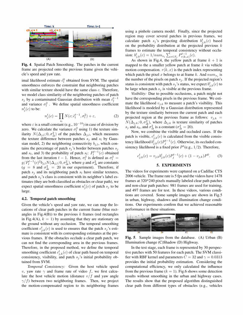
Fig. 4. Spatial Patch Smoothing. The patches in the currentframe are projected onto the previous frame given the vehi-cle’s speed and yaw rate.

imal likelihood estimate c0l obtained from SVM. The spatialsmoothness enforces the constraint that neighboring patcheswith similar texture should have the same class c. Therefore,we model class similarity of the neighboring patches of patchsj by a contaminated Gaussian distribution with mean ct−1

l

and variance �2l . We define spatial smoothness coefficient

ntj(c) to be:

ntj(c) =∏sl

N(c; ct−1l , �2

l ) + ", (2)

where " is a small constant (e.g., 10−10) in case of division byzero. We calculate the variance �2

l using 1) the texture sim-ilarity N(Δj,l; 0, �2

Δ) of the patches Δj,l, which measuresthe texture difference between patches sj and sl by Gaus-sian model, 2) the neighboring connectivity bj,l, which con-tains the percentage of patch sj’s border between patches sjand sl, and 3) the probability of patch sl: P t−1

l (c) obtainedfrom the last iteration t − 1. Hence, �2

l is defined as �2l =

g/P t−1l (c)2bj,lN(Δj,l; 0, �2

Δ), where g and �2Δ are constants

(g = 8 and �2Δ = 20 in our experiment). Therefore, if

patch sj and its neighboring patch sl have similar textures,and patch sj’s class is consistent with its neighbor’s label es-timates (they are both classified as obstacles or clear path), weexpect spatial smoothness coefficient ntj(c) of patch sj to belarge.

4.2. Temporal patch smoothingGiven the vehicle’s speed and yaw rate, we can map the lo-cations of clear path patches in the current frame (blue rect-angles in Fig.4(B)) to the previous k frames (red rectanglesin Fig.4(A), k = 1) by assuming that they are stationary onthe ground without any occlusion. The temporal smoothingcoefficient ctj,k(c) is used to ensures that the patch sj’s esti-mate is consistent with its corresponding estimates at the pre-vious frames. If the obstacles occlude a clear path patch, wecan not find the corresponding area in the previous frames.Therefore, in the proposed method, we define the temporalsmoothing coefficient ctj,k(c) of clear path based on temporalconsistency, visibility, and patch sj’s initial probability ob-tained from SVM.

Temporal Consistency: Given the host vehicle speedv, yaw rate and frame rate of video f , we first calcu-late the host vehicle motion (distance v/f and yaw angle /f ) between two neighboring frames. Then, we projectthe motion-compensated region to its neighboring frames

using a pinhole camera model. Finally, since the projectedregion may cover several patches in previous frames, wecalculate patch sj’s projecting distribution btj,k(c) basedon the probability distribution at the projected previous kframes to estimate the temporal consistency without occlu-sion: btj,k(c) = 1/numsj

∑x∈Sj

P t−1r(k,x)(c).

As shown in Fig.4, the yellow patch at frame k + 1 ismapped to the a smaller yellow patch at frame k via vehiclemotion compensation. r(k, x) is the patch index representingwhich patch the pixel x belongs to at frame k. And numsj isthe number of the pixels on patch sj . If the projected region’sstatus is consistent with patch sj’s status, we expect btj,k(c) tobe large when patch sj is visible at the previous frame.

Visibility: Due to possible occlusions, a patch might nothave the corresponding pixels in the previous frame. We esti-mate the likelihood vj,k to measure a patch’s visibility. Thislikelihood is modeled by a Gaussian distribution representedby the texture similarity between the current patch and eachprojected region at the previous frame as follows: vj,k =N(Δj,k; 0, �2

Δ), where Δj,k is texture similarity of patchessj and sk, and �2

Δ is a constant (�2Δ = 20).

Now, we combine the visible and occluded cases. If thepatch is visible, ctj,k(c) is calculated from the visible consis-tency likelihood btj,k(c)P t−1

j (c). Otherwise, its occluded con-sistency likelihood is a fixed prior P t(e.g., 1/2). Therefore,

ctj,k(c) = vj,kbtj,k(c)P t−1

j (c) + (1− vj,k)P 0. (3)

5. EXPERIMENTSThe videos for experiments were captured on a Cadillac CTS2006 vehicle. The frame rate is 5 fps and the videos have 1478frames at 320*240 pixels manually labeled clear path patchesand non-clear path patches: 981 frames are used for training,and 497 frames are for test. In these videos, various condi-tions are covered. Some sample images are shown in Fig.5in urban, highway, shadows and illumination change condi-tions. Our experiments confirm that we achieved reasonableperformance in these situations.

Fig. 5. Sample images from the database. (A) Urban (B)Illumination change (C)Shadow (D) Highway.

In the test stage, each frame is represented by 30 perspec-tive patches with 50 features for each patch. The SVM classi-fier with RBF kernel and parameters C = 32 and = 0.0313provides the initial probability estimation. Considering thecomputational efficiency, we only calculated the influencefrom the previous frame (k = 1). Fig.6 shows some detectionresults without smoothing in the urban and highway cases.The results show that the proposed algorithm distinguishedclear path from different types of obstacles (e.g., vehicles

Fig. 6. Result of initial detection using SVM

or road-side) without any smoothing. However, SVM-basedapproach wrongly classified lane-markers as non-clear pathas shown in Fig.7(A). Furthermore, in the challenging casesas shown in Fig.7(A,2) and Fig.7(A,3), the bridge’s shadowand illumination change influenced a patch’s texture causinga wrong decision. We applied spatial and temporal smooth-ing to further improve the detection performance. Fig.7(B)demonstrates the results after smoothing. For example, thewrongly classified patch in Fig.7(A,1) was corrected by thespatial smoothing of its neighboring patches. The wronglyclassified patches in Fig.7(A.2) and (A.3) were corrected bythe temporal and spatial smoothing of neighboring patches.

Fig.8 summarizes the performance of clear path detectionwith and without smoothing using ROC curve. Comparedwith SVM classification which had 92.23% in accuracy (thenumber of correctly classified patches / the number of totalpatches), 4.6% in FAR (False Alarm Rate) and 5.1% in FRR(False Rejection Rate), additional patch-based smoothing im-proved the accuracy to 94.57% and reduced FAR to 3.2% andFRR to 4.5%. Additional results are shown in Fig.9 whichdemonstrates our method performing well in various scenar-ios such as urban, countryside and highway.

Fig. 7. Patch-based smoothing

Fig. 8. Comparison of clear path detection

6. CONCLUSIONSTraditional methods for autonomous driving detect all objectsin the scene, and infer the remaining areas as clear path. How-ever, such a system, which requires multiple object detectors,is complex, slow and not very reliable.

Fig. 9. Additional results in various scenarios

In this paper, we proposed a method to detect clear pathdirectly in the scene only using one clear path detector andshowed that it performed robustly even in some challengingsituations with shadows and illumination changes via spatialand temporal smoothing.

7. REFERENCES

[1] S. Sugimoto, H. Takahashi, and M. Okutomi, “Obstacledetection using millimeter-wave radar and its visualiza-tion on image sequence,” IEEE international Conferenceon Pattern Recognition, pp. 342–345, 2004.

[2] C. Wang, C. Thorpe, and A. Suppe, “Ladar-based detec-tion and tracking of moving objects from a ground vehi-cle at high speeds,” IEEE Intelligent Vehicles Symposium,2003.

[3] M. Salinas, E. Rafael, and F. Aguirre, “People detectionand tracking using stereo vision and color,” Image VisionComputing, pp. 995–1007, 2007.

[4] I. Alonso, D. Llorca, and M. Garrido, “Combination offeature extraction methods for svm pedestrian detection,”IEEE Transactions on Intelligent Transportation Systems,pp. 292–307, 2007.

[5] D. Ramanan, D. A. Forsyth, and A. Zisserman, “Trackingpeople by learning their appearance,” IEEE Transactionson Pattern Analysis and Machine Intelligence, pp. 65–81,2007.

[6] P. Viola and M. Jones, “Rapid object detection using aboosted cascade of simple features,” IEEE Computer So-ciety Conference on Computer Vision and Pattern Recog-nition, p. 551, 2001.

[7] D. Karuppiah P. Silapachote and A. Hanson, “Featureselection using adaboost for face expression recognition,”International Conference on Visualization, Imaging, andImage Processing, p. 551, 2004.

[8] T. F. Wu, C. J. Lin, and R. C. Weng, “Probability esti-mates for multi-class classification by pairwise coupling,”Journal of Machine Learning Research, pp. 975–1005,2004.