campaign spending and electoral competition: towards · pdf filecampaign spending and...

CFI/BPC Working Group on Money-in-Politics Research Agenda 1

Campaign Spending and Electoral Competition:

Towards More Policy Relevant Research

Jeff Milyo

University of Missouri

[email protected]

Final draft of paper to be published in

The Forum: A Journal of Applied Research in Contemporary Politics

Volume 11, Issue No. 3 (October 2013), p. 437-454.

Please note that this is a final draft submitted to The Forum, subject to slight last

minute editing by The Forum. Consult the published version for exact quotations.

This paper is one of a series commissioned as part the Campaign Finance Institute/Bipartisan Policy Center

Working Group on Money in Politics Research Agenda.

For more on the working group and to see other papers, visit:

http://www.cfinst.org/moneyandpolitics_scholarsAgenda.aspx


Campaign Spending and Electoral Competition:

Towards More Policy Relevant Research1

Jeff Milyo

University of Missouri

[email protected]

Abstract

There is a long-standing scholarly literature on the electoral effects of campaign spending; nevertheless, the academic research offers only limited guidance for policy makers interested in campaign finance reform. In part, this is because existing studies have focused narrowly on some vexing statistical issues, while ignoring many others. But it is also because political scientists have not devoted enough effort conducting evaluation studies of how regulatory policies impact the intermediate goal of competition, let alone the ultimate policy goals of reduced corruption, increased citizen participation and improved public policy. Consequently, there is a great need for updated and improved analyses of the treatment effect of campaign spending on political competition in a variety of electoral contexts, but an even greater need for the application of modern evaluation methods to the more basic question of whether campaign finance reforms “work” as advertised.

Key Words: Campaign Spending, Political Competition, Campaign Finance Reform

Bio: Jeff Milyo is a Professor of Economics at the University of Missouri and a Senior Fellow at the Cato Institute. His recent research examines the causes and consequences of political corruption and the efficacy of state regulations on campaign financing, grass roots issue advocacy, and voter identification.

1 An earlier version of this draft was presented to the CFI-BPC Money in Politics Research Advisory Group meeting

in Washington, DC (February 22, 2013) with financial support from the Omidyar Network. I also gratefully acknowledge helpful comments from all of the working group participants and in particular, Don Green and Michael Malbin.


1. Introduction:

Political scientists, economists and other social scientists have studied the electoral

effects of campaign spending with such intensity over the past several decades that it would be

quite reasonable to expect severely diminishing returns from further research on the subject. A

logical corollary to this conjecture is that scholars should by now be able to analyze and

recommend campaign finance regulatory policy with great confidence. However, I contend that

both accounts are far from true. This not to say that there is a shortage of confidently expressed

expert opinions on campaign finance reform; only that such advice is based on a surprisingly

limited foundation of well-tested and well-understood scientific evidence. And while this

diagnosis applies to the study of money in politics in general, in this essay, I will focus only on

issues most directly related to campaign spending and political competition.

The past thirty years of research on campaign spending and political competition have

trod a narrow path. Early research on campaign spending examined candidate vote shares in

Congressional elections under some simple but defensible maintained assumptions; at the time,

scholars were striving to answer novel questions with limited data, so did the best they could.

These studies produced puzzling results and as is often the want among academics, subsequent

efforts have focused inwardly on explaining these early findings to the detriment of addressing

more substantive questions that have arisen about the role of money in politics. Empirical

researchers have been so enthralled by the methodological challenge of identifying the causal

effect of candidate campaign spending in Congressional elections under the same maintained

assumptions, that comparatively little attention has been devoted to other electoral contexts or to

wrestling with several other pesky but largely unacknowledged methodological challenges.

Some of the fundamental methodological issues that this field of research has ignored or

downplayed include: defining and measuring political competition in a meaningful way, the

potential spillover effects of campaign spending in concurrent races, and the fact that candidate

emergence is itself a function of the expected electoral conditions, to name just a few. At the

same time, scholars have devoted too little attention to conducting rigorous evaluation studies of

policy reforms to campaign finance regulations. As a consequence, despite the long and active

tradition of research on money in politics, there remains much work to be done.


The purpose of this essay is not to catalogue all of the research that has been done on the

subject of campaign spending and competition; reviews of that sort have been done before, most

recently by Stratmann (2005). Rather, the goal of this essay is to characterize the current best

practices in the scholarly literature, explain how this research informs public policy and what

directions future research must explore in order to better inform policy.

2. Why Do We Care About Political Competition?

We don’t care about competition, not for its own sake at least. Political competition, like

market competition, is just a means to some end; there is nothing more to commend it. In

economics, competition is often --- but not always --- a process that leads to greater efficiency

and economic growth. Similarly, political competition should be thought of as an intermediate

or instrumental goal; it may lead to more faithful representation, better policy outcomes, less

corruption, or greater citizen engagement. But policies directed at increasing competition for

competition’s sake may have unintended or perverse consequences, whether in economics or

politics.

For example, term limits may stimulate increased competition for seats in the legislature,

but legislative term limits also may exacerbate the already notoriously short time horizon of

elected officials and undermine their incentives for developing policy expertise. Similarly,

public financing of campaigns may increase the numbers of hapless challengers, while de-

legitimizing the few high-spending candidates that actually might have a chance to unseat an

incumbent. And open primaries may make it more difficult for parties to select their best

qualified candidate to run in the general election. But who knows how any of these reforms

ultimately impact public policy and the integrity of democracy?

Political reforms, whether in campaign financing, the primary process, term limits, etc.

are typically sold to the public as means to increase competition with the presumption that this in

turn will yield positive dividends in the form of improved public policy, less corruption and

greater civic engagement. And while it is more often than not a fascinating exercise for

researchers to explore the consequences of various reforms on political competition, what is

sorely lacking in the scholarly literature are true evaluation studies that examine the

consequences of reform on the ultimate outcomes of interest that affect citizens well-being, such

as corruption, growth, liberty, and so on. Only recently have scholars begun to exploit the


natural experiments offered by the existence of different campaign finance regulatory regimes

across the states for the purpose of evaluating reform proposals; the first and foremost call for

future research is for more work along these lines.2

Nevertheless, there is still good reason to consider the effects of campaign spending on

electoral competition. For one, specific knowledge about the “production function” for votes

and whether it is different for different types of candidates, or across different types of races may

be useful for setting public financing subsidies or even contribution limits. For one thing, it

really has been the primary focus in the scholarly literature. For another, the marginal

production of campaign spending tells us something about how grateful or likely to be influenced

a candidate may be by a monetary contribution or even outside spending. Consequently,

research on how campaign spending affects competition is valuable, but scholars should not be

so exclusively obsessed with the intermediate goal of political competition; our ultimate policy

concern is with the well-being of citizens.

3. Electoral Effects of Campaign Spending: Is there a Consensus?

Yes, there is something of a scholarly consensus, at least for campaign spending in

congressional races. However, this consensus stands in stark contrast to the popular wisdom so

often echoed by pundits, politicians and reform advocates that elections are essentially for sale to

the highest bidder (spender). Decades of social science research consistently reveal a far more

limited role for campaign spending. Early studies tended to find that spending by challengers

was far more effective than incumbent spending. More recent work argues that in principle

campaign spending is equally productive across candidates, but that there are strongly

diminishing marginal returns to campaign spending. Since most challengers spend less than

incumbents, their spending is marginally more effective, even though the underlying “production

function” that transforms money into votes is not different for challengers. Further, the best

efforts at identifying the treatment effect of money in congressional races yield fairly similar

substantive results: candidate spending has very modest to negligible causal impact on candidate

vote shares.

2 E.g., for evaluations of the effects of state campaign finance reforms on corruption, perceptions of corruption and trust in government, see: Primo and Milyo (2006), Milyo (2012) and Cordis and Milyo (2013). For evalutions of the effects of state reforms on electoral competitiveness, see: Primo, Milyo and Groseclose (2006), Stratmann (2010) and Stratmann and Aparicio-Castillo (2006).


In the next section, I discuss in more detail three noteworthy studies that represent the

frontier of methodologically sound attempts to estimate the treatment effects of campaign

spending in Congressional elections (Levitt 1994, Gerber 1998 and Stratmann 2009). But before

wading into a discussion of statistical methodology, I first demonstrate that these studies all yield

similar substantive results despite employing very different methods and data sets. To show this,

I take the point estimates for the effects of incumbent and challenger spending from each study

and generate predicted effects for increments to spending in the 2012 general elections to the

U.S. House. Both Levitt (1994) and Stratmann (2009) study House elections, so their results

translate smoothly to 2012 with only some adjustment for inflation. Gerber (1998) examines

Senate elections, but he models campaign spending per voter, so his results are also easily

applied to House districts, as well.

The preferred estimates from these studies are based on non-linear models that relate the

natural logarithm of challenger and incumbent spending to percentage vote shares. In order to

compare the effects of an increase in campaign spending using estimates from a non-linear

model, it is necessary to specify a baseline. For this, I choose the 76 most competitive House

races in which either the incumbent garnered 55% of the vote or less, or for open seats, in which

the winner received 55% of the vote or less.3 In these races, average candidate spending was

about $2.6 million for the incumbents, just over $1.7 million for challengers and about $1.5

million for open seat candidates. But that is not the full story. In these most competitive races

outside groups were quite prominent, spending on average another $2 million on behalf of

incumbents, $2.2 million on behalf of challengers and $3.2 million in open seat contests.

These facts introduce an obvious difficulty: previous studies of the effects of campaign

spending consider only candidate expenditures. Until recently, outside spending of these

magnitudes was not a frequent occurrence, so simply not a concern of researchers studying the

effects of campaign spending. Is spending by non-candidate groups as effective as candidate

spending? Quite possibly not, since such spending is not coordinated by candidates themselves,

but the extent to which outside spending substitutes for candidate spending is an open question

and a high priority for future research. For the sake of this example, and as a reasonable first

3 Data on spending and vote margins are from the Campaign Finance Institute: http://www.cfinst.org/Press/PReleases/12-11-09/Early_Post-Election_Look_at_Money_in_the_House_and_Senate_Elections_of_2012.aspx


pass, I will simply add outside expenditures on behalf of candidates to the candidate spending

totals.

A second difficulty arises from the fact that of the three studies only Levitt (1994)

explicitly estimates the effect of candidate spending in open seat races. However, since all three

studies find that equal levels of candidate spending are in principle equally productive (i.e., the

production function is similar across candidates), I employ the average point estimate for

candidate spending from each study and apply it to each type of candidate. But since candidate

spending levels vary across incumbents, challengers and open seat races, the estimated marginal

effect of a common increment to campaign spending will nevertheless vary by candidate type.

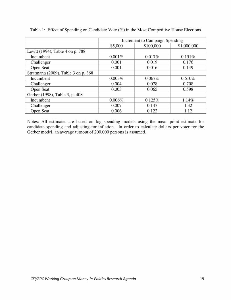
As shown in Table 1, all three studies generate similar substantive estimates for the

increased spending from a maximum $5,000 PAC contribution: in each model that additional

spending would yield at most only a few thousandths of a percentage point in vote share for any

type of candidate. Taken at face value, this suggests that House candidates should not be much

influenced by marginal PAC contributions, since the added spending has such a negligible

impact on an electoral outcome. However, if we consider much larger increments to spending

the differences in these estimates blows up. At the extreme, a hypothetical million dollar bump

in campaign spending (of the sort that might result from the activities of an outside group)

generates an estimated increase in candidate vote percentages that ranges from about 0.1

percentage points to 1 percentage point. The variation in the predicted effect of large amounts of

spending across models also begs for a horse race among competing approaches to modeling the

effects of campaign spending.

[TABLE 1 GOES ABOUT HERE.]

Even so, these predictions are well shy of what the popular wisdom might suggest, as

well as lower than the contemporaneous estimates made by the authors of these studies. This is

because as real campaign spending has increased over time, the implied marginal effectiveness

predicted by these models declines, since they are based on the natural logarithm of spending.

This underscores the need to replicate these studies with more recent data. For example, if the

technology of campaigning has improved over time, then the productivity of marginal spending

will be understated in Table 1. Likewise, if outside groups learn by doing, then we might expect

their spending to become more effective over time, as well.


In the next section, I review the current “best practices” in estimating treatment effects of

campaign spending on competition. I then discuss several remaining challenges to this genre of

empirical work, as well new directions for future research.

4. Studies of Spending and Competition in Congressional Elections

The canonical approach to studying the electoral effects of campaign spending has been

to examine general elections to the U.S. House of Representatives. Early studies made use of

newly available data on campaign spending in federal elections; this limited the number of

election cycles that could be examined. Together with the high re-election rate of incumbents,

this necessitated using vote shares as the dependent variable of interest (since there was no

meaningful variation in win rates). As a result, the following stylized model of campaign

spending and electoral competition has been the basis for essentially all subsequent analyses:

(1) Vi = β0 + β1LOG(INCSPENDi) + β2LOG(CHALSPENDi) + f1(Xi) + εi;

where:

V = incumbent vote share (%)

INCSPEND = Incumbent campaign expenditures

CHALSPEND = Challenger campaign expenditures

f1(Xi) represents exogenous control variables

and i = 1 to n, for all incumbents running and challenged for re-election.

Below, I will have more to say about some of the shortcuts embodied in this model and in the

often unstated shortcuts that empirical researchers have taken in estimating the stylized model.

But for now, all such concerns are placed aside.

As most readers are likely aware, ordinary least squares regression results for this stylized

model will likely yield a substantively large and statistically significant estimated coefficient for

challenger spending with the expected sign (β2<0). But incumbent spending will be smaller;

most likely not statistically significant and possible with an unexpected sign (β1<0). The naïve

interpretation that incumbent spending is ineffective or even counter-productive for incumbents’

electoral success has been well-understood to be the product of “endogeneity bias.” This is

because candidate spending is not determined independent of candidate vote shares as implied by

this simple model. Thus this model violates a basic assumption of the ordinary least squares

estimation method. This realization motivated several early studies to consider tweaking the


stylized model so as to get the “right” coefficient estimate for incumbent spending (e.g.,

Jacobson 1978 and 1985; Krasno and Green 1988 and Green and Krasno 1990).

Simultaneity Bias

The interdependence of campaign spending and vote shares may come about for a variety

of reasons. One possibility is “reverse causality” or true simultaneity; in other words, incumbent

spending is itself a function of vote shares (and likewise challenger spending). In practice, this

will occur if contributors are more likely to give money to candidates that look like they will fare

well in the general election. In this case, ordinary least squares estimation of the stylized model

will yield exaggerated effects of candidate spending (thus this concern alone doesn’t explain the

“wrong sign” on incumbent spending). Another source of simultaneous causality is the

possibility that contributors hang back expecting the incumbent to win, but when some surprise

occurs during the campaign that makes the race look closer than expected, then more money

flows to both candidates. This phenomenon would explain the perverse estimate on incumbent

spending (i.e., incumbents fare worse when spending more). But notice that in both examples,

the estimated effect of challenger spending is biased upward, as well.

Structural and Reduced Form Models

The stylized model can be extended to permit the simultaneous determination of spending

and votes shares by adding two more equations:

(2) LOG(INCSPENDi) = f2(Vi, LOG(CHALSPENDi,; Xi, Z2i ) and

(3) LOG(CHALSPENDi) = f3g(Vi, LOG(INCSPENDi,; Xi, Z3i ), where:

The Z’s represent true “exogenous” determinants of incumbent or challenger

spending; in other words, variables describing phenomena that are not also

proximate determinants of vote share.4

This new three equation system is known as a “structural model”; there are now three dependent

variables: vote share, incumbent spending and challenger spending. The coefficients of interest

in equation (1), β1 and β2, are called structural coefficients; they represent the proximate causal

effect or “treatment effect” of campaign spending on vote shares. The Z-variables in equations

4 For ease of exposition, I have compressed the representation of equations (2) and (3) using the general functional notation.


(2) and (3) are called “instrumental variables”; the existence of these instruments permits

identification of the structural coefficients in equation (1) via an instrumental variables

regression (e.g., Two-Stage Least Squares). However, several scholars argue forcefully that

most attempts at employing instrumental variables in the political science literature have

employed invalid instruments (see Levitt 1994, Gerber 1998, Erickson and Palfrey 1998).

This structural equation model can be solved to express the dependent variables as only

functions of the exogenous variables in the system:

(1*) Vi = g1(Xi, Z2i, Z3i)

(2*) LOG(INCSPENDi) = g2(Xi, Z2i, Z3i) and

(3*) LOG(CHALSPENDi) = g3(Xi, Z2i, Z3i).

These three new “reduced-form” equations may all be estimated separately via ordinary least

squares, since the right-side variables are all exogenous. The reduced-form estimated

coefficients in equation (1*) describe the net effects of changes in exogenous variables on vote

share (working through all the direct and indirect pathways that are illustrated in the structural

model above).

Milyo (2001) examines episodes of shocks to House incumbents’ campaign spending

associated with changes in committee power or federal campaign finance laws. Reduced-form

estimation reveals that these shocks do indeed produce significant increases in incumbent

spending, but no net impact on vote shares. This finding is consistent with the results of several

seminal studies that estimate the treatment effect of campaign spending via structural estimation

of equation (1), as illustrated in Table 1. Even so, structural estimation is by far the more

common approach to investigating the impacts of campaign spending on electoral competition.

Omitted Variable Bias

Early studies of the electoral effects of campaign spending focused largely on

simultaneity as the main source of endogeneity in Equation (1).5 But later studies emphasized

important unobservable determinants of both candidate spending and electoral success. For

example, candidate quality, such as whether a challenger held prior elective office is an input to

both raising money and winning votes (i.e., it is an example of an element of X in the structural

5 An extreme example is Erickson and Palfrey (1998); the authors identification strategy explicitly assumes that there are no unobserved underlying determinants of spending and vote shares.


model). Failing to control for candidate quality means that this important determinant of vote

share is left as part of the error term of the regression (the error term in a regression may be

thought of as “all other unobserved stuff”). But that would also mean that the key independent

variables of interest, candidate spending, are also determined by something in the error term,

which is a violation of the independence assumption. Again, this type of omitted variable bias

would tend to overstate the effects of candidate spending, so by itself does not correct the

frequently observed “wrong sign” on incumbent spending.

An added difficulty is that candidate quality likely consists of inherently difficult or

impossible to measure personality traits, such as competence, charisma, intelligence,

compassion, humor, etc. This means that even after researchers include controls for observed

candidate quality, there remains a serious potential for omitted variable bias from unobserved

candidate quality.

Candidate Fixed Effects

Concerns about unobserved candidate quality led Levitt (1994) to examine the effects of

changes in campaign spending on changes in electoral success for repeat meetings of the same

two candidates for a House seat. His key insight is that personality traits are fixed, so the first-

difference of equation (1) is purged of any time-invariant unobserved determinants of both

spending and vote shares. This approach yields a positive coefficient on incumbent spending

(i.e., the expected signs). In addition, the null hypothesis that spending is equally productive

across candidates cannot be rejected (i.e., β1= -β2); however, the estimated coefficients for

candidate spending are an order of magnitude smaller than studies that ignore unobserved

candidate quality; further, the candidate spending estimates are not even jointly significant (i.e.,

β1 = β2 = 0)!

Levitt (1994) posits that unobserved candidate quality is a far more important source of

endogeneity than true simultaneity, so that previous research findings were biased, but not in the

way most scholars had presumed. Instead, it is challenger spending that is biased most

dramatically upward in earlier studies. Of course, the subset of House races that involve repeat

meetings of candidates is not random, so these results are subject to selection bias. However,

Milyo (1998) confirms that the substantive implications in Levitt (1994) are robust to additional

years of data, additional control variables and attempts to control for sample selection bias.


Nevertheless, it should be emphasized that while controlling for candidate fixed effects addresses

bias from time-invariant unobservables, it does not eliminate concerns about simultaneity in the

changes in spending and vote-shares.

District Fixed Effects

Stratmann (2009) conducts an analysis of House elections that is similar in spirit to

Levitt’s, except that he estimates models with district fixed effects. While in principle it is

possible to control for socioeconomic characteristics of House districts, most studies do not.

This is problematic, since the propensity to contribute to candidates is at least partly a function of

constituents’ education, income, etc. But even if a researcher adds such controls to the elements

of X in the structural model, there will likely still be some important unobserved determinants of

both spending and vote shares, such as the cost of campaigning, local party organization, media

markets, etc. Stratmann addresses these concerns in two ways. He collects district specific

measures of advertising costs and uses this to convert campaign expenditures into standardized

“advertising units.” Stratmann also includes district-fixed effects in his regression analysis to

control for unobserved time invariant attributes of districts. The results of this exercise largely

confirm the findings in Levitt (1994): the productivity of campaign spending is similar for

challengers and incumbents, and the treatment effect of spending is quite small (see Table 1).

However, as was the case with Levitt’s model, Stratmann (2009) focuses only on unobservables

as the source of endogeneity bias.

Instrumental Variables

More often than not, researchers have employed instrumental variables to identify the

treatment effect of candidate spending on vote shares. The seminal study in this tradition is

Gerber (1998), although as noted above he examines U.S. Senate elections rather than House

elections. Gerber (1998) provides a template for researchers to follow in considering the

selection and screening of possible instrumental variables; his is the first study in this literature

to actually test the validity of commonly employed instruments using standard over-

identification tests (and finds instruments employed in previous studies to be invalid).

Gerber (1998) proposes two novel instruments for identifying the electoral effects of

campaign spending in Senate elections: candidate wealth and campaign spending in the race for


the other Senate seat in the same state. However, Gerber ignores potential omitted variable bias

from state-specific unobservable determinants of campaign spending and electoral competition

(for example, media costs and state party organization). Nevertheless, Gerber also finds that

incumbent and challenger spending are equally productive (i.e., β1 = - β2); further, the estimated

coefficients are statistically significant.

Putting It All Together?

I have identified three studies that employ “best practices” for estimating the treatment

effect of campaign spending in Congressional elections. However, each employs a different

method; an obvious task for future work would be to combine Gerber’s (1998) attention to

instrumental variables with the concern for unobservable candidate and district characteristics

shown by Levitt (1994) and Stratmann (2009). For example, it would be trivial to include state-

specific fixed effects in to Gerber’s analysis. Likewise, data on candidate wealth is now readily

available online, so could be employed as an instrument in studies that adopt models like those

used by Levitt or Stratmann.6 Given the real increase in campaign spending over time and the

rise of outside spending, there is a great need to synthesize the lessons from these studies and to

analyze more recent election data. In addition, these best practices need to be applied to the

study of state elections, judicial elections, and ballot measures; methodological rigor is no less

important in less salient races!7

5. Unaddressed Challenges

The best practices for estimating the canonical structural models of campaign spending

and political competition described above still largely ignore several challenges. In effect the

basic identification problem in this literature has proven so daunting, that scholars have been

willing to sidestep or ignore other more mundane concerns. In this section, I identify several

such concerns, in no particular order:

6 Data from financial disclosure reports are readily available from the Center for Responsive Politics at their “Open Secrets” website: http://www.opensecrets.org/. For a reduced-form analysis of the electoral effects of candidate wealth, see: Milyo and Groseclose (1999). 7 For example, Bonneau (2007) investigates campaign spending in judicial elections using lagged spending as an instrument; however, lagged spending is expected to be with unobserved district and\or candidate attributes.


Concurrent Elections

On Election Day, many different types of races are decided concurrently. But you

wouldn’t know this from the literature on campaign spending in House elections. For the most

part, scholars have ignored the context of elections. Not only might the efficacy of campaign

spending be very different depending on the number and type of elections running concurrently,

but there may be spillovers from spending in one race to another. Further, the very purpose of

campaign spending may be dramatically different up and down the ballot. For example,

candidates for higher office may focus on turning out supporters, while down ballot candidates

may focus on persuading voters that will be already intending to go to the polls in order to vote

in more prominent races. Thus for several reasons, there may be strong contextual effects from

campaign spending that have been completely ignored to date.

Measuring Competition

It has long been known that maximizing candidate vote share is not equivalent to

maximizing the probability of candidate victory.8 The same average increase in vote shares

achieved by increasing votes for woeful challengers in lopsided races versus increasing votes for

competent challengers in close races will have dramatically different implications for incumbent

turnover, tenure, possibly party control, etc. Early research on the efficacy of campaign

spending in House elections examined vote shares out of necessity, since spending data was only

recently available and most incumbents win re-election. But scholars should really be interested

in the effect of campaign spending on the probability of candidate victory, not vote shares.

Sufficient data now exists for researchers to simply substitute candidate victory for vote share as

the dependent variable of interest in the canonical model.

Measuring Campaign Spending

Most scholars measure campaign spending using the total expenditures of candidates

over the two-year electoral cycle. Of course, these totals may include spending directed at

winning a primary election; primary spending shouldn’t be counted dollar-for-dollar as general

election spending, but that’s what is done. Further, campaigns may differ in the fixed costs of

8 For a recent discussion, see Patty (2002); for an application to the effectiveness of campaign spending, see Gerber (2004).


organization or even the marginal cost of fund-raising (Ansolabehere and Gerber 1994). Finally,

there may be long-lasting effects of past campaign spending. None of these concerns has

received sufficient attention in the literature on campaign spending and competition.

The Jar of Pickles Problem

A jar of pickles costs about the same in June or October, whether in the suburbs of

Detroit or rural Kansas. The same is probably not true for the price of campaigning. In the

canonical model, electoral success is a function of campaign expenditures, but expenditures may

buy more or less campaigning as the price of campaigning varies. This concern is addressed

only by Stratmann (2009); he constructs an index of advertising costs across House districts and

uses it to translate expenditures into “advertising units.” Much more attention needs to be given

to the costs of campaigning and how it varies across districts.

The Decision to Run and Strategic Challengers

It is not random which incumbents choose to retire (e.g., Groseclose and Krehbiel 1994).

Nevertheless, the potential selection bias from incumbent retirement or lack of opposition is

almost never mentioned in studies of the effects of campaign spending. Likewise, the presence

and quality of challengers is not random. There is a substantial literature that examines

determinants of challenger entry (e.g., Krasno and Green 1988 and Goodliffe 2001), yet in the

canonical structural models, challenger presence and quality is considered to be “exogenous”

(i.e., unrelated to the context and likely outcome of the election).

Unobserved Candidate Effort

Most incumbents are electorally secure. They can afford to slack off when running for

re-election, since maximizing effort will likely increase their probability of victory only a small

amount. The problem of unobserved candidate effort is discussed at length in Milyo (2001); in

brief, the presence of unobserved candidate effort as an additional endogenous variable in the

canonical structural model means that legitimate instrumental variables no longer exist (since

unobserved effort is itself a function of all exogenous variables in the reduced-form). Again,

analyzing candidate victory instead of vote shares may mitigate the problem of unobserved

effort. However, it should be noted that even in the presence of unobserved effort, reduced form


estimates of (1*-3*) remain unbiased, although care must be taken in interpreting results, as

discussed in Milyo (2001).

6. Towards More Policy Relevant Research

The preceding section identifies several areas of improvement for future research that

otherwise hews closely to the canonical model. These suggestions are aimed at improving the

estimation of treatment effects of campaign spending on competitiveness using observational

data. Knowledge about such treatment effects can inform public policy as discussed above.

However, the many unmet challenges to identifying the causal impact of campaign spending on

electoral competitiveness should inspire great caution when it comes to informing public policy

in the present! In this section, I consider new directions for policy relevant research.

Field Experiments

Recent years have seen a renaissance in field experiments in the social sciences; in

political science, great headway has been made in our understanding of voter mobilization

(Green, McGrath and Aranow 2013). Field experiments also hold great promise for identifying

treatment effects of spending on competition, although to date much of the relevant research has

been done on low salience local elections.

Pagopoulos and Green (2008) analyze the effects of non-partisan radio ads aimed at

encouraging turnout in mayoral elections; they find these ads not only increase turnout, but lower

the margin of victory in these races. The authors suggest this is consistent with a larger impact

of advertising for challengers relative to incumbents (at the margin); however, apart from not

actually testing the effect of partisan campaign spending, the effects on vote share are not

statistically significant.

In contrast, Gerber (2004) analyzes the effects of partisan mailers in several different

types of races. In general, mailers yield positive results and imply a cost per vote roughly in line

with previous observational studies on the effects of campaign spending. However, in the one

experiment involving a general election for the U.S. House, there were no significant effects of

mailers on voting or vote shares. These results are consistent with diminishing marginal returns

to campaign spending for higher offices and\or races with more campaign spending.


Obviously, field experiments have great potential to improve our knowledge of the

treatment effects of campaign spending, as well as providing a check on the plausibility of

findings from observational data. This is an area of inquiry that merits much more effort from

researchers and encouragement from funders.

Natural Experiments

Campaign finance regulatory regimes vary considerably across state and local

jurisdictions; this variation provides a natural experiment that can be exploited to identify the

treatment effect of campaign spending on political competition. Further, to the extent these

regulations are exogenous shocks to spending; reduced-form estimation can reveal the net effects

of campaign finance reform on competition and spending, even in the presence of unobserved

candidate effort. This is the approach taken by Primo, Milyo and Groseclose (2006), Stratmann

and Aparicio-Castillo (2006) and Stratmann (2010); the former examine gubernatorial elections,

while the latter two examine state legislative elections. In both contexts, limits on contributions

from individuals reduce the winning margin for candidates.

Given these results, state campaign finance regulations provide potential instrumental

variables for identifying the effects of competition on voter turnout, trust in government, political

corruption, state tax and spending policies, etc. As noted at the start of this essay, there is no

reason to care about increasing electoral competition in and of itself. However, future research

can leverage the relationship between campaign spending and competition to identify the effects

of competition on other outcomes of interest.

Conclusion

In reviewing best practices in the estimation of the treatment effect of campaign spending

on political competition, this essay points out the strengths and weaknesses of different

approaches and the need to synthesize and update these studies. Working with existing estimates

and applying them to current data suggests that increments to spending have negligible effects on

vote shares in competitive House races. Of course, this may not be true for local or state

election, especially for lower office. Further, even this simple exercise points out the need to

better understand the efficacy of non-candidate spending in campaigns.


Future research must also take care to consider both simultaneity and omitted variable

bias and to recognize the importance of justifying and screening instrumental variables. In

addition, there is no longer a good reason to focus on vote shares as the dependent variable of

interest; nor is there any excuse for ignoring the process that determines the presence and quality

of challengers or possible selection bias from strategic retirements among incumbents. Perhaps

most importantly, the presence of unobserved candidate effort undermines any instrumental

variable approach. Reduced-form estimation holds some promise, but reduced-form models

must be derived from some underlying structural model; too often scholars estimate ad hoc

models that are impossible to reconcile as either a structural equation or a reduced-form

equation.

Field experiments hold great promise for identifying the treatment effects of spending in

specific contexts; to date, these studies produce a mix of findings. However, field experiments

on particular modes of advertising do not really test how a campaign behaves with more or less

money to spend. So while such experiments are valuable for informing campaign managers

about the efficacy of spending alternatives, they do not necessarily inform us about what

candidates would actually do with more money.

But scholars should not lose sight of the need for policy relevant research.

Understanding the electoral effects of campaign spending is just one small piece of what needs to

be done. The need for rigorous evaluation studies of campaign finance regulations and their

impact on outcomes that matter --- the quality of policy, corruption, turnout, trust in government,

etc. --- is far greater.


References:

Ansolabehere, S and Gerber, A. “The Mismeasure of Campaign Spending: Evidence from the 1990 U.S. House Elections.” Journal of Politics, 56(4): 1106-1118. Bonneau, Chris W 2007. “The Effects of Campaign Spending in State Supreme Court Elections." Political Research Quarterly 60 (September): 489-499. Cordis, A. and Milyo, J. 2013. “Do State Campaign Finance Reforms Reduce Public Corruption?” working paper, Political Economics Research Lab, University of Missouri. Erickson, R. and Palfrey, T. 1998. “Campaign Spending and Incumbency: An Alternative Simultaneous Equations Approach,” Journal of Politics, 60: 355-373. Gerber, A. 1998. “Estimating the Effect of Campaign Spending on Senate Election Outcomes Using Instrumental Variables,” American Political Science Review, 92(2): 401-411. Gerber, A. 2004. “Does Campaign Spending Work?” American Behavioral Scientist, 47(5): 541-574. Goodliffe, J. 2001. “The Effect of War Chests on Challenger Entry in US House Elections,” American Journal of Political Science, 45(4): 830-844. Green, D. and Krasno, J. 1988. “Salvation for the Spendthrift Incumbent: Re-Estimating the Effects of Campaign Spending in House Elections,” American Journal of Political Science, 32: 884-907. Green, D. and Krasno, J. 1990. “Rebuttal to Jacobson’s ‘New Evidence for Old Arguments,’” American Journal of Political Science, 34(2): 363-372. Green, D., McGrath, M. and Aronow, P. 2013. “Field Experiments and the Study of Voter Turnout,” Journal of Elections, Public Opinion and Parties, 23(1): 27-48. Groseclose, T. and Krehbiel, K. 1994. “Golden Parachutes, Rubber Checks, and Strategic Retirements from the 102d House,” 38(1): 75-99. Jacobson, G. 1978. “The Effects of Campaign Spending on Congressional Elections,” American

Political Science Review, 72: 469-491. Jacobson, G. 1985. “Money and Votes Reconsidered: Congressional Elections 1972-1982,” Public Choice, 47(1): 7-62. Krasno, J. and Green, D. 1988. “Preempting Quality Challengers in House Elections,” Journal of

Politics, 50(4): 920-936. Levitt, S. 1994. “Using Repeat Challengers to Estimate the Effects of Campaign Spending on Election Outcomes in the U.S. House,” Journal of Political Economy, 102: 777-798.


Milyo, J. 1998. The Electoral Effects of Campaign Spending in House Elections: A Natural

Experiment Approach. Citizens Research Foundation: Los Angeles, CA. Milyo, J. 2001. “What Do Candidates Maximize (and Why Should Anyone Care)?” Public

Choice, 109(1-2): 109-139. Milyo, J. 2012. “Do State Campaign Finance Reforms Increase Trust and Confidence in State Government?” working paper, Political Economics Research Lab, University of Missouri. Milyo, J. and T. Groseclose, “The Electoral Effects of Incumbent Wealth,” Journal of Law and

Economics, 42 (1999): 699–722. Panagopoulos, C. and Green, D. 2008. “Field Experiments Testing the Impact of Radio Advertisements on Electoral Competition,” American Journal of Political Science, 52(1): 156-168. Patty, J. 2002. “Equivalence of Objectives in Two Candidate Elections.” Public Choice 112(1):151-166. Primo, D. and Milyo, J. 2006. “Campaign Finance Laws and Political Efficacy: Evidence from the States,” Election Law Journal, 5(1): 23-39. Primo, D., Milyo, J. and Groseclose, T. 2006. “State Campaign Finance Reform, Competitiveness and Party Advantage in Gubernatorial Elections,” in The Marketplace of

Democracy. Eds. Michael McDonald and John Samples. Brookings Institution Press: Washington, DC. Stratmann, T. 2005. “Some Talk: Money in Politics. A (Partial) Review of the Literature,” Public Choice, 124: 135-136. Stratmann, Thomas. (2009). "How Prices Matter in Politics: The Returns from Campaign Advertising." Public Choice, 140(Issue 3-4), pp 357-377. Stratmann, T. 2010. “Do Low Contribution Limits Insulate Incumbents from Competition?” Election Law Journal, 9(2): 125-140. Stratmann, T. and Aparicio-Castillo, F.J. 2006. “Competition Policy for Elections: Do Campaign Contribution Limits Matter?” Public Choice, 127: 177-206.


Table 1: Effect of Spending on Candidate Vote (%) in the Most Competitive House Elections

Increment to Campaign Spending

$5,000 $100,000 $1,000,000

Levitt (1994), Table 4 on p. 788

Incumbent 0.001% 0.017% 0.151%

Challenger 0.001 0.019 0.176

Open Seat 0.001 0.016 0.149

Stratmann (2009), Table 3 on p. 368

Incumbent 0.003% 0.067% 0.610%

Challenger 0.004 0.078 0.708

Open Seat 0.003 0.065 0.598

Gerber (1998), Table 3, p. 408

Incumbent 0.006% 0.125% 1.14%

Challenger 0.007 0.147 1.32

Open Seat 0.006 0.122 1.12

Notes: All estimates are based on log spending models using the mean point estimate for candidate spending and adjusting for inflation. In order to calculate dollars per voter for the Gerber model, an average turnout of 200,000 persons is assumed.

campaign spending and electoral competition: towards · pdf filecampaign spending and...

Documents