Policy Research Working Paper 7516

Can a Small Social Pension Promote Labor Force Participation?

Evidence from the Colombia Mayor Program

Tobias Pfutze Carlos Rodríguez-Castelán

Poverty and Equity Global Practice GroupDecember 2015

WPS7516

Produced by the Research Support Team

Abstract

The Policy Research Working Paper Series disseminates the findings of work in progress to encourage the exchange of ideas about development issues. An objective of the series is to get the findings out quickly, even if the presentations are less than fully polished. The papers carry the names of the authors and should be cited accordingly. The findings, interpretations, and conclusions expressed in this paper are entirely those of the authors. They do not necessarily represent the views of the International Bank for Reconstruction and Development/World Bank and its affiliated organizations, or those of the Executive Directors of the World Bank or the governments they represent.

Policy Research Working Paper 7516

This paper is a product of the Poverty and Equity Global Practice Group. It is part of a larger effort by the World Bank to provide open access to its research and make a contribution to development policy discussions around the world. Policy Research Working Papers are also posted on the Web at http://econ.worldbank.org. The authors may be contacted at crodriguezc@worldbank.org.

One of the primary motivations behind the establish-ment of noncontributory pension programs is to allow beneficiaries to retire from the labor force. Yet, as with other unconditional cash transfer schemes, their aggre-gate effects may be more complex. Using panel data and instrumental variable techniques, this paper shows that the effect of one such program, Colombia Mayor, has been

to raise the labor force participation of relatively younger male beneficiaries. This increase occurred precisely in the occupations with characteristics that are likely to require some up-front investment. The paper concludes that the transfer effectively loosened the liquidity con-straints to remaining in these occupations. However, no such effect is found among women or older beneficiaries.

Can a Small Social Pension Promote Labor Force Participation?

Evidence from the Colombia Mayor Program

Tobias Pfutze1

Florida International University

Carlos Rodríguez-Castelán2

The World Bank

Keywords: Pensions, Labor Force Participation, Colombia

JEL Codes: H55, J08, J26, O15

Sector Board: Poverty and Equity Global Practice (POV)

The authors would like to thank Carlos Casteñeda, Sara Kotb, and Daniel Valderrama for helpful research assistance. This paper has benefited from helpful comments and suggestions by Wendy Cunningham, Giselle del Carmen and Robert Zimmermann. The authors are also grateful to seminar participants at the 2015 Summer Initiative for Research on Poverty, Inequality, and Gender of the Poverty and Equity Global Practice at the World Bank for their useful comments and suggestions. The authors would also like to thank Juan Carlos López and Sandra Díaz at the Colombia Mayor Implementation Agency (Consorcio Colombia Mayor), and Alejandra Corchuelo and Guillermo Rivas from the Ministry of Planning (Departamento Nacional de Planeación, DNP) for providing useful data employed for some the analysis. 1 E-mail: tpfutze@fiu.edu (corresponding author) 2 E-mail: crodriguezc@worldbank.org

2

1. Introduction Direct cash transfers have become an increasingly popular policy tool to reduce poverty in low- and

middle-income countries over the past two decades. While conditional cash transfers have made a

grand entrance in Latin America through programs such as the Bolsa Familia conditional cash transfer

program in Brazil and Progresa-Oportunidades (now Prospera) in Mexico in the late 1990s, studies have

recently questioned the conditionality aspect of the transfers and put more attention on unconditional

transfers. In particular, noncontributory pensions account for a major share of these nonconditional

transfers. In Latin America alone, 12 of 26 countries have already implemented either a

noncontributory pension or a complementary system (Bosch and Guajardo, 2012). Usually directed

toward older individuals, with an emphasis on residents of rural areas, eligible individuals receive from

as little as US$0.10 a day in Honduras to almost US$20.00 a day in Trinidad and Tobago according to

the Inter-American Development Bank (Bosch, Melguizo, and Pagés, 2013). Because these programs

do not require a contribution to a specific fund, the costliness of their implementation and their

sustainability in sometimes politically fragile developing countries have been criticized by many (Bosch

and Guajardo, 2012; Johnson and Williamson, 2006; Rofman, Apella, and Vezza, 2015).

This paper evaluates the effects of one such program, the Colombia Mayor noncontributory pension

program. This program is especially interesting because it combines two noteworthy features: it is

associated with a benefit that is quite small, and the age of eligibility is also among the lowest in such

programs in the region. We show that the program has had the effect of increasing labor force

participation in activities that can be expected to require some up-front investment for relatively young

beneficiaries who are men (in their 50s and 60s). However, no such effect is found among women.

This strongly supports the notion that unconditional cash transfer programs can expand the economic

activity of recipients by easing liquidity constraints.

The literature on the role of cash transfers in easing liquidity constraints is fairly limited. Much of the

literature on the use of cash transfers to promote entrepreneurship has focused on conditional

transfers. Gertler, Martinez, and Rubio-Codina (2006) estimate that, for every peso transferred

through Oportunidades, “beneficiary households used 88 cents to purchase consumption goods and

services, and invested the rest,” providing evidence of the use of transfers to relieve liquidity

constraints in the face of investment. Similarly, in Bolsa Família, Ribas (2014) estimates that the share

of entrepreneurs among men with low educational attainment who are beneficiaries has grown.

3

However, he questions the causal link between relieving financial constraints and the higher levels of

investment because he observes a rise in private transfers among households. In regard to

unconditional transfers or noncontributory pensions, there is evidence that supports the contribution

of pensions to relieving credit constraints as in the case of blacks in South Africa (Berg, 2013).

Moreover, the randomized control trial conducted by Haushofer and Shapiro (2013) sheds light on

how regular unconditional transfers, as opposed to lump-sum transfers, are more well suited to

encouraging long-term investment. There are four papers which are probably the closet to our study.

First, Soares, Ribas, and Osório (2010), who evaluate Brazil’s Bolsa Família and find that it raised

female labor force participation by 4.3 percentage points, even though they do not discuss this result

further. Fogel and Paes de Barros (2010) find for the same program, using aggregate data of Brazilian

municipalities, that labor force participation increased by 2-4 percentage points for males. Results for

females are also positive, yet not significant and smaller in magnitude. Next, Skoufias, Unar and

González de Cossio (2013) exploit the experimental design of Mexico’s Food Support Program

(Programa de Apoyo Alimentario, PAL) on labor supply. Although they find no significant effects of

the PAL on total labor market participation, their estimates show that PAL have a significant negative

effect on the participation of males in agricultural activities which translated into a shift into

participation in non-agricultural activities. They argue that PAL provide partial insurance (reduce

down-side risks) for food consumption that allows program beneficiaries to allocate less time into

agricultural production and more towards more risky non-agricultural activities. Finally, Martinez

(2004), in an unpublished paper, finds that Bolivia’s Bonosol Program boosted food consumption

among rural households by more than what could be purchased with the amount of the transfers. He

concludes that the additional funds are likely being used to invest in agricultural inputs.

Most other papers on the labor market impacts of noncontributory pensions find the opposite effect,

or no effect at all. A decline in overall labor supply is documented in Aguila et al. (2012) and Galiani,

Gertler, and Bando (2014), who explore pension programs in Mexico. However, the magnitude of the

decline varied considerably; it was 4.3 percentage points in Yucatan, Mexico (work for pay) (Aguila et

al. 2012), though Galiani, Gertler, and Bando (2014) find that the share of working individuals who

received benefits through Mexico’s Adultos Mayores Program fell by 20 percent after the expansion

in coverage. Other kinds of programs produce more nuanced effects. In the same Adultos Mayores

Program, Juarez and Pfutze (2015) find a reduction of similar magnitude among male recipients only,

mainly driven by poorer beneficiaries. In Mexico City, Juarez (2010) finds that the effect of a nutrition

4

transfer among seniors (Pension Alimentaria para Adultos Mayores) depends on household

composition and demographics. Past age 60, men who live in households with qualified members

retire early. However, individuals in younger age ranges increase their labor supply if they live with an

eligible man, but decrease it if they live with an eligible woman.

Maluccio and Flores (2005) also find a statistically significant negative effect of 5.5 hours worked per

week for men in response to participation in Nicaragua’s Cash Transfer Program Red de Protección Social.

Taking advantage of the initial randomized roll-out of Mexico’s PROGRESA program, Skoufias and

di Maro (2006) are not able to find any significant impact on labor force participation or leisure time.

For the case of Chile’s anti-poverty program Chile Solidario, Galasso (2006), in an unpublished paper,

does not find any consistent results for labor market outcomes.

A different labor market–related question is whether noncontributory social protection mechanisms,

of which pensions are only one type, incentivize informality. Labor force transitions between formal

and informal jobs at the margin have been documented as unintended consequences of unconditional

transfers. Following the implementation of Seguro Popular in Mexico, a shift toward informality was

undertaken by beneficiaries (Knox and Campos-Vázquez, 2010; Aterido, Hallward-Driemeier, and

Pagés; 2011; Azuara and Marinescu; 2013; Duval-Hernández and Smith Ramírez; 2011). However,

Azuara and Marinescu (2013) also find that wages have remained constant, which might suggest that

a wage differential did not elicit the shift toward informality. Similar results have also been documented

elsewhere. In Colombia, after the expansion of a public health insurance program, informal

employment rose by 2 to 5 percentage points (Camacho, Conover, and Hoyos 2014). In Argentina,

Bosch and Guajarado (2012) find that the Moratorium, a social pension program, caused women

working in formal jobs to retire earlier than they would have done otherwise. Untangling the demand

side and supply side of the labor market invites further exploration. Although there might be evidence

of less demand for formal labor among individuals receiving unconditional cash transfer benefits,

Bosch and Campos-Vázquez (2010, 1) estimate that “had the program [Seguro Popular] not been in

place, 31,000 more employers and 300,000 new formal jobs should have been registered with Mexican

social security.”

A sizable portion of the literature on noncontributory pension programs also focuses on micro level

indicators of wellbeing (see Aguila et al. 2012; Barros, Ferro, and Romero 2008; Galiani, Gertler, and

Bando 2014). In Yucatan, Mexico, noncontributory social security is associated with a decline in

5

hunger rates and a rise in medical consumption spending (Aguila et al. 2012). Similarly, in rural parts

of Mexico, Galiani, Gertler, and Bando (2014) and Salinas-Rodríguez et al. (2014) document lower

levels of depression. In Bolivia and Mexico, recipients of noncontributory social pensions were able

to raise their household consumption expenditure (Galiani, Gertler, and Bando 2014; Martínez 2004).

Beyond individual indicators, Duflo (2003) explores the effect of the recipient’s gender in South Africa

and finds that women receiving pensions are more likely to have an effect on their daughters’

nutritional status than on that of their sons. Furthermore, gender plays a secondary role in migration

whereby households with a pension-receiving member are also more likely to have a woman member

who is a migrant either for employment or to search for employment (Posel, Fairburn, and Lund

2006). Amuedo-Dorantes and Juarez (2015) and Juárez (2009) find that public transfers going to the

elderly in Mexico (noncontributory pension programs) crowd out private transfers (mostly

remittances). Their finding suggests that the effect of public transfers may extend to the support

networks of program recipients.

On the macro side, transfer programs, in general, have been studied as a potential mechanism of

inequality reduction. Gasparini and Lustig (2011, 17) estimate that, in Brazil, changes in public

transfers “explain 49 percent of the total decline in inequality.” In another paper, Lustig and Pessino

(2014) show similar results in Argentina, where the pension moratorium, introduced in 2004,

contributed to lowering the Gini coefficient by 4.2 percentage points. Equally important in

development economics is poverty reduction. In Brazil and South Africa, noncontributory social

pensions going to the elderly were found to have a significant effect on poverty reduction and

prevention as well as the prevention of the transmission of intergenerational poverty (Barrientos 2005;

Barrientos and Lloyd-Sherlock 2003).

In the next section, section 2, we give a more in-depth motivation for our study, including the

theoretical motivation. This is followed, in section 3, by a detailed description of the Colombia Mayor

Program. Section 4 describes the quality of the program’s targeting, which will lead us, in section 5, to

a discussion of the susceptibility of the program to evaluation. Section 6 describes the data used and

examines our empirical strategy, and section 7 presents our results. Section 8 concludes.

2. Motivation and Theoretical Background

6

Colombia’s noncontributory pension program features two particular characteristics that make it

worth studying. First, in comparison with other programs in the region and beyond, it offers a fairly

modest benefit. While the size of the benefit is not specifically determined by the program’s rules of

operation (it depends on the budgetary situation), official data show that, in 2012, the benefit paid

around Col$41,000 a month (about US$23 at the time). This amounts to little more than US$0.75 a

day at exchange rates or around US$1.50 a day at purchasing power parity (PPP). By comparison,

similar programs pay around US$7.00 a day PPP in Argentina, US$11.00 a day PPP in Brazil, and

US$6.50 a day PPP in Chile. Even the corresponding benefit in much poorer Bolivia pays around

US$2 a day PPP (Bosch, Melguizo, and Pagés 2013). Second, the minimum age to qualify for the

benefit is 52 for women and 57 for men, the lowest corresponding ages of eligibility in the region. In

most other countries, it is 65 or 70.

At first sight, the effect on labor market decisions of such a cash transfer to the elderly should be

straightforward. If one thinks of the impact as a simple income effect in a consumption-leisure

decision framework, recipients would be expected to work fewer hours or drop out of the labor force

altogether. As described above, several studies on similar programs have found precisely such an

effect. Yet, given the paltry amount of the benefit paid out by Colombia Mayor, it would not be

surprising if this effect were small and possibly statistically insignificant.

A different way to look at the benefit is as a constant income stream to a poor, but potentially

economically active population. Such a stream could have two effects: (a) it may act as a form of

insurance mechanism, allowing beneficiaries to engage in somewhat risky economic activities (as

interpreted by Skoufias, Unar and González de Cossio, 2013); and (b) it could alleviate the liquidity

constraints preventing beneficiaries from pursuing lucrative business or employment opportunities.

The first effect should result primarily in a shift from employment, even if under precarious

conditions, to self-employment. The second effect could result in a similar shift, but also in an increase

in labor force participation or the number of hours worked. One would anticipate the increase to be

concentrated among activities that require seed capital, such as small-scale commerce, food

preparation, or agriculture. However, it cannot be ruled out that potential beneficiaries are prevented

from taking advantage of employment opportunities if, for example, they are unable to afford

transportation costs or proper attire before the first benefit payment is received.

7

3. Description of the Program Colombia Mayor was launched in 2003 as the Programa de Protección Social para el Adulto Mayor

(PPSAM). The aim was to provide basic subsistence through noncontributory pension benefits to

elderly people who had no pension income and were living in extreme poverty. In 2010, program

administration was outsourced to the privately run Consorcio Colombia Mayor, which reports to the

Ministry of Labor. The purpose of the change was to accelerate rollout among all elderly who were

living in conditions of extreme poverty. The amount of the transfer is adjusted annually based on

budgetary considerations, but it can never exceed half the value of the minimum wage. The program

also provides a number of indirect nonmonetary benefits that are supplied through specially

established centers catering to the needs of the elderly population and administered and cofinanced

by the municipalities.

There are three main program eligibility criteria. The first is that the beneficiary must not be within

three years of reaching the official retirement age. During the period under study, this meant a

maximum age of eligibility for the benefit of 52 years among women and 57 years among men. (These

ages were subsequently raised by two years.)

The second criterion establishes that the beneficiary’s household must not score above a certain

threshold in Colombia’s system for the identification of potential social program beneficiaries (in the

Spanish acronym, Sisben). The Sisben score represents an estimate of the living conditions of

households registered in the system. It is based on information on households collected through a

system survey, including the quality of the dwelling, the number of dependents, disability status,

income, ownership of durable goods, and so on. The Sisben score is used to determine the eligibility

for all the country’s social programs at the national level. It has gone through two mayor modifications,

such that the current, third, version is usually referred to as Sisben III. Each program is associated

with a unique maximum score to identify beneficiaries. The maximum scores usually differ depending

on whether a household resides in one of the country’s 14 major metropolitan areas, in other urban

areas, or in the countryside. Moreover, for many programs, eligibility is subdivided into up to three

different levels, corresponding to different maximum scores. For prioritization purposes, Colombia

Mayor distinguishes between two levels. The maximum scores for level 1 are 36.32 for the 14 major

8

cities, 41.90 for other urban areas, and 32.98 for rural areas. For level 2 eligibility, which we use to

determine Sisben eligibility, the respective scores are 39.32, 43.63, and 35.26.

The third criterion revolves around income. It establishes that, in the case of one-member households,

a beneficiary’s income may not exceed half of a minimum wage. For beneficiaries living with other

individuals, the entire household income may not exceed one minimum wage. In the data described

below, we are able to observe how all three criteria would function; yet, we consider a potential

beneficiary eligible for the program if the age and Sisben score requirements are met. We have decided

not to impose the income criterion because it likely suffers from substantial measurement error in our

data. The income criterion is also subject to considerable changes over time. We believe, moreover,

that, given the difficulty of sorting out this criterion within the Sisben score, it is also the criterion that

is most problematic to apply in practice. In filling out the Sisben questionnaire, respondents have

perverse incentives to underreport income to qualify for various government assistance initiatives.

Adding support to these concerns, our own data show only a limited overlap between the Sisben

scores and households that are eligible based on income. The survey data employed and described in

more detail below is designed to allow construction of Sisben scores.

In addition to eligibility, the program also employs a prioritization strategy, mostly based on age, plus

other criteria, such as disability status, number of dependents, and so on. The strategy represents an

attempt to focus the program on the population 65 years of age and older. Every year, each

municipality is given a certain number of slots for new beneficiaries. If the number of eligible

petitioners exceeds the number of available slots, the prioritization strategy is intended to determine

who receives the benefit.

4. Program Targeting According to the country’s Ministry of Labor, the Colombia Mayor Program is targeted at the

protection of persons in conditions of extreme poverty (Colombia, Ministerio de Trabajo 2013). It is

of interest to study not only the program’s impact on beneficiaries, but also the extent to which these

correspond to the group at which the benefit is targeted. We start by comparing our aggregate data

with the data published by the government. According to the Ministry of Labor, the number of

beneficiaries rose from 718,376 in December 2012 to 1,259,333 one year later (Colombia, Ministerio

de Trabajo 2014). These numbers almost perfectly coincide with those given to us by the Consorcio

9

Colombia Mayor, which puts them at 718,376 and 1,259,004, respectively. The data of the 2013 round

of the Encuesta Nacional de Calidad de Vida (National Survey of Quality of Life, ENCV) used in the

analysis were collected during September and October of 2013. The Consorcio Colombia Mayor also

provided us with figures for October of 2013, putting the number of beneficiaries at 1,012,724. The

numbers implied by the ENCV are a little lower, but not by much. A weighted total of the number of

beneficiaries declared by each household yields 828,738 beneficiaries. If most of the program’s

expansion occurred in the second half of the year, this calculation seems fairly reasonable.

Table 1 presents this last total, together with other estimates of the target population that are also

derived as weighted totals from the 2013 round of the ENCV. We present totals for different age-

groups and subgroups by socioeconomic status. The first age-groups refer to the minimum age of

eligibility for the program (52 or older for women, 57 or older for men), followed by the 60–65 age-

group. For socioeconomic status, we first consider whether an appropriately aged person would

qualify for the benefit based on the household’s Sisben score. We have also created indicators for

whether a household’s per capita income puts it below Colombia’s poverty line and below the extreme

poverty line (indigence). For this, we followed the Ministry of Labor’s own methodology.3 The main

insight is that the total number of the poor in each age-group is only slightly lower than the number

of people living beneath the Sisben eligibility threshold. This bodes well for the Sisben criterion in

providing a good proxy for poverty. Moreover, given the enrollment numbers supplied by the

ministry, the poor 65 years of age or older should be largely covered.

Table 1: Estimates of the Target Population according to ENCV 2013

Total beneficiaries 828,738 Age eligible Total 7,383,638 Sisben eligible 2,083,818 Poor 2,066,330 Indigent 699,141 60 years of age or older Total 4,947,172 Sisben eligible 1,669,819 Poor 1,476,454 Indigent 525,100 65 years of age or older Total 3,414,864

3 See “Estadísticas por Tema: Pobreza y Condiciones de Vida” (database) (accessed August 4, 2015), National Administrative Department of Statistics, Bogotá, Colombia.

10

Sisben eligible 1,363,200 Poor 1,059,720 Indigent 385,274

A more detailed look at the data, however, yields a more complicated picture. Table 2 shows the

distribution of all age-eligible individuals according to their eligibility by the Sisben criterion and their

poverty status. The shares represent weighted averages of each category over all survey years. While

table 1 shows that the total number of age-eligible elderly with low Sisben scores is about equal to the

number of elderly living in conditions of poverty, table 2 shows that these two groups overlap only

partially. Over 35 percent of the poor are not considered eligible according to their Sisben scores. The

same is true of almost one-third of the indigent elderly.

Table 2: Comparison of Sisben Score and Poverty Status, percent

Eligibility Nonpoor Poor Nonindigent Indigent Total Noneligible by Sisben score 52.73 10.60 60.22 3.11 63.33 Eligible by Sisben score 17.71 18.96 28.62 8.06 36.67 Total 70.44 29.56 88.83 11.17

The most important question is how the eligibility criteria translate into actual receipt of the benefit.

Table 3 shows the share of individuals who report living in a household where at least one person

receives the benefit. We present weighted averages from the 2013 round of the ENCV. As can be

seen, coverage levels are fairly low in each of the target groups. Even among individuals who are older

than 65 years of age, only slightly over 50 percent of the indigent and of persons living in households

that are both poor and in Sisben groups 1 or 2 receive the benefit. Among all other groups, coverage

is significantly lower.

Table 3: Share of Beneficiaries according to ENCV 2013, percent

Age eligible 60 or older 65 or older Sisben eligible 32.44 37.20 40.69 Poor 31.85 39.91 47.88 Indigent 36.72 44.83 54.65 Sisben eligible or poor 28.69 34.80 39.92 Sisben eligible and poor 40.84 46.79 52.04

A different way to address this question is shown in table 4. Here, we look at the share of program

beneficiaries within each group in 2013. As becomes clear, almost 30 percent of the beneficiaries did

not fulfill the Sisben requirement, and almost 40 percent are not poor in monetary terms. While only

11

48 percent are both poor and below the Sisben threshold (which should be close to the actual eligibility

requirement), more than 15 percent of the beneficiaries are neither.

Table 4: Share among Beneficiaries in Groups according to the ENCV 2013, percent

Sisben eligible 71.65

Poor 60.59

Indigent 23.64

Sisben eligible or poor 84.25

Sisben eligible and poor 48.00 To obtain a better grasp of the role played by the eligibility criteria, we have run simple kernel

regressions. Figures 1 and 2 show the relationship between the actual receipt of the program benefit

by an age-eligible person and the household-level Sisben III score. Figure 1 shows the regression for

each year, and figure 2 the pooled results across all years, but by area. The threshold values are 39.32

for residents of the 14 major cities, 43.63 for residents of other urban areas, and 35.26 for rural areas.

Figure 1: Kernel Regression of Program Receipt on the Sisben Score, by ENCV Round

12

Figure 2: Kernel Regression of Program Receipt on the Sisben Score, by Place of Residence, Pooled across ENCVs 2010–13

This result is not surprising considering how the Sisben is administered. The Sisben interviews are

carried out by the municipalities. While the responses are tallied centrally and the formula for

calculating the score is secret, the municipality administrations have a clear interest in raising the

number of social program beneficiaries in their constituencies. Camacho and Conover (2011) have

analyzed the problem clearly. They show that the municipal authorities time the Sisben interviews

during the electoral cycle. More importantly for the present case, when the formula for an older

version of Sisben became publicly known, the distribution of the scores started to develop a

discontinuity exactly at the (then universal) cutoff level for social programs, bringing more applicants

into the program. Even if the formula is secret, local authorities should be able to gauge the probability

of falling below the eligibility threshold based on their own experience (the final Sisben score is

observable to the household). The interviews can then be manipulated accordingly because how each

variable affects the overall score should be clear.

In figure 3, we present the results of a similar exercise on household per capita income in the 2013

ENCV round. To avoid the long tail of high incomes, we have included only households with a per

capita income of up to Col$1,000,000 a month (around US$400 at exchange rate values). This leaves

13

out less than 10 percent of our sample. As with the case of the Sisben score, no clear cutoff area can

be defined. Rather, the probability of program receipt declines continuously and stays positive well

into fairly high incomes. The actual poverty lines differ by region and municipality, reflecting

differences in the cost of living. However, in 2013, they ranged roughly between Col$140,000 and

Col$240,000. The corresponding line for indigence was between Col$77,000 and Col$100,000. As is

apparent in the graph, there is a high probability of program receipt up to about twice the highest

poverty line. And this probability seems to stay positive throughout.

Figure 3: Kernel Regression of Program Receipt on Per Capita Household Income, Pooled

ENCV 2010–13

5. Evaluating the Program Colombia Mayor presents a number of formidable obstacles in a rigorous ex post impact evaluation,

all of which may be reduced to the lack of a clearly identifiable control group. In this section, we

discuss three possible approaches that, based on the program design, seem feasible, but turn out not

to be so.

In theory, the Sisben eligibility criterion should be amenable to evaluation through an identification

strategy involving a comparison across households within some range to the left and right of the cutoff

in a design inspired by regression discontinuity (RD). Given the discussion in the previous section, it

14

should come as no surprise that this approach does not prove to be fruitful. However, even without

such knowledge, we would not necessarily believe that the cutoff is followed strictly (as in a sharp RD

design) because there may be differences between the ENCV data and a household’s characteristics

at the time of the Sisben interview. (For instance, the program benefit may have lifted a marginal

household across the eligibility line.) However, this would not pose any major problems as long as the

probability of program receipt were still to change discontinuously at the cutoff (as in a fuzzy RD

design). A couple of unpublished working papers on the predecessor of Colombia Mayor, the

Programa de Protección Social al Adulto Mayor, attempt an RD approach based on estimated Sisben

scores and thresholds, but do not find any results (Rubio 2014; Rubio, Hessel, and Avendano 2015).

Analyzing the effect of a different social protection program for which eligibility is based on Sisben

scores (Régimen Subsidiado, a public health insurance program), Miller, Pinto, and Vera-Hernández

(2013) use a similar strategy, but find only weakly significant results. We are able to observe the actual

Sisben scores implied by the ENCV data and find that the official thresholds are not enforced in

practice. Moreover, below, we also provide statistics on municipality-specific prioritization, which

would be the principal reason to estimate municipality-specific thresholds, and show that, at least for

Colombia Mayor, there is not a lot of variance across municipalities.

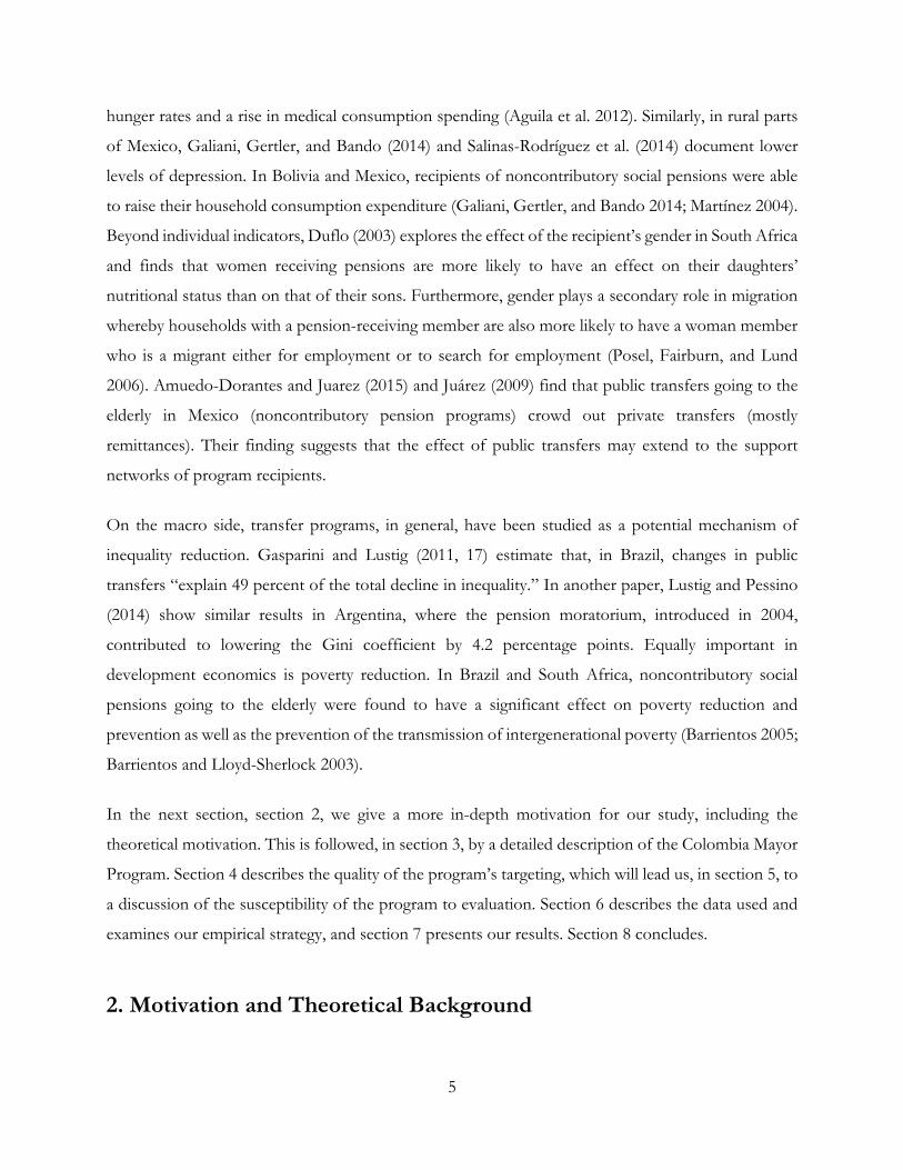
In table 5, we present the results of a simple RD-inspired spline regression with standard errors

clustered at the municipal level. We regress the binary outcome variable of a household receiving

Colombia Mayor according to whether it is Sisben eligible (another binary variable) and measure the

absolute value of its distance to the cutoff, which we capture using two separate variables depending

on whether the household is Sisben eligible (that is, to the left of the cutoff) or not (to the right of the

cutoff). In additional specifications, the squared values of these distance measures are included. This

analysis is carried out for households with at least one age-eligible member within a neighborhood of

either 5 points from the cutoff (columns 1 and 2), or 10 points (columns 3 and 4). This setup

corresponds roughly to a first-stage regression in a fuzzy RD design, and, for the approach to be valid,

one would need a strong positive effect of the binary variable Sisben eligible (which would be

interpreted as showing that the probability of program receipt changes discontinuously at the cutoff).

It can be easily seen that the variable of interest is all but insignificant statistically as well as in

magnitude. If we add the squared terms, it also becomes clear that the relation between the distance

to the threshold and actual program receipt is best captured by a linear trend. Finally, figure 4 gives a

graphical impression of the probability of receiving the benefit within the five-point window in the

15

Sisben score around the corresponding threshold value. As above, we have prepared the data using a

kernel regression. Figure 4 confirms the results shown in the table, that is, there is no significant

change around the threshold.

Table 5: RD Spline Regression of Program Receipt on Distance to the Sisben Cutoff

Dependent variable: receipt of Colombia Mayor (1) (2) (3) (4)

Within 5 points Within 5 points Within 10 points Within 10 points

Sisben eligible 0.005 0.128 0.002 0.018

(0.042) (0.157) (0.018) (0.041)

Distance to cutoff, left −0.009 0.063 −0.009*** −0.002 (0.011) (0.095) (0.003) (0.015)

Distance to cutoff, right 0.009*** 0.019*** 0.009*** 0.011*** (0.003) (0.005) (0.001) (0.004)

Distance to cutoff, left squared 0.010 0.001 (0.014) (0.001)

Distance to cutoff, right squared 0.003** 0.000 (0.001) (0.000)

Constant 0.234*** 0.227*** 0.231*** 0.232*** (0.010) (0.010) (0.009) (0.009)

Observations 10,859 10,859 21,049 21,049 R-squared 0.013 0.013 0.028 0.028 F 13.66 11.56 30.85 23.41 Note: The table shows the results of a linear probability model on a dependent variable indicating receipt of Colombia Mayor. Standard errors are in parentheses.

Figure 4: Kernel Regression of Program Receipt on Distance to the Sisben Cutoff

16

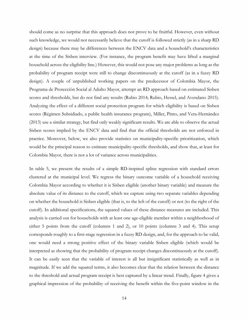
A second route to evaluation is offered through prioritization. In cases in which the number of eligible

applicants in a municipality exceeds the number of available slots in a given year, applicants are ordered

by a number of vulnerability criteria, each of which adds or subtracts a given amount to a numeric

score. Applicants with the highest such score are then enrolled first, giving rise to a municipality-

specific threshold value below which enrollment in the program is postponed. The score ranges from

a minimum of 7 to a theoretical maximum of 22. The only component that adds negative values is age

for individuals 64 years old or younger. In theory, this mechanism allows identification to be based on

a comparison between closely similar households living in different municipalities with different

thresholds. Closer examination, however, reveals that the prioritization score is only binding in a few

cases and almost only for the relatively young (that is, applicants in their 50s or early 60s), given that

age is the single most important element in the score. Table 6 shows that, of the 1,105 municipalities

on which we have 2013 prioritization data, only 78 did not apply prioritization at all. However, almost

all the other municipalities had low threshold values; the lion’s share was between −4 and −7 (a score

that can only correspond to a person in his 50s), and only 18 municipalities had a positive threshold

value. The bottom line is that the prioritization threshold does not yield sufficient variance to act as a

feasible identification strategy.

Table 6: Distribution of the Prioritization Threshold across Municipalities

Threshold value Municipalities, number Did not apply prioritization 78

−7 258 −6 267 −5 186 −4 133 −3 86 −2 42 −1 27 0 9 1 13 2 1 3 1 4 1 5 1 6 1

17

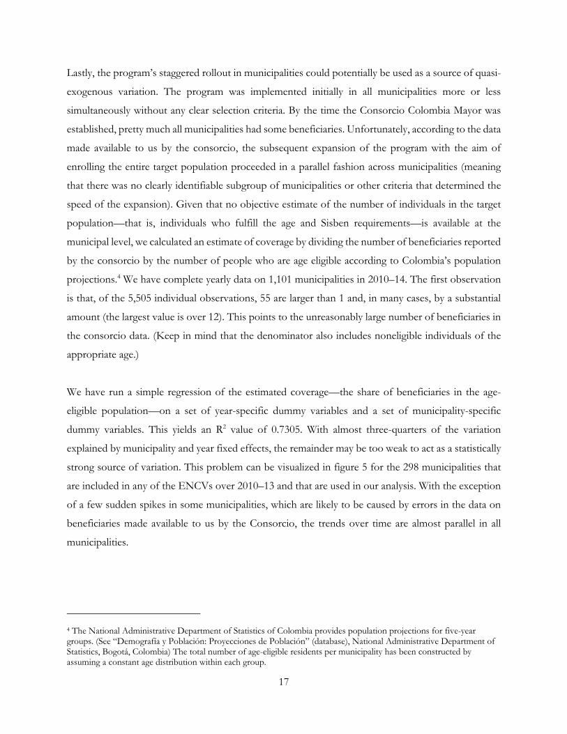
Lastly, the program’s staggered rollout in municipalities could potentially be used as a source of quasi-

exogenous variation. The program was implemented initially in all municipalities more or less

simultaneously without any clear selection criteria. By the time the Consorcio Colombia Mayor was

established, pretty much all municipalities had some beneficiaries. Unfortunately, according to the data

made available to us by the consorcio, the subsequent expansion of the program with the aim of

enrolling the entire target population proceeded in a parallel fashion across municipalities (meaning

that there was no clearly identifiable subgroup of municipalities or other criteria that determined the

speed of the expansion). Given that no objective estimate of the number of individuals in the target

population—that is, individuals who fulfill the age and Sisben requirements—is available at the

municipal level, we calculated an estimate of coverage by dividing the number of beneficiaries reported

by the consorcio by the number of people who are age eligible according to Colombia’s population

projections.4 We have complete yearly data on 1,101 municipalities in 2010–14. The first observation

is that, of the 5,505 individual observations, 55 are larger than 1 and, in many cases, by a substantial

amount (the largest value is over 12). This points to the unreasonably large number of beneficiaries in

the consorcio data. (Keep in mind that the denominator also includes noneligible individuals of the

appropriate age.)

We have run a simple regression of the estimated coverage—the share of beneficiaries in the age-

eligible population—on a set of year-specific dummy variables and a set of municipality-specific

dummy variables. This yields an R2 value of 0.7305. With almost three-quarters of the variation

explained by municipality and year fixed effects, the remainder may be too weak to act as a statistically

strong source of variation. This problem can be visualized in figure 5 for the 298 municipalities that

are included in any of the ENCVs over 2010–13 and that are used in our analysis. With the exception

of a few sudden spikes in some municipalities, which are likely to be caused by errors in the data on

beneficiaries made available to us by the Consorcio, the trends over time are almost parallel in all

municipalities.

4 The National Administrative Department of Statistics of Colombia provides population projections for five-year groups. (See “Demografía y Población: Proyecciones de Población” (database), National Administrative Department of Statistics, Bogotá, Colombia) The total number of age-eligible residents per municipality has been constructed by assuming a constant age distribution within each group.

18

This lack of municipality- and year-specific variations can be highlighted by a simple regression

analysis. Table 7 shows the result of a simple regression of the binary variable indicating receipt of

Colombia Mayor—taken from the four rounds of the ENCV during 2010–13—on the proportion of

age-eligible residents enrolled based on administrative data. The first column runs the regression using

all age-eligible observations, and the second column only shows those observations that also fulfill the

Sisben criterion (which will be the sample in our analysis below). In the first group, the municipality

proportion of beneficiaries is at least a statistically significant predictor of the actual receipt of the

benefit (at the 5 percent level, the standard errors are clustered on the municipality), but it ceases to

be a statistically significant predictor if we focus on the actual population of interest. Moreover, even

in the former group, a 1 percentage point rise in the proportion of beneficiaries would only raise the

likelihood of actual receipt by 0.173 percent. Among the second group, the corresponding likelihood

is only 0.09 percent.

Figure 5: Rollout of Colombia Mayor across 298 ENCV 2009–13 Municipalities

Table 7: Regression of Program Receipt on the Municipal Rollout Level, Controlling for Municipal and Year Fixed Effects

Binary dependent variable (1) (2)

Beneficiaries, share 0.173** 0.090 (0.073) (0.109)

Observations 48,271 20,172 R-squared 0.003 0.010 Municipalities, number 298 294 F 16.87 25.09

19

Sample Age eligible Age and Sisben eligible Note: The table shows the results of a linear probability model on a dependent variable indicating the receipt of Colombia Mayor; fixed effects are omitted from the output. Standard errors are indicated in parentheses.

There is a certain contradiction in the results arising from the last two approaches. If the rollout, that

is, the assigned number of beneficiaries, really evolved in a parallel fashion, one would expect to see

wide variation in the prioritization score of the last person entering the program because there ought

to be differences in the number and characteristics of eligible applicants. In our conversations with

officials at the consorcio, we were told that the number of assigned beneficiaries is partially adjusted

by the number of applicants a municipality is able to produce. This would explain the similarity in the

minimum prioritization scores, but it should also result in more variation in the rollout. In our

identification strategy presented in the next section, we partially assume that the official enrollment

data do not properly represent actual enrollment levels, and we proceed to derive proxies for actual

enrollment directly from the ENCV data.

6. Data and Empirical Strategy We employ the 2010–13 rounds of the yearly ENCV. The principal reason we use this particular data

source is that it provides us with the richest data in terms of variables, sample size, and periodicity.

The other frequent large-scale and nationally representative survey is the monthly Gran Encuesta

Integral de Hogares (National Integrated Household Survey). While this survey would provide us with

a much larger sample size and cover almost all the municipalities in the country, it lacks the breadth

of observed variables available in the ENCV. Most importantly, it does not capture whether a

household receives the Colombia Mayor benefit. Furthermore, the included variables do not allow for

the construction of Sisben scores.

The ENCV sampled a total of 14,801 households in 2010, 25,364 in 2011, 21,383 in 2012, and 21,565

in 2013. The sampling scheme changed in 2011 and 2012, but was held constant in 2013. The main

implication of the changes in the sampling scheme is that more municipalities are repeated in the last

two rounds than in the prior ones. This, however, has no bearing on the validity of our empirical

approach. We restrict our sample to households that have at least one eligible member according to

the age and Sisben criteria—that is, with a sufficiently low Sisben score given the place of residence—

and contain either a woman of at least 52 years of age or a man of at least 57 years of age. This yields

a total of 15,955 households (2,507 in 2010, 5,618 in 2011, 4,120 in 2012, and 3,710 in 2013). The total

20

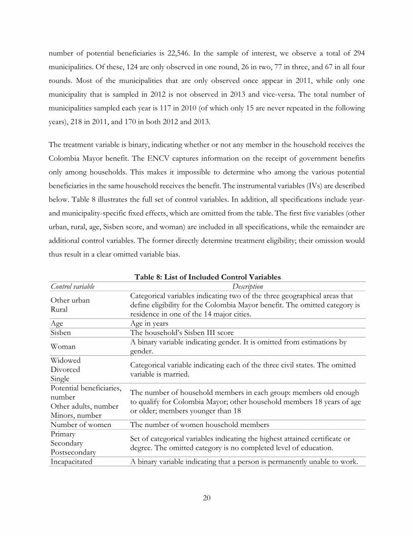
number of potential beneficiaries is 22,546. In the sample of interest, we observe a total of 294

municipalities. Of these, 124 are only observed in one round, 26 in two, 77 in three, and 67 in all four

rounds. Most of the municipalities that are only observed once appear in 2011, while only one

municipality that is sampled in 2012 is not observed in 2013 and vice-versa. The total number of

municipalities sampled each year is 117 in 2010 (of which only 15 are never repeated in the following

years), 218 in 2011, and 170 in both 2012 and 2013.

The treatment variable is binary, indicating whether or not any member in the household receives the

Colombia Mayor benefit. The ENCV captures information on the receipt of government benefits

only among households. This makes it impossible to determine who among the various potential

beneficiaries in the same household receives the benefit. The instrumental variables (IVs) are described

below. Table 8 illustrates the full set of control variables. In addition, all specifications include year-

and municipality-specific fixed effects, which are omitted from the table. The first five variables (other

urban, rural, age, Sisben score, and woman) are included in all specifications, while the remainder are

additional control variables. The former directly determine treatment eligibility; their omission would

thus result in a clear omitted variable bias.

Table 8: List of Included Control Variables

Control variable Description

Other urban Rural

Categorical variables indicating two of the three geographical areas that define eligibility for the Colombia Mayor benefit. The omitted category is residence in one of the 14 major cities.

Age Age in years Sisben The household’s Sisben III score

Woman A binary variable indicating gender. It is omitted from estimations by gender.

Widowed Divorced Single

Categorical variable indicating each of the three civil states. The omitted variable is married.

Potential beneficiaries, number Other adults, number Minors, number

The number of household members in each group: members old enough to qualify for Colombia Mayor; other household members 18 years of age or older; members younger than 18

Number of women The number of women household members Primary Secondary Postsecondary

Set of categorical variables indicating the highest attained certificate or degree. The omitted category is no completed level of education.

Incapacitated A binary variable indicating that a person is permanently unable to work.

21

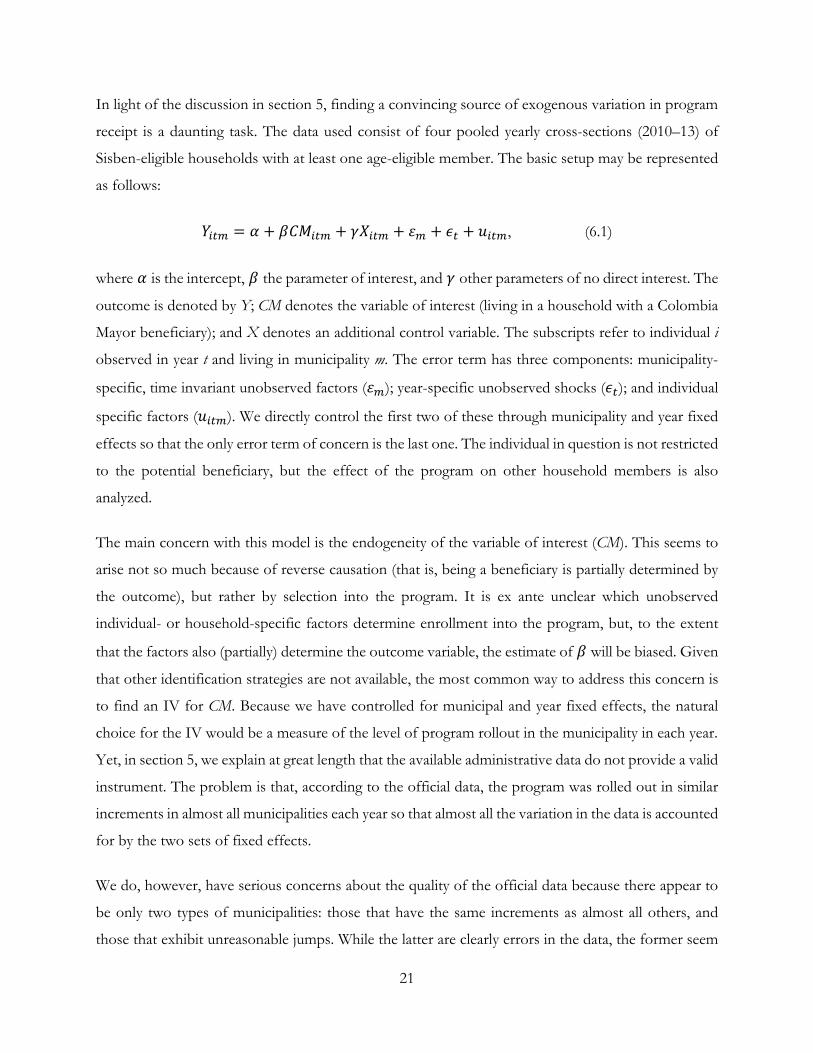
In light of the discussion in section 5, finding a convincing source of exogenous variation in program

receipt is a daunting task. The data used consist of four pooled yearly cross-sections (2010–13) of

Sisben-eligible households with at least one age-eligible member. The basic setup may be represented

as follows:

, (6.1)

where is the intercept, the parameter of interest, and other parameters of no direct interest. The

outcome is denoted by Y; CM denotes the variable of interest (living in a household with a Colombia

Mayor beneficiary); and X denotes an additional control variable. The subscripts refer to individual i

observed in year t and living in municipality m. The error term has three components: municipality-

specific, time invariant unobserved factors ( ); year-specific unobserved shocks ( ); and individual

specific factors ( ). We directly control the first two of these through municipality and year fixed

effects so that the only error term of concern is the last one. The individual in question is not restricted

to the potential beneficiary, but the effect of the program on other household members is also

analyzed.

The main concern with this model is the endogeneity of the variable of interest (CM). This seems to

arise not so much because of reverse causation (that is, being a beneficiary is partially determined by

the outcome), but rather by selection into the program. It is ex ante unclear which unobserved

individual- or household-specific factors determine enrollment into the program, but, to the extent

that the factors also (partially) determine the outcome variable, the estimate of will be biased. Given

that other identification strategies are not available, the most common way to address this concern is

to find an IV for CM. Because we have controlled for municipal and year fixed effects, the natural

choice for the IV would be a measure of the level of program rollout in the municipality in each year.

Yet, in section 5, we explain at great length that the available administrative data do not provide a valid

instrument. The problem is that, according to the official data, the program was rolled out in similar

increments in almost all municipalities each year so that almost all the variation in the data is accounted

for by the two sets of fixed effects.

We do, however, have serious concerns about the quality of the official data because there appear to

be only two types of municipalities: those that have the same increments as almost all others, and

those that exhibit unreasonable jumps. While the latter are clearly errors in the data, the former seem

22

to reflect administrative targets rather than actual enrollment levels. For this reason, we have created

two additional instruments from the ENCV data. The first attempts to replicate the level of program

rollout at the municipal level. It consists of a weighted average at the municipal level of all age- and

Sisben-eligible individuals who actually receive the benefit in each of the four years. This provides us

with an estimate of the effective year-specific level of rollout in municipalities. A second instrument

can be constructed in similar fashion at a lower level of aggregation. In addition to the location in

specific municipalities, we also observe whether a household resides in a municipality seat (cabecera),

some other urban setting (defined as anything that resembles a town), or in a dispersed rural

environment. We then construct the same weighted instrument for each of these subareas across all

four years. More formally, our instruments are as follows:

∑ (6.2)

∑ , (6.3)

where the g subscript represents the specific geographical area, and D is a specific dummy variable

indicating program participation. The two populations denoted by N include all age- and Sisben-

eligible individuals within the respective subgroups.

Neither of the two instruments is perfect on its own, and there are differences between the two. The

first is municipality and year specific. Given that we control for municipality and year fixed effects, we

are concerned with potential endogeneity because of unobserved time variant factors in the

municipalities. In terms of the empirical model presented above, the instrument may be correlated

with an additional error term, say, tm. The second instrument is constant across all four years (if it

were also year specific it would be highly collinear with the first instrument), but specific to an area at

the submunicipal level. Any endogeneity would thus derive from unobserved time invariant

characteristics that are idiosyncratic to the specific geographical group within a municipality once we

have controlled for time invariant municipal characteristics. We can think of this as an additional error

term, mg. The advantage of having two instruments available for a single potentially endogenous

variable lies in the possibility of testing for validity through an overidentification restrictions (OIR)

test, which gives us additional confidence in our strategy.

23

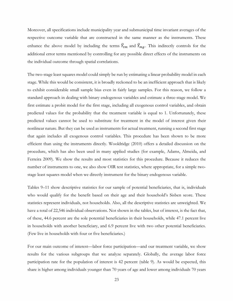
Moreover, all specifications include municipality year and submunicipal time invariant averages of the

respective outcome variable that are constructed in the same manner as the instruments. These

enhance the above model by including the terms and . This indirectly controls for the

additional error terms mentioned by controlling for any possible direct effects of the instruments on

the individual outcome through spatial correlations.

The two-stage least squares model could simply be run by estimating a linear probability model in each

stage. While this would be consistent, it is broadly reckoned to be an inefficient approach that is likely

to exhibit considerable small sample bias even in fairly large samples. For this reason, we follow a

standard approach in dealing with binary endogenous variables and estimate a three-stage model. We

first estimate a probit model for the first stage, including all exogenous control variables, and obtain

predicted values for the probability that the treatment variable is equal to 1. Unfortunately, these

predicted values cannot be used to substitute for treatment in the model of interest given their

nonlinear nature. But they can be used as instruments for actual treatment, running a second first stage

that again includes all exogenous control variables. This procedure has been shown to be more

efficient than using the instruments directly. Wooldridge (2010) offers a detailed discussion on the

procedure, which has also been used in many applied studies (for example, Adams, Almeida, and

Ferreira 2009). We show the results and most statistics for this procedure. Because it reduces the

number of instruments to one, we also show OIR test statistics, where appropriate, for a simple two-

stage least squares model when we directly instrument for the binary endogenous variable.

Tables 9–11 show descriptive statistics for our sample of potential beneficiaries, that is, individuals

who would qualify for the benefit based on their age and their household’s Sisben score. These

statistics represent individuals, not households. Also, all the descriptive statistics are unweighted. We

have a total of 22,546 individual observations. Not shown in the tables, but of interest, is the fact that,

of these, 44.6 percent are the sole potential beneficiaries in their households, while 47.1 percent live

in households with another beneficiary, and 6.9 percent live with two other potential beneficiaries.

(Few live in households with four or five beneficiaries.)

For our main outcome of interest—labor force participation—and our treatment variable, we show

results for the various subgroups that we analyze separately. Globally, the average labor force

participation rate for the population of interest is 42 percent (table 9). As would be expected, this

share is higher among individuals younger than 70 years of age and lower among individuals 70 years

24

of age or older. Also unsurprisingly, participation rates are much higher among men than among

women. Our sample consists of more women than men, especially among the relatively younger

group. This merely reflects the five-year lower minimum age for women to qualify for the benefit.

Table 9: Descriptive Statistics on Labor Force Participation

Observations, number Mean Standard deviation Minimum Maximum All 22,546 0.42 0.49 0 1 Younger than 70 All 12,644 0.53 0.50 0 1 Male 4,805 0.79 0.41 0 1 Female 7,839 0.38 0.48 0 1 70 or older All 9,902 0.28 0.45 0 1 Men 4,686 0.44 0.50 0 1 Women 5,216 0.13 0.34 0 1 Globally, with respect to the treatment variable, 26 percent of the potential beneficiaries live in

households that receive the Colombia Mayor benefit (table 10). Among household members under

70 years of age, the rate is 18 percent, whereas, among household members 70 years of age or older,

it is 37 percent. These rates are fairly consistent between men and women.

Table 10: Descriptive Statistics on Receipt of the Colombia Mayor Benefit

Labor force participation Observations, number Mean Standard deviation Minimum Maximum

All 22,546 0.26 0.44 0 1 Younger than 70 All 12,644 0.18 0.38 0 1 Male 4,805 0.17 0.37 0 1 Female 7,839 0.18 0.39 0 1 70 or older All 9,902 0.37 0.48 0 1 Men 4,686 0.36 0.48 0 1 Women 5,216 0.39 0.49 0 1

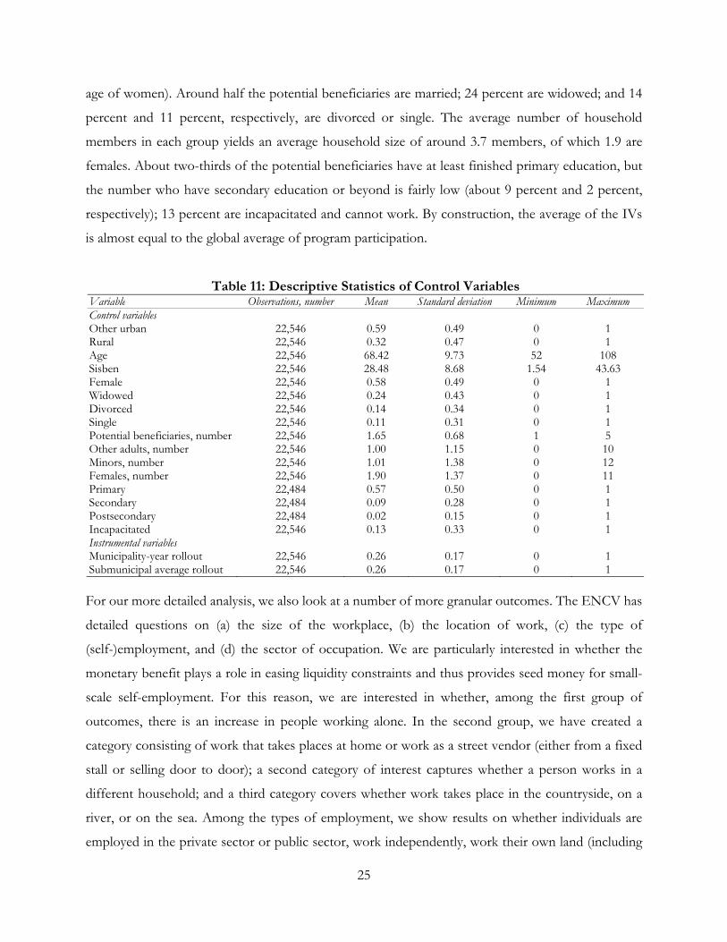
For our control variables, we present numbers only for the whole sample (table 11). A few

observations are lost because of missing values in the education-related variables. Most of our

observations are in urban areas outside the 14 major cities (59 percent), followed by individuals living

in rural settings (32 percent), which leaves a remainder of less than 9 percent who reside in one of

Colombia’s major cities. This low number mostly reflects the lower incidence of poverty in the big

cities, but also partially arises because of the stratification of the sample. The average potential

beneficiary is around 68 years old, and 58 percent are women (mainly because of the lower eligibility

25

age of women). Around half the potential beneficiaries are married; 24 percent are widowed; and 14

percent and 11 percent, respectively, are divorced or single. The average number of household

members in each group yields an average household size of around 3.7 members, of which 1.9 are

females. About two-thirds of the potential beneficiaries have at least finished primary education, but

the number who have secondary education or beyond is fairly low (about 9 percent and 2 percent,

respectively); 13 percent are incapacitated and cannot work. By construction, the average of the IVs

is almost equal to the global average of program participation.

Table 11: Descriptive Statistics of Control Variables Variable Observations, number Mean Standard deviation Minimum Maximum Control variables Other urban 22,546 0.59 0.49 0 1 Rural 22,546 0.32 0.47 0 1 Age 22,546 68.42 9.73 52 108 Sisben 22,546 28.48 8.68 1.54 43.63 Female 22,546 0.58 0.49 0 1 Widowed 22,546 0.24 0.43 0 1 Divorced 22,546 0.14 0.34 0 1 Single 22,546 0.11 0.31 0 1 Potential beneficiaries, number 22,546 1.65 0.68 1 5 Other adults, number 22,546 1.00 1.15 0 10 Minors, number 22,546 1.01 1.38 0 12 Females, number 22,546 1.90 1.37 0 11 Primary 22,484 0.57 0.50 0 1 Secondary 22,484 0.09 0.28 0 1 Postsecondary 22,484 0.02 0.15 0 1 Incapacitated 22,546 0.13 0.33 0 1 Instrumental variables Municipality-year rollout 22,546 0.26 0.17 0 1 Submunicipal average rollout 22,546 0.26 0.17 0 1 For our more detailed analysis, we also look at a number of more granular outcomes. The ENCV has

detailed questions on (a) the size of the workplace, (b) the location of work, (c) the type of

(self-)employment, and (d) the sector of occupation. We are particularly interested in whether the

monetary benefit plays a role in easing liquidity constraints and thus provides seed money for small-

scale self-employment. For this reason, we are interested in whether, among the first group of

outcomes, there is an increase in people working alone. In the second group, we have created a

category consisting of work that takes places at home or work as a street vendor (either from a fixed

stall or selling door to door); a second category of interest captures whether a person works in a

different household; and a third category covers whether work takes place in the countryside, on a

river, or on the sea. Among the types of employment, we show results on whether individuals are

employed in the private sector or public sector, work independently, work their own land (including

26

land that may be rented or sharecropped), or work without pay. We also show results on the primary

sector (including related industries), manufacturing, commerce and trade, and other services. In

addition, we present results on monthly labor income and number of hours worked. For the latter, no

information was collected in the 2012 round so that analysis on that particular outcome is excluded.

Table 12 shows the means for each of these outcomes across the various samples of interest. These

are averages across all observations, not merely the economically active. It can be seen that a

comparatively large share of each sample work alone on agricultural land, rivers, or the sea, as

independent workers, or in the primary sector. The categories associated with agricultural or livestock

activities are particularly prominent among men, who also enjoy higher incomes and work more hours.

Women are more likely to work at home, as street vendors, or in the service sector. They also account

for a much larger share of independent workers than men relative to overall participation rates. These

averages should be kept in mind in interpreting the results presented hereafter.

Table 12: Detailed Labor Market Outcomes, Means

Indicator All Younger than 70 70 or older

All Male Female All Male Female Size of business Works alone 0.24 0.30 0.42 0.23 0.17 0.25 0.09 Place of work Home or street 0.13 0.16 0.14 0.18 0.08 0.09 0.08 Other homes 0.03 0.05 0.04 0.05 0.01 0.01 0.01 Land, river, or sea 0.18 0.21 0.45 0.06 0.15 0.28 0.03 Type of occupation Private employee 0.03 0.05 0.08 0.03 0.01 0.02 0.00 Public employee 0.01 0.02 0.01 0.02 0.00 0.00 0.00 Independent worker 0.23 0.29 0.38 0.24 0.14 0.20 0.09 Own land 0.07 0.08 0.17 0.02 0.07 0.13 0.01 Unpaid 0.02 0.02 0.01 0.02 0.01 0.01 0.01 Sector of work Agriculture & related 0.19 0.21 0.46 0.06 0.16 0.29 0.04 Manufacturing 0.04 0.05 0.04 0.05 0.02 0.02 0.03 Trade & commerce 0.07 0.09 0.10 0.09 0.04 0.06 0.03 Service & tourism 0.08 0.12 0.11 0.13 0.03 0.04 0.02 Other outcomes Labor income 139,527 193,204 304,945 124,712 70,985 126,083 21,485 Hours worked 11.82 15.42 24.69 9.75 7.21 12.10 2.83

27

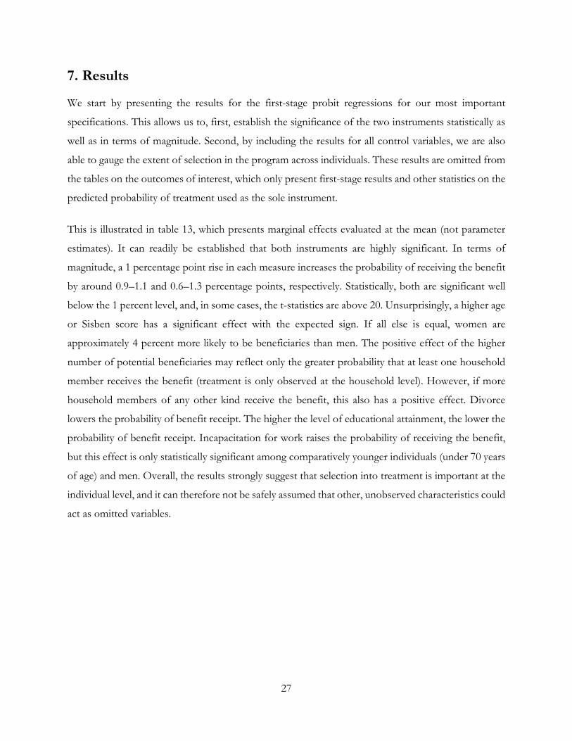
7. Results We start by presenting the results for the first-stage probit regressions for our most important

specifications. This allows us to, first, establish the significance of the two instruments statistically as

well as in terms of magnitude. Second, by including the results for all control variables, we are also

able to gauge the extent of selection in the program across individuals. These results are omitted from

the tables on the outcomes of interest, which only present first-stage results and other statistics on the

predicted probability of treatment used as the sole instrument.

This is illustrated in table 13, which presents marginal effects evaluated at the mean (not parameter

estimates). It can readily be established that both instruments are highly significant. In terms of

magnitude, a 1 percentage point rise in each measure increases the probability of receiving the benefit

by around 0.9–1.1 and 0.6–1.3 percentage points, respectively. Statistically, both are significant well

below the 1 percent level, and, in some cases, the t-statistics are above 20. Unsurprisingly, a higher age

or Sisben score has a significant effect with the expected sign. If all else is equal, women are

approximately 4 percent more likely to be beneficiaries than men. The positive effect of the higher

number of potential beneficiaries may reflect only the greater probability that at least one household

member receives the benefit (treatment is only observed at the household level). However, if more

household members of any other kind receive the benefit, this also has a positive effect. Divorce

lowers the probability of benefit receipt. The higher the level of educational attainment, the lower the

probability of benefit receipt. Incapacitation for work raises the probability of receiving the benefit,

but this effect is only statistically significant among comparatively younger individuals (under 70 years

of age) and men. Overall, the results strongly suggest that selection into treatment is important at the

individual level, and it can therefore not be safely assumed that other, unobserved characteristics could

act as omitted variables.

28

Table 13: Regression of the Treatment Variable on Instruments and Exogenous Control

Variables

Variable (1) (2) (3) (4) (5) (6) All All < 70 All >= 70 All <70 Males <70 Females

Instrument by year 0.907*** 0.890*** 0.643*** 1.155*** 0.924*** 0.887*** (0.034) (0.036) (0.035) (0.075) (0.050) (0.042)

Instrument by area 0.951*** 0.932*** 0.612*** 1.287*** 0.916*** 0.954*** (0.026) (0.028) (0.032) (0.053) (0.041) (0.038)

Other urban 0.009 0.009 0.010 0.035 0.021 0.004

(0.028) (0.024) (0.016) (0.040) (0.031) (0.034)

Rural −0.022 −0.033 −0.022 −0.013 −0.028 −0.029 (0.028) (0.024) (0.018) (0.042) (0.032) (0.033)

Age 0.011*** 0.009*** 0.012*** 0.004*** 0.010*** 0.009*** (0.000) (0.000) (0.001) (0.001) (0.001) (0.000)

Female 0.043*** 0.037*** 0.054*** 0.024* (0.006) (0.006) (0.006) (0.013)

Sisben −0.005*** −0.005*** −0.003*** −0.006*** −0.006*** −0.005*** (0.001) (0.001) (0.001) (0.001) (0.001) (0.001)

Potential beneficiaries, number 0.049*** 0.067*** 0.031* 0.062*** 0.039*** (0.013) (0.016) (0.019) (0.020) (0.014)

Other adults, number 0.047*** 0.063*** 0.027 0.071*** 0.025 (0.014) (0.015) (0.026) (0.020) (0.017)

Minors, number 0.070*** 0.054*** 0.070*** 0.086*** 0.058*** (0.016) (0.016) (0.024) (0.021) (0.018)

Females, number 0.085*** 0.116*** 0.036*** 0.100*** 0.077*** (0.009) (0.007) (0.013) (0.012) (0.010)

Widowed 0.003 0.004 −0.006 −0.005 0.007 (0.005) (0.004) (0.008) (0.006) (0.005)

Divorced −0.031*** −0.018*** −0.034*** −0.033*** −0.032*** (0.006) (0.005) (0.009) (0.008) (0.006)

Single 0.005 0.002 0.010 0.009 0.007 (0.006) (0.005) (0.009) (0.009) (0.007)

Primary −0.034*** −0.014* −0.057*** −0.030*** −0.039*** (0.007) (0.008) (0.013) (0.011) (0.010)

Secondary −0.096*** −0.042*** −0.207*** −0.052** −0.125*** (0.012) (0.011) (0.024) (0.023) (0.012)

Postsecondary −0.156*** −0.087*** −0.312*** −0.166*** −0.150*** (0.012) (0.011) (0.025) (0.016) (0.019)

Incapacitated 0.008 0.039** 0.022 0.028* −0.013 (0.009) (0.016) (0.015) (0.014) (0.013)

Observations 22,358 22,297 12,093 9,778 9,298 12,892 Note: The table illustrates a linear probability model on dependent variables indicating receipt of the Colombia Mayor benefit. Standard errors are shown in parentheses. Moving on to our actual results, we start by presenting the results for the total labor force participation

of potential beneficiaries. Table 14 has eight columns. The first four show the ordinary least squares

(OLS) regression with municipality and year fixed effects, and the second four present the IV results.

29

The first column in each groups presents the results for a parsimonious specification that includes

only a binary variable for the geographical area (other urban and rural), age, the Sisben score, and

gender as control variables. These are included because they have a direct effect on Sisben eligibility

and therefore act as omitted variables. The next column includes a full set of control variables. A

comparison of the first two columns gives, above all, an idea of the extent to which the additional

controls act as omitted variables in the first specification. This can be seen as an (imperfect) exogeneity

test on the treatment variable.

Table 14: Results for Labor Force Participation, Entire Sample

Variable (1) (2) (3) (4) (5) (6) (7) (8)

OLS OLS OLS OLS IV IV IV IV All All Males Females All All Males Females

Colombia Mayor −0.018*** −0.007 0.004 −0.003 0.069*** 0.090*** 0.116*** 0.076*** (0.006) (0.006) (0.010) (0.008) (0.017) (0.017) (0.027) (0.028)

Dependent variable by year 0.629*** 0.571*** 0.469*** 0.636*** 0.625*** 0.565*** 0.472*** 0.627*** (0.033) (0.031) (0.052) (0.045) (0.035) (0.033) (0.053) (0.047)

Dependent variable by area 0.730*** 0.679*** 0.598*** 0.668*** 0.739*** 0.691*** 0.614*** 0.669*** (0.024) (0.025) (0.045) (0.050) (0.024) (0.025) (0.047) (0.051)

Observations 22,546 22,484 9,472 13,007 22,358 22,297 9,298 12,892 R-squared 0.259 0.327 0.415 0.163 0.253 0.321 0.407 0.157 Municipalities, number 296 296 293 294 286 286 273 283 F 915.7 453.7 547.7 120.3 865.8 408.4 512.5 114.1 Partial R-squared 0.0886 0.0957 0.102 0.0951 Kleinbergen-Paap statistic 2,679 2,495 1,346 1,650 OIR test 0.358 0.358 0.786 0.0929 Endogeneity test 0.000 0.000 0.000 0.00470 First stage

Dependent variable by year 0.002 −0.000 0.006 −0.002 (0.028) (0.030) (0.044) (0.041)

Dependent variable by area −0.000 −0.001 −0.001 −0.004 (0.021) (0.023) (0.040) (0.035)

Instrument from probit 0.977*** 0.993*** 0.989*** 0.993*** (0.019) (0.020) (0.027) (0.024)

Note: The table illustrates a linear probability model on dependent variables indicating participation in the labor force. The IV specification relies on a three-stage procedure for binary treatment variables. Only the OIR test is derived from a two-step procedure. Columns (1) and (5) do not include additional control variables. Standard errors are shown in parenthesis.

The bottom of this table and of the following tables includes a number of additional statistics. While

those shown only under the OLS specification (number of observations, R2, number of municipalities,

and the F-test statistic for joint significance) should be self-explanatory, the statistics in the IV

specifications warrant additional explanation. The first two—partial R2 (Shea 1997) and the

Kleinbergen-Paap statistics (Stock, Wright, and Yogo 2002)—are weak instrument tests. Simply put,

in the case of a single endogenous regressor and no control variables, the partial R2 is reduced to the

standard R2, and the Kleinbergen-Paap is reduced to the F-test in the first-stage regression. They thus

provide measures of the magnitude and statistical significance, respectively, of the effect of the

30

instrument on the endogenous variable. It can be shown that a higher partial R2 results in a lower

asymptotic bias in the IV estimator relative to the OLS if the exclusion restriction is violated. The

Kleinbergen-Paap statistics are a panel data variant of the Cragg-Donald statistic, which has been

introduced as a weak instrument test by Stock, Wright, and Yogo (2002). Critical values for different

tests can be derived for the Kleinbergen-Paap statistic, the most conservative of which for our case

has values of around 20. Next, the OIR test allows testing for the validity of the exclusion restrictions

if the endogenous variables are overidentified (which is why we wanted to have two instruments in

the first place). The null hypothesis is that the exclusion restrictions are met, that is, the instruments

are valid. Although the test is regarded as low powered, it provides a useful check on the identification

strategy. While all the other IV-related test statistics refer to a first stage in which the sole instrument

is derived from the probit model, the OIR test is presented for a linear first stage using the two IVs

directly. Lastly, under the assumption that we have a set of valid instruments, we can test whether or

not the variable we instrumented for is indeed endogenous. The null hypothesis here is the exogeneity

of that variable.

Starting with table 15, we look at the effect of the program on the labor force participation of

beneficiaries. The important result in the first two columns is that the inclusion of the additional

control variables reduces the estimated effect of program participation by more than one-half and

reduces the significance level from 1 percent to insignificance. This is a strong indicator that the

treatment variable is endogenous and that the OLS results are likely biased. The IV results, in contrast,

are highly significant and have a positive sign. They imply that program participation has the effect of

boosting labor force participation or, probably more likely, reducing the retreat of beneficiaries from

the labor force. The likely implication of these results is that, while individuals who are not in the labor

force are more likely to receive the benefit in the first place, the actual effect of the program is that

beneficiaries tend to join the labor force. The OIR test p-values are not close to rejection of the H0,

except in the case of women, and the exogeneity of the treatment variable can be rejected.

We now analyze the counterintuitive result of an overall positive effect on the labor force participation

of beneficiaries. We start by dividing the sample into two age-groups: beneficiaries who can be

expected to be active in the labor market and beneficiaries who have probably dropped out of the

labor market because of old age. We have decided to make the cutoff at age 70. We then divide each

age-group also by gender. The first three columns of table 15 present the results for the relatively

younger cohort. The overall result is still positive, but only statistically significant among men. The

31

point estimate is much smaller among women and, hence, not significant. (The standard errors are the

same.) The next three columns show the corresponding results for individuals 70 years of age or older.

All the results are much smaller in magnitude—in the case of women, they have a negative sign—and

statistically insignificant. (Among men, the result is similar to the result among younger women.) This

establishes that the positive effect on total labor force participation is driven by beneficiaries younger

than 70, who, based on their age, can be expected to be still economically active, and, in particular, by

men.

Table 15: Results on Labor Force Participation, by Age-Group

Variable < 70 years > 70 years All Males Females All Men Women

Colombia Mayor 0.091*** 0.108** 0.066 0.008 0.060 −0.021 (0.032) (0.044) (0.044) (0.022) (0.040) (0.032)

Dependent variable by year 0.646*** 0.313*** 0.821*** 0.429*** 0.492*** 0.349*** (0.046) (0.079) (0.071) (0.056) (0.085) (0.061)

Dependent variable by area 0.713*** 0.501*** 0.792*** 0.616*** 0.676*** 0.385*** (0.049) (0.064) (0.079) (0.045) (0.077) (0.066)

Observations 12,093 3,977 7,356 9,778 4,530 5,042 R-squared 0.300 0.333 0.123 0.287 0.342 0.070 Municipalities, number 270 214 254 280 256 262 F 236.0 446.7 80.55 103.8 105.2 18.35 Partial R-squared 0.105 0.119 0.102 0.0945 0.0976 0.0917 Kleinbergen-Paap statistic 1,045 624.9 665.0 1024 495.9 721.1 OIR test 0.927 0.679 0.428 0.469 0.966 0.448 Endogeneity test 0.00702 0.0384 0.212 0.383 0.104 0.810 First stage

Dependent variable by year 0.001 0.005 −0.004 0.003 0.001 0.002

(0.042) (0.074) (0.052) (0.053) (0.070) (0.079)

Dependent variable by area 0.004 0.008 0.002 −0.001 −0.001 −0.007

(0.037) (0.060) (0.050) (0.048) (0.069) (0.087)

Instrument from probit 1.011*** 1.015*** 1.009*** 0.987*** 0.981*** 0.983*** (0.031) (0.041) (0.039) (0.031) (0.044) (0.037)

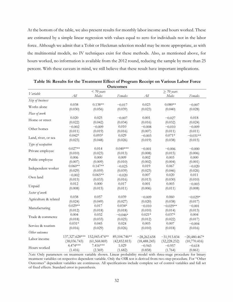
Note: The table illustrates a linear probability model relying on a three-stage procedure for binary treatment variables on the dependent variable indicating participation in the labor force. Only the OIR test is derived from a two-step procedure. All specifications include a complete set of control variables. Standard errors are shown in parenthesis. To understand the dynamics that drive the positive effect of the benefit on labor force participation,

we have to delve deeper and take a more granular look at the kind of economic activities that are

particularly affected. In table 16, we explore the results for two age-groups and for gender and

location-specific subgroups within each of these. The method employed is the same as above, that is,

we have estimated a three-stage linear probability model for the binary outcome. One could argue that

a multinomial model would be more appropriate; yet, no such models for IV estimation are available.

32

At the bottom of the table, we also present results for monthly labor income and hours worked. These

are estimated by a simple linear regression with values equal to zero for individuals not in the labor

force. Although we admit that a Tobit or Heckman selection model may be more appropriate, as with

the multinomial models, no IV techniques exist for these methods. Also, as mentioned above, for

hours worked, no information is available from the 2012 round, reducing the sample by more than 25

percent. With these caveats in mind, we still believe that these result have important implications.

Table 16: Results for the Treatment Effect of Program Receipt on Various Labor Force

Outcomes

Variable < 70 years > 70 years

All Males Females All Males Females Size of business

Works alone 0.038 0.138** −0.017 0.023 0.080** −0.007

(0.030) (0.056) (0.039) (0.023) (0.040) (0.028) Place of work

Home or street 0.020 0.025 −0.007 0.001 −0.027 0.018

(0.022) (0.042) (0.034) (0.016) (0.032) (0.024)

Other homes −0.002 −0.009 0.010 −0.008 −0.010 −0.009 (0.011) (0.019) (0.016) (0.007) (0.011) (0.011)

Land, river, or sea 0.042* 0.093* 0.029 −0.003 0.071* −0.031** (0.023) (0.048) (0.026) (0.019) (0.038) (0.015)

Type of occupation

Private employee 0.027** 0.014 0.040*** −0.001 −0.006 −0.000 (0.010) (0.023) (0.013) (0.008) (0.015) (0.006)

Public employee 0.006 0.000 0.009 0.002 0.003 0.000

(0.007) (0.009) (0.010) (0.002) (0.004) (0.001)

Independent worker 0.060** 0.147** −0.025 0.019 0.067 −0.020 (0.029) (0.059) (0.039) (0.023) (0.046) (0.026)

Own land −0.002 0.065** −0.020 0.007 0.020 0.011 (0.015) (0.033) (0.016) (0.013) (0.030) (0.010)

Unpaid 0.012 0.000 0.017 0.001 0.003 −0.003

(0.008) (0.015) (0.011) (0.006) (0.011) (0.008) Sector of work

Agriculture & related 0.038 0.057 0.039 −0.009 0.060 −0.029*

(0.024) (0.049) (0.027) (0.020) (0.038) (0.017)

Manufacturing 0.029** 0.017 0.034* −0.010 −0.029** −0.001 (0.012) (0.018) (0.018) (0.010) (0.014) (0.013)

Trade & commerce 0.004 0.032 −0.046* 0.021* 0.037* 0.004

(0.018) (0.033) (0.025) (0.012) (0.022) (0.017)

Service & tourism 0.031* 0.045 0.024 0.003 0.007 −0.004 (0.016) (0.029) (0.026) (0.010) (0.018) (0.016)

Other outcomes

Labor income 137,327.628*** 152,043.474** 89,104.746** −28,262.658 −31,913.834 −20,480.467*

(38,036.743) (61,568.069) (42,852.815) (18,488.245) (32,228.232) (10,770.416)

Hours worked 4.474*** 7.416*** 1.029 −0.943 −0.957 −0.618 (1.416) (2.369) (1.682) (0.858) (1.764) (0.861)

Note: Only parameters on treatment variable shown. Linear probability model with three-stage procedure for binary treatment variables on respective dependent variable. Only the OIR test is derived from two-step procedure. For “Other Outcomes” dependent variables are continuous. All specifications include complete set of control variables and full set of fixed effects. Standard error in parenthesis.

33

In the first three columns of table 16, we show the results for potential beneficiaries younger than 70.

The most important results can be found in column 2 for males. We find positive and statistically

significant results for working alone, for working on agricultural land, rivers, or the sea (even if only

at the 10 percent significance level), and for working independently or working on one’s own land. In

terms of magnitude, we find that such males are 13.8 percentage points more likely to work alone, 9.3

percentage points more likely to work on agricultural land, 14.7 percentage points more likely to work

independently, and 6.5 percentage points more likely to work on their own land. None of the results

on the four sectors are statistically significant, which is probably because each sector includes many

different working arrangements. However, the highest point estimate is found in the agricultural

sector, followed by services. We also find that the benefit is estimated to increase labor income by

around Col$150,000 (around US$50) among this group and that the number of hours worked rose by

more than seven hours. While we find an expansion in labor force participation in these categories,

there seems to be no reduction in other categories, such as private sector employment. This implies

that the benefit transfer does not have the effect of shifting the economically active from safe to more

risky occupations. The results suggest, rather, that the transfer enables some beneficiaries to become

economically active. It would, of course, be of interest to learn whether these labor market entrants

only work a few hours, but the lack of proper panel data makes this infeasible.

For females, we find no such effect, and the picture is different. The only strongly statistically

significant effect (at the 1 percent level) can be found in employment in the private sector. The

magnitude of this effect, at 4 percentage points, has to be set beside the overall mean of 3 percent

presented above; it is comparatively large and represents the lion’s share of the overall 6.6 percentage

point increase in labor force participation presented above. Moreover, there is a small effect through

the reduction of work in commerce and trade and the increase in work in manufacturing.

The other three columns in table 16 show the corresponding results among individuals 70 years of age

or older. Some parallels exist with the previous results. In particular, we still find a positive effect

among men in the probability of working alone (8 percentage points) and working on agricultural land,

rivers, or the sea (7.1 percentage points). Men are also 3.7 percentage points more likely to work in

commerce and trade, which is significant at the 10 percent level. These results are pretty much in line

with our prior findings, albeit weaker. This indicates that the same forces continue to be exerted even

as men age. The other statistically significant results are all negative, indicating that, in this age-group,

34

the benefit may have the expected effect despite its small amount. Men are working less in

manufacturing, while women are moving out of the primary sector and are working less on agricultural

land. Labor income is declining, though mostly this effect is not statistically significant, and the same

is true for the number of hours worked. However, the decline in labor income is smaller than the

amount of the benefit.

Table 17: Results of Labor Force Participation among Other Adults Living in a Household

with a Potential Beneficiary

Variable (1) (2) (3) (4) (5) (6) (7) (8)

OLS OLS OLS OLS IV IV IV IV All All Males Females All All Males Females

Colombia Mayor 0.029*** 0.035*** 0.019*** 0.052*** 0.017 0.032 0.007 0.094* (0.008) (0.007) (0.007) (0.014) (0.020) (0.026) (0.024) (0.055)

Dependent variable by year 0.705*** 0.570*** 0.276*** 0.812*** 0.714*** 0.575*** 0.301*** 0.806*** (0.028) (0.031) (0.040) (0.055) (0.029) (0.032) (0.041) (0.058)

Dependent variable by area 0.769*** 0.653*** 0.322*** 0.925*** 0.767*** 0.650*** 0.310*** 0.926*** (0.024) (0.027) (0.040) (0.059) (0.024) (0.028) (0.042) (0.062)

Observations 16,563 15,145 7,898 7,233 16,171 14,707 7,502 6,771 R-squared 0.188 0.327 0.384 0.172 0.187 0.326 0.381 0.167 Municipalities, number 292 292 283 284 264 262 237 243 F 343.5 478.7 1549 152.0 335.3 459.5 1456 138.2 Partial R-squared 0.0595 0.0670 0.0753 0.0599 Kleinbergen-Paap statistic 431.3 467.7 342.3 247.1 OIR test 0.996 0.996 0.0281 0.0330 Endogeneity test 0.557 0.919 0.597 0.440 First stage

Dependent variable by year 0.005 0.005 0.008 −0.002 (0.049) (0.048) (0.064) (0.062)

Dependent variable by area 0.003 −0.004 −0.011 0.006 (0.047) (0.047) (0.071) (0.060)

Instrument from probit 0.961*** 0.990*** 1.007*** 0.967*** (0.046) (0.046) (0.054) (0.062)

Note: The table illustrates a linear probability model on a dependent variable indicating participation in the labor force. The IV specification uses a three-stage procedure for binary treatment variables. Only the OIR test is derived from a two-step procedure. Columns (1) and (5) do not include additional control variables. Standard errors are shown in parenthesis. It is also of interest to take a quick look at the situation among other household members. Table 17

shows the results for other adult household members. The potential for the endogeneity of treatment

here is far smaller because we are not looking at the actual beneficiary, but at someone else. Yet, it

cannot be completely ruled out that unobserved household-level characteristics act as omitted

variables. The effect is positive and statistically significant for all four OLS estimations. The inclusion

of the additional control variables has only a marginal effect on our estimates. While statistically

insignificant, the point estimates on the full sample are only slightly lower under the IV estimation.

The lack of statistical significance can be explained by larger standard errors. However, there is some

concern about instrument validity, as shown by the OIR test, once the sample is divided according to

35

gender. Overall, these results indicate that the program had a positive effect on other adults in the

household, similar to its effect on the actual beneficiaries.

All the results on labor force participation among 13–17-year-olds, shown in table 18, can be dealt

with quickly. There is not a hint of evidence on any effect because all the results are statistically

insignificant and small in magnitude. All the IV test statistics are strong, making us more confident in

the absence of an effect. However, the sample size is somewhat reduced given the higher incidence

of municipalities with no variation in the outcome among this subgroup. This is so because of the

smaller number of minors in our sample (and, hence, the fewer observations in each municipality) and

the high incidence of zeros in the outcome variable because most minors do not work.

Table 18: Labor Force Participation, 13–17-Year-Olds in Households with a Potential

Beneficiary

Variable (1) (2) (3) (4) (5) (6) (7) (8)

OLS OLS OLS OLS IV IV IV IV All All Males Females All All Males Females

Colombia Mayor 0.007 0.004 0.012 −0.004 0.032 0.031 0.062 0.055

(0.013) (0.013) (0.023) (0.016) (0.028) (0.028) (0.048) (0.045)

Dependent variable by year 0.753*** 0.755*** 0.854*** 0.565*** 0.750*** 0.751*** 0.858*** 0.593*** (0.033) (0.033) (0.053) (0.068) (0.037) (0.038) (0.065) (0.076)

Dependent variable by area 0.759*** 0.753*** 0.914*** 0.446*** 0.750*** 0.746*** 0.901*** 0.528*** (0.028) (0.028) (0.049) (0.060) (0.031 (0.031) (0.059) (0.066)

Observations 5,870 5,866 3,074 2,767 5,175 5,172 2,348 2,209 R-squared 0.207 0.210 0.250 0.104 0.201 0.204 0.240 0.102 Municipalities, number 280 280 266 261 214 214 169 157 F 221.8 121.1 65.50 10.30 173.5 95.64 52.06 10.63 Partial R-squared 0.0575 0.0675 0.0855 0.0660 Kleinbergen-Paap statistic 189.9 241.5 190.3 123.9 OIR test 0.697 0.540 0.429 0.397 Endogeneity test 0.385 0.360 0.259 0.190 First stage

Dependent variable by year 0.002 −0.004 0.005 −0.006 (0.061) (0.058) (0.079) (0.116)

Dependent variable by area 0.002 −0.001 −0.003 −0.004 (0.065) (0.065) (0.100) (0.100)

Instrument from probit 0.975*** 0.999*** 1.044*** 1.039*** (0.071) (0.064) (0.076) (0.093)

Note: The table illustrates a linear probability model on a dependent variable indicating participation in the labor force. The IV specification uses a three-stage procedure for binary treatment variables. Only the OIR test is derived from a two-step procedure. Columns (1) and (5) do not include additional control variables. Standard errors are shown in parenthesis. We are also interested in whether the increase in labor force participation among the elderly in

response to the benefit reduces other activities, in particular household-related work. In table 19, we

present the results for our model with the binary dependent variable indicating that potential

beneficiaries declared that household-related work was their primary activity during the week prior to

36

the interview. This outcome is not mutually exclusive with labor force participation; the latter is still

the case if the respondent had worked for at least an hour or had been actively looking for work.

Nonetheless, the results are almost a mirror image of the results on labor force participation. We find

a statistically significant positive effect in the OLS, but a negative one in the IV results, though the

latter are not statistically significant among the gender-specific samples and are associated with

generally lower point estimates, which is to be expected if some respondents spend only a few hours

a week on paid work. Overall, these results are in line with our principal findings.

Table 19: Household Work as the Primary Occupation among Potential Beneficiaries

Variable (1) (2) (3) (4) (5) (6) (7) (8)

OLS OLS OLS OLS IV IV IV IV All All Males Females All All Males Females

Colombia Mayor 0.017** 0.025*** 0.017** 0.017* −0.059*** −0.041** −0.026 −0.043 (0.007) (0.006) (0.008) (0.009) (0.020) (0.019) (0.026) (0.028)

Dependent variable by year 0.732*** 0.590*** 0.484*** 0.617*** 0.735*** 0.588*** 0.477*** 0.619*** (0.026) (0.026) (0.044) (0.041) (0.027) (0.027) (0.042) (0.042)

Dependent variable by area 0.685*** 0.592*** 0.498*** 0.548*** 0.686*** 0.597*** 0.496*** 0.553*** (0.030) (0.029) (0.042) (0.048) (0.031) (0.029) (0.044) (0.048)

Observations 22,546 22,484 9,472 13,007 22,358 22,297 9,298 12,892 R-squared 0.316 0.426 0.100 0.322 0.312 0.423 0.095 0.318 Municipalities, number 296 296 293 294 286 286 273 283 F 561.8 745.9 30.64 773.5 556.6 729.8 31.29 756.7 Partial R-squared 0.0890 0.0961 0.102 0.0957 Kleinbergen-Paap statistic 2705 2493 1370 1635 OIR test 0.657 0.657 0.657 0.529 Endogeneity test 0.000136 0.000317 0.0877 0.0266 First stage

Dependent variable by year 0.005 0.006 0.003 0.003 (0.028) (0.031) (0.046) (0.036)

Dependent variable by area 0.005 0.005 0.006 0.005 (0.027) (0.028) (0.044) (0.040)

Instrument by year 0.977*** 0.993*** 0.989*** 0.994*** (0.019) (0.020) (0.027) (0.025)

Note: The table illustrates a linear probability model on a dependent variable indicating household work as a primary occupation. The IV specification uses a three-stage procedure for binary treatment variables. Only the OIR test is derived from a two-step procedure. Columns (1) and (5) do not include additional control variables. Standard errors are shown in parenthesis. A large part of the literature on noncontributory pensions concerns the question of whether such a

benefit crowds out the receipt of transfers from other family members or close friends. In table 20,

we show the results for our standard estimation on the binary outcome of whether a potential

beneficiary receives any monetary transfers from other households or organizations such as

nongovernmental organizations or churches. A comparison of the OLS and the IV results shows a

clear selection. The elderly who receive such third-party transfers are more likely also to receive the

Colombia Mayor benefit. The IV results show a mostly negative effect, which is, however, small in

37

magnitude and statistically insignificant. While small, it is in line with other research showing that the

negative point estimate is driven by women, rather than men beneficiaries. Taken together, this

probably indicates that the third parties that help the elderly financially also help them by informing

them about the Colombia Mayor benefit and, perhaps, assist in the application process. Yet, the third

parties do not reduce their own transfers.

Table 20: The Receipt of Monetary Transfers from Third Parties to Potential Beneficiaries

Variable (1) (2) (3) (4) (5) (6) (7) (8)

OLS OLS OLS OLS IV IV IV IV All All Males Females All All Males Females

Colombia Mayor 0.043*** 0.050*** 0.055*** 0.044*** −0.012 −0.014 0.005 −0.017 (0.008) (0.008 (0.012) (0.010) (0.012) (0.014) (0.027) (0.023)

Dependent variable by year 0.804*** 0.765*** 0.657*** 0.824*** 0.802*** 0.765*** 0.665*** 0.816*** (0.030) (0.031 (0.044) (0.046) (0.030) (0.032) (0.044) (0.046)

Dependent variable by area 0.853*** 0.810*** 0.766*** 0.801*** 0.855*** 0.814*** 0.772*** 0.800*** (0.022) (0.024) (0.049) (0.044) (0.022) (0.024) (0.051) (0.044)

Observations 22,546 22,484 9,472 13,007 22,358 22,297 9,298 12,892 R-squared 0.076 0.105 0.105 0.106 0.072 0.100 0.102 0.102 Municipalities, number 296 296 293 294 286 286 273 283 F 209.6 117.9 44.97 87.48 201.1 109.5 43.04 80.22 Partial R-squared 0.0889 0.0961 0.103 0.0950 Kleinbergen-Paap statistic 2683 2495 1407 1553 OIR test 0.966 0.966 0.311 0.160 Endogeneity test 0.000122 0.000 0.0525 0.00920 First stage

Dependent variable by year −0.005 −0.003 0.003 −0.005 (0.027) (0.028) (0.038) (0.034)

Dependent variable by area 0.005 0.005 0.011 0.002 (0.024) (0.026) (0.045) (0.040)

Instrument from probit 0.976*** 0.992*** 0.988*** 0.994*** (0.019) (0.020) (0.026) (0.025)

Note: The table illustrates a linear probability model on a dependent variable indicating receipt of monetary transfers from third parties. The IV specification uses a three-stage procedure for binary treatment variables. Only the OIR test is derived from a two-step procedure. Columns (1) and (5) do not include additional control variables. Standard errors are shown in parenthesis. Another question of interest revolves around whether the benefit changes the living arrangements of

the elderly, in particular whether they are either more or less likely to live with other family members

in multigenerational households. If this is the case, the results on labor force participation may be

indirectly driven by the program’s effect on household composition. In table 21, we thus show the

results for the binary dependent variable of whether a potential beneficiary lives in a household with

at least one adult below the program eligibility age. Under the OLS, the effect is negative and highly

statistically significant. However, this is most likely because elderly people who live with younger

household members are less likely to enroll in the program. In the IV specification, point estimates

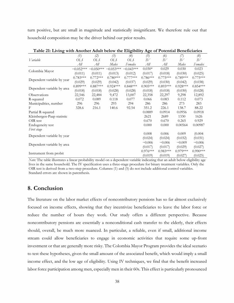
38

turn positive, but are small in magnitude and statistically insignificant. We therefore rule out that

household composition may be the driver behind our prior results.

Table 21: Living with Another Adult below the Eligibility Age of Potential Beneficiaries

Variable (1) (2) (3) (4) (5) (6) (7) (8)

OLS OLS OLS OLS IV IV IV IV All All Males Females All All Males Females

Colombia Mayor −0.052*** −0.050*** −0.053*** −0.043*** 0.030* 0.029 0.030 0.023 (0.011) (0.011) (0.013) (0.012) (0.017) (0.018) (0.030) (0.025)

Dependent variable by year 0.783*** 0.772*** 0.780*** 0.777*** 0.786*** 0.775*** 0.789*** 0.775*** (0.029) (0.029) (0.042) (0.037) (0.029) (0.030) (0.042) (0.038)

Dependent variable by area 0.899*** 0.887*** 0.924*** 0.848*** 0.905*** 0.893*** 0.928*** 0.854*** (0.018) (0.018) (0.028) (0.028) (0.018) (0.018) (0.030) (0.028)

Observations 22,546 22,484 9,472 13,007 22,358 22,297 9,298 12,892 R-squared 0.072 0.089 0.118 0.077 0.066 0.083 0.112 0.073 Municipalities, number 296 296 293 294 286 286 273 283 F 328.6 216.1 140.6 92.54 351.2 226.1 138.7 88.22 Partial R-squared 0.0889 0.0914 0.0956 0.0918 Kleinbergen-Paap statistic 2621 2689 1330 1626 OIR test 0.670 0.670 0.265 0.929 Endogeneity test 0.000 0.000 0.00564 0.00987 First stage

Dependent variable by year 0.008 0.006 0.009 (0.004 (0.024) (0.024) (0.032) (0.031)

Dependent variable by area −0.006 −0.006 −0.009 −0.006 (0.017) (0.017) (0.029) (0.027)

Instrument from probit 0.976*** 0.983*** 0.979*** 0.990*** (0.019) (0.019) (0.027) (0.025)

Note: The table illustrates a linear probability model on a dependent variable indicating that an adult below eligibility age lives in the same household. The IV specification uses a three-stage procedure for binary treatment variables. Only the OIR test is derived from a two-step procedure. Columns (1) and (5) do not include additional control variables. Standard errors are shown in parenthesis.

8. Conclusion The literature on the labor market effects of noncontributory pensions has so far almost exclusively

focused on income effects, showing that they incentivize beneficiaries to leave the labor force or

reduce the number of hours they work. Our study offers a different perspective. Because

noncontributory pensions are essentially a nonconditional cash transfer to the elderly, their effects

should, overall, be much more nuanced. In particular, a reliable, even if small, additional income

stream could allow beneficiaries to engage in economic activities that require some up-front

investment or that are generally more risky. The Colombia Mayor Program provides the ideal scenario

to test these hypotheses, given the small amount of the associated benefit, which would imply a small

income effect, and the low age of eligibility. Using IV techniques, we find that the benefit increased

labor force participation among men, especially men in their 60s. This effect is particularly pronounced

39

in occupations that require working alone as independent workers or in the cultivation of agricultural

land over which the beneficiaries have tenure rights. These results support the idea that liquidity

constraints prevented some beneficiaries from engaging in these economic activities. However, we

could not find any evidence for a shift from less risky to more risky activities. Moreover, we could

find no such results among women. Among men age 70 or older, some of these results persist, albeit

at a much lower magnitude.

Our findings have two important implications. First, they indicate that studies demonstrating support

for the negative aggregate effect of noncontributory pensions on beneficiary labor force participation

may confound two separate effects. Second, they add another outcome to the still understudied area

of the potential of cash transfer programs to ease liquidity constraints and increase economic activity.

The last point warrants more attention than it has thus far received.

40

References Adams, Renée, Heitor Almeida, and Daniel Ferreira. 2009. “Understanding the Relationship

between Founder-CEOs and Firm Performance.” Journal of Empirical Finance 16 (1): 136–50. Aguila, Emma, Arie Kapteyn, Rosalba Robles, and Beverly Weidmer. 2012. “Experimental Analysis

of the Health and Well-Being Effects of a Non-Contributory Social Security Program.” Rand Corporation, Santa Monica, CA.

Amarante, Verónica, Marco Manacorda, Andrea Vigorito, and Mariana Zerpa. 2011. “Social Assistance and Labor Market Outcomes: Evidence from the Uruguayan PANES.” Working paper, Inter-American Development Bank, Washington, DC.

Amuedo‐Dorantes, Catalina, and Laura Juarez. 2015. “Old‐Age Government Transfers and the Crowding Out of Private Gifts: The 70 and Above Program for the Rural Elderly in Mexico.” Southern Economic Journal 81 (3): 782–802.

Aterido, Reyes, Mary Hallward-Driemeier, and Carmen Pagés. 2011. “Does Expanding Health Insurance beyond Formal-Sector Workers Encourage Informality? Measuring the Impact of Mexico's Seguro Popular.” Policy Research Working Paper 5785, World Bank, Washington, DC.

Azuara, Oliver, and Ioana Marinescu. 2013. “Informality and the Expansion of Social Protection Programs: Evidence from Mexico.” Journal of Health Economics 32 (5): 938–50.

Barrientos, Armando. 2003. “What Is the Impact of Non-Contributory Pensions on Poverty? Estimates from Brazil and South Africa.” Development Economics and Public Policy Working Paper 30556, Institute for Development Policy and Management, University of Manchester, Manchester, U.K.

———. 2005. “Non-contributory Pensions and Poverty Reduction in Brazil and South Africa.” Working paper, Institute for Development Policy and Management, University of Manchester, Manchester, U.K.

Barrientos, Armando, and Peter Lloyd-Sherlock. 2003. “Non-contributory Pensions and Social Protection.” Issues in Social Protection Discussion Paper 12, International Labour Organization, Geneva.

Berg, Erlend. 2013. “Are Poor People Credit-Constrained or Myopic? Evidence from a South African Panel.” Journal of Development Economics 101 (March): 195–205.

Bosch, Mariano, and Raymundo M. Campos-Vázquez. 2010. “The Trade-Offs of Social Assistance Programs in the Labor Market: The Case of the ‘Seguro Popular’ Program in Mexico.” Documento de Trabajo 12–2010, Centro de Estudios Económicos, El Colegio de México, Mexico City.

Bosch, Mariano, and Jarret Guajardo. 2012. “Labor Market Impacts of Non-Contributory Pensions: The Case of Argentina's Moratorium.” IDB Working Paper 366, Inter-American Development Bank, Washington, DC.

Bosch, Mariano, Ángel Melguizo, and Carmen Pagés. 2013. Better Pensions, Better Jobs: Towards Universal Coverage in Latin America and the Caribbean. Washington, DC: Inter-American Development Bank.

Calderón-Mejía, Valentina, and Ioana Elena Marinescu. 2012. “The Impact of Colombia's Pension and Health Insurance Systems on Informality.” IZA Discussion Papers 6439, Institute for the Study of Labor, Bonn.

Camacho, Adriana, and Emily Conover. 2011. “Manipulation of Social Program Eligibility.” American Economic Journal: Economic Policy 3 (2): 41–65.

41

Camacho, Adriana, Emily Conover, and Alejandro Hoyos. 2014. “Effects of Colombia's Social Protection System on Workers’ Choice between Formal and Informal Employment.” World Bank Economic Review 28 (3): 446–66.

Colombia, Ministerio de Trabajo. 2013. Informe de Actividades 2012–2013 al Honorable Congreso de la República. July. Bogotá, Colombia: Ministerio de Trabajo.

———. 2014. Informe de Actividades 2013–2014 al Honorable Congreso de la República. July. Bogotá, Colombia: Ministerio de Trabajo.Duflo, Esther. 2003. “Grandmothers and Granddaughters: Old‐Age Pensions and Intrahousehold Allocation in South Africa.” World Bank Economic Review 17 (1): 1–25.

Duval-Hernández, Robert, and Ricardo Smith Ramírez. 2011. “Informality and Seguro Popular under Segmented Labor Markets.” Working paper, Centro de Investigación y Docencia Económicas, Mexico City.

Emery, J. C., and Jesse A. Matheson. 2012. “Should Income Transfers be Targeted or Universal? Insights from Public Pension Influences on Elderly Mortality in Canada, 1921–1966.” Canadian Journal of Economics 45 (1): 247–69.

Fogel, Nathan M. and Paes de Barros, Ricardo. 2010. “The Effect of Conditional Cash Transfer Programmes on Adult Labor Supply: An Empirical Analysis Using a Time-Series-Cross-Section Sample of Brazilian Municipalities.” Estudos Econômicos (São Paulo), 40(2), pages 259-293.

Galasso, Emanuela. 2006. “`With Their Effort and One Opportunity’: Alleviating Extreme Poverty in Chile.” Unpublished Working Paper.

Galiani, Sebastián, Paul Gertler, and Rosangela Bando. 2014. “Non-contributory Pensions.” IDB Working Paper 517, Inter-American Development Bank, Washington, DC.

Gasparini, Leonardo, and Nora Lustig. 2011. “The Rise and Fall of Income Inequality in Latin America.” ECINEQ Working Paper 213, Society for the Study of Economic Inequality, Dipartimento de Scienze Economiche, Università di Verona, Verona, Italy.

Gertler, Paul J., Sebastian Martinez, and Marta Rubio-Codina. 2006. “Investing Cash Transfers to Raise Long Term Living Standards.” Policy Research Working Paper 3994, World Bank, Washington, DC.

Haushofer, Johannes, and Jeremy Shapiro. 2013. “Household Response to Income Changes: Evidence from an Unconditional Cash Transfer Program in Kenya.” Working paper, Massachusetts Institute of Technology, Cambridge, MA.

Johnson, Jessica K. M., and John B. Williamson. 2006. “Do Universal Non-Contributory Old-Age Pensions Make Sense for Rural Areas in Low-Income Countries?” International Social Security Review 59 (4): 47–65.

Juárez, Laura. 2009. “Crowding Out of Private Support to the Elderly: Evidence from a Demogrant in Mexico.” Journal of Public Economics 93 (3): 454–63.

———. 2010. “The Effect of an Old-Age Demogrant on the Labor Supply and Time Use of the Elderly and Non-Elderly in Mexico.” B. E. Journal of Economic Analysis & Policy 10 (1): 1–27.

Juárez, Laura, and Tobias Pfutze. 2015. “The Effects of a Non-Contributory Pension Program on Labor Force Participation: The Case of 70 y Más in Mexico.” Economic Development and Cultural Change 63 (4): 685–713.

Knox, Melissa A., and Raymundo M. Campos-Vázquez. 2010. “Social Protection Programs and Employment: The Case of Mexico’s Seguro Popular Program.” Documento de Trabajo 14–2010, Centro de Estudios Económicos, El Colegio de México, Mexico City.

Lustig, Nora, and Carola Pessino. 2014. “Social Spending and Income Redistribution in Argentina during the 2000s: The Increasing Role of Noncontributory Pensions.” Public Finance Review 42 (3): 304–25.

42

Maluccio, John A. and Flores, Rafael. 2005. “Impact Evaluation of a Conditional Cash Transfer Program: The Nicaraguan Red de Protección Social.” International Food Policy Research Institute Research Report 141.

Martinez, Sebastian. 2004. “Pensions, Poverty, and Household Investments in Bolivia.” Doctoral dissertation, University of California at Berkeley, Berkeley, CA.

Miller, Grant, Diana Pinto, and Marcos Vera-Hernández. 2013. “Risk Protection, Service Use, and Health Outcomes under Colombia’s Health Insurance Program for the Poor.” American Economic Journal: Applied Economics 5 (4): 61–91.

Posel, Dorrit, James A. Fairburn, and Frances Lund. 2006. “Labour Migration and Households: A Reconsideration of the Effects of the Social Pension on Labour Supply in South Africa.” Economic Modelling 23 (5): 836–53.

Ribas, Rafael P. 2014. “Direct and Indirect Effects of Cash Transfers on Entrepreneurship.” Paper presented at the Agricultural and Applied Economics Association’s 2014 Annual Meeting, Minneapolis, July 27–29.

Rofman, Rafael, Ignacio Apella, and Evelyn Vezza, eds. 2015. Beyond Contributory Pensions: Fourteen Experiences with Coverage Expansion in Latin America. Report 92872. Directions in Development: Human Development. Washington, DC: World Bank.

Rubio, Jose. 2014. “The Effect of Non-contributory Pensions on the Health and Welfare of the Elderly Poor in Colombia.” Master’s Dissertation SA4A6, London School of Economics and Political Science, London.

Rubio, Jose, Phillip Hessel, and Mauricio Avendano. 2015. “Do Income Transfers for the Old Improve Health? The Impact of a Non-contributory Pension Programme on Old-Age Health in Colombia.” Paper presented at the Population Association of America’s 2015 Annual Meeting, San Diego, April 30–May 2.

Salinas-Rodríguez, Aarón, Ma Del Pilar Torres-Pereda, Betty Manrique-Espinoza, Karla Moreno-Tamayo, and Martha María Téllez-Rojo Solís. 2014. “Impact of the Non-Contributory Social Pension Program 70 y más on Older Adults’ Mental Well-Being.” PLoS One 9 (11): 1–10.

Shea, John. 1997. “Instrument Relevance in Multivariate Linear Models: A Simple Measure.” Review of Economics and Statistics 79 (2): 348–52.

Skoufias, Emmanuel and di Maro, Vincenzo. 2006. “Conditional Cash Transfers, Adult Work Incentives, and Poverty.” World Bank Policy Research Working Paper 3973.

Skoufias, Emmanuel, Mishel Unar, and Teresa Gonzalez de Cossio.2013. “The Poverty Impacts of Cash and In-Kind Transfers: Experimental Evidence from Rural Mexico.” Journal of Development Effectiveness. DOI: 10.1080/19439342.2013.843578

Soares, Fábio Veras, Rafael Perez Ribas, and Rafael Guerreiro Osório. 2010. “Evaluating the Impact of Brazil's Bolsa Família: Cash Transfer Programs in Comparative Perspective.” Latin American Research Review 45 (2): 173–90.

Stock, James H., Jonathan Wright, and Motohiro Yogo. 2002. “A Survey of Weak Instruments and Weak Identification in Generalized Method of Moments.” Journal of Business and Economic Statistics 20 (4): 518–29.

Wooldridge, Jeffrey M. 2010. Econometric Analysis of Cross Section and Panel Data. 2nd ed. Cambridge, MA: MIT Press.