can analysts detect earnings management: evidence from ... · adjust their cash flow forecasts...

Can Analysts Detect Earnings Management:

Evidence from Firm Valuation

By

Lucie Courteaua

Jennifer L. Kaob

and

Yao Tianc

July 2011 (Preliminary version, please do not quote without the authors’ permission)

a. School of Economics and Management, Free University of Bolzano, Bolzano, Italy, Tel: +39 0471 013130; Email: [email protected]

b. Department of AMIS, University of Alberta, Edmonton, Alberta, Canada, Tel: (780) 492-7972; Email:[email protected]

c. Department of AMIS, University of Alberta, Edmonton, Alberta, Canada, Tel: (780) 492-8008; Email:[email protected]

Acknowledgments. We would like to thank Gord Richardson, workshop participants at the University of Bocconi and participants at the Annual Conference of the European Accounting Association, in Rome, for their helpful comments on an earlier version of the paper. Financial support for this project is provided by the University of Alberta (SSHRC 4A and Canadian Utilities fellowship) and the Free University of Bolzano.

1

Can Analysts Detect Earnings Management: Evidence from Firm Valuation

Abstract: In this paper, we present empirical evidence on whether financial analysts can see through earnings management and whether their earnings and cash flow forecasts take into account the effect of accrual manipulations. Prior studies looking into analyst behaviour vis-à-vis earnings management have typically drawn inferences from the direction or magnitude of analyst earnings forecast errors. Interpreting low earnings forecast errors as absence of accrual manipulations is nonetheless problematic. As well, lower earnings forecast errors do not necessarily imply higher forecast quality.

We overcome these methodological difficulties by employing an alternative research design that focuses on the valuation usefulness of analyst earnings and cash flow forecasts, measured by the absolute value of percentage valuation errors under the RIM and DCF models, using three- or five-year ex-post intrinsic value as the benchmark. Large valuation errors imply that a model is less useful for valuation purposes. Regressing valuation errors on the extent of accrual manipulations (DACC), we find that the coefficient estimate on DACC is positive and significant in the RIM regression, but insignificantly different from zero in the DCF regression. Results continue to hold when we re-define valuation benchmark as stock price at the forecast date, implying that analysts can see through earnings management but choose to forecast managed earnings while adjusting cash flow forecasts to reflect earnings management. Taken together, these results suggest that analysts issue earnings forecasts strategically and that large valuation errors do not reflect analysts’ inability to detect and incorporate the consequences of earnings management in their earnings forecasts.

JEL Classification: M41

Key Words: Analyst Forecasts; Earnings Management; Valuation Errors

2

1. Introduction

Earnings are used extensively to evaluate firm performance and estimate firm value. The

majority of the 400 CFOs surveyed by Graham, Harvey and Rajgopal (2005) believe that

earnings, not cash flows, are the key metric used by outside stakeholders. However, evidence

suggests that earnings are often subject to managerial manipulations. Such manipulations,

driven by the pressure to meet or beat earnings expectations, are believed to have eroded the

quality of earnings and led to highly publicized corporate scandals such as Enron and

WorldCom in the early 2000s. The perceived erosion of financial reporting quality in turn

prompted the US Congress to pass the Sarbanes-Oxley Act (SOX) on July 30, 2002 with the

stated objective of restoring investor confidence in financial and public reporting. The role

earnings management plays in the capital market depends on whether at least some of the

market participants can detect such practice. Research has shown that the accrual component

of earnings is not as persistent as the cash flow component of earnings (Sloan 1996) and that

the lack of persistence is driven mainly by the discretionary component of the accruals (Xie

2001). However, investors do not seem to recognize the difference in the persistence of

different income components – they overreact to the accrual component of earnings and

underreact to the cash flow component.

The purpose of this study is to examine whether sophisticated market participants,

such as financial analysts, can detect accrual manipulations and if so whether they take into

consideration accrual manipulations in their forecasts. Evidence from prior research in this

area is mixed (Givoly, Hayn and Yoder 2008). On one hand, several studies have shown that

firms with unusually large accruals have large negative earnings forecast errors, defined as

the difference between realized earnings and forecasted earnings (Abarbanell and Lehavy

2003; Bradshaw, Richardson and Sloan 2001). Ahmed, Nainar and Zhou (2005) also find that

analysts give discretionary accruals the same weight as non-discretionary accruals when

3

forecasting future earnings, even though the former is less persistent. Finally, Hribar and

Jenkins (2004) report that analysts do not anticipate the consequence of earnings management

that leads to restatements later on. Collectively, results from these studies suggest that

analysts cannot detect earnings management, or at least do not fully account for its effect on

firm future performance in their forecasts. Other researchers however show that analysts can

detect and account for accrual manipulations. Burgstahler and Eames (2003) for example find

that analysts have some ability to identify firms that may have engaged in earnings

management to avoid small earnings declines. Liu (2004) also reports that analyst forecasts

are on average below (above) the level obtained when strategic incentives are not at play for

firms with negatively (positively) skewed earnings. The observed patterns of analyst forecasts

reported in these two studies support the notion that financial analysts are able to anticipate

the prospect of accrual manipulations and that they take into account that expectation in their

forecasts to avoid large optimistic or large pessimistic forecast errors.

The aforementioned studies draw inferences about how analysts deal with accrual

manipulations from the direction or magnitude of analyst earnings forecast errors. However,

since earnings forecast errors can be artificially reduced if analysts choose to forecast

managed earnings, looking at analyst earnings forecast errors alone cannot tell us whether

analysts can detect accrual manipulations and choose to forecast managed earnings, or they

cannot detect accrual manipulations and simply follow management's earnings guidance to

achieve higher forecast accuracy. Further complications arise from uncertainty about whether

financial analysts forecast managed or unmanaged earnings in practice given their economic

incentives and reputation concerns. Burgstahler and Eames (2003) show that the distribution

of analyst earnings forecasts has a ‘kink’ around zero, much like that for the distribution of

earnings documented in Dechow, Richardson and Tuna (2003), implying that analysts

forecast managed earnings. Evidence from the expectations management literature suggests a

4

complex interplay between managers and financial analysts. To meet or beat analyst

forecasts, managers have a strong incentive to guide the forecasts downward from the

beginning to the end of the year (Richardson, Teoh and Wysocki 2004; Bartov, Givoly and

Hayn 2002). From analysts’ perspective, it may be rational to issue optimistic earnings

forecasts even if they are aware of the manager’s incentive to manage earnings, as such

forecasts will yield smaller forecast errors (Beyer 2008). Another problem with looking at

analyst forecast errors is that lower earnings forecast errors do not necessarily imply higher

forecast quality. O’Brien (1988) argues that forecast quality should ultimately depend on the

context in which forecasts are used.

In light of the difficulties in inferring analyst behaviour vis-à-vis earnings

management from analyst earnings forecast errors, we employ a different research design that

focuses on the valuation usefulness of analyst earnings and cash flow forecasts in this study.

We define valuation usefulness as the valuation errors between firm value computed from the

residual income (RIM) or discounted cash flows (DCF) model that uses earnings or cash flow

forecasts as inputs and ex-post measure of intrinsic firm value (calculated as the sum of actual

dividends over a three-year (or five-year) horizon and market price at the horizon, discounted

at the industry cost of equity (Subramanyam and Venkatachalam 2007)). Following O’Brien

(1988), we view forecast quality as the ability of analyst forecasts to incorporate information,

such as accrual manipulations, that is relevant for firm valuation.

Our research design calls for comparing the valuation usefulness of analyst earnings

(or cash flow) forecasts in a setting where there is earnings management versus where there is

not. We consider the following three scenarios: First, analysts can see through earnings

management, but choose to forecast managed earnings in order to minimize earnings forecast

errors. In this case, analysts would apply their knowledge about earnings management to

5

adjust their cash flow forecasts because they also want to minimize cash flow forecast errors.1

Thus, using earnings forecasts in firm valuation based on RIM will yield relatively larger

valuation errors for accrual manipulators, whereas using cash flow forecasts based on DCF

will result in similar valuation errors with or without the presence of reporting bias. Second,

analysts can see through earnings management and choose to forecast pre-managed earnings

even though doing so will produce larger earnings forecast errors. In this scenario, earnings

management is not expected to affect valuation errors for either RIM or DCF model, as both

earnings and cash flow forecasts are based on the persistent part of reported earnings. Third,

analysts cannot see through earnings management and use reported earnings as a basis for

their earnings and cash flow forecasts. For accrual manipulators, part of the current earnings

that serve as a basis for forecasts is managed and hence is purely transitory. Yet analysts

incorporate the transitory component as if it were persistent, resulting in higher valuation

errors under both RIM and DCF, compared to the case when there is no earnings

management.

To carry out the analysis, we use earnings and cash flow forecasts provided by Value

Line (VL) analysts because VL provides both types of forecasts for all firms that it follows.

Moreover, VL analysts are in-house and, unlike analysts contributing forecasts to IBES, they

are not subject to investment banking relations, thus limiting VL analysts’ incentives to play

the earnings management game in cooperation with management (Brav, Lehavy and

Michaely 2005). Our sample is drawn from an eleven-year (1990–2000) period that pre-dates

major corporate scandals and the ensuing legislative events, allowing us to better isolate the

effect of earnings management on the earnings and cash flow forecasts. In our main analysis,

the final sample consists of 4,586 firm-year observations with complete annual

financial/stock price information and forecast data. We measure the extent of accrual 1 Call, Chen and Tong (2009) for example show that more accurate cash flow forecasts can yield favourable career outcomes for analysts and reduce the likelihood of their being fired.

6

management by the absolute value of the discretionary accruals estimated from a version of

the Dechow et al.’s (2003) forward-looking modified Jones model (FLMJ).

Results indicate that the ability of the RIM model to predict firm value is diminished

by the presence of earnings management, whereas the valuation usefulness of the DCF model

remains unchanged. These results are consistent with the predictions of the first scenario,

referred to above. That is, analysts can see through earnings management, but choose to

forecast managed earnings while at the same time take earnings management into

consideration in their cash flow forecasts. This behaviour suggests that analyst earnings

forecasts are strategic in nature and that large valuation errors associated with using such

forecasts as inputs in the RIM model do not reflect analysts’ inability to detect, and

incorporate the consequences of, earnings management in their earnings forecasts.

Our study sheds light on the role played by financial analysts in interpreting and

disseminating financial information. We present evidence that analysts’ ability to detect

earnings management and incorporate such information into their forecasts can directly affect

firm valuation when there is reporting bias. We also contribute to the valuation literature,

which has traditionally used analyst forecasts as part of the inputs for firm valuation. While

including analyst forecasts in valuation models has been shown to improve the ability of

these models to predict firm value (Lee, Myers and Swaminathan 1999; Frankel and Lee

1998), we show that the valuation usefulness of analyst earnings forecasts may be greatly

diminished during a time when a non-trivial number of firms are believed to have engaged in

earnings management practice. Finally, our study is of practical relevance. Earnings are used

extensively to evaluate firm performance and estimate firm value in practice (Skinner and

Sloan 2002). However, when earnings are managed, heavy reliance on this number in firm

valuation may result in inaccurate assessment, undesirable investment decisions and

misallocation of resources. We quantify this effect and raise awareness among investors and

7

practitioners about the pitfalls of taking managed earnings at face value and using them

directly in firm valuation.

The remainder of the paper is organized as follows: Section 2 reviews the relevant

literature and develops the hypotheses; Section 3 discusses the research methodology, along

with variable definitions and measurements; Section 4 summarizes our sample selection

procedure; Section 5 presents the main empirical findings; and Section 6 concludes the study.

2. Literature Review

Earnings Management

Healy and Wahlen (1999) remark that “... earnings management occurs when managers use

judgment in financial reporting and structuring transactions to alter financial reports to either

mislead some stakeholders about the underlying economic performance of the company or to

influence contractual outcomes that depend on reported accounting numbers.” Studies have

shown that firms often manage their earnings in advance of IPOs and seasoned equity

offerings (Erickson and Wang 1999; Teoh, Welch and Wong 1998a; Teoh, Welch and Wong

1998b; Dechow, Sloan and Sweeney 1996) and that firms involved in earnings manipulations

or singled out by the SEC for accounting enforcement actions generally have weak internal

governance (Farber 2005; Bédard, Marrakchi-Chtourou and Courteau 2004; Klein 2002;

Beasley 1996; Dechow et al. 1996).

Several factors have been cited as contributing to a firm’s motivation to meet or beat

earnings targets by managing reported earnings. First, the stock market tends to punish firms

for falling short of earnings expectations (Skinner and Sloan 2002). In particular, firms

maintaining strings of steadily increasing earnings are rewarded with market premiums and

are severely punished as soon as the strings are broken (Myers, Myers and Skinner 2006;

8

Barth, Elliott and Finn 1999). Second, meeting or beating earnings targets allows executives

to enhance their reputation with stakeholders, enjoy better terms of trade and achieve higher

bonus compensations (DeGeorge, Patel and Zeckhauser 1999; Burgstahler and Dichev 1997;

Bowen, DuCharme and Shores 1995; Healy 1985). Failing to meet earnings expectations

could result in reputation loss and pay cuts for CEOs (Matsunaga and Park 2001).

Countering these incentives to meet or beat earnings targets are the capital market

consequences that firms face when their alleged earnings manipulations become public

(Dechow et al. 1996). If the market is efficient, then its participants should be able to spot

earnings management practices and undo manipulations to reflect real economic earnings for

use in firm valuation. However, corporate disclosures often do not contain sufficient

information for the investors to infer accounting accruals, limiting their ability to account for

earnings management (Gleason and Mills 2008; Baber, Chen and Kang 2006; Balsam, Bartov

and Marquardt 2002).

Analysts’ Reaction to Earnings Management

Empirical evidence on whether sophisticated users of accounting information, such as

financial analysts, cansee through earnings management and include its future effects in their

forecasts is mixed. Bradshaw, Richardson and Sloan (2001) for example find large negative

earnings forecast errors (optimism) for firms with unusually large accruals. Abarbanell and

Lehavy (2003) report a similar association between analyst optimism and three types of

accruals: large income-decreasing accruals used in a loss year to accumulate reserves for

future years; small income-decreasing accruals to bring the earnings down to the target level

in profitable years and replenish accrual reserves; income-increasing accruals to meet or just

beat earnings targets. Regressing earnings and earnings forecasts on previous year’s earnings

components, Ahmed, Nainar and Zhou (2005) show that discretionary accruals are given the

9

same weight as non-discretionary accruals by analysts in forecasting future earnings even

though they are less persistent. Finally, for 259 of their 292 restatement observations Hribar

and Jenkins (2004) find that at least one analyst revised his earnings forecasts downwards

following restatements and that the average revisions were -14.7% for the one-year ahead

forecasts and -7.8% for two years ahead. Taken together, the results of these studies are

consistent with the notion that analysts cannot detect earnings management or fully reflect its

implications for future performance in their forecasts.

However, it is possible that analysts can see through earnings management, but for

strategic reasons choose to forecast managed rather than pre-managed earnings. The strategic

incentives arise because most analysts are rewarded, financially or reputationally, for their

ability to issue accurate earnings forecasts (Hong and Kubik 2003; Mikhail, Walther and

Willis 1997). Thus, analysts may be motivated to minimize forecast errors by strategically

adjusting their earnings forecasts upwards or downwards to fit the managed, rather than the

pre-managed, earnings. Evidence from the expectations management literature supports this

view. According to Richardson et al. (2004) and Bartov et al. (2002), analysts cooperate with

management in the earnings game by issuing optimistic forecasts at the beginning of the year

to demonstrate their confidence in the firm. This is then followed by downward forecast

revisions during the year at the management’s guidance, allowing the firm to meet or beat

earnings expectation and the analysts to lower their forecast errors at the end of the year - a

win-win situation for both parties.

10

3. Research Methodology

Accrual Management

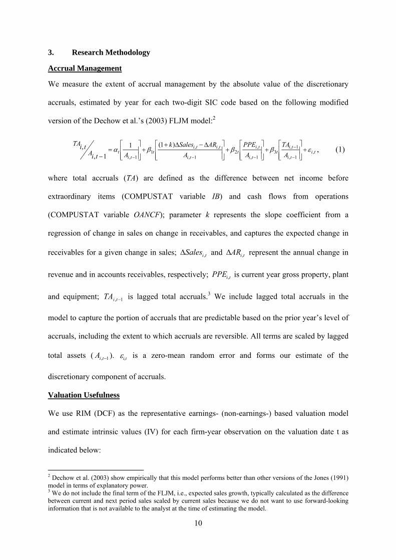
We measure the extent of accrual management by the absolute value of the discretionary

accruals, estimated by year for each two-digit SIC code based on the following modified

version of the Dechow et al.’s (2003) FLJM model:2

ti

ti

tit

ti

tit

ti

titit

tit A

TA

A

PPE

A

ARSalesk

AtiAtiTA

,1,

1,3

1,

,2

1,

,,1

1,

)1(1

1,

,

, (1)

where total accruals (TA) are defined as the difference between net income before

extraordinary items (COMPUSTAT variable IB) and cash flows from operations

(COMPUSTAT variable OANCF); parameter k represents the slope coefficient from a

regression of change in sales on change in receivables, and captures the expected change in

receivables for a given change in sales; tiSales , and tiAR , represent the annual change in

revenue and in accounts receivables, respectively; tiPPE , is current year gross property, plant

and equipment; 1, tiTA is lagged total accruals.3 We include lagged total accruals in the

model to capture the portion of accruals that are predictable based on the prior year’s level of

accruals, including the extent to which accruals are reversible. All terms are scaled by lagged

total assets ( 1, tiA ). i,t is a zero-mean random error and forms our estimate of the

discretionary component of accruals.

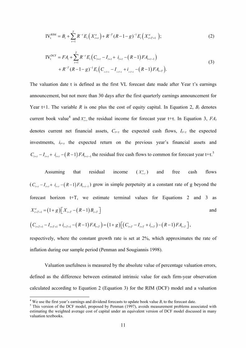
Valuation Usefulness

We use RIM (DCF) as the representative earnings- (non-earnings-) based valuation model

and estimate intrinsic values (IV) for each firm-year observation on the valuation date t as

indicated below:

2 Dechow et al. (2003) show empirically that this model performs better than other versions of the Jones (1991) model in terms of explanatory power. 3 We do not include the final term of the FLJM, i.e., expected sales growth, typically calculated as the difference between current and next period sales scaled by current sales because we do not want to use forward-looking information that is not available to the analyst at the time of estimating the model.

11

RIM 1t 1

1

IV ( 1 ) ;T

a T at t t t t TB R E X R R g E X

(2)

1 1 1

DCFt 1

1

1

IV 1

( 1 ) 1 .t T t T t T

T

t t t t t t

Tt t T

FA R E C I i R FA

R R g E C I i R FA

(3)

The valuation date t is defined as the first VL forecast date made after Year t’s earnings

announcement, but not more than 30 days after the first quarterly earnings announcement for

Year t+1. The variable R is one plus the cost of equity capital. In Equation 2, Bt denotes

current book value4 and atX the residual income for forecast year t+τ. In Equation 3, FAt

denotes current net financial assets, Ct+τ the expected cash flows, It+τ the expected

investments, it+τ the expected return on the previous year’s financial assets and

11t t t tC I i R FA the residual free cash flows to common for forecast year t+τ.5

Assuming that residual income ( atX ) and free cash flows

( 11t t t tC I i R FA ) grow in simple perpetuity at a constant rate of g beyond the

forecast horizon t+T, we estimate terminal values for Equations 2 and 3 as

1 1 1at T t T t TX g X R B and

1 1 1 1 1 1t T t T t T t T t T t T t T t TC I i R FA g C I i R FA ,

respectively, where the constant growth rate is set at 2%, which approximates the rate of

inflation during our sample period (Penman and Sougiannis 1998).

Valuation usefulness is measured by the absolute value of percentage valuation errors,

defined as the difference between estimated intrinsic value for each firm-year observation

calculated according to Equation 2 (Equation 3) for the RIM (DCF) model and a valuation

4 We use the first year’s earnings and dividend forecasts to update book value Bt to the forecast date. 5 This version of the DCF model, proposed by Penman (1997), avoids measurement problems associated with estimating the weighted average cost of capital under an equivalent version of DCF model discussed in many valuation textbooks.

12

benchmark, scaled by the latter. Larger absolute percentage valuation errors imply that a

model is less useful for valuation purposes. We use ex post intrinsic value (IV) as the

valuation benchmark, calculated as the sum of actual dividends over a three-year (or five-

year) horizon and market price at the horizon, discounted at the industry cost of equity

(Subramanyam and Venkatachalam 2007).6

Research Model

We use the following multivariate regression models:

AE_RIM = a0 + a1DACC+ a2BM + a3ES + a4Std_ROE + ε1, (4)

AE_DCF = b0 + b1DACC + b2BM + b3ES + b4Std_ROE + ε2, (5)

where the dependent variable AE_RIM (AE_DCF) denotes the absolute percentage valuation

errors for each firm-year observation under RIM (DCF); DACC is the test variable given by

the absolute value of the residuals from Equation 1. Equations 4 and 5 also include three

control variables found to affect the predictability of earnings in prior literature:7 (1) Book-to-

Market ratio (BM), defined as book value per share over stock price, measured at the end of

Year t; (2) Earnings shock (ES), defined as the absolute value of the change in net income

from Year t–1 to Year t, scaled by opening total assets; (3) Standard deviation of return on

equity (Std_ROE) over a 5-year period immediately preceding the end of Year t.

The estimated coefficient a1 (b1) captures the impact of accrual manipulations on the

valuation usefulness of analyst earnings (cash flow) forecasts in firm valuation based on the

RIM (DCF) model. A positive and significant a1 (b1) implies that the RIM (DCF) model is

less useful for firm valuation in the presence of reporting bias. On the other hand, if the

6 The ex-post intrinsic value is based on stock prices at the end of three-year horizon, as studies have found that the anomalous pricing of accruals and cash flows does not persist beyond two years (Xie 2001; Sloan 1996). 7 See Lang and Lundholm (1996), Kross, Ro and Schroeder (1990) and Brown, Richardson and Schwager (1987).

13

coefficient estimate on the test variable DACC (i.e., a1 or b1) is insignificantly different from

zero, then the valuation usefulness is said to be unaffected by accrual manipulations for the

model in question.

Predictions

Our interest in this study is to investigate the ability of financial analysts to detect accrual

manipulations and whether they incorporate such information into their earnings and cash

flow forecasts. To address these two research questions, we consider the following three

scenarios: (1). Analysts can see through earnings management, but choose to forecast

managed earnings in order to minimize earnings forecast errors. (2). Analysts can see through

earnings management and choose to forecast pre-managed earnings. (3). Analysts cannot see

through earnings management and use managed earnings to construct their earnings and cash

flow forecasts.

Under Scenario 1, we expect the valuation usefulness of the RIM model to be lower

for accrual manipulators, i.e., firms with higher discretionary accruals. Since the incentive to

minimize forecast errors likely extends to cash flow forecasts, analysts will try to correct such

forecasts in order to eliminate the effect of earnings management, resulting in no difference

in the valuation usefulness of the DCF model for accrual manipulators and non-manipulators.

Evidence that a1 is positive and significant in Equation 4, whereas b1 is insignificantly

different from zero in Equation 5, is consistent with Scenario 1. In Scenario 2, we expect both

RIM and DCF models to have similar valuation usefulness for firms with high vs. those with

low discretionary accruals, as analysts consistently base their forecasts on the persistent part

of reported earnings. Thus, both a1 and b1 are predicted to be insignificantly different from

zero. Finally, under Scenario 3 the valuation usefulness of both RIM and DCF models is

expected to be lower for firms with high discretionary accruals than for firms with low

14

discretionary accruals. This is because analyst earnings and cash flows forecasts are both

based on managed earnings which are partly transitory in nature. In this case, both a1 and b1

are predicted to be positive and significant.

To address the question of whether financial analysts can detect accrual

manipulations, we focus on the contrasting predictions on b1 under Scenarios 1 and 3. The

notion that analysts can (cannot) see through accrual manipulations is consistent with a

positive and significant coefficient estimate on a1 and an insignificant (positive and

significant) coefficient estimate on b1. To address the question of whether financial analysts

incorporate their knowledge of accrual manipulations into forecasts, we compare the

contrasting predictions on a1 under Scenarios 1 and 2. The notion that analysts remove (do

not remove) the effects of accrual manipulations from their forecasts is consistent with an

insignificant (positive and significant) coefficient estimate on a1 and an insignificant

coefficient estimate on b1.

We do not offer directional predictions for any of the control variables. While

unpredictable earnings due to high growth, large earnings shocks and highly volatile past

returns can reduce RIM’s ability to estimate a firm’s intrinsic value, analyst forecasts of

future cash flows may not be completely independent of these factors.

4. Sample Selection

Our initial sample consists of 39,826 annual earnings announcements made between January

1, 1990 and December 31, 2000 by publicly traded US firms with complete financial and

stock price information on COMPUSTAT and CRSP, respectively, during the announcement

year. Following the convention of prior literature, we exclude observations in the Financial

(SIC codes 6022–6200) and Insurance (SIC codes 6312–6400) industries because they use

15

special accounting rules, making them unsuitable for comparison with firms in other

industries.

We then apply the following four filters to the initial sample: (1) Forecasted valuation

attributes are available from the Datafile and Historical Reports published by Value Line

Investor Services.8 (2) Financial data and stock price information required to compute the ex

post intrinsic value over a three-year (or five-year) period following the fiscal year-end, are

available from COMPUSTAT and CRSP, respectively. (3) Data required to construct all

regression variables are available. (4) Observations in the top and bottom 1% of the

distribution for each input into the valuation models and each independent variable in

Equations 4-5 are considered extreme and hence are deleted from the analysis.9 The above

filters reduce the initial sample by 33,233, 1,409, 68 and 530 firm-year observations,

respectively, resulting in a final sample of 4,586 firm-year observations summarized in Panel

A of Table 1.

Panel B of Table 1 presents the distribution of our sample by year. With the exception

of 1990, the observations are fairly evenly distributed over the eleven-year (1990-2000)

sample period, ranging from a low 7.52% in 2000 to a high of 10.68% in 1994. As is evident

in Panel C of Table 1, the industry distribution shows quite an even representation across

most sectors, as defined in Fama and French (1993), except for the Utilities industry which

accounts for 12.54% of the firms included in the sample. This is a reflection of the

deregulation of the energy sector in the 1990s.

8 We choose not to use IBES forecast data in this study because, compared to VL, IBES provides a more limited range of forecasted valuation attributes that excludes cash flow forecasts for a large proportion of the firms covered (Givoly, Hayn and Lehavy 2009). Moreover, unlike VL whose forecasts are provided by a single in-house analyst, analysts contributing to IBES generally have investment banking relationships with the firms they follow, potentially affecting their incentives to issue unbiased forecasts. Finally, recent studies find that analyst earnings forecasts are more accurate when accompanied by cash flow forecasts (Call et al. 2009) and target price forecasts (Gell, Homburg and Klettke 2010). VL analysts provide all three for all the firms that they follow.

9 All the regression results without trimming (not reported) are qualitatively similar.

16

[Insert Table 1 about Here]

5. Empirical Results

5.1 Descriptive Statistics

Panel A of Table 2 reports the descriptive statistics on all the model variables in Equations 4

and 5. The mean (median) market value of our sample firms is $3.13 billion ($1.13 billion).

While firms followed by Value Line are in general large, some smaller firms are also

included in the coverage, as evidenced in large standard deviation of market value (i.e., $8.73

billion). The mean absolute discretionary accruals represent 4% of total assets (DACC). The

overall mean (median) absolute percentage valuation errors are 0.412 (0.386) for the

earnings-based RIM model and 0.484 (0.427) for the non earnings-based DCF model. These

figures are also in line with those documented in the valuation literature. 10

Panel B of Table 2 presents pair-wise Pearson (Spearman) correlations among our

model variables in Equations 4 and 5, appearing above (below) the diagonal. The Pearson

correlation between the level of discretionary accruals (DACC) and AE_RIM is significantly

positive at the 1% level (0.070), whereas that between DACC and AE_DCF is insignificantly

different from zero. These pair-wise correlations offer preliminary evidence at the univariate

level that discretionary accruals adversely affect valuation usefulness of RIM, but not DCF

model (Scenario 1). Two of the control variables, ES and Std_ROE, have positive Pearson

correlations with AE_RIM (AE_DCF), i.e., 0.111 and 0.111 (0.029 and 0.092), significant at

the 5% level or better. The correlation between AE_DCF and the remaining control variable

BM is also significantly positive (0.055), while AE_RIM is negatively correlated with BM (-

0.065). The Spearman correlations show a similar pattern, except that the positive correlation

between AE_DCF and BM becomes negative but insignificant. These descriptive statistics 10 Courteau, Kao and Richardson (2001) for example report that over a five-year sample period (1992-1996) the mean absolute percentage pricing errors for their DCF and RIM models are 0.397 and 0.372, respectively.

17

point to the need to control for all three variables in the analysis of valuation accuracy of

RIM and DCF, as we do in a multivariate setting.11


5.2 Univariate Analysis

Table 3 presents the mean and median absolute valuation errors, compared across three

groups of firms based on their level of absolute discretionary accruals. Three-year (five-year)

absolute percentage valuation errors are based on ex-post intrinsic values computed from

dividends and stock prices over a period of three (five) years after the current fiscal year-end.

The three-year RIM valuation errors show a progressive increase between the low-DACC and

the high-DACC groups of firms, from 0.397 to 0.408 to 0.430, suggesting that the errors

increase with the level of earnings management. The difference in mean valuation errors

between the High and the Low DACC groups is significantly positive, at the 1% level (0.033,

t=3.26). The DCF valuation errors don’t seem to follow the same pattern, however. The mean

errors are 0.489, 0.475 and 0.488 for the Low, Medium and High groups, respectively.

Moreover, the small difference between the valuation errors of the High and the Low groups

is not statistically significant (-0.001, t=-0.11). Hence, the performance of the earnings-based

valuation model seems to be adversely affected by the level of earnings management, while

the cash flow-based model seems unaffected. Together, these results are consistent with

Scenario 1 described in Section 3: the VL analysts can see through earnings management and

use this knowledge to prepare their cash flow forecasts, but choose to forecast managed

rather than pre-managed earnings.

The second part of Panel A shows the results of the same tests using ex-post dividends

and stock prices over a five-year horizon as a benchmark for measuring valuation errors.12

11 The variance inflation factors of the regressions are all close to 1, indicating no serious problems of collinearity among the control variables.

18

While the RIM errors do not show the same progressive increase as for the three-year

benchmark, they are still significantly higher for the High-DACC than for the Low-DACC

firms (0.445 vs. 0.477, t=2.56). The difference in mean DCF errors is again non significant.

Hence, the five-year ex-post values yield results that are consistent with Scenario 1, although

the support is somewhat weaker than with the three-year horizon benchmark.

Panel B of Table 3 presents the comparison of median absolute valuation errors across

the three groups of firms. The non-parametric tests are used as a robustness check because of

the deviation of our sample’s distribution from normality. The results are as in Panel A: RIM

median absolute errors are significantly higher for firms with high DACC than for those of

the Low-DACC group, whereas the difference is not significant for the errors of the DCF

model.

Taken together, the results of the univariate analysis of absolute valuation errors are

consistent with the scenario where analysts can detect earnings management in the current

year and are aware of the fact that the bias in current earnings can affect the future

performance of the firm, but choose to forecast managed earnings, to maintain their record of

forecast accuracy.


5.3 Multivariate Analysis

The quality of analyst forecasts may be influenced by several factors other than earnings

management. In Table 4, we present the results of regression analyses that control for factors

which are likely to affect the association between valuation errors and earnings management.

As in the univariate analysis, we consider ex-post intrinsic values from both a three-year and

12 The sample size is reduced from 4,585 to 4,096 firm-year observations because of the attrition that occurs when requiring five years of dividends and prices, instead of three, to compute ex-post intrinsic values

19

a five-year horizon as benchmarks for computing valuation errors. The results are presented

in Panel A and Panel B, respectively.

The results in Panel A show that even when controlling for factors that may affect

earnings and cash flow predictability, the relationship between RIM valuation errors and

DACC is positive and significant at the 5% level (a1=0.263, t=2.35). When we move to the

AE_DCF regression, on the other hand, the coefficient on DACC is not significantly different

from zero (a1=0.075, t=0.51). These results are again consistent with Scenario 1. The control

variables are all significant in the RIM regression: The fact that the firm has an earnings

shock in the current year (ES), highly volatile performance (Std_ROE) or negative earnings

(Loss) all make it more difficult to predict its future performance, increasing the valuation

error. The variable BM, which is an inverse measure of firm growth, has a significantly

negative coefficient in the RIM regression, indicating that valuation errors are higher for

high-growth firms. In the DCF regression, the presence of an earnings shock in the current

period (ES) does not seem to affect the valuation error, while the coefficient on growth is

significantly positive. The adjusted R2 of the two regressions are quite low (0.025 and 0.014

for the RIM and the DCF models, respectively).

In Panel B, the five-year horizon valuation benchmark is used to compute the

dependent variables of the two regressions. In both models, the coefficient on DACC is

positive but not significantly different from zero (a1=0.202, t=1.47 for RIM and a1=0.039,

t=0.22 for DCF). Here, earnings management seems to affect neither the RIM nor the DCF

valuation errors. This is consistent with Scenario 2: the analysts see through earnings

management, but they choose to forecast pre-managed earning, using all the information

available to them to improve the quality of both their earnings and cash flow forecasts.

20

This result is surprising and raises the question as to why an analyst would choose to

act non-strategically and make earnings forecasts that he knows will not be accurate because

of the probable bias that managers will introduce in future earnings. This may be explained

by the fact that Value Line analysts may not be as sensitive to incentives related to forecast

accuracy as other analysts. In fact, Value Line does not provide any data on the ex-post

accuracy of its analysts’ forecast.


5.4 Pricing Errors

Until now, we have followed Subramanyam and Venkatachalam’s (2007) suggestion

to use ex-post intrinsic values as valuation benchmarks. The alternative, which has been used

extensively in the studies comparing the performance of valuation models, is to use the stock

price of the firm at the valuation date as a benchmark. This proxy is based on the assumption

that, at least on average, the market is efficient and that the market value of a firm is the best

estimate available of its intrinsic value.

Table 5 presents the results of the univariate (Panel A) and multivariate analyses

(Panel B) using current price as valuation benchmark. In Panel A, both mean and median

absolute errors show a progressive increase between the Low-DACC and the High-DACC

groups for RIM with a significant difference between the two extreme groups. The mean

absolute pricing errors are 0.296, 0.312 and 0.330 for the Low, Medium and High groups,

respectively, and the difference of 0.034 between High and Low is significantly different

from zero at the 1% level. The median errors show a similar pattern and a significant

difference in valuation performance between the groups of firms with the highest and the

lowest levels of discretionary accruals.

21

Panel B of Table 5 shows the results of the regression estimation of Equations (4) and

(5). The results are similar to those obtained with the three-year ex-post value benchmarks.

The coefficient on DACC is significantly positive for the RIM regression but not

significantly different from zero for the DCF regression. Hence, the results of Table 5 are

consistent with Scenario 1.


Overall, the results of our analyses are consistent with either Scenario 1 or Scenario 2,

although there is more support for the former. In both scenarios, the analysts are assumed to

see through the bias introduced by managers into reported earnings and take this into account

in formulating their cash flow forecasts. The difference between the two scenarios is whether

the analysts act strategically and forecast managed earnings to minimise their short-term

forecast errors and maintain their reputation of accuracy or focus more on the long-term

valuation attributes and forecast pre-managed earnings.

6. Conclusion

In this paper, we have presented empirical evidence on whether sophisticated market

participants, such as the financial analysts, can see through accrual manipulations and if their

forecasts remove the effects of accrual manipulations. Earnings are increasingly subject to

managerial manipulations at a time when management faces intense pressure to meet or beat

earnings expectations. The impact earnings management has on the market depends on

whether at least some of the market participants can detect such practice. Prior studies in this

area have typically drawn inferences about this issue from the direction or magnitude of

analyst earnings forecast errors. Evidence to date is mixed, due in large part to difficulties in

relating low earnings forecast errors with the absence of accrual manipulations. Low earnings

forecast errors may imply that either analysts can detect accrual manipulations but choose to

22

forecast managed earnings or they cannot detect accrual manipulations and simply follow

management's earnings guidance to achieve forecast accuracy. As pointed out by O’Brien

(1988), low earnings forecast errors also do not necessarily suggest high forecast quality.

We contribute to the analyst forecast literature by employing an alternative research

design that focuses on the valuation usefulness of analyst earnings and cash flow forecasts,

measured by the absolute percentage valuation errors (AE_RIM or AE_DCF). Larger absolute

percentage valuation errors imply that a model is less useful for valuation purposes. Our

research design calls for comparing the valuation usefulness of analyst earnings (or cash

flow) forecasts used in the RIM (DCF) model in a setting where there is earnings

management versus where there is not. Specifically, we regress AE_RIM (AE_DCF) on the

extent of accrual manipulations, DACC, and several covariates for the RIM (DCF) model.

Contrasting signs on DACC in these two regressions allows us to distinguish among the

following three scenarios: First, analysts can see through earnings management, but choose to

forecast managed earnings in order to minimize earnings forecast errors. Since analysts also

have an incentive to minimize cash flow forecast errors, they would apply that knowledge to

adjust their cash flow forecasts. Second, analysts can see through earnings management and

choose to forecast pre-managed earnings. Under this scenario, both earnings and cash flow

forecasts are based on the persistent part of reported earnings. Third, analysts cannot see

through earnings management and hence base their earnings and cash flow forecasts on

reported earnings.

Using three-year ex post intrinsic value as the valuation benchmark, we find that the

coefficient estimate on DACC is positive and significant in the RIM regression, but

insignificantly different from zero in the DCF regression. These results continue to hold when

we re-define the valuation benchmark as five-year ex post intrinsic value or the stock price at

23

the forecast date. They are also consistent with univariate comparisons of AE_RIM or

AE_DCF across terciles of firms partitioned on the levels of discretionary accruals.

Regardless of the choice of valuation benchmarks, we find that the RIM model has the largest

mean AE_RIM, and hence is least useful in firm valuation, among firms with the highest

levels of discretionary accruals, whereas it is most useful with the smallest mean AE_RIM for

firms with the lowest levels of discretionary accruals. In contrast, the DCF model has similar

valuation usefulness, as measured by mean AE__DCF, across the two extreme terciles. Taken

together, our results are consistent with the predictions of Scenario 1, i.e., analysts can see

through earnings management, but choose to forecast managed earnings while removing the

effect of earnings management from their cash flow forecasts.

Approaching analyst forecast behaviour from the valuation perspective allows us to

get around methodological difficulties encountered by researchers interested in analyst

forecast behaviour vis-à-vis earnings management. We conclude that large valuation errors

associated with the RIM model do not reflect analysts’ inability to detect and incorporate the

consequences of earnings management in their earnings forecasts. Rather, they suggest that

analysts issue earnings forecasts strategically. A major insight from our study is that

sophisticated investors are capable of detecting accrual manipulations. However, even Value

Line analysts, who do not have strong incentives to cooperate with management, tend to

forecast managed earnings. These findings provide justification for the continued popularity

of DCF model for firm valuation in practice.

There are several limitations associated with our study: (1). Our sample period ends in

2000 and hence the results may not be generalizable to more recent years. (2). While we have

used Dechow et al.’s (2003) forward-looking modified Jones model (FLMJ) to measure

discretionary accruals, the association between AE_RIM (or AE_DCF) and DACC identified

in the study may still reflect measurement errors. As a direction for future research, it will be

24

interesting to see if analysts’ strategic incentives to forecast managed earnings have been

curtailed by the SOX regulations. It will also be interesting to see if the Regulation Fair

Disclosure (Reg FD), eliminating selective management’s disclosures to analysts, has

adversely affected analysts’ ability to detect accrual manipulations. Both extensions will

require comparing the valuation usefulness of the RIM (or DCF) model across two sample

periods (i.e., pre- vs. post-SOX period or pre- vs. post-Reg FD).

References

Abarbanell, J. and R. Lehavy. 2003. Can stock recommendations predict earnings management and analysts’ earnings forecast errors? Journal of Accounting Research 41 (1): 1–31.

Ahmed Anwer S., S. M. Khalid Nainar, Jian Zhou, 2005. Do analysts’ forecasts fully reflect the information in accruals? Canadian Journal of Administrative Science 22 (4): 329-342.

Baber, W.R., S.P. Chen and S.H. Kang. 2006. Stock price reaction to evidence of earnings management: Implications for supplementary financial disclosure. Review of Accounting Studies 11: 5–19.

Balsam, S., E. Bartov and C. Marquardt. 2002. Accruals management, investor sophistication, and equity valuation: Evidence from 10-Q filings. Journal of Accounting Research 40 (4): 987–1012.

Barth, M.E., J.A. Elliott and M.W. Finn. 1999. Market rewards associated with patterns of increasing earnings. Journal of Accounting Research 37 (2): 387–413.

Bartov, E., D. Givoly and C. Hayn, 2002. The rewards to meeting or beating earnings expectations. Journal of Accounting and Economics 33: 173-204.

Beasley, M. 1996. An empirical analysis of the relation between the board of director composition and financial statement fraud. The Accounting Review 71 (4): 443–465.

Bédard, J.S., S. Marakchi-Chtourou and L. Courteau. 2004. The effect of audit committee expertise, independence, and activity on aggressive earnings management. Auditing: A Journal of Practice and Theory 23 (September 2004): 13–35.

Beyer, A. 2008. Financial Analysts' Forecast Revisions and Managers' Reporting Behavior. Journal of Accounting & Economics 46 (2-3): 334-348.

Bowen, R.M., L. DuCharme and D. Shores. 1995. Stakeholders’ implicit claims and accounting method choice. Journal of Accounting and Economics 20: 255–295.

25

Bradshaw, M.T., S.A. Richardson and R.G. Sloan. 2001. Do analysts and auditors use information in accruals? Journal of Accounting Research 39 (1): 45–74.

Brav, A., R. Lehavy and R. Michaely. 2005. Using Expectations to Test Asset Pricing Models Financial Management 34 (3): 31-64.

Brown, L., G. Richardson and S. Schwager. 1987. An information interpretation of financial analyst superiority in forecasting earnings. Journal of Accounting Research (Vol. 25, No. 1): 49–67.

Burgstahler, D. and M. Eames. 2003. Earnings management to avoid losses and earnings decreases: Are analysts fooled? Contemporary Accounting Research (Summer): 253–294.

Burgstahler, D. and I. Dichev. 1997. Earnings management to avoid earnings decreases and losses. Journal of Accounting and Economics 24: 99–126.

Call, A.C., S. Chen and Y.H. Tong. 2009. Are analysts’ earnings forecasts more accurate when accompanied by cash flow forecasts? Review of Accounting Studies 14: 358–391.

Courteau, L., J. Kao and G. Richardson. 2001. Equity valuation employing the ideal vs. ad hoc terminal value expressions. Contemporary Accounting Research 18 (4): 625–661.

Dechow, P., R. Sloan and A. Sweeney. 1996. Causes and consequences of earnings manipulations: An analysis of firms subject to enforcement actions by the SEC. Contemporary Accounting Research 13 (1): 1–36.

Dechow, P., S. Richardson and I. Tuna. 2003. Why are Earnings Kinky? An examination of the earnings management explanation. Review of Accounting Studies 8:355–384.

DeGeorge, F., J. Patel and R. Zeckhauser. 1999. Earnings management to exceed thresholds. Journal of Business 72 (1): 1–33.

Erickson, M. and S.W. Wang. 1999. Earnings management by acquiring firms in stock for stock mergers. Journal of Accounting and Economics 27 (April): 149–176.

Fama, E. and K. R. French. 1993. Common risk factors in the returns on stocks and bonds. Journal of Financial Economics 33 (1): 3–56.

Farber, D. 2005. Restoring trust after fraud: Does corporate governance matter? The Accounting Review 80 (2): 539–561.

Francis, J., P. Olsson and D. Oswald. 2000. Comparing the accuracy and explainability of dividend, free cash flow and abnormal earnings equity value estimates. Journal of Accounting Research 38 (1): 45–70.

Frankel, R. and C.M.C Lee. 1998. Accounting valuation, market expectation, and cross-sectional stock returns. Journal of Accounting and Economics 25: 283–319.

26

Gell, S., C. Homburg and T. Klettke. 2010. Are analysts better earnings forecasters when they also set target prices or/and issue stock recommendations?. Working paper. University of Cologne.

Givoly, D., C. Hayn and R. Lehavy. 2009. The quality of analysts’ cash flow forecasts. The Accounting Review 84 (6): 1877–1911.

Givoly, D., C. Hayn and T. Yoder. 2008. What do analysts really predict? Inferences from earnings restatements and managed earnings. Working paper. Pennsylvania State University.

Gleason, C. and L. Mills. 2008. Evidence of differing market responses to beating analysts’ targets through tax expense decreases. Review of Accounting Studies 13: 295–318.

Graham, J.R., C.R. Harvey and S. Rajgopal. 2005. The economic implications of corporate financial reporting. Journal of Accounting and Economics 40: 3–73.

Healy, P. 1985. The effect of bonus schemes on accounting decisions. Journal of Accounting and Economics 7: 85–107.

Healy, P. and J. Wahlen. 1999. A review of earnings management literature and its implications for standard setting. Accounting Horizon 13 (4): 365–383.

Hong H. and J. Kubik. 2003. Analyzing the analysts: Career concerns and biased earnings forecasts. Journal of Finance 58: 313–351.

Hribar, P. and N. Jenkins. 2004. The Effect of Accounting Restatements on Earnings Revisions and the Estimated Cost of Capital. Review of Accounting Studies 9: 337–356.

Klein, A. 2002. Audit committee, board of director characteristics and earnings management. Journal of Accounting and Economics 33: 375–400.

Kross, W., B. Ro and D. Schroeder. 1990. Earnings expectations: The analysts’ information advantage. The Accounting Review (Vol. 65, No. 2): 461–476.

Lang, M. and R. Lundholm. 1996. Corporate disclosure policy and analyst behaviour. The Accounting Review 71 (4): 467–492.

Lee, C.M.C., J. Myers and B. Swaminathan. 1999. What is the intrinsic value of the Dow? The Journal of Finance 54 (5): 1693–1741.

Liu, X. 2004. Analysts’ response to earnings management. PhD Dissertation, Northwestern University.

Matsunaga S. and C. Park. 2001. The effect of missing a quarterly earnings benchmark on the CEO's annual bonus. The Accounting Review 76: 313–332.

Mikhail, M.B., B.R. Walther and R.H. Willis. 1997. Do security analysts exhibit persistent differences in stock picking ability? Journal of Financial Economics: 74: 67–91.

27

Myers, J.N., L.A. Myers and D.J. Skinner. 2006. Earnings momentum and earnings management. Journal of Accounting, Auditing and Finance 22 (2): 249–284.

O’Brien, P. 1988. Analyst forecasts as earnings expectations. Journal of Accounting and Economics 10: 53-83.

Penman, S. 1997. A synthesis of equity valuation techniques and the terminal value calculation for the Dividend Discount Model. Review of Accounting Studies (4): 303–323.

Penman, S. and T. Sougiannis. 1998. A comparison of dividend, cash flow, and earnings approaches to equity valuation. Contemporary Accounting Research 15 (3): 343–383.

Richardson, S., S. Teoh and P. Wysocki. 2004. The walk-down to beatable analyst forecasts: the role of equity issuances and insider trading incentives. Contemporary Accounting Research 21: 885-924.

Skinner, D.J. and R.G. Sloan. 2002. Earnings surprises, growth expectations, and stock returns: Don’t let an earnings torpedo sink your portfolio. Review of Accounting Studies 7: 289–312.

Sloan, R. 1996. Do stock prices fully reflect information in accruals and cash flows about future earnings? The Accounting Review 71: 289-315.

Subramanyam, K.R. and M. Venkatachalam. 2007. Earnings, cash flows, and ex post intrinsic value of equity. The Accounting Review 82 (2): 457–481.

Teoh, S., I. Welch and T. Wong. 1998a. Earnings management and the long run market performance of initial public offerings. Journal of Finance 50 (6): 1935–1974.

Teoh, S., I. Welch and T. Wong. 1998b. Earnings management and the underperformance of the seasoned equity offerings. Journal of Financial Economics 50: 63–99.

Xie, H. 2001. The mispricing of abnormal accruals. The Accounting Review 76 (3): 357-373.

28

Table 1. Sample Selection and Distributions by Year and Industry

Panel A: Sample Selection

Number of earnings announcements (1990–2000) 39,826

Less: Filter 1. Missing VL forecasts and historical data for t0 (33,233)

Less: Filter 2. Missing VL financial/stock data (1,409)

Sub-total 5,184

Less: Filter 3. Missing data to construct regression variables (68)

Less: Filter 4. Top and bottom 1% of each regression variable (530)

Final sample 4,586

Panel B: Sample Distribution by Year

Year No. of Firms Percent

1990 120 2.62

1991 469 10.23

1992 464 10.12

1993 484 10.55

1994 490 10.68

1995 480 10.47

1996 447 9.75

1997 435 9.49

1998 426 9.29

1999 426 9.29

2000 345 7.52

Total 4,586 100.00

29

Table 1. (continued)

Panel C: Sample Distribution by Industry

Industry No. of Firms

Percent Industry No. of Firms

Percent

Agriculture 3 0.29 Automobiles and Trucks 25 2.41

Food Production 31 2.99 Aircraft 18 1.74

Candy and Soda 6 0.58 Shipbuilding, Railroad Equip. 1 0.10

Alcoholic Beverages 4 0.39 Precious Metals 6 0.58

Tobacco Products 2 0.19 Nonmetallic Mining 13 1.25

Recreational Products 8 0.77 Petroleum and Natural Gas 46 4.44

Entertainment 11 1.06 Utilities 130 12.54

Printing and Publishing 25 2.41 Telecommunications 20 1.93

Consumer Goods 36 3.47 Personal Services 8 0.77

Apparel 18 1.74 Business Services 60 5.79

Health Care 27 2.60 Computers 33 3.18

Medical Equipment 26 2.51 Electronic Equipment 48 4.63

Drugs 19 1.83 Measuring and Control Equip. 29 2.80

Chemicals 51 4.92 Business Supplies 36 3.47

Rubber and Plastic Products 7 0.68 Shipping Containers 11 1.06

Textiles 14 1.35 Transportation 35 3.38

Construction Materials 33 3.18 Wholesale 26 2.51

Construction 4 0.39 Retail 36 3.47

Steel Works, Etc. 31 2.99 Restaurants, Hotels, Motels 28 2.70

Fabricated Products 6 0.58 Insurance Services 5 0.48

Machinery 42 4.05 Real Estate 2 0.19

Electrical Equipment 12 1.16 Trading 2 0.19

Miscellaneous 2 0.19 Total 1,036 100.0

30

Table 2. Summary Statistics Panel A: Distribution of Model Variables: Overall Sample

Variables N 1st Quartile Mean Median 3rd Quartile Std Dev

Market value ($M) 4,586 411.6 3,130.1 1,130.7 3,120.0 8,727.4

DACC 4,586 0.013 0.040 0.027 0.054 0.038

BM 4,586 0.309 0.511 0.472 0.660 0.271

ES 4,586 0.008 0.034 0.020 0.044 0.040

Std_ROE 4,586 0.036 0.143 0.068 0.128 0.274

AE_RIM 4,586 0.200 0.412 0.386 0.573 0.279

AE_DCF 4,586 0.230 0.484 0.427 0.639 0.362

Panel B: Pearson (Spearman) Correlation Coefficients: Overall Sample

DACC BM ES Std_ROE AE_RIM AE_DCF

DACC 1.000 -0.061 0.268 0.072 0.070 0.019

<.0001 <.001 <.001 <.001 0.189

BM -0.091 1.000 -0.113 -0.112 -0.065 0.055

<.001 <.001 <.001 <.001 0.000

ES 0.253 -0.193 1.000 0.134 0.111 0.029 <.001 <.001 <.001 <.001 0.046

Std_ROE 0.160 -0.103 0.317 1.000 0.111 0.092 <.001 <.001 <.001 <.001 <.001

AE_RIM 0.066 -0.147 0.140 0.155 1.000 0.627 <.001 <.001 <.001 <.001 <.001

AE_DCF 0.009 -0.022 0.030 0.085 0.601 1.000 0.522 0.135 0.041 <.001 <.001

31


Market value is the market capitalization at the forecast date.; DACC (discretionary accruals) is defined as the absolute value of the residual from the modified Forward-looking Modified Jones Model (FLMJ), estimated every year for each 2-digit SIC code industry; BM (book-to-market ratio) is defined as book value per share over stock price per share, measured at fiscal year-end; ES (earnings shock) is defined as the absolute value of changes in net income from Year t–1 to Year t, scaled by opening total assets; Std_ROE (standard deviation of return on equity) is measured over a 5-year period immediately preceding the annual report date. AE_RIM (AE_DCF) is defined as the absolute value of the difference between estimated intrinsic value calculated under RIM (or DCF) according to Equation 1 (or Equation 2) and the 3-year ex-post intrinsic value, scaled by the latter.

32

Table 3. Absolute Percentage Valuation Errors by Levels of Discretionary Accruals

Panel A: Mean Absolute Percentage Valuation Errors Three-year Horizon Ex-post Intrinsic Value

Level of Discretionary Accruals Test of Difference High vs. Low

Low Medium High High-Low t-stat

N 1,528 1,529 1,529

AE_RIM 0.397 0.408 0.430 0.033 3.26***

AE_DCF 0.489 0.475 0.488 -0.001 -0.11

Five-year Horizon Ex-post Intrinsic Value


N 1,356 1,357 1,356

AE_RIM 0.445 0.433 0.477 0.032 2.56**

AE_DCF 0.527 0.494 0.529 0.002 0.18

Panel B: Median Absolute Percentage Valuation Errors Three-year Horizon Ex-post Intrinsic Value

Low Medium High High-Low Wilcoxon Score

N 1,528 1,529 1,529

AE_RIM 0.362 0.393 0.397 0.035 3.90***

AE_DCF 0.420 0.434 0.428 0.008 0.19

Five-year Horizon Ex-post Intrinsic Value


N 1,356 1,357 1,356

AE_RIM 0.419 0.411 0.447 0.028 2.42**

AE_DCF 0.466 0.437 0.469 0.003 0.30

33


Ex post intrinsic value = the sum of future dividends over a three (five)-year horizon and market price at the end of the horizon, discounted at the industry cost of equity.

Absolute percentage valuation errors for each firm-year observation under RIM (or DCF) = the absolute value of the difference between estimated intrinsic value calculated according to Equation (1) (or Equation (2)) and the ex post intrinsic value, scaled by the latter.

Low, Medium and High levels of discretionary accruals (DACC) are defined as the terciles of the distribution of DACC computed as the absolute value of the residuals from Dechow et al.’s (2003) forward-looking modified Jones model (FLMJ), estimated every year for each 2-digit SIC code industry.

t-statistic (Wilcoxon score) for the difference in means (medians) between high and low discretionary accruals.

***, **,* significant at the 1%, 5% and 10% levels, respectively (two-sided).

34

Table 4. Regression Analysis – Absolute Valuation Errors

Model: AE_RIM (or AE_DCF) = a0 + a1DACC + a2BM + a3ES + a4Std_ROE + a5Loss Panel A: Three-year Horizon Ex-post Intrinsic Value

Valuation Model

AE_RIM AE_DCF

Variables Coefficient Est. t-stat. Coefficient Est. t-stat.

Intercept 0.393 36.30*** 0.414 29.35***

DACC 0.263 2.35** 0.075 0.51

BM -0.050 -3.19*** 0.081 4.03***

ES 0.511 4.45*** 0.053 0.35

Std_ROE 0.094 6.22*** 0.126 6.41***

Loss 0.028 1.86* 0.052 2.62***

Adjusted R2 0.025 0.014

N 4,585 4,585

35

Table 4. (continued) Panel B: Five-year Horizon Ex-post Intrinsic Value Valuation Model

AE_RIM AE_DCF


Intercept 0.422 32.19*** 0.424 25.64***

DACC 0.202 1.47 0.039 0.22

BM -0.024 -1.28 0.121 5.07***

ES 0.632 4.46*** 0.380 2.12**

Std_ROE 0.071 3.79*** 0.091 3.86***

Loss 0.044 2.30** 0.053 2.23**

Adjusted R2 0.017 0.013

N 4,068 4,068

Ex post intrinsic value = the sum of future dividends over a three (five)-year horizon and market price at the end of the horizon, discounted at the industry cost of equity.

AE_RIM (AE_DCF) is defined as the absolute value of the difference between estimated intrinsic value calculated under RIM (or DCF) according to Equation (1) (or Equation (2)) and the ex post intrinsic value, scaled by the latter.

DACC computed as the absolute value of the residuals from Dechow et al.’s (2003) forward-looking modified Jones model (FLMJ), estimated every year for each 2-digit SIC code industry; BM (book-to-market ratio) is defined as book value per share over stock price per share, measured at fiscal yearend; ES (earnings shock) is defined as the absolute value of changes in net income from Year t-1 to Year t, scaled by opening total assets; Std_ROE (standard deviation of return on equity) is measured over a 5-year period immediately preceding the annual report date; Loss is equal to one if the net income in Year t is negative.


36

Table 5. Further Analysis based on Absolute Percentage Pricing Errors

Panel A: Absolute Percentage Pricing Errors by Levels of Discretionary Accruals Mean Absolute Percentage Pricing Errors

Level of Discretionary Accruals Test of Difference High vs. Low


N 1,528 1,529 1,529

AE_RIM 0.296 0.312 0.330 0.034 4.65***

AE_DCF 0.385 0.378 0.383 -0.002 -0.17

Median Absolute Percentage Pricing Errors


N 1,528 1,529 1,529

AE_RIM 0.275 0.296 0.318 0.043 4.53***

AE_DCF 0.341 0.326 0.345 0.003 0.50

37

Table 5. (continued) Panel B: Regression Analysis – Absolute Percentage Pricing Errors Model: AE_RIM (AE_DCF) = a0 + a1DACC + a2BM + a3ES + a4Std_ROE + a5Loss Valuation Model

AE_RIM AE_DCF


Intercept 0.401 57.39*** 0.386 39.74***

DACC 0.159 2.21** 0.006 0.06

BM -0.217 -21.56*** -0.042 -3.01***

ES 0.290 3.90*** 0.180 1.75*

Std_ROE 0.013 1.33 0.024 1.77*

Loss 0.016 1.62 0.015 1.11

Adjusted R2 0.108 0.004

N 4,573 4,573

AE_RIM (AE_DCF) is defined as the absolute value of the difference between estimated intrinsic value calculated under RIM (or DCF) according to Equation 2 (or Equation 3) and the stock price at the forecast date, scaled by the latter.

DACC computed as the absolute value of the residuals from Dechow et al.’s (2003) forward-looking modified Jones model (FLMJ), estimated every year for each 2-digit SIC code industry; BM (book-to-market ratio) is defined as book value per share over stock price per share, measured at fiscal yearend; ES (earnings shock) is defined as the absolute value of changes in net income from Year t-1 to Year t, scaled by opening total assets; Std_ROE (standard deviation of return on equity) is measured over a 5-year period immediately preceding the annual report date; Loss is equal to one if the net income in Year t is negative.


can analysts detect earnings management: evidence from ... · adjust their cash flow forecasts...

Documents