can hedge-fund returns be replicated?: the...

JOIMwww.joim.com

JOURNAL OF INVESTMENT MANAGEMENT, Vol. 5, No. 2, (2007), pp. 5–45

© JOIM 2007

CAN HEDGE-FUND RETURNS BE REPLICATED?: THE LINEAR CASE�

Jasmina Hasanhodzica and Andrew W. Lob,∗

In contrast to traditional investments such as stocks and bonds, hedge-fund returns havemore complex risk exposures that yield additional and complementary sources of risk premia.This raises the possibility of creating passive replicating portfolios or “clones” using liquidexchange-traded instruments that provide similar risk exposures at lower cost and withgreater transparency. By using monthly returns data for 1610 hedge funds in the TASSdatabase from 1986 to 2005, we estimate linear factor models for individual hedge fundsusing six common factors, and measure the proportion of the funds’ expected returns andvolatility that are attributable to such factors. For certain hedge-fund style categories, wefind that a significant fraction of both can be captured by common factors corresponding toliquid exchange-traded instruments. While the performance of linear clones is often inferiorto their hedge-fund counterparts, they perform well enough to warrant serious considerationas passive, transparent, scalable, and lower-cost alternatives to hedge funds.

�The views and opinions expressed in this paper are those ofthe authors only, and do not necessarily represent the viewsand opinions of AlphaSimplex Group, MIT, or any of theiraffiliates and employees. The authors make no representationsor warranty, either expressed or implied, as to the accuracy orcompleteness of the information contained in this paper, norare they recommending that this paper can serve as the basisfor any investment decision—this paper is for informationpurposes only.aDepartment of Electrical Engineering and Computer Sci-ence; Laboratory for Financial Engineering, MIT, Cambridge,MA, USAbSloan School of Management; Laboratory for Financial Engi-neering, MIT, Cambridge, MA, USA and AlphaSimplexGroup, LLC

1 Introduction

As institutional investors take a more active inter-est in alternative investments, a significant gap hasemerged between the culture and expectations ofthose investors and hedge-fund managers. Pensionplan sponsors typically require transparency fromtheir managers and impose a number of restrictionsin their investment mandates because of regula-tory requirements such as ERISA rules; hedge-fundmanagers rarely provide position-level transparency

∗Corresponding author. MIT Sloan School, 50 Memo-rial Derive, E52–454, Cambridge 02142–1347, MA, USA.E-mail: [email protected]

SECOND QUARTER 2007 5

6 JASMINA HASANHODZIC AND ANDREW W. LO

and bristle at any restrictions on their investmentprocess because restrictions often hurt performance.Plan sponsors require a certain degree of liquidityin their assets to meet their pension obligations,and also desire significant capacity because of theirlimited resources in managing large pools of assets;hedge-fund managers routinely impose lock-ups of1–3 years, and the most successful managers havethe least capacity to offer, in many cases return-ing investors’ capital once they make their personalfortunes. And as fiduciaries, plan sponsors arehypersensitive to the outsize fees that hedge fundscharge, and are concerned about misaligned incen-tives induced by performance fees; hedge-fundmanagers argue that their fees are fair compensa-tion for their unique investment acumen, and atleast for now, the market seems to agree.

This cultural gap raises the natural question ofwhether it is possible to obtain hedge-fund-likereturns without investing in hedge funds. In short,can hedge-fund returns be “cloned”?

In this paper, we provide one answer to thischallenge by constructing “linear clones” of indi-vidual hedge funds in the TASS Hedge FundDatabase. These are passive portfolios of com-mon risk factors like the S&P 500 and theUS Dollar Indexes, with portfolio weights esti-mated by regressing individual hedge-fund returnson the risk factors. If a hedge fund generates partof its expected return and risk profile from certaincommon risk factors, then it may be possible todesign a low-cost passive portfolio—not an activedynamic trading strategy—that captures some ofthat fund’s risk/reward characteristics by taking onjust those risk exposures. For example, if a particularlong/short equity hedge fund is 40% long growthstocks, it may be possible to create a passive port-folio that has similar characteristics, for example,a long-only position in a passive growth portfoliocoupled with a 60% short position in stock-indexfutures.

The magnitude of hedge-fund alpha that can becaptured by a linear clone depends, of course, onhow much of a fund’s expected return is drivenby common risk factors versus manager-specificalpha. This can be measured empirically. Whileportable alpha strategies have become fashionablelately among institutions, our research suggeststhat for certain classes of hedge-fund strategies,portable beta may be an even more importantsource of untapped expected returns and diversifi-cation. In particular, in contrast to previous studiesemploying more complex factor-based models ofhedge-fund returns, we use six factors that corre-spond to basic sources of risk and, consequently,expected return: the stock market, the bond mar-ket, currencies, commodities, credit, and volatility.These factors are also chosen because, with theexception of volatility, each of them is tradable vialiquid exchange-traded securities such as futures orforward contracts.

Using standard regression analysis we decomposethe expected returns of a sample of 1610 indi-vidual hedge funds from the TASS Hedge FundLive Database into factor-based risk premia andmanager-specific alpha, and we find that for certainhedge-fund style categories, a significant fraction ofthe funds’ expected returns is due to risk premia.For example, in the category of Convertible Arbi-trage funds, the average percentage contribution ofthe US Dollar Index risk premium, averaged acrossall funds in this category, is 67%. While estimatesof manager-specific alpha are also quite significantin most cases, these results suggest that at least aportion of a hedge fund’s expected return can beobtained by bearing factor risks.

To explore this possibility, we construct linear clonesusing five of the six factors (we omit volatilitybecause the market for volatility swaps and futuresis still developing), and compare their performanceto the original funds. For certain categories such asEquity Market Neutral, Global Macro, Long/Short

JOURNAL OF INVESTMENT MANAGEMENT SECOND QUARTER 2007

REPLICATING HEDGE-FUND RETURNS 7

Equity Hedge, Managed Futures, Multi-Strategy,and Fund of Funds, linear clones have comparableperformance to their fund counterparts, but forother categories such as Event Driven and Emerg-ing Markets, clones do not perform nearly as well.However, in all cases, linear clones are more liquid(as measured by their serial correlation coefficients),more transparent and scalable (by construction),and with correlations to a broad array of marketindexes that are similar to those of the hedge fundson which they are based. For these reasons, weconclude that hedge-fund replication, at least forcertain types of funds, is both possible and, in somecases, worthy of serious consideration.

We begin in Section 2 with a brief review of theliterature on hedge-fund replication, and providetwo examples that motivate this endeavor. In Sec-tion 3, we present a linear regression analysis ofhedge-fund returns from the TASS Hedge FundLive Database, with which we decompose the funds’expected returns into risk premia and manager-specific alpha. These results suggest that for certainhedge-fund styles, linear clones may yield reason-ably compelling investment performance, and weexplore this possibility directly in Section 4. Weconclude in Section 5.

2 Motivation

In a series of recent papers, Kat and Palaro(2005, 2006a,b) argued that sophisticated dynamictrading strategies involving liquid futures con-tracts can replicate many of the statistical prop-erties of hedge-fund returns. More generally,Bertsimas et al. (2001) have shown that securi-ties with very general payoff functions (like hedgefunds, or complex derivatives) can be syntheti-cally replicated to an arbitrary degree of accuracyby dynamic trading strategies—called “epsilon-arbitrage” strategies—involving more liquid instru-ments. While these results are encouraging for the

hedge-fund replication problem, the replicatingstrategies are quite involved and not easily imple-mented by the typical institutional investor. Indeed,some of the derivatives-based replication strategiesmay be more complex than the hedge-fund strate-gies they intend to replicate, defeating the verypurpose of replication.1

The motivation for our study comes, instead, fromSharpe’s (1992) asset-class factor models in which heproposes to decompose a mutual fund’s return intotwo distinct components: asset-class factors such aslarge-cap stocks, growth stocks, and intermediategovernment bonds, which he interprets as “style,”and an uncorrelated residual that he interprets as“selection.” This approach was applied by Fung andHsieh (1997a) to hedge funds, but there the factorswere derived statistically from a principal compo-nents analysis of the covariance matrix of theirsample of 409 hedge funds and CTAs. While suchfactors may yield high in-sample R2s, they sufferfrom significant over-fitting bias and also lack eco-nomic interpretation, which is one of the primarymotivations for Sharpe’s (1992) decomposition.Several authors have estimated factor models forhedge funds using more easily interpretable factorssuch as fund characteristics and indexes (Schneeweisand Spurgin, 1998; Liang, 1999; Edwards andCaglayan, 2001; Capocci and Hubner, 2004; Hill,et al., 2004), and the returns to certain options-based strategies and other basic portfolios (Fungand Hsieh, 2001, 2004; Agarwal and Naik 2000a,b,2004).

However, the most direct application of Sharpe’s(1992) analysis to hedge funds is found in Ennis andSebastian (2003). They provide a thorough styleanalysis of the HFR Fund of Funds index, and con-clude that funds of funds are not market neutraland although they do exhibit some market-timingabilities, “…, the performance of hedge funds hasnot been good enough to warrant their inclusionin balanced portfolios. The high cost of investing

SECOND QUARTER 2007 JOURNAL OF INVESTMENT MANAGEMENT


in funds of funds contributes to this result” (Ennisand Sebastian, 2003, p. 111). This conclusion is thestarting point for our study of linear clones.

Before turning to our empirical analysis of individ-ual hedge-fund returns, we provide two concreteexamples that span the extremes of the hedge-fundreplication problem. For one hedge-fund strategy,we show that replication can be accomplished eas-ily, and for another strategy, we find replication tobe almost impossible using linear models.

2.1 Capital Decimation Partners

The first example is a hypothetical strategy proposedby Lo (2001) called “Capital Decimation Partners”(CDP), which yields an enviable track record thatmany investors would associate with a successfulhedge fund: a 43.1% annualized mean return and20% annualized volatility, implying a Sharpe ratioof 2.15,2 and with only 6 negative months over the96-month simulation period from January 1992 toDecember 1999 (see Table 1). A closer inspection ofthis strategy’s monthly returns in Table 2 yields few

Table 1 Performance summary of simulatedshort-put-option strategy consisting of short-selling out-of-the-money S&P 500 put optionswith strikes approximately 7% out of the moneyand with maturities less than or equal to 3months, from January 1992 to December 1999.

Statistic S&P500 CDP

Monthly mean 1.4% 3.6%Monthly SD 3.6% 5.8%Minimum month −8.9% −18.3%Maximum month 14.0% 27.0%Annual Sharpe ratio 1.39 2.15# Negative months 36 6Correlation to S&P 500 100% 61%Return Since Inception 367% 2560%

surprises for the seasoned hedge-fund investor—themost challenging period for CDP was the summerof 1998 during the LTCM crisis, when the strategysuffered losses of −18.3% and −16.2% in Augustand September, respectively. But those investorscourageous enough to have maintained their CDPinvestment during this period were rewarded withreturns of 27.0% in October and 22.8% in Novem-ber. Overall, 1998 was the second-best year forCDP, with an annual return of 87.3%.

So what is CDP’s secret? The investment strategysummarized inTables 1 and 2 involves shorting out-of-the-money S&P 500 (SPX) put options on eachmonthly expiration date for maturities less thanor equal to 3 months, and with strikes approx-imately 7% out of the money. According to Lo(2001), the number of contracts sold each monthis determined by the combination of: (1) CBOEmargin requirements3; (2) an assumption that weare required to post 66% of the margin as collateral4;and (3) $10M of initial risk capital. The essenceof this strategy is the provision of insurance. CDPinvestors receive option premia for each option con-tract sold short, and as long as the option contractsexpire out of the money, no payments are necessary.Therefore, the only time CDP experiences lossesis when its put options are in the money, that is,when the S&P 500 declines by more than 7% dur-ing the life of a given option. From this perspective,the handsome returns to CDP investors seem morejustifiable—in exchange for providing downsideprotection, CDP investors are paid a risk premiumin the same way that insurance companies receiveregular payments for providing earthquake or hur-ricane insurance. Given the relatively infrequentnature of 7% losses, CDP’s risk/reward profile canseem very attractive in comparison to more tradi-tional investments, but there is nothing unusualor unique about CDP. Investors willing to takeon “tail risk”—the risk of rare but severe events—will be paid well for this service (consider howmuch individuals are willing to pay each month for



Tab

le2

Mon

thly

retu

rns

ofsi

mul

ated

shor

t-pu

t-op

tion

stra

tegy

cons

isti

ngof

shor

tsel

ling

out-

of-t

he-m

oney

S&P

500

put

opti

ons

wit

hst

rike

sapp

roxi

mat

ely

7%ou

toft

hem

oney

and

wit

hm

atur

itie

sles

stha

nor

equa

lto

3m

onth

s,fr

omJa

nuar

y19

92to

Dec

embe

r19

99.

1992

1993

1994

1995

1996

1997

1998

1999

Mon

thSP

XC

DP

SPX

CD

PSP

XC

DP

SPX

CD

PSP

XC

DP

SPX

CD

PSP

XC

DP

SPX

CD

P

Jan

8.2

8.1

−1.2

1.8

1.8

2.3

1.3

3.7

−0.7

1.0

3.6

4.4

1.6

15.3

5.5

10.1

Feb

−1.8

4.8

−0.4

1.0

−1.5

0.7

3.9

0.7

5.9

1.2

3.3

6.0

7.6

11.7

−0.3

16.6

Mar

0.0

2.3

3.7

3.6

0.7

2.2

2.7

1.9

−1.0

0.6

−2.2

3.0

6.3

6.7

4.8

10.0

Apr

1.2

3.4

−0.3

1.6

−5.3

−0.1

2.6

2.4

0.6

3.0

−2.3

2.8

2.1

3.5

1.5

7.2

May

−1.4

1.4

−0.7

1.3

2.0

5.5

2.1

1.6

3.7

4.0

8.3

5.7

−1.2

5.8

0.9

7.2

Jun

−1.6

0.6

−0.5

1.7

0.8

1.5

5.0

1.8

−0.3

2.0

8.3

4.9

−0.7

3.9

0.9

8.6

Jul

3.0

2.0

0.5

1.9

−0.9

0.4

1.5

1.6

−4.2

0.3

1.8

5.5

7.8

7.5

5.7

6.1

Aug

−0.2

1.8

2.3

1.4

2.1

2.9

1.0

1.2

4.1

3.2

−1.6

2.6

−8.9

−18.

3−5

.8−3

.1Se

p1.

92.

10.

60.

81.

60.

84.

31.

33.

33.

45.

511

.5−5

.7−1

6.2

−0.1

8.3

Oct

−2.6

−3.0

2.3

3.0

−1.3

0.9

0.3

1.1

3.5

2.2

−0.7

5.6

3.6

27.0

−6.6

−10.

7N

ov3.

68.

5−1

.50.

6−0

.72.

72.

61.

43.

83.

02.

04.

610

.122

.814

.014

.5D

ec3.

41.

30.

82.

9−0

.610

.02.

71.

51.

52.

0−1

.76.

71.

34.

3−0

.12.

4

Year

14.0

38.2

5.7

23.7

−1.6

33.6

34.3

22.1

21.5

28.9

26.4

84.8

24.5

87.3

20.6

105.

7



their homeowner’s, auto, health, and life insurancepolicies). CDP involves few proprietary elements,and can be implemented by most investors, hencethis is one example of a hedge-fund-like strategythat can easily be cloned.

2.2 Capital Multiplication Partners

Consider now the case of “Capital MultiplicationPartners” (CMP), a hypothetical fund based on adynamic asset-allocation strategy between the S&P500 and 1-month US Treasury Bills, where thefund manager can correctly forecast which of thetwo assets will do better in each month and investsthe fund’s assets in the higher-yielding asset at thestart of the month.5 Therefore, the monthly returnof this perfect market-timing strategy is simply thelarger of the monthly return of the S&P 500 andT-Bills. The source of this strategy’s alpha is clear:Merton (1981) observes that perfect market-timingis equivalent to a long-only investment in the S&P500 plus a put option on the S&P 500 with a strikeprice equal to the T-Bill return. Therefore, the eco-nomic value of perfect market-timing is equal to thesum of monthly put-option premia over the life ofthe strategy. And there is little doubt that such astrategy contains significant alpha: a $1 investmentin CMP in January 1926 grows to $23,143,205,448

Table 3 Performance summary of simulated monthly perfect market-timingstrategy between the S&P 500 and 1-month US Treasury bills, and a passivelinear clone, from January 1926 to December 2004.

Statistic S&P 500 T-Bills CMP Clone

Monthly mean 1.0% 0.3% 2.6% 0.7%Monthly SD 5.5% 0.3% 3.6% 3.0%Minimum month −29.7% −0.1% −0.1% −16.3%Maximum month 42.6% 1.4% 42.6% 23.4%Annual Sharpe ratio 0.63 4.12 2.50 0.79# Negative months 360 12 10 340Correlation to S&P 500 100% −2% 84% 100%Growth of $1 since inception $3,098 $18 $2.3 × 1010 $429

by December 2004! Table 3 provides a more detailedperformance summary of CMP which confirmsits remarkable characteristics—CMP’s Sharpe ratioof 2.50 exceeds that of Warren Buffett’s BerkshireHathaway, arguably the most successful pooledinvestment vehicle of all time!6

It should be obvious to even the most naive investorthat CMP is a fantasy because no one can time themarket perfectly. Therefore, attempting to replicatesuch a strategy with exchange-traded instrumentsseems hopeless. But suppose we try to replicateit anyway—how close can we come? In particu-lar, suppose we attempt to relate CMP’s monthlyreturns to the monthly returns of the S&P 500by fitting a simple linear regression (see Figure 1).The option-like nature of CMP’s perfect market-timing strategy is apparent in Figure 1’s scatterof points, and visually, it is obvious that the lin-ear regression does not capture the essence of thisinherently nonlinear strategy. However, the formalmeasure of how well the linear regression fits the

data, the “R2,” is 70.3% in this case, which suggests

a very strong linear relationship indeed. But whenthe estimated linear regression is used to constructa fixed portfolio of the S&P 500 and 1-monthT-Bills, the results are not nearly as attractive asCMP’s returns, as Table 3 shows.



Regression of CMP Returns on S&P 500 ReturnsJanuary 1926 to December 2004

y = 0.5476x + 0.0206

R2 = 0.7027

-20%

-10%

0%

10%

20%

30%

40%

50%

-40% -30% -20% -10% 0% 10% 20% 30% 40% 50%

S&P 500 Return

CM

P R

etu

rn

CMP vs. S&P 500 Returns Linear (CMP vs. S&P 500 Returns)

Figure 1 Scatter plot of simulated monthly returns of a perfect market-timing strategy between the S&P500 and 1-month US Treasury bills, against monthly returns of the S&P 500, from January 1926 toDecember 2004.

This example underscores the difficulty in replicat-ing certain strategies with genuine alpha using linear

clones, and cautions against using the R2

as the only

metric of success. Despite the high R2

achieved bythe linear regression of CMP’s returns on the mar-ket index, the actual performance of the linear clonefalls far short of the strategy because a linear modelwill never be able to capture the option-like payoffstructure of the perfect market-timer.

3 Linear regression analysis

To explore the full range of possibilities for repli-cating hedge-fund returns illustrated by the twoextremes of CDP and CMP, we investigated thecharacteristics of a sample of individual hedge fundsdrawn from the TASS Hedge Fund Database. The

database is divided into two parts: “Live” and“Graveyard” funds. Hedge funds that are in the“Live” database are considered to be active as of theend of our sample period, September 2005.7 Weconfine our attention to funds in the Live databasesince we wish to focus on the most current set ofrisk exposures in the hedge-fund industry, and weacknowledge that the Live database suffers fromsurvivorship bias.8

However, the importance of such a bias for ourapplication is tempered by two considerations.First, many successful funds leave the sample as wellas the poor performers, reducing the upward biasin expected returns. In particular, Fung and Hsieh(2000) estimated the magnitude of survivorshipbias to be 3.00% per year, and Liang’s (2000)estimate is 2.24% per year. Second, the focus of



our study is on the relative performance of hedgefunds versus relatively passive portfolios of liquidsecurities, and as long as our cloning process is notselectively applied to a peculiar subset of funds inthe TASS database, any survivorship bias shouldimpact both funds and clones identically, leavingtheir relative performance unaffected.

Of course, other biases plague the TASS databasesuch as backfill bias (including funds with returnhistories that start before the date of inclusion),9

selection bias (inclusion in the database is volun-tary, hence only funds seeking new investors areincluded),10 and other potential biases imparted bythe process by which TASS decides which funds toinclude and which to omit (part of this process isqualitative). As with survivorship bias, the hope isthat the impact of these additional biases will besimilar for clones and funds, leaving relative com-parisons unaffected. Unfortunately, there is little tobe done about such biases other than to acknowl-edge their existence, and to interpret the outcomeof our empirical analysis with an extra measure ofcaution.

Although theTASS Hedge Fund Live database startsin February 1977, we limit our analysis to the sam-ple period from February 1986 to September 2005because this is the timespan for which we havecomplete data for all of our risk factors. Of thesefunds, we drop those that: (i) do not report net-of-fee returns11; (ii) report returns in currenciesother than the US dollar; (iii) report returns lessfrequently than monthly; (iv) do not provide assetsunder management or only provide estimates; and(v) have fewer than 36 monthly returns. These filtersyield a final sample of 1610 funds.

3.1 Summary statistics

TASS classifies funds into one of the 11 differentinvestment styles, listed in Table 4 and described

in Appendix A, of which 10 correspond exactly tothe CSFB/Tremont sub-index definitions.12 Table 4also reports the number of funds in each categoryfor our sample, as well as summary statistics forthe individual funds and for the equal-weightedportfolio of funds in each of the categories. Thecategory counts show that the funds are not evenlydistributed across investment styles, but are con-centrated among five categories: Long/Short EquityHedge (520), Fund of Funds (355), Event Driven(169), Managed Futures (114), and Emerging Mar-kets (102). Together, these five categories accountfor 78% of the 1610 funds in our sample. Theperformance summary statistics in Table 4 under-score the reason for the growing interest in hedgefunds in recent years—double-digit cross-sectionalaverage returns for most categories with aver-age volatility lower than that of the S&P 500,implying average annualized Sharpe ratios rang-ing from a low of 0.25 for Dedicated Short Biasfunds to a high of 2.70 for Convertible Arbitragefunds.

Another feature of the data highlighted by Table 4is the large positive average return-autocorrelationsfor funds in Convertible Arbitrage (42.2%), Emerg-ing Markets (18.0%), Event Driven (22.2%),Fixed Income Arbitrage (22.1%), Multi-Strategy(21.0%), and Fund of Funds (23.2%) categories.Lo (2001) and Getmansky et al. (2004) haveshown that such high serial correlation in hedge-fund returns is likely to be an indication ofilliquidity exposure. There is, of course, nothinginappropriate about hedge funds taking on liq-uidity risk—indeed, this is a legitimate and oftenlucrative source of expected return—as long asinvestors are aware of such risks, and not mis-led by the siren call of attractive Sharpe ratios.13

But illiquidity exposure is typically accompaniedby capacity limits, and we shall return to thisissue when we compare the properties of hedgefunds to more liquid alternatives such as linearclones.



Tab

le4

Sum

mar

yst

atis

tics

forT

ASS

Live

hedg

efu

nds

incl

uded

inou

rsa

mpl

efr

omFe

brua

ry19

86to

Sept

embe

r20

05.

Ann

ualiz

edpe

rfor

man

ceA

nnua

lized

Ann

ualiz

edSD

Ann

ualiz

edLj

ung-

Box

ofeq

ual-

wei

ghte

dm

ean

(%)

(%)

Shar

pera

tio

ρ1

(%)

p-va

lue

(%)

port

folio

offu

nds

Sam

ple

Cat

egor

ysi

zeM

ean

SDM

ean

SDM

ean

SDM

ean

SDM

ean

SDM

ean

(%)

SD(%

)Sh

arpe

Con

vert

ible

arbi

trag

e82

8.41

5.11

6.20

5.28

2.70

5.84

42.2

17.3

11.0

22.2

11.0

75.

362.

07D

edic

ated

shor

tbia

s10

5.98

4.77

28.2

710

.05

0.25

0.24

5.5

12.6

24.2

20.3

6.40

23.2

30.

28E

mer

ging

mar

kets

102

20.4

113

.01

22.9

215

.16

1.42

2.11

18.0

12.4

36.3

30.2

22.3

417

.71

1.26

Equ

ity

mar

ketn

eutr

al83

8.09

4.77

7.78

5.84

1.44

1.20

9.1

23.0

32.6

29.7

12.8

36.

232.

06Ev

entd

rive

n16

913

.03

8.65

8.40

8.09

1.99

1.37

22.2

17.6

27.0

29.3

13.4

74.

373.

08Fi

xed

inco

me

arbi

trag

e62

9.50

4.54

6.56

4.41

2.05

1.48

22.1

17.6

35.9

35.2

10.4

83.

582.

93G

loba

lmac

ro54

11.3

86.

1611

.93

6.10

1.07

0.58

5.8

12.2

43.1

32.5

14.9

18.

641.

73Lo

ng/S

hort

equi

tyhe

dge

520

14.5

98.

1415

.96

9.06

1.06

0.58

12.8

14.9

36.0

30.5

16.3

511

.84

1.38

Man

aged

futu

res

114

13.6

49.

3521

.46

12.0

70.

670.

392.

510

.240

.131

.515

.96

19.2

40.

83M

ulti

-str

ateg

y59

10.7

95.

228.

729.

701.

861.

0321

.020

.128

.230

.114

.59

5.78

2.52

Fund

offu

nds

355

8.25

3.73

6.36

4.47

1.66

0.86

23.2

15.0

27.1

26.3

11.9

37.

481.

59



3.2 Factor model specification

To determine the explanatory power of com-mon risk factors for hedge funds, we performa time-series regression for each of the 1610hedge funds in our sample, regressing the hedgefund’s monthly returns on the following six factors:(1) USD: the US Dollar Index return; (2) BOND:the return on the Lehman Corporate AA Inter-mediate Bond Index; (3) CREDIT: the spreadbetween the Lehman BAA Corporate Bond Indexand the Lehman Treasury Index; (4) SP500: theS&P 500 total return; (5) CMDTY: the GoldmanSachs Commodity Index (GSCI) total return; and(6) DVIX: the first-difference of the end-of-monthvalue of the CBOE Volatility Index (VIX).These sixfactors are selected for two reasons: They providea reasonably broad cross-section of risk exposuresfor the typical hedge fund (stocks, bonds, curren-cies, commodities, credit, and volatility), and eachof the factor returns can be realized through rel-atively liquid instruments so that the returns oflinear clones may be achievable in practice. In par-ticular, there are forward contracts for each of thecomponent currencies of the US Dollar index, andfutures contracts for the stock and bond indexesand for the components of the commodity index.Futures contracts on the VIX index were intro-duced by the CBOE in March 2004 and are notas liquid as the other index futures, but the OTCmarket for variance and volatility swaps is growingrapidly.

The linear regression model provides a simple butuseful decomposition of a hedge fund’s return Ritinto several components:

Rit = αi + βi1RiskFactor1t + · · ·+ βiK RiskFactorKt + εit (1)

From this decomposition, we have the followingcharacterization of the fund’s expected return and

variance:

E[Rit ] = αi + βi1E[RiskFactor1t ] + · · ·+ βiK E[RiskFactorKt ] (2)

Var[Rit ] = β2i1Var[RiskFactor1t ] + · · ·

+ β2iK Var[RiskFactorKt ]

+ Covariances + Var[εit ] (3)

where “Covariances” is the sum of all pairwisecovariances between RiskFactorpt and RiskFactorqtweighted by the product of their respective betacoefficients βipβiq .

This characterization implies that there are two dis-tinct sources of a hedge fund’s expected return: betaexposures βik multiplied by the risk premia asso-ciated with those exposures E[RiskFactorkt ], andmanager-specific alpha αi . By “manager-specific,”we do not mean to imply that a hedge fund’sunique source of alpha is without risk—we are sim-ply distinguishing this source of expected returnfrom those that have clearly identifiable risk fac-tors associated with them. In particular, it may wellbe the case that αi arises from risk factors otherthan the six we have proposed, and a more refinedversion of Eq. (1)—one that reflects the particu-lar investment style of the manager—may yield abetter-performing linear clone.

From Eq. (3), we see that a hedge fund’s vari-ance has three distinct sources: the variances of therisk factors multiplied by the squared beta coef-ficients, the variance of the residual εit (whichmay be related to the specific economic sources ofαi), and the weighted covariances among the fac-tors. This decomposition highlights the fact that ahedge fund can have several sources of risk, eachof which should yield some risk premium, that is,risk-based alpha, otherwise investors would not bewilling to bear such risk. By taking on exposureto multiple risk factors, a hedge fund can generate



attractive expected returns from the investor’s per-spective (see, e.g. Capital Decimation Partners inSection 2.1).14

3.3 Factor exposures

Table 5 presents summary statistics for the beta coef-ficients or factor exposures in Eq. (1) estimatedfor each of the 1610 hedge funds by ordinaryleast squares and grouped by category. In partic-ular, for each category we report the minimum,median, mean, and maximum beta coefficient foreach of the six factors and the intercept, acrossall regressions in that category. For example, theupper left block of entries with the title “Inter-cept” presents summary statistics for the interceptsfrom the individual hedge-fund regressions withineach category, and the “Mean” column shows thatthe average manager-specific alpha is positive forall categories, ranging from 0.42% per monthfor Managed Futures funds to 1.41% per monthfor Emerging Markets funds. This suggests thatmanagers in our sample are, on average, indeed con-tributing value above and beyond the risk premiaassociated with the six factors we have chosen inEq. (1). We shall return to this important issue inSection 3.4.

The panel in Table 5 with the heading Rsp500 pro-vides summary statistics for the beta coefficientscorresponding to the S&P 500 return factor, and theentries in the “Mean” column are broadly consistentwith each of the category definitions. For example,funds in the Dedicated Short Bias category have anaverage S&P 500 beta of −0.88, which is consistentwith their shortselling mandate. On the other hand,Equity Market Neutral funds have an average S&P500 beta of 0.05, confirming their market neutralstatus. And Long/Short Equity Hedge funds, whichare mandated to provide partially hedged equity-market exposure, have an average S&P 500 betaof 0.38.

The remaining panels in Table 5 show that riskexposures do vary considerably across categories.This is more easily seen in Figure 2 which plots themean beta coefficients for all six factors, categoryby category. From Figure 2, we see that ConvertibleArbitrage funds have three main exposures (longcredit, long bonds, and long volatility), whereasEmerging Markets funds have four somewhat dif-ferent exposures (long stocks, short USD, longcredit, and long commodities). The category withthe smallest overall risk exposures is Equity MarketNeutral, and not surprisingly, this category exhibitsthe second lowest average mean return, 8.09%.

The lower right panel of Table 5 contains a sum-mary of the explanatory power of (1) as measured by

the R2

statistic of the regression (1). The mean R2s

range from a low of 10.4% for Equity Market Neu-tral (as expected, given this category’s small averagefactor exposures to all six factors) to a high of 40.4%for Dedicated Short Bias (which is also expectedgiven this category’s large negative exposure to theS&P 500).

To provide further intuition for the relation between

R2

and fund characteristics, we regress R2

on several

fund characteristics, and find that lower R2

fundsare those with higher Sharpe ratios, higher manage-ment fees, and higher incentive fees. This accordswell with the intuition that funds providing greater

diversification benefits, that is, lower R2’s, com-

mand higher fees in equilibrium. See Hasanhodzicand Lo (2006b) for further details.

3.4 Expected-return decomposition

Using the parameter estimates of (1) for the indi-vidual hedge funds in our sample, we can nowreformulate the question of whether or not a hedge-fund strategy can be cloned as a question abouthow much of a hedge fund’s expected return is due



Tab

le5

Sum

mar

yst

atis

tics

for

mul

tiva

riat

elin

ear

regr

essi

ons

ofm

onth

lyre

turn

sof

hedg

efu

nds

inth

eT

ASS

Live

data

base

from

Febr

uary

1986

toSe

ptem

ber

2005

onsi

xfa

ctor

s:th

eS&

P50

0to

talr

etur

n,th

eLe

hman

Cor

pora

teA

AIn

term

edia

teB

ond

Inde

xre

turn

,the

US

Dol

lar

Inde

xre

turn

,the

spre

adbe

twee

nth

eLe

hman

US

Agg

rega

teLo

ngC

redi

tB

AA

Bon

dIn

dex

and

the

Lehm

anTr

easu

ryLo

ngIn

dex,

the

first

-diff

eren

ceof

the

CB

OE

Vol

atili

tyIn

dex

(VIX

),an

dth

eG

oldm

anSa

chs

Com

mod

ity

Inde

x(G

SCI)

tota

lret

urn.

Inte

rcep

tR

sp50

0R

lbR

usd

Sam

ple

Cat

egor

ysi

zeSt

atis

tic

Min

Med

Mea

nM

axSD

Min

Med

Mea

nM

axSD

Min

Med

Mea

nM

axSD

Min

Med

Mea

nM

axSD

Con

vert

ible

arbi

trag

e82

beta

−0.5

20.

410.

431.

570.

37−0

.63

−0.0

1−0

.02

0.45

0.15

−0.0

80.

260.

301.

730.

29−0

.98

0.01

−0.0

20.

680.

28t-

stat

−1.5

62.

124.

5583

.10

11.3

5−2

.58

−0.1

40.

067.

651.

53−0

.52

1.60

1.60

4.50

1.12

−2.2

30.

150.

122.

911.

22D

edic

ated

shor

tbia

s10

beta

−0.0

40.

770.

671.

130.

38−1

.78

−1.0

1−0

.88

−0.1

10.

50−0

.60

0.18

0.25

0.96

0.48

−0.0

80.

730.

671.

250.

51t-

stat

−0.1

20.

730.

911.

830.

66−1

0.95

−3.2

9−3

.88

−0.4

82.

72−1

.37

0.24

0.17

1.05

0.70

−0.1

91.

261.

071.

990.

77E

mer

ging

mar

kets

102

beta

−0.7

51.

191.

416.

501.

08−0

.41

0.31

0.43

3.30

0.52

−4.5

30.

020.

012.

330.

77−4

.66

−0.3

9−0

.42

2.18

0.79

t-st

at−1

.03

1.83

2.74

44.6

74.

57−1

.77

1.69

1.65

5.46

1.61

−2.1

70.

090.

223.

711.

09−3

.74

−1.0

3−0

.97

2.53

1.20

Equ

ity

mar

ketn

eutr

al83

beta

−0.6

10.

590.

592.

420.

41−1

.22

0.05

0.05

0.90

0.27

−1.1

60.

050.

020.

820.

33−2

.83

0.02

−0.0

41.

240.

44t-

stat

−1.4

02.

022.

8813

.89

3.00

−4.8

60.

750.

654.

161.

98−3

.74

0.30

0.27

2.67

1.09

−4.1

70.

080.

163.

651.

39Ev

entd

rive

n16

9be

ta−0

.12

0.78

0.93

6.18

0.78

−0.3

50.

080.

131.

170.

22−4

.23

0.08

0.04

1.31

0.46

−6.3

8−0

.05

−0.1

31.

460.

60t-

stat

−0.6

93.

383.

8821

.54

2.89

−2.8

01.

261.

3410

.87

1.88

−2.3

10.

400.

423.

211.

08−2

.86

−0.3

1−0

.14

3.40

1.35

Fixe

din

com

ear

bitr

age

62be

ta0.

000.

520.

582.

030.

42−0

.39

0.03

0.02

0.23

0.10

−0.5

50.

200.

271.

860.

40−0

.66

0.05

0.07

0.77

0.35

t-st

at0.

002.

853.

8524

.30

3.91

−2.4

20.

550.

443.

231.

25−2

.63

1.00

1.26

11.0

21.

99−3

.48

0.38

0.66

4.62

1.68

Glo

balm

acro

54be

ta−0

.79

0.63

0.59

1.75

0.54

−0.4

90.

010.

101.

140.

30−0

.74

0.21

0.34

2.03

0.56

−2.0

0−0

.23

−0.2

31.

350.

67t-

stat

−1.5

61.

531.

717.

661.

62−2

.97

0.19

0.59

6.16

1.84

−1.9

30.

710.

926.

051.

51−6

.51

−0.8

3−0

.73

4.52

1.95

Long

/Sho

rteq

uity

hedg

e52

0be

ta−1

.53

0.84

0.89

7.60

0.75

−1.3

70.

330.

383.

130.

44−3

.04

−0.0

10.

033.

490.

59−2

.57

−0.0

3−0

.09

2.45

0.60

t-st

at−1

.80

1.84

1.86

10.4

71.

38−3

.72

2.06

2.27

20.0

72.

50−3

.47

−0.0

10.

063.

331.

06−4

.60

−0.1

0−0

.19

3.41

1.18

Man

aged

futu

res

114

beta

−1.8

40.

480.

423.

690.

73−0

.81

−0.0

10.

032.

300.

37−0

.44

0.88

0.89

2.62

0.67

−2.6

5−0

.37

−0.3

91.

140.

63t-

stat

−2.3

60.

720.

654.

981.

08−2

.94

−0.0

50.

207.

881.

43−1

.70

1.46

1.60

4.34

1.22

−4.2

5−0

.83

−0.7

21.

990.

98M

ulti

-str

ateg

y59

beta

−0.4

10.

710.

712.

680.

47−0

.31

0.07

0.15

1.34

0.26

−1.8

10.

100.

122.

400.

51−1

.84

0.07

0.01

0.78

0.41

t-st

at−0

.43

3.22

3.41

10.5

12.

41−2

.22

1.27

1.37

5.98

1.68

−1.4

90.

580.

573.

491.

13−2

.78

0.36

0.39

3.19

1.34

Fund

offu

nds

355

beta

−0.7

70.

420.

431.

880.

34−0

.80

0.09

0.12

0.85

0.15

−0.5

00.

120.

182.

250.

29−1

.12

−0.0

7−0

.10

0.62

0.24

t-st

at−3

.55

2.34

2.67

10.5

12.

14−2

.65

1.56

1.84

9.44

1.80

−1.5

90.

830.

954.

841.

17−3

.63

−0.5

3−0

.42

3.32

1.28



Tab

le5

(Con

tinue

d)

Rcs

�V

IXR

gsci

Sign

ifica

nce

(%)

Sam

ple

Cat

egor

ysi

zeSt

atis

tic

Min

Med

Mea

nM

axSD

Min

Med

Mea

nM

axSD

Min

Med

Mea

nM

axSD

Stat

isti

cM

inM

edM

ean

Max

SD

Con

vert

ible

arbi

trag

e82

beta

0.00

0.39

0.52

2.87

0.57

−0.2

50.

050.

050.

320.

08−0

.07

0.01

0.02

0.16

0.03

Adj

.R2

−11.

016

.017

.366

.215

.4

t-st

at0.

193.

062.

957.

721.

58−1

.41

0.50

0.66

3.56

0.98

−1.1

50.

520.

512.

170.

69p(

F)0.

01.

011

.897

.123

.6

Ded

icat

edsh

ortb

ias

10be

ta−0

.98

−0.2

6−0

.19

0.93

0.67

−0.2

60.

050.

040.

440.

23−0

.38

−0.1

1−0

.12

0.06

0.13

Adj

.R2

−3.5

39.7

40.4

79.5

25.4

t-st

at−2

.67

−0.6

8−0

.44

2.54

1.64

−1.1

10.

240.

232.

561.

10−2

.19

−0.8

6−0

.95

0.54

0.92

p(F)

0.0

0.0

8.3

83.0

26.2

Em

ergi

ngm

arke

ts10

2be

ta−0

.56

0.46

0.59

2.89

0.67

−1.4

1−0

.05

0.01

3.91

0.50

−0.3

40.

050.

060.

340.

09A

dj.R

2−4

.717

.419

.454

.714

.3

t-st

at−1

.97

1.32

1.33

4.82

1.36

−3.9

5−0

.35

−0.2

83.

881.

17−1

.46

0.68

0.60

2.40

0.79

p(F)

0.0

0.2

8.4

78.8

17.7

Equ

ity

mar

ketn

eutr

al83

beta

−1.7

8−0

.03

−0.0

60.

720.

31−1

.19

0.02

0.03

0.80

0.23

−0.1

20.

010.

020.

380.

07A

dj.R

2−8

.17.

210

.463

.213

.7

t-st

at−3

.83

−0.2

7−0

.35

3.34

1.44

−3.1

00.

220.

253.

951.

23−2

.05

0.48

0.43

2.80

1.11

p(F)

0.0

7.4

19.9

94.1

24.6

Even

tdri

ven

169

beta

−1.9

60.

250.

332.

010.

45−1

.81

0.02

0.05

1.19

0.26

−0.2

70.

010.

010.

270.

06A

dj.R

2−7

.515

.519

.568

.516

.4

t-st

at−1

.66

1.51

1.81

8.31

1.99

−2.7

60.

420.

364.

581.

17−2

.27

0.50

0.60

4.06

1.15

p(F)

0.0

0.3

11.1

88.6

20.0

Fixe

din

com

ear

bitr

age

62be

ta−0

.70

0.10

0.19

1.54

0.46

−0.7

10.

050.

070.

500.

18−0

.06

0.01

0.02

0.15

0.05

Adj

.R2

−8.9

12.8

14.9

78.9

15.9

t-st

at−3

.29

0.80

1.25

11.7

42.

56−3

.16

0.85

1.16

5.62

1.93

−1.7

60.

570.

522.

521.

10p(

F)0.

02.

117

.794

.626

.3

Glo

balm

acro

54be

ta−0

.61

0.13

0.18

1.73

0.42

−0.3

60.

030.

070.

550.

19−0

.09

0.02

0.04

0.27

0.08

Adj

.R2

−12.

68.

914

.874

.017

.3

t-st

at−1

.60

0.44

0.60

3.96

1.25

−3.0

80.

330.

343.

611.

11−1

.22

0.37

0.60

3.92

1.20

p(F)

0.0

4.9

16.8

97.0

24.3

Long

/Sho

rteq

uity

hedg

e52

0be

ta−1

.37

0.17

0.28

4.55

0.59

−1.6

70.

070.

072.

760.

33−0

.33

0.04

0.06

0.88

0.11

Adj

.R2

−13.

818

.821

.690

.219

.0

t-st

at−5

.28

0.58

0.69

4.94

1.36

−4.7

00.

460.

383.

671.

28−3

.31

0.74

0.77

5.91

1.13

p(F)

0.0

0.4

11.8

97.7

22.9

Man

aged

futu

res

114

beta

−5.9

8−0

.33

−0.3

53.

200.

82−0

.75

0.14

0.15

1.29

0.32

−0.3

10.

110.

130.

800.

15A

dj.R

2−6

.013

.315

.370

.013

.3

t-st

at−2

.85

−0.9

2−0

.73

2.56

1.04

−2.8

10.

730.

744.

361.

28−2

.15

1.32

1.36

5.25

1.22

p(F)

0.0

0.6

8.2

88.5

17.0

Mul

ti-s

trat

egy

59be

ta−0

.48

0.07

0.17

1.64

0.41

−0.3

80.

040.

090.

950.

19−0

.05

0.03

0.04

0.75

0.11

Adj

.R2

−13.

58.

912

.951

.715

.7

t-st

at−2

.20

0.72

1.21

6.34

2.12

−1.5

90.

680.

873.

721.

31−1

.34

0.87

0.81

2.90

0.97

p(F)

0.0

6.7

21.7

97.5

28.9

Fund

offu

nds

355

beta

−0.7

80.

170.

171.

410.

22−0

.32

0.06

0.07

0.48

0.09

−0.2

30.

030.

050.

350.

05A

dj.R

2−7

.220

.422

.372

.314

.9

t-st

at−3

.62

1.38

1.53

6.35

1.55

−2.7

40.

980.

984.

691.

12−3

.16

1.38

1.39

4.28

1.01

p(F)

0.0

0.2

5.7

84.0

14.3



-1.00

-0.50

0.00

0.50

1.00

1.50

2.00

ConvertibleArbitrage

DedicatedShort Bias

EmergingMarkets

Equity MarketNeutral

Event Driven Fixed IncomeArbitrage

Global Macro Long/ShortEquity

ManagedFutures

Multi-Strategy Fund ofFunds

Ave

rag

e R

egre

ssio

n C

oef

fici

ent

Manager-Specific Alpha S&P 500 BondsUSD Credit Spread DVIXCommodities

Figure 2 Average regression coefficients for multivariate linear regressions of monthly returns of hedgefunds in the TASS Live database from February 1986 to September 2005 on six factors: the S&P 500total return, the Lehman Corporate AA Intermediate Bond Index return, the US Dollar Index return, thespread between the Lehman US Aggregate Long Credit BAA Bond Index and the Lehman Treasury LongIndex, the first-difference of the CBOE Volatility Index (VIX), and the Goldman Sachs Commodity Index(GSCI) total return.

to risk premia from identifiable factors. If it is asignificant portion and the relationship is primar-ily linear, then a passive portfolio with just thoserisk exposures—created by means of liquid instru-ments such as index futures, forwards, and othermarketable securities—may be a reasonable alter-native to a less liquid and opaque investment inthe fund.

Table 6 summarizes the results of the expected-return decomposition (2) for our sample of 1610funds, grouped according to their style categoriesand for all funds. Each row of Table 6 containsthe average total mean return of funds in a given

category and averages of the percent contributionsof each of the six factors and the manager-specificalpha to that average total mean return.15 Notethat the average percentage contributions add upto 100% when summed across all six factors andthe manager-specific alpha because this decompo-sition sums to 100% for each fund, and when thisdecomposition is averaged across all funds, the sumis preserved.

The first row’s entries indicate that the most signifi-cant contributors to the average total mean return of8.4% for Convertible Arbitrage funds are CREDIT(27.1%), USD (67.1%), BOND (34.9%), and



Table 6 Decomposition of total mean returns of hedge funds in the TASS Live database according topercentage contributions from six factors and manager-specific alpha, for 1610 hedge funds from February1986 to September 2005.

Average of percentage contribution of factors tototal expected return (%)

Category Sampledescription size Avg. E [R] CREDIT USD SP500 BOND DVIX CMDTY ALPHA

Convertible arbitrage 82 8.4 27.1 67.1 −19.3 34.9 −8.4 31.8 −33.3Dedicated short bias 10 6.0 12.2 19.4 −108.2 7.0 8.9 −64.9 225.6Emerging markets 102 20.4 −0.3 −3.2 19.3 0.1 −0.4 6.2 78.3Equity market neutral 83 8.1 0.2 3.6 4.0 3.9 1.3 6.3 80.8Event driven 169 13.0 2.1 3.0 4.3 9.4 −0.7 3.1 79.0Fixed income arbitrage 62 9.5 −1.4 3.3 2.7 18.5 −0.5 4.4 73.1Global macro 54 11.4 2.0 8.1 9.7 25.0 −3.3 10.0 48.6Long/Short equity hedge 520 14.6 1.1 1.9 17.8 2.1 −1.8 8.4 70.5Managed futures 114 13.6 1.9 23.4 −3.4 53.8 −1.5 53.2 −27.5Multi-strategy 59 10.8 0.5 3.5 5.7 10.1 −1.9 3.2 78.9Fund of funds 355 8.3 0.5 5.4 9.7 8.8 −2.8 7.3 71.1All Funds 1,610 11.3 2.3 7.8 8.5 11.3 −1.9 10.9 61.0

CMDTY (31.8%), and the average contributionof manager-specific alpha is −33.3%. This impliesthat on average, Convertible Arbitrage funds earnmore than all of their mean returns from the riskpremia associated with the six factor exposures, andthat the average contribution of other sources ofalpha is negative! Of course, this does not meanthat convertible-arbitrage managers are not addingvalue—Table 6’s results are averages across all fundsin our sample, hence the positive manager-specificalphas of successful managers will be dampenedand, in some cases, outweighed by the negativemanager-specific alphas of the unsuccessful ones.

In contrast to the Convertible Arbitrage funds,for the 10 funds in the Dedicated Short Bias cat-egory, the manager-specific alpha accounts for225.6% of the funds’ total mean return on average,and the contribution of the SP500 factor is neg-ative. This result is not as anomalous as it seems.The bull market of the 1990s implies a perfor-mance drag for any fund with negative exposureto the S&P 500, therefore, Dedicated Short Biasmanagers that have generated positive performance

during this period must have done so through othermeans. A concrete illustration of this intuition isgiven by the return decomposition of the annual-ized average return of the two most successful fundsin the Dedicated Short Bias category, funds 33735and 33736. These two funds posted annualized net-of-fee returns of 15.56% and 10.02%, respectively,but the contribution of the SP500 factor to theseannualized returns was negative in both cases (bothfunds had negative SP500 beta exposures, as theyshould, and the S&P 500 yielded positive returnsover the funds’ lifetimes).16

Between the two extremes of Convertible Arbi-trage and Dedicated Short Bias funds, Table 6shows considerable variation in the importanceof manager-specific alpha for the other categories.Over 80% of the average total return of EquityMarket Neutral funds is due to manager-specificalpha, but for Managed Futures, the manager-specific alpha accounts for −27.5%. For the entiresample of 1610 funds, 61% of the average totalreturn is attributable to manager-specific alpha,implying that on average, the remaining 39% is



due to the risk premia from our six factors. Theseresults suggest that for certain types of hedge-fundstrategies, a multi-factor portfolio may yield someof the same benefits but in a transparent, scalable,and lower-cost vehicle.

4 Linear clones

The multivariate regression results in Section 3 sug-gest that linear clones may be able to replicate someof the risk exposures of hedge funds, and in thissection we investigate this possibility directly byconsidering two types of clones. The first type con-sists of “fixed-weight” portfolios, where we use theentire sample of a given fund’s returns to estimatea set of portfolio weights for the instruments corre-sponding to the factors used in the linear regression.These portfolio weights are fixed through time foreach fund, hence the term “fixed-weight.”17 Butbecause this approach involves a certain degree of“look-ahead” bias—we use the entire history of afund’s returns to construct the portfolio weights thatare applied each period to compute the clone port-folio return—we also construct a second type oflinear clone based on rolling-window regressions.

4.1 Fixed-weight vs. rolling-window clones

To construct a fixed-weight linear clone for fund i,we begin by regressing the fund’s returns {Rit } onfive of the six factors we considered in Section 3(we drop the DVIX factor because its returns arenot as easily realized with liquid instruments),where we omit the intercept and constrain the betacoefficients to sum to one:

Rit = βi1SP500t + βi2BONDt

+ βi3USDt + βi4CREDITt

+ βi5CMDTYt + εit ,

t = 1, . . . , T (4a)

subject to 1 = βi1 + · · · + βi5 (4b)

This is the same technique proposed by Sharpe(1992) for conducting “style analysis,” however, ourmotivation is quite different. We omit the inter-cept because our objective is to estimate a weightedaverage of the factors that best replicates the fund’sreturns, and omitting the constant term forces theleast-squares algorithm to use the factor means tofit the mean of the fund, an important feature ofreplicating hedge-fund expected returns with factorrisk premia. And we constrain the beta coefficientsto sum to one to yield a portfolio interpretationfor the weights. Note that we do not constrain theregression coefficients to be non-negative as Sharpe(1992) does because unlike Sharpe’s original appli-cation to long-only mutual funds, in our context allfive factors correspond to instruments that can beshortsold, and we do expect to be shortselling eachof these instruments on occasion to achieve the kindof risk exposures hedge funds typically exhibit. Forexample, clones of Dedicated Short Bias funds willundoubtedly require shorting the SP500 factor.

The estimated regression coefficients {β∗ik} are then

used as portfolio weights for the five factors, hencethe portfolio returns are equivalent to the fittedvalues R∗

it of the regression equation. However,we implement an additional renormalization sothat the resulting portfolio return R̂it has the samesample volatility as the original fund’s return series:

R∗it ≡ β∗

i1SP500t + β∗i2BONDt + β∗

i3USDt

+ β∗i4CREDITt + β∗

i5CMDTYt (5)

R̂it ≡ γi R∗it , γi ≡

√∑Tt=1 (Rit − Ri)2/(T −1)√∑Tt=1 (R∗

it − R∗i )2/(T −1)

(6)

Ri ≡ 1

T

T∑t=1

Rit , R∗i ≡ 1

T

T∑t=1

R∗it (7)

The motivation for this renormalization is to createa fair comparison between the clone portfolio and



the fund by equalizing their volatilities. Renormal-izing (5) is equivalent to changing the leverage ofthe clone portfolio, since the sum of the renormal-ized betas γi

∑k β∗

ik will equal the renormalizationfactor γi , not one. If γi exceeds one, then pos-itive leverage is required, and if less than one,the portfolio is not fully invested in the five fac-tors. A more complete expression of the portfolioweights of clone i may be obtained by introducingan additional asset that represents leverage, that is,borrowing and lending, in which case the portfolioweights of the five factors and this additional assetmust sum to one:

1 = γi(β∗i1 + · · · + β∗

i5) + δi (8)

The clone return is then given by:

R̂it = γi(β∗i1 SP500t + · · ·

+ β∗i5 CMDTYt ) + δi Rl (9)

where Rl is the borrowing/lending rate. Since thisrate depends on many factors such as the credit qual-ity of the respective counterparties, the riskiness ofthe instruments and portfolio strategy, the size ofthe transaction, and general market conditions, wedo not attempt to assume a particular value for Rlbut simply point out its existence.18

As discussed above, fixed-weight linear clones areaffected by look-ahead bias because the entire histo-ries of fund and factor returns are used to constructthe clones’ portfolio weights and renormalizationfactors. To address this issue, we present an alter-nate method of constructing linear clones using arolling window for estimating the regression coeffi-cients and renormalization factors. Rolling-windowestimators can also address the ubiquitous issueof nonstationarity that affects most financial time-series studies; time-varying means, volatilities, andgeneral market conditions can be captured to somedegree by using rolling windows.

To construct a “rolling-window” linear clone, foreach month t , we use a 24-month rolling window

from months t −24 to t −1 to estimate the sameregression (4) as before19:

Rit−k = βit1SP500t−k + βit2BONDt−k

+ βit3USDt−k + βit4CREDITt−k

+ βit5CMDTYt−k + εit−k ,

k = 1, . . . , 24 (10a)

subject to 1 = βit1 + · · · + βit5 (10b)

but now the coefficients are indexed by both i andt since we repeat this process each month for everyfund i. The parameter estimates are then used in thesame manner as in the fixed-weight case to constructclone returns R̂it :

R∗it ≡ β∗

it1SP500t + β∗it2BONDt + β∗

it3USDt

+ β∗it4CREDITt + β∗

it5CMDTYt (11)

R̂it ≡ γit R∗it , γit ≡

√∑24k=1 (Rit−k − Rit )2/23√∑24k=1 (R∗

it−k − R∗it )2/23

(12)

Rit ≡ 1

24

24∑k=1

Rit−k , R∗it ≡ 1

24

24∑k=1

R∗it−k (13)

where the renormalization factors γit are nowindexed by time t to reflect the fact that they arealso computed within the rolling window. Thisimplies that for any given clone i, the volatilityof its returns over the entire history will no longerbe identical to the volatility of its matching fundbecause the renormalization process is applied onlyto rolling windows, not to the entire history ofreturns. However, as long as volatilities do not shiftdramatically over time, the rolling-window renor-malization process should yield clones with similarvolatilities.

Although rolling-window clones may seem morepractically relevant because they avoid the mostobvious forms of look-ahead bias, they have



drawbacks as well. For example, the rolling-window estimation procedure generates more fre-quent rebalancing needs for the clone portfolio,which is counter to the passive spirit of the cloningendeavor. Moreover, rolling-window estimators aretypically subject to greater estimation error becauseof the smaller sample size. This implies that at leastpart of the rebalancing of rolling-window clonesis unnecessary. The amount of rebalancing can,of course, be controlled by adjusting the lengthof the rolling window—a longer window impliesmore stable weights, but stability implies less flex-ibility in capturing potential nonstationarities inthe data.

Ultimately, the choice between fixed-weight androlling-window clones depends on the nature ofthe application, the time-series properties of thestrategies being cloned, and the specific goals andconstraints of the investor. A passive investor withlittle expertise in trading and risk management maywell prefer the fixed-weight clone, whereas a moreactive investor with trading capabilities and a desireto implement dynamic asset-allocation policies willprefer the rolling-window clone. For these rea-sons, we present results for both types of clonesin Sections 4.2–4.5.

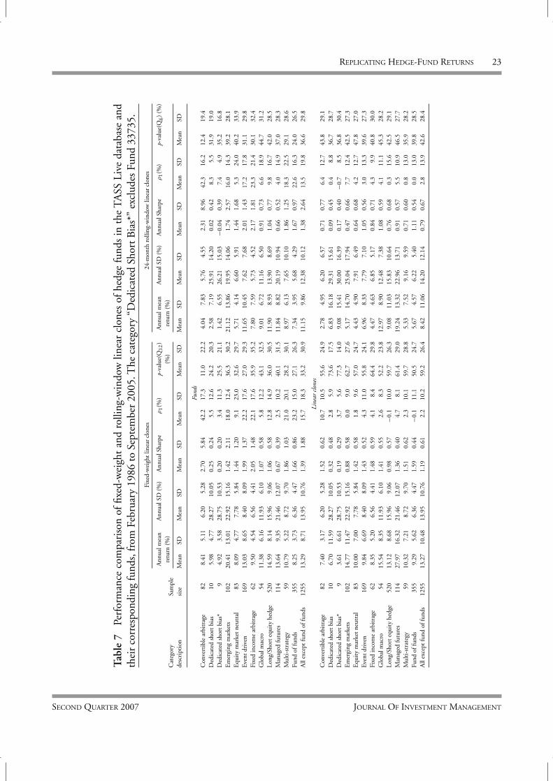
4.2 Performance results

Table 7 contains a comparison between the perfor-mance of fixed-weight and rolling-window linearclones and the original funds from which the clonesare derived.20 The results are striking—for severalcategories, the average mean return of the clones isonly slightly lower than that of their fund counter-parts, and in some categories, the clones do better.For example, the average mean return of the Con-vertible Arbitrage fixed-weight clones is 7.40%, andthe corresponding figure for the funds is 8.41%.For Long/Short Equity Hedge funds, the aver-age mean return for fixed-weight clones and funds

is 13.12% and 14.59%, respectively. And in theMulti-Strategy category, the average mean returnfor fixed-weight clones and funds is 10.32% and10.79%, respectively.

In five cases, the average mean return of thefixed-weight clones is higher than that of thefunds: Dedicated Short Bias (6.70% vs. 5.98%),Equity Market Neutral (10.00% vs. 8.09%), GlobalMacro (15.54% vs. 11.38%), Managed Futures(27.97% vs. 13.64%), and Fund of Funds (9.29%vs. 8.25%). However, these differences are notnecessarily statistically significant because of thevariability in mean returns of funds and cloneswithin their own categories. Even in the case ofManaged Futures, the difference in average meanreturn between fixed-weight clones and funds—almost 15 percentage points—is not significantbecause of the large fluctuations in average meanreturns of the Managed Futures fixed-weight clonesand their corresponding funds (e.g. one standarddeviation of the average mean of the ManagedFutures fixed-weight clones is 16.32% and onestandard deviation of the average mean of the cor-responding sample of funds is 9.35%, accordingto Table 7). Nevertheless, these results suggest thatfor certain categories, the performance of fixed-weight clones may be comparable to that of theircorresponding funds.

On the other hand, at 9.84%, the average perfor-mance of the Event-Driven fixed-weight clones isconsiderably lower than the 13.03% average forthe funds. While also not statistically significant,this gap is understandable given the idiosyncraticand opportunistic nature of most event-drivenstrategies. Moreover, a significant source of the prof-itability of event-driven strategies is the illiquiditypremium that managers earn by providing capitalin times of distress. This illiquidity premium willclearly be missing from a clone portfolio of liquidsecurities, hence we should expect a sizable perfor-mance gap in this case. The same can be said for the



Tab

le7

Perf

orm

ance

com

pari

son

offix

ed-w

eigh

tan

dro

lling

-win

dow

linea

rcl

ones

ofhe

dge

fund

sin

the

TA

SSLi

veda

taba

sean

dth

eir

corr

espo

ndin

gfu

nds,

from

Febr

uary

1986

toSe

ptem

ber

2005

.The

cate

gory

“Ded

icat

edSh

ortB

ias*

”ex

clud

esFu

nd33

735.

Fixe

d-w

eigh

tlin

ear

clon

es24

-mon

thro

lling

-win

dow

linea

rcl

ones

Ann

ualm

ean

Ann

ualS

D(%

)A

nnua

lSha

rpe

ρ1(%

)p-

valu

e(Q

12)

Ann

ualm

ean

Ann

ualS

D(%

)A

nnua

lSha

rpe

ρ1(%

)p-

valu

e(Q

6)

(%)

retu

rn(%

)(%

)re

turn

(%)

Cat

egor

ySa

mpl

ede

scri

ptio

nsi

zeM

ean

SDM

ean

SDM

ean

SDM

ean

SDM

ean

SDM

ean

SDM

ean

SDM

ean

SDM

ean

SDM

ean

SD

Fund

sC

onve

rtib

lear

bitr

age

828.

415.

116.

205.

282.

705.

8442

.217

.311

.022

.24.

047.

835.

764.

552.

318.

9642

.316

.212

.419

.4D

edic

ated

shor

tbia

s10

5.98

4.77

28.2

710

.05

0.25

0.24

5.5

12.6

24.2

20.3

2.58

7.19

25.9

114

.20

0.02

0.42

8.3

5.5

31.9

19.0

Ded

icat

edsh

ortb

ias*

94.

923.

5828

.75

10.5

30.

200.

203.

411

.325

.521

.11.

426.

5526

.21

15.0

3−0

.04

0.39

7.4

4.9

35.2

16.8

Em

ergi

ngm

arke

ts10

220

.41

13.0

122

.92

15.1

61.

422.

1118

.012

.436

.330

.221

.12

13.8

619

.95

14.0

61.

742.

5716

.014

.339

.228

.1E

quit

ym

arke

tneu

tral

838.

094.

777.

785.

841.

441.

209.

123

.032

.629

.75.

714.

146.

605.

911.

441.

685.

324

.040

.233

.9Ev

entd

rive

n16

913

.03

8.65

8.40

8.09

1.99

1.37

22.2

17.6

27.0

29.3

11.6

510

.45

7.62

7.68

2.01

1.43

17.2

17.8

31.1

29.8

Fixe

din

com

ear

bitr

age

629.

504.

546.

564.

412.

051.

4822

.117

.635

.935

.27.

807.

595.

734.

522.

171.

8123

.321

.430

.132

.4G

loba

lmac

ro54

11.3

86.

1611

.93

6.10

1.07

0.58

5.8

12.2

43.1

32.5

9.01

6.72

11.1

66.

500.

910.

736.

618

.944

.731

.2Lo

ng/S

hort

equi

tyhe

dge

520

14.5

98.

1415

.96

9.06

1.06

0.58

12.8

14.9

36.0

30.5

11.9

08.

9313

.90

8.69

1.04

0.77

9.8

16.7

42.0

28.5

Man

aged

futu

res

114

13.6

49.

3521

.46

12.0

70.

670.

392.

510

.240

.131

.511

.84

8.82

20.1

910

.94

0.66

0.52

4.0

14.9

37.0

28.3

Mul

ti-s

trat

egy

5910

.79

5.22

8.72

9.70

1.86

1.03

21.0

20.1

28.2

30.1

8.97

6.13

7.65

10.1

01.

861.

2518

.322

.529

.128

.6Fu

ndof

fund

s35

58.

253.

736.

364.

471.

660.

8623

.215

.027

.126

.37.

343.

955.

684.

291.

670.

9722

.616

.324

.026

.5A

llex

cept

fund

offu

nds

1255

13.2

98.

7113

.95

10.7

61.

391.

8815

.718

.333

.230

.911

.15

9.86

12.3

810

.12

1.38

2.64

13.5

19.8

36.6

29.8

Line

arcl

ones

Con

vert

ible

arbi

trag

e82

7.40

3.17

6.20

5.28

1.52

0.62

10.7

10.5

55.6

24.9

2.78

4.95

6.20

6.57

0.71

0.77

6.4

12.7

43.8

29.1

Ded

icat

edsh

ortb

ias

106.

7011

.59

28.2

710

.05

0.32

0.48

2.8

5.9

73.6

17.5

6.83

16.1

829

.31

15.6

10.

090.

450.

48.

836

.728

.7D

edic

ated

shor

tbia

s*9

3.61

6.61

28.7

510

.53

0.19

0.29

3.7

5.6

77.3

14.0

9.08

15.4

130

.00

16.3

90.

170.

40−0

.78.

536

.830

.4E

mer

ging

mar

kets

102

14.7

711

.47

22.9

215

.16

0.88

0.58

0.0

9.0

62.7

27.6

5.17

14.7

025

.04

17.9

40.

470.

667.

712

.442

.527

.3E

quit

ym

arke

tneu

tral

8310

.00

7.00

7.78

5.84

1.42

0.58

1.8

9.6

57.0

24.7

4.43

4.90

7.91

6.49

0.64

0.68

4.2

12.7

47.8

27.0

Even

tdri

ven

169

9.84

6.69

8.40

8.09

1.43

0.52

4.3

11.0

55.8

24.1

6.96

8.33

7.79

7.10

1.05

0.56

3.0

13.3

39.6

27.3

Fixe

din

com

ear

bitr

age

628.

355.

206.

564.

411.

480.

594.

18.

464

.429

.84.

474.

636.

855.

170.

840.

714.

39.

940

.830

.0G

loba

lmac

ro54

15.5

48.

3511

.93

6.10

1.41

0.55

2.6

8.3

52.2

23.8

12.9

78.

9012

.48

7.38

1.08

0.59

4.1

11.1

45.3

28.2

Long

/Sho

rteq

uity

hedg

e52

013

.12

8.68

15.9

69.

060.

980.

57−0

.110

.059

.726

.39.

0811

.03

15.8

310

.64

0.76

0.68

0.3

15.6

42.5

29.1

Man

aged

futu

res

114

27.9

716

.32

21.4

612

.07

1.36

0.40

4.7

8.1

61.4

29.0

19.2

413

.32

22.9

613

.71

0.91

0.57

5.5

10.9

46.5

27.7

Mul

ti-s

trat

egy

5910

.32

7.21

8.72

9.70

1.51

0.62

2.3

10.1

59.7

28.8

5.33

7.52

9.16

9.59

0.71

0.60

0.8

13.0

35.9

28.2

Fund

offu

nds

355

9.29

5.62

6.36

4.47

1.59

0.44

−0.1

11.1

50.5

24.7

5.67

4.57

6.22

5.40

1.11

0.54

0.0

13.0

39.8

28.5

All

exce

ptfu

ndof

fund

s12

5513

.27

10.4

813

.95

10.7

61.

190.

612.

210

.259

.226

.48.

4211

.06

14.2

012

.14

0.79

0.67

2.8

13.9

42.6

28.4



Emerging Markets fixed-weight clones (14.77%)versus their fund counterparts (20.41%).

For Dedicated Short Bias funds, the difference inaverage mean return between fixed-weight clonesand funds—6.70% and 5.98%, respectively—mayseem somewhat counterintuitive in the light of theexpected-return decomposition in Table 6, wherewe observed that Dedicated Short Bias funds wereresponsible for more than 100% of the averagetotal returns of funds in this category. The factthat Dedicated Short Bias clones have better aver-age performance than the corresponding funds isdue entirely to the clone of a single fund, 33735,and when this outlier is dropped from the sample,the average mean return of the remaining 9 clonesdrops to 3.61% (see the “Dedicated Short Bias∗”row).21 The intuition for the underperformance ofthe fixed-weight clones in this category is clear—given the positive trend in the S&P 500 duringthe 1980s and 1990s, a passive strategy of shortingthe S&P 500 is unlikely to have produced attractivereturns when compared to the performance of morenimble discretionary shortsellers.

The results for the rolling-window clones arebroadly consistent with those of the fixed-weightclones, though the average performance of rolling-window clones is typically lower than that of theirfixed-weight counterparts. For example, the aver-age mean returns of rolling-window clones for allcategories except Dedicated Short Bias are lowerthan their fixed-weight versions, in some cases bya factor of two or three. Part of these differencescan be explained by the different sample periods onwhich rolling-window clones are based—observethat the average mean returns of the underlyingfunds are lower in the rolling-window sample thanin the fixed-weight sample for all categories exceptEmerging Markets. But the more likely sourceof the performance difference between rolling-window and fixed-weight clones is the combinedeffects of look-ahead bias for the fixed-weight clones

and the increased estimation errors implicit in therolling-window clones.

Given these two effects, the performance of therolling-window clones is all the more remark-able in categories such as Dedicated Short Bias(6.83% average mean return vs. 2.58% averagemean return for the corresponding sample of funds),Equity Market Neutral (4.43% clones vs. 5.71%funds), Global Macro (12.97% clones vs. 9.01%funds), Long/Short Equity Hedge (9.08% clonesvs. 11.90% funds), and Managed Futures (19.24%clones vs. 11.84% funds). In the case of Dedi-cated Short Bias funds, it is not surprising thatrolling-window clones are able to outperform bothfixed-weight clones and the funds on which theyare based—the rolling-window feature providesadditional flexibility for capturing time-varyingexpected returns (such as the bull market of the1980s and 1990s) that a fixed-weight strategy sim-ply cannot. And in the case of Managed Futures,as with the fixed-weight clones, the rolling-windowclones exhibit considerable cross-sectional variationin their mean returns hence the superior perfor-mance of clones in this case may not be statisticallysignificant.

Nevertheless, as with fixed-weight clones, rolling-window clones also fall short substantially in thecategories of Emerging Markets (5.17% clonesvs. 21.12% funds), Event Driven (6.96% clonesvs. 11.65% funds), and Fixed Income Arbitrage(4.47% vs. 7.80%). Funds in these categoriesearn part of their expected return from bearingilliquidity risk, which is clearly absent from theclone portfolios constructed with the five factorswe employ. Therefore, we should expect clonesto underperform their fund counterparts in thesecategories.

Another metric of comparison between clones andfunds is the average Sharpe ratio, which adjustsfor the volatilities of the respective strategies. Of



course, given our renormalization process (7), thestandard deviations of the fixed-weight clones areidentical to their fund counterparts, so a compar-ison of Sharpe ratios reduces to a comparison ofmean returns in this case. However, the averageSharpe ratio of a category is not the same as theratio of that category’s average mean return to itsaverage volatility, so the Sharpe ratio statistics inTable 7 and Figure 3 do provide some incrementalinformation. Moreover, for rolling-window clones,there may be some differences in volatilities depend-ing on the time series properties of the underlyingfunds, which makes Sharpe ratio comparisons moreinformative.

The average Sharpe ratio of the fixed-weight sam-ple of Convertible Arbitrage funds is 2.70, which isalmost twice the average Sharpe ratio of 1.52 for thefixed-weight clones, a significant risk-adjusted per-formance gap. Noticeable gaps also exist for EventDriven, Emerging Markets, and Fixed Income Arbi-trage clones versus funds (recall that funds in thesecategories are likely to earn illiquidity risk premianot available to the corresponding clones). How-ever, there is virtually no difference in averageSharpe ratios between fixed-weight clones and fundsin the Dedicated Short Bias, Equity Market Neu-tral, Long/Short Equity Hedge, Multi-Strategy, andFund of Funds categories. And for Global Macroand Managed Futures, the average Sharpe ratiosof the fixed-weight clones are, in fact, higher thanthose of the funds in these categories.

The gaps between average Sharpe ratios of rolling-window clones and those of the underlying fundstend to be more substantial—for the twin reasonscited above—but with some notable exceptions. Onaverage, rolling-window clones in the DedicatedShort Bias, Global Macro, and Managed Futurescategories do better than their fund counterpartson a risk-adjusted basis, with average Sharpe ratiosof 0.09, 1.08, and 0.91, respectively, as com-pared to average Sharpe ratios of 0.02, 0.91, and

0.66, respectively, for the corresponding sampleof funds.

4.3 Liquidity

Table 7 provides another comparison worth noting:the average first-order autocorrelation coefficientsof clones and funds. The first-order autocorrela-tion ρ1 is the correlation between a fund’s currentreturn and the previous month’s return, and Lo(2001, 2002) and Getmansky et al. (2004) observethat positive values for ρ1 in hedge-fund returns isa proxy for illiquidity risk. Table 7 and Figure 4show that the clones have much lower averageautocorrelations than their fund counterparts, withthe exception of Managed Futures for which bothclones and funds have very low average autocorre-lations. For example, the average autocorrelationof Convertible Arbitrage funds in the fixed-weightsample is 42.2%, and the corresponding averagevalue for Convertible Arbitrage fixed-weight androlling-window clones is only 10.7% and 6.4%,respectively. The average autocorrelation of Fundof Funds is 23.2% in the fixed-weight sample, andthe corresponding value for the fixed-weight androlling-window clones is only −0.1% and 0.0%,respectively.

The last two columns of each of the two sub-panels in Table 7 provide a more formal measureof the statistical significance of autocorrelation inthe monthly returns of clones and funds, theLjung–Box Q -statistic, based on the first 12 auto-correlation coefficients in the fixed-weight case andon the first 6 autocorrelation coefficients in therolling-window case.22 Smaller p-values indicatemore statistically significant autocorrelations, andfor every single category, the average p-value ofthe funds is lower than that of the clones. Theseresults confirm our intuition that, by construction,clones are more liquid than their correspondingfunds, highlighting another potential advantage of



Performance Comparison of Clones vs. FundsFixed-Weight Linear Clones

2.70

0.25

0.20

1.42

1.44

1.99

2.05

1.07

1.06

0.67

1.86 1.66

1.39

1.52

0.32 0.19

0.88

1.42

1.43

1.48

1.41

0.98

1.36

1.51

1.59

1.19

0.00

0.50

1.00

1.50

2.00

2.50

3.00


DedicatedShort Bias

DedicatedShort Bias*

EmergingMarkets

EquityMarketNeutral

EventDriven

FixedIncome

Arbitrage

GlobalMacro

Long/ShortEquityHedge

ManagedFutures

Multi-Strategy

Fund ofFunds

All ExceptFund ofFunds

Av

era

ge

Sh

arp

e R

ati

o

Funds Linear Clones

Performance Comparison of Clones vs. Funds24-Month Rolling-Window Linear Clones

2.31

0.02

-0.04

1.74

1.44

2.01

2.17

0.91

1.04

0.66

1.86 1.67

1.38

0.71

0.09

0.17

0.47

0.64

1.05 0.84

1.08

0.76

0.91 0.71

1.11

0.79

-0.50

0.00

0.50

1.00

1.50

2.00

2.50

3.00


DedicatedShort Bias


EmergingMarkets

EquityMarketNeutral

EventDriven

FixedIncome

Arbitrage

GlobalMacro


ManagedFutures

Multi-Strategy

Fund ofFunds


Ave

rag

e S

har

pe

Rat

io

Funds Linear Clones

Figure 3 Comparison of average Sharpe ratios of fixed-weight and 24-month rolling-window linear clonesand their corresponding funds in the TASS Live database, from February 1986 to September 2005. Thecategory “Dedicated Short Bias∗” excludes Fund 33735.



Comparison of Average Autocorrelations of Funds andFixed-Weight Linear Clones

42.2

5.5 3.4

18.0

9.1

22.2

22.1

5.8

12.8

2.5

21.0

23.2

15.7

10.7

2.8

3.7

0.0

1.8

4.3

4.1 2.6

-0.1

4.7 2.3

-0.1

2.2

-5.0

0.0

5.0

10.0

15.0

20.0

25.0

30.0

35.0

40.0

45.0


DedicatedShort Bias


EmergingMarkets

EquityMarketNeutral

EventDriven

FixedIncome

Arbitrage

GlobalMacro


ManagedFutures

Multi-Strategy

Fund ofFunds


Ave

rag

e A

uto

corr

elat

ion

(%

)

Funds Linear Clones

Comparison of Average Autocorrelations of Funds and24-Month Rolling-Window Linear Clones

42.3

8.3

7.4

16.0

5.3

17.2

23.3

6.6

9.8

4.0

18.3

22.6

13.5

6.4

0.4

-0.7

7.7

4.2 3.0

4.3

4.1

0.3

5.5

0.8

0.0

2.8

-5.0

0.0

5.0

10.0

15.0

20.0

25.0

30.0

35.0

40.0

45.0


DedicatedShort Bias


EmergingMarkets

EquityMarketNeutral

EventDriven

FixedIncome

Arbitrage

GlobalMacro


ManagedFutures

Multi-Strategy

Fund ofFunds


Ave

rag

e A

uto

corr

elat

ion

(%

)

Funds Linear Clones

Figure 4 Comparison of average first-order autocorrelation coefficients of fixed-weight and 24-monthrolling-window linear clones and their corresponding funds in the TASS Live database, from February1986 to September 2005. The category “Dedicated Short Bias∗” excludes Fund 33735.



clone portfolios over direct investments in hedgefunds. However, this advantage comes at a cost;as we saw in Section 4.2, the performance gapbetween clones and funds is particularly large forthose categories with the highest levels of illiquidityexposure.

4.4 Leverage ratios

Another consideration in evaluating the practicalsignificance of fixed-weight linear clones is themagnitudes of the renormalization factors γi . Asdiscussed in Section 4.1, these factors representadjustments in the clone portfolios’ leverage so asto yield comparable levels of volatility. If the mag-nitudes are too large, this may render the cloningprocess impractical for the typical investor, who maynot have sufficient credit to support such leverage.The summary statistics in the left panel of Table 8for the renormalization factors {γi} suggest thatthis is not likely to be a concern—the average γiacross all funds in the fixed-weight sample is 2.05,and the median value is 1.81, implying that thetypical amount of additional leverage required toyield fixed-weight clones of comparable volatilityis 81–105% on average, which is far less than theleverage afforded by standard futures contracts suchas the S&P 500.23 For the individual categories, theaverage value of γi for fixed-weight clones variesfrom a low of 1.69 for Fund of Funds to a highof 2.76 for Managed Futures. This accords wellwith our intuition that Fund of Funds is lowerin volatility because of its diversified investmentprofile, and Managed Futures is higher in volatil-ity given the leverage already incorporated into thefutures contracts traded by CTAs and CPOs. Infact, outside of the Managed Futures category, eventhe maximum values for γi are relatively mild—ranging from 2.92 for Convertible Arbitrage to 8.85for Dedicated Short Bias—and the maximum valueof 18.35 for Managed Futures is also reasonablyconservative for that category.

Developing intuition for the leverage ratios for therolling-window clones is slightly more challeng-ing because they vary over time for each clone,so the right panel of Table 8 reports the cross-sectional means and standard deviations of thetime-series means, standard deviations, first-orderautocorrelations, and Q -statistic p-values of eachclone i’s {γit }. For example, the value 1.62 is themean across all rolling-window clones of the time-series-mean leverage ratio of each clone, and thevalue 0.46 is the cross-sectional standard deviation,across all rolling-window clones, of those time-seriesmeans. Table 8 shows that the average time seriesmean leverage ratios for rolling-window clones aresomewhat lower than their fixed-weight counter-parts but roughly comparable, ranging from a lowof 1.38 for Fund of Funds to a high of 1.97 forManaged Futures, with standard deviations of thetime-series means ranging from 0.31 for Fund ofFunds to 0.75 for Dedicated Short Bias (recall thatDedicated Short Bias has only 10 funds, and thatits short-bias mandate during the bull market is alsolikely to create more active rebalancings, contribut-ing to more volatile leverage ratios). However, noneof these leverage ratios fall outside the realm of prac-tical possibility for the five instruments implicit inthe cloning process.

4.5 Equal-weighted clone portfolios

The results in Sections 4.2–4.4 suggest that cloneportfolios consisting primarily of futures and for-ward contracts, properly leveraged, can yield com-parable volatility levels and some of the same riskexposures as certain types of hedge-fund strategies.But these impressions are based on averages of the1610 funds in our sample and their correspond-ing clones, not on specific realizable portfolios. Toaddress this issue, in this section we report thecharacteristics of equal-weighted portfolios of allfixed-weight and rolling-window clones, and com-pare them to the characteristics of equal-weighted



Tab

le8

Sum

mar

yst

atis

tics

for

reno

rmal

izat

ion

fact

orsγ

iof

fixed

-wei

ght

and

24-m

onth

rolli

ng-w

indo

wcl

ones

ofhe

dge

fund

sin

the

TA

SSLi

veda

taba

se,f

rom

Febr

uary

1986

toSe

ptem

ber

2005

.

Fixe

d-w

eigh

tlin

ear

clon

e24

-mon

thro

lling

-win

dow

linea

rcl

one

reno

rmal

izat

ion

fact

orre

norm

aliz

atio

nfa

ctor

TS-

mea

nT

S-SD

ρ1

p-va

lue(

Q6)

Cat

egor

ySa

mpl

ede

scri

ptio

nsi

zeM

inM

edM

ean

Max

SDM

ean

SDM

ean

SDM

ean

SDM

ean

SD

All

fund

s16

100.

111.

812.

0518

.35

0.96

1.62

0.46

0.36

0.28

80.7

14.6

1.9

9.4

Con

vert

ible

arbi

trag

e82

0.11

1.64

1.71

2.92

0.53

1.44

0.40

0.27

0.19

77.1

21.0

3.6

12.6

Ded

icat

edsh

ortb

ias

101.

131.

512.

268.

852.

341.

570.

750.

340.

3682

.412

.20.

92.

8E

mer

ging

mar

kets

102

0.26

1.95

2.13

5.17

0.82

1.68

0.45

0.45

0.38

83.8

10.4

0.5

2.8

Equ

ity

mar

ketn

eutr

al83

0.39

2.17

2.18

4.25

0.80

1.78

0.54

0.40

0.26

77.6

17.4

5.2

17.3

Even

tdri

ven

169

0.40

1.60

1.78

4.45

0.62

1.44

0.36

0.28

0.21

81.5

13.1

1.5

8.2

Fixe

din

com

ear

bitr

age

620.

401.

692.

075.

461.

011.

470.

400.

320.

2179

.014

.92.

912

.2G

loba

lmac

ro54

1.13

2.44

2.60

5.67

1.15

1.86

0.45

0.44

0.34

78.2

17.7

2.0

6.3

Long

/Sho

rteq

uity

hedg

e52

01.

021.

922.

186.

320.

891.

750.

460.

380.

2679

.315

.11.

68.

6M

anag

edfu

ture

s11

41.

172.

412.

7618

.35

1.76

1.97

0.46

0.56

0.37

82.5

12.4

1.3

8.9

Mul

ti-s

trat

egy

590.

451.

892.

043.

750.

751.

570.

460.

380.

3081

.811

.71.

69.

5Fu

ndof

fund

s35

50.

751.

581.

697.

530.

651.

380.

310.

270.

2082

.813

.31.

78.

8



portfolios of the corresponding funds. By includingall clones and funds in each of their respective port-folios, we avoid the potential selection biases thatcan arise from picking a particular subset of clones,

for example, those with particularly high R2s or

statistically significant factor exposures.

Figure 5 plots the cumulative returns of the equal-weighted portfolios of fixed-weight and rolling-window clones, as well as the equal-weightedportfolios of their respective funds and the S&P500. The top panel shows that the equal-weightedportfolio of all fixed-weight clones outperformsboth the equal-weighted portfolio of correspond-ing funds and the S&P 500 over the sample period.However, the bottom panel shows that the perfor-mance of the equal-weighted portfolio of 24-monthrolling-window clones is not quite as impressive,underperforming both the funds portfolio and theS&P 500. However, the clones portfolio underper-forms the S&P 500 only slightly, and apparentlywith less volatility as visual inspection suggests.

Tables 9 and 10 and Figure 6 provide a more detailedperformance comparison of the portfolios of clonesand funds. In particular, Figure 6, which plotsthe Sharpe ratios of the equal-weighted portfoliosof the two types of clones and their correspond-ing funds, for all funds and category by category,shows that for some categories the fixed-weightclone portfolio underperforms the fund portfolio,for example, Dedicated Short Bias (0.09 for theclone portfolio vs. 0.28 for the fund portfolio),Emerging Markets (0.71 clones vs. 1.26 funds),Event Driven (1.89 clones vs. 3.08 funds), FixedIncome Arbitrage (1.79 clones vs. 2.93 funds), andMulti-Strategy (1.62 clones vs. 2.52 funds). How-ever, in other categories, the fixed-weight cloneportfolios have comparable performance and, insome cases, superior performance, for example,Managed Futures, where the fixed-weight cloneportfolio exhibits a Sharpe ratio of 1.80 versus 0.83

for the corresponding fund portfolio. When allclones are used to construct an equal-weighted port-folio, Table 9 reports an annualized mean return of20.44% with an annualized standard deviation of10.23% over the sample period, implying a Sharperatio of 2.00. The annualized mean and standarddeviation for an equal-weighted portfolio of allfunds are 14.76% and 9.06%, respectively, yieldinga Sharpe ratio of 1.63.

The lower panel of Figure 6 provides a compar-ison of the Sharpe ratios of the rolling-windowclone portfolios with their fund counterparts, whichexhibits patterns similar to those of the fixed-weightfund and clone portfolios. The rolling-windowclone portfolios underperform in some categoriesbut yield comparable performance in others, andsuperior performance in the categories of DedicatedShort Bias (0.19 clones vs. 0.12 funds), Equity Mar-ket Neutral (1.42 clones vs. 1.04 funds), GlobalMacro (1.48 clones vs. 1.39 funds), and Fund ofFunds (1.68 clones vs. 1.61 funds). For the equal-weighted portfolio of all rolling-window clones, theaverage return is 12.69% with a standard devia-tion of 10.60%, yielding a Sharpe ratio of 1.20;by comparison, the equal-weighted portfolio of allfunds has a 13.71% average return with a standarddeviation of 8.51%, yielding a Sharpe ratio of 1.61.

Tables 9 and 10 also report skewness, kurtosis, andautocorrelation coefficients for the two types ofclone portfolios, which gives a more detailed char-acterization of the risks of the return streams. Forsome of the categories, the differences in these mea-sures between clones and funds are quite striking.For example, according to Table 9, the portfolio ofFixed Income Arbitrage funds in the fixed-weightcase exhibits a skewness coefficient of −6, a kurtosiscoefficient of 59, and a first-order autocorrelationcoefficient of 27%, implying a negatively skewedreturn distribution with fat tails and significantilliquidity exposure. In contrast, the portfolio ofFixed Income Arbitrage fixed-weight clones has a



Cumulative Return of Equal-Weighted Portfolio of Funds and ClonesFixed-Weight Linear Clones

0

10

20

30

40

50

Feb-86 Feb-88 Feb-90 Feb-92 Feb-94 Feb-96 Feb-98 Feb-00 Feb-02 Feb-04

Funds Linear Clones SP500

Cumulative Return of Equal-Weighted Portfolio of Funds and Clones24-Month Rolling-Window Linear Clones

0

2

4

6

8

10

12

Feb-86 Feb-88 Feb-90 Feb-92 Feb-94 Feb-96 Feb-98 Feb-00 Feb-02 Feb-04

Funds Linear Clones SP500

Figure 5 Cumulative returns of equal-weighted portfolios of funds and fixed-weight and 24-month rolling-window linear clones, and the S&P 500 index, from February 1986 to September 2005.


32 JASMINA HASANHODZIC AND ANDREW W. LOT

able

9Pe

rfor

man

ceco

mpa

riso

nof

equa

l-w

eigh

ted

port

folio

sof

all

fixed

-wei

ght

linea

rcl

ones

vers

usfu

nds

inth

eT

ASS

Live

data

base

,fro

mFe

brua

ry19

86to

Sept

embe

r20

05.

Ded

icat

edsh

ort

Em

ergi

ngE

quit

ym

arke

tA

llfu

nds

Con

vert

ible

arb

bias

mar

kets

neut

ral

Even

tdri

ven

Stat

isti

cFu

nds

Clo

nes

Fund

sC

lone

sFu

nds

Clo

nes

Fund

sC

lone

sFu

nds

Clo

nes

Fund

sC

lone

s

Ann

ualc

ompo

und

retu

rn15

.34

21.8

511

.50

10.1

73.

78−1

.01

22.8

312

.45

13.4

019

.99

14.2

211

.95

Ann

ualiz

edm

ean

14.7

620

.44

11.0

79.

876.

402.

4122

.34

13.6

912

.83

18.6

613

.47

11.5

3A

nnua

lized

SD9.

0610

.23

5.36

5.45

23.2

326

.45

17.7

119

.28

6.23

7.73

4.37

6.11

Ann

ualiz

edSh

arpe

1.63

2.00

2.07

1.81

0.28

0.09

1.26

0.71

2.06

2.41

3.08

1.89

Skew

ness

10

00

00

−1−1

11

−1−1

Kur

tosi

s5

03

22

15

34

18

2ρ

1(≥

20%

inre

d)11

−631

913

336

−31

1232

0ρ

2(≥

20%

inre

d)−1

05

67

−12

−87

−33

1410

4ρ

3(≥

20%

inre

d)−1

10

−4−2

−69

−36

2116

−12

Cor

rela

tion

sto

vari

ous

mar

keti

ndex

es(≥

50%

inre

d,≤

−25%

inre

d):

S&P

500

inde

x44

6948

63−6

6−9

047

886

3758

78M

SCI

Wor

ldin

dex

4059

4252

−71

−92

5181

923

4962

Rus

sell

1000

inde

x44

6849

63−7

0−9

048

886

3660

78R

usse

ll20

00in

dex

4549

5254

−84

−73

5273

−118

7164

NA

SDA

Q10

0st

ock

inde

x38

5342

48−7

8−7

440

743

2652

66B

BA

LIB

OR

USD

3−m

onth

−13

−37

−29

−35

2−1

2−8

−6−8

−29

−8−2

2D

JLe

hman

Bon

dC

omp

GLB

L13

5722

492

7−5

1715

52−6

26U

STr

easu

ryN

/B−1

0−4

6−1

0−3

5−1

6−3

412

7−9

−52

8−1

8G

old

(Spo

t$/o

z)5

−6−9

−1−1

5−8

06

11

−5−7

Oil

(Gen

eric

1st‘

CL’

Futu

re)

−516

−20

−9−1

4−9

−99

1629

−12

US

Dol

lar

spot

inde

x2

−10

61

721

9−1

5−1

52

189

Five

risk

fact

ors

CR

ED

IT3

−920

30−3

9−5

338

55−9

−15

3737

USD

−15

−13

−2−1

3559

−13

−44

−10

14−2

−1B

ON

D13

6324

5810

25−2

911

673

38SP

500

4469

4863

−66

−90

4788

638

5878

DV

IX−2

2−3

2−2

4−4

350

70−3

6−6

46

−21

−50

−50

CM

DT

Y5

27−1

4−1

−12

−13

016

1738

512

CSF

B/T

rem

onti

ndex

esA

llfu

nds

8256

4650

−65

−42

5547

3448

6357

Con

vert

ible

arbi

trag

e47

2679

37−1

9−8

3421

3824

5331

Ded

icat

edsh

ortb

ias

−69

−62

−44

−43

8477

−58

−77

−26

−31

−73

−68

Em

ergi

ngm

arke

ts72

4442

38−6

4−5

894

5521

2460

49E

quit

ym

arke

tneu

tral

5039

3625

−29

−39

2638

5129

3636

Even

tdri

ven

7757

6456

−57

−56

6963

3835

8964

Fixe

din

com

ear

bitr

age

3320

3930

−55

2410

2622

3322

Glo

balm

acro

5436

2636

−25

−628

1722

4331

35Lo

ng/S

hort

equi

tyhe

dge

8261

4347

−79

−58

5564

3639

7160

Man

aged

futu

res

140

−12

−410

17−1

3−1

11

9−1

7−7

Mul

ti-s

trat

egy

2313

2920

−22

−10

013

278

2116


REPLICATING HEDGE-FUND RETURNS 33T

able

9(C

ontin

ued

)Fi

xed-

inco

me

Long

/Sho

rtar

bitr

age

Glo

balm

acro

equi

tyhe

dge

Man

aged

futu

res

Mul

ti-s

trat

egy

Fund

offu

nds

Stat

isti

cFu

nds

Clo

nes

Fund

sC

lone

sFu

nds

Clo

nes

Fund

sC

lone

sFu

nds

Clo

nes

Fund

sC

lone

s

Ann

ualc

ompo

und

retu

rn10

.93

7.91

15.5

624

.90

16.7

917

.40

15.1

538

.37

15.4

315

.08

12.3

018

.74

Ann

ualiz

edm

ean

10.4

87.

7314

.91

22.8

716

.35

17.1

515

.96

34.7

314

.59

14.5

111

.93

17.6

1A

nnua

lized

SD3.

584.

318.

649.

4011

.84

14.0

119

.24

19.3

25.

788.

947.

487.

97A

nnua

lized

Shar

pe2.

931.

791.

732.

431.

381.

220.

831.

802.

521.

621.

592.

21Sk

ewne

ss−6

01

0−2

−11

02

12

0K

urto

sis

593

50

185

20

87

71

ρ1

(≥20

%in

red)

27−2

1717

14−6

59

22−7

205

ρ2

(≥20

%in

red)

135

39

−3−3

−15

−415

−2−8

8ρ

3(≥

20%

inre

d)1

1−7

11−6

2−1

31

1512

−10

−1C

orre

lati

ons

tova

riou

sm

arke

tind

exes

(≥50

%in

red,

≤−2

5%in

red)

:S&

P50

0in

dex

−5−4

1047

7795

−1−2

4371

3166

MSC

IW

orld

inde

x−6

−10

638

6378

−1−2

4460

2949

Rus

sell

1000

inde

x−4

−410

4779

95−3

−244

7131

65R

usse

ll20

00in

dex

22

730

8678

−7−1

345

5332

49N

ASD

AQ

100

Stoc

kin

dex

2−3

333

7278

−7−9

4158

2849

BB

ALI

BO

RU

SD3−

Mon

th−4

−25

−13

−35

−5−1

2−1

3−4

0−1

5−1

9−9

−35

DJ

Lehm

anB

ond

Com

pG

LBL

639

1366

−714

2781

1040

1045

US

Trea

sury

N/B

−8−4

8−1

3−5

88

−7−2

8−8

53

−28

−9−4

0G

old

(Spo

t$/o

z)−1

715

6−1

0−1

113

63

−410

−10

Oil

(Gen

eric

1st‘

CL’

futu

re)

1020

1717

−57

125

921

−217

US

Dol

lar

spot

inde

x11

17−5

−10

178

−14

−27

−6−6

95

Five

risk

fact

ors

CR

ED

IT19

192

029

28−2

4−6

023

182

0U

SD18

32−4

−7−7

−12

−11

−11

−8−1

0−9

7B

ON

D14

6017

782

2123

886

4112

60SP

500

−4−4

1048

7795

−1−1

4371

3166

DV

IX27

00

−28

−56

−61

1318

−28

−45

−9−3

4C

MD

TY

724

1825

318

734

1630

829

CSF

B/T

rem

onti

ndex

esA

llfu

nds

3729

6149

7255

2317

6255

9157

Con

vert

ible

arbi

trag

e48

3226

2837

211

746

2452

28D

edic

ated

shor

tbia

s4

7−2

4−3

5−8

2−7

413

13−5

2−5

5−5

7−5

3E

mer

ging

mar

kets

217

2426

6452

−9−1

150

4070

40E

quit

ym

arke

tneu

tral

−4−1

3628

4641

1812

4737

4835

Even

tdri

ven

2418

3842

7462

−12

−761

5176

54Fi

xed

inco

me

arbi

trag

e79

3718

2521

128

1325

2043

25G

loba

lmac

ro42

3658

4037

2935

2535

3768

40Lo

ng/S

hort

equi

tyhe

dge

128

4242

8965

47

6458

8356

Man

aged

futu

res

−39

408

−7−7

8434

62

162

Mul

ti-s

trat

egy

3522

3113

2011

7−1

3813

2714


34 JASMINA HASANHODZIC AND ANDREW W. LOT

able

10Pe

rfor

man

ceco

mpa

riso

nof

equa

l-w

eigh

ted

port

folio

sof

all2

4-m

onth

rolli

ng-w

indo

wlin

ear

clon

esve

rsus

fund

sin

the

TA

SSLi

veda

taba

se,f

rom

Febr

uary

1986

toSe

ptem

ber

2005

.D

edic

ated

shor

tE

mer

ging

Equ

ity

mar

ket

All

fund

sC

onve

rtib

lear

bbi

asm

arke

tsne

utra

lEv

entd

rive

n

Stat

isti

cFu

nds

Clo

nes

Fund

sC

lone

sFu

nds

Clo

nes

Fund

sC

lone

sFu

nds

Clo

nes

Fund

sC

lone

s

Ann

ualc

ompo

und

retu

rn14

.21

12.8

311

.07

6.88

−0.6

41.

5316

.92

5.34

7.53

12.0

513

.64

10.1

8A

nnua

lized

mea

n13

.71

12.6

910

.71

6.84

3.40

5.92

17.4

38.

587.

5511

.77

12.9

59.

90A

nnua

lized

SD8.

5110

.60

5.79

5.85

27.8

630

.63

18.1

624

.15

7.23

8.26

4.23

5.80

Ann

ualiz

edSh

arpe

1.61

1.20

1.85

1.17

0.12

0.19

0.96

0.36

1.04

1.42

3.06

1.71

Skew

ness

10

01

01

−1−2

−21

−2−1

Kur

tosi

s8

45

36

66

157

212

6ρ

1(≥

20%

inre

d)5

212

−58

−230

73

1436

−6ρ

2(≥

20%

inre

d)−7

−713

9−8

−28

4−1

96

128

ρ3

(≥20

%in

red)

−16

54

−20

24−2

2−1

8−8

−4−2

Cor

rela

tion

sto

vari

ous

mar

keti

ndex

es(≥

50%

inre

d,≤

−25%

inre

d):

S&P

500

inde

x41

5240

61−5

7−7

853

7612

2452

65M

SCI

Wor

ldin

dex

2837

3950

−63

−79

5769

1125

4750

Rus

sell

1000

inde

x41

5242

61−6

1−7

854

7713

2454

66R

usse

ll20

00in

dex

4237

4946

−80

−53

5560

1512

6348

NA

SDA

Q10

0st

ock

inde

x35

4141

46−7

6−6

744

6214

1546

50B

BA

LIB

OR

USD

3-M

onth

−11

−13

−27

−21

3−2

4−5

−4−2

−30

−7−1

6D

JLe

hman

Bon

dC

omp

GLB

L6

2420

313

8−9

112

43−2

16U

STr

easu

ryN

/B−8

−17

−6−2

0−1

4−3

415

12−9

−38

9−1

3G

old

(Spo

t$/o

z)3

3−5

−6−1

47

62

−7−2

5−3

Oil

(Gen

eric

1st‘

CL’

Futu

re)

015

−8−2

−17

−16

−16

818

59

US

Dol

lar

spot

inde

x13

4−2

48

2011

3−1

0−5

1113

Five

risk

fact

ors

CR

ED

IT13

1623

36−3

4−4

542

50−1

1−3

4536

USD

−4−9

−7−3

3044

−20

−16

−75

−64

BO

ND

1430

2037

1229

−44

1051

428

SP50

041

5240

61−5

7−7

853

7612

2452

66D

VIX

−20

−38

−16

−33

4660

−44

−62

−6−1

2−4

1−4

7C

MD

TY

821

−24

−11

−20

76

1326

916

CSF

B/T

rem

onti

ndex

esA

llfu

nds

8356

4939

−81

−27

5847

3337

6357

Con

vert

ible

arbi

trag

e44

3181

30−1

1−3

3421

3120

5333

Ded

icat

edsh

ortb

ias

−67

−66

−44

−47

7956

−59

−69

−28

−32

−72

−63

Em

ergi

ngm

arke

ts69

5040

37−7

1−4

194

5325

2760

51E

quit

ym

arke

tneu

tral

4843

3019

−12

−30

2726

5226

3531

Even

tdri

ven

7561

6248

−60

−38

7067

3736

9064

Fixe

din

com

ear

bitr

age

3423

4526

−4−7

2720

2519

3328

Glo

balm

acro

5835

2926

−39

532

2118

3130

38Lo

ng/S

hort

equi

tyhe

dge

8059

4538

−83

−31

5757

3833

7057

Man

aged

futu

res

18−9

−14

−13

624

−15

−27

511

−17

−10

Mul

ti-s

trat

egy

213

3510

−40

−39

−13

218

209


REPLICATING HEDGE-FUND RETURNS 35T

able

10(C

ontin

ued

)Fi

xed-

inco

me

Long

/Sho

rtar

bitr

age

Glo

balm

acro

equi

tyhe

dge

Man

aged

futu

res

Mul

ti-s

trat

egy

Fund

offu

nds

Stat

isti

cFu

nds

Clo

nes

Fund

sC

lone

sFu

nds

Clo

nes

Fund

sC

lone

sFu

nds

Clo

nes

Fund

sC

lone

s

Ann

ualc

ompo

und

retu

rn8.

604.

5712

.74

17.9

217

.17

12.7

914

.07

14.8

811

.31

8.05

10.7

113

.84

Ann

ualiz

edm

ean

8.36

4.56

12.4

417

.26

16.4

212

.96

14.8

316

.04

10.9

18.

0610

.43

13.3

5A

nnua

lized

SD4.

114.

078.

9511

.66

9.82

13.0

418

.19

20.5

85.

457.

746.

497.

96A

nnua

lized

Shar

pe2.

031.

121.

391.

481.

670.

990.

820.

782.

001.

041.

611.

68Sk

ewne

ss−7

−10

00

−11

00

01

0K

urto

sis

684

31

14

31

22

53

ρ1

(≥20

%in

red)

26−1

48

1217

−11

212

17−1

35

1ρ

2(≥

20%

inre

d)2

−19

−10

83

1−1

4−1

115

91

2ρ

3(≥

20%

inre

d)−6

4−3

8−4

10−1

22

229

−513

Cor

rela

tion

sto

vari

ous

mar

keti

ndex

es(≥

50%

inre

d,≤

−25%

inre

d):

S&P

500

inde

x−9

320

2774

86−5

−844

6134

44M

SCI

Wor

ldin

dex

−9−3

2120

6470

−12

−15

4855

2932

Rus

sell

1000

inde

x−8

321

2777

86−6

−845

6135

45R

usse

ll20

00in

dex

211

2012

8865

−9−9

4644

3630

NA

SDA

Q10

0st

ock

inde

x−1

213

1574

69−1

0−8

4453

2935

BB

ALI

BO

RU

SD3-

Mon

th−6

−11

−17

−21

−9−6

−9−1

2−1

1−2

−11

−12

DJ

Lehm

anB

ond

Com

pG

LBL

512

2327

615

1934

417

925

US

Trea

sury

N/B

−7−2

1−1

9−3

22

−4−2

8−4

22

−13

−9−1

9G

old

(Spo

t$/o

z)2

1014

2−7

−89

108

−58

1O

il(G

ener

ic1s

t‘C

L’Fu

ture

)10

162

13−1

20

517

1528

719

US

Dol

lar

spot

inde

x13

15−1

010

178

−3−3

127

113

Five

Ris

kFa

ctor

sC

RE

DIT

2231

23

2829

−22

−28

2729

1413

USD

1914

−12

0−3

−9−2

−7−9

0−4

−2B

ON

D14

3125

3910

1623

417

2215

33SP

500

−93

2127

7486

−5−8

4361

3445

DV

IX27

−14

−5−1

8−4

8−5

817

8−1

7−4

1−1

3−3

6C

MD

TY

514

515

011

1021

2034

1326

CSF

B/T

rem

onti

ndex

esA

llfu

nds

3421

6143

7352

2514

5841

9055

Con

vert

ible

arbi

trag

e49

2825

3237

241

1244

1846

32D

edic

ated

shor

tbia

s6

−10

−26

−36

−83

−72

131

−43

−52

−56

−59

Em

ergi

ngm

arke

ts15

1329

3363

52−6

−251

3468

46E

quit

ym

arke

tneu

tral

−99

3339

4340

1621

3431

4941

Even

tdri

ven

2427

3540

7461

−12

058

4573

59Fi

xed

inco

me

arbi

trag

e82

2019

2323

1710

727

1539

26G

loba

lmac

ro42

1958

3739

2837

1834

2669

38Lo

ng/S

hort

equi

tyhe

dge

911

4435

8959

411

5844

8153

Man

aged

futu

res

−66

4312

−8−1

483

277

220

−9M

ulti

-str

ateg

y40

1128

518

74

−11

3717

254



Performance comparison of equal-weighted actual-fund vs. clone portfoliosFixed-weight linear clones

1.63

2.07

0.28 0.18

1.26

2.06

3.08 2.93

1.73

1.38

0.83

2.52

1.59

2.00 1.81

0.09

-0.09

0.71

2.41

1.89 1.79

2.43

1.22

1.80 1.62

2.21

-0.50

0.00

0.50

1.00

1.50

2.00

2.50

3.00

3.50

All Funds ConvertibleArbitrage

DedicatedShort Bias


EmergingMarkets

EquityMarketNeutral

Event Driven FixedIncome

Arbitrage

GlobalMacro


ManagedFutures

Multi-Strategy

Fund ofFunds

An

nu

aliz

edS

har

pe

Funds Linear clones

Performance comparison of equal-weighted actual-fund vs. clone portfolios24-month rolling-window linear clones

1.61

1.85

0.12

0.09

0.96

1.04

3.06

2.03

1.39

1.67

0.82

2.00

1.61

1.20

1.17

0.19

0.26

0.36

1.42

1.71

1.12

1.48

0.99

0.78

1.04

1.68

0.00

0.50

1.00

1.50

2.00

2.50

3.00

3.50

All Funds ConvertibleArbitrage

DedicatedShort Bias


EmergingMarkets

EquityMarketNeutral

Event Driven FixedIncome

Arbitrage

GlobalMacro


ManagedFutures

Multi-Strategy

Fund ofFunds

An

nu

aliz

edS

har

pe

Funds Linear clones

Figure 6 Comparison of Sharpe ratios of equal-weighted portfolios of funds versus fixed-weight and 24-month rolling-window linear clones of hedge funds in the TASS Live database, from February 1986 toSeptember 2005.



skewness of 0, a kurtosis of 3, and a first-orderautocorrelation of −2%, and the portfolio of FixedIncome Arbitrage rolling-window clones has simi-lar characteristics, which is consistent with the factthat the clone portfolios are comprised of highlyliquid securities. Other examples of this differ-ence in liquidity exposure include the portfolios offunds in Convertible Arbitrage, Emerging Markets,Event Driven, Multi-Strategy, and Fund of Fundscategories, all of which exhibit significant posi-tive first-order autocorrelation coefficients (31%,36%, 32%, 22%, and 20%, respectively) in con-trast to their fixed-weight clone counterparts (9%,−3%, 0%, −7%, and 5%, respectively). Similarly,the first-order autocorrelations of the portfolios offunds in these five categories using the rolling-window sample (12%, 30%, 36%, 17%, and 5%,respectively) are all larger than their rolling-windowclone counterparts (−5%, 7%, −6%, −13%,and 1%).

While the statistical properties of clone portfoliosmay seem more attractive, it should be kept inmind that some of these characteristics are related toperformance. In particular, one source of negativeskewness and positive kurtosis is the kind of option-based strategies associated with Capital DecimationPartners (see Section 2.1), which is a legitimatesource of expected return. And liquidity exposure isanother source of expected return, as in the case ofFixed Income Arbitrage where one common themeis to purchase illiquid bonds and shortsell more liq-uid bonds with matching nominal cashflows. Byreducing exposures to these risk factors throughclones, we should expect a corresponding reduc-tion in expected return. For example, in the caseof Fixed Income Arbitrage, Table 9 reports thatthe portfolio of funds yields an average return of10.48% with a standard deviation of 3.58% fora Sharpe ratio of 2.93, as compared to the fixed-weight portfolio of clones’ average return of 7.73%with a standard deviation of 4.31% for a Sharperatio of 1.79.

In addition to its expected return and volatility, aportfolio’s correlation with major market indexesis another important characteristic that concernshedge-fund investors because of the diversificationbenefits that alternative investments have tradi-tionally provided. Tables 9 and 10 show that thefixed-weight and rolling-window clone portfoliosexhibit correlations that are similar to those oftheir matching portfolios of funds for a variety ofstock, bond, currency, commodity, and hedge-fundindexes.24 For example, the portfolio of ConvertibleArbitrage funds in the fixed-weight sample has a48% correlation to the S&P 500, a −29% cor-relation to 3-month LIBOR, a 6% correlation tothe US Dollar Index, and a 79% correlation tothe CSFB/Tremont Convertible Arbitrage Index. Incomparison, the portfolio of Convertible Arbitragefixed-weight clones has a 63% correlation to theS&P 500, a −35% correlation to 3-month LIBOR,a 1% correlation to the US Dollar Index, and a37% correlation to the CSFB/Tremont ConvertibleArbitrage Index.

However, some differences do exist. The equal-weighted portfolios of funds tend to have highercorrelation with the corresponding CSFB/TremontHedge-Fund Index of the same category than theequal-weighted portfolios of both types of clones.For example, the correlation between the portfo-lio of funds and the CSFB/Tremont Hedge-FundIndex in the fixed-weight sample is 82%, and thecorresponding correlation for the portfolio of fixed-weight clones with the same index is 56%, and thesame pair of correlations for the rolling-windowcase is 83% and 56%, respectively. This patternis repeated in every single category for both typesof clones, and is not unexpected given that theCSFB/Tremont indexes are constructed from thefunds themselves. On the other hand, the portfoliosof clones are sometimes more highly correlated withcertain indexes than their fund counterparts becauseof how the clones are constructed. For example,the correlation of the portfolio of Equity Market



Table 11 Comparison of signs and absolute differences of correlations of funds and clones to 28market indexes, where fixed-weight and 24-month rolling-window linear clones are constructedfrom hedge funds in the TASS Live database, from February 1986 to September 2005.

Fixed-weight linear clones Rolling-window linear clones

% Same Mean SD % Same Mean SDCategory sign |ρf − ρc| |ρf − ρc| sign |ρf − ρc| |ρf − ρc|All funds 86 19 11 93 12 7Convertible arbitrage 100 12 10 93 12 10Dedicated short bias 93 13 7 89 19 13Emerging markets 79 19 12 86 10 9Equity market neutral 86 19 13 96 12 10Event driven 89 12 10 86 11 6Fixed income arbitrage 86 13 13 71 14 13Global macro 100 20 17 93 10 7Long/Short equity hedge 89 11 6 96 10 6Managed futures 96 15 20 96 9 11Multi-strategy 93 14 10 93 12 6Fund of funds 89 23 11 96 13 9

Neutral fixed-weight clones with the BOND fac-tor is 67%, whereas the correlation of the portfolioof corresponding Equity Market Neutral funds isonly 11%. This difference is likely the result ofthe fact that the BOND factor is one of the fivefactors used to construct clone returns, so the cor-relations of clone portfolios to these factors willtypically be larger in absolute value than those ofthe corresponding fund portfolios.

A summary of the differences in correlation prop-erties between funds and clones is provided byTable 11. The first column in each of the twosub-panels labelled “% Same Sign” contains thepercentage of the 28 market-index correlations inTables 9 and 10, respectively, for which the fundcorrelation and the clone correlation are of the samesign. The next two columns of each sub-panel con-tain the mean and standard deviation of the absolutedifferences in fund- and clone-correlation across the28 market-index correlations. These results show

remarkable agreement in sign for both fixed-weightand rolling-window clones, ranging from 71% to100%, and mean absolute-differences ranging from9% to 23%. And even for the largest mean absolute-difference of 23% (fixed-weight clones in the Fundof Funds category), 89% of the correlations exhibitthe same sign in this category.

Overall, the results in Tables 9–11 show that thecorrelations of clone portfolios are generally com-parable in sign and magnitude to those of the fundportfolios, implying that portfolios of clones canprovide some of the same diversification benefits astheir hedge-fund counterparts.

5 Conclusion

A portion of every hedge fund’s expected return isrisk premia—compensation to investors for bearingcertain risks. One of the most important benefits of



hedge-fund investments is the non-traditional typesof risks they encompass, such as tail risk, liquid-ity risk, and credit risk. Most investors would dowell to take on small amounts of such risks if theyare not already doing so because these factors usu-ally yield attractive risk premia, and many of theserisks are not highly correlated with those of tra-ditional long-only investments. Although talentedhedge-fund managers are always likely to outper-form passive fixed-weight portfolios, the challengesof manager selection and monitoring, the lack oftransparency, the limited capacity of such managers,and the high fees may tip the scales for the institu-tional investor in favor of clone portfolios. In suchcircumstances, portable beta may be a reasonablealternative to portable alpha.

Our empirical findings suggest that the possibil-ity of cloning hedge-fund returns is real. Forcertain hedge-fund categories, the average perfor-mance of clones is comparable—on both a raw-return and a risk-adjusted basis—to their hedge-fund counterparts. For other categories like EventDriven and Emerging Markets, the clones are lesssuccessful.

The differences in performance of clones acrosshedge-fund categories raise an important philo-sophical issue: What is the source of the clones’value-added? One possible interpretation is that thecloning process “reverse-engineers” a hedge fund’sproprietary trading strategy, thereby profiting fromthe fund’s intellectual property. Two assumptionsunderlie this interpretation, both of which arerather unlikely: (1) it is possible to reverse-engineera hedge fund’s strategy using a linear regression of itsmonthly returns on a small number of market-indexreturns; and (2) all hedge funds possess intellec-tual property worth reverse-engineering. Given theactive nature and complexity of most hedge-fundstrategies, it is hard to imagine reverse-engineeringthem by regressing their monthly returns on fivefactors. However, if such strategies have risk

factors in common, it is not hard to imagineidentifying them by averaging a reasonable cross-section of time-series regressions of monthly returnson those risk factors. As for whether all hedgefunds have intellectual property worth reverse-engineering, we have purposely included all theTASS hedge funds in our sample—not just the suc-cessful ones—and it is unlikely that all of the 1610funds possess significant manager-specific alpha.In fact, for our purposes, the main attractionof this sample of hedge funds is the funds’ betaexposures.

Our interpretation of the clones’ value-added is lessdevious: By analyzing the monthly returns of a largecross-section of hedge funds (some of which havegenuine manager-specific alpha, and others whichdo not), it is possible to identify common risk fac-tors from which those funds earn part, but notnecessarily all, of their expected returns. By takingsimilar risk exposures, it should be possible to earnsimilar risk premia from those exposures, hence atleast part of the hedge funds’ expected returns can beattained, but in a lower-cost, transparent, scalable,and liquid manner.

As encouraging as our empirical results may seem,a number of qualifications should be kept in mind.First, we observed a significant performance dif-ference between fixed-weight and rolling-windowclones, and this gap must be weighed carefully inany practical implementation of the cloning pro-cess. The fixed-weight approach yields better histor-ical performance and lower turnover, but is subjectto look-ahead bias so the performance may notbe achievable out-of-sample. The rolling-windowapproach yields less attractive historical perfor-mance, but the simulated performance may be moreattainable, and the flexibility of rolling-windowestimators may be critical for capturing nonsta-tionarities such as time-varying means, volatilities,and regime changes. The costs and benefits of eachapproach must be evaluated on a case-by-case basis



with the specific objectives and constraints of theinvestor in mind.

Second, despite the promising properties of lin-ear clones in several style categories, it is well-known that certain hedge-fund strategies containinherent nonlinearities that cannot be capturedby linear models (see, e.g., Capital Multiplica-tion Partners). Therefore, more sophisticated non-linear methods—including nonlinear regression,regime-switching processes, stochastic volatilitymodels, and Kat and Palaro’s (2005) copula-basedalgorithm—may yield significant benefits in termsof performance and goodness-of-fit. However, thereis an important trade-off between the goodness-of-fit and complexity of the replication process, andthis trade-off varies from one investor to the next.As more sophisticated replication methods are used,the resulting clone becomes less passive, requiringmore trading and risk-management expertise, andeventually becoming as dynamic and complex as thehedge-fund strategy itself.

Third, the replicating factors we proposed are only asmall subset of the many liquid instruments that areavailable to the institutional investor. By expandingthe universe of factors to include options and otherderivative securities, and customizing the set of fac-tors to each hedge-fund category (and perhaps toeach fund), it should be possible to achieve addi-tional improvements in performance, including theability to capture tail risk and other nonlinearitiesin a fixed-weight portfolio. In fact, Haugh and Lo(2001) show that a judiciously constructed fixed-weight portfolio of simple put and call options canyield an excellent approximation to certain dynamictrading strategies, and this approach can be adoptedin our context to create better clones.

Finally, we have not incorporated any transactionscosts or other frictions into our performance anal-ysis of the clone portfolios, which will clearly havean impact on performance. The more passive clones

will be less costly to implement, but they maynot capture as many risk exposures and nonlinear-ities as the more sophisticated versions. However,by construction, clones will have a significant costadvantage over a traditional fund of funds invest-ment, not only because of the extra layer of fees thatfunds of funds typically charge, but also becauseof the clone portfolio’s more efficient use of capi-tal due to the cross-netting of margin requirementsand incentive fees. For example, consider a fundof funds with equal allocations to two managers,each of which charges a 2% management fee and a20% incentive fee, and suppose that in a given year,one manager generates a 25% return and the othermanager loses 5%. Assuming a 1% managementfee and a 10% incentive fee for the fund of funds,and no loss carryforwards for the underlying fundsfrom previous years, this scenario yields a net returnof only 4.05% for the fund of funds investors. Inthis case, the fees paid by the investors amount to astunning 59.5% of the net profits generated by theunderlying hedge funds.

Of course, a number of implementation issuesremain to be resolved before hedge-fund clonesbecome a reality, for example, the estimation meth-ods for computing clone portfolio weights, theimplications of the implied leverage required by ourrenormalization process, the optimal rebalancinginterval, the types of strategies to be cloned, andthe best method for combining clones into a sin-gle portfolio. We are cautiously optimistic that thepromise of our initial findings will provide sufficientmotivation to take on these practical challenges.

Acknowledgments

Research support from AlphaSimplex Group andthe MIT Laboratory for Financial Engineering isgratefully acknowledged. We thank Tom Bren-nan, Nicholas Chan, John Cox, Arnout Eikeboom,Gifford Fong (the editor), Jacob Goldfield, Shane



Haas, Charles Harris, Eric Rosenfeld, KendallWalker, an anonymous referee, and participants atthe CFA Institute Risk Symposium 2006, the Octo-ber 2006 MIT Sloan Leaders Network, and Le ClubB 2006 for many helpful comments.

Notes

1 Nevertheless, derivatives-based replication strategies mayserve a different purpose that is not vitiated by com-plexity: risk attribution, with the ultimate objectiveof portfolio risk management. Even if an underlyinghedge-fund strategy is simpler than its derivatives-basedreplication strategy, the replication strategy may still beuseful in measuring the overall risk exposures of the hedgefund and designing a hedging policy for a portfolio ofhedge-fund investments.

2 As a matter of convention, throughout this paper wedefine the Sharpe ratio as the ratio of the monthly averagereturn to the monthly standard deviation, then annualizeby multiplying by the square root of 12. In the originaldefinition of the Sharpe ratio, the numerator is the excessreturn of the fund, in excess of the risk-free rate. Giventhe time variation in this rate over our sample period, weuse the total return so as to allow readers to select theirown benchmarks.

3 The margin required per contract is assumed to be:

100 × {15% × (current level of the SPX)

− (put premium) − (amount out of the money)}where the amount out of the money is equal to the currentlevel of the SPX minus the strike price of the put.

4 This figure varies from broker to broker, and is meant tobe a rather conservative estimate that might apply to a$10M startup hedge fund with no prior track record.

5 This example was first proposed by Merton in his15.415 Finance Theory class at the MIT Sloan Schoolof Management.

6 During the period from November 1976 to December2004, the annualized mean and standard deviation ofBerkshire Hathaway’s Series A shares were 29.0% and26.1%, respectively, for a Sharpe ratio of 1.12 using 0%for the risk-free benchmark return.

7 Once a hedge fund decides not to report its performance,is liquidated, is closed to new investment, restructured,or merged with other hedge funds, the fund is transferred

into the “Graveyard” database. A hedge fund can only belisted in the “Graveyard” database after being listed in the“Live" database. Because the TASS database fully rep-resents returns and asset information for live and deadfunds, the effects of suvivorship bias are minimized.However, the database is subject to backfill bias—when afund decides to be included in the database, TASS addsthe fund to the “Live” database and includes all availableprior performance of the fund. Hedge funds do not needto meet any specific requirements to be included in theTASS database. Due to reporting delays and time lagsin contacting hedge funds, some Graveyard funds canbe incorrectly listed in the Live database for a period oftime. However, TASS has adopted a policy of transferringfunds from the Live to the Graveyard database if they donot report over an 8- to 10-month period.

8 For studies attempting to quantify the degree and impactof survivorship bias, see Baquero et al. (2005), Brownet al. (1992), Brown et al. (1999), Brown et al. (1997),Carpenter and Lynch (1999), Fung and Hsieh (1997b,2000), Hendricks et al. (1997), Horst et al. (2001), Liang(2000), and Schneeweis and Spurgin (1996).

9 See Posthuma and van der Sluis (2003).10 We are not aware of any studies focusing on this type of

bias, but the impact of selection on statistical inferencehas been explored in some detail by several authors. See,for example, Leamer (1978) and the citations within.

11 TASS defines returns as the change in net asset valueduring the month (assuming the reinvestment of anydistributions on the reinvestment date used by the fund)divided by the net asset value at the beginning of themonth, net of management fees, incentive fees, and otherfund expenses. Therefore, these reported returns shouldapproximate the returns realized by investors.

12 This is no coincidence—TASS is owned by TremontCapital Management, which created the CSFB/Tremontindexes in partnership with Credit Suisse First Boston.

13 It is no coincidence that the categories with the highestdegree of average positive serial correlation are also thecategories with the highest average Sharpe ratios. Smoothreturn series will, by definition, have higher Sharpe ratiosthan more volatile return series with the same mean.

14 Litterman (2005) calls such risk exposures “exotic betas”and argues that “[t]he adjective ‘exotic’ distinguishes itfrom market beta, the only beta which deserves to get paida risk premium.” We disagree—there are several well-established economic models that illustrate the possibilityof multiple sources of systematic risk, each of which com-mands a positive risk premium, for example, Merton



(1973) and Ross (1976). We believe that hedge fundsare practical illustrations of these multi-factor models ofexpected returns.

15 Throughout this paper, all statistics except for thoserelated to the first-order autocorrelation have been annu-alized to facilitate interpretation and comparison.

16 In fact, a decomposition of the total mean returns ofthese two funds shows that the six factors account for verylittle of the two funds’ performance, hence the manager-specific alphas are particularly significant for these twomanagers (see Hasanhodzic and Lo, 2006b, Table 8 fordetails).

17 In Hasanhodzic and Lo (2006a) and in a previous draftof this paper, we used the term “buy-and-hold” todescribe this type of clone. Although this is consistentwith the passive nature of the clone portfolio, it is notstrictly accurate because a portfolio with fixed weightsdoes require periodic rebalancing to maintain those fixedweights. Moreover, if a clone is to be implemented viafutures and forward contracts as we propose, then even inthe absence of portfolio rebalancings, some trading willbe necessary as maturing contracts are “rolled” into thoseof the next maturity date. For these reasons, we now referto clone portfolios with constant portfolio weights overtime as “fixed-weight” clones.

18 However, it should be kept in mind that the futures andforward contracts corresponding to the five factors inEq. (5) have sizable amounts of leverage built into thecontracts themselves, so that for reasonable values of γi ,we can re-write Eq. (9) as:

R̂it = β∗i1 (γiSP500t ) + · · ·

+ β∗i5

(γiCMDTYt

) + δi Rl (14)

= β∗i1 SP500∗

t + · · · + β∗i5 CMDTY∗

t (15)

where we have redefined five new instruments in Eq. (15)that can achieve γi times the leverage of the originalinstruments in (9) at no additional cost. Since the coeffi-cients {β∗

ik} sum to one by construction, there is no needfor any additional borrowing or lending because eachredefined instrument is already leveraged by the factorγi , hence δi ≡0 in Eq. (15).

19 If there are missing observations within this 24-monthwindow, we extend the window backwards in time untilwe obtain 24 datapoints for our regression. Our choiceof 24 months for the rolling window was a compromisebetween the desire to capture nonstationarities in the dataand the need for a sufficient number of observations toestimate the parameters of the clone. We did not try

other window lengths because we wished to reduce theimpact of “backtest bias” or over-fitting on our empiricalresults.

20 Note that each type of clone has its own set of matchingresults for the funds. This is due to the fact that the first 24months of each fund’s history are used to calibrate the ini-tial estimates of the rolling-window clones, hence they arenot included in the rolling-window dataset from whichfund and clone performance statistics are computed.

21 Specifically, fund 33735 has a small but positive SP500beta coefficient, hence the clone portfolio for this fundis long the S&P 500 throughout the sample period fromApril 1997 to March 2005, implying a strong positivecontribution for the SP500 factor. Because the SP500beta coefficient is small and the SP500 factor is the mostvolatile of the five factors, the un-renormalized volatilityof the clone portfolio is considerably smaller than thevolatility of the fund, which causes our renormalizationprocess to magnify the positive mean return of the clonesubstantially.

22 Ljung and Box (1978) propose the following statisticto gauge the significance of the first m autocorrelationcoefficients of a time series with T observations:

Q = T (T +2)m∑

k=1

ρ̂2k/(T −k) (16)

which is asymptotically χ2m under the null hypothesis

of no autocorrelation. By forming the sum of squaredautocorrelations, the statistic Q reflects the absolute mag-nitudes of the ρ̂ks irrespective of their signs, hence fundswith large positive or negative autocorrelation coefficientswill exhibit large Q -statistics.

23 As of July 28, 2006, the initial margin requirement ofthe S&P 500 futures contract that trades on the ChicagoMercantile Exchange is $19,688, with a maintenancemargin requirement of $15,750. Given the contract valueof $250 times the S&P 500 Index and the settlement priceof 1284.30 on July 28, 2006 for the September 2006 con-tract, the initial and maintenance margin requirementsare 6.1% and 4.9% of the contract value, respectively,implying leverage ratios of 16.3 and 20.4, respectively(see http://www.cme.com for further details).

24 Except for the SP500 and DVIX factors, the index returnsused to compute the correlations in Tables 9 and 10are derived solely from the indexes themselves in theusual way (Returnt ≡ (Indext −Indext−1)/Indext ), withno accounting for any distributions. The SP500 factordoes include dividends, and the DVIX factor is the firstdifference of the month-end VIX index.



A Appendix

The following is a list of category descriptions, takendirectly from TASS documentation, that define thecriteria used by TASS in assigning funds in theirdatabase to one of 11 possible categories:

Convertible Arbitrage This strategy is identifiedby hedge investing in the convertible securities of acompany. A typical investment is to be long the con-vertible bond and short the common stock of thesame company. Positions are designed to generateprofits from the fixed income security as well as theshort sale of stock, while protecting principal frommarket moves.

Dedicated Short Bias Dedicated short sellerswere once a robust category of hedge funds beforethe long bull market rendered the strategy difficultto implement. A new category, short biased, hasemerged. The strategy is to maintain net short asopposed to pure short exposure. Short biased man-agers take short positions in mostly equities andderivatives. The short bias of a manager’s portfoliomust be constantly greater than zero to be classifiedin this category.

Emerging Markets This strategy involves equityor fixed income investing in emerging marketsaround the world. Because many emerging mar-kets do not allow short selling, nor offer viablefutures or other derivative products with which tohedge, emerging market investing often employs along-only strategy.

Equity Market Neutral This investment strategyis designed to exploit equity market inefficienciesand usually involves being simultaneously long andshort matched equity portfolios of the same sizewithin a country. Market neutral portfolios aredesigned to be either beta or currency neutral, orboth. Well-designed portfolios typically control forindustry, sector, market capitalization, and other

exposures. Leverage is often applied to enhancereturns.

Event Driven This strategy is defined as “spe-cial situations” investing designed to capture pricemovement generated by a significant pendingcorporate event such as a merger, corporate restruc-turing, liquidation, bankruptcy, or reorganiza-tion. There are three popular sub-categories inevent-driven strategies: risk (merger) arbitrage,distressed/high yield securities, and Regulation D.

Fixed Income Arbitrage The fixed income arbi-trageur aims to profit from price anomalies betweenrelated interest rate securities. Most managers tradeglobally with a goal of generating steady returnswith low volatility. This category includes interestrate swap arbitrage, US and non-US govern-ment bond arbitrage, forward yield curve arbitrage,and mortgage-backed securities arbitrage. Themortgage-backed market is primarily US-based,over-the-counter, and particularly complex.

Global Macro Global macro managers carry longand short positions in any of the world’s major cap-ital or derivative markets. These positions reflecttheir views on overall market direction as influ-enced by major economic trends and/or events. Theportfolios of these funds can include stocks, bonds,currencies, and commodities in the form of cash orderivatives instruments. Most funds invest globallyin both developed and emerging markets.

Long/Short Equity Hedge This directional strat-egy involves equity-oriented investing on both thelong and short sides of the market. The objective isnot to be market neutral. Managers have the abilityto shift from value to growth, from small to mediumto large capitalization stocks, and from a net longposition to a net short position. Managers may usefutures and options to hedge. The focus may beregional, such as long/short US or European equity,or sector specific, such as long and short technologyor healthcare stocks. Long/Short equity funds tend



to build and hold portfolios that are substantiallymore concentrated than those of traditional stockfunds.

Managed Futures This strategy invests in listedfinancial and commodity futures markets and cur-rency markets around the world. The managersare usually referred to as Commodity TradingAdvisors, or CTAs. Trading disciplines are gener-ally systematic or discretionary. Systematic traderstend to use price and market specific information(often technical) to make trading decisions, whilediscretionary managers use a judgmental approach.

Multi-Strategy The funds in this category arecharacterized by their ability to dynamically allocatecapital among strategies falling within severaltraditional hedge-fund disciplines. The use of manystrategies, and the ability to reallocate capitalbetween them in response to market opportunities,means that such funds are not easily assigned to anytraditional category.

The Multi-Strategy category also includes fundsemploying unique strategies that do not fall underany of the other descriptions.

Fund of Funds A “Multi Manager” fund willemploy the services of two or more trading advi-sors or Hedge Funds who will be allocated cash bythe Trading Manager to trade on behalf of the fund.

References

Agarwal, V. and Naik, N. (2000a). “Generalised Style Analysisof Hedge Funds.” Journal of Asset Management 1, 93–109.

Agarwal, V. and Naik, N. (2000b). “On Taking the Alterna-tive Route: Risks, Rewards, and Performance Persistence ofHedge Funds.” Journal of Alternative Investments 2, 6–23.

Agarwal, V. and Naik, N. (2004). “Risk and Portfolio Deci-sions Involving Hedge Funds.” Review of Financial Studies17, 63–98.

Baquero, G., Horst, J. and Verbeek, M. (2005). “Sur-vival, Look-Ahead Bias, and Persistence in Hedge Fund

Performance.” Journal of Financial and Quantitative Analysis40, 493–517.

Bertsimas, D., Kogan, L., and Lo, A. (2001). “Hedg-ing Derivative Securities and Incomplete Markets: Anε-Arbitrage Approach.” Operations Research 49, 372–397.

Brown, S., Goetzmann, W., Ibbotson, R., and Ross, S.(1992). “Survivorship Bias in Performance Studies.” Reviewof Financial Studies 5, 553–580.

Brown, S., Goetzmann, W., and Ibbotson, R. (1999).“Offshore Hedge Funds: Survival and Performance 1989–1995.” Journal of Business 72, 91–118.

Brown, S., Goetzmann, W., and Park, J. (1997). “Conditionsfor Survival: Changing Risk and the Performance of HedgeFund Managers and CTAs.” Yale School of ManagementWorking Paper No. F-59.

Brown, S., Goetzmann, W., and Park, J. (2000). “HedgeFunds and the Asian Currency Crisis.” Journal of PortfolioManagement 26, 95–101.

Capocci, D. and Hubner, G. (2004). “Analysis of Hedge FundPerformance.” Journal of Empirical Finance 11, 55–89.

Carpenter, J. and Lynch, A. (1999). “Survivorship Bias andAttrition Effects in Measures of Performance Persistence.”Journal of Financial Economics 54, 337–374.

Edwards, F. and Caglayan, M. (2001). “Hedge Fund Perfor-mance and Manager Skill.” Journal of Futures Markets 21,1003–1028.

Ennis, R. and Sebastian, M. (2003). “A Critical Look at theCase for Hedge Funds: Lessons from the Bubble.” Journalof Portfolio Management 29, 103–112.

Fung, W. and Hsieh, D. (1997a). “Empirical Characteristicsof Dynamic Trading Strategies: The Case of Hedge Funds.”Review of Financial Studies 10, 275–302.

Fung, W. and Hsieh, D. (1997b). “Investment Style and Sur-vivorship Bias in the Returns of CTAs: The InformationContent of Track Records.” Journal of Portfolio Management24, 30–41.

Fung, W. and Hsieh, D. (2000). “Performance Characteristicsof Hedge Funds and Commodity Funds: Natural vs. Spu-rious Biases.” Journal of Financial and Quantitative Analysis35, 291–307.

Fung, W. and Hsieh, D. (2001). “The Risk in Hedge FundStrategies: Theory and Evidence from Trend Followers.”Review of Financial Studies 14, 313–341.

Fung, W. and Hsieh, D. (2004). “Hedge Fund Benchmarks:A Risk-Based Approach.” Financial Analysts Journal 60,65–80.

Getmansky, M., Lo, A., and Makarov, I. (2004). “An Econo-metric Analysis of Serial Correlation and Illiquidity inHedge-Fund Returns.” Journal of Financial Economics 74,529 –609.



Getmansky, M., Lo, A., and Mei, S. (2004). “SiftingThrough the Wreckage: Lessons from Recent Hedge-Fund Liquidations.” Journal of Investment Management 2,6–38.

Hasanhodzic, J. and Lo, A. (2006a). “Attack of the Clones.”Alpha, June, 54–63.

Hasanhodzic, J. and Lo, A. (2006b). “Can Hedge-FundReturns Be Replicated?: The Linear Case” (August 16,2006). Available at SSRN: <http://ssrn.com/abstract=924565>.

Haugh, M. and Lo, A. (2001). “Asset Allocation andDerivatives.” Quantitative Finance 1, 45–72.

Hendricks, D., Patel, J., and Zeckhauser, R. (1997). “The J-Shape of Performance Persistence Given Survivorship Bias.”Review of Economics and Statistics 79, 161–170.

Hill, J., Mueller, B., and Balasubramanian, V. (2004). “The‘Secret Sauce’ of Hedge Fund Investing—Trading RiskDynamically.” Goldman Sachs Equity Derivatives Strategy,November 2.

Horst, J., Nijman, T., and Verbeek, M. (2001). “EliminatingLook-Ahead Bias in Evaluating Persistence in Mutual FundPerformance.” Journal of Empirical Finance 8, 345–373.

Kat, H. and Palaro, H. 2005, “Who Needs HedgeFunds? A Copula-Based Approach to Hedge Fund ReturnReplication.” Alternative Investment Research CentreWorking paper No. 27, Cass Business School, City Uni-versity, London.

Kat, H. and Palaro, H. (2006a). “Replication and Evaluationof Fund of Hedge Funds Returns.” Alternative InvestmentResearch Centre Working paper No. 28, Cass BusinessSchool, City University, London.

Kat, H. and Palaro, H. (2006b). “Superstars or AverageJoes?: A Replication-Based Performance Evaluation of 1917Individual Hedge Funds.” Alternative Investment ResearchCentre Working paper No. 30, Cass Business School, CityUniversity, London.

Leamer, E. (1978). Specification Searches. New York: JohnWiley and Sons.

Liang, B. (1999). “On the Performance of Hedge Funds.”Financial Analysts Journal, 72–85.

Liang, B. (2000). “Hedge Funds: The Living and the Dead.”Journal of Financial and Quantitative Analysis 35, 309–326.

Litterman, R. (2005). “Beyond Active Alpha.” GoldmanSachs Asset Management.

Ljung, G. and Box, G. (1978). “On a Measure of Lack of Fitin Time Series Models.” Biometrika 65, 297–304.

Lo, A. (2001). “Risk Management For Hedge Funds: Intro-duction and Overview.” Financial Analysts Journal 57,16–33.

Lo, A. (2002). “The Statistics of Sharpe Ratios.” FinancialAnalysts Journal 58, 36–50.

Merton, R. (1973). “An Intertemporal Capital Asset PricingModel.” Econometrica 41, 867–887.

Merton, R. (1981). “On Market Timing and Investment Per-formance I: An Equilibrium Theory of Value for MarketForecasts.” Journal of Business 54, 363–406.

Posthuma, N. and van der Sluis, P. (2003). “A Reality Checkon Hedge Funds Returns” (July 8, 2003). Available atSSRN: <http://ssrn.com/abstract=438840>.

Ross, S. (1976). “The Arbitrage Theory of Capital AssetPricing.” Journal of Economic Theory 13, 341–360.

Schneeweis, T. and Spurgin, R. (1996). “Survivor Biasin Commodity Trading Advisor Performance.” Journal ofFutures Markets 16, 757–772.

Schneeweis, T. and Spurgin, R. (1998). “Multi-Factor Analy-sis of Hedge Fund, Managed Futures, and Mutual FundReturn and Risk Characteristics.” Journal of AlternativeInvestments 1, 1–24.

Sharpe, W. F. (1992). “Asset Allocation: ManagementStyle and Performance Measurement.” Journal of PortfolioManagement 18, 7–19.

Keywords: Hedge fund; portfolio management; riskmanagement


can hedge-fund returns be replicated?: the...

Documents