Can Hedge Funds Time Market Liquidity?*

Charles Cao† Penn State University

Yong Chen‡

Virginia Tech

Bing Liang§ University of Massachusetts at Amherst

Andrew W. Lo**

MIT Sloan School of Management

September 20, 2010

* We thank Andres Almazan, David Bates, Nicole Boyson, Mila Getmansky, Will Goetzmann, Narasimhan Jegadeesh, Bill Kracaw, Lubos Pástor, Andrew Patton, Tarun Ramadorai, Clemens Sialm, Melvyn Teo, and seminar participants at Oxford University, Peking University, University of Massachusetts at Amherst, Virginia Tech, the 2010 Florida State University Finance Conference, and the 2010 China International Conference in Finance for helpful comments. Lubomir Petrasek provided excellent research assistance. Research support from the BNP Paribas Hedge Fund Center at SMU and our respective universities is gratefully acknowledged. † Smeal College of Business, Penn State University, University Park, PA 16802, (814) 865–7891, qxc2@psu.edu. ‡ Pamplin College of Business, Virginia Tech, Blacksburg, VA 24061, (540) 231–4377, yong.chen@vt.edu. § Isenberg School of Management, University of Massachusetts, Amherst, MA 01003, (413) 545–3180, bliang@som.umass.edu. ** MIT Sloan School of Management, Cambridge, MA 02142, (617) 253–0920, alo@mit.edu.

Can Hedge Funds Time Market Liquidity?

Abstract

This paper examines how hedge funds manage their market risk by responding to changes in aggregate liquidity conditions. Using a large sample of equity-oriented hedge funds during the period of 1994–2008, we find strong evidence that hedge-fund managers possess the ability to time market liquidity at both the style category level and the individual fund level. They increase (decrease) their portfolios’ market exposure when equity-market liquidity is high (low). This liquidity timing ability is asymmetric, and depends on market liquidity conditions: hedge funds reduce their portfolios’ market exposure significantly when market liquidity is extremely low, but they do not increase their market exposure when market liquidity is unusually high. Finally, we find that investing in top liquidity timing funds can generate economically significant profits. Our results persist after controlling for alternative benchmark models, various data biases, and return-timing and volatility-timing abilities.

Keywords: Hedge funds, liquidity risk, market liquidity timing, liquidity crisis, bootstrap, investment value JEL Classification: G23, G11

1

1. Introduction

The attempt to generate economic profits through the timing of changes in market

conditions such as returns and volatilities is well known.1 By anticipating such changes, hedge-

fund managers can adjust their portfolio exposures up or down to exploit them. In this paper, we

address a related but previously unexplored question: can hedge funds time market liquidity? In

other words, can fund managers deliver abnormal performance by increasing (decreasing) their

portfolios’ market exposure when market liquidity is high (low)?

The impact of market-wide liquidity shocks on hedge-fund performance and funding

availability is now well-established. Liquidity played a major role in the 1998 Long-Term

Capital Management (LTCM) debacle, in which a global flight-to-quality caused LTCM to

liquidate large positions in the face of margin calls, triggering a market-wide liquidity crisis.

The recent financial crisis also involves liquidity, beginning with the meltdown of the subprime-

mortgage market in 2006–2007, which created a dramatic “liquidity squeeze” in the hedge-fund

industry that generated cascading losses, forced liquidations, and investor redemptions.2 Such

liquidity-based transmission channels have been documented in a recent study by Boyson, Stahel,

and Stulz (2010), who show that large declines in stock-market liquidity can cause contagion in

hedge-fund returns. Therefore, liquidity risk management is critical for hedge funds and other

financial institutions.

If fund managers can correctly forecast market liquidity, they can adjust their portfolio

exposures accordingly to avoid or reduce losses during liquidity squeezes. Hedge funds provide

a natural platform to study managers’ liquidity timing ability. By trading frequently and moving

quickly in between positions, hedge funds are a major provider of liquidity to the markets.3

However, because they are typically leveraged and trade complex instruments, hedge funds are

1 See, for example, Treynor and Mazuy (1966), Henriksson and Merton (1981), Ferson and Schadt (1996), Busse (1999), Bollen and Busse (2001), Jiang, Yao, and Yu (2007), and Chen and Liang (2007). 2 In 2008 alone, total investor redemptions reached nearly $400 billion, and the assets under management by the hedge fund industry have shrunk from a peak of $2.2 trillion in mid-2008 to $1.3 trillion by the end of 2008. See “Hedge Fund Liquidation,” New York Law Journal, March 2, 2009. 3 It is estimated that hedge fund related trading accounts for 25% of the NYSE trading volume. See Black (2004).

2

more easily affected by changes in market liquidity. While the dynamic trading strategies

employed by hedge funds suggest time-varying risk exposures, it is not clear whether hedge

funds pro-actively change market exposures when market liquidity changes.

Using a large sample of equity-oriented hedge funds from the Lipper TASS database

from 1994 to 2008, we find strong evidence that hedge funds exhibit liquidity timing ability at

the portfolio level, i.e., fund managers adjust their portfolios’ market exposure according to the

aggregate liquidity of equity markets. In particular, when market liquidity deviates from its

mean level by one standard deviation, we estimate that a typical hedge fund changes its market

exposure by approximately 17%. Moreover, liquidity timing ability is asymmetric; hedge-fund

managers reduce their portfolios’ market exposure significantly when market liquidity is

extremely low, but do not increase their market exposure when market liquidity is unusually high.

Our evidence is robust to controls for alternative benchmark models, various data biases, and

return-timing and volatility-timing abilities.

At the individual fund level, we find that 14% of our sample funds have significant

liquidity timing ability (at the 5% significance level), and using bootstrap re-sampling techniques,

we confirm that these findings are not attributable to pure luck or sampling variation. We also

investigate the cross-sectional relationship between various fund characteristics and liquidity

timing ability, and find that a fund’s liquidity timing ability is positively associated with the

quality of auditing services, leverage usage, and the managers’ personal capital co-investment,

but negatively associated with management fees. Finally, we gauge the performance

implications of funds with superior liquidity timing ability by measuring the performance of a

portfolio of top liquidity timers. We find that, after adjusting for risk, top liquidity-timing funds

subsequently outperform bottom liquidity-timing funds by about 4.7%–5.9% per year, depending

on the rebalancing interval. In addition, the portfolio of top liquidity-timing funds also

significantly outperforms an equally-weighted portfolio of all funds.

The remaining of the paper is organized as follows. In Section 2, we provide a brief

literature review, and present our method for testing hedge funds’ liquidity timing ability in

3

Section 3. Section 4 contains a description of the hedge-fund data, the market liquidity measure,

and benchmark factors that we use in our empirical analysis. In Section 5, we report evidence of

liquidity timing ability at the style category level. Section 6 contains similar results at the

individual fund level, and also includes evidence on the profitability of investing in top liquidity

timers. We conclude in Section 7.

2. Literature Review

Several recent papers have considered the liquidity risk related to hedge funds.

Brunnermeier and Pedersen (2009) model an asset’s market liquidity and a trader’s funding

liquidity jointly, and stress that the two types of liquidity can mutually reinforce each other and

even cause market-wide liquidity to dry up. Aragon and Strahan (2009) use the event of the

Lehman bankruptcy as an exogenous liquidity shock and show that the Lehman-connected hedge

funds lost funding liquidity and failed twice as much as other funds. Thus, although hedge funds,

in general, provide market liquidity through heavy trading, the liquidity of hedge-fund portfolios

largely depends on market liquidity conditions. Using the Sadka (2006) liquidity risk measure

(which is a variable component of price impact), Sadka (2010) shows that market liquidity risk is

an important determinant in the cross-section of hedge-fund returns. Khandani and Lo (2009) use

cross-sectional regression techniques and autocorrelation-based measures of liquidity to estimate

the liquidity premium in a broad sample of equities, mutual funds, and hedge funds. Teo (2010)

finds that, for liquid hedge funds (i.e., funds imposing less strict redemption terms), investor

redemptions negatively affect fund performance in that funds with high net inflows subsequently

outperform funds with low net inflows.

Despite its obvious importance, the liquidity risk of hedge funds has received

considerably less attention than systemic, operational, and market risk (for details see Chan et al.

(2005), Brown et al (2008) and references thereof).4 Our paper seeks to remedy this gap with its

4 For instance, Chan et al. (2005) study systemic risk and conclude that systemic risk is rising while the hedge fund industry is heading into a challenging period of lower expected returns. Brown et al. (2008) examine operational

4

exclusive focus on the ability of hedge-fund managers to time the market-wide liquidity. It

should be emphasized that we examine the market-wide liquidity instead of the liquidity of assets

held by hedge funds or hedge funds’ funding liquidity.

Second, we present new evidence of hedge funds’ time-varying market exposure. Fung

and Hsieh (1997) show that hedge funds employ dynamic trading strategies that differ from those

used by mutual funds. Agarwal and Naik (2004) find that hedge-fund returns exhibit exposures

to factors built on the payoffs of market index options. Chen and Liang (2007) illustrate that the

market exposure of self-claimed market-timing hedge funds varies with changes in market return

and volatility. Fung, Hsieh, Naik, and Ramadorai (2008) document a structural change in risk

exposures of funds of funds over time. Bollen and Whaley (2009) highlight the importance of

recognizing hedge-fund risk dynamics in evaluating fund performance. Patton and Ramadorai

(2009) characterize time-varying risks using high frequency conditional information. Our work

extends this literature by showing that hedge funds adjust their market exposure according to the

aggregate liquidity conditions.

Finally, the findings of our paper suggest another source of hedge-fund performance.

Given the documented superior performance of hedge funds (e.g., Ackermann, McEnally and

Ravenscraft (1999), Brown, Goetzmann, and Ibbotson (1999), Liang (1999), and Kosowski,

Naik, and Teo (2007)), it is important to identify the sources of fund performance since the

findings can help hedge-fund investors and funds of hedge-fund managers locate their

investment opportunities. Extant studies find a positive association between hedge-fund

performance and incentive fees (Ackermann, McEnally, and Ravenscraft, 1999), redemption

restrictions (Aragon, 2007), managerial incentives (Agarwal, Daniel, and Naik, 2009), and the

proximity of hedge funds to their investment regions (Teo, 2009). Our results suggest that hedge

funds can enhance performance through timing market liquidity.

risk and find that this risk is related to leverage, manager ownership, and conflict of interest issues. They also find that operational risk can largely contribute to the failure of hedge funds even after controlling for investment risk.

5

3. Research Design

In this section we describe the methods to estimate the liquidity timing ability of hedge-

fund managers. In Section 3.1, we define the measure of aggregate market liquidity used to test

for liquidity timing. To control for the effects of other systematic factors, we adopt the Fung and

Hsieh (2004) seven-factor model as our benchmark model in Section 3.2. Our liquidity timing

test is outlined in Section 3.3, and we derive a nonparametric test for individual funds using

bootstrap methods in Section 3.4.

3.1. Measuring Market Liquidity

Liquid markets are generally viewed as those which allow rapid trading with the least

impact on asset prices. We use the equity market liquidity measure developed by Pástor and

Stambaugh (2003)—a cross-sectional average of individual-stock liquidity measures—to

perform our empirical tests. For each stock i listed on the NYSE and AMEX in each month t, we

measure its liquidity using its daily returns and volume by estimating the following regression:

,,...,1 ,)( ,1,,,,,,,,,,,1, ttditditdititditititdi Ddvrsignrr =+×++= ++ εηφθ (1)

where ri,d,t is the excess return of stock i (in excess of the market return) on day d in month t, vi,d,t

is the dollar volume (in millions of dollars) for stock i on day d in month t, and Dt is the number

of trading days in month t. The Pástor-Stambaugh liquidity measure, which is the coefficient ηi,t,

measures the expected return reversal for a given dollar volume, controlling for lagged stock

return. When a stock’s liquidity is low, ηi,t is expected to be negative and large in magnitude.

This measure can be interpreted as volume-related price reversals attributable to liquidity effects,

and is based on the assumption that the lower the liquidity of the stock, the greater the expected

price reversal for a given amount of order flow.5

Two filters are imposed in computing the liquidity measure in each month: (1) A stock

should have at least 15 observations in any given month; and (2) a stock should have a share 5 The intuition for such a measure is straightforward. According to Campbell, Grossman and Wang (1993), risk-averse market makers accommodate order flow from liquidity motivated traders and are compensated with a higher expected return. In (1), order flow is approximated by signed trading volume according to the contemporaneous excess return of stock i. A larger order flow is expected to be associated with a greater compensation; hence liquidity-induced effects on the stock’s expected return are expected to be greater if current volume is higher.

6

price between $5 and $1,000 at the end of the previous month. The Pástor-Stambaugh aggregate

market liquidity measure in month t is then calculated as the average across the individual stocks’

liquidity measures for that month:

∑=

=tN

iti

tt N 1

,1 ηη (2)

where Nt is the number of stocks available in month t. Since the coefficient ηi,t measures an

individual firm’s liquidity cost of trading $1 million of the stock, the market liquidity measure

can be interpreted as the cost of a $1 million trade distributed equally across all sample stocks.

To take into account the fact that the size of the equity market increases over time, we scale each

month’s liquidity measure by the total size of the market at the beginning of the CRSP daily

sample:

tttm mmL η*)/( 1, = (3)

where mt is the total market value of all sample stocks at the end of month t−1, and month 1

refers to August 1962. The scaled and aggregated market liquidity measure, Lm,t, is used in the

subsequent analysis to evaluate hedge funds’ liquidity timing ability. To check the robustness of

our results, in Section 5.6 we also use an alternative market liquidity measure developed by

Hasbrouck (2009).

3.2. Factors in the Benchmark Model

We employ the seven-factor model proposed by Fung and Hsieh (2004) as our

benchmark model for evaluating hedge-fund liquidity timing ability. Among these factors are

two equity-oriented, two bond-oriented, and three primitive trend-following strategy (PTFS)

factors. These factors include: (1) the excess return on the Center for Research in Security Prices

(CRSP) value-weighted market portfolio of all NYSE, AMEX and NASDAQ stocks (MKT); (2)

the Fama-French size factor (SMB);6 (3) the change in the constant-maturity yield on the U.S.

10-year Treasury bond (YLDCHG); (4) the change in the credit spread between Moody’s Baa

6 We consider alternative size factors, such as the spread between the Wilshire Small Cap 1750 index return and the Wilshire Large Cap 750 index return. All our inferences are unchanged.

7

and U.S. 10-year Treasury bonds (BAAMTSY); (5) the return of PTFS bond lookback straddles

(PTFSBD); (6) the return of PTFS currency lookback straddles (PTFSFX); and (7) the return of

PTFS commodity lookback straddles (PTFSCOM). 7 We use our sample of fund returns to

estimate the seven-factor model, and confirm the finding of Fung and Hsieh (2004) that these

factors explain a significant portion of the variation in hedge-fund returns.

3.3. Tests of Liquidity Timing Ability

Among the Fung and Hsieh seven factors, the most important factor for equity-oriented

hedge funds is the excess return on the market portfolio (MKT). For the equally-weighted

portfolio consisting of all 3,156 sample funds, we show that the adjusted from the one-factor

model with the MKT factor is 0.59, which is 85% of the adjusted of 0.69 from the full seven-

factor model (these results are reported in Table 2 and will be discussed more fully in Section 4).

In fact, the ratios of s between the one- and seven-factor models are above 70% for portfolios

of all investment strategies except for Global Macro. These results suggest that the majority of

hedge funds have large exposure to equity market risk. Since market returns and market

liquidity are correlated, we focus our tests on the ability of hedge-fund managers to adjust their

portfolio’s market exposure through timing equity-market liquidity. This test is implemented

with and without controlling hedge funds’ ability to directly time market returns.

The starting point of our liquidity timing analysis is the Fung and Hsieh (2004) seven-

factor model for hedge-fund returns. We assume that hedge funds’ exposure to the market

(MKT) is time-varying and we specify hedge-fund returns as the following:

,,7,6,5,

4,3,2,1,1,,

tptptptp

tptptpttpptp

PTFSCOMPTFSFXPTFSBD

BAAMTSYYLDCHGSMBMKTr

υβββ

ββββα

++++

++++= −

(4)

where , is excess return on fund p in month t. The fund’s market exposure βp,1,t-1 is

determined by the manager at t-1 and varies with her forecast about market liquidity at t if the

manager times market liquidity. In the spirit of Shanken (1990) and Ferson and Schadt (1996),

7 We thank David Hsieh for making the trend-following (PTFS) factor data available on his website http://faculty.fuqua.duke.edu/~dah7/. See Fung and Hsieh (2001) for a description of these factors.

8

we use a Taylor series expansion and specify a fund’s time-varying market beta as a linear

function of the difference between market liquidity and its time-series mean:

),( 1,1,1,1, −− +−+= tmtmpptp uLLγββ (5)

where , is market liquidity in month t and mL is the mean level of market liquidity, βp,1 is the

fund’s average market beta over time, and ut-1 is a zero-mean independent noise term which is

orthogonal to each risk factor. Following the market timing literature (e.g., Admati et al., 1986;

Ferson and Schadt, 1996), we assume that a liquidity timer sets the market beta at t-1 based on

her market-liquidity forecast, equal to the future market liquidity plus noise. While market beta

can be a non-linear function of market liquidity, the linear specification captures the first-order

effect of timing ability. Combining Equations (4) and (5) and letting the noise in market-

liquidity forecast join the error term, we obtain the liquidity timing model:

.)(

,7,6,5,

4,3,2,,1,,

tptptptp

tptptptmtmptpptp

PTFSCOMPTFSFXPTFSBDBAAMTSYYLDCHGSMBMKTLLMKTr

εβββ

βββγβα

++++

+++−++=

(6)

The liquidity-timing measure is the coefficient γ from the above model. We perform our main

test of hedge-fund liquidity timing ability using both portfolio-level and individual fund-level

returns.

3.4. Bootstrap Analysis for Fund-Level Tests

To capture liquidity timing ability at the individual fund level, we need to make

inferences on the cross-sectional statistics (e.g., the top 10th percentile) of individual-fund timing

measures. However, standard parametric inferences do not apply for several reasons. First,

hedge-fund returns of a given strategy are highly correlated, thus the timing measures are not

independent in the cross section. Second, for the majority of our sample funds, the distribution

of the residuals from the liquidity-timing model and the distribution of estimated timing

coefficients are non-normal. Finally, the number of hedge funds in the sample changes over time

and many funds do not have complete return histories, making it difficult to estimate the

covariance matrix of fund returns. Hence, to assess the significance of cross-sectional statistics

9

of liquidity timing measures, we employ a bootstrap analysis as in Bollen and Busse (2001),

Kosowski, Timmermann, White, and Wermers (2006), Jiang, Yao and Yu (2007), Kosowski,

Naik and Teo (2007), and Fama and French (2010). In particular, we implement the following

bootstrap procedure to assess the statistical significance of specific liquidity timing percentiles

and corresponding t-statistics for individual funds:

Step 1: Estimate the Fung and Hsieh seven-factor model for each fund p:

,ˆˆˆ

ˆˆˆˆˆˆ

,7,6,

5,4,3,2,1,,

tptptp

tptptptptpptp

PTFSCOMPTFSFX

PTFSBDBAAMTSYYLDCHGSMBMKTr

εββ

βββββα

+++

+++++=

(7)

and store the estimated coefficients { pa , 1,ˆ

pβ , …….} and the time series of residuals { tp,ε ,

t=1, …..Tp}, where Tp is the number of monthly observations for fund p.

Step 2: Resample the residuals with replacement and obtain a randomly re-sampled residual

time-series { btp,ε }, where b is the index for the bootstrap iteration, b=1,2,…,B. Then

calculate the monthly excess returns of a pseudo fund that, by construction, has no

liquidity timing ability (e.g., 0ˆ =pγ in (6)):

,ˆˆˆ

ˆˆˆˆˆˆ

,7,6,

5,4,3,2,1,,

btptptp

tptptptptppb

tp

PTFSCOMPTFSFX

PTFSBDBAAMTSYYLDCHGSMBMKTr

εββ

βββββα

+++

+++++=

(8)

Step 3: Estimate the liquidity timing model of (6) using the pseudo-fund returns for fund p.

Step 4: Repeat Steps 1–3 for all sample funds and store the cross-sectional statistics of timing

coefficients and their t-statistics.

Step 5: Generate the distributions of the relevant cross-sectional statistics of the timing

coefficients and their t-statistics by repeating Steps 1–4. In our bootstrap analysis, we set

the number of iterations B to be 1,000. Although the pseudo fund has no liquidity

timing ability, the estimated timing coefficient based on its returns can differ from zero

due to sampling variation. Using the bootstrap procedure, we evaluate the distribution

10

of timing measures of the actual sample funds against that of pseudo funds to calculate

the appropriate empirical p-values.

For each cross-sectional statistic of the timing coefficients (or their t-statistics), we

compare its actual estimate with the corresponding distribution of estimates based on the pseudo

funds, and determine whether the liquidity timing coefficients for our sample funds are due to

random sampling variation or fund managers’ timing ability. To conserve space, we focus

exclusively on the t-statistics in our discussion of the bootstrap results in Section 6.

For robustness, we implement three additional bootstrap procedures. In one experiment,

we re-sample the seven factors together but not residuals. In another experiment, we re-sample

the factors and residuals jointly. Finally, we first estimate the liquidity timing regression in (6)

in Step 1, and then remove the liquidity timing term (i.e., the interaction term between market

return and market liquidity condition) in Step 2 to ensure the pseudo funds possess no liquidity

timing skill.

4. The Data

We use two databases to assess hedge-fund liquidity timing ability: the Lipper TASS

hedge-fund database and, for our aggregate liquidity measure, the CRSP daily stock return file.

TASS constitutes one of the most comprehensive hedge-fund databases and provides data on

both active and defunct funds beginning in 1994. The hedge-fund literature has identified

several biases associated with hedge-fund databases, including self-selection bias, survivorship

bias, and backfilling bias (e.g., Brown, Goetzmann and Ibbotson (1999), Fung and Hsieh (2000),

and Liang (2000)). To minimize the impact of these biases, we select the sample funds based on

a few criteria as explained below.

4.1. TASS Data

We start our sample from 1994 and analyze both live and defunct funds. The inclusion of

defunct funds mitigates the impact of survivorship bias. To address the concern that database

11

vendors may backfill funds’ performance when new funds are added—instead of only including

their returns going forward—we exclude the first 12 months of return data for each fund. This

criterion ensures that our findings are robust to backfilling bias.8 Finally, we include funds that

report monthly net-of-fee returns in U.S. dollars and have assets under management (AUM) of at

least $10 million. Smaller funds with AUM less than $10 million are of less concern from an

institutional investor’s perspective, and they have less impact on the market as well. 9 Our

sample period extends from January 1994 through September 2008, and the selection criteria

yields 3,156 equity-oriented hedge funds, comprised of 1,703 live funds and 1,453 defunct funds.

TASS divides funds into the following 11 categories designed to reflect the primary

hedge-fund investment styles: convertible arbitrage, dedicated short bias, event driven, emerging

markets, equity market neutral, fixed income arbitrage, funds of funds, global macro, long-short

equity, managed futures, and multi-strategy. Since our focus is on hedge-fund managers’ ability

to time equity market liquidity, we exclude fixed-income arbitrage and managed-futures funds

from our sample, and also drop funds in the dedicated short-bias strategy because this category

contains only a small number of funds. As a result, there are eight categories in our analyses.

We construct equally-weighted portfolios of: (1) all 3,156 hedge funds (ALL); (2) all

funds excluding funds of hedge funds (ALL-FoF); (3) funds of hedge funds (FoF) only; and (4)

funds in each of the style categories. We evaluate hedge funds’ liquidity timing ability at the

portfolio level as well as at the individual-fund level.

4.2. Summary Statistics

Panel A of Table 1 provides the descriptive statistics of the portfolios’ returns. Over the

period from 1994 to 2008, all hedge funds, including funds of hedge funds, realized an average

return of 0.89% per month (about 11% per year) with a monthly standard deviation of 1.98%.

Typical hedge funds have higher average monthly return (0.98%) in comparison to funds of

8 We do not use the dates when hedge funds were added to TASS data as the cutoff point since funds may be in other databases before they were transferred to TASS. 9 For robustness, we also consider other fund size criteria such as $5 million, and the empirical inferences are unaffected.

12

hedge funds (0.65%), attributed to the double-fee structure of funds of hedge funds (See Brown,

Goetzmann, and Liang (2004)). Among the different hedge-fund strategies, long/short equity

has the highest average monthly return of 1.11% while convertible arbitrage delivers the lowest

average monthly return of 0.62%.

[Insert Table 1 about here.]

According to Getmansky, Lo and Makarov (2004), the first-order autocorrelation of a

hedge fund’s returns can be used as a proxy for the illiquidity of a fund’s assets. Panel A also

reports the first-order autocorrelation of each portfolio’s monthly returns. It reveals that

convertible arbitrage, event driven, and emerging market strategies exhibit a relatively high level

of first-order autocorrelation in monthly returns. This result is consistent with the well-

documented fact that these strategies invest in relatively illiquid securities. We call these

strategies “illiquid strategies”. In contrast, the strategies of global macro and long/short equity

have relatively low first-order autocorrelations, implying that they invest in relatively liquid

securities.10 We call these strategies “liquid strategies”. The remaining three strategies such as

equity market neutral, fund of funds, and multi-strategy carry intermediate-level first-order

autocorrelations, which makes sense as fund of funds and multi-strategy funds have diversified

positions.

Panel B of Table 1 reports summary statistics of our monthly aggregate liquidity measure.

The mean (median) level of market liquidity is −3.2% (−2.4%) per month over the period of

1994–2008, indicating a 3.2% average liquidity cost. To confirm that our measure of market

liquidity is similar to previous measures, we overlay our time series for the 1962–2008 period on

the top of the Pástor and Stambaugh (2003) measure which runs from 1962 to 2000 and find

consistent patterns. 11 The correlation between our liquidity measure and the Pástor and

Stambaugh (2003) measure is 0.98 for the overlapping time period from 1962 to 2000.

10 However, global macro funds can invest in securities of both developed and developing countries. In the latter case, fund assets could be illiquid. 11 Data of the original Pástor and Stambaugh (2003) liquidity measure are available on the Wharton Research Data Services (WRDS).

13

Summary statistics of the Fung-Hsieh seven factors and correlations between the market

liquidity measure and these factors are presented in Panels C and D, respectively. The average

market portfolio excess return is 0.46% per month over the 1994–2008 period, with a standard

deviation of 4.24%; the lowest monthly market excess return is −16.20% in August 1998, and the

highest is 8.18% in April 2003. Meanwhile, the market excess return has a correlation

coefficient of 0.30 with the liquidity measure.

4.3 Adjusted R2s

In Table 2, we present ratios of adjusted R2s from the one- to seven-factor models for

hedge-fund returns. The market factor (MKT) stands out as the most significant; for all hedge

funds excluding funds of funds, the adjusted R2 from the one-factor model is 0.64, which is 87%

of the adjusted R2 from the seven-factor model. For funds of funds, the adjusted R2 from the one-

and seven-factor models are 0.36 and 0.49, respectively. These results motivate us to study

liquidity timing through changes in the equity market beta rather than changes in risk exposures

to the other factors.

[Insert Table 2 about here.]

5. Liquidity Timing at the Portfolio Level

This section reports the evidence on hedge funds’ liquidity timing ability at the portfolio

level. We first present results for the overall portfolio as well as the portfolios of various hedge-

fund strategies. Then we examine liquidity timing ability in extreme market liquidity conditions.

Finally, we check the robustness of the results by employing alternative benchmark models,

controlling for the impact of illiquid holdings, and so forth.

5.1. Liquidity Timing Ability

Based on the liquidity-timing model in (6), Table 3 presents the evidence that hedge

funds adjust their market exposure to changes in market liquidity. The liquidity timing

coefficient of the equally-weighted portfolio of all funds (ALL) is 0.81 and significant at the 1%

level. To put this coefficient in perspective, we compare it with the estimated market beta, i.e.,

14

the coefficient on MKT, from the seven-factor model, which is 0.31.12 If the market liquidity is

above (below) its mean level by one standard deviation (i.e., 0.066 from Table 1), then a typical

hedge fund would increase (decrease) its market exposure accordingly by about 0.053

(0.81×0.066), which is approximately 17% of the fund’s overall market beta based on the seven-

factor model. The result for the portfolio of all hedge funds excluding funds of hedge funds

(ALL-FoF) is qualitatively similar: the timing coefficient is 0.91 with a t-statistic of 3.51. Table

3 also reveals that the liquidity timing coefficient is positive and significant for all strategies

except for equity market neutral. These results provide strong evidence that hedge funds have

liquidity timing ability and that liquidity timing is economically significant. In particular, the

three illiquid strategies we identified in Section 4—convertible arbitrage, event driven, and

emerging markets—are among the strategies with both statistically and economically significant

timing coefficients at the 5% level. This indicates that there is a need to manage liquidity risk in

these illiquid strategies and the managers of these strategies seem to be able to do so. The lack

of liquidity timing with equity-market-neutral funds is also intuitive, since such funds bear

minimal exposure to the market and hence have little incentive to time market liquidity.

[Insert Table 3 about here.]

In the Appendix, we consider whether hedge-fund managers react to lagged market

liquidity conditions by replacing the market liquidity regressor of time t in (6) with its one-period

lagged value. We find that hedge funds do react to recent market liquidity conditions by

changing their market exposure (see Table A.1). However, in contrast to the results of Table 3,

hedge funds holding liquid assets tend to react to past market liquidity strongly, whereas funds

with illiquid holdings seem to time market liquidity actively, due to their need to manage

liquidity risk.

5.2. Liquidity Timing in Extreme Market-Liquidity Conditions

If a hedge-fund manager possesses liquidity timing ability and changes the fund’s market

exposure based on her forecast of market liquidity, then a related question is whether it is more

12 To conserve space, we do not report detailed estimation results from the seven-factor model.

15

important for the fund manager to reduce market exposure during time periods with extremely

poor liquidity conditions (e.g., a market-level liquidity crunch) than to increase market exposure

when the market liquidity level is high. Our next test is designed to examine whether hedge

funds show differential timing ability under extreme liquidity conditions (e.g., bad versus good

liquidity conditions).

We create two indicator variables, D(Low_LIQ)t and D(Hi_LIQ)t and include interactive

terms between the market return and each indicator variable in our tests. D(Low_LIQ)t

(D(Hi_LIQ)t) indicates whether market liquidity in month t belongs to the bottom (top) quintile

during the sample period. Hence, the liquidity-timing regression model is:

,,7,6,5,4,

3,2,2,1,1,, )_(*)_(*

tptptptptp

tptpttpttptpptp

PTFSCOMPTFSFXPTFSBDBAAMTSY

YLDCHGSMBLIQHiDMKTLIQLowDMKTMKTr

εββββ

ββγγβα

+++++

+++++=

(9)

where the coefficients and measure timing ability during extremely low and high liquidity

months.

The results reported in Table 4 suggest that hedge-fund managers adjust their market

exposure asymmetrically. For the equally-weighted portfolio of all sample funds, the estimated

coefficient on the interactive term of the market return with the dummy of low-liquidity months

(  ) is −0.16 and significant at the 1% level. When market liquidity in month t belongs to the

bottom quintile, a typical fund decreases its market exposure significantly, and the net market

beta is roughly 0.15 (= − = 0.31 − 0.16).13 This finding holds for both overall portfolios

and all of the eight category portfolios. The coefficient on the interactive term of market return

with the dummy of high-liquidity months ( ), however, is not significant (except for fund of

funds that has a negative sign on the coefficient). This result is consistent with the finding of

Chen and Liang (2007) that self-proclaimed market-timing hedge funds display better timing

skills when market conditions deteriorate, which reflects a need to hedge against adverse market

circumstances. Therefore, on average hedge funds tend to reduce market exposure when market

13 To keep the table parsimonious, we do not report the beta coefficients, but they are available upon request.

16

liquidity is especially poor, and such adjustments provide investors with some protection against

downside losses from negative liquidity shocks.

[Insert Table 4 about here.]

5.3. Evidence from Alternative Benchmark Models

In this section, we check the robustness of our findings by using an alternative to the

Fung and Hsieh (2004) seven-factor benchmark model. Specifically, we consider the model

proposed by Agarwal and Naik (2004), who construct option-based factors using liquid at-the-

money and out-of-the-money options on the S&P 500 index, and find that these option factors,

together with the Fama-French three factors (e.g., market, size, and value) and a momentum

factor by Carhart (1997), explain the returns on equity-oriented hedge funds quite well. Our

liquidity timing model based on the Agarwal and Naik (2004) benchmark factors is given by:

,

)(

,6,5,

4,3,2,,1,,

tptptp

tptptptmtmptpptp

OTMPUTOTMCALL

UMDHMLSMBMKTLLMKTr

εββ

βββγβα

+++

+++−++=

(10)

where , is the excess return in month t on portfolio p, tSMB , tHML and tUMD are the returns

of the value-weighted, zero-net-investment, factor-mimicking portfolios for size, book-to-market

equity, and one-year momentum in stock returns, tOTMCALL is the out-of-the-money call-

option return factor, and tOTMPUT is the out-of-the-money put-option return factor. The option

factors constructed from the at-the-money and out-of-the-money options are highly correlated;

hence we only employ out-of-the-money option factors to avoid multi-collinearity among these

factors.14

The results reported in Table 5 suggest that our main inference for liquidity timing

remains unchanged when using the alternative benchmark model. The liquidity timing

coefficient is 0.93 and significant at the 1% level for the equally-weighted portfolio of all sample

funds. This estimate is comparable to that reported in Table 3 (0.81) that relies on the Fung and

Hsieh (2004) seven-factor model. The timing coefficient on the equally-weighted portfolio of all

14 We are grateful to Vikas Agarwal and Narayan Naik for providing their option return factors.

17

hedge funds excluding funds of hedge funds is 1.04 with a t-statistic of 3.34. Among the eight

category portfolios, six of them have significant γ coefficients and demonstrate liquidity timing

ability after we control for the option-related factors. We also experiment with other risk factors

(e.g., inclusion of a commodity return index and the Agarwal and Naik at-the-money option

factors) that have been used in the literature to explain hedge-fund returns and find qualitatively

similar results to those presented based on the Fung and Hsieh seven-factor model. Therefore,

our subsequent analysis relies only on the Fung and Hsieh seven-factor model.

[Insert Table 5 about here.]

5.4. The Impact of Illiquid Holdings

Getmansky, Lo, and Makarov (2004) and Aragon (2007) point out that many hedge funds

hold illiquid assets. These illiquid securities do not necessarily trade at the end of each month

and can lead to non-synchronous price reaction. In the absence of end-of-month security

transaction prices, fund managers may use the last transaction price of the month, or have the

flexibility of marking their portfolio for month-end reporting. According to Scholes and

Williams (1977), non-synchronous trading can bias the estimate of a fund’s market beta

downwards. If the bias is systematically related to the market liquidity condition, it could also

bias our inferences about managers’ liquidity timing ability.

To alleviate this potential bias, we incorporate two lagged market excess returns,

MKTt-1 and MKTt-2, as additional control variables in the spirit of Scholes and Williams (1977),

and estimate the following regression model:

,

)(

,7,6,5,4,

3,2,213,112,,11,,

tptptptptp

tptptptptmtmptpptp

PTFSCOMPTFSFXPTFSBDBAAMTSY

YLDCHGSMBMKTMKTMKTLLMKTr

εββββ

ββββγβα

+++++

++++−++= −−

(11)

Table 6 reports the results. For the equally-weighted portfolio of all funds, the estimate of the

liquidity timing coefficient is positive and significant, and MKTt-1 enters the regression strongly,

indicating that hedge funds, in general, do hold relatively illiquid securities. In comparison to

the results reported in Table 3, the equally-weighted portfolios of all funds, all funds excluding

funds of hedge funds, and funds in six of the eight categories still have significant liquidity

18

timing coefficients. In particular, among the categories, emerging market, event driven, funds of

hedge funds, global macro, long/short equity, and multi-strategies still have significant timing

coefficients. Overall, our baseline results of liquidity timing ability presented in Table 3 are

robust after controlling for non-synchronous trading and illiquid holdings.15

[Insert Table 6 about here.]

5.5. Controlling for Return Timing and Volatility Timing

Our test of liquidity timing allows us to examine how hedge funds’ market exposure

varies with market liquidity. However, managers may adjust their funds’ market exposure based

on other information. For example, there is a large literature on the market-timing ability of

professional money managers, dating back to Treynor and Mazuy (1966) and Henriksson and

Merton (1981). The idea of market timing is that the fund manager strategically adjusts the

fund’s market exposure based on her forecast about market returns, increasing (decreasing) the

portfolio’s market exposure when the market goes up (down).

The evidence on mutual fund managers’ market timing ability is mixed. Early studies

find negative timing ability with mutual fund managers. Employing conditional timing models,

Ferson and Schadt (1996) show that mutual funds tend to have neutral market-timing ability.

Bollen and Busse (2001), who use daily returns, and Jiang, Yao, and Yu (2007), who use

information on portfolio holdings, find some positive evidence of market timing in mutual funds.

Moreover, Busse (1999) investigates mutual-fund managers’ volatility-timing ability and finds

evidence that mutual-funds’ market exposures are negatively associated with market volatility.

Recently, Chen and Liang (2007) document evidence of successful return- and volatility-timing

ability using a sample of self-declared market-timing hedge funds.

We re-evaluate hedge-funds’ liquidity timing ability, controlling for both market-return

and volatility timing. We follow Treynor and Mazuy (1966) in controlling for market-return

timing and Busse (1999) for volatility timing, and use the following regression:

15 To check robustness, we use up to 6 lagged market excess returns and re-estimate the liquidity timing model. We find that our conclusion remains unchanged.

19

,

)(*)(

,7,6,5,4,

3,2,2

,1,,

tptptptptp

tptpttptptmtmptpptp

PTFSCOMPTFSFXPTFSBDBAAMTSY

YLDCHGSMBVolVolMKTMKTMKTLLMKTr

εββββ

ββδλγβα

+++++

++−++−++= (12)

where Volt is the market volatility in month t calculated as follows: ,/)( 2,,,∑ −= ttmtdmt NRRVol

Rm,d,t is daily CRSP value-weighted market return on day d in month t, and Nt is the number of

trading days in month t. is the time-series mean of market volatility, and the coefficients γ, λ,

and δ measure liquidity timing, market-return timing, and volatility timing, respectively.

In Table 7 the columns labeled “liquidity timing”, “return timing”, and “volatility timing”

contain the estimates of each timing coefficient. After controlling for market-return and volatility

timing, we find that the coefficient of liquidity timing is still significant for the portfolio of all

sample funds, the portfolio of all hedge funds excluding funds of hedge funds, and six out of

eight category portfolios. For example, the timing coefficient γ is 0.87 (with t-statistic=2.77) and

significant at the 5% level for the portfolio of all funds excluding funds of hedge funds. Hence,

the results confirm the existence of liquidity timing ability, even after controlling for market-

return and volatility timing.

[Insert Table 7 about here.]

5.6 Additional Robustness Checks

We further check the robustness of our findings along four dimensions: the measure of

aggregate liquidity, reverse causality due to the potential impact of changes in funds’ market beta

on future market liquidity, inclusion of the Pástor-Stambaugh liquidity risk factor as an

additional risk factor in the liquidity-timing regression model, and the impact of other

conditioning variables.

Other Liquidity Measures. To ensure that our results are robust to the measure of

aggregate liquidity, we re-examine our timing test using Hasbrouck’s (2009) measure of market

liquidity (multiplied by −1 to make the results comparable to those using the Pástor-Stambaugh

measure).16 Using the Hasbrouck measure and re-estimating (6), we find that for the portfolio of

16 We thank Joel Hasbrouck for making his illiquidity measure available on his website http://pages.stern.nyu.edu/~jhasbrou/research.

20

all sample funds, the liquidity timing coefficient is 0.38 and significant at the 5% level. For the

portfolio of all funds excluding funds of funds, the timing coefficient is also statistically

significant at the 5% level. Further, the liquidity timing coefficients are significant for five of the

eight category portfolios (convertible arbitrage, funds of funds, global macro, long/short equity,

and multi-strategies). Therefore, the Hasbrouck measure delivers similar results to those based

on the Pástor-Stambaugh liquidity measure.

Another issue related to the Pástor-Stambaugh (2003) measure is that the aggregate

liquidity measure is equally weighted across individual stocks. For robustness, we compute a

value-weighted Pástor-Stambaugh liquidity measure and repeat our tests, and the inferences of

liquidity timing ability remain unchanged.

Reverse Causality. Next, we address the concern that the documented liquidity timing

ability may be due to reverse causality, that is, the changes in hedge funds’ market exposure

affect future market liquidity conditions. To check such a possibility, we re-estimate (6) but

replace Lm,t, observed at the end of month t, with next month’s market liquidity condition Lm,t+1.

This specification allows us to examine the relationship of a fund’s market exposure in month t

with market liquidity in month t+1. The regression results show that this relationship is not

significant for each category portfolio or for the overall portfolio of all the funds. Thus, reverse

causality is not likely to explain our findings.

We also examine whether a passive, well-diversified, buy-and-hold portfolio such as the

S&P 500 index fund exhibits liquidity timing ability; if so, our liquidity timing model is clearly

misspecified. Using the S&P 500 index fund returns to estimate the liquidity timing model (6),

we find that the liquidity timing coefficient is not significant at any conventional significance

level.

Inclusion of Liquidity Risk Factor. While our focus in this paper is on hedge funds’

change in market exposure to aggregate liquidity conditions, we check and show that our

findings are robust to including a liquidity risk factor in the benchmark model. In particular, we

follow the approach of Sadka (2010) and Teo (2010) to employ monthly innovation of the Pástor

21

and Stambaugh liquidity measure as the liquidity risk factor, and therefore augment the Fung and

Hsieh seven-factor model with one additional factor. With hedge funds’ liquidity risk controlled,

the liquidity timing coefficient is 0.73 and statistically significant at the 5% level for the overall

portfolio of all funds. For the portfolio of all funds excluding funds of funds, the timing

coefficient is 0.81 (with t-statistic=3.38). Consistent with the results in Table 3, seven out of the

eight category portfolios (with the exception of equity market neutral) have significant liquidity

timing coefficients. Therefore, our results remain unchanged when including a liquidity factor as

an additional risk factor in our baseline regression of Equation (6).

Conditional Liquidity-Timing Model. The essence of strategic timing is the adjustment

of a hedge fund’s market exposure to the manager’s expectations about market conditions of

which liquidity is one important dimension. However, the information set used by the manager

to form her expectations may contain other variables besides her market-liquidity forecast. For

example, in proposing methods for conditional performance evaluation, Ferson and Schadt (1996)

take into account the well-known fact that conditioning information such as aggregate dividend

yield can predict market returns and the market risk premium. To check the robustness of our

liquidity timing results to such conditioning information, we estimate a conditional liquidity-

timing model with four conditioning variables commonly used in the literature: the U.S. three-

month T-bill rate, the term spread between the U.S. 10-year and three-month Treasury securities,

the quality spread between Moody’s BAA- and AAA-rated corporate bonds, and the dividend

yield of the S&P 500 index. The data are obtained from the Federal Reserve Bank and

Datastream. Following Ferson and Schadt (1996), we add interaction terms between the lagged

values of these conditioning variables and the market return to (6).

,

*)(

,7,6,5,4,

3,2,1

1,,1,,

tptptptptp

tptp

q

ltlt

lptmtmptpptp

PTFSCOMPTFSFXPTFSBDBAAMTSY

YLDCHGSMBZMKTMKTLLMKTr

εββββ

βββγβα

+++++

+++−++= ∑=

−

(13)

where Zl,t-1 is the demeaned conditioning variables and q = 4 since we use four conditioning

variables in (13). The results from the conditional liquidity-timing regression are similar to those

based on the unconditional timing model in (6). For instance, for the portfolio consisting of all

22

sample hedge funds, the liquidity timing coefficient is 0.71 and significant at the 5% level. We

also find evidence of significant liquidity-timing coefficient for the portfolio of all funds

excluding funds of funds, and for seven out of the eight category portfolios.

Collectively, our robustness checks suggest that the evidence of liquidity timing ability

among hedge-fund managers is reliable.

6. Evidence at the Individual Fund Level

So far we have presented evidence of hedge-fund liquidity timing ability at the portfolio

level. From the investors’ point of view, another important question is whether one can identify

individual funds that possess liquidity timing ability. In this section, we turn to the evaluation of

liquidity timing at the individual-fund level and show that some hedge funds do possess the skill

to time market liquidity. We also examine the cross-sectional relation between liquidity timing

ability and fund characteristics, and then explore the investment value of identifying hedge funds

with superior liquidity-timing skill. To ensure meaningful estimation of the timing model, we

require each hedge fund to have at least 24 consecutive monthly return observations.17 Since the

first 12 returns are eliminated to avoid backfill bias in the first place, each fund effectively has a

minimum of 36 monthly observations for the current test. This additional requirement reduces

the number of funds in our sample from 3,156 to 2,358.18

6.1. Liquidity Timing of Individual Funds

We estimate the liquidity timing model in (6) for each hedge fund and report cross-

sectional distributions of the estimated coefficients and their associated t-statistics in Table 8.

17 We have also considered the requirement that funds have at least 36 consecutive non-missing monthly returns, and find that our inferences are virtually unchanged. 18 Using this restricted sample, we form equally-weighted portfolios and re-estimate the liquidity timing model of (6). The findings are similar to those reported in Table 3. For example, when we consider the portfolio of all sample funds and the portfolio of all funds excluding funds of funds, the timing coefficients are 0.81 and 0.91 respectively for the unrestricted sample (see Table 3), and 0.91 and 0.98 respectively for the restricted sample with both coefficients significant at the 5% level.

23

Before discussing these results, we examine the percentage of funds with significant liquidity

timing coefficients (γ) to develop intuition for the timing ability of individual funds.

The results in Table 8 suggest that among the 2,358 hedge funds, 14% have positive and

significant γ coefficients at the 5% level, where the null hypothesis is H0: γ=0 and the alternative

hypothesis is Ha: γ>0. For the sample of all funds excluding funds of funds, a similar percentage

of funds show significant timing ability at the 5% level. Across the eight style categories, except

for equity market neutral, all categories have about 10% or more funds with significantly

positive timing coefficients at the 5% level. Emerging market, funds of hedge funds, and

long/short equity funds display stronger results, with more than 15% of funds having significant

timing coefficients at the 5% level.

[Insert Table 8 about here.]

To examine cross-sectional distribution of the estimated timing coefficients, Table 8

presents the 5th, 10th, 15th and 20th percentiles of individual funds’ timing coefficients on both

sides of the distribution. The top 5% of funds with liquidity timing ability have large timing

coefficients. For example, the 5th percentile of the timing coefficient is 3.29 for the overall

sample and 3.78 for the sample excluding funds of funds. The category of funds of funds

contains 652 funds and its top 5% liquidity timers has the smallest timing coefficient (γ =1.35)

among the eight style categories, but this result may be explained by the fact that funds of hedge

funds charge two-tier fees (see Brown, Goetzmann, and Liang (2004)). Among various

categories’ top 5% timing funds, the emerging-market category has the largest timing coefficient

(γ =6.92). This category also contains the largest percentage of funds with significantly positive

timing coefficients (16%). Overall, about 10% or more funds across various categories (except

for equity market neutral) have positive and significant timing coefficients at the 5% level and

these coefficients reveal significant timing ability.

In the Appendix, we show that a large proportion (39%) of individual funds also react to

lagged market liquidity conditions. However, in contrast to the results in Table 8, the percentage

of funds showing significantly negative coefficients for lagged market liquidity is low (3%). The

24

reaction to lagged market liquidity is particularly strong for funds of funds: 64% of them have

positive and significant θ coefficients, suggesting that fund-of-funds managers hold funds that

passively react to market liquidity conditions (see Table A.2 for further details).

6.2. Bootstrap Analysis

We now use the bootstrap procedure, described in Section 3.4, to assess the statistical

significance of the results at the fund level. Table 9 reports the top 5th, 10th, 15th, and 20th

percentiles of t-statistics for timing coefficients and corresponding bootstrapped p-values.

Comparing the actual estimates of the t-statistics ( γt ) with their empirical distributions, we find

that the top-ranked hedge funds’ liquidity timing ability is not due to random sampling variation.

For all funds, the top 5th, 10th, 15th and 20th percentiles of the tγ statistic are 2.46, 1.92, 1.56 and

1.28, respectively, and the p-values associated with these t-statistics are all less than 1%.

Significant liquidity timing coefficients are found for funds in categories such as emerging

market, event driven, fund of funds, and long/short equity.

[Insert Table 9 about here.]

These results suggest that managers of top-ranked funds—as ranked by the significance

of timing coefficients—can time market liquidity. Moreover, for the overall sample and most of

the style categories, bottom-ranked funds (namely, funds that time market liquidity poorly) are

not likely to be due to sampling variation either. This suggests that the market exposure of some

hedge funds mistakenly decreases when market liquidity improves.

For robustness, we implement alternative bootstrap procedures as described in Section

3.4, and find that the results are qualitatively similar to those reported in Table 9. Overall, the

results from the bootstrap analysis indicate that the top-ranked and bottom-ranked liquidity

timing funds are not due to chance, but are most likely attributed to skill and lack thereof.

In the Appendix, we provide additional bootstrap evidence that hedge funds react to

lagged market liquidity in a reasonable way, i.e., fund managers increase market exposure when

the previous month’s market was liquid. This is true at both the overall portfolio level and the

style category level. The large and positive top-ranked t-statistics for the reaction coefficients

25

are not due to random sampling variation, whereas the bootstrap results indicate that the

incidence of unreasonable reaction to recent liquidity conditions (e.g., fund managers increasing

their market exposure when the previous month’s market was illiquid) cannot be distinguished

from random chance (see Table A.3 for further details).

6.3. Liquidity Timing and Fund Characteristics

Next, we analyze the cross-sectional relation between various fund characteristics and

liquidity-timing ability, to determine the types of funds that are more likely to possess timing

skill. Specifically, we regress the liquidity-timing coefficients estimated from (6) on fund

characteristics and fund category indicator variables.

We consider seven fund attributes that have been shown to be associated with hedge-fund

performance: minimum investment requirement, management fee, incentive fee, total redemption

restriction (defined as lock-up period plus redemption advanced notice period), an indicator

variable for effective auditing services (whether the fund provides its auditor’s name and audit

date), an indicator for leverage, and an indicator for whether the fund has its manager’s personal

capital invested, as well as indicators for style categories.19

Table 10 reports the results of the cross-sectional regression. We find that liquidity

timing coefficients are positively associated with such fund attributes as better auditing services,

use of leverage, and the existence of managers’ personal capital co-invested, while negatively

associated with management fees. Management fees may be interpreted as a dead-weight loss to

investment return, so it is not surprising that it is negatively related to timing ability. Effective

auditing, leverage, and a manager’s personal investment may indicate better manager quality and

thus better liquidity-timing skills. In addition, a fund with higher leverage faces more liquidity

risk and requires more skill in managing the portfolio’s risk exposures.

[Insert Table 10 about here.]

19 We do not include fund age and size variables in this test in order to avoid look-ahead bias.

26

6.4. Investment Value of Liquidity Timing

To gauge the practical significance of our liquidity timing measure, we investigate the

investment value of selecting top liquidity timers. To that end, in each month starting from

January 1997, we estimate the liquidity timing coefficient for each fund using the past 36-month

estimation period, and then we form ten hedge fund portfolios based on their liquidity timing

coefficients.20 These portfolios are held subsequently for a 3-, 6-, 9- or 12-month holding period,

and the process is repeated.21 This yields four distinct time series of returns on each portfolio of

various levels of liquidity timing skill. Next we estimate the Fung and Hsieh (2004) seven-factor

model and report each portfolio’s alpha in Table 11.22 Since such investment strategies are most

relevant to fund-of-funds managers, we apply it to two samples: (1) all funds in our sample; and

(2) all funds excluding funds of hedge funds.

[Insert Table 11 about here.]

Table 11 shows that the strategy of investing in top liquidity timers generates risk-

adjusted returns significantly greater than the portfolios of bottom liquidity timers. Depending

on the rebalance interval, the return spread between portfolios of top timers and bottom timers

ranges from 39 to 49 basis points per month (about 4.7%–5.9% per year), both economically and

statistically significant. Similarly, for all hedge funds excluding funds of funds, the return spread

ranges between 4% and 6.6% per year after adjusting for risk. Therefore, the results reveal

substantial investment value associated with liquidity timing ability.

In addition, we compare the performance of investing in top liquidity timers with a

simple alternative strategy of investing in an equally-weighted portfolio of all funds. Again, the

results show significant differences in investment returns. From the perspective a fund-of-funds,

investing in top liquidity-timing funds identified by historical returns can earn superior returns,

20 This portfolios start from January 1997 because we need to use return information from the past three years, and our hedge fund sample begins in January 1994. 21 We use the minimum of 3-month holding period since the average lock-up period for our sample hedge funds is about three months. 22 The results are robust to employing alternative benchmark models as considered in the previous section.

27

as much as 32 basis points per month (or 3.8% per year) higher than the equally-weighted

portfolio of all funds.

In summary, we find a significant difference in alphas between top liquidity timers and

bottom liquidity timers as well as the equally-weighted portfolio of all funds. Interestingly,

when the same investment strategy is applied to funds that are top liquidity reactors—funds with

the largest market-beta adjustment to lagged market liquidity—the differences in alphas vanish

(see Table A.4 of the Appendix for further details). These results may be particularly relevant to

managers of funds of hedge funds seeking to improve their investment process with respect to

liquidity characteristics.

7. Conclusions

In this paper, we examine whether hedge-fund managers possess liquidity timing ability

by adjusting their portfolios’ market exposure as aggregate market liquidity conditions change.

We focus on hedge funds because they are among the most dynamic investment vehicles and

their performance is strongly affected by market liquidity conditions. Using a large sample of

equity-oriented hedge funds over the sample period from 1994 to 2008, we find strong evidence

of liquidity timing at both the style-category level and the individual-fund level.

In particular, hedge-fund managers increase (decrease) their market exposure when the

equity market liquidity is high (low), and this effect is both economically and statistically

significant. Our evidence indicates that funds investing in illiquid securities (such as emerging

market, event driven, and convertible arbitrage funds) and funds with relatively liquid holdings

(such as global macro and long/short equity funds) both demonstrate liquidity timing skills.

However, funds holding liquid assets also react to the past liquidity conditions strongly—their

market exposure is significantly associated with lagged market liquidity.

Also, liquidity timing ability is asymmetric: it is more pronounced when market liquidity

is especially low than when it is especially high. Hedge-fund managers tend to reduce their

portfolios’ market exposures correctly when the market liquidity condition is extremely poor,

28

which helps to protect investors from losses during liquidity crisis. This is important as

institutional investors pay particular attention to preserving capital in such scenarios.

Our bootstrap analysis provides additional evidence of liquidity timing ability at the

individual-fund level. The timing ability of top-ranked liquidity timers cannot be attributed to

sampling variation in our samples of all hedge funds, all funds excluding fund of funds, and

funds in four style categories.

Finally, we find that an investment strategy of investing in top liquidity-timers

significantly outperforms the equally-weighted portfolio of all hedge funds, and apparently

generates economically significant profits, but investing in top liquidity-reactors (those funds

that react to past liquidity conditions) does not. This finding suggests an additional source of

hedge-fund performance, in addition to other sources documented in the literature, such as

incentive structure, share restrictions, and market-return and volatility timing. These empirical

results confirm and extend the common intuition among hedge-fund managers and investors that

liquidity plays a critical role in the dynamics of the hedge-fund industry.

29

Appendix

In this Appendix, we examine whether hedge-fund managers react to lagged market liquidity conditions. Specifically, we use the following regression to test whether fund managers react to the previous month’s market liquidity:

,

)(

,7,6,5,

4,3,2,1,1,,

tptptptp

tptptptmtmptpptp

PTFSCOMPTFSFXPTFSBD

BAAMTSYYLDCHGSMBMKTLLMKTr

εβββ

βββθβα

++++

+++−++= − (A.1)

where Lm,t-1 is the one-month lagged market liquidity measure and the coefficient θ measures reaction to past liquidity conditions. One important difference between this specification and the specification in (6) is that we use lagged market liquidity in the above equation, instead of market liquidity of month t. The logic is that the manager may react to recently observed market liquidity conditions, and such reaction does not need superior information about future market liquidity, but relies on observing recent market-wide liquidity. Another interpretation is that Lm,t-1 belongs to the manager’s conditioning information set, and the manager changes the portfolio’s market beta with conditioning information (see Ferson and Schadt, 1996).

Table A.1 presents evidence at the portfolio level that hedge funds react to recent market liquidity conditions by changing their market exposure. The regression coefficient of the interaction term between the market return and lagged market liquidity is 0.87 for the equally-weighted portfolio of all funds, with a t-statistic of 3.31. In comparison to the results reported in Table 3, none of the three illiquid categories (convertible arbitrage, emerging market, and event driven) shows significant reaction to the previous month’s market liquidity. The two liquid categories (global macro and long/short equity) display large and significant coefficients of 1.53 and 0.96 that are significant at the 5% level, which indicates that hedge funds holding liquid assets tend to react to past market liquidity strongly. In contrast, funds with illiquid holdings tend to time the current market liquidity actively, due to their need to manage liquidity risk.

[Insert Table A.1 about here.]

In Table A.2, we report evidence of individual funds’ reaction to lagged market liquidity conditions. A large proportion (39%) of the funds shows the ability to respond to past market liquidity conditions. In contrast, the percentage of funds showing significantly negative coefficients is low (3%). The evidence of reacting to market liquidity is particularly strong for funds of funds, among which 64% of funds have positive and significant coefficients of θ, suggesting that fund of funds managers invest in funds that passively react to market liquidity conditions. The cross-sectional distribution of the estimated reaction coefficients shows that the global macro category has the largest top 5% reaction coefficient (θ =8.55).

[Insert Table A.2 about here.]

The bootstrap results in Table A.3 provide additional evidence that hedge funds react to recent market liquidity in a reasonable way, namely, fund managers increase market exposure when the previous month’s market was liquid. This is true at both the overall portfolio level and the style category level. The large and positive top-ranked t-statistics for the reaction coefficients are not due to random sampling variation. The bootstrap results suggest that the incidence of unreasonable reaction to recent liquidity conditions (e.g., fund managers increasing their market exposure when the previous month’s market was illiquid) cannot be distinguished from random chance.

[Insert Table A.3 about here.]

Having observed that hedge-fund managers react to the previous month’s market liquidity, we consider whether investing in top-ranked liquidity reactors can produce superior performance. To answer

30

this question, we examine the alphas of portfolios that invest in top liquidity reactors by following a procedure similar to that discussed in Section 6.4. Table A.4 presents the alphas of ten liquidity-reactor portfolios and the return spread between investing in top reactors and bottom reactors. We also compare the portfolio of top reactors with an equally-weighted portfolio of all funds.

[Insert Table A.4 about here.]

Even though hedge-fund managers respond to past liquidity conditions strongly, the portfolios of top liquidity reactors do not outperform bottom liquidity reactors or the equally-weighted portfolio of all funds. For example, for the sample of all hedge funds, the portfolio of top liquidity reactors with a 12-month holding period has a monthly alpha of 0.37%, while the alpha of the equally-weighted portfolio of all funds is 0.40%. These results are in sharp contrast with those reported in Table 11, which shows that investing in top liquidity timers can generate significantly higher alpha.

We can draw a few conclusions from these findings. First, by identifying and investing in top liquidity reactors instead of top liquidity timers, an investor cannot outperform the equally-weighted portfolio of all funds. Second, the group of top liquidity timing funds in Table 11 is not the same as the group of top liquidity reacting funds in Table A.4. Finally, these results reconfirm our earlier finding that liquidity timing ability is attributable to fund managers’ skill and is a source of hedge-fund alpha. Liquidity timing ability and the corresponding fund performance cannot be easily replicated by reacting to past liquidity conditions.

31

References Ackermann, Carl, Richard McEnally, and David Ravenscraft, 1999, The performance of hedge funds: Risk, return and incentives, Journal of Finance 54, 833–874. Admati, Anat R., Sudipto Bhattacharya, Stephen A. Ross, and Paul Pfleiderer, 1986, On timing and selectivity, Journal of Finance 41, 715–730. Agarwal, Vikas, and Narayan Naik, 2004, Risks and portfolio decisions involving hedge funds, Review of Financial Studies 17, 63–98. Agarwal, Vikas, Naveen Daniel and Narayan Naik, 2009, Role of managerial incentives and discretion in hedge fund performance, Journal of Finance 64, 2221–2256. Aragon, George, 2007, Share restrictions and asset pricing: Evidence from the hedge fund industry, Journal of Financial Economics 83, 33–58. Aragon, George, and Philip Strahan, 2009, Hedge funds as liquidity providers: Evidence from the Lehman Bankruptcy. Working paper, Boston College. Billio, Monica, Mila Getmansky, Andrew Lo, and Loriana Pelizzon, 2010, Measuring systemic risk in the finance and insurance sectors. Working paper, University of Massachusetts. Black, Keith, 2004, Managing a hedge fund: A complete guide to trading, business strategies, risk management, and regulations, McGraw Hill. Bollen, Nicolas, and Jeffrey Busse, 2001, On the timing ability of mutual fund managers, Journal of Finance, 1075–1094. Bollen, Nicolas, and Robert Whaley, 2009, Hedge fund risk dynamics: Implications for performance appraisal, Journal of Finance 64, 987–1037. Boyson, Nicole, Christof Stahel, and René Stulz, 2010, Hedge fund contagion and liquidity shocks, Journal of Finance, forthcoming. Brown, Stephen, William Goetzmann, and Roger Ibbotson, 1999, Offshore hedge funds: Survival & performance 1989–95, Journal of Business 72, 91–117. Brown, Stephen, William Goetzmann, and Bing Liang, 2004, Fees on fees in funds of funds, Journal of Investment Management 2, 39–56. Brown, Stephen, William Goetzmann, Bing Liang, and Christopher Schwarz, 2008, Mandatory disclosure and operational risk: Evidence from hedge fund registration, Journal of Finance 63, 2785–2815.

32

Brunnermeier, Markus, and Lasse H. Pedersen, 2009, Market liquidity and funding liquidity, Review of Financial Studies 22, 2201–2238. Busse, Jeffrey, 1999, Volatility timing in mutual funds: evidence from daily returns, Review of Financial Studies 12, 1009–1041. Campbell, John, Sanford Grossman, and Jiang Wang, 1993, Trading volume and serial correlation in stock returns, Quarterly Journal of Economics 108, 905–39. Carhart, Mark, 1997, On persistence of mutual fund performance. Journal of Finance 52, 57–82. Chan, Nicholas, Mila Getmansky, Shane Haas, and Andrew Lo, 2005, Systemic risk and hedge funds, NBER Book Chapter, The Risks of Financial Institutions. Chen, Yong, and Bing Liang, 2007, Do market timing hedge funds time the market? Journal of Financial and Quantitative Analysis 42, 827–856. Fama, Eugene, and Kenneth French, 2010, Luck versus skill in the cross section of mutual fund returns, Journal of Finance, forthcoming. Ferson, Wayne, and Rudi Schadt, 1996, Measuring fund strategy and performance in changing economic conditions, Journal of Finance 51, 425–460. Fung, William, and David Hsieh, 1997, Empirical characteristics of dynamic trading strategies: The case of hedge funds, Review of Financial Studies 10, 275–302. Fung, William, and David Hsieh, 2000, Performance characteristics of hedge funds and CTA funds: Natural versus spurious biases, Journal of Financial and Quantitative Analysis 35, 291–307. Fung, William, and David Hsieh, 2001, The risk in hedge fund strategies: Theory and evidence from trend followers, Review of Financial Studies 14, 313–341. Fung, William, and David Hsieh, 2004, Hedge fund benchmarks: A risk based approach, Financial Analyst Journal 60, 65–80. Fung, William, David Hsieh, Narayan Naik, and Tarun Ramadorai, 2008, Hedge funds: performance, risk, and capital formation, Journal of Finance 63, 1777–1803. Getmansky, Mila, Andrew Lo, and Igor Makarov, 2004, An econometric model of serial correlation and illiquidity in hedge fund returns, Journal of Financial Economics 74, 529–609. Hasbrouck, Joel, 2009, Trading costs and returns for U.S. equities: Estimating effective costs from daily data, Journal of Finance 64, 1445–1477. Henriksson, Roy, and Robert Merton, 1981, On market timing and investment performance II: Statistical procedures for evaluating forecasting skills, Journal of Business 54, 513–534.

33

Jiang, George, Tong Yao and Tong Yu, 2007, Do mutual funds time the market? Evidence from portfolio holdings, Journal of Financial Economics 86, 724–758 Khandani, Amir and Andrew Lo, 2007, What happened to the quants in August 2007? Journal of Financial Markets, forthcoming. Khandani, Amir and Andrew Lo, 2009, Illiquidity premia in asset returns: An empirical analysis of hedge funds, mutual funds, and U.S. equity portfolios, Working paper, MIT. Kosowski, Robert, Narayan Naik, and Melvyn Teo, 2007, Do hedge funds deliver alpha? A Bayesian and bootstrap analysis, Journal of Financial Economics 84, 229–264. Kosowski, Robert, Alan Timmermann, Halbert White, and Russ Wermers, 2006, Can mutual fund “stars” really pick stocks? New evidence from a bootstrap analysis, Journal of Finance 61, 2551–2595. Liang, Bing, 1999, On the performance of hedge funds, Financial Analysts Journal 55, 72–85. Liang, Bing, 2000, Hedge funds: The living and the dead, Journal of Financial and Quantitative Analysis 35, 309–326. Pástor, Lubos, and Robert Stambaugh, 2003, Liquidity risk and expected stock returns, Journal of Political Economy 111, 642–685. Patton, Andrew, and Tarun Ramadorai, 2009, On the dynamics of hedge fund risk exposures, Working paper, Oxford University. Sadka, Ronnie, 2006, Momentum and post-earnings announcement drift anomalies: The role of liquidity risk, Journal of Financial Economics 80, 309-349. Sadka, Ronnie, 2010, Liquidity risk and the cross-section of hedge fund returns, Journal of Financial Economics 98, 54–71. Scholes, Myron, and J. Williams, 1977, Estimating betas from nonsynchronous data, Journal of Financial Economics 5, 309–328. Shanken, Jay, 1990, Intertemporal asset pricing: An empirical investigation, Journal of Econometrics 45, 899–120. Teo, Melvyn, 2009, The geography of hedge funds, Review of Financial Studies 22, 3531–3561. Teo, Melvyn, 2010, The liquidity risk of liquid hedge funds, Journal of Financial Economics, forthcoming. Treynor, Jack, and Kay Mazuy, 1966, Can mutual funds outguess the market? Harvard Business Review 44, 131–136.

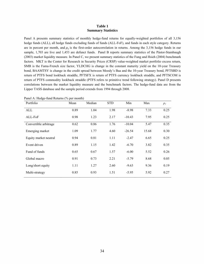
34

Table 1 Summary Statistics

Panel A presents summary statistics of monthly hedge-fund returns for equally-weighted portfolios of all 3,156 hedge funds (ALL), all hedge funds excluding funds of funds (ALL-FoF), and funds in each style category. Returns are in percent per month, and  is the first-order autocorrelation in returns. Among the 3,156 hedge funds in our sample, 1,703 are live and 1,453 are defunct funds. Panel B reports summary statistics of the Pástor-Stambaugh (2003) market liquidity measure. In Panel C, we present summary statistics of the Fung and Hsieh (2004) benchmark factors. MKT is the Center for Research in Security Prices (CRSP) value-weighted market portfolio excess return, SMB is the Fama-French size factor, YLDCHG is change in the constant maturity yield on the 10-year Treasury bond, BAAMTSY is change in the credit spread between Moody’s Baa and the 10-year Treasury bond, PFTSBD is return of PTFS bond lookback straddle, PFTSFX is return of PTFS currency lookback straddle, and PFTSCOM is return of PTFS commodity lookback straddle (PTFS refers to primitive trend following strategy). Panel D presents correlations between the market liquidity measure and the benchmark factors. The hedge-fund data are from the Lipper TASS database and the sample period extends from 1994 through 2008. Panel A: Hedge-fund Returns (% per month)

Portfolio Mean Median STD Min Max ρ1

ALL 0.89 1.04 1.98 -8.98 7.33 0.25

ALL-FoF 0.98 1.23 2.17 -10.43 7.95 0.25

Convertible arbitrage 0.62 0.86 1.76 -10.04 5.47 0.35

Emerging market 1.09 1.77 4.60 -26.54 15.68 0.30

Equity market neutral 0.94 0.81 1.11 -2.47 6.65 0.25

Event driven 0.89 1.15 1.42 -6.70 3.82 0.35

Fund of funds 0.65 0.67 1.57 -6.00 5.52 0.26

Global macro 0.91 0.73 2.21 -5.79 8.68 0.05

Long/short equity 1.11 1.27 2.60 -9.63 9.36 0.19

Multi-strategy 0.85 0.93 1.51 -5.95 5.92 0.27

35

Table 1 (Continued)

Panel B: Liquidity Measure (%) Mean Median STD Min Max

P-S liquidity measure -3.22 -2.38 6.56 -27.44 19.24

Panel C: Fung and Hsieh Benchmark Factors

Mean Median STD Min Max

MKT 0.46 1.03 4.24 -16.20 8.18

SMB 0.17 -0.17 3.78 -16.79 21.96 YLDCHG -0.01 -0.04 0.23 -0.53 0.65

BAAMTSY 0.01 -0.02 0.21 -0.47 1.57

PTFSBD -1.22 -3.86 14.53 -25.36 68.86

PTFSFX 0.41 -2.93 19.34 -30.13 90.27

PTFSCOM -0.04 -2.54 13.91 -24.20 64.75 Panel D: Correlations

Liquidity MKT SMB YLDCHG BAAMTSY PFTSBD PTFSFX PTFSCOM

1.00

0.30 1.00

0.03 0.20 1.00

-0.01 0.12 0.18 1.00

-0.13 -0.21 0.10 0.70 1.00

-0.07 -0.16 -0.03 0.04 0.15 1.00

-0.10 -0.12 0.02 -0.11 0.06 0.19 1.00

0.01 -0.11 -0.01 -0.02 0.13 0.18 0.33 1.00

36

Table 2 Ratios of Adjusted s from One-factor and Seven-factor Models for Hedge-Fund Returns

Time series regression of one-factor and seven-factor models for hedge-fund excess returns:

,,1,, tptpptp MKTr εβα ++=

.,7,6,5,

4,3,2,1,,

tptptptp

tptptptpptp

PTFSCOMPTFSFXPTFSBD

BAAMTSYYLDCHGSMBMKTr

εβββ

ββββα

++++

++++=

The dependent variable is the monthly excess return on an equally-weighted portfolio of all sample hedge funds (ALL), all hedge funds excluding funds of funds (ALL-FoF), or funds in each style category. The independent variables include the Fung and Hsieh (2004) factors: MKT is the Center for Research in Security Prices (CRSP) value-weighted market portfolio excess return, SMB is the Fama-French size factor, YLDCHG is change in the constant maturity yield on the 10-year Treasury bond, BAAMTSY is change in the credit spread between Moody’s Baa and the 10-year Treasury bond, PFTSBD is return of PTFS bond lookback straddle, PFTSFX is return of PTFS currency lookback straddle, and PFTSCOM is return of PTFS commodity lookback straddle (PTFS refers to primitive trend following strategy).

Portfolios

(1-factor model) t-statistic

Adj. R2

(1-factor model)

Ratio of R2s

(1-factor/7-factor)

ALL 0.36 10.90 0.59 0.85

ALL-FoF 0.41 11.43 0.64 0.87

Convertible arbitrage 0.24 5.87 0.34 0.71

Emerging market 0.67 6.33 0.37 0.85

Equity market neutral 0.08 4.70 0.10 0.68

Event driven 0.23 7.38 0.48 0.77

Fund of funds 0.22 7.85 0.36 0.73

Global macro 0.19 5.46 0.13 0.46

Long/short equity 0.51 17.03 0.71 0.87

Multi-strategy 0.26 9.97 0.52 0.89

37

Table 3 Liquidity Timing Ability: Portfolio-Level Evidence

This table presents results from the liquidity timing regression model:

,)( ,7,6,5,4,3,2,,1,, tptptptptptptptmtmptpptp PTFSCOMPTFSFXPTFSBDBAAMTSYYLDCHGSMBMKTLLMKTr εββββββγβα +++++++−++= where rpt is the excess return in month t on an equally-weighted portfolio of all sample hedge funds (ALL), all hedge funds excluding funds of funds (ALL-FoF), or funds in each style category. The independent variables include the Fung and Hsieh (2004) factors: MKT is the Center for Research in Security Prices (CRSP) value-weighted market portfolio excess return, SMB is the Fama-French size factor, YLDCHG is change in the constant maturity yield on the 10-year Treasury bond, BAAMTSY is change in the credit spread between Moody’s Baa and the 10-year Treasury bond, PFTSBD is return of PTFS bond lookback straddle, PFTSFX is return of PTFS currency lookback straddle, and PFTSCOM is return of PTFS commodity lookback straddle (PTFS refers to primitive trend following strategy). Lm,t is the Pástor-Stambaugh (2003) market liquidity measure in month t, and mL is the mean level of market liquidity over the sample period. The coefficient γ measures liquidity timing ability. t-statistics are in parentheses. *, **, and *** indicate that the liquidity timing coefficients are significant at the 10%, 5%, and 1% levels, respectively.

38

Table 3 (continued)

Portfolio          α β1 γ β2 β3 β4 β5x100 β6x100 β7x100 R2

ALL 0.33 0.33 0.81 0.15 1.02 -1.57 -1.60 0.69 0.75 0.71 (4.03) (12.80) (3.34)*** (5.45) (1.52) (-1.99) (-2.35) (1.53) (1.14) ALL-FoF 0.39 0.38 0.91 0.17 1.02 -1.35 -1.82 0.62 0.47 0.75 (4.53) (13.80) (3.51)*** (5.49) (1.51) (-1.75) (-2.48) (1.38) (0.69)

Convertible arbitrage 0.19 0.18 0.67 0.08 3.05 -4.04 -1.68 -0.08 -0.04 0.50 (2.07) (6.12) (2.26)** (2.72) (3.44) (-3.41) (-2.15) (-0.17) (-0.06) Emerging market 0.29 0.61 1.99 0.24 3.90 -2.72 -5.43 -0.06 0.41 0.45 (1.01) (7.29) (2.41)** (2.98) (2.29) (-1.79) (-2.08) (-0.05) (0.21) Equity market neutral 0.57 0.07 0.22 0.04 -0.03 -0.97 -0.73 0.44 0.41 0.14 (7.60) (3.89) (1.03) (2.28) (-0.06) (-1.70) (-1.50) (1.23) (0.78) Event driven 0.43 0.19 0.72 0.09 1.86 -2.54 -1.78 0.46 0.04 0.64 (6.41) (8.50) (3.03)*** (3.83) (3.49) (-3.97) (-3.32) (1.33) (0.08) Fund of funds 0.19 0.20 0.59 0.12 1.06 -2.21 -1.03 0.85 1.55 0.50 (2.34) (8.06) (2.59)** (4.90) (1.48) (-2.56) (-1.71) (1.74) (2.34) Global macro 0.37 0.22 1.06 0.08 -0.85 -1.56 -1.42 2.96 2.22 0.29 (2.68) (5.23) (2.75)*** (1.84) (-1.05) (-2.24) (-1.45) (2.90) (1.75) Long/short equity 0.46 0.49 0.72 0.22 0.31 -0.62 -0.95 0.68 0.43 0.81 (5.50) (18.30) (2.53)** (6.78) (0.43) (-0.68) (-1.74) (1.39) (0.66) Multi-strategy 0.36 0.24 0.75 0.09 1.13 -1.76 -0.77 0.18 0.62 0.60 (4.84) (10.10) (2.71)*** (3.04) (1.76) (-2.50) (-1.30) (0.49) (1.11)

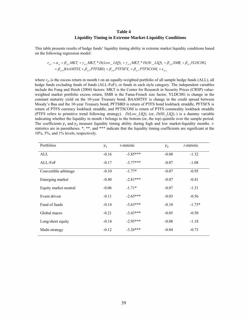
39

Table 4 Liquidity Timing in Extreme Market-Liquidity Conditions

This table presents results of hedge funds’ liquidity timing ability in extreme market liquidity conditions based on the following regression model:

,,7,6,5,4,

3,2,2,1,1,, )_(*)_(*

tptptptptp

tptpttpttptpptp

PTFSCOMPTFSFXPTFSBDBAAMTSYYLDCHGSMBLIQHiDMKTLIQLowDMKTMKTr

εββββ

ββγγβα

+++++

+++++=

where rpt is the excess return in month t on an equally-weighted portfolio of all sample hedge funds (ALL), all hedge funds excluding funds of funds (ALL-FoF), or funds in each style category. The independent variables include the Fung and Hsieh (2004) factors: MKT is the Center for Research in Security Prices (CRSP) value-weighted market portfolio excess return, SMB is the Fama-French size factor, YLDCHG is change in the constant maturity yield on the 10-year Treasury bond, BAAMTSY is change in the credit spread between Moody’s Baa and the 10-year Treasury bond, PFTSBD is return of PTFS bond lookback straddle, PFTSFX is return of PTFS currency lookback straddle, and PFTSCOM is return of PTFS commodity lookback straddle (PTFS refers to primitive trend following strategy). D(Low_LIQ)t (or, D(Hi_LIQ)t ) is a dummy variable indicating whether the liquidity in month t belongs to the bottom (or, the top) quintile over the sample period. The coefficients and measure liquidity timing ability during high and low market-liquidity months. t-statistics are in parentheses. *, **, and *** indicate that the liquidity timing coefficients are significant at the 10%, 5%, and 1% levels, respectively.

Portfolios t-statistic t-statistic

ALL -0.16 -3.85*** -0.08 -1.32

ALL-FoF -0.17 -3.77*** -0.07 -1.08

Convertible arbitrage -0.10 -1.77* -0.07 -0.95

Emerging market -0.40 -2.81*** -0.07 -0.41

Equity market neutral -0.06 -1.71* -0.07 -1.31

Event driven -0.11 -2.65*** -0.03 -0.56

Fund of funds -0.14 -3.63*** -0.10 -1.73*

Global macro -0.21 -3.43*** -0.05 -0.50

Long/short equity -0.14 -2.95*** -0.08 -1.18

Multi-strategy -0.12 -3.26*** -0.04 -0.73

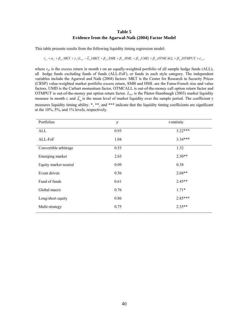
40

Table 5 Evidence from the Agarwal-Naik (2004) Factor Model

This table presents results from the following liquidity timing regression model:

,)( ,6,5,4,3,2,,1,, tptptptptptptmtmptpptp OTMPUTOTMCALLUMDHMLSMBMKTLLMKTr εβββββγβα ++++++−++= where rpt is the excess return in month t on an equally-weighted portfolio of all sample hedge funds (ALL), all hedge funds excluding funds of funds (ALL-FoF), or funds in each style category. The independent variables include the Agarwal and Naik (2004) factors: MKT is the Center for Research in Security Prices (CRSP) value-weighted market portfolio excess return, SMB and HML are the Fama-French size and value factors, UMD is the Carhart momentum factor, OTMCALL is out-of-the-money call option return factor and OTMPUT is out-of-the-money put option return factor. Lm,t is the Pástor-Stambaugh (2003) market liquidity measure in month t, and mL is the mean level of market liquidity over the sample period. The coefficient γ measures liquidity timing ability. *, **, and *** indicate that the liquidity timing coefficients are significant at the 10%, 5%, and 1% levels, respectively.

Portfolios γ t-statistic

ALL 0.93 3.22***

ALL-FoF 1.04 3.34***

Convertible arbitrage 0.53 1.32

Emerging market 2.63 2.30**

Equity market neutral 0.09 0.38

Event driven 0.56 2.04**

Fund of funds 0.61 2.45**

Global macro 0.76 1.71*

Long/short equity 0.86 2.85***

Multi-strategy 0.75 2.35**

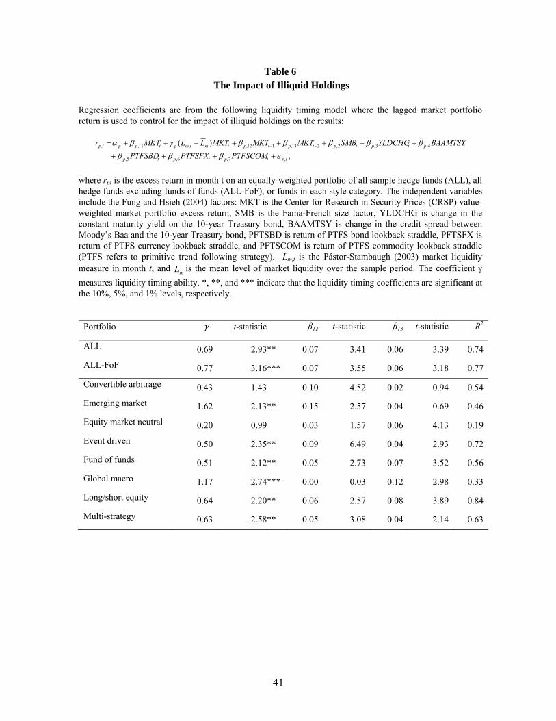
41

Table 6 The Impact of Illiquid Holdings

Regression coefficients are from the following liquidity timing model where the lagged market portfolio return is used to control for the impact of illiquid holdings on the results:

,)(

,7,6,5,

4,3,2,213,112,,11,,

tptptptp

tptptptptptmtmptpptp

PTFSCOMPTFSFXPTFSBDBAAMTSYYLDCHGSMBMKTMKTMKTLLMKTr

εβββ

βββββγβα

++++

+++++−++= −−

where rpt is the excess return in month t on an equally-weighted portfolio of all sample hedge funds (ALL), all hedge funds excluding funds of funds (ALL-FoF), or funds in each style category. The independent variables include the Fung and Hsieh (2004) factors: MKT is the Center for Research in Security Prices (CRSP) value-weighted market portfolio excess return, SMB is the Fama-French size factor, YLDCHG is change in the constant maturity yield on the 10-year Treasury bond, BAAMTSY is change in the credit spread between Moody’s Baa and the 10-year Treasury bond, PFTSBD is return of PTFS bond lookback straddle, PFTSFX is return of PTFS currency lookback straddle, and PFTSCOM is return of PTFS commodity lookback straddle (PTFS refers to primitive trend following strategy). Lm,t is the Pástor-Stambaugh (2003) market liquidity measure in month t, and mL is the mean level of market liquidity over the sample period. The coefficient γ measures liquidity timing ability. *, **, and *** indicate that the liquidity timing coefficients are significant at the 10%, 5%, and 1% levels, respectively.

Portfolio γ t-statistic β12 t-statistic β13 t-statistic R2

ALL 0.69 2.93** 0.07 3.41 0.06 3.39 0.74

ALL-FoF 0.77 3.16*** 0.07 3.55 0.06 3.18 0.77

Convertible arbitrage 0.43 1.43 0.10 4.52 0.02 0.94 0.54

Emerging market 1.62 2.13** 0.15 2.57 0.04 0.69 0.46

Equity market neutral 0.20 0.99 0.03 1.57 0.06 4.13 0.19

Event driven 0.50 2.35** 0.09 6.49 0.04 2.93 0.72

Fund of funds 0.51 2.12** 0.05 2.73 0.07 3.52 0.56

Global macro 1.17 2.74*** 0.00 0.03 0.12 2.98 0.33

Long/short equity 0.64 2.20** 0.06 2.57 0.08 3.89 0.84

Multi-strategy 0.63 2.58** 0.05 3.08 0.04 2.14 0.63

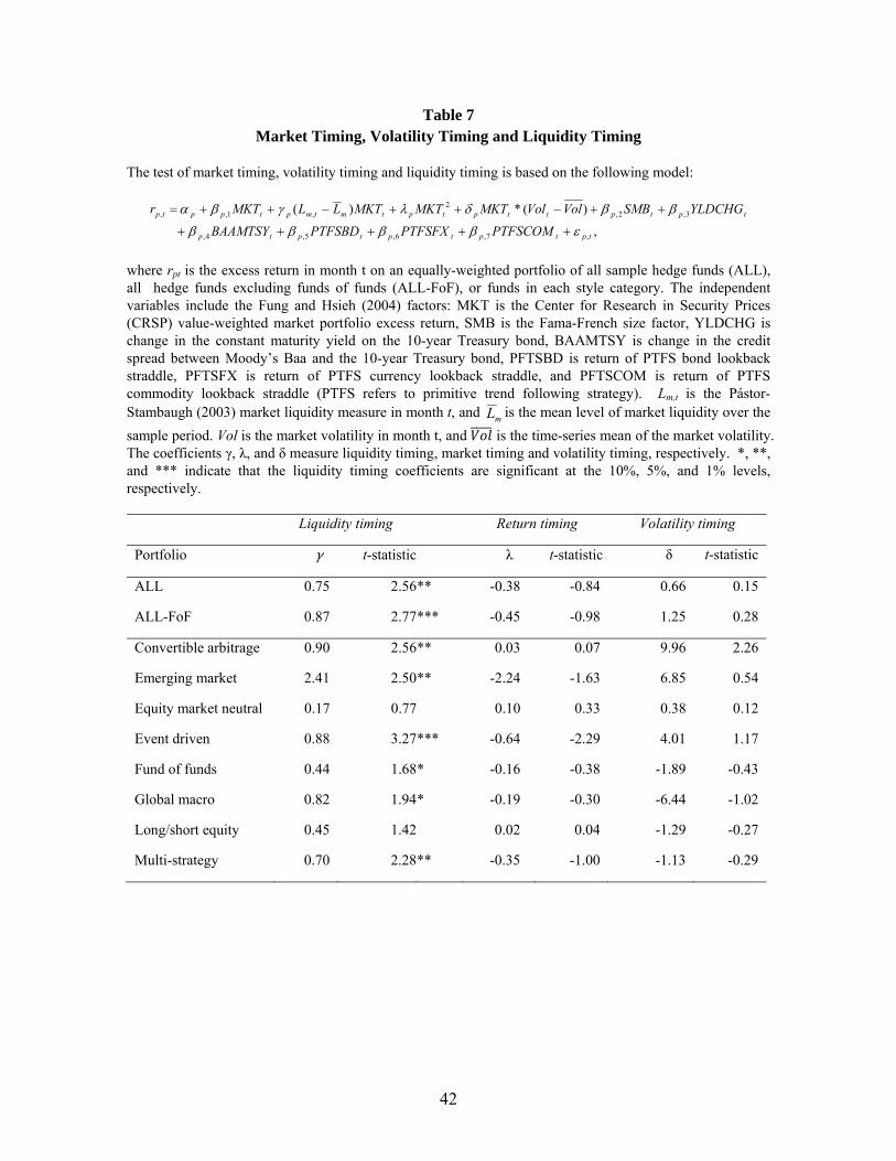
42

Table 7 Market Timing, Volatility Timing and Liquidity Timing

The test of market timing, volatility timing and liquidity timing is based on the following model:

,

)(*)(

,7,6,5,4,

3,2,2

,1,,

tptptptptp

tptpttptptmtmptpptp

PTFSCOMPTFSFXPTFSBDBAAMTSY

YLDCHGSMBVolVolMKTMKTMKTLLMKTr

εββββ

ββδλγβα

+++++

++−++−++=

where rpt is the excess return in month t on an equally-weighted portfolio of all sample hedge funds (ALL), all hedge funds excluding funds of funds (ALL-FoF), or funds in each style category. The independent variables include the Fung and Hsieh (2004) factors: MKT is the Center for Research in Security Prices (CRSP) value-weighted market portfolio excess return, SMB is the Fama-French size factor, YLDCHG is change in the constant maturity yield on the 10-year Treasury bond, BAAMTSY is change in the credit spread between Moody’s Baa and the 10-year Treasury bond, PFTSBD is return of PTFS bond lookback straddle, PFTSFX is return of PTFS currency lookback straddle, and PFTSCOM is return of PTFS commodity lookback straddle (PTFS refers to primitive trend following strategy). Lm,t is the Pástor-Stambaugh (2003) market liquidity measure in month t, and mL is the mean level of market liquidity over the sample period. Vol is the market volatility in month t, and is the time-series mean of the market volatility. The coefficients γ, λ, and δ measure liquidity timing, market timing and volatility timing, respectively. *, **, and *** indicate that the liquidity timing coefficients are significant at the 10%, 5%, and 1% levels, respectively.

Liquidity timing Return timing Volatility timing

Portfolio γ t-statistic λ t-statistic δ t-statistic

ALL 0.75 2.56** -0.38 -0.84 0.66 0.15

ALL-FoF 0.87 2.77*** -0.45 -0.98 1.25 0.28

Convertible arbitrage 0.90 2.56** 0.03 0.07 9.96 2.26

Emerging market 2.41 2.50** -2.24 -1.63 6.85 0.54

Equity market neutral 0.17 0.77 0.10 0.33 0.38 0.12

Event driven 0.88 3.27*** -0.64 -2.29 4.01 1.17

Fund of funds 0.44 1.68* -0.16 -0.38 -1.89 -0.43

Global macro 0.82 1.94* -0.19 -0.30 -6.44 -1.02

Long/short equity 0.45 1.42 0.02 0.04 -1.29 -0.27

Multi-strategy 0.70 2.28** -0.35 -1.00 -1.13 -0.29

43

Table 8 Liquidity Timing Ability: Evidence at the Fund Level

This table presents cross-sectional distribution of individual funds’ liquidity timing coefficients. For each fund with at least 24 monthly return observations, we estimate the following liquidity timing model:

,

)(

,7,6,5,

4,3,2,,1,,

tptptptp

tptptptmtmptpptp

PTFSCOMPTFSFXPTFSBD

BAAMTSYYLDCHGSMBMKTLLMKTr

εβββ

βββγβα

++++

+++−++=

where rit is the excess return on fund i in month t. The independent variables include the Fung and Hsieh (2004) factors: MKT is the Center for Research in Security Prices (CRSP) value-weighted market portfolio excess return, SMB is the Fama-French size factor, YLDCHG is change in the constant maturity yield on the 10-year Treasury bond, BAAMTSY is change in the credit spread between Moody’s Baa and the 10-year Treasury bond, PFTSBD is return of PTFS bond lookback straddle, PFTSFX is return of PTFS currency lookback straddle, and PFTSCOM is return of PTFS commodity lookback straddle (PTFS refers to primitive trend following strategy). Lm,t is the Pástor-Stambaugh (2003) market liquidity measure in month t, and mL is the mean level of market liquidity over the sample period. The coefficient γ measures liquidity timing ability.

# of funds

Bottom of γ coefficient Top of γ coefficient

% of t-statistic negative

and significant

at 5%

% of t-statistic positive

and significant

at 5% 5% 10% 15% 20% 20% 15% 10% 5%

All funds 2,358 -4.58 -2.89 -2.08 -1.61 1.10 1.42 2.05 3.29 14.72 13.99

All funds excluding Funds of Funds 1,706 -5.31 -3.28 -2.19 -1.66 1.37 1.74 2.53 3.78 13.77 13.54

Convertible arbitrage 75 -4.81 -2.16 -1.42 -1.00 0.55 0.70 0.91 2.65 9.33 12.00

Emerging market

171 -7.74 -4.58 -2.90 -1.98 2.52 2.82 5.10 6.92 12.28 16.37 Equity market neutral

133 -3.95 -2.83 -2.26 -1.71 0.58 0.81 1.20 1.46 15.04 3.76 Event driven

251 -3.26 -2.09 -1.65 -1.30 0.85 1.03 1.44 2.55 15.14 13.94 Fund of funds

652 -3.17 -2.31 -1.89 -1.49 0.65 0.81 1.05 1.35 17.18 15.18 Global macro

107 -5.49 -2.66 -1.92 -1.40 2.00 2.47 3.29 4.30 10.28 14.02 Long/short equity

789 -6.48 -3.97 -2.80 -1.93 1.57 2.08 2.79 3.83 13.43 15.46 Multi-strategy

175 -4.43 -2.84 -2.08 -1.67 0.77 1.00 1.41 2.17 17.14 9.71

44

Table 9 Bootstrap Analysis of Liquidity Timing

This table presents the evidence from a bootstrap analysis of liquidity timing ability of individual hedge funds. The first row reports the sorted t-statistic of liquidity timing coefficient across individual funds, while the second row is the empirical p-value from bootstrap simulations. The number of resampling iterations is 1,000.

Bottom t-statistic of γ coefficient Top t-statistic of γ coefficient # of funds 1% 3% 5% 10% 15% 20% 20% 15% 10% 5% 3% 1%

All funds 2,358 t-stat -3.66 -2.93 -2.59 -1.96 -1.58 -1.28 1.28 1.56 1.92 2.46 2.91 3.49

p-value 0.00 0.00 0.00 0.00 0.00 0.00 0.00 0.00 0.00 0.00 0.00 0.00 All funds excluding Funds of Funds

1,706 t-stat -3.63 -2.83 -2.50 -1.94 -1.51 -1.19 1.27 1.54 1.89 2.38 2.84 3.44 p-value 0.00 0.00 0.00 0.00 0.00 0.00 0.00 0.00 0.00 0.00 0.00 0.00

Convertible arbitrage 75 t-stat -3.75 -2.62 -2.34 -1.28 -1.13 -0.86 1.19 1.49 1.78 2.19 2.40 3.40

p-value 0.15 0.14 0.16 0.82 0.73 0.79 0.19 0.16 0.15 0.26 0.29 0.27 Emerging market

171 t-stat -3.93 -3.00 -2.31 -1.85 -1.49 -1.24 1.50 1.88 2.27 2.68 3.07 3.89 p-value 0.05 0.00 0.07 0.03 0.02 0.03 0.00 0.00 0.00 0.00 0.00 0.04

Equity market neutral 133 t-stat -2.94 -2.65 -2.31 -1.87 -1.64 -1.45 0.84 1.19 1.41 1.56 1.89 2.14

p-value 0.47 0.24 0.15 0.09 0.01 0.01 0.87 0.69 0.85 0.98 0.97 0.98 Event driven

251 t-stat -3.57 -2.83 -2.39 -1.94 -1.66 -1.08 1.27 1.52 2.02 2.63 2.83 3.16 p-value 0.06 0.01 0.02 0.00 0.00 0.22 0.01 0.01 0.00 0.00 0.01 0.26

Fund of funds 652 t-stat -3.66 -3.06 -2.75 -2.10 -1.73 -1.45 1.33 1.65 2.00 2.64 3.17 3.51

p-value 0.01 0.00 0.00 0.00 0.00 0.00 0.00 0.00 0.00 0.00 0.00 0.02 Global macro

107 t-stat -2.67 -2.63 -2.15 -1.65 -1.22 -0.87 1.33 1.58 1.81 2.11 2.18 2.61 p-value 0.62 0.18 0.50 0.37 0.62 0.84 0.05 0.04 0.12 0.52 0.63 0.65

Long/short equity 789 t-stat -3.63 -2.84 -2.47 -1.94 -1.49 -1.14 1.40 1.67 1.97 2.66 3.17 3.95

p-value 0.01 0.00 0.00 0.00 0.00 0.01 0.00 0.00 0.00 0.00 0.00 0.00 Multi-strategy

175 t-stat -4.98 -3.02 -2.80 -2.30 -1.99 -1.50 1.09 1.37 1.60 2.08 2.22 2.46 p-value 0.00 0.01 0.00 0.00 0.00 0.00 0.32 0.23 0.37 0.39 0.60 0.91

45

Table 10 Cross-Sectional Regression Analysis of Liquidity Timing Ability

This table reports the results from a cross-sectional regression, where the dependent variable is the liquidity timing coefficient for each sample fund and the independent variables include fund characteristics and category dummies. Minimum investment is the minimum required investment from an investor in millions of dollars; Management fee is in percent of assets under management; Incentive fee is in percentage of the profits; Redemption restriction period is the combination of lock-up period during which investors’ money is locked up and advanced notice period that is the time needed for investors to notify managers before they can withdraw money; Effective auditing dummy=1 if the fund provides both its auditor’s name and audit date and 0 otherwise; Leverage dummy=1 if the fund uses leverage and 0 otherwise; Personal capital dummy=1 if the fund manager invests own money in the fund and 0 otherwise. ** and *** indicate significance at the 5% and 1% levels, respectively. The number of funds in this test is 2,330. Variable Coefficient t-statistic

Constant -0.023 -0.11

Minimum investment ($million) -0.034 -0.39

Management fee -0.437 -5.20***

Incentive fee 0.003 0.59

Redemption restriction period (month) -0.004 -0.60

Effective auditing dummy 0.215 2.45**

Leverage dummy 0.205 3.16***

Personal capital dummy 0.233 3.38***

Category dummies Yes

Number of funds 2,330

Adjusted R2 0.041

46

Table 11 Investment Value of Liquidity Timing

This table presents investment value of liquidity timing ability. In each month since January 1997 we form 10 portfolios based on hedge funds’ liquidity timing coefficients in the past three years (i.e., estimation period is 36 months). Portfolios are held for different holding periods of K months, i.e., K=3, 6, 9, and 12 months. We report the Fung and Hsieh seven-factor alphas of the decile portfolios, the spread between top and bottom portfolio, and the spread between top portfolio and the equally-weighted portfolio of all funds. Alphas are in percent per month. t-statistics are in parentheses.

Portfolio Panel A: All Funds Panel B: All Funds Excluding FOFs

K=3 6 9 12 K=3 6 9 12 Portfolio 1 (top timers) 0.63 0.67 0.68 0.65 0.70 0.75 0.77 0.75

(3.67) (4.03) (4.14) (3.96) (3.55) (3.87) (4.00) (3.85)

Portfolio 2 0.46 0.46 0.46 0.46 0.40 0.43 0.45 0.48 (4.31) (4.41) (4.67) (4.70) (3.25) (3.77) (4.17) (4.43)

Portfolio 3 0.30 0.32 0.33 0.33 0.45 0.46 0.46 0.45 (3.18) (3.69) (3.85) (3.81) (4.88) (5.20) (5.38) (5.16)

Portfolio 4 0.35 0.33 0.32 0.30 0.32 0.31 0.30 0.30 (4.14) (3.91) (3.84) (3.67) (3.31) (3.60) (3.71) (3.70)

Portfolio 5 0.28 0.30 0.30 0.30 0.37 0.38 0.37 0.35 (3.22) (3.54) (3.58) (3.63) (4.58) (4.85) (4.87) (4.83)

Portfolio 6 0.26 0.26 0.27 0.27 0.30 0.28 0.28 0.28 (3.07) (3.00) (3.18) (3.22) (3.86) (3.50) (3.57) (3.59)

Portfolio 7 0.24 0.27 0.27 0.28 0.22 0.26 0.27 0.29 (2.51) (2.82) (2.89) (2.96) (2.08) (2.57) (2.82) (3.03)

Portfolio 8 0.27 0.25 0.26 0.27 0.33 0.30 0.27 0.28 (2.83) (2.76) (2.78) (2.88) (3.06) (2.79) (2.57) (2.73)

Portfolio 9 0.27 0.23 0.23 0.26 0.23 0.23 0.28 0.30 (2.64) (2.19) (2.17) (2.52) (2.17) (2.04) (2.42) (2.71)

Portfolio 10 (bottom timers) 0.24 0.23 0.19 0.19 0.37 0.31 0.22 0.20 (1.44) (1.43) (1.19) (1.19) (2.00) (1.68) (1.21) (1.11)

Spread (1-10) 0.39 0.44 0.49 0.46 0.33 0.44 0.55 0.55

(2.18) (2.60) (3.04) (3.06) (1.55) (2.18) (2.80) (2.90)

Spread between Portfolio 1 0.23 0.27 0.28 0.25 0.25 0.29 0.32 0.29 and EWP of all funds (2.02) (2.38) (2.51) (2.35) (1.79) (2.11) (2.28) (2.16)

47

Table A.1 Reaction to Past Liquidity Conditions: Portfolio-Level Evidence

This table presents results from the following regression model:

,)( ,7,6,5,4,3,2,1,1,, tptptptptptptptmtmptpptp PTFSCOMPTFSFXPTFSBDBAAMTSYYLDCHGSMBMKTLLMKTr εββββββθβα +++++++−++= −

where rpt is the excess return in month t on an equally-weighted portfolio of all sample hedge funds (ALL), all hedge funds excluding funds of funds (ALL-FoF), or funds in each style category. The independent variables include the Fung and Hsieh (2004) factors: MKT is the Center for Research in Security Prices (CRSP) value-weighted market portfolio excess return, SMB is the Fama-French size factor, YLDCHG is change in the constant maturity yield on the 10-year Treasury bond, BAAMTSY is change in the credit spread between Moody’s Baa and the 10-year Treasury bond, PFTSBD is return of PTFS bond lookback straddle, PFTSFX is return of PTFS currency lookback straddle, and PFTSCOM is return of PTFS commodity lookback straddle (PTFS refers to primitive trend following strategy). Lm,t-1 is the Pástor-Stambaugh (2003) market liquidity measure in month t-1, and mL is the mean level of market liquidity over the sample period. The coefficient θ measures reaction to past liquidity conditions. t-statistics are in parentheses. *, **, and *** indicate that the liquidity reaction coefficients (θ) are significant at the 10%, 5%, and 1% levels, respectively.

48

Table A.1 (continued)

Portfolio             α β1 θ β2 β3 β4 β5x100 β6x100 β7x100 R2

ALL 0.42 0.32 0.87 0.15 1.17 -1.46 -1.50 0.79 0.72 0.71 (5.42) (11.70) (3.31)*** (4.86) (1.71) (-1.93) (-2.19) (1.83) (1.17) ALL-FoF 0.48 0.37 0.81 0.16 1.17 -1.26 -1.74 0.73 0.43 0.74 (6.02) (12.40) (2.96)*** (4.88) (1.69) (-1.68) (-2.32) (1.65) (0.67)

Convertible arbitrage 0.26 0.16 0.02 0.08 3.12 -4.07 -1.69 -0.02 -0.09 0.48 (2.75) (5.07) (0.07) (2.50) (3.43) (-3.42) (-2.09) (-0.04) (-0.14) Emerging market 0.50 0.56 1.00 0.22 4.18 -2.65 -5.35 0.14 0.30 0.44 (1.88) (6.01) (1.17) (2.71) (2.31) (-1.59) (-2.01) (0.11) (0.15) Equity market neutral 0.59 0.08 0.44 0.03 0.03 -0.90 -0.67 0.47 0.41 0.15 (8.21) (4.14) (2.18)** (1.95) (0.05) (-1.65) (-1.40) (1.33) (0.77) Event driven 0.50 0.18 0.36 0.08 1.96 -2.52 -1.75 0.53 0.00 0.62 (7.56) (7.44) (1.57) (3.34) (3.53) (-3.89) (-3.13) (1.57) (0.00) Fund of funds 0.26 0.20 1.07 0.11 1.19 -2.06 -0.90 0.93 1.54 0.53 (3.35) (8.14) (3.63)*** (4.49) (1.72) (-2.54) (-1.51) (2.14) (2.54) Global macro 0.48 0.22 1.53 0.06 -0.64 -1.35 -1.25 3.09 2.19 0.31 (3.67) (5.24) (2.59)** (1.52) (-0.77) (-1.81) (-1.19) (3.28) (1.86) Long short equity 0.54 0.48 0.96 0.21 0.45 -0.50 -0.85 0.76 0.41 0.82 (6.97) (18.50) (3.41)*** (6.17) (0.64) (-0.59) (-1.56) (1.64) (0.67) Multi-strategy 0.44 0.23 0.63 0.08 1.25 -1.69 -0.71 0.26 0.59 0.60 (6.46) (8.78) (2.64)*** (2.70) (1.86) (-2.40) (-1.10) (0.78) (1.11)

49

Table A.2 Reaction to Past Liquidity Conditions: Evidence at the Fund Level

This table presents cross-sectional distribution of individual funds’ reactions to past liquidity conditions. For each fund with at least 24 monthly return observations, we estimate the following regression model:

,

)(

,7,6,5,

4,3,2,1,1,,

tptptptp

tptptptmtmptpptp

PTFSCOMPTFSFXPTFSBD

BAAMTSYYLDCHGSMBMKTLLMKTr

εβββ

βββθβα

++++

+++−++= −

where rit is the excess return on fund i in month t. The independent variables include the Fung and Hsieh (2004) factors: MKT is the Center for Research in Security Prices (CRSP) value-weighted market portfolio excess return, SMB is the Fama-French size factor, YLDCHG is change in the constant maturity yield on the 10-year Treasury bond, BAAMTSY is change in the credit spread between Moody’s Baa and the 10-year Treasury bond, PFTSBD is return of PTFS bond lookback straddle, PFTSFX is return of PTFS currency lookback straddle, and PFTSCOM is return of PTFS commodity lookback straddle (PTFS refers to primitive trend following strategy). Lm,t-1 is the Pástor-Stambaugh (2003) market liquidity measure in month t-1, and

mL is the mean level of market liquidity over the sample period. The coefficient θ measures reaction to past liquidity conditions.

# of funds

Bottom of θ  coefficient Top of θ  coefficient % of

t-statistic negative

and significant

at 5%

% of t-statistic positive

and significant

at 5% 5% 10% 15% 20% 20% 15% 10% 5%

All funds 2358 -1.94 -0.84 -0.28 -0.04 2.81 3.26 4.11 5.75 3.10 38.63

All funds excluding Funds of Funds 1706 -2.36 -1.15 -0.60 -0.26 2.77 3.22 4.22 6.09 4.10 28.78

Convertible arbitrage 75 -2.47 -1.56 -1.39 -1.13 1.80 2.27 3.32 4.41 10.67 17.33

Emerging market 171 -1.18 -0.35 -0.09 0.04 4.23 4.88 5.98 7.86 0.58 31.58

Equity market neutral 133 -2.77 -1.17 -0.84 -0.42 1.64 2.39 2.90 3.72 6.77 24.81

Event driven 251 -1.16 -0.48 -0.29 -0.13 1.98 2.28 2.55 3.99 2.79 26.69

Fund of funds 652 -0.17 0.22 0.39 0.51 2.92 3.35 3.96 5.23 0.46 64.42

Global macro 107 -4.13 -2.02 -1.32 -0.73 4.91 5.51 6.60 8.55 6.54 28.97

Long short equity 789 -3.09 -1.41 -0.85 -0.27 2.89 3.31 4.14 6.21 3.68 29.53

Multi-strategy 175 -2.01 -0.74 -0.47 -0.16 2.89 3.38 4.34 5.50 5.14 33.71

50

Table A.3 Bootstrap Analysis of Liquidity Reaction

This table presents the evidence from a bootstrap analysis of liquidity reaction of individual hedge funds. The first row reports the sorted t-statistic of liquidity reaction coefficient across individual funds, while the second row is the empirical p-value from bootstrap simulations. The number of resampling iterations is 1,000.

Bottom t-statistic of θ  coefficient Top t-statistic of θ coefficient # of funds 1% 3% 5% 10% 15% 20% 20% 15% 10% 5% 3% 1%

All funds 2358 t-stat -2.48 -1.66 -1.26 -0.69 -0.31 -0.05 2.40 2.70 3.07 3.61 3.95 4.72

p-value 1.00 1.00 1.00 1.00 1.00 1.00 0.00 0.00 0.00 0.00 0.00 0.00 All funds excluding Funds of Funds

1706 t-stat -2.67 -1.80 -1.47 -0.88 -0.52 -0.27 1.99 2.26 2.61 3.13 3.48 4.02 p-value 1.00 1.00 1.00 1.00 1.00 1.00 0.00 0.00 0.00 0.00 0.00 0.00

Convertible arbitrage 75 t-stat -3.58 -2.03 -1.86 -1.65 -1.43 -1.29 1.37 1.85 2.19 2.89 2.99 3.52

p-value 0.25 0.69 0.69 0.31 0.24 0.11 0.04 0.01 0.00 0.01 0.04 0.26 Emerging market

171 t-stat -1.63 -1.15 -0.95 -0.36 -0.15 0.04 2.05 2.20 2.70 3.26 3.73 4.58 p-value 1.00 1.00 1.00 1.00 1.00 1.00 0.00 0.00 0.00 0.00 0.00 0.01

Equity market neutral 133 t-stat -2.59 -2.08 -1.75 -1.11 -0.59 -0.39 1.83 2.11 2.49 3.07 3.36 3.84

p-value 0.83 0.91 0.92 1.00 1.00 1.00 0.00 0.00 0.00 0.00 0.02 0.09 Event driven

251 t-stat -2.67 -1.30 -1.11 -0.64 -0.33 -0.21 2.00 2.14 2.49 3.10 3.32 4.12 p-value 0.84 1.00 1.00 1.00 1.00 1.00 0.00 0.00 0.00 0.00 0.00 0.01

Fund of funds 652 t-stat -1.30 -0.63 -0.15 0.34 0.76 1.02 3.10 3.42 3.72 4.28 4.72 5.77

p-value 1.00 1.00 1.00 1.00 1.00 1.00 0.00 0.00 0.00 0.00 0.00 0.00 Global macro

107 t-stat -2.86 -2.17 -2.13 -1.08 -0.75 -0.46 2.26 2.84 3.09 3.91 3.95 4.24 p-value 0.52 0.71 0.58 1.00 1.00 1.00 0.00 0.00 0.00 0.00 0.00 0.01

Long/short equity 789 t-stat -2.68 -1.71 -1.47 -0.83 -0.52 -0.24 1.99 2.27 2.58 3.12 3.33 3.89

p-value 0.98 1.00 1.00 1.00 1.00 1.00 0.00 0.00 0.00 0.00 0.00 0.00 Multi-strategy

175 t-stat -2.63 -1.81 -1.70 -1.00 -0.48 -0.25 2.18 2.51 2.94 3.74 3.85 4.31 p-value 0.88 0.99 0.96 1.00 1.00 1.00 0.00 0.00 0.00 0.00 0.00 0.04

51

Table A.4 Investment Value of Liquidity Reaction

This table presents investment value of liquidity reaction. In each month since January 1997 we form 10 portfolios based on hedge funds’ liquidity reaction coefficients in the past three years (i.e., estimation period is 36 months). Portfolios are held for different holding periods of K months, i.e., K=3, 6, 9, and 12 months. We report the Fung and Hsieh seven-factor alphas of the decile portfolios, the spread between top and bottom portfolio, and the spread between top portfolio and the equally-weighted portfolio of all funds. Alphas are in percent per month. t-statistics are in parentheses.

Portfolio Panel A: All Funds Panel B: All Funds Excluding FOFs

K=3 6 9 12 K=3 6 9 12 Portfolio 1 (top reactors) 0.32 0.32 0.35 0.37 0.36 0.36 0.36 0.37

(1.75) (1.79) (2.03) (2.22) (1.83) (1.82) (1.89) (1.94)

Portfolio 2 0.39 0.39 0.38 0.39 0.38 0.41 0.43 0.43 (2.76) (2.93) (2.96) (3.07) (2.48) (2.79) (3.19) (3.35)

Portfolio 3 0.30 0.27 0.27 0.27 0.37 0.34 0.31 0.32 (3.04) (2.87) (2.79) (2.82) (3.27) (3.30) (2.95) (3.26)

Portfolio 4 0.34 0.31 0.28 0.28 0.29 0.27 0.28 0.29 (3.72) (3.35) (3.14) (3.10) (3.16) (3.15) (3.35) (3.48)

Portfolio 5 0.25 0.24 0.25 0.25 0.25 0.23 0.25 0.26 (3.21) (3.09) (3.24) (3.26) (3.43) (3.20) (3.51) (3.49)

Portfolio 6 0.22 0.23 0.26 0.27 0.34 0.32 0.33 0.32 (2.84) (2.97) (3.34) (3.37) (4.56) (4.24) (4.24) (4.17)

Portfolio 7 0.28 0.30 0.29 0.28 0.38 0.40 0.41 0.39 (3.23) (3.45) (3.34) (3.12) (4.29) (4.62) (4.62) (4.40)

Portfolio 8 0.31 0.34 0.34 0.34 0.35 0.38 0.37 0.35 (3.65) (4.09) (4.11) (4.00) (3.72) (4.18) (4.17) (3.93)

Portfolio 9 0.35 0.38 0.35 0.35 0.36 0.38 0.35 0.35 (3.55) (3.96) (3.66) (3.74) (3.39) (3.52) (3.25) (3.09)

Portfolio 10 (bottom reactors) 0.56 0.55 0.54 0.55 0.59 0.57 0.59 0.60 (3.96) (3.87) (3.92) (3.97) (3.75) (3.75) (3.85) (3.95)

Spread (1-10) -0.24 -0.23 -0.19 -0.18 -0.22 -0.21 -0.23 -0.23

(-1.35) (-1.40) (-1.24) (-1.14) (-1.10) (-1.15) (-1.23) (-1.29)

Spread between Portfolio 1 -0.08 -0.08 -0.05 -0.03 -0.09 -0.09 -0.09 -0.08 and EWP of all funds (-0.66) (-0.70) (-0.45) (-0.23) (-0.65) (-0.74) (-0.72) (-0.70)