Can Nutritional Label Use Influence Dietary and Body

Weight Outcomes?

Rodolfo M. Nayga, Jr.

Professor and Tyson Endowed Chair

University of Arkansas

(work with Andreas Drichoutis and Panagiotis Lazaridis)

Introduction

Obesity rates have reached epidemic proportions in the US and many other countries.

• Several forms of cancer• Cardiovascular disease• Stroke• Social stigmatization• Depression• Low self esteem

• Osteoarthritis• Sleep apnea•Asthma•High blood pressure• Gallbladder disease• Cholesterol• Type II diabetes

In the US obesity approaches tobacco as top preventable cause of death

Determinants of obesity: An economic view

Obesity and Economic Costs

Economic impacts on health care systems (medical costs)

Direct Indirect

Preventive, diagnostic, treatment services

Morbidity costs: the value of income lost from decreased productivity, restricted activity, absenteeism, and sick bed days

Mortality costs: the value of future income lost by premature death

Obesity and Economic Costs

•Australia, Canada, England, France, New Zealand and USA: obesity accounts between 1%-8% of national health expenditures.

• In USA health care costs associated with obesity top $100 billion annually.

•World Bank estimates that 12% of the US national health care budget is spent treating obesity.

• 7% of healthcare costs in EU, are linked to obesity and related illnesses

Tackling the problem

Healthy diets and healthier food choices are becoming the target of many public programs and policies.

e.g.

US : Nutritional Labeling and Educational Act

NLEA• update list of nutrient, ingredients

• standardize serving sizes

• define nutrient content claims

• define health claims

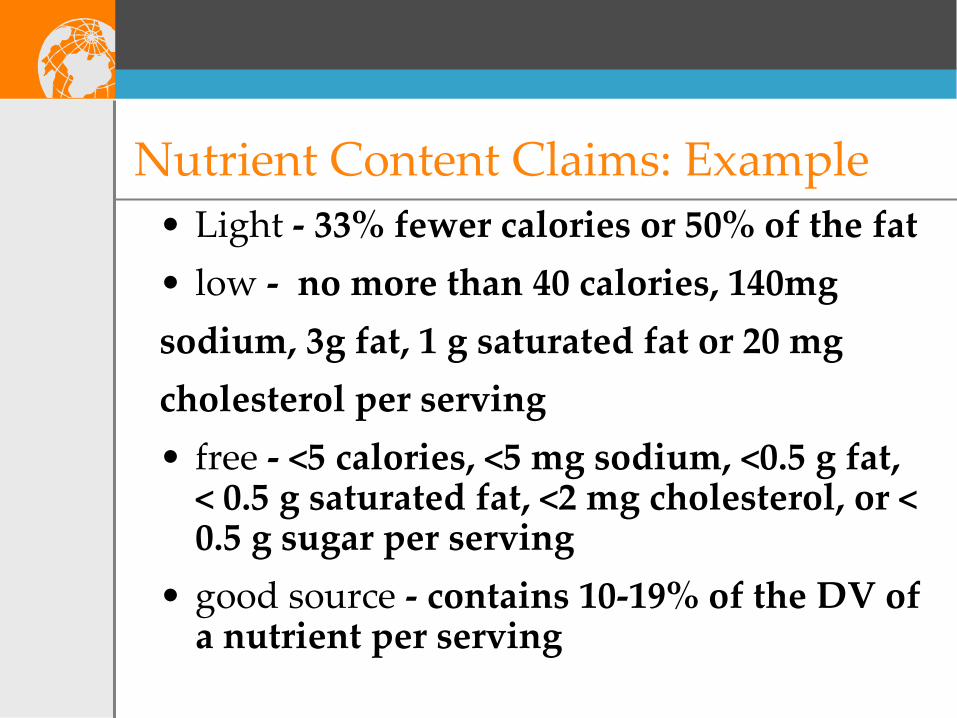
Nutrient Content Claims: Example• Light - 33% fewer calories or 50% of the fat• low - no more than 40 calories, 140mg sodium, 3g fat, 1 g saturated fat or 20 mg cholesterol per serving• free - <5 calories, <5 mg sodium, <0.5 g fat,

< 0.5 g saturated fat, <2 mg cholesterol, or <0.5 g sugar per serving

• good source - contains 10-19% of the DV of a nutrient per serving

Aims of NLEA• promote consumer nutritional education

• enable consumers to make more healthful food choices

• provide incentive to agri-food industry to create innovative and healthier new products for consumers

Tackling the problem

Previous studies have evaluated effect of nutritional label use

on dietary outcomes – generally found positive outcomes but magnitudes small!

•Coulson (2000)

•Guthrie et al. (1995)

•Russo et al. (1986)

•Kim, Nayga, and Capps (2000, 2001)

•Variyam (2004, 2008)

% Individuals Meeting the Dietary Guidelines: Calories from Total Fat

Calories from Total Fat

Non-Label Users

Label Users

Difference

30% or less 0.15 2.31 2.16

31-45% 70.56 97.69 27.13

>45% 29.29 0.00 -29.29

% Individuals Meeting the Dietary Guidelines: Calories from Saturated Fat

Calories from Saturated Fat

Non-Label Users

Label Users

Difference

<10% 0.29 8.82 8.53

10-15% 83.21 91.13 7.92

>15% 16.50 0.05 -16.45

• Assumption by policy-makers: nutritional labels can help reduce obesity rates?

• With the Health Care Reform Bill – nutritional labeling for restaurant chains

• Our research question: Can nutritional label use really influence body weight (Body Mass Index)?

Propensity score matching

Issue with IV - instruments

Matching methods represent either a semi-parametric or non-parametric alternative to linear regression

The propensity score was introduced by Rosenbaum and Rubin (1983) to provide an alternative method for estimating treatment effects when treatment assignment is not random.

Standard case: Binary treatment

Extensions: Multiple treatments

Propensity score matching: the binary treatment

The evaluation question• Question which we want to answer is (counterfactual question): “What would have happened to those who, in fact, did receive treatment, if they had not received treatment (or the converse)?”

•Problem is that it is impossible to observe both outcomes of interest to get the true causal effect

•Randomized experiment – requires lots of money and effort

•PSM mimics a randomized experiment (like a quasi-experiment)

PSM

• Idea – find a group of non-treated individuals that are similar to the treated individuals in all characteristics X

• Construct matching groups for label and non-label users

Propensity score matching: the binary treatment

Formally, assume that there is a variable Ti indicating treatment, which equals 1 if individual i uses nutritional labels (treated case) and 0 if individual i does not use nutritional labels (control case).

Propensity score - the conditional probability of receiving a treatment (using nutritional labels) given pre-treatment (not using nutritional labels) characteristics X:

( ) ( ) ( )Pr 1| |p X T X E T X≡ = =

Propensity score matching: the binary treatment

Conditional Independence Assumption (CIA) –

-assume that we have conditioned on all variables that influence both participation and outcome

- selection is solely based on observable characteristics

Propensity score matching: the binary treatment

Step by step:

1. Estimate binary probits (or logit).

2. Match based on propensity scores (probabilities).

3. Estimate the differences of the outcomes from the matched samples.

How about for multiple treatment levels?

Estimate a series of binomial models (Lechner, 2002, RES)

The data

National Health and Nutrition Examination Survey Scope: Assess health and nutritional status of people in the US, combines interviews and physical examinations

Interview: demographic, socioeconomic, dietary, health-related

Examination: medical, dental, physiological, laboratory testsmeasures how often consumers’ read Nutrition Fact Panels on a five likert scale (never, rarely, sometimes, most of the time, always)

The data

BMI – measured, not self-reported

Label use – (1) never, (2) rarely, (3) sometimes, (4) most of the time, (5) always read nutrition facts panel

X vector uses variables that we group in five categories:

a) Socio-demographic: age, gender, race, education, household size, income

b) Risky behavior: alcohol consumption, drug use, smoking status, safe sexual behavior

c) Lifestyle: FAFH consumption, exercise frequency, perceived healthfulness of diet, households’ food security

d) Knowledge: doctors advice (reduce weight, eat less fat), perceived knowledge of DG, FGP, 5aD and self-efficacy (some people are born to be fat; nothing you can do to change this)

e) Health situation: Pregnancy, diabetes, intake of diabetic medicine and chronic diseases status

Estimations: Plausibility of CIA

Have we conditioned on all variables that simultaneously influence participation decision and outcome?

There is no test!

We can only argue that: Given that we have an extremely rich and informative dataset that allows us to control for a wide variety of socio-demographic variables, risky behavior, lifestyle, knowledge and current health situation, we argue that the CIA holds.

Estimations: The matching procedure

We implement six matching algorithms:• One-to-one nearest neighbor• Spline smoothing• Local linear• Kernel• Radius matching with calipers (0.1, 0.01)

Use of the difference of the mean outcomes of the matched samples will yield the average treatment effect on the treated (ATT).

Computation of standard errors is not straightforward because the estimation steps that precede the matching process add variation. BOOTSTRAP variance estimator

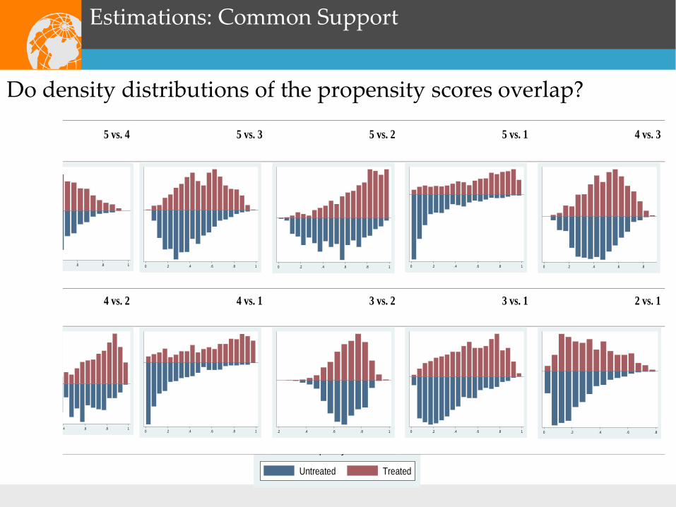
Estimations: Common Support

Do density distributions of the propensity scores overlap?

5 vs. 4 5 vs. 3 5 vs. 2 5 vs. 1 4 vs. 3

.6 .8 1 0 .2 .4 .6 .8 1 0 .2 .4 .6 .8 1 0 .2 .4 .6 .8 1 0 .2 .4 .6 .8

4 vs. 2 4 vs. 1 3 vs. 2 3 vs. 1 2 vs. 1

.4 .6 .8 1 0 .2 .4 .6 .8 1 .2 .4 .6 .8 1 0 .2 .4 .6 .8 1 0 .2 .4 .6 .8 p y

Untreated Treated

Participants Nonparticipants

Predicted Probability

Range of matched cases.

Cases excluded

Estimations: Common Support

Impose common support by “minima and maxima comparison”: DELETE observations whose propensity score is smaller than the minimum and larger than the maximum in the opposite group.

Before After % Lost Probability scoresModels Matching Min Max5 vs. 4 1550 1544 0.39 0.155 0.9005 vs. 3 1704 1698 0.35 0.056 0.9325 vs. 2 1163 1144 1.63 0.031 0.9845 vs. 1 2125 2122 0.14 0.006 0.9864 vs. 3 1790 1781 0.50 0.076 0.8144 vs. 2 1249 1209 3.20 0.057 0.9604 vs. 1 2211 2168 1.94 0.003 0.9653 vs. 2 1403 1399 0.29 0.328 0.9463 vs. 1 2365 2335 1.27 0.021 0.9172 vs. 1 1824 1823 0.05 0.008 0.772

Estimations: Results

5 vs. 1 4 vs. 1 3 vs. 1 2 vs. 1ATT diff.(S.E.)

ATT diff.(S.E.)

ATT diff.(S.E.)

ATT diff.(S.E.)

Unmatched 0.933**(0.323)

0.725**(0.306)

0.933**(0.289)

0.701*(0.387)

One-to-One nearest neighbor 0.127(0.647)

0.596(0.537)

0.952**(0.472)

-0.041(0.687)

Local linear regression 0.661(0.657)

0.642(0.505)

0.805**(0.367)

0.712*(0.429)

Spline-smoothing 0.671(0.556)

0.671(0.503)

0.785**(0.359)

0.648*(0.385)

Kernel (epanechnikov) 0.662(0.642)

0.617(0.466)

0.774**(0.356)

0.669(0.431)

Radius, Caliper=0.1 0.654(0.600)

0.676(0.437)

0.803**(0.359)

0.680*(0.402)

Radius, Caliper=0.01 0.434(0.642)

0.673(0.472)

0.774**(0.372)

0.818*(0.431)

Estimations: Robustness check

We used another much older dataset: Continuing Survey of Food Intakes for Individuals (CSFII)

- Same results!

Estimations: Robustness checks

4 vs. 1 3 vs. 1 2 vs. 1ATT diff.(S.E.)

ATT diff.(S.E.)

ATT diff.(S.E.)

Unmatched 0.934 (0.467)**

0.301 (0.409)

0.066 (0.511)

One-to-One nearest neighbor

0.746 (0.844)

0.706 (0.648)

0.794 (0.658)

Local linear regression 0.956 (0.826)

0.395 (0.658)

0.499 (0.512)

Spline-smoothing 1.047 (0.782)

0.497 (0.595)

0.410 (0.491)

Kernel (epanechnikov) 0.922 (0.786)

0.477 (0.657)

0.491 (0.511)

Radius, Caliper=0.1 0.987 (0.798)

0.719 (0.525)

0.441 (0.500)

Radius, Caliper=0.01 0.961 (0.690)

0.603 (0.524)

0.578 (0.489)

Sensitivity Analysis for Unobserved Heterogeneity

Rosenbaum bounds - assess sensitivity of significance levels of treatment effects- assumes that participation probability is not only determined by observable but also unobservable component

u

- If no hidden bias, is zero- varying this value allows us to assess sensitivity of results to hidden bias - results suggest label use unlikely to have an effect on BMI

even in presence of unobserved heterogeneity

( ) ( )Pr 1|i i i i iT X F X uπ β γ= = = +

γ

Conclusions

Policy relevant question: Can nutritional label use reduce body weight?

Answer: NO! Not yet anyway based on our study.