can subnetwork structure be the key to out-of-distribution

Can Subnetwork Structure be the Key to Out-of-Distribution Generalization?

Dinghuai Zhang 1 Kartik Ahuja 1 Yilun Xu 2 Yisen Wang 3 Aaron Courville 1

Abstract

Can models with particular structure avoid be-ing biased towards spurious correlation in out-of-distribution (OOD) generalization? Peters et al.(2016) provides a positive answer for linear cases.In this paper, we use a functional modular prob-ing method to analyze deep model structures un-der OOD setting. We demonstrate that even inbiased models (which focus on spurious correla-tion) there still exist unbiased functional subnet-works. Furthermore, we articulate and demon-strate the functional lottery ticket hypothesis: fullnetwork contains a subnetwork that can achievebetter OOD performance. We then propose Mod-ular Risk Minimization to solve the subnetworkselection problem. Our algorithm learns the sub-network structure from a given dataset, and canbe combined with any other OOD regularizationmethods. Experiments on various OOD general-ization tasks corroborate the effectiveness of ourmethod.

1. IntroductionDespite the remarkable progress we have witnessed inneural-network-based machine learning, the stories of fail-ures continue to accumulate (Geirhos et al., 2020). Manyof these failures are attributed to models exploiting spuri-ous correlations or shortcuts (i.e. factors that are not usedto generate the label). A colloquial example comes from(Beery et al., 2018) where the authors show how a neuralnetwork trained to distinguish cows from camels exploitsshortcut such as background color for prediction. In a muchmore concerning example, (DeGrave et al., 2020) show howmachine learning systems trained to detect COVID-19 ex-ploited the data source (e.g., hospital) to artificially boostinference performance.

1Mila - Quebec AI Institute 2CSAIL, Massachusetts Instituteof Technology 3Key Lab of Machine Perception (MoE), School ofEECS, Peking University. Correspondence to: Dinghuai Zhang<[email protected]>.

Proceedings of the 38 th International Conference on MachineLearning, PMLR 139, 2021. Copyright 2021 by the author(s).

step

10

20

30

40

50

60

70

accu

racy

StructureFull networkRandlayer

Randwhole

MRM (Ours)Oracle

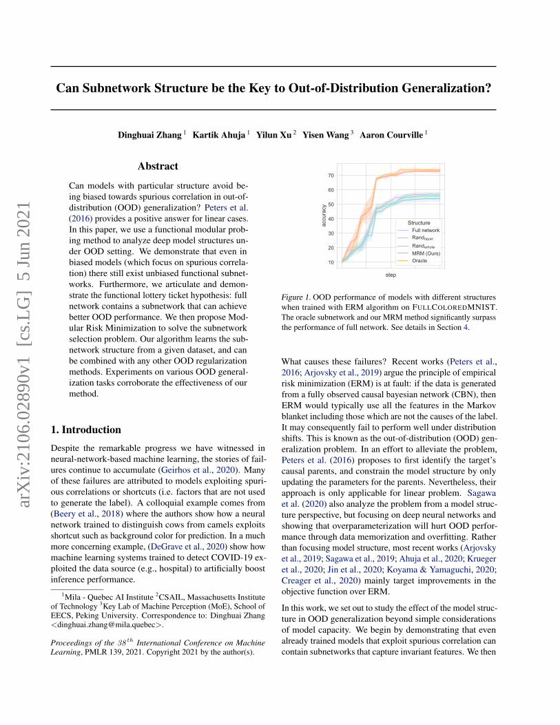
Figure 1. OOD performance of models with different structureswhen trained with ERM algorithm on FULLCOLOREDMNIST.The oracle subnetwork and our MRM method significantly surpassthe performance of full network. See details in Section 4.

What causes these failures? Recent works (Peters et al.,2016; Arjovsky et al., 2019) argue the principle of empiricalrisk minimization (ERM) is at fault: if the data is generatedfrom a fully observed causal bayesian network (CBN), thenERM would typically use all the features in the Markovblanket including those which are not the causes of the label.It may consequently fail to perform well under distributionshifts. This is known as the out-of-distribution (OOD) gen-eralization problem. In an effort to alleviate the problem,Peters et al. (2016) proposes to first identify the target’scausal parents, and constrain the model structure by onlyupdating the parameters for the parents. Nevertheless, theirapproach is only applicable for linear problem. Sagawaet al. (2020) also analyze the problem from a model struc-ture perspective, but focusing on deep neural networks andshowing that overparameterization will hurt OOD perfor-mance through data memorization and overfitting. Ratherthan focusing model structure, most recent works (Arjovskyet al., 2019; Sagawa et al., 2019; Ahuja et al., 2020; Kruegeret al., 2020; Jin et al., 2020; Koyama & Yamaguchi, 2020;Creager et al., 2020) mainly target improvements in theobjective function over ERM.

In this work, we set out to study the effect of the model struc-ture in OOD generalization beyond simple considerationsof model capacity. We begin by demonstrating that evenalready trained models that exploit spurious correlation cancontain subnetworks that capture invariant features. We then

arX

iv:2

106.

0289

0v1

[cs

.LG

] 5

Jun

202

1


turn to investigate whether the choice of structure mattersin the training process. To this end, we propose a functionallottery ticket hypothesis – a full network contains a subnet-work that can possibly achieve better performance for OODgeneralization than full network. We confirm this hypothe-sis by experiments on a manually crafted dataset (Figure 1)with our “oracle” subnetwork that uses information fromOOD examples. As a practical method to that avoids the useof OOD information, we propose the Modular Risk Min-imization (MRM) approach. MRM is a simple algorithmto address OOD tasks via structure learning. Our approachhunts for subnetworks with a better OOD inductive biasand can also combine with other OOD algorithms, bringingconsistent performance improvement. We summarize ourcontributions as follows:

• We show that large trained networks that exploit spu-rious correlations contain subnetworks that are lesssusceptible to these spurious shortcuts.

• We propose a novel functional lottery ticket hypothesis:there exists a subnetwork that can achieve better OODand commensurate in-distribution accuracy in a com-parable number of iterations when trained in isolation.

• We propose Modular Risk Minimization (MRM), astraightforward and effective algorithm to improveOOD generalization. MRM helps select subnetworksand can be used in conjunction with other methods(e.g., IRM) and boosts their performance as well.

2. Invariant Prediction2.1. Out-of-distribution (OOD) generalization problem

Consider a supervised learning setting where the data isgathered from different environments and each environ-ment represents a different probability distribution. Let(Xe, Y e) ∼ Pe, where Xe ∈ X , Y e ∈ Y stands forthe feature random variable and the corresponding label,e ∈ E = {1, ...,E} is the index for environments, and the setE corresponds to all possible environments. The set E isdivided into two sets: seen environments Eseen and unseenones Eunseen (E = Eseen ∪ Eunseen). The training dataset com-prises samples from Eseen. The dataset from environment eis given as De = {xei , yei }n

e

e=1, where each point (xei , yei ) isan independently identically distributed (IID) sample fromPe and ne is the number of samples in environment e. Wewrite the training dataset as Dtrain = ∪e∈EseenDe. In the restof the work, we interchangeably use the term domain andenvironment, and we will use in-distribution or in-domainto refer to seen environmental data, and out-distribution orout-domain for unseen environmental data.

Let fθ ∶ X → Y denote the parametrized model with pa-rameters θ ∈ Θ. Define the risk achieved by the model as

Re(θ) = Ee[`(Xe, Y e)] where ` is the loss per sample (e.g.,cross-entropy, square loss). The goal of out-of-distribution(OOD) generalization problem is to learn a model that solves

minθ∈Θ

maxe∈ERe(θ). (1)

Since we only have access to data fromDtrain and do not seesamples from the unseen environments, the above problemcan be challenging to solve.

Data generation process. We assume Xe is generatedfrom latent variables Ze = (Zeinv, Zesp). Consider an illus-trative example where Xe could be the pixels in images,while Zinv denotes invariant features (e.g., foreground) andZsp denotes spurious features (e.g., background). We writeXe = G(Zeinv, Zesp), where G is a map from the latent spaceto the pixel space. Y e is the label for the object and it isdetermined based on the following map Ye = F (Zeinv). Thecombination pattern of Zeinv and Zesp varies across domains,hence generating different environmental distributions. Inour description of the data generation, we do not use noisevariables to keep things simple (Y is related to Z determin-istically and X is related to G deterministically). Supposethat we can recover Zeinv and Zesp from Xe and we writethese inverse maps as Zeinv = G†

inv(Xe) and Zesp = G†sp(Xe).

The ideal function that the model wants to learn is F ○G†inv

as it yields zero error and only relies on invariant latents.However, as we explain next that due to selection biases themodel can often find it hard to learn a model that only relieson Zeinv.

Bias. To explain why the datasets have a bias, let us con-sider a simple example, where Zeinv ∈ {−1,1}Dinv , Zesp ∈{−1,1}Dsp and Y e ∈ {−1,1}. Suppose each component ofZeinv is Y e and each component of Zesp independently takesa value equal to Y e with a probability pe and −Y e with aprobability 1 − pe. If pe is close to 1 and G†

sp is an easierfunction to learn than G†

inv, then it is intuitive that the modelcan instead learn Zesp and predict the label Ye. However, thiscan be catastrophic as the correlation between the spuriousfeature and the label only holds in the training environmentsand does not translate to the test environments where pe = 1

2.

Even if pe is small, as long as Zesp is high dimensional(Dsp ≫Dinv), the model can be shown to significantly relyon Zesp (Nagarajan et al., 2020). The above example usesbinary valued latents for ease of exposition, but the samebiases can occur in more general settings where the sameproblems plague the models.

2.2. A Motivating Example

In this section, we use a simple example to motivate theconstraints we impose in our approach. Consider the datasetting described in the previous section, Zeinv ∈ {−1,1}(Dinv = 1) and Zesp ∈ {−1,1}D (Dsp =D). We take G to be


the identity map as in Tsipras et al. (2019); Rosenfeld et al.(2020) and thus Xe = (Zeinv, Zesp). Suppose the model fθis a linear predictor; we refer to the components associatedwith invariant feature as winv and those associated with thespurious feature as wsp.

Learning a sparse classifier: Find a maximum margin clas-sifier that satisfies the following sparsity constraint: thenumber of non-zero coefficients ≤ d. We denote such aclassifier as fdsparse.

In the next proposition, we compare the behavior of thesparse classifier that we defined above with a classifier thatrelies only on spurious features. We construct a regular clas-sifier freg (with unit norm) that purely relies on the spuriousfeatures, i.e., winv = 0 and wsp = 1 1

√

Dspand thus has poor

OOD performance. We denote the average error rate of theclassifier h on seen (or unseen) environments as Errseen(h)(or Errunseen(h).) Here the error for binary classification isdefined to be Erre(h) = 1

2E(Xe,Y e

)∼Pe [1 − Y eh(Xe)]. Wedenote the margin of classifier for data in environment e asMargine.

Proposition 1. Consider the dataset in Section 2.1 withZeinv ∈ {−1,1} (Dinv = 1) and Zesp ∈ {−1,1}D (D = Dsp).Let n be the number of training samples in Dtrain, c be aconstant in (0,1) such that for all e ∈ Eseen, pe > 1

2+ c

2and

pe = 12

for e ∈ Eunseen. For sparsity constraint d = 2, wehave:

• Compare margin for in-distribution sample: for any δ ∈(0,1), if D ≥ 1

2c

√2ln(n)/δ, then with a probability

at least 1 − δ, Margineseen(fdsparse) <Margineseen(freg);

• Similar in-distribution performance ∀e ∈ Eseen,Erreseen(fdsparse) = 0, Erreseen(freg) ≤ 2e−2c2D;

• Better out-distribution performance: ∀e ∈ Eunseen,Erreunseen(fdsparse) = 0 and Erreunseen(freg) = 0.5.

From the above Proposition, we can conclude that if c or Dis high, then the train accuracy of the sparse classifier andthe regular classifier are similar but the OOD accuracy ofthe two classifiers are different with sparse classifier beingmuch better. The algorithm is likely to select the regularclassifier over the sparse classifier as it has a much highermargin than the sparse classifier.

Proposition 1 compares the optimal sparse classifier witha purely spurious one. Both have same in-distribution per-formance, but the former has a better OOD performance.We compare the margins to show that if we use a gradi-ent descent on logistic loss, it will be biased towards thespurious classifier (Soudry et al., 2018). We clarify thatProposition 1 is not intended to show a tradeoff betweenOOD performance and margin. Consider the experiment ofspiral vs. linear boundary of Sec 3.1 in Parascandolo et al.

(2020). In the experiment, the spiral boundary is associatedwith invariant features and the linear boundary is associatedwith spurious ones. The authors set the margin for linearboundary to be larger than the that of the spiral boundary.In this case, ERM learns a model that uses spurious features.Even if we were to reduce the margin of the linear boundaryto be smaller than the spiral boundary, ERM continues torely on the spurious features as it prefers to use a simplermargin (Shah et al., 2020).

For this linear setting that we discussed above, we can learna constrained max-margin classifier by adding `1 constraints.This is a tractable problem to solve as the problem remainsconvex. However, as we move to neural networks, learningsparse classifiers with good OOD performance is signifi-cantly more challenging owing to the non-convexity. Thisissue is the subject of later sections. Before we address thisissue of learning sparse networks with good OOD proper-ties, there is another important question to be answered. Inthe setting of the above proposition, we rely on the fact thata sparse model exists that relies on invariant features onlyand yields better OOD performance. How do we do knowthat this is a proper assumption for real datasets used forneural network training? In the next section, we analyzeneural networks via modular subnetwork introspection toshow that such a sparse model exists.

3. A Functional Modularity Based Analysis3.1. Preliminaries

Technical approach. The modularity property of neuralnetwork has long been considered as an essential foundationof systematical generalization (Ballard, 1987; Marcus, 1998;Csordas et al., 2020). Consider a task that can be composi-tionally separated into different independent subtasks, weaim to probe a functional module subpart of the full neuralnetwork that can solve one particular subtask. FollowingZhou et al. (2019); Csordas et al. (2020), we identify differ-ent subnetworks which perform different functions, from agiven pretrained network.

Specifically, we deem functional modules to be particu-lar subsets of the weights inside a neural network. Fora L layer neural network model f(w1,⋯,wL; ⋅) whereθ = {w1,⋯,wL}, we model the subnetwork with a setof binary masks ml ∈ {0,1}nl on the l-th layer weight ten-sor wl ∈ Rnl , where nl is the number of dimensionality ofthe l-th layer network parameters. The subnetwork is thengiven by f(m1 ⊙ w1,⋯,mL ⊙ wL; ⋅). Further, in orderto make this subnetwork structure learnable, we assumeeach entry of the mask to be independent Bernoulli randomvariables, and model their logits as πl ∈ Rnl . Hence, inthis probabilistic modeling setting, the l-th layer subnet-work structure ml is generated by performing Bernoulli


step

20

40

60

80

accu

racy

AlgorithmERMIRMRExDRO

(a) Accuracy of baselines.step

0

20

40

60

80

100

accu

racy

StructureFull networkDigit module

(b) Accuracy of module in ERM.

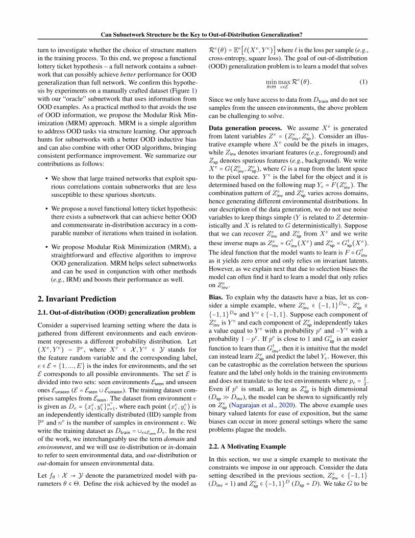
Figure 2. Left: OOD accuracy for four algorithms. Right: OODaccuracy for ERM algorithm and its digit module. The plot showsthat a highly biased model can contain an unbiased subnetwork.

sampling with parameters sigmoid(πl). We adopt Gumbel-sigmoid trick (Jang et al., 2016) to enable an end-to-endtraining process, together with a logit regularization termto promote subnetwork sparsity (Csordas et al., 2020). Foreach particular subtask, our analysis will output a logitstensor for each neuron in the form of π = {π1,⋯,πL},and thereby uncover the corresponding functional mod-ule within the neural network in the form of binary tensorm = {m1,⋯,mL} = {sigmoid(πl) > 0.5 ∣ l = 1,2,⋯}.We then use the term modularity probing method to refer tothis technique subsequently. We will interchangeably usethe term of module and subnetwork due to their consistencyin our context.

Dataset construction. We take the intuition from Arjovskyet al. (2019); Nam et al. (2020); Ahuja et al. (2021); Ahmedet al. (2021) to design a biased variant of the original MNISTdataset (LeCun et al., 1998). A discussion about the differ-ence between ours and theirs is deferred to supplementarymaterials. The digit shape semantics are considered as Zinv

while color semantics as Zsp. We choose ten different kindsof color and define a one-to-one corresponding bias rela-tionship with ten digit class (e.g., “2” ↔ “green”, “4” ↔“yellow” ). For each domain, we define the bias coefficientto be the ratio of the data that obeys this relationship. Thoseimages which don’t follow this relationship are then as-signed with random colors. The bias coefficient for twoin-domains is (1.0,0.9) respectively, which means the firstdomain is completely biased and 90 percent of the seconddomain is biased. For the out-domain, all images are as-signed a random color for evaluating to how much extentthe model has learned the invariant feature. The out-domainwill serve as a tool environment for module learning in thissection, representing a thorough disentanglement of twoattributions. It will then act as the test distribution in a re-alistic setting in Section 5. Unless otherwise specified, thelabel is set as the class where the invariant attribution lies.We use the term FULLCOLOREDMNIST to refer to thistask to distinguish with the binary colored mnist dataset inArjovsky et al. (2019).

Algorithms analyzed. We study four OOD generaliza-tion algorithms in this paper: Empirical Risk Minimization(ERM) (Vapnik, 1999), Invariant Risk Minimization (IRM)(Arjovsky et al., 2019), Risk Extrapolation (REx) (Kruegeret al., 2020) and group Distributional Robust Optimization(DRO) (Sagawa et al., 2019). More details about them areleft to supplementary materials. Figure 2(a) plots the gener-alization performance of these algorithms w.r.t. the trainingprocess. REx (76.17%) and DRO (78.56%) methods sur-pass ERM baseline by a large margin, while IRM (59.55%)only gets slightly better results than ERM (58.04 %). Thefailure of IRM in realistic problems has been analyzed inJin et al. (2020); Nagarajan et al. (2020); Rosenfeld et al.(2020); Ahuja et al. (2021) and attributed to the overparam-eterization regime and curse of dimensionality, hence weomit related discussion here.

3.2. Modular subnetwork introspection

Departing from previous approaches, in this section wethink of learning the digit and color semantics as differentfunctional subtasks of the original task, rather than oppositenon-spurious / spurious features. We split the out-domaininto two parts and refer to them as the in-split and out-splitof the out-domain (terminology from Gulrajani & Lopez-Paz (2020)). We define two subtasks, identification of digitand identification of color. For each subtask, we assume thatwe have access to respective semantic labels. It’s importantto note that the semantic color label is used here for analysisand is not a part of our main method described later.

In order to study the functional module for the two subtasks,we apply the modularity probing method to diagnose givenpretrained models. Specifically, we separately train and get adigit and a color subnetwork for each model across differentalgorithms and training steps. We evaluate the obtained digitmodules’ behaviors on the out-split of out-domain (as thein-split has been taken for module searching). Figure 2(b)suggests a significant evidence that, even for biased modelssuch as ERM trained ones, there exist unbiased invariantsubnetworks (digit modules) with good OOD generalizationability. We also explore this property for other modulesand algorithms and defer these results to supplementarymaterials.

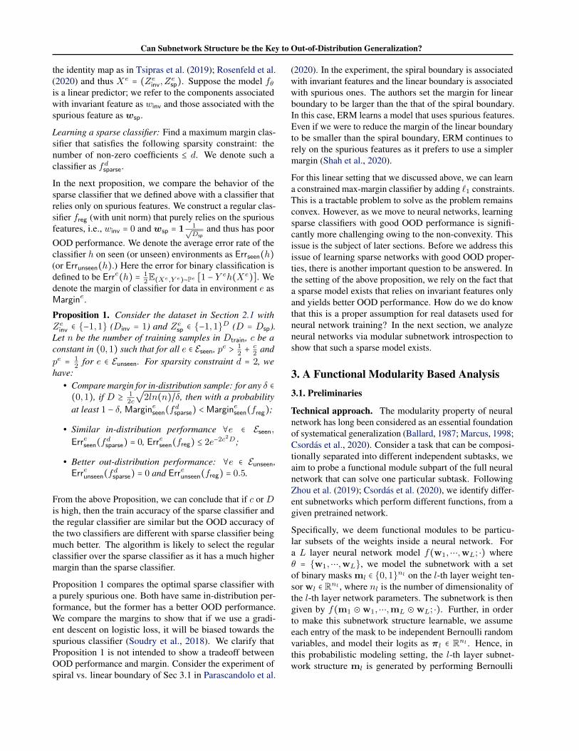
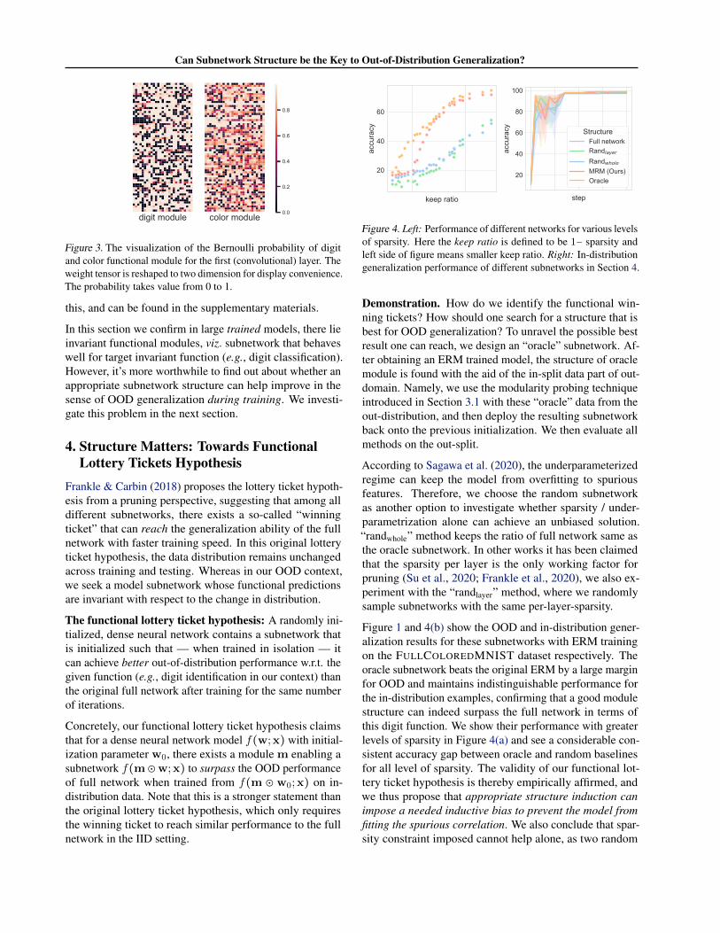
Discussion about the sparsity of digit weights / fea-tures. We additionally visualize the Bernoulli probabilityof learned subtask modules. Figure 3 displays the first layerof model trained on two in-domains with ERM. We cansee that the color feature is more pervasive than digit fea-ture, spreading over a broader range across the neurons.Although the sparsity of weights is not exactly the sparsityof features, the discovery is aligned with the assumption inProposition 1 that Dinv has a small number of dimensional-ity. The visualization results of other layers are similar to


digit module color module0.0

0.2

0.4

0.6

0.8

Figure 3. The visualization of the Bernoulli probability of digitand color functional module for the first (convolutional) layer. Theweight tensor is reshaped to two dimension for display convenience.The probability takes value from 0 to 1.

this, and can be found in the supplementary materials.

In this section we confirm in large trained models, there lieinvariant functional modules, viz. subnetwork that behaveswell for target invariant function (e.g., digit classification).However, it’s more worthwhile to find out about whether anappropriate subnetwork structure can help improve in thesense of OOD generalization during training. We investi-gate this problem in the next section.

4. Structure Matters: Towards FunctionalLottery Tickets Hypothesis

Frankle & Carbin (2018) proposes the lottery ticket hypoth-esis from a pruning perspective, suggesting that among alldifferent subnetworks, there exists a so-called “winningticket” that can reach the generalization ability of the fullnetwork with faster training speed. In this original lotteryticket hypothesis, the data distribution remains unchangedacross training and testing. Whereas in our OOD context,we seek a model subnetwork whose functional predictionsare invariant with respect to the change in distribution.

The functional lottery ticket hypothesis: A randomly ini-tialized, dense neural network contains a subnetwork thatis initialized such that — when trained in isolation — itcan achieve better out-of-distribution performance w.r.t. thegiven function (e.g., digit identification in our context) thanthe original full network after training for the same numberof iterations.

Concretely, our functional lottery ticket hypothesis claimsthat for a dense neural network model f(w;x) with initial-ization parameter w0, there exists a module m enabling asubnetwork f(m⊙w;x) to surpass the OOD performanceof full network when trained from f(m ⊙ w0;x) on in-distribution data. Note that this is a stronger statement thanthe original lottery ticket hypothesis, which only requiresthe winning ticket to reach similar performance to the fullnetwork in the IID setting.

keep ratio

20

40

60

accu

racy

step

20

40

60

80

100

accu

racy Structure

Full networkRandlayer

Randwhole

MRM (Ours)Oracle

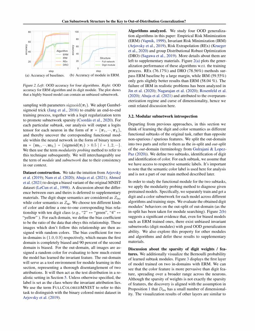
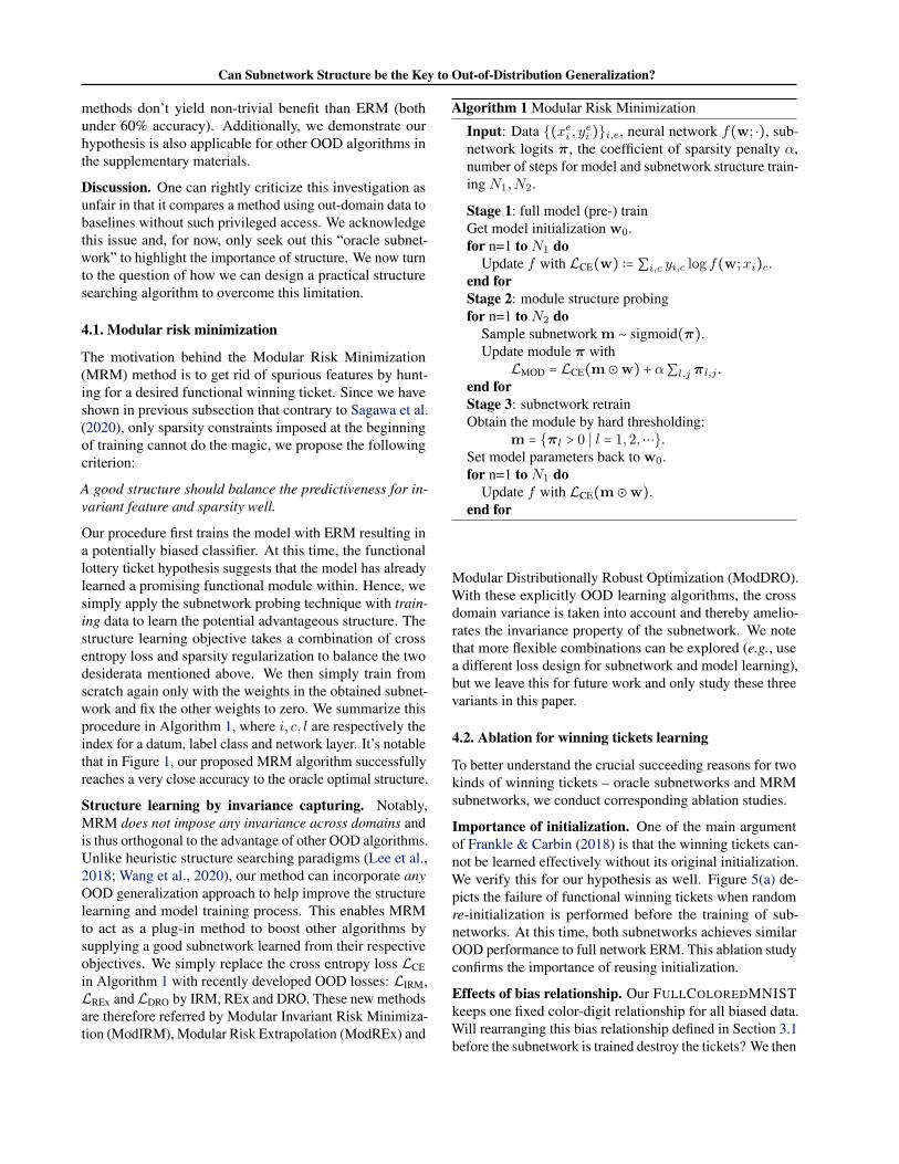
Figure 4. Left: Performance of different networks for various levelsof sparsity. Here the keep ratio is defined to be 1− sparsity andleft side of figure means smaller keep ratio. Right: In-distributiongeneralization performance of different subnetworks in Section 4.

Demonstration. How do we identify the functional win-ning tickets? How should one search for a structure that isbest for OOD generalization? To unravel the possible bestresult one can reach, we design an “oracle” subnetwork. Af-ter obtaining an ERM trained model, the structure of oraclemodule is found with the aid of the in-split data part of out-domain. Namely, we use the modularity probing techniqueintroduced in Section 3.1 with these “oracle” data from theout-distribution, and then deploy the resulting subnetworkback onto the previous initialization. We then evaluate allmethods on the out-split.

According to Sagawa et al. (2020), the underparameterizedregime can keep the model from overfitting to spuriousfeatures. Therefore, we choose the random subnetworkas another option to investigate whether sparsity / under-parametrization alone can achieve an unbiased solution.“randwhole” method keeps the ratio of full network same asthe oracle subnetwork. In other works it has been claimedthat the sparsity per layer is the only working factor forpruning (Su et al., 2020; Frankle et al., 2020), we also ex-periment with the “randlayer” method, where we randomlysample subnetworks with the same per-layer-sparsity.

Figure 1 and 4(b) show the OOD and in-distribution gener-alization results for these subnetworks with ERM trainingon the FULLCOLOREDMNIST dataset respectively. Theoracle subnetwork beats the original ERM by a large marginfor OOD and maintains indistinguishable performance forthe in-distribution examples, confirming that a good modulestructure can indeed surpass the full network in terms ofthis digit function. We show their performance with greaterlevels of sparsity in Figure 4(a) and see a considerable con-sistent accuracy gap between oracle and random baselinesfor all level of sparsity. The validity of our functional lot-tery ticket hypothesis is thereby empirically affirmed, andwe thus propose that appropriate structure induction canimpose a needed inductive bias to prevent the model fromfitting the spurious correlation. We also conclude that spar-sity constraint imposed cannot help alone, as two random


methods don’t yield non-trivial benefit than ERM (bothunder 60% accuracy). Additionally, we demonstrate ourhypothesis is also applicable for other OOD algorithms inthe supplementary materials.

Discussion. One can rightly criticize this investigation asunfair in that it compares a method using out-domain data tobaselines without such privileged access. We acknowledgethis issue and, for now, only seek out this “oracle subnet-work” to highlight the importance of structure. We now turnto the question of how we can design a practical structuresearching algorithm to overcome this limitation.

4.1. Modular risk minimization

The motivation behind the Modular Risk Minimization(MRM) method is to get rid of spurious features by hunt-ing for a desired functional winning ticket. Since we haveshown in previous subsection that contrary to Sagawa et al.(2020), only sparsity constraints imposed at the beginningof training cannot do the magic, we propose the followingcriterion:

A good structure should balance the predictiveness for in-variant feature and sparsity well.

Our procedure first trains the model with ERM resulting ina potentially biased classifier. At this time, the functionallottery ticket hypothesis suggests that the model has alreadylearned a promising functional module within. Hence, wesimply apply the subnetwork probing technique with train-ing data to learn the potential advantageous structure. Thestructure learning objective takes a combination of crossentropy loss and sparsity regularization to balance the twodesiderata mentioned above. We then simply train fromscratch again only with the weights in the obtained subnet-work and fix the other weights to zero. We summarize thisprocedure in Algorithm 1, where i, c, l are respectively theindex for a datum, label class and network layer. It’s notablethat in Figure 1, our proposed MRM algorithm successfullyreaches a very close accuracy to the oracle optimal structure.

Structure learning by invariance capturing. Notably,MRM does not impose any invariance across domains andis thus orthogonal to the advantage of other OOD algorithms.Unlike heuristic structure searching paradigms (Lee et al.,2018; Wang et al., 2020), our method can incorporate anyOOD generalization approach to help improve the structurelearning and model training process. This enables MRMto act as a plug-in method to boost other algorithms bysupplying a good subnetwork learned from their respectiveobjectives. We simply replace the cross entropy loss LCEin Algorithm 1 with recently developed OOD losses: LIRM,LREx and LDRO by IRM, REx and DRO. These new methodsare therefore referred by Modular Invariant Risk Minimiza-tion (ModIRM), Modular Risk Extrapolation (ModREx) and

Algorithm 1 Modular Risk Minimization

Input: Data {(xei , yei )}i,e, neural network f(w; ⋅), sub-network logits π, the coefficient of sparsity penalty α,number of steps for model and subnetwork structure train-ing N1,N2.

Stage 1: full model (pre-) trainGet model initialization w0.for n=1 to N1 do

Update f with LCE(w) ∶= ∑i,c yi,c log f(w;xi)c.end forStage 2: module structure probingfor n=1 to N2 do

Sample subnetwork m ∼ sigmoid(π).Update module π with

LMOD = LCE(m⊙w) + α∑l,j πl,j .end forStage 3: subnetwork retrainObtain the module by hard thresholding:

m = {πl > 0 ∣ l = 1,2,⋯}.Set model parameters back to w0.for n=1 to N1 do

Update f with LCE(m⊙w).end for

Modular Distributionally Robust Optimization (ModDRO).With these explicitly OOD learning algorithms, the crossdomain variance is taken into account and thereby amelio-rates the invariance property of the subnetwork. We notethat more flexible combinations can be explored (e.g., usea different loss design for subnetwork and model learning),but we leave this for future work and only study these threevariants in this paper.

4.2. Ablation for winning tickets learning

To better understand the crucial succeeding reasons for twokinds of winning tickets – oracle subnetworks and MRMsubnetworks, we conduct corresponding ablation studies.

Importance of initialization. One of the main argumentof Frankle & Carbin (2018) is that the winning tickets can-not be learned effectively without its original initialization.We verify this for our hypothesis as well. Figure 5(a) de-picts the failure of functional winning tickets when randomre-initialization is performed before the training of sub-networks. At this time, both subnetworks achieves similarOOD performance to full network ERM. This ablation studyconfirms the importance of reusing initialization.

Effects of bias relationship. Our FULLCOLOREDMNISTkeeps one fixed color-digit relationship for all biased data.Will rearranging this bias relationship defined in Section 3.1before the subnetwork is trained destroy the tickets? We then


step

10

20

30

40

50

60

70

accu

racy

StructureFull networkreinit-MRMreinit-OracleMRMOracle

step

10

20

30

40

50

60

70

accu

racy

StructureFull networkrebias-MRMrebias-OracleMRMOracle

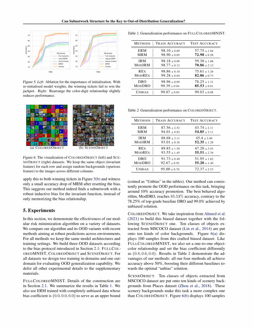
Figure 5. Left: Ablation for the importance of initialization. Withre-initialized model weights, the winning tickets fail to win thejackpot. Right: Rearrange the color-digit relationship slightlyreduces performance.

(a) COLOREDOBJECT (b) SCENEOBJECT

Figure 6. The visualization of COLOREDOBJECT (left) and SCE-NEOBJECT (right) datasets. We keep the same object (invariantfeature) for each row and assign random backgrounds (spuriousfeature) to the images across different columns.

apply this to both winning tickets in Figure 5(b) and witnessonly a small accuracy drop of MRM after resetting the bias.This suggests our method indeed finds a subnetwork with arobust inductive bias for the invariant function, instead ofonly memorizing the bias relationship.

5. ExperimentsIn this section, we demonstrate the effectiveness of our mod-ular risk minimization algorithm on a variety of datasets.We compare our algorithm and its OOD variants with recentmethods aiming at robust predictions across environments.For all methods we keep the same model architectures andtraining settings. We build three OOD datasets accordingto the bias protocol introduced in Section 2.1: FULLCOL-OREDMNIST, COLOREDOBJECT and SCENEOBJECT. Forall datasets we design two training in-domains and one out-domain for evaluating OOD generalization capability. Wedefer all other experimental details to the supplementarymaterials.

FULLCOLOREDMNIST. Details of the construction arein Section 2.1. We summarize the results in Table 1. Wealso use ERM trained with completely unbiased data whosebias coefficient is (0.0,0.0,0.0) to serve as an upper bound

Table 1. Generalization performance on FULLCOLOREDMNIST.

METHODS TRAIN ACCURACY TEST ACCURACY

ERM 98.10 ± 0.09 57.75 ± 1.84MRM 98.90 ± 0.05 72.98 ± 0.58

IRM 98.18 ± 0.09 59.30 ± 1.88MODIRM 98.77 ± 0.12 70.86 ± 2.12

REX 98.86 ± 0.10 75.61 ± 1.26MODREX 99.28 ± 0.04 82.06 ± 0.73

DRO 98.96 ± 0.09 78.25 ± 1.31MODDRO 99.39 ± 0.04 85.53 ± 0.61

UNBIAS 99.07 ± 0.04 99.03 ± 0.08

Table 2. Generalization performance on COLOREDOBJECT.


ERM 87.56 ± 2.52 43.74 ± 2.11MRM 94.01 ± 0.82 54.85 ± 2.11

IRM 88.68 ± 2.11 45.4 ± 2.40MODIRM 93.01 ± 0.36 52.35 ± 1.28

REX 89.85 ± 1.50 47.20 ± 3.43MODREX 93.55 ± 1.45 55.51 ± 2.76

DRO 91.73 ± 0.40 51.95 ± 1.62MODDRO 92.67 ± 0.92 55.20 ± 1.40

UNBIAS 95.00 ± 0.70 72.37 ± 2.53

(coined as “Unbias” in the tables). Our method can consis-tently promote the OOD performance on this task, bringingaround 10% accuracy promotion. The best behaved algo-rithm, ModDRO, reaches 85.53% accuracy, contrary to the78.25% of top-grade baseline DRO and 99.0% achieved byunbiased solution.

COLOREDOBJECT. We take inspiration from Ahmed et al.(2021) to build this biased dataset together with the fol-lowing SCENEOBJECT one. Ten classes of objects ex-tracted from MSCOCO dataset (Lin et al., 2014) are putonto ten kinds of color backgrounds. Figure 6(a) dis-plays 100 samples from this crafted biased dataset. LikeFULLCOLOREDMNIST, we also set a one-to-one object-color relationship and set the bias coefficient differentlyas (0.8,0.6,0.0). Results in Table 2 demonstrate the ad-vantages of our methods: all our four methods all achieveaccuracy above 50%, boosting their different baselines to-wards the optimal “unbias” solution.

SCENEOBJECT. Ten classes of objects extracted fromMSCOCO dataset are put onto ten kinds of scenery back-grounds from Places dataset (Zhou et al., 2018). Thesescenery backgrounds make this task a more complex onethan COLOREDOBJECT. Figure 6(b) displays 100 samples


Table 3. Generalization performance on SCENEOBJECT.


ERM 98.87 ± 0.23 37.29 ± 2.74MRM 99.61 ± 0.04 39.44 ± 0.77

IRM 98.68 ± 0.27 37.19 ± 2.58MODIRM 99.39 ± 0.01 39.14 ± 1.34

REX 92.91 ± 1.11 38.84 ± 1.39MODREX 96.71 ± 0.53 41.04 ± 1.46

DRO 98.89 ± 0.35 36.34 ± 1.67MODDRO 99.41 ± 0.13 39.14 ± 1.60

UNBIAS 95.25 ± 2.21 56.46 ± 0.75

from this crafted dataset. Like FULLCOLOREDMNIST, weset a one-to-one object-scenery relationship and set the biascoefficient to be (0.9,0.7,0.0), making it a even more bi-ased and thus more difficult one than the previous task. Thiscan also be shown with only 56.46% accuracy of unbias so-lution. Corresponding results in Table 3 shows that for thishighly biased task, MRM and its variants can still accord-ingly improve out-distribution generalization performancein this highly bias setting, where previous OOD algorithmsbring very limited benefit.

6. Related WorkOut-of-distribution generalization. Machine learning be-yond IID assumption is a very important problem and manyresearch areas such as domain adaptation (Crammer et al.,2008; Ben-David et al., 2010) and domain generalization(Muandet et al., 2013; Motiian et al., 2017) have receivedmuch attention (Gulrajani & Lopez-Paz, 2020). To get sta-ble prediction for new unseen data distribution, it is desiredto only rely on invariant features among the causal factoriza-tion of physical mechanisms of problem settings (Scholkopfet al., 2012). Peters et al. (2016) (ICP) claims that theresidual of invariant method should remain IID and thus pro-poses to adopt statistical tests for mining invariant featureset. Rojas-Carulla et al. (2018) generalizes this approach tononlinear settings.

Recently, since Arjovsky et al. (2019) brings invariant pre-diction into a more practical scenario, a large amount ofworks has made solid progress for alleviating spurious cor-relation and shortcut exploitation (Geirhos et al., 2020; Kohet al., 2020): Sagawa et al. (2019) proposes to use groupDRO when attribution information is provided; Chang et al.(2020) incorporates this invariant inference idea into se-lective rationalization area; Ahuja et al. (2020) studies theIRM formulation from a game theory and bilevel optimiza-tion formulation; Krueger et al. (2020) propose REx toenforce the variance of losses across distribution, which isfurther analyzed by Xie et al. (2020a); Koyama & Yam-aguchi (2020) (IGA) also has a similar contribution with dif-

ferent theoretical analysis; Jin et al. (2020) (RGM) proposesanother training objective from regret minimization view-point; Pezeshki et al. (2020) studies the gradient starvationphenomenon which is connected with spurious correlationand proposes an insightful solution; Creager et al. (2020)(EIIL) points out that invariant prediction shares the samespirit with fair representation learning; Parascandolo et al.(2020) (ILC) proposes to focus second order landscape in-formation; Ahmed et al. (2021) adopts a divergence term tomatch the output distribution spaces of different domains;Muller et al. (2020) achieves invariance from an informationtheory start point and enforces conditional invariance withHSIC terms. Some other works also point out the pitfalls ofcurrent approaches, showing only in very limited situationscan Arjovsky et al. (2019) (e.g., low dimension settings)really capture invariance: Rosenfeld et al. (2020) proves thevalidity of IRM for linear cases but gives a negative exam-ple for nonlinear cases; Nagarajan et al. (2020) analyzesdifferent failure modes of OOD generalization; Ahuja et al.(2021) analyze the sample efficiency properties of IRM;Kamath et al. (2021) investigates the success and failurecases of IRM and IRMv1 on simple but insightful settings,and claims the community might need a better invariancenotion.

Another line of works study a related but different topicnamed debiasing, where there is no explicit multiple en-vironments setting provided. Bias in realistic datasets areusually exploited in a spurious way, such as the texture-biasof Imagenet-trained models (Geirhos et al., 2018). Subse-quent works (Wang et al., 2019; Bahng et al., 2020; Shiet al., 2020; Nam et al., 2020; Li et al., 2021; Sauer &Geiger, 2021) focus on addressing the bias problem withexplicit debiasing procedure.

Modularity. Modularity (Ballard, 1987; Fodor et al., 1988;Newman, 2006) has been considered as a crucial part of in-telligent systems. Lots of works focus on imposing explicitmodule level modularity (Clune et al., 2013; Andreas et al.,2016; Chang et al., 2018; Goyal et al., 2021), while othersalso explore weight level modularity in a more fine-grainedway (Mallya & Lazebnik, 2018; Watanabe et al., 2019; Filanet al., 2020; Csordas et al., 2020). Our work also belongs tothe latter category.

Pruning. We mainly focus on unstructured pruning litera-ture. This line of model compression literature dates back toMozer & Smolensky (1989); LeCun et al. (1989); Hassibi& Stork (1993) with more recent pruning methods (Hanet al., 2015; Molchanov et al., 2016; Dong et al., 2017).Recently, the lottery ticket hypothesis (Frankle & Carbin,2018) sheds more light into this field, showing the impor-tance of initialization. (Liu et al., 2018) also propose anotherviewpoint that for practical settings the inherited weightsare not important.


7. DiscussionData settings. The seminal work (Arjovsky et al., 2019)proposes to use color in digit identification as a spuriouscorrelation. In order to exposit the effectiveness of IRM,the authors enforce a 25% label noise in the binary classi-fication data and assign color a larger correlation than thetrue digit shape. In this way, ERM exploits color feature topredict. While there is controversy surrounding whether oneshould still treat digit as desired learning target under thissituation, we choose to impose no label noise in FULLCOL-OREDMNIST as is the case in Nam et al. (2020); Ahmedet al. (2021). This choice enables the structure learning pro-cedure could mine the true invariant feature. On the otherhand, our work is limited as we haven’t considered the datasettings such as group attribution available ones (Sagawaet al., 2019; Xie et al., 2020b; Khani & Liang, 2021) andwe shall fill this gap in future work. More about datasetscan be found in Section C.1.

Success of MRM. There are several reasons for why MRMcan improve OOD performance without invariance con-strain. The first reason is related to our label noise freesetting discussed above. This makes the invariant featureitself perfectly predictive of the label, thus containing allinformation about the desired target function. Then the prob-lem would be how to exploit this information effectively.MRM becomes competent for OOD tasks by providing anovel and helpful parameterization method for the originaloptimization problem with extra parameters. One notablething is that more structure parameters actually don’t in-crease the expressive power of the neural network, sinceevery weight can take zero value in nature. Another reasonis we adopt an explicit approach to zero out the “spuriouspart” of the model weights, hence achieving a not-so-biasedsolution. Notice this cannot be achieved with random sparsemodel, revealing the structure is a key element for OODgeneralization. Therefore, a positive answer is given to thetitle of this work. We further refer to Section C.3 for empir-ical results of the importance of a proper sparsity level instructure learning.

AcknowledgementKartik Ahuja acknowledges the support provided by IVADOpostdoctoral fellowship funding program. Yilun Xu issupported by the MIT HDTV Grand Alliance Fellowship.Yisen Wang is partially supported by the National NaturalScience Foundation of China under Grant 62006153, andCCF-Baidu Open Fund (OF2020002). Aaron Courvilleacknowledges the funding from CIFAR Canadian AIChair and Hitachi. The authors would also like to thankRobert Csordas, David Krueger, Faruk Ahmed, Moham-mad Pezeshki, Baifeng Shi, Sara Hooker and anonymousreviewers for insightful discussion and feedbacks.

ReferencesAhmed, F., Bengio, Y., van Seijen, H., and Courville, A. Sys-

tematic generalisation with group invariant predictions.In International Conference on Learning Representations,2021. URL https://openreview.net/forum?id=b9PoimzZFJ.

Ahuja, K., Shanmugam, K., Varshney, K., and Dhurandhar,A. Invariant risk minimization games. In InternationalConference on Machine Learning, pp. 145–155. PMLR,2020.

Ahuja, K., Wang, J., Dhurandhar, A., Shanmugam, K., andVarshney, K. R. Empirical or invariant risk minimization?a sample complexity perspective. In International Confer-ence on Learning Representations, 2021. URL https://openreview.net/forum?id=jrA5GAccy_.

Andreas, J., Rohrbach, M., Darrell, T., and Klein, D. Neuralmodule networks. In Proceedings of the IEEE conferenceon computer vision and pattern recognition, pp. 39–48,2016.

Arjovsky, M., Bottou, L., Gulrajani, I., and Lopez-Paz,D. Invariant risk minimization. ArXiv, abs/1907.02893,2019.

Bahng, H., Chun, S., Yun, S., Choo, J., and Oh, S. J. Learn-ing de-biased representations with biased representations.In International Conference on Machine Learning, pp.528–539. PMLR, 2020.

Ballard, D. H. Modular learning in neural networks. InAAAI, pp. 279–284, 1987.

Beery, S., Van Horn, G., and Perona, P. Recognition in terraincognita. In Proceedings of the European Conferenceon Computer Vision, pp. 456–473, 2018.

Ben-David, S., Blitzer, J., Crammer, K., Kulesza, A.,Pereira, F., and Vaughan, J. W. A theory of learningfrom different domains. Machine learning, 79(1):151–175, 2010.

Bengio, Y., Deleu, T., Rahaman, N., Ke, R., Lachapelle,S., Bilaniuk, O., Goyal, A., and Pal, C. A meta-transferobjective for learning to disentangle causal mechanisms.arXiv preprint arXiv:1901.10912, 2019.

Brendel, W. and Bethge, M. Approximating cnns withbag-of-local-features models works surprisingly well onimagenet. arXiv preprint arXiv:1904.00760, 2019.

Chang, M. B., Gupta, A., Levine, S., and Griffiths,T. L. Automatically composing representation transfor-mations as a means for generalization. arXiv preprintarXiv:1807.04640, 2018.

https://openreview.net/forum?id=b9PoimzZFJ

https://openreview.net/forum?id=b9PoimzZFJ

https://openreview.net/forum?id=jrA5GAccy_

https://openreview.net/forum?id=jrA5GAccy_


Chang, S., Zhang, Y., Yu, M., and Jaakkola, T. Invariantrationalization. In International Conference on MachineLearning, pp. 1448–1458. PMLR, 2020.

Clune, J., Mouret, J.-B., and Lipson, H. The evolutionaryorigins of modularity. Proceedings of the Royal Societyb: Biological sciences, 280(1755):20122863, 2013.

Crammer, K., Kearns, M., and Wortman, J. Learning frommultiple sources. Journal of Machine Learning Research,9(8), 2008.

Creager, E., Jacobsen, J.-H., and Zemel, R. Exchanginglessons between algorithmic fairness and domain gener-alization. arXiv preprint arXiv:2010.07249, 2020.

Csordas, R., van Steenkiste, S., and Schmidhuber, J. Areneural nets modular? inspecting functional modular-ity through differentiable weight masks. arXiv preprintarXiv:2010.02066, 2020.

DeGrave, A. J., Janizek, J. D., and Lee, S.-I. Ai for radio-graphic covid-19 detection selects shortcuts over signal.medRxiv, 2020.

Dong, X., Chen, S., and Pan, S. J. Learning to prune deepneural networks via layer-wise optimal brain surgeon.arXiv preprint arXiv:1705.07565, 2017.

Filan, D., Hod, S., Wild, C., Critch, A., and Russell, S.Neural networks are surprisingly modular. arXiv preprintarXiv:2003.04881, 2020.

Fodor, J. A., Pylyshyn, Z. W., et al. Connectionism andcognitive architecture: A critical analysis. Cognition, 28(1-2):3–71, 1988.

Frankle, J. and Carbin, M. The lottery ticket hypothesis:Finding sparse, trainable neural networks. arXiv preprintarXiv:1803.03635, 2018.

Frankle, J., Dziugaite, G. K., Roy, D. M., and Carbin, M.Pruning neural networks at initialization: Why are wemissing the mark? arXiv preprint arXiv:2009.08576,2020.

Geirhos, R., Rubisch, P., Michaelis, C., Bethge, M., Wich-mann, F. A., and Brendel, W. Imagenet-trained cnns arebiased towards texture; increasing shape bias improves ac-curacy and robustness. arXiv preprint arXiv:1811.12231,2018.

Geirhos, R., Jacobsen, J.-H., Michaelis, C., Zemel, R., Bren-del, W., Bethge, M., and Wichmann, F. A. Shortcut learn-ing in deep neural networks. Nature Machine Intelligence,2(11):665–673, 2020.

Goyal, A., Lamb, A., Hoffmann, J., Sodhani, S., Levine,S., Bengio, Y., and Scholkopf, B. Recurrent independentmechanisms. In International Conference on LearningRepresentations, 2021. URL https://openreview.net/forum?id=mLcmdlEUxy-.

Gulrajani, I. and Lopez-Paz, D. In search of lost domaingeneralization. arXiv preprint arXiv:2007.01434, 2020.

Han, S., Mao, H., and Dally, W. J. Deep compres-sion: Compressing deep neural networks with pruning,trained quantization and huffman coding. arXiv preprintarXiv:1510.00149, 2015.

Hassibi, B. and Stork, D. G. Second order derivativesfor network pruning: Optimal brain surgeon. MorganKaufmann, 1993.

Hooker, S., Courville, A., Clark, G., Dauphin, Y., andFrome, A. What do compressed deep neural networksforget? arXiv preprint arXiv:1911.05248, 2019.

Hooker, S., Moorosi, N., Clark, G., Bengio, S., and Denton,E. Characterising bias in compressed models. arXivpreprint arXiv:2010.03058, 2020.

Jang, E., Gu, S., and Poole, B. Categorical repa-rameterization with gumbel-softmax. arXiv preprintarXiv:1611.01144, 2016.

Jin, W., Barzilay, R., and Jaakkola, T. Domain ex-trapolation via regret minimization. arXiv preprintarXiv:2006.03908, 2020.

Kamath, P., Tangella, A., Sutherland, D. J., and Srebro,N. Does invariant risk minimization capture invariance?arXiv preprint arXiv:2101.01134, 2021.

Khani, F. and Liang, P. Removing spurious features canhurt accuracy and affect groups disproportionately. InACM Conference on Fairness, Accountability, and Trans-parency (FAccT), 2021.

Koh, P. W., Sagawa, S., Marklund, H., Xie, S. M., Zhang,M., Balsubramani, A., Hu, W., Yasunaga, M., Phillips,R. L., Beery, S., et al. Wilds: A benchmark of in-the-wild distribution shifts. arXiv preprint arXiv:2012.07421,2020.

Koyama, M. and Yamaguchi, S. Out-of-distribution general-ization with maximal invariant predictor. arXiv preprintarXiv:2008.01883, 2020.

Krueger, D., Caballero, E., Jacobsen, J., Zhang, A., Bi-nas, J., Priol, R. L., and Courville, A. C. Out-of-distribution generalization via risk extrapolation (rex).ArXiv, abs/2003.00688, 2020.

https://openreview.net/forum?id=mLcmdlEUxy-

https://openreview.net/forum?id=mLcmdlEUxy-


LeCun, Y., Denker, J. S., Solla, S. A., Howard, R. E., andJackel, L. D. Optimal brain damage. In NIPs, volume 2,pp. 598–605. Citeseer, 1989.

LeCun, Y., Bottou, L., Bengio, Y., and Haffner, P. Gradient-based learning applied to document recognition. Proceed-ings of the IEEE, 86(11):2278–2324, 1998.

Lee, N., Ajanthan, T., and Torr, P. H. Snip: Single-shotnetwork pruning based on connection sensitivity. arXivpreprint arXiv:1810.02340, 2018.

Li, Y., Yu, Q., Tan, M., Mei, J., Tang, P., Shen, W., Yuille,A., and cihang xie. Shape-texture debiased neural net-work training. In International Conference on LearningRepresentations, 2021. URL https://openreview.net/forum?id=Db4yerZTYkz.

Lin, T. Y., Maire, M., Belongie, S., Hays, J., and Zitnick,C. L. Microsoft coco: Common objects in context. InEuropean Conference on Computer Vision, 2014.

Liu, Z., Sun, M., Zhou, T., Huang, G., and Darrell, T. Re-thinking the value of network pruning. arXiv preprintarXiv:1810.05270, 2018.

Louizos, C., Welling, M., and Kingma, D. P. Learningsparse neural networks through l0 regularization. ArXiv,abs/1712.01312, 2018.

Mallya, A. and Lazebnik, S. Packnet: Adding multiple tasksto a single network by iterative pruning. In Proceedingsof the IEEE Conference on Computer Vision and PatternRecognition, pp. 7765–7773, 2018.

Marcus, G. F. Rethinking eliminative connectionism. Cog-nitive psychology, 37(3):243–282, 1998.

Mocanu, D. C., Mocanu, E., Stone, P., Nguyen, P. H.,Gibescu, M., and Liotta, A. Scalable training of arti-ficial neural networks with adaptive sparse connectivityinspired by network science. Nature communications, 9(1):1–12, 2018.

Molchanov, P., Tyree, S., Karras, T., Aila, T., and Kautz,J. Pruning convolutional neural networks for resourceefficient inference. arXiv preprint arXiv:1611.06440,2016.

Mostafa, H. and Wang, X. Parameter efficient training ofdeep convolutional neural networks by dynamic sparsereparameterization. In International Conference on Ma-chine Learning, pp. 4646–4655. PMLR, 2019.

Motiian, S., Piccirilli, M., Adjeroh, D. A., and Doretto,G. Unified deep supervised domain adaptation and gen-eralization. In Proceedings of the IEEE internationalconference on computer vision, pp. 5715–5725, 2017.

Mozer, M. C. and Smolensky, P. Skeletonization: A Tech-nique for Trimming the Fat from a Network via RelevanceAssessment. Morgan Kaufmann Publishers Inc., 1989.

Muandet, K., Balduzzi, D., and Scholkopf, B. Domaingeneralization via invariant feature representation. InInternational Conference on Machine Learning, pp. 10–18. PMLR, 2013.

Muller, J., Schmier, R., Ardizzone, L., Rother, C., andKothe, U. Learning robust models using the princi-ple of independent causal mechanisms. arXiv preprintarXiv:2010.07167, 2020.

Nagarajan, V., Andreassen, A., and Neyshabur, B. Under-standing the failure modes of out-of-distribution general-ization. arXiv preprint arXiv:2010.15775, 2020.

Nam, J., Cha, H., Ahn, S., Lee, J., and Shin, J. Learningfrom failure: Training debiased classifier from biasedclassifier. arXiv preprint arXiv:2007.02561, 2020.

Newman, M. E. Modularity and community structure in net-works. Proceedings of the national academy of sciences,103(23):8577–8582, 2006.

Parascandolo, G., Neitz, A., Orvieto, A., Gresele, L., andScholkopf, B. Learning explanations that are hard to vary.arXiv preprint arXiv:2009.00329, 2020.

Peters, J., Buhlmann, P., and Meinshausen, N. Causal in-ference by using invariant prediction: identification andconfidence intervals. Journal of the Royal Statistical So-ciety. Series B (Statistical Methodology), pp. 947–1012,2016.

Pezeshki, M., Kaba, S.-O., Bengio, Y., Courville, A., Precup,D., and Lajoie, G. Gradient starvation: A learning procliv-ity in neural networks. arXiv preprint arXiv:2011.09468,2020.

Priol, R. L., Harikandeh, R. B., Bengio, Y., and Lacoste-Julien, S. An analysis of the adaptation speed of causalmodels. arXiv preprint arXiv:2005.09136, 2020.

Ritter, S., Barrett, D. G., Santoro, A., and Botvinick, M. M.Cognitive psychology for deep neural networks: A shapebias case study. In International conference on machinelearning, pp. 2940–2949. PMLR, 2017.

Rojas-Carulla, M., Scholkopf, B., Turner, R., and Peters, J.Invariant models for causal transfer learning. The Journalof Machine Learning Research, 19(1):1309–1342, 2018.

Rosenfeld, E., Ravikumar, P., and Risteski, A. Therisks of invariant risk minimization. arXiv preprintarXiv:2010.05761, 2020.

https://openreview.net/forum?id=Db4yerZTYkz

https://openreview.net/forum?id=Db4yerZTYkz


Sagawa, S., Koh, P. W., Hashimoto, T. B., and Liang, P.Distributionally robust neural networks for group shifts:On the importance of regularization for worst-case gener-alization. arXiv preprint arXiv:1911.08731, 2019.

Sagawa, S., Raghunathan, A., Koh, P. W., and Liang, P. Aninvestigation of why overparameterization exacerbatesspurious correlations. In International Conference onMachine Learning, pp. 8346–8356. PMLR, 2020.

Sauer, A. and Geiger, A. Counterfactual generative net-works. In International Conference on Learning Rep-resentations, 2021. URL https://openreview.net/forum?id=BXewfAYMmJw.

Scholkopf, B., Janzing, D., Peters, J., Sgouritsa, E., Zhang,K., and Mooij, J. On causal and anticausal learning. arXivpreprint arXiv:1206.6471, 2012.

Shah, H., Tamuly, K., Raghunathan, A., Jain, P., and Netra-palli, P. The pitfalls of simplicity bias in neural networks.arXiv preprint arXiv:2006.07710, 2020.

Shi, B., Zhang, D., Dai, Q., Zhu, Z., Mu, Y., and Wang, J.Informative dropout for robust representation learning: Ashape-bias perspective. In International Conference onMachine Learning, pp. 8828–8839. PMLR, 2020.

Soudry, D., Hoffer, E., Nacson, M. S., Gunasekar, S., andSrebro, N. The implicit bias of gradient descent on sepa-rable data. The Journal of Machine Learning Research,19(1):2822–2878, 2018.

Srivastava, N., Hinton, G., Krizhevsky, A., Sutskever, I.,and Salakhutdinov, R. Dropout: a simple way to preventneural networks from overfitting. The journal of machinelearning research, 15(1):1929–1958, 2014.

Su, J., Chen, Y., Cai, T., Wu, T., Gao, R., Wang, L., and Lee,J. D. Sanity-checking pruning methods: Random ticketscan win the jackpot. arXiv preprint arXiv:2009.11094,2020.

Tsipras, D., Santurkar, S., Engstrom, L., Turner, A., andMadry, A. Robustness may be at odds with accuracy,2019.

Vapnik, V. N. An overview of statistical learning theory.IEEE transactions on neural networks, 10(5):988–999,1999.

Wang, C., Zhang, G., and Grosse, R. Picking winningtickets before training by preserving gradient flow. arXivpreprint arXiv:2002.07376, 2020.

Wang, H., He, Z., Lipton, Z. C., and Xing, E. P. Learningrobust representations by projecting superficial statisticsout. arXiv preprint arXiv:1903.06256, 2019.

Watanabe, C., Hiramatsu, K., and Kashino, K. Understand-ing community structure in layered neural networks. Neu-rocomputing, 367:84–102, 2019.

Xie, C., Chen, F., Liu, Y., and Li, Z. Risk variance penaliza-tion: From distributional robustness to causality. arXivpreprint arXiv:2006.07544, 2020a.

Xie, S. M., Kumar, A., Jones, R., Khani, F., Ma, T., andLiang, P. In-n-out: Pre-training and self-training usingauxiliary information for out-of-distribution robustness.arXiv preprint arXiv:2012.04550, 2020b.

Zagoruyko, S. and Komodakis, N. Wide residual networks.arXiv preprint arXiv:1605.07146, 2016.

Zeiler, M. D. and Fergus, R. Visualizing and understand-ing convolutional networks. In European conference oncomputer vision, pp. 818–833. Springer, 2014.

Zeng, W. and Urtasun, R. Mlprune: Multi-layer pruning forautomated neural network compression. 2018.

Zhou, B., Lapedriza, A., Khosla, A., Oliva, A., and Torralba,A. Places: A 10 million image database for scene recog-nition. IEEE Trans Pattern Anal Mach Intell, pp. 1–1,2018.

Zhou, H., Lan, J., Liu, R., and Yosinski, J. Deconstruct-ing lottery tickets: Zeros, signs, and the supermask. InAdvances in Neural Information Processing Systems, pp.3597–3607, 2019.

Zhu, M. and Gupta, S. To prune, or not to prune: exploringthe efficacy of pruning for model compression. arXivpreprint arXiv:1710.01878, 2017.

https://openreview.net/forum?id=BXewfAYMmJw

https://openreview.net/forum?id=BXewfAYMmJw


A. Omitted ProofA.1. Proof for Proposition 1

Proof. We first analyze the performance of freg. The prediction from this classifier is Y e = sgn(wTspuZ

esp), thus

wTspuZ

esp =

1√D

D

∑i=1

Zesp,i =√D[ 1

D

D

∑i=1

Zesp,i],

Y e = sgn(wTspuZ

esp) = sgn[ 1

D

D

∑i=1

Zesp,i].(2)

We then analyze the error for any environment:

Erre = 1

2[1 −Ee[Y eY e]],

Ee[Y eY e] = Ee[sgn[ 1

D

D

∑i=1

Zesp,i]Y e] = ∑y∈{−1,1}

P[Y e = y]Ee[sgn( 1

D

D

∑i=1

Zesp,i)∣Y e = y]y,(3)

Ee[sgn( 1

D

D

∑i=1

Zesp,i)∣Y e = 1] = P[ 1

D

D

∑i=1

Zesp,i > 0∣Y e = 1] − P[ 1

D

D

∑i=1

Zesp,i ≤ 0∣Y e = 1]

= 2P[ 1

D

D

∑i=1

Zesp,i > 0∣Y e = 1] − 1.

(4)

Observe that P[ 1D ∑

Di=1Z

esp,i < 0∣Y e = 1] = P[ 1

D ∑Di=1Z

esp,i > 0∣Y e = −1]. Using this observation and plugging equation 4

into equation 3 we get

Erre = P[ 1

D

D

∑i=1

Zesp,i ≤ 0∣Y e = 1]. (5)

Let us now bound Erre. Define Zesp = 1D ∑

Di=1Z

esp,i. Since

Ee[ 1

D

D

∑i=1

Zesp,i∣Y e = 1] = 2pe − 1, (6)

we have

P[ 1

D

D

∑i=1

Zesp,i ≤ 0∣Y e = 1] = P[Zsp ≤ 0∣Y e = 1]

= P[Zesp −E[Zesp] ≤ −E[Zesp]∣Y e = 1] ≤ P[∣Zesp −E[Zesp]∣ ≥ E[Zesp]∣Y e = 1]

≤ 2e−2(2pe−1)2D ≤ 2e−2c2D.

(7)

In the test environment, since Ze and Y e are independent and pe = 0.5. As a result, the error in test environment for theregular classifier is Erre = P[ 1

D ∑Di=1Z

esp,i ≤ 0∣Y e = 1] = P[ 1

D ∑Di=1Z

esp,i ≤ 0] = 0.5.

Now let us consider the optimal sparse max-margin classifier. For d = 2, the max-margin classifier for the above datadistribution is simply winv = 1 and wsp = 0. Since Zeinv = Y e, in both train and test, the sparse classifier has a perfectaccuracy in both train and test environments.

Next, we compare the margins. The margin for freg is Y ewTspZsp ≥ c

√

D2

with a probability at least 1 − δ (the proof followsdirectly from Hoeffding’s inequality and we refer to the Appendix A of Nagarajan et al. (2020)). In comparison, fdsparse thatassigns weights to invariant and spurious parts as follows winv = 1 and wsp = 0 achieves a margin of Y ewinvZinv = 1.


B. More DiscussionOne possible algorithm we do not explore in this work is the IRM games (Ahuja et al., 2020). This approach sees the IRMformulation from a game theory perspective across different environments and design a corresponding algorithm. Thealgorithm has one network per environment thus the number of parameters scale in number of environments. In order tomake comparisons apple to apple, we keep all the methods to have the same parameter complexity. IRM games will havemore parameters so we do not compare with it. Other methods including extra parameters (e.g., auxiliary neural networks)are also not considered due to analogous reason and we shall explore them in future work.

We notice there is a deep connection between Parascandolo et al. (2020) and our work. Our MRM explicitly learn asubnetwork architecture and only update the corresponding subset of weights, while Parascandolo et al. (2020) also restrictsits optimization within a subset of weights by “and mask” algorithm, which only updates a parameter when gradients acrossdomains are consensus to each other. However, this method may need a appropriate large number of domains to work (seedetails in their paper) and hence is not among the studied algorithms in this paper. In the future work, we intend to explorethe relationship between the structure of our digit module and the subset found by their “and mask” under more domains.

Similar to our method, Dropout (Srivastava et al., 2014) also only updates part of the network during training. We list someof the main difference here: Dropout aims to prevent overfitting by simply not updating whole model parameters towardsone single function, while we pursue to identify one particular functional module architecture within full network; Dropoutonly randomly zero out the updating gradients, while we intentionally pick particular functional part of the model in anend-to-end way; what’s more, Dropout is not activated during testing inference time, while our subnetwork is kept for allfollowing stages.

In Hooker et al. (2019; 2020), the authors propose that model compression will hurt the accuracy on underrepresented groupswith negligible impacts on overall accuracy, which seems contradictory to our results. Here we state about the difference inthe settings and claim that their works are actually consistent in spirit to ours. First of all, their work do not target OODproblems or invariant prediction, but focus on long tail underrepresented subgroups in IID situations. In our context “bias”means a spurious / shortcut way of inference and we aim to zero out the spurious part in the model parameters, while theirsettings don’t contain a spurious feature that will bias the model prediction, hence most of the parameters are rightful andshouldn’t be got rid of. As a result, it’s natural for model compression to hurt in their cases. What’s more, our method utilizea much more careful subnetwork selection method where we aim to maximize the in-domain performance when searchingstructures, ensuring that we do not wipe off the useful and rightful part of parameters.

In Bengio et al. (2019) and its following analysis (Priol et al., 2020), the authors claim that a better knowledge of true causalrelationship will bring a faster speed of transferring learning. While on the other hand, from Figure 1 we can see a goodsubnetwork leads to faster convergence and better performance. Although we do not target a causally promising algorithmin this work (our main goal is to get rid of spurious correlation for OOD problems), we claim our approach is connectedwith causal discovery (Bengio et al., 2019) stated above, in the sense of capturing causal relationship hidden in data better(please note that invariant prediction can be seen as a higher level of transfer learning in an OOD sense).

C. More on ExperimentsC.1. Dataset details

FULLCOLOREDMNIST. We use ten colors taken from Ahmed et al. (2021) for all the data. Their RGB values are: [0,100, 0], [188, 143, 143], [255, 0, 0], [255, 215, 0], [0, 255, 0], [65, 105, 225], [0, 225, 225], [0, 0, 255], [255, 20, 147],[160, 160, 160]. Each image is of size 3 × 32 × 32 and the whole dataset contains 60000 images. The difference betweenAhmed et al. (2021) and ours are significant: their whole data is deemed to come from “majority group” and “minoritygroup”, where the images from “majority group” are colored with previous mentioned ten colors and those from “minoritygroup” are colored with other fifty different colors. In contrast, all of our images are colored with these ten colors. We set abias relationship to connect each digit and each color one by one and define bias coefficient to be the ratio of bias data thatfollows the relationship, as described in Section 3.1. Besides, their data are pooled and integrated as one domain beforepresented to algorithms. Our dataset is also different with Arjovsky et al. (2019), where they use label noise intentionally tomake the correlation between label and color to be higher than the one between label and digit. This makes ERM severelybiased towards color and thus fails in test domain. On the contrary, we do not impose any sort of label noise and leave labelas the ground truth digit information. What’s more, Arjovsky et al. (2019) use binary classification and two colors, which isa much simpler setting. Our setting is also different from Nam et al. (2020), which is not multi environment and only has


Table 4. Generalization performance on FULLCOLOREDMNIST with oracle validation.


ERM 98.10 ± 0.10 58.04 ± 1.95MRM 98.90 ± 0.05 73.21 ± 0.58

IRM 98.17 ± 0.12 59.55 ± 1.90MODIRM 98.67 ± 0.20 70.35 ± 3.22

REX 98.83 ± 0.09 76.17 ± 1.53MODREX 99.28 ± 0.05 82.13 ± 0.82

DRO 98.94 ± 0.11 78.56 ± 1.42MODDRO 99.38 ± 0.06 85.67 ± 0.51

UNBIAS 99.05 ± 0.04 97.86 ± 0.20

Table 5. Generalization performance on COLOREDOBJECT with oracle validation.


ERM 87.58 ± 2.42 44.39 ± 2.44MRM 94.00 ± 0.56 55.03 ± 1.76

IRM 87.63 ± 2.32 44.49 ± 2.15MODIRM 92.95 ± 0.41 52.55 ± 0.65

REX 89.28 ± 1.35 46.07 ± 2.59MODREX 82.65 ± 1.85 55.56 ± 3.16

DRO 91.84 ± 2.17 53.20 ± 1.15MODDRO 92.32 ± 1.37 55.46 ± 1.43

UNBIAS 92.32 ± 1.80 72.77 ± 3.48

one domain.

COLOREDOBJECT. We imitate Ahmed et al. (2021) to take ten objects as invariant features and put them on ten differentcolor backgrounds. We use the ten colors mentioned above, and take the following ten objects: boat, airplane, truck, dog,zebra, horse, bird, train, bus, motorcycle. Each image is of size 3 × 64 × 64 and the whole dataset contains 10000 images.The difference between ours and Ahmed et al. (2021) is similar to FULLCOLOREDMNIST: their settings contain a minoritygroup which has many other backgrounds than the mentioned ten color backgrounds.

SCENEOBJECT. We imitate Ahmed et al. (2021) to take ten objects as invariant features and put them on ten differentscenery backgrounds (beach, canyon, building facade, staircase, desert sand, crevasse, bamboo forest, broadleaf, ball pitand kasbah). We use the same ten object classes mentioned above. Each image is of size 3 × 64 × 64 and the whole datasetcontains 10000 images. The difference between ours and Ahmed et al. (2021) is similar to FULLCOLOREDMNIST: theirsettings contain a minority group which has many other backgrounds than the mentioned ten scenery backgrounds.

C.2. Experimental details

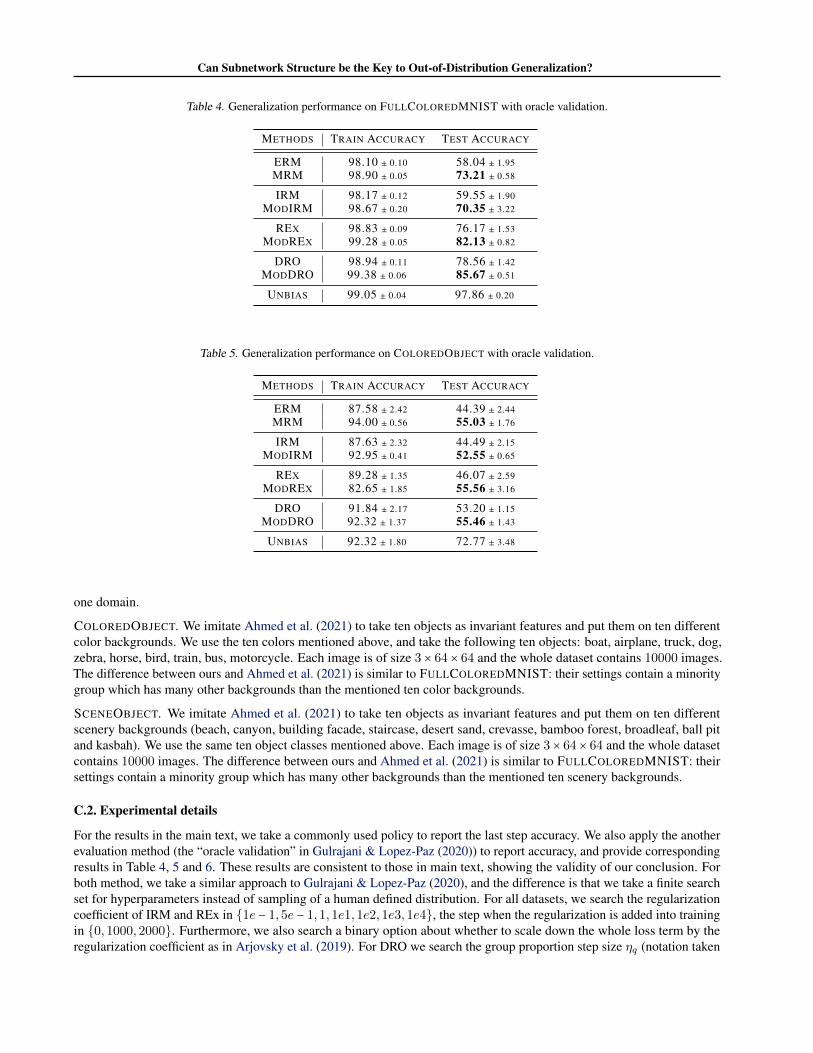
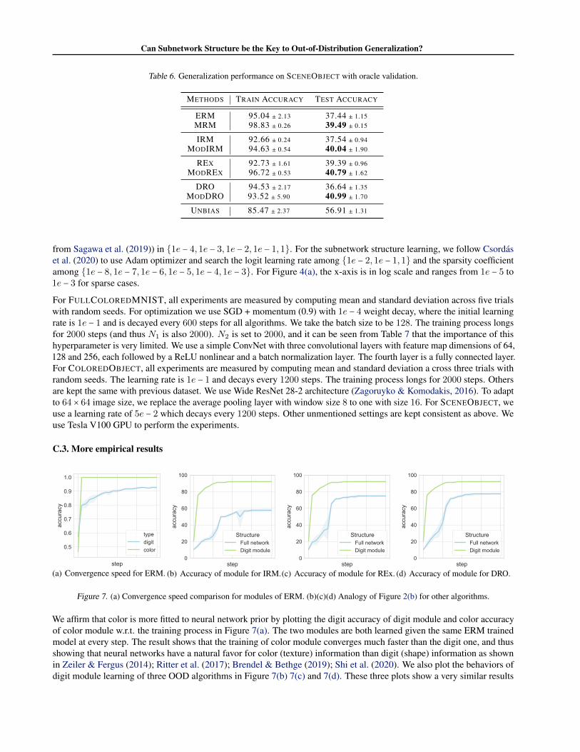
For the results in the main text, we take a commonly used policy to report the last step accuracy. We also apply the anotherevaluation method (the “oracle validation” in Gulrajani & Lopez-Paz (2020)) to report accuracy, and provide correspondingresults in Table 4, 5 and 6. These results are consistent to those in main text, showing the validity of our conclusion. Forboth method, we take a similar approach to Gulrajani & Lopez-Paz (2020), and the difference is that we take a finite searchset for hyperparameters instead of sampling of a human defined distribution. For all datasets, we search the regularizationcoefficient of IRM and REx in {1e − 1,5e − 1,1,1e1,1e2,1e3,1e4}, the step when the regularization is added into trainingin {0,1000,2000}. Furthermore, we also search a binary option about whether to scale down the whole loss term by theregularization coefficient as in Arjovsky et al. (2019). For DRO we search the group proportion step size ηq (notation taken


Table 6. Generalization performance on SCENEOBJECT with oracle validation.


ERM 95.04 ± 2.13 37.44 ± 1.15MRM 98.83 ± 0.26 39.49 ± 0.15

IRM 92.66 ± 0.24 37.54 ± 0.94MODIRM 94.63 ± 0.54 40.04 ± 1.90

REX 92.73 ± 1.61 39.39 ± 0.96MODREX 96.72 ± 0.53 40.79 ± 1.62

DRO 94.53 ± 2.17 36.64 ± 1.35MODDRO 93.52 ± 5.90 40.99 ± 1.70

UNBIAS 85.47 ± 2.37 56.91 ± 1.31

from Sagawa et al. (2019)) in {1e − 4,1e − 3,1e − 2,1e − 1,1}. For the subnetwork structure learning, we follow Csordaset al. (2020) to use Adam optimizer and search the logit learning rate among {1e − 2,1e − 1,1} and the sparsity coefficientamong {1e − 8,1e − 7,1e − 6,1e − 5,1e − 4,1e − 3}. For Figure 4(a), the x-axis is in log scale and ranges from 1e − 5 to1e − 3 for sparse cases.

For FULLCOLOREDMNIST, all experiments are measured by computing mean and standard deviation across five trialswith random seeds. For optimization we use SGD + momentum (0.9) with 1e − 4 weight decay, where the initial learningrate is 1e − 1 and is decayed every 600 steps for all algorithms. We take the batch size to be 128. The training process longsfor 2000 steps (and thus N1 is also 2000). N2 is set to 2000, and it can be seen from Table 7 that the importance of thishyperparameter is very limited. We use a simple ConvNet with three convolutional layers with feature map dimensions of 64,128 and 256, each followed by a ReLU nonlinear and a batch normalization layer. The fourth layer is a fully connected layer.For COLOREDOBJECT, all experiments are measured by computing mean and standard deviation a cross three trials withrandom seeds. The learning rate is 1e − 1 and decays every 1200 steps. The training process longs for 2000 steps. Othersare kept the same with previous dataset. We use Wide ResNet 28-2 architecture (Zagoruyko & Komodakis, 2016). To adaptto 64 × 64 image size, we replace the average pooling layer with window size 8 to one with size 16. For SCENEOBJECT, weuse a learning rate of 5e − 2 which decays every 1200 steps. Other unmentioned settings are kept consistent as above. Weuse Tesla V100 GPU to perform the experiments.

C.3. More empirical results

step

0.5

0.6

0.7

0.8

0.9

1.0

accu

racy

typedigitcolor

(a) Convergence speed for ERM.step

0

20

40

60

80

100

accu

racy


(b) Accuracy of module for IRM.step

0

20

40

60

80

100

accu

racy


(c) Accuracy of module for REx.step

0

20

40

60

80

100

accu

racy


(d) Accuracy of module for DRO.

Figure 7. (a) Convergence speed comparison for modules of ERM. (b)(c)(d) Analogy of Figure 2(b) for other algorithms.

We affirm that color is more fitted to neural network prior by plotting the digit accuracy of digit module and color accuracyof color module w.r.t. the training process in Figure 7(a). The two modules are both learned given the same ERM trainedmodel at every step. The result shows that the training of color module converges much faster than the digit one, and thusshowing that neural networks have a natural favor for color (texture) information than digit (shape) information as shownin Zeiler & Fergus (2014); Ritter et al. (2017); Brendel & Bethge (2019); Shi et al. (2020). We also plot the behaviors ofdigit module learning of three OOD algorithms in Figure 7(b) 7(c) and 7(d). These three plots show a very similar results


step0.0

0.2

0.4

0.6

0.8

1.0

accu

racy

AlgorithmERMIRMRExDRO

(a) Intersection, digit accuracy.step

0.0

0.2

0.4

0.6

0.8

1.0

accu

racy

(b) Intersection, color accuracy.step

0.0

0.2

0.4

0.6

0.8

1.0

accu

racy

(c) Union, digit accuracy.step

0.0

0.2

0.4

0.6

0.8

1.0

accu

racy

(d) Union, color accuracy.

step0.0

0.2

0.4

0.6

0.8

1.0

accu

racy

(e) Complement of intersection,digit accuracy.

step0.0

0.2

0.4

0.6

0.8

1.0

accu

racy

(f) Complement of intersection,color accuracy.

step0.0

0.2

0.4

0.6

0.8

1.0

accu

racy

(g) (Complement of color mod-ule) ∪ (digit module), digit accu-racy.

step0.0

0.2

0.4

0.6

0.8

1.0

accu

racy

(h) (Complement of color mod-ule) ∪ (digit module), color accu-racy.

Figure 8. The digit / color accuracy for some logical operation results of learned digit and color module.

to Figure 2(b). We omit the behavior of color module of these algorithms since it’s very similar to that of ERM shown inFigure 7(a).

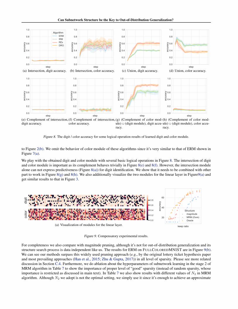
We play with the obtained digit and color module with several basic logical operations in Figure 8. The intersection of digitand color module is important as its complement behaves trivially in Figure 8(e) and 8(f). However, the intersection modulealone can not express predictiveness (Figure 8(a)) for digit identification. We show that it needs to be combined with otherpart to work in Figure 8(g) and 8(h). We also additionally visualize the two modules for the linear layer in Figure9(a) andget similar results to that in Figure 3.

digi

tco

lor

0.0

0.2

0.4

0.6

0.8

(a) Visualization of modules for the linear layer. keep ratio

20

40

60

accu

racy

StructuremagnitudeMRM (Ours)Oracle

Figure 9. Compensatory experimental results.

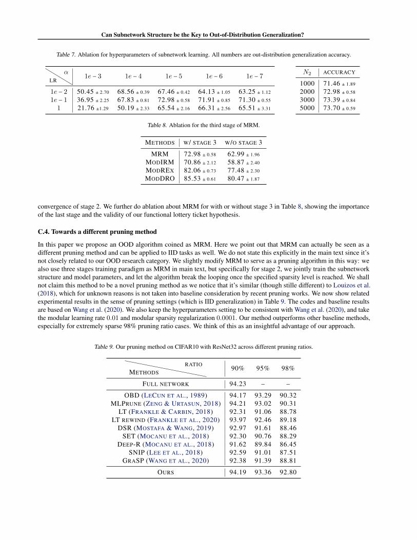
For completeness we also compare with magnitude pruning, although it’s not for out-of-distribution generalization and itsstructure search process is data independent like us. The results for ERM on FULLCOLOREDMNIST are in Figure 9(b).We can see our methods surpass this widely used pruning approach (e.g., by the original lottery ticket hypothesis paperand most prevailing approaches (Han et al., 2015; Zhu & Gupta, 2017)) in all level of sparsity. Please see more relateddiscussion in Section C.4. Furthermore, we do ablation about the hyperparameters of subnetwork learning in the stage 2 ofMRM algorithm in Table 7 to show the importance of proper level of “good” sparsity (instead of random sparsity, whoseimportance is restricted as discussed in main text). In Table 7 we also show results with different values of N2 in MRMalgorithm. Although N2 we adopt is not the optimal setting, we simply use it since it’s enough to achieve an approximate


Table 7. Ablation for hyperparameters of subnetwork learning. All numbers are out-distribution generalization accuracy.

LRα

1e − 3 1e − 4 1e − 5 1e − 6 1e − 7

1e − 2 50.45 ± 2.70 68.56 ± 0.39 67.46 ± 0.42 64.13 ± 1.05 63.25 ± 1.12

1e − 1 36.95 ± 2.25 67.83 ± 0.81 72.98 ± 0.58 71.91 ± 0.85 71.30 ± 0.55

1 21.76 ±1.29 50.19 ± 2.33 65.54 ± 2.16 66.31 ± 2.56 65.51 ± 3.31

N2 ACCURACY

1000 71.46 ± 1.89

2000 72.98 ± 0.58

3000 73.39 ± 0.84

5000 73.70 ± 0.59

Table 8. Ablation for the third stage of MRM.

METHODS W/ STAGE 3 W/O STAGE 3

MRM 72.98 ± 0.58 62.99 ± 1.96

MODIRM 70.86 ± 2.12 58.87 ± 2.40

MODREX 82.06 ± 0.73 77.48 ± 2.30

MODDRO 85.53 ± 0.61 80.47 ± 1.87

convergence of stage 2. We further do ablation about MRM for with or without stage 3 in Table 8, showing the importanceof the last stage and the validity of our functional lottery ticket hypothesis.

C.4. Towards a different pruning method

In this paper we propose an OOD algorithm coined as MRM. Here we point out that MRM can actually be seen as adifferent pruning method and can be applied to IID tasks as well. We do not state this explicitly in the main text since it’snot closely related to our OOD research category. We slightly modify MRM to serve as a pruning algorithm in this way: wealso use three stages training paradigm as MRM in main text, but specifically for stage 2, we jointly train the subnetworkstructure and model parameters, and let the algorithm break the looping once the specified sparsity level is reached. We shallnot claim this method to be a novel pruning method as we notice that it’s similar (though stille different) to Louizos et al.(2018), which for unknown reasons is not taken into baseline consideration by recent pruning works. We now show relatedexperimental results in the sense of pruning settings (which is IID generalization) in Table 9. The codes and baseline resultsare based on Wang et al. (2020). We also keep the hyperparameters setting to be consistent with Wang et al. (2020), and takethe modular learning rate 0.01 and modular sparsity regularization 0.0001. Our method outperforms other baseline methods,especially for extremely sparse 98% pruning ratio cases. We think of this as an insightful advantage of our approach.

Table 9. Our pruning method on CIFAR10 with ResNet32 across different pruning ratios.

METHODSRATIO

90% 95% 98%

FULL NETWORK 94.23 – –

OBD (LECUN ET AL., 1989) 94.17 93.29 90.32MLPRUNE (ZENG & URTASUN, 2018) 94.21 93.02 90.31

LT (FRANKLE & CARBIN, 2018) 92.31 91.06 88.78LT REWIND (FRANKLE ET AL., 2020) 93.97 92.46 89.18

DSR (MOSTAFA & WANG, 2019) 92.97 91.61 88.46SET (MOCANU ET AL., 2018) 92.30 90.76 88.29

DEEP-R (MOCANU ET AL., 2018) 91.62 89.84 86.45SNIP (LEE ET AL., 2018) 92.59 91.01 87.51

GRASP (WANG ET AL., 2020) 92.38 91.39 88.81

OURS 94.19 93.36 92.80

can subnetwork structure be the key to out-of-distribution

Documents