canal blocking optimization in restoration of drained

Biogeosciences, 17, 4769–4784, 2020https://doi.org/10.5194/bg-17-4769-2020© Author(s) 2020. This work is distributed underthe Creative Commons Attribution 4.0 License.

Canal blocking optimization in restoration of drained peatlandsIñaki Urzainki1,2, Ari Laurén2, Marjo Palviainen3, Kersti Haahti1, Arif Budiman4, Imam Basuki4,5, Michael Netzer4,and Hannu Hökkä1

1Natural Resources Institute Finland (Luke), Latokartanonkaari 9, 00790 Helsinki, Finland2School of Forest Sciences, Faculty of Science and Forestry, University of Eastern Finland,Joensuu Campus, P.O. Box 111, Yliopistokatu 7, 80101 Joensuu, Finland3Department of Forest Sciences, University of Helsinki, P.O. Box 27, 00014 Helsinki, Finland4Winrock International, 2121 Crystal Drive, Suite 500, Arlington, VA 22202, USA5Center for International Forestry Research (CIFOR), Situ Gede, Sindang Barang, Bogor 16115, Indonesia

Correspondence: Iñaki Urzainki ([email protected])

Received: 8 March 2020 – Discussion started: 6 April 2020Revised: 27 July 2020 – Accepted: 16 August 2020 – Published: 2 October 2020

Abstract. Drained peatlands are one of the main sources ofcarbon dioxide (CO2) emissions globally. Emission reduc-tion and, more generally, ecosystem restoration can be en-hanced by raising the water table using canal or drain blocks.When restoring large areas, the number of blocks becomeslimited by the available resources, which raises the follow-ing question: in which exact positions should a given numberof blocks be placed in order to maximize the water table risethroughout the area? There is neither a simple nor an analyticanswer. The water table response is a complex phenomenonthat depends on several factors, such as the topology of thecanal network, site topography, peat hydraulic properties,vegetation characteristics and meteorological conditions. Wedeveloped a new method to position the canal blocks basedon the combination of a hydrological model and heuristic op-timization algorithms. We simulated 3 d dry downs from awater saturated initial state for different block positions us-ing the Boussinesq equation, and the block configurationsmaximizing water table rise were searched for by means ofgenetic algorithm and simulated annealing. We applied thisapproach to a large drained peatland area (931 km2) in Suma-tra, Indonesia. Our solution consistently outperformed tradi-tional block locating methods, indicating that drained peat-land restoration can be made more effective at the same costby selecting the positions of the blocks using the presentedscheme.

1 Introduction

Peatlands occupy around 3 % of global land area but hold upto one-third (630 Pg) of all carbon (C) held in active terres-trial pools (Page et al., 2011; Page and Baird, 2016; Xu et al.,2018; Le Quéré et al., 2018; Nichols and Peteet, 2019). Inpristine conditions, peatlands typically act as C sinks sincethe input of dead organic matter is usually greater than thebiological decomposition of peat and other organic residues(Reddy and DaLaune, 2008). However, drainage may turnpeatlands into C sources (Minkkinen and Laine, 1998; Hooi-jer et al., 2010; Ojanen et al., 2010; Jauhiainen et al., 2012),and as a consequence drained peatlands are one of the mainsources of CO2 emissions globally. Drainage removes ex-cess water from peat and enhances site productivity, whichis favorable for agriculture and forest production (Päivänenand Hånell, 2012; Evans et al., 2019). Even though drainage-based bioproduction can be economically viable, it has se-vere environmental drawbacks: it increases CO2 emissions(Ojanen et al., 2010; Jauhiainen et al., 2012), the rate of peatsubsidence (Couwenberg et al., 2010; Hooijer et al., 2010;Carlson et al., 2015; Evans et al., 2019), nutrient export towater courses (Nieminen et al., 2017) and fire risk in peat-lands (Usup et al., 2004; Wösten et al., 2008; Page and Hooi-jer, 2016). CO2 emissions have been particularly severe inmanaged tropical peatlands where the annual CO2 emissionhas been as high as 70–90 Mg ha−1 (Hooijer et al., 2010;Jauhiainen et al., 2012). C emissions from tropical peatlandsin Malaysia and Indonesia in 2015 corresponded to 1.6 % of

Published by Copernicus Publications on behalf of the European Geosciences Union.

4770 I. Urzainki et al.: Canal blocking optimization in restoration of drained peatlands

global fossil fuel emissions (Miettinen et al., 2017). Accord-ing to Hooijer et al. (2010), the CO2 emissions from drainedpeatlands in Indonesia range from 290 to 700 Tg yr−1.

Water table depth (WTD) has been found to be the keyvariable controlling CO2 emissions from decomposition intropical peatlands (Hooijer et al., 2010; Jauhiainen et al.,2012; Carlson et al., 2015; Evans et al., 2019). It has beenestimated that raising the WTD from −80 to −40 cm woulddecrease CO2 emissions on average by 50 Mg ha−1 yr−1

(Jauhiainen et al., 2012) and the rate of peat subsidence by1.7 cm yr−1 (Evans et al., 2019). The reason behind the ben-eficial effects is that increasing water content in peat lim-its oxygen (O2) supply for the decomposer organisms andconsequently slows down the rate of aerobic decomposition(Reddy and DaLaune, 2008). Therefore, raising the WTD is apowerful tool for peatland restoration, the aim of which is toestablish a self-sustaining peat ecosystem that accumulatesC.

Studies of canal and ditch blocking in temperate peat-lands describe how WTD rises for peatland restoration havebeen commonly carried out using drain or canal blocks con-structed from surrounding peat material, mineral soil or arti-ficial materials (Ritzema et al., 2014; Armstrong et al., 2009;Parry et al., 2014). As discussed by Parry et al. (2014), theWTD response depends on site topography (Holden et al.,2006), block position (Holden, 2005), drain spacing and thehydraulic characteristics of peat (Dunn and Mackay, 1996).When restoring large peatland areas, the number of blocksbecomes easily limited by available financial resources. Thisis especially important in tropical peatlands, where the canalsare typically large, requiring large structures that increasethe cost of a single block (Armstrong et al., 2009; Ritzemaet al., 2014). Working with limited resources raises a naturalquestion: in which exact positions should a given number ofblocks be placed in order to maximize the amount of rewet-ted peat and consequently to minimize CO2 emissions andthe rate of subsidence?

To the best of our knowledge there is no systematic ap-proach to support finding optimal block positions (Arm-strong et al., 2009; Ritzema et al., 2014). Experimentallytesting different block positions is impractical and inefficient.Process-based hydrological models, on the other hand, pro-vide a useful tool to reveal changes in the WTD induced bydifferent drainage setups (Dunn and Mackay, 1996). How-ever, for large peatland areas and complex canal networks,process-based models on their own are not sufficient to solvethe best block positions because the number of possible po-sitions becomes subject to a combinatorial explosion. To il-lustrate this, let us consider a setup with b blocks having npossible locations. The number of ways in which the blockscould be arranged equals

(nb

). For the case studied in this pa-

per, the number of possible locations was n= 11311, andb was chosen to range from 0 to 80. To get a grasp of thenumber of possible combinations, let us point out that thereare

(11 311

40)= 1.6×10114 ways to place 40 blocks. Even with

powerful computers it is not feasible to find the best com-bination through an exhaustive search; a different strategy isrequired. By using global optimization methods such as ge-netic algorithm (GA) and simulated annealing (SA), it is pos-sible to find approximate solutions to the problems withoutan exhaustive search. Choosing canal blocking positions isa combinatorial management problem for which global op-timization methods are particularly suitable (Jin et al., 2016;Laurén et al., 2018; Rao, 2009).

Our objective in this work was to build a computationalscheme based on a simple hydrological model coupled withan optimization algorithm that maximizes the amount ofrewetted peat with a given number of canal blocks. The hy-drological model uses the Boussinesq equation to computeWTD as a two-dimensional surface. Using the WTD – aproxy for the CO2 emissions – as the target variable of theoptimization problem, the optimization algorithms (GA andSA) look for the positions of the blocks that minimize theemissions. This scheme was applied to a drained peatlandarea (931 km2) in Sumatra, Indonesia. Topographical detailsof the peatland areas, as well as rainfall data and physicalpeat properties, were employed in the simulations. The impli-cation for different canal blocking schemes will be discussedin the context of regional greenhouse gas emissions.

2 Material and methods

2.1 Study area

The study area was located in Siak, Riau, Indonesia (Fig. 1).The area has a humid tropical climate; the mean annual tem-perature is 27 ◦C with very small monthly variation. Themean annual precipitation in the area is 2696 mm with therainy season extending from October to April. The rainfall ofthe wettest month (November) exceeds 300 mm per month,while the driest month (July) receives 120 mm of rainfall. Ac-cording to long-term weather statistics, the mean dry periodbetween the rainfall events during the dry season is 3.2 d, andthe maximum number of consecutive dry days is 20 (datafrom Pekanbaru airport, located in the same province as thetarget area, years 1994–2013). Because of the humid climateand its topography, the area is characterized by tropical peat-lands; the total area is 1100 km2, of which peatlands cover931 km2. The depth of the peat deposit ranges from 2 to 8 m,the deepest peat deposit being located in the middle of thearea (see Fig. 2). Approximately 30 % of the peat area rep-resents hemic or moderately decomposed peat, and 60 % issapric or highly decomposed peat. The area was drained us-ing canals about 5 to 8 m meters wide, which are also usedfor the transportation of wood and other products. The widestcanals are captured in our dataset, but smaller field drains ex-ist that were omitted in this study due to the coarse resolu-tion of the rasters. The total length of the canal network is

Biogeosciences, 17, 4769–4784, 2020 https://doi.org/10.5194/bg-17-4769-2020

I. Urzainki et al.: Canal blocking optimization in restoration of drained peatlands 4771

1100 km. Typically, the canals are spaced in intervals of 500to 1000 m.

For our computations we used the 100m× 100m resolu-tion raster data shown in Fig. 2, which together describe thesurface elevation (DEM) (Vernimmen et al., 2019), the canallocation, and the peat depth and type. The DEM was pre-processed using the fill sinks algorithm in QGIS 3.4 in orderto identify and fill unwanted surface depressions. The peattype influences the peat physical properties (specific yield,Sy , and transmissivity, T ) of the hydrological simulation, andthe peat thickness of Fig. 2c defines ib, which is the depth ofthe impermeable bottom below the peat surface.

2.2 Computational scheme

The computation consists of the following modules: the canalwater level subroutine, the hydrological model and an op-timization algorithm. Figure 3 describes a single iterationin the optimization process. The canal water level subrou-tine computes the canal water level (CWL) that would re-sult from building canal blocks in some given positions. TheCWL is passed to the peat hydrological model, which solvesthe WTD for the whole area. WTD is closely related to thetarget variable of the optimization problem, 〈ζ 〉, defined inSect. 2.2.2. The optimization algorithm evaluates the targetvariable and decides what canal block configuration will bestudied next. This starts a new iteration. We made use of twooptimization algorithms: genetic algorithm (GA) and simu-lated annealing (SA). We also tested an alternative, simpleroptimization approach (SO) that maximizes the change inCWL instead (see Eq. 13) and bypasses the hydrological sim-ulation completely. See Table 1 for definitions of symbolsused.

2.2.1 Canal water level subroutine

This subroutine calculates the CWL (v′) after building a setof blocks at positions k based on the original CWL (v). In theabsence of any blocks, the CWL is assumed to be at a fixeddistance, w, below the elevation derived from the DEM:

vi = DEMi−w. (1)

Here i ranges over the set of pixels of the DEM that form thecanal network, henceforth called canal raster. In our simu-lations, the value of w was determined by direct observationon site and was set to w = 1.2m.

In order to compute how v would be affected by buildinga block in any pixel of the canal raster, information aboutthe topology of the canal network is needed. In particular, itis necessary to know the direction of water flow to determinewhich adjacent pixels are upstream (and therefore potentiallyaffected by the block). The direction of the water flow was in-ferred from the canal raster following two simple rules. Forany two pixels in the canal network raster, we say that pixel

B is a contiguous upstream pixel of A if and only if the fol-lowing are satisfied:

1. A and B are adjacent to each other (diagonal adjacencyis also allowed);

2. the water level of A is lower than that of B, i.e., vA <vB .

When a block is built in a given pixel of the canal raster, itswater level and the water level of upstream pixels rise up tomatch the height of the block with no delay. In what follows,instead of using the block height as a variable, we use theblock head level (hl). The block head level is defined as thedistance from the DEM elevation to the highest point of theblock (Fig. 4).

A detailed description of the algorithm used to implementthese rules and compute v′ is presented in Appendix A. Thegeneral response of the CWL to a block is schematicallyshown in Fig. 4.

2.2.2 Peat hydrological model

The peat hydrological model simulates the two-dimensionalWTD surface for a given configuration of the blocks. Fromthere it computes the target variable of the optimization al-gorithm, 〈ζ 〉, defined in Eq. (7). The WTD was solved usingthe Boussinesq equation, a quasi-three-dimensional ground-water flow partial differential equation (PDE) which is com-putationally much more efficient than solving the full three-dimensional problem and is a standard groundwater mod-eling equation for domains much wider than they are thick(Bear, 1979; Connorton, 1985; Skaggs, 1980; Koivusaloet al., 2000; Cobb et al., 2017):

Sy(h)∂h

∂t=∂

∂x

(T (h)

∂h

∂x

)+∂

∂y

(T (h)

∂h

∂y

)+P−ET, (2)

where Sy is the specific yield, T is the transmissivity(m2 d−1), h is the hydraulic head (m) and P −ET is thedifference between the precipitation and evapotranspiration(m d−1). The WTD is related to h as follows:

WTD(x,y)=−[s(x,y)−h(x,y)

], (3)

where s is the peat surface in meters above sea level. Equa-tion (2) was numerically solved on a horizontal grid with adaily time step using a finite volume solver (Guyer et al.,2009). Since Eq. (2) is a nonlinear PDE, its solution at eachtime step was found iteratively so as to ensure numerical sta-bility. The number of these internal iterations was set to three,which was regarded as a good compromise between accu-racy and efficiency. The numerical scheme was fully implicitin time for h and explicit for T (h) and Sy(h). The exteriorfaces of the grid were open water bodies, and Dirichlet – con-stant head – boundary conditions were applied on them. Thevalue of h at the canal pixels was forced to be equal to v′ by

https://doi.org/10.5194/bg-17-4769-2020 Biogeosciences, 17, 4769–4784, 2020


Figure 1. (a) Map of Sumatra, Indonesia, with the study area shown in gray. (b) Detailed view of the study area. Map data: © Google, MaxarTechnologies.

Table 1. Terms and symbols used in the study.

Definition Symbol Units Values/ref.

Simulated annealing SAGenetic algorithm GASimple optimization SODigital elevation model DEMPeatland area A m2 9.31× 108

Elevation of the peat surface s m From DEMCanal water level measured from the sea level CWL mVector representation of the CWL v

CWL after building a set of blocks v′

Number of pixels in the canal raster n 11 311Canal block Boolean vector k Eq. (10)Number of blocks b 0. . .80Block head level: distance from peat surface to the highest point of the block hl m 0.2, 0.4Distance between DEM and CWL in the absence of any blocks w m 1.2Water table depth measured from the soil surface (negative downwards) WTD mSpatial average of WTD ζ m Eq. (5)Temporal average of WTD over 3 d 〈ζ 〉 m Eq. (7)Hydraulic head h mPrecipitation P mm d−1 0Evapotranspiration ET mm d−1 3Impermeable bottom: depth of the peat deposit ib m From peat depth rasterSpecific yield Sy

Hydraulic conductivity K m d−1

Transmissivity T m2 d−1 Eq. (4)Marginal benefit MB m3 Eq. (17)



Figure 2. (a) DEM (colored) with the canal network superposed(white), (b) peat types and (c) peat depth. The resolution of therasters is 100m× 100m.

Figure 3. Schematic representation of a single iteration of the com-putation showing the most relevant input and output and the inter-action between the modules. The numbers in parentheses refer tothe corresponding section in the main text. DEM stands for digitalelevation model. The optimization algorithm proposes a particularposition for the canal blocks, k. Then, the canal water level sub-routine computes the canal water level (CWL) resulting from thatblock placement, v′. This information is passed on to the peat hy-drological model, which solves for the WTD with v′ as boundaryconditions and computes the resulting target variable, which is theaverage WTD over 3 dry days, 〈ζ 〉, defined in Sect. 2.2.2. The op-timization algorithm evaluates the performance and proposes a newk according to some rules specific to each algorithm. When usingthe alternative simple optimization strategy (SO), the CWL change,which depends only on v and v′ (see Eq. 13), is used as a target vari-able. This corresponds to the shortcut shown by the dashed arrows.

adding a source term large enough to completely dominatethe corresponding term of the discretized equation (Versteegand Malalasekera, 2007).

In this setup, the transmissivity is given by

T (h)=

h(x,y)∫ib(x,y)

K(x,y,z)dz, (4)

Figure 4. Side view of a canal. The solid blue and the brown hori-zontal lines represent the initial CWL, v, and the height of the peatsurface, s, respectively. The parameter w denotes the distance fromthe peat surface to the CWL. Each pixel is represented by one linesegment. The vertical black line represents the block, and the dot-ted blue line represents the CWL after the block has been placed,v′. The shaded blue area represents the change in the CWL due tothe block. The value of the vector k is ki = 1 if there is a block inpixel i and otherwise ki = 0.

where K is the saturated hydraulic conductivity (m d−1) andib is the depth of the impermeable bottom relative to the peatsurface. It follows from Eq. (4) that the transmissivity is afunction of both h and ib. However, since ib is directly in-ferred from peat depth measurements (see Fig. 2), we sim-plify the notation by letting T (h, ib)= T (h). The layeredstructure of the peat deposit, whose hydraulic conductivityK(x,y,z) can vary by orders of magnitude along the verticaldirection, z, is thus taken into account in T (h). Since pub-lished hydraulic property profiles in tropical peat deposits arescarce (Baird et al., 2017), we parameterized the model basedon the following.

– The degree of decomposition (hemic, sapric) affects thehydraulic conductivity. Hydraulic conductivity valuesfor different decomposition stages were adopted fromWösten et al. (2008).

– Hydraulic conductivity decreases exponentially withdepth (Koivusalo et al., 2000; Cobb et al., 2017).

– Woody peat is the dominant material in tropical peat de-posits. The van Genuchten function was used to com-pute the volumetric water content of peat at depth zfor each degree of decomposition and h. In the absenceof measured tropical peat water retention characteris-tics, we used values from boreal woody peats with thesame peat type and degree of decomposition (Päivänen,1973). From the volumetric water content curves, thespecific yield, Sy , which is the amount of water requiredfor a differential increment in WTD elevation, was cal-culated.

Derived T (h) and S(h) curves for the deepest substrate(10 m) hemic peat are shown in Fig. 5d.

Ponding water in fully saturated profiles was neglected,and all surface water was removed from the computation,



Figure 5. Cross section of the simulated WTD for 3 consecutive dry days after a big rainfall event and peat hydraulic properties. (a) DEM(colored) with the canal network superposed (white) and a straight horizontal blue line indicating the location of the cross section shown inpanels (b) and (c). (b) Peat surface (brown) and cross-sectional view of the WTD (blue) measured in meters above sea level. The multipleblue lines correspond to the WTD for the 3 consecutive days of dry down. Abrupt low peat surface values correspond to canals. The dashedrectangle shows the region magnified in the panel below. (c) Magnified area from the panel above. (d) Transmissivity, T (h), and specificyield, Sy(h), functions for the deepest substrate (10 m) hemic peat.

therefore assuming that the typical runoff velocity of wateris greater than the infiltration velocity.

All simulations started from a fully saturated landscape,i.e., WTD= 0.0m or, equivalently, h= s, which may occurafter a heavy tropical rainfall event. Thereafter, for the op-timization procedure, 3 dry days without any precipitation,P = 0mmd−1 and ET= 3mmd−1, were simulated with adaily time step. The reason to adopt this particular setup isthat the wet initial state acts as a system reset which, if fol-lowed by a period without precipitation, allows for a qualita-tive comparison with observations. The exact number of drydays was decided according to two criteria. On the one hand,the mean of consecutive rainless days during the dry seasonin a 20 yr time window was 3.2 d (data from Pekanbaru air-port, located in the same province as the target area, years1994–2013). On the other hand, three time steps result in amanageable computational load in the optimization process.

The spatially averaged WTD (m) at the end of each timestep, l, was defined as

ζl =1A

∫∫WTD∗l (x,y)dxdy, (5)

where the integral extends to the whole peatland area includ-ing the canals and WTD∗l stands for the solution of Eq. (2) attime step l. The mean WTD over d days is then given by

〈ζ 〉d =1d

d∑l=1

ζl, (6)

where the brackets 〈·〉 denote the temporal average. The av-erage WTD over 3 d is specially relevant in this work, and in

what follows we will denote it without subscripts:

〈ζ 〉 = 〈ζ 〉3. (7)

In order to estimate the annual CO2 emissions that a givenblock configuration produces, the WTD for a full year wasalso simulated. That simulation was also initialized with fullysaturated initial conditions and was made to coincide witha high rainfall event in December 2012. It was assumedthat the yearly emitted amount of CO2 per hectare, mCO2

(Mg ha−1 yr−1), is proportional to 〈ζ 〉365, i.e.,

mCO2 =−α〈ζ 〉365+β, (8)

with coefficients (Jauhiainen et al., 2012)

α = 74.11Mgha−1 m−1 yr−1,

β = 29.34Mgha−1 yr−1. (9)

The exact values of α and β are important for the CO2emission estimation, but they are not relevant for the rest ofthe results produced in this work since only the relative val-ues of mCO2 are of interest in the optimization process. In-stead, the crucial feature is that the annual average WTD islinearly related to the emitted amount of CO2. The wholecomputational scheme is therefore independent of the exactvalues of α and β, and they are only used at the last stage inorder to report the results in units of annual emitted tons ofCO2.

2.2.3 Optimization of block positions

The management question of finding the position of a givennumber of blocks in such a way that the amount of emitted



CO2 or its proxy, 〈ζ 〉, is minimized can be formally formu-lated as follows.

Let k = (k1, . . .,kn) be the Boolean vector indicating thepresence or absence of a block in each canal pixel, i.e.,

ki = 1 if there is a block in position i,

ki = 0 otherwise. (10)

The objective function f : Rn→ R,

f (k)= 〈ζ 〉, (11)

maps a given block setup to 〈ζ 〉, the target variable. The ob-jective function (or, equivalently, the target variable) is to beminimized subject to the constraint that

n∑i

ki = b, (12)

where b is the number of blocks to be built. There is no ana-lytic expression for f . Instead, it is a result of combining thecanal blocking subroutine with the peat hydrological model.As pointed out in the Introduction, the search space is dis-crete and too large for exhaustive search. Moreover, it mighthave many local minima that are not close to the global min-imum, so algorithms that only seek local solutions are notuseful. Therefore, this problem is better addressed with non-linear, global optimization algorithms.

Even global optimization algorithms are not guaranteedto find the optimal solution in a search space in which alloptions cannot be tested. Given that there exists no guar-antee that the process will converge towards the true globalminimum of f , the reliability of the optimization procedurebenefits from exploring more than one optimization method.Genetic algorithm (GA) and simulated annealing (SA) areheuristic methods that can often find the global minimumin many problems and are naturally applicable for the solu-tion of discrete optimization tasks (Rao, 2009). In this case,both algorithms start off with some random k composed of bblocks (b = 0. . .80), for which the resulting 〈ζ 〉 is computed.Then, according to some rules specific to the algorithm, an-other k is proposed. This process is repeated for a fixed num-ber of iterations, the same for all numbers of blocks. Bothalgorithms tend to favor the configurations that result in asmaller value of the target variable, 〈ζ 〉, but they also havethe vital feature of avoiding getting stuck in local minima.In SA, this is achieved by allowing steps that worsen theobjective function with certain probability. This probabilityis controlled by the sole parameter, the temperature (a termcoming from metallurgy, from which the inspiration for itcame), which decreases from an initial maximum value. InGA, on the other hand, the problem is circumvented by eval-uating populations of individual vectors k at each iteration orgeneration. The fittest individuals are passed on to the next it-eration according to some rules that include mixing betweenindividuals, also known as mating, and some randomness, or

mutations. The mutation and the mating probabilities are theonly parameters in the genetic algorithm implementation weused.

The parameters used for both algorithms were fixed bytrial and error, and they are shown in Table 2. The authors areaware that parallel versions of SA exist (see, e.g., de Souzaet al., 2010), but the single processor algorithm was chosenfor this task. GA was run in parallel on 10 processors. Withthe same number of iterations (or generations), paralleliza-tion allows GA to explore 10 times more block configura-tions in a similar amount of time. SA was implemented bymeans of the Python package simanneal 0.5.0 (PyPi, 2019),and for GA the eaSimple algorithm in the DEAP library(Fortin et al., 2012) was used.

This optimization setup is computationally expensive re-gardless of the optimization algorithm used. The main bot-tleneck of the computation is the numerical solution of theBoussinesq equation, Eq. (2). A simpler alternative is to max-imize the CWL change,

CWL change=∑

i∈canal raster

(v′i − vi

), (13)

on its own. The CWL change is represented by the blueshaded area in Fig. 4. The rationale behind this alternativechoice of the target variable is simple: in general, it is to beexpected that a higher CWL will lead to wetter peat through-out the area. By completely bypassing the numerical solutionof the PDE, this approach requires a fraction of the compu-tational resources required for the full optimization proce-dure described above while potentially obtaining a good ap-proximation of the minimum 〈ζ 〉. SO was implemented bymodifying the target variable of GA and was run for 250 000iterations on 10 processors. This amounted to a similar com-putational effort as for the SA and GA algorithms.

To evaluate the performance of the optimization algo-rithms, we compared the resulting 〈ζ 〉 against two other waysof positioning blocks: randomized and rule-based. The ran-dom block configurations were generated by randomly se-lecting locations from a uniform distribution. The value of〈ζ 〉 from 2000 random block configurations was computedand aggregated into the mean, 〈ζ 〉r . The rule-based config-uration was constructed following standard procedure in theabsence of computational tools: blocks were placed in per-pendicular intersections of contour line maps with the canalraster (Ritzema et al., 2014). The rule-based positions of theblocks for b = 10 are shown in Fig. 7a.

In order to enable a meaningful comparison between dif-ferent setups, the average WTD resulting from these simula-tions was normalized with the average WTD in the absenceof blocks, i.e.,

〈ζ (b)〉norm =〈ζ (b)〉

〈ζ (0)〉, (14)

where 〈ζ (b)〉 is the 〈ζ 〉 resulting from placing b blocks.



Table 2. Block locating methods and their parameters. The values of the parameters were decided empirically.

Definition SA GA SO Random Rule-based

Number of iterations or generations 6000 6000 250 000 2000 ManualNumber of processors 1 10 10 1Initial temperature 300Final temperature 1Single point crossover mating prob. 0.3 0.3Mutation probability 0.1 0.1

In a similar vein, we define the improvement of any blocklocating method to be

I (b) = 〈ζ (b)〉− 〈ζ (0)〉. (15)

It measures the simple difference in mean WTD between thereference value, 〈ζ (0)〉, and the one resulting from placing bblocks with any of the methods above. In particular,

I(b)

r = 〈ζ(b)〉r−〈ζ

(0)〉 (16)

will be used to denote the mean improvement achieved bylocating b blocks randomly.

Yet some more insight can be gained by looking at theresults in terms of marginal benefits. We define the marginalbenefit of building b+1b blocks over b blocks to be

MB(b)=

∣∣〈ζ (b+1b)〉norm−〈ζ(b)〉norm

∣∣1b

. (17)

The quantities from Eqs. (14) to (17) are used to investi-gate the performance of all block placing methods in the taskof minimizing 〈ζ 〉 with a fixed number of blocks.

3 Results

3.1 Reality check

In order to demonstrate that the peat hydrological model andthe canal water level subroutine reproduce the expected qual-itative behavior of the WTD, two figures are shown. Figure 5shows the WTD drop during 3 consecutive dry days for across section of the drained area. After 3 dry days, the WTDdrops about 10 cm at the midpoint between two drains sepa-rated by 1.4 km. When the canals are closer to each other, theWTD drop is larger, and if the canals are far enough apart,the peat remains fully saturated. The shape of the WTD solu-tion between two canals is the typical one for diffusion PDEssuch as Eq. (2).

The behavior of the canal water level subroutine is demon-strated by comparing the CWL change in a small drained areawith and without canal blocks (Fig. 6). The effect of the canalblocks on the CWL propagates to different distances depend-ing on local topography. If the slope of v is small, the effect

Figure 6. WTD after 3 dry days with and without blocks. (a) DEM(colored) with the canal network superposed (white) and a rectan-gle indicating the area shown on the right. (b) WTD after 3 drydays without any blocks. (c) WTD after 3 dry days in the same areawith 10 blocks (block locations are indicated by red dots). WTDin the canal raster is defined as v′− s. Blocks help raise the WTDcloser to the surface, but their effectiveness varies depending on thelocal topography.

of a single block can reach distances on the order of a kilo-meter. If, instead, v changes very steeply, the effect of a blockreaches less far. In addition, the amount of rewetted peat as aconsequence of building one block is dependent on the localtopography and physical properties of the peat deposit andon the proximity to other canals. It is precisely the complex-ity of this response that calls for computational methods inorder to solve the optimal block placement.

3.2 Canal block optimization

The average WTD was computed using different scenarioswith an increasing number of canal blocks (b = 5, . . .,80)for each of the block placing methods described (rule-based,random, SA, GA, SO). Their resulting values are shown inFig. 7, and they constitute the main result of the presentstudy.

The most straightforward observation is that the moreblocks there are, the larger the fraction of peat they willrewet, even if they are placed randomly. The second obser-



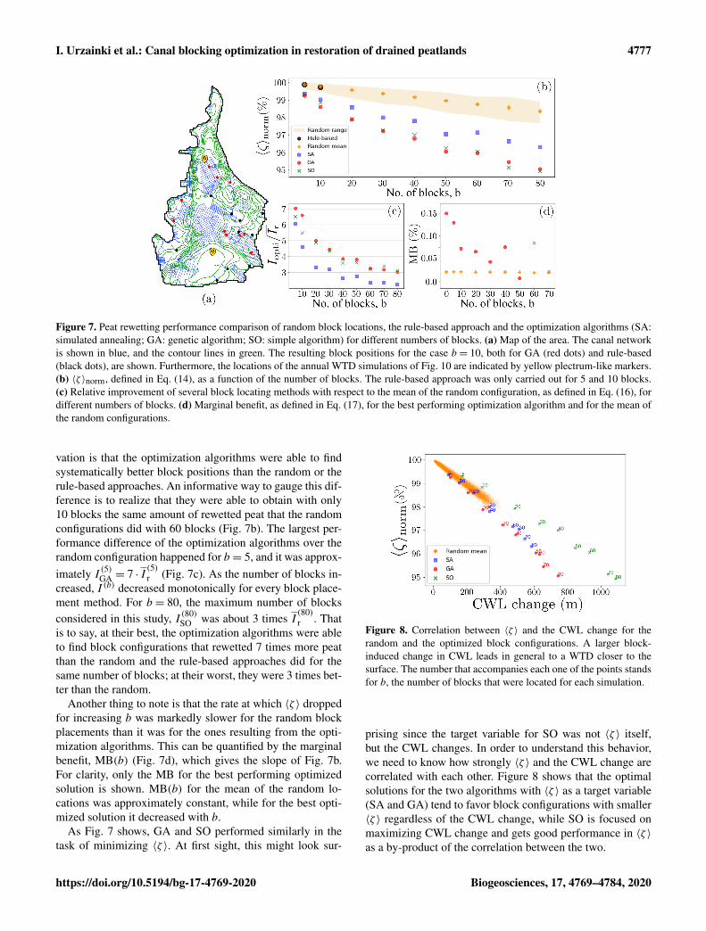
Figure 7. Peat rewetting performance comparison of random block locations, the rule-based approach and the optimization algorithms (SA:simulated annealing; GA: genetic algorithm; SO: simple algorithm) for different numbers of blocks. (a) Map of the area. The canal networkis shown in blue, and the contour lines in green. The resulting block positions for the case b = 10, both for GA (red dots) and rule-based(black dots), are shown. Furthermore, the locations of the annual WTD simulations of Fig. 10 are indicated by yellow plectrum-like markers.(b) 〈ζ 〉norm, defined in Eq. (14), as a function of the number of blocks. The rule-based approach was only carried out for 5 and 10 blocks.(c) Relative improvement of several block locating methods with respect to the mean of the random configuration, as defined in Eq. (16), fordifferent numbers of blocks. (d) Marginal benefit, as defined in Eq. (17), for the best performing optimization algorithm and for the mean ofthe random configurations.

vation is that the optimization algorithms were able to findsystematically better block positions than the random or therule-based approaches. An informative way to gauge this dif-ference is to realize that they were able to obtain with only10 blocks the same amount of rewetted peat that the randomconfigurations did with 60 blocks (Fig. 7b). The largest per-formance difference of the optimization algorithms over therandom configuration happened for b = 5, and it was approx-imately I (5)GA = 7 · I

(5)r (Fig. 7c). As the number of blocks in-

creased, I (b) decreased monotonically for every block place-ment method. For b = 80, the maximum number of blocksconsidered in this study, I (80)

SO was about 3 times I(80)r . That

is to say, at their best, the optimization algorithms were ableto find block configurations that rewetted 7 times more peatthan the random and the rule-based approaches did for thesame number of blocks; at their worst, they were 3 times bet-ter than the random.

Another thing to note is that the rate at which 〈ζ 〉 droppedfor increasing b was markedly slower for the random blockplacements than it was for the ones resulting from the opti-mization algorithms. This can be quantified by the marginalbenefit, MB(b) (Fig. 7d), which gives the slope of Fig. 7b.For clarity, only the MB for the best performing optimizedsolution is shown. MB(b) for the mean of the random lo-cations was approximately constant, while for the best opti-mized solution it decreased with b.

As Fig. 7 shows, GA and SO performed similarly in thetask of minimizing 〈ζ 〉. At first sight, this might look sur-

Figure 8. Correlation between 〈ζ 〉 and the CWL change for therandom and the optimized block configurations. A larger block-induced change in CWL leads in general to a WTD closer to thesurface. The number that accompanies each one of the points standsfor b, the number of blocks that were located for each simulation.

prising since the target variable for SO was not 〈ζ 〉 itself,but the CWL changes. In order to understand this behavior,we need to know how strongly 〈ζ 〉 and the CWL change arecorrelated with each other. Figure 8 shows that the optimalsolutions for the two algorithms with 〈ζ 〉 as a target variable(SA and GA) tend to favor block configurations with smaller〈ζ 〉 regardless of the CWL change, while SO is focused onmaximizing CWL change and gets good performance in 〈ζ 〉as a by-product of the correlation between the two.



Figure 9. Sensitivity of the average WTD to a difference in theblock head level, hl. The values of 〈ζ (b)〉norm correspond to theoptimal block positions computed for hl= 0.2m (orange) and hl=0.4 m (blue). The larger the blocks are, the higher the WTD hasrisen.

The sensitivity of 〈ζ 〉 to the block head level, hl, is demon-strated in Fig. 9 in which we plot 〈ζ 〉norm resulting from thebest available block positions for two different values of theblock head level, hl= {0.2m,0.4m}. There can be a signifi-cant difference in the WTD, especially for large b.

3.3 Implication for CO2 emissions

In order to draw further conclusions about the beneficial en-vironmental impact of building canal blocks, we simulatedthe WTD for a full year under two different regimes: withoutany blocks and with the best available positions for the max-imum number of blocks (80). Rainfall intensity was takenfrom Pekanbaru airport’s weather station data, located in thesame province as the target area. The heavy rainfall eventsregistered during December 2012 were used as the startingpoint for the simulation, which was set up with completelysaturated initial conditions. Evapotranspiration was set to3 mm d−1 and the block head level to hl= 0.4 m. For eachof the two block setups, three daily WTD time series wererecorded: the WTD in a drained area in the north, the WTD inthe natural undrained peat dome in the south (Fig. 7a showsthe exact locations) and the spatially averaged WTD over thewhole area, ζ (Fig. 10).

Nearby blocks were able to raise the water table by ap-proximately 20 cm in the chosen drained location. At theother end of the spectrum, the WTD in the natural zone wasnot affected at all. As a result, the effect of the 80 blocks inthe WTD over the whole area, given by ζ , was to raise it onlyby a few centimeters.

We obtained the following annual average values for theentire area: 〈ζ (0)〉365 =−21.45 cm without any blocks and〈ζ (80)

〉365 =−20.08 cm with the 80 best available blocks.In order to translate our results about the simulated an-nual WTD into the amount of emitted CO2, we usedEq. (8). Thus, m(0)CO2

= 45.34 Mg ha−1 yr−1 and m(80)CO2=

44.22 Mg ha−1 yr−1 were obtained for the aforementionedblock configurations.

4 Discussion

4.1 Model evaluation and reality check

To the best of our knowledge, this work introduces the firstfreely available systematic tool that can quantify the rewet-ting performance of different block configurations. It op-erates on all the easily available data (data derived fromweather and geographic information system, GIS) and com-bines them in a scientifically coherent way. It is also designedto be computationally feasible for large areas. Therefore,this tool can potentially be very useful for decision makersin greenhouse gas emission mitigation and drained peatlandrestoration contexts.

The qualitative behavior of the WTD and of the CWL inFigs. 5 and 6 reflects the following expected traits. First ofall, WTD decreases with time as a result of drainage. Sec-ond, the smaller the distance between canals, the more theWTD drops for it was assumed that the system lacks any wa-ter input. In contrast, the WTD might stay close to the surfaceif the canals are far enough apart. Moreover, the effect of aset of blocks in the CWL propagates upstream in the correctway.

In this study, we did not validate the hydrological modelagainst actual field data because there is no extensive, pub-licly available dataset. The aim of the paper was not to test anew hydrological model per se but rather to solve a manage-ment question by applying a preexisting one with parametervalues derived from the literature. We assume that a moreprecise parameterization would not have changed the out-come of the optimization procedure, and thus the qualitativeassessment of the parameters’ fitness was enough to fulfillour principal objective. It might be argued that in the absenceof a quantitative validation, there is a high uncertainty in thesimulated annual WTD of Fig. 10. However, the simulateddaily WTD of Fig. 10 is in the same range and shows similardynamics as those reported earlier for drained peatlands insimilar areas (Jauhiainen et al., 2012; Hooijer et al., 2012;Evans et al., 2019) and for natural peatland forests in theGreater Sunda Islands (Cobb et al., 2017; Evans et al., 2019).Thus, we assume that WTD in Fig. 10 and the consecutiveCO2 emissions, discussed in Sect. 4.3, are plausible. Further-more, we are aware that the hydrological model presentedhere may produce inaccurate estimates. The discretizationerror introduced with a daily time step could be substantial,and the convergence test could be improved, for instance, bystudying the behavior of the solution with smaller time steps.However, accuracy and convergence needed to be sacrificedas a tradeoff against runtime. The hydrological model neededto be simplified just enough so that a meaningful amount ofblock setups could be explored and the management questioncould be successfully tackled.

Some remarks about the assumptions made in the canalwater level subroutine are in order. As explained inSect. 2.2.1, the CWL in the absence of blocks was inferred



Figure 10. Simulated daily WTD for two sites (drained and natural, see Fig. 7 for the exact locations) within the peatland area and theaverage WTD, ζ . The same period (December 2012–December 2013) was simulated without any blocks (green and purple lines) and withthe 80 optimized blocks (orange and red lines). The spatial average ζ for b = {0,80} is shown in orange and green. There was no appreciabledifference in WTD in the undrained area between different block configurations, and the WTD is shown by a single line (blue line). Dailyrainfall intensity is shown as gray vertical lines (data from Pekanbaru airport).

from the DEM using a constant w (see Eq. 1). This impliesthat any local fluctuation in the height of the DEM is directlytransferred to the CWL. Indeed, a CWL derived in this man-ner is not expected to be monotonically decreasing in the di-rection of water flow. This non-monotonic nature of the CWLcan lead to incorrect predictions of the effect a block has onthe CWL. Another source of misrepresentation of the con-nectivity of the CWL comes from the artifact that the reso-lution of the DEM, 100m× 100m, introduces. According tothe rules in Sect. 2.2.1, if two different canals happen to beless than 100 m apart, then rule 1 will erroneously infer thatthose two pixels are contiguous. Moreover, as mentioned inthe description of the study area, there were small field drainsthat were not captured by the raster maps due to their coarseresolution. All these problems could be ameliorated by usinga separate, complete canal network vector layer which con-tains the direction of the water flow. There is yet another classof approximations that were made in Eq. (1). First of all, inreality the distance between the peat surface and the CWL inthe absence of blocks,w, is not constant; it might vary in timedue to seasonality and in space at different heights. It is alsoworth noting that the resulting water profile after building ablock is typically not a perfectly horizontal line, as depictedwith dotted lines in Fig. 4, but an inclined one. Furthermore,we are implicitly neglecting tidal effects which could affectthe water flow direction close to the seashore. All these ap-proximations were either imposed by the quality of the dataor judged to be of secondary importance in the computationof the CWL.

4.2 Canal block optimization

Two basic observations can be drawn from Fig. 7. The first isthat the performance of the rule-based approach is compara-ble to that of the random location of the blocks. The positionsfor the blocks in the rule-based approach were located inperpendicular intersections between contour lines and canals

(Ritzema et al., 2014), as shown in Fig. 7a. Figure 7a makesit apparent that it is very difficult to predict the effect of theblocks on the WTD by using logical reasoning alone: thereare no evident differences between the locations of the blocksplaced according to the rule-based and the GA methods. Therule-based approach was only carried out for 5 and 10 blocks,yet as b increases, so does the complexity of the task, and itis therefore not expected that it would perform any differ-ently from the random method when the amount of blocksincreased. This leads us to conclude that the combination ofthe random trials and the rule-based approach may be inter-preted as the best humanly possible result in the absence ofany computational tools.

The second observation is that the optimization algorithmsperformed systematically better than the random and rule-based approaches. Going into further details, GA and SOwere more successful in minimizing 〈ζ 〉 than SA. Under thesame conditions, GA and SA are expected to perform simi-larly (Rao, 2009), but the single processor nature of SA re-stricted its search space to be 10 and 417 times smaller thanthose of GA and SO, respectively. The optimization perfor-mance of GA and SO was very similar for all numbers ofblocks, but SO performed best for higher numbers of blocks.Both strategies are sound from the hydrological point ofview, but their success in the optimization happens for differ-ent reasons. The good performance of SO can be explainedby two factors. On the one hand, its simplicity allowed it toexplore 42 times more block configurations than GA, thusbeing able to reach a fairly good approximation of the max-imum CWL change even for large b. On the other hand,〈ζ 〉 and the CWL change correlated strongly as is shown inFig. 8, meaning that SO got a good result in 〈ζ 〉 minimiza-tion as a byproduct of CWL change maximization. Anotherway of putting this is that, unlike the CWL change, 〈ζ 〉 getsthe full three-dimensional information about the catchmenttopography and the peat physical properties, but in return theoptimization task is more demanding. This may not be true



for every study area. For instance, in domains with a highspatial heterogeneity in peat physical properties, the correla-tion is expected to be less evident. As the number of blocksto be located, b, increases, the size of the search space doesso as

(nb

)(which has a maximum at around b = n/2). It is

this rapid increase in computational complexity for reason-able numbers of blocks which might explain the better per-formance of SO when the number of blocks is greater. Fol-lowing this line of reasoning, the fact that SO performs betterthan GA only for b = {70,80} leads us to conclude that com-putational resources are limiting the performance of GA atleast at those values of b; i.e., a substantially better perfor-mance of GA is to be expected for high b if the number ofiterations increased. The success of both GA and SO calls foran alternative optimization strategy that would profit fromboth algorithms’ strengths. Such an algorithm could be de-signed so that GA was initialized with several optima fromthe fast SO.

However interesting, comparing the performance of differ-ent algorithms was not the objective of this work. Instead, themain conclusion can be drawn by contrasting the outcome ofthe optimization algorithms with the best humanly availableguesses. With the same number of blocks, the reduction inaverage WTD by the optimized block configuration is sys-tematically greater than the one achieved simply by logicalreasoning (Ritzema et al., 2014; Armstrong et al., 2009). Thiscontrast is most significant for a small number of blocks, forwhich the average WTD reduction resulting from the bestavailable block locations is up to 7 times larger than the onederived from the mean of the random blocks (Fig. 7c). As thenumber of blocks increases, the relative improvement, I , de-creases and so does its derivative, the marginal benefit, MB,for the best available optimized block positions (Fig. 7d).This implies that the benefit of adding one more block de-creases with the number of blocks that are already built. Thisfact is likely due to two main reasons. On the one hand is theaforementioned difficulty for the algorithms to find the op-timal solution in an increasingly larger search space. On theother hand is the fact that the best positions might alreadybe occupied by some of the blocks. Theoretically, there ex-ists a limiting number of blocks at which the finite size ofthe area would make the marginal benefit decrease even withthe absolute best block locations. We suspect that with thecurrent b we were not yet at the limits of the system andthat this finite-size phenomenon will only be relevant forlarger b. In contrast, the marginal benefit of adding one moreblock was almost constant for the random block configura-tion (i.e., the decrease of 〈V (d)r 〉 was linear), which impliesthat if the blocks were to be built randomly, each additionalblock would be equally successful in reducing 〈ζ 〉.

It is not expected that a different choice of parameterswould affect these general observations of the optimizationresults. While different parameterizations will result in a dif-ferent WTD in absolute terms (see, e.g., the case of varyinghl; Fig. 9), the relative differences in WTD between all block

locating methods remain for different choices of parametervalues.

It is also worth mentioning that solving the steady-stateversion of the Boussinesq equation, Eq. (2), was explored asthe way to compute the target variable of the optimization,〈ζ 〉. However, this approach was discarded in favor of thepresented transient equation due to two observations. First,the steady-state solution does not yield a proper descriptionof groundwater behavior. In tropical climates, rainfall is akey driver of hydrological processes, and rainfall intensity ishighly variable in time. Thus forcing the model to run withaverage rainfall and evapotranspiration does not result in asatisfactory model of these systems. Second, since the PDE isnonlinear, the computational time needed to solve the steady-state version was comparable to the time needed to solve thetransient equation.

4.3 Implication for CO2 emissions

The simulated annual CO2 emissions of Sect. 3.3 are withinthe range of the values in the literature for peatlands in thesame region (Hooijer et al., 2012; Evans et al., 2019). Rel-atively speaking, building 80 blocks for the whole 931 km2

area mitigates only 2.24 % of the CO2 emissions. The reasonfor this modest performance might lie in 80 being too fewblocks for such a large area (our method remains applicablefor the placement of a larger number of blocks at the expenseof longer computing times). Let us note that there are ap-proximately 1100 km of canals. When placing 80 blocks, theexpected distance between a pair of blocks is about 14 km.Yet the influence a block has on the CWL spans, in our studyarea, a maximum of 2 km. Let us stretch our results furtherto give a rough estimate of the number of blocks needed inorder to prevent 10 % of the emissions in the study area. Tak-ing the values for 80 blocks as a reference, and assuming that〈ζ (b)〉 decreases linearly with b, 350 blocks would be neededto reach that emission reduction goal. This would correspondto having on average one block every 3 km. Of course, as-suming that 〈ζ (b)〉 decreases linearly with b is only a roughapproximation (Fig. 7 shows the true dependence). This non-linear dependence points to the second reason for the modestperformance of the 80 blocks: there seems to be room forimprovement in our optimization procedure.

On the other hand, looking at the CO2 emissions in ab-solute terms, building 80 blocks prevents the emission of1.01 t ha−1 yr−1 or a total of 94 156 t annually throughout thewhole area. To get a grasp of the magnitude of these num-bers, they are on the order of what 25 000 cars with an annualmileage of 20 000 km would emit.

It is clear that canal blocking raises WTD and therefore de-creases CO2 fluxes in tropical drained peatlands. The currentapplication does not account for methane emissions whichmight increase with rising WTD (Deshmukh et al., 2020;Manning et al., 2019). The optimization problem would haveto be slightly reformulated to account for both negative and



positive responses of C emissions to WTD rise. Yet the ap-proach presented here would remain applicable provided thatthe hydrological model was extended to include a methaneemission subroutine. This is left as a rather interesting openquestion for future work.

4.4 Application to real-life scenarios

When considering the applicability of our method to real-life scenarios, some of its underlying assumptions should bestated clearly. Our method assumes that it is possible to builda block at any given point in the canal raster and that the costof doing so is constant and independent of site properties.Armstrong et al. (2009) carried out a comprehensive study ofseveral drain blocking strategies in blanket peatlands in theUK. It is apparent from their work that the aforementionedassumptions do not hold in most real-life canal blockingscenarios. In particular, Armstrong et al. (2009) recommendbuilding different types of blocks depending on the follow-ing site-specific variables: gradient of the CWL, canal width,peat wetness, peat depth, exposition of underlying mineralsoil and distance to building site. If our method is to havethe desired practical impact, it should be able to accommo-date these points. One way to do so would be to constructa realistic function that would return block cost based on theabove site properties. Indeed, the variables above may be eas-ily translated into economical terms. For instance, a blockbuilt at a point of the CWL where the head gradient is largerequires stable, expensive structures to avoid block failure.Similarly, a remote building site, wide canals and wet con-ditions increase the cost of building a block. Moreover, thebulk of the data needed to construct the block cost functionis already part of the model (peat depth, DEM, WTD). Re-garding the formulation of the optimization problem, blockcost could be introduced simply by changing the constraintequation, Eq. (12); instead of fixing the number of blocks,the block cost could be fixed.

It remains true that choosing the location of a set of blocksfor best performance is a daunting task due to the com-plexity of the response of the water table and even moreso when different types of blocks are considered. Therefore,the specifics of Figs. 7 to 9 may change when several blocktypes are considered, yet it is expected that the general trendwould be similar; human guesses will not perform as wellas optimized block locations. Nevertheless, the block locat-ing method described in this work will never replace expertknowledge. It should rather build upon it in order to have thedesired practical impact. Our approach acknowledges thatexpert knowledge alone might not be enough to solve therewetting problem of drained peatlands in an optimal way,and it opens up the opportunity for local experts and organi-zations to use process-based hydrological modeling and nu-merical optimization techniques, which, as we have hope-fully succeeded to show, can be powerful tools.

5 Conclusions

We constructed an optimization scheme that looks for themaximum water table rise for a drained peatland area givena fixed amount of canal blocks. Our results show that, withthe same amount of resources (i.e., number of blocks),the present computational setup enables a more effectivecanal blocking restoration of drained peatlands than humanguesses do. The computational approach also enables a cost-benefit analysis to solve several management questions.



Appendix A: Canal water level subroutine

The information about the topology of the canal network wasstored in a (sparse) matrix, M, of dimensions (n× n), wheren is the number of pixels in the canal raster. For any twopixels of the canal raster, i and j , the entries of the matrix Mare

Mij = 1 if j is a contiguous upstream pixel of i,

Mij = 0 otherwise. (A1)

Contiguous upstream pixels were defined in rules 1 and 2of Sect. 2.2.1. Note in particular that if MAB = 1, that is, ifpixels A and B are adjacent and pixel B is upstream, it fol-lows that MBA = 0. Moreover, note that Mii = 0 for any i.In other words, M is not symmetrical, and all the elementsof its diagonal are equal to 0. M can then be interpreted asthe adjacency matrix of the simple, directed graph,G, whosenodes are the pixels of the canal raster, and an edge existsif two nodes are in direct physical contact (Newman, 2018).In such a graph, the direction of the edges is the opposite tothe direction of the water flow. Within this setup, the vectork′ = kM, where k is the vector of the blocks’ positions de-fined in Eq. (10), contains the information about all the firstneighbors of the blocks in k. Specifically,

k′j = kiMij = 1 if pixel j is a contiguous upstream

pixel of pixel i,k′j = kiMij = 0 otherwise. (A2)

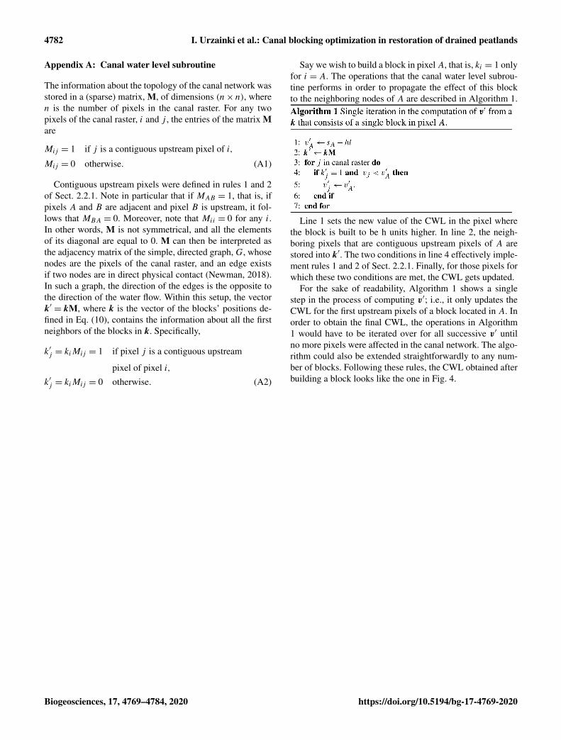
Say we wish to build a block in pixelA, that is, ki = 1 onlyfor i = A. The operations that the canal water level subrou-tine performs in order to propagate the effect of this blockto the neighboring nodes of A are described in Algorithm 1.

Line 1 sets the new value of the CWL in the pixel wherethe block is built to be h units higher. In line 2, the neigh-boring pixels that are contiguous upstream pixels of A arestored into k′. The two conditions in line 4 effectively imple-ment rules 1 and 2 of Sect. 2.2.1. Finally, for those pixels forwhich these two conditions are met, the CWL gets updated.

For the sake of readability, Algorithm 1 shows a singlestep in the process of computing v′; i.e., it only updates theCWL for the first upstream pixels of a block located in A. Inorder to obtain the final CWL, the operations in Algorithm1 would have to be iterated over for all successive v′ untilno more pixels were affected in the canal network. The algo-rithm could also be extended straightforwardly to any num-ber of blocks. Following these rules, the CWL obtained afterbuilding a block looks like the one in Fig. 4.



Code and data availability. The source code and thedata used are available under the MIT license athttps://doi.org/10.5281/zenodo.3741043 (Urzainki and Lau-rén, 2020; https://github.com/LukeEcomod/blopti, last access:6 April 2020).

Author contributions. IU and AL contextualized the problem anddeveloped the model code. IU performed the simulations. AB, IBand MN produced and validated the datasets. KH helped formulatethe research goals and methods. MP, HH and AL contributed byreviewing and editing the paper. IU prepared the paper with contri-butions from all coauthors.

Competing interests. The authors declare that they have no conflictof interest.

Acknowledgements. The authors wish to thank the referees’ thor-ough comments on the paper and Harri Koivusalo for useful dis-cussions about the hydrological modeling. Furthermore, the authorswish to acknowledge CSC – IT Center for Science, Finland, forcomputational resources.

Review statement. This paper was edited by Alexandra Koningsand reviewed by Alex Cobb and one anonymous referee.

References

Armstrong, A., Holden, J., Kay, P., Foulger, M., Gledhill, S., Mc-donald, A. T., and Walker, A.: Drain-blocking techniques onblanket peat: A framework for best practice, J. Environ. Manage.,90, 3512–3519, https://doi.org/10.1016/j.jenvman.2009.06.003,2009.

Baird, A. J., Low, R., Young, D., Swindles, G. T., Lopez, O. R.,and Page, S.: High permeability explains the vulnerability of thecarbon store in drained tropical peatlands, Geophys. Res. Lett.,44, 1333–1339, https://doi.org/10.1002/2016GL072245, 2017.

Bear, J.: Hydraulics of Groundwater, McGraw-Hill Series in WaterResources and Environmental Engineering, McGraw-Hill, NewYork 1979.

Carlson, K. M., Goodman, L. K., and May-Tobin, C. C.: Modelingrelationships between water table depth and peat soil carbon lossin Southeast Asian plantations, Environ. Res. Lett., 10, 074006,https://doi.org/10.1088/1748-9326/10/7/074006, 2015.

Cobb, A. R., Hoyt, A. M., Gandois, L., Eri, J., Dommain, R., Salim,K. A., Kai, F. M., Su’ut, N. S. H., and Harvey, C. F.: How tem-poral patterns in rainfall determine the geomorphology and car-bon fluxes of tropical peatlands, P. Natl. Acad. Sci. USA, 114,E5187–E5196, https://doi.org/10.1073/pnas.1701090114, 2017.

Connorton, B. J.: Does the regional groundwater-flow equa-tion model vertical flow?, J. Hydrol., 79, 279–299,https://doi.org/10.1016/0022-1694(85)90059-9, 1985.

Couwenberg, J., Dommain, R., and Joosten, H.: Greenhousegas fluxes from tropical peatlands in south-east Asia, Glob.

Change Biol., 16, 1715–1732, https://doi.org/10.1111/j.1365-2486.2009.02016.x, 2010.

Deshmukh, C. S., Julius, D., Evans, C. D., Nardi, Susanto,A. P., Page, S. E., Gauci, V., Laurén, A., Sabiham, S., Agus,F., Asyhari, A., Kurnianto, S., Suardiwerianto, Y., and De-sai, A. R.: Inmpact of forest plantation on methane emissionsfrom tropical peatland, Glob. Change Biol., 26, 2477–2495,https://doi.org/10.1111/gcb.15019, 2020.

de Souza, S. X., Suykens, J. A. K., Vandewalle, J., and Bollé, D.:Coupled Simulated Annealing, IEEE T. Syst. Man Cy. B, 40,320–335, 2010.

Dunn, S. and Mackay, R.: Modelling the hydrological im-pacts of open ditch drainage, J. Hydrol., 179, 37–66,https://doi.org/10.1016/0022-1694(95)02871-4, 1996.

Evans, C. D., Williamson, J. M., Kacaribu, F., Irawan, D., Suardi-werianto, Y., Hidayat, M. F., Ari, L., and Page, S. E.: Rates andspatial variability of peat subsidence in Acacia plantation andforest landscapes in Sumatra, Indonesia, Geoderma, 338, 410–421, https://doi.org/10.1016/j.geoderma.2018.12.028, 2019.

Fortin, F.-A., De Rainville, F.-M., Gardner, M.-A., Parizeau, M.,and Gagné, C.: DEAP: Evolutionary Algorithms Made Easy, J.Mach. Learn. Res., 13, 2171–2175, 2012.

Guyer, J. E., Wheeler, D., and Warren, J. A.: FiPy: Partial Differen-tial Equations with Python, Comput. Sci. Eng., 11, 6–15, 2009.

Holden, J.: Peatland hydrology and carbon release: why small-scale process matters, Philos. T. Roy. Soc. A, 363, 2891–2913,https://doi.org/10.1098/rsta.2005.1671, 2005.

Holden, J., Evans, M. G., Burt, T. P., and Horton, M.: Impact of landdrainage on peatland hydrology, J. Environ. Qual., 35, 1764–1778, 2006.

Hooijer, A., Page, S., Canadell, J. G., Silvius, M., Kwadijk, J.,Wösten, H., and Jauhiainen, J.: Current and future CO2 emis-sions from drained peatlands in Southeast Asia, Biogeosciences,7, 1505–1514, https://doi.org/10.5194/bg-7-1505-2010, 2010.

Hooijer, A., Page, S., Jauhiainen, J., Lee, W. A., Lu, X.X., Idris, A., and Anshari, G.: Subsidence and carbon lossin drained tropical peatlands, Biogeosciences, 9, 1053–1071,https://doi.org/10.5194/bg-9-1053-2012, 2012.

Jauhiainen, J., Hooijer, A., and Page, S. E.: Carbon dioxide emis-sions from an Acacia plantation on peatland in Sumatra, Indone-sia, Biogeosciences, 9, 617–630, https://doi.org/10.5194/bg-9-617-2012, 2012.

Jin, X., Pukkala, T., and Li, F.: Fine-tuning heuristic methods forcombinatorial optimization in forest planning, Eur. J. For. Res.,135, 765–779, 2016.

Koivusalo, H., Karvonen, T., and Lepistö, A.: A quasi-three-dimensional model for predicting rainfall-runoff processes in aforested catchment in Southern Finland, Hydrol. Earth Syst. Sci.,4, 65–78, https://doi.org/10.5194/hess-4-65-2000, 2000.

Laurén, A., Asikainen, A., Kinnunen, J.-P., Palviainen, M., andSikanen, L.: Improving the financial performance of solid forestfuel supply using a simple moisture and dry matter loss simula-tion and optimization, Biomass Bioenerg., 116, 72–79, 2018.

Le Quéré, C., Andrew, R. M., Friedlingstein, P., Sitch, S., Hauck,J., Pongratz, J., Pickers, P. A., Korsbakken, J. I., Peters, G. P.,Canadell, J. G., Arneth, A., Arora, V. K., Barbero, L., Bastos,A., Bopp, L., Chevallier, F., Chini, L. P., Ciais, P., Doney, S. C.,Gkritzalis, T., Goll, D. S., Harris, I., Haverd, V., Hoffman, F. M.,Hoppema, M., Houghton, R. A., Hurtt, G., Ilyina, T., Jain, A.


https://doi.org/10.5281/zenodo.3741043

https://github.com/LukeEcomod/blopti

https://doi.org/10.1016/j.jenvman.2009.06.003

https://doi.org/10.1002/2016GL072245

https://doi.org/10.1088/1748-9326/10/7/074006

https://doi.org/10.1073/pnas.1701090114

https://doi.org/10.1016/0022-1694(85)90059-9

https://doi.org/10.1111/j.1365-2486.2009.02016.x

https://doi.org/10.1111/j.1365-2486.2009.02016.x

https://doi.org/10.1111/gcb.15019

https://doi.org/10.1016/0022-1694(95)02871-4

https://doi.org/10.1016/j.geoderma.2018.12.028

https://doi.org/10.1098/rsta.2005.1671

https://doi.org/10.5194/bg-7-1505-2010

https://doi.org/10.5194/bg-9-1053-2012

https://doi.org/10.5194/bg-9-617-2012

https://doi.org/10.5194/bg-9-617-2012

https://doi.org/10.5194/hess-4-65-2000


K., Johannessen, T., Jones, C. D., Kato, E., Keeling, R. F., Gold-ewijk, K. K., Landschützer, P., Lefèvre, N., Lienert, S., Liu, Z.,Lombardozzi, D., Metzl, N., Munro, D. R., Nabel, J. E. M. S.,Nakaoka, S., Neill, C., Olsen, A., Ono, T., Patra, P., Peregon,A., Peters, W., Peylin, P., Pfeil, B., Pierrot, D., Poulter, B., Re-hder, G., Resplandy, L., Robertson, E., Rocher, M., Rödenbeck,C., Schuster, U., Schwinger, J., Séférian, R., Skjelvan, I., Stein-hoff, T., Sutton, A., Tans, P. P., Tian, H., Tilbrook, B., Tubiello,F. N., van der Laan-Luijkx, I. T., van der Werf, G. R., Viovy, N.,Walker, A. P., Wiltshire, A. J., Wright, R., Zaehle, S., and Zheng,B.: Global Carbon Budget 2018, Earth Syst. Sci. Data, 10, 2141–2194, https://doi.org/10.5194/essd-10-2141-2018, 2018.

Manning, F. C., Kho, L. K., Hill, T. C., Cornulier, T., andTeh, Y. A.: Carbon emissions from oil palm plantations onpeat soil, Frontiers in Forests and Global Change, 2, 37 pp.,https://doi.org/10.3389/ffgc.2019.00037, 2019.

Miettinen, J., Hooijer, A., Vernimmen, R., Liew, S. C., and Page,S. E.: From carbon sink to carbon source: extensive peat oxida-tion in insular Southeast Asia since 1990, Environ. Res. Lett., 12,024014, https://doi.org/10.1088/1748-9326/aa5b6f, 2017.

Minkkinen, K. and Laine, J.: Long-term effect of forest drainage onthe peat carbon stores of pine mires in Finland, Can. J. ForestRes., 28, 1267–1275, https://doi.org/10.1139/x98-104, 1998.

Newman, M.: Networks, 2nd Edn., Oxford University Press, NewYork, 2018.

Nichols, J. E. and Peteet, D. M.: Rapid expansion of northern peat-lands and doubled estimate of carbon storage, Nat. Geosci., 12,917–921, https://doi.org/10.1038/s41561-019-0454-z, 2019.

Nieminen, M., Sallantaus, T., Ukonmaanaho, L., and Sarkkola,S.: Nitrogen and phosphorus concentrations in discharge fromdrained peatland forests are increasing, Sci. Total Environ., 609,974–981, https://doi.org/10.1016/j.scitotenv.2017.07.210, 2017.

Ojanen, P., Minkkinen, K., Alm, J., and Penttilä, T.: Soil-atmosphere CO2, CH4 and N2O fluxes in boreal forestry-drained peatlands, Forest Ecol. Manage., 260, 411–421,https://doi.org/10.1016/j.foreco.2010.04.036, 2010.

Page, S. E. and Baird, A. J.: Peatlands and Global Change: Re-sponse and Resilience, Annu. Rev. Env. Resour., 41, 35–57,2016.

Page, S. E. and Hooijer, A.: In the line of fire: the peatlandsof Southeast Asia, Philos. T. Roy. Soc. B, 371, 20150176,https://doi.org/10.1098/rstb.2015.0176, 2016.

Page, S. E., Rieley, J. O., and Banks, C. J.: Global andregional importance of the tropical peatland carbon pool,Glob. Change Biol., 17, 798–818, https://doi.org/10.1111/j.1365-2486.2010.02279.x, 2011.

Päivänen, J.: Hydraulic conductivity and water reten-tion in peat soils, Acta Forestalia Fennica, 129, 7563,https://doi.org/10.14214/aff.7563, 1973.

Päivänen, J. and Hånell, B.: Peatland Ecology and Forestry -ASound Approach, University of Helsinki Department of ForestSciences Publications 3, Helsinki, 2012.

Parry, L. E., Holden, J., and Chapman, P. J.: Restoration of blanketpeatlands, J. Environ. Manage., 133, 193–205, 2014.

PyPi: Simulated Annealing in Python, available at: https://pypi.org/project/simanneal/, last access: 16 December 2019.

Rao, S. S.: Engineering Optimization -Theory and Practice, JohnWiley & Sons, Hoboken, New Jersey, 2009.

Reddy, K. R. and DaLaune, R. D.: Biogeochemistry of Wetlands,CRC Press, Florida, USA, 2008.

Ritzema, H., Limin, S., Kusin, K., Jauhiainen, J., and Wösten,H.: Canal blocking strategies for hydrological restoration ofdegraded tropical peatlands in Central Kalimantan, Indonesia,Catena, 114, 11–20, 2014.

Skaggs, R. W.: A water management model for artificially drainedsoils, Technical Bulletin, North Carolina Agricultural Experi-ment Station, 267, 54 pp., 1980.

Urzainki, I. and Laurén. A.: Blopti – canal blocking optimization,Zenodo, https://doi.org/10.5281/zenodo.3741043, 2020.

Usup, A., Hashimoto, Y., Takahashi, H., and Hayasaka, H.: Com-bustion and thermal characteristics of peat fire in tropicalpeatland in Central Kalimantan, Indonesia, Tropics, 14, 1–9,https://doi.org/10.3759/tropics.14.1, 2004.

Vernimmen, R., Hooijer, A., Yuherdha, A. T., Visser, M., Pronk,M., Eilander, D., Akmalia, R., Fitranatanegara, N., Mulyadi, D.,Andreas, H., Ouellette, J., and Hadley, W.: Creating a Lowlandand Peatland Landscape Digital Terrain Model (DTM) from In-terpolated Partial Coverage LiDAR Data for Central Kaliman-tan and East Sumatra, Indonesia, Remote Sensing, 11, 1152,https://doi.org/10.3390/rs11101152, 2019.

Versteeg, H. K. and Malalasekera, W.: An Introduction to Compu-tational Fluid Dynamics, 2nd Edn., Pearson Education Limited,Harlow, England, 2007.

Wösten, J. H. M., Clymans, E., Page, S. E., Rieley, J. O., and Limin,S. H.: Peat-water interrelationships in a tropical peatland ecosys-tem in Southeast Asia, Catena, 73, 212–224, 2008.

Xu, J., Morris, P. J., Liu, J., and Holden, J.: PEATMAP: Refining es-timates of global peatland distribution based on a meta-analysis,Catena, 160, 134–140, 2018.


https://doi.org/10.5194/essd-10-2141-2018

https://doi.org/10.3389/ffgc.2019.00037

https://doi.org/10.1088/1748-9326/aa5b6f

https://doi.org/10.1139/x98-104

https://doi.org/10.1038/s41561-019-0454-z

https://doi.org/10.1016/j.scitotenv.2017.07.210

https://doi.org/10.1016/j.foreco.2010.04.036

https://doi.org/10.1098/rstb.2015.0176

https://doi.org/10.1111/j.1365-2486.2010.02279.x

https://doi.org/10.1111/j.1365-2486.2010.02279.x

https://doi.org/10.14214/aff.7563

https://pypi.org/project/simanneal/

https://pypi.org/project/simanneal/

https://doi.org/10.5281/zenodo.3741043

https://doi.org/10.3759/tropics.14.1

https://doi.org/10.3390/rs11101152

canal blocking optimization in restoration of drained

Documents