cap 5415: computer vision lecture 2
TRANSCRIPT
CAP 5415: Computer VisionLecture 2
More Linear Processing
Today
• We’ll revisit convolutions and Fourier Transforms
• Today is the day to get a solid understanding
• Don’t let me go on if you don’t understand something
•
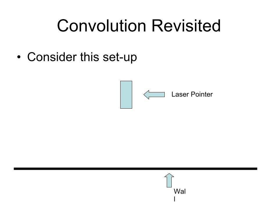
Convolution Revisited
• Consider this set-up
Laser Pointer
Wall
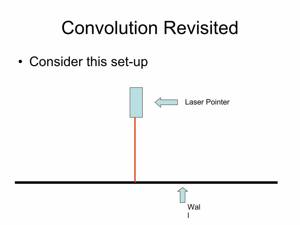
Convolution Revisited
• Consider this set-up
Laser Pointer
Wall
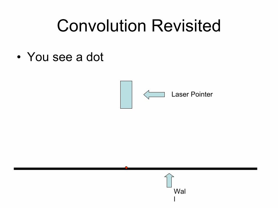
Convolution Revisited
• You see a dot
Laser Pointer
Wall
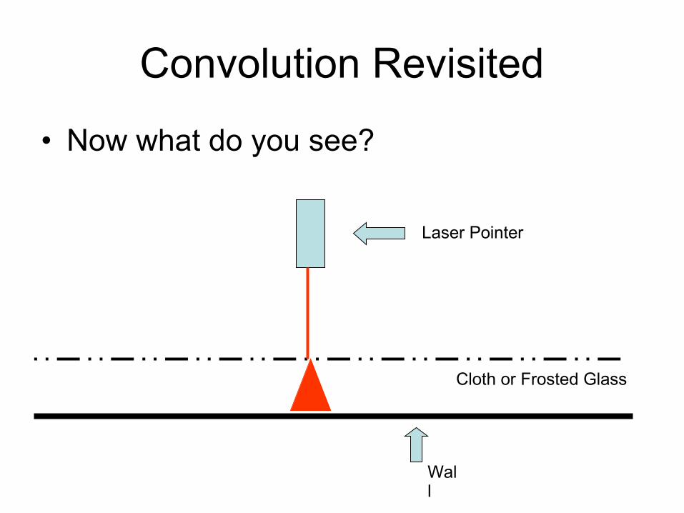
Convolution Revisited
• Now what do you see?
Laser Pointer
Wall
Cloth or Frosted Glass
Kernel
• The kernel is sometimes referred to as a point-spread function
• Relates how an input at one point affects our measurements
• Laser beam -> Frosted Glass -> Blurry dot
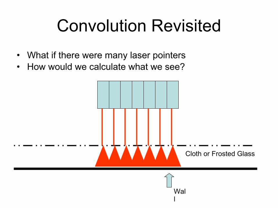
Convolution Revisited
• What if there were many laser pointers• How would we calculate what we see?
Wall
Cloth or Frosted Glass
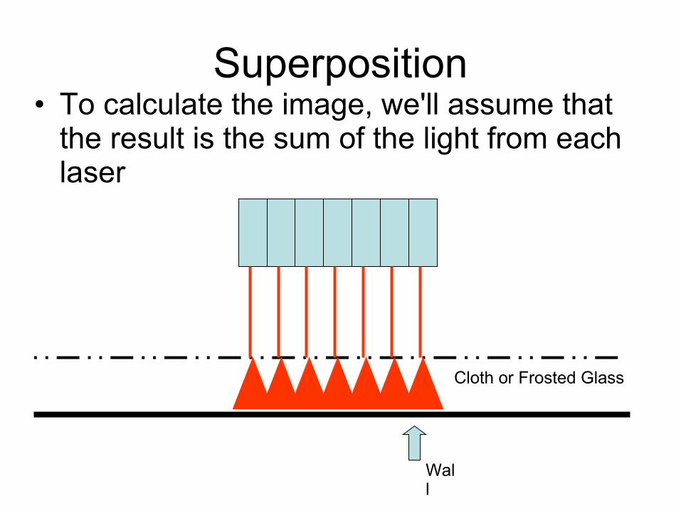
Superposition• To calculate the image, we'll assume that
the result is the sum of the light from each laser
Wall
Cloth or Frosted Glass
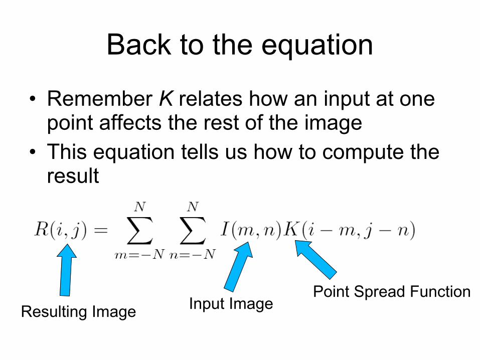
Resulting Image Input ImagePoint Spread Function
Back to the equation
• Remember K relates how an input at one point affects the rest of the image
• This equation tells us how to compute the result
Practical Example
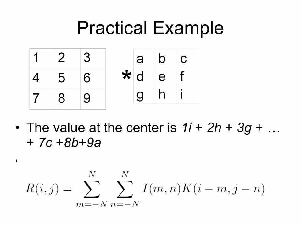
• The value at the center is 1i + 2h + 3g + … + 7c +8b+9a
•
1 2 3
4 5 6
7 8 9
a b cd e fg h i*
Convolution
• We’re focusing on the case where the system is represented by a kernel
• Any questions?
More General Linear Transformations
• Now that we can filter images, is there a good way to analyze what the filtering is doing?
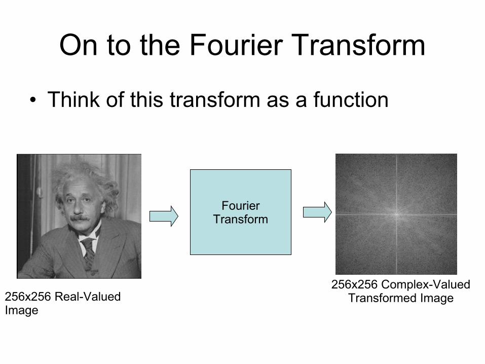
On to the Fourier Transform
• Think of this transform as a function
Fourier Transform
256x256 Real-Valued Image
256x256 Complex-Valued Transformed Image
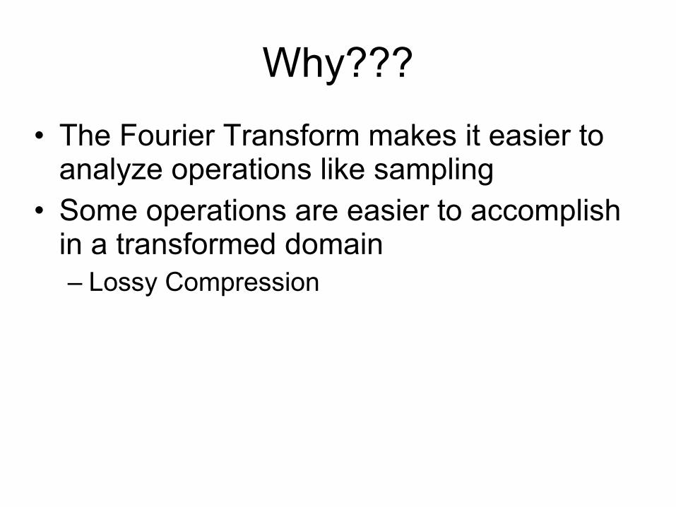
Why???
• The Fourier Transform makes it easier to analyze operations like sampling
• Some operations are easier to accomplish in a transformed domain– Lossy Compression
A simple example of the value of transformations
• Let's consider some simple data• (Handout)
A Short Linear Algebra Review
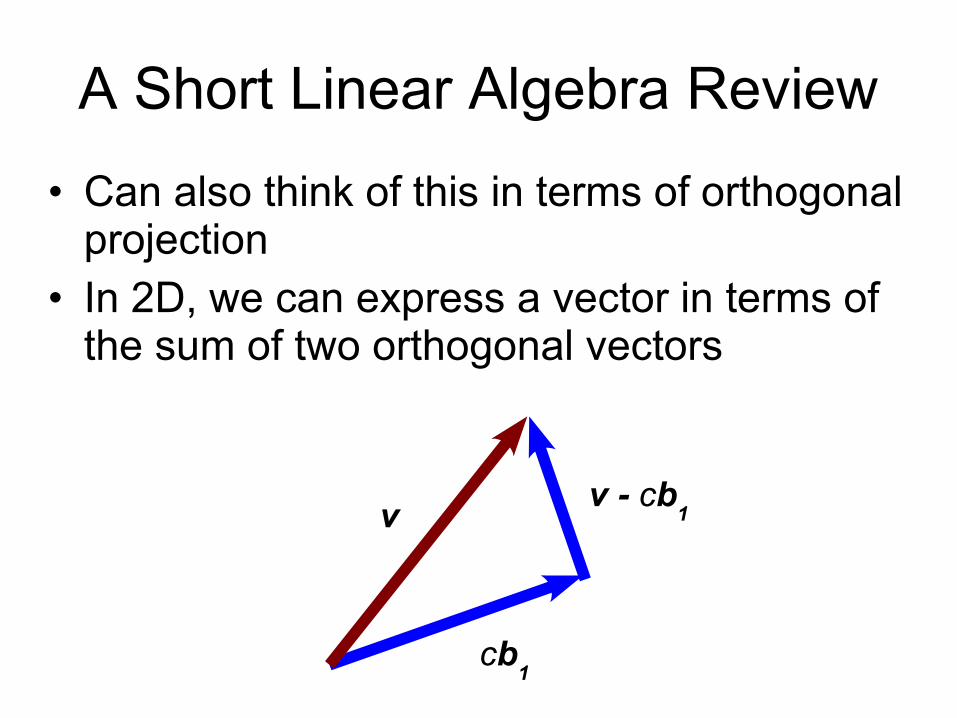
• Can also think of this in terms of orthogonal projection
• In 2D, we can express a vector in terms of the sum of two orthogonal vectors
v - cb1
cb1
v
A Short Linear Algebra Review
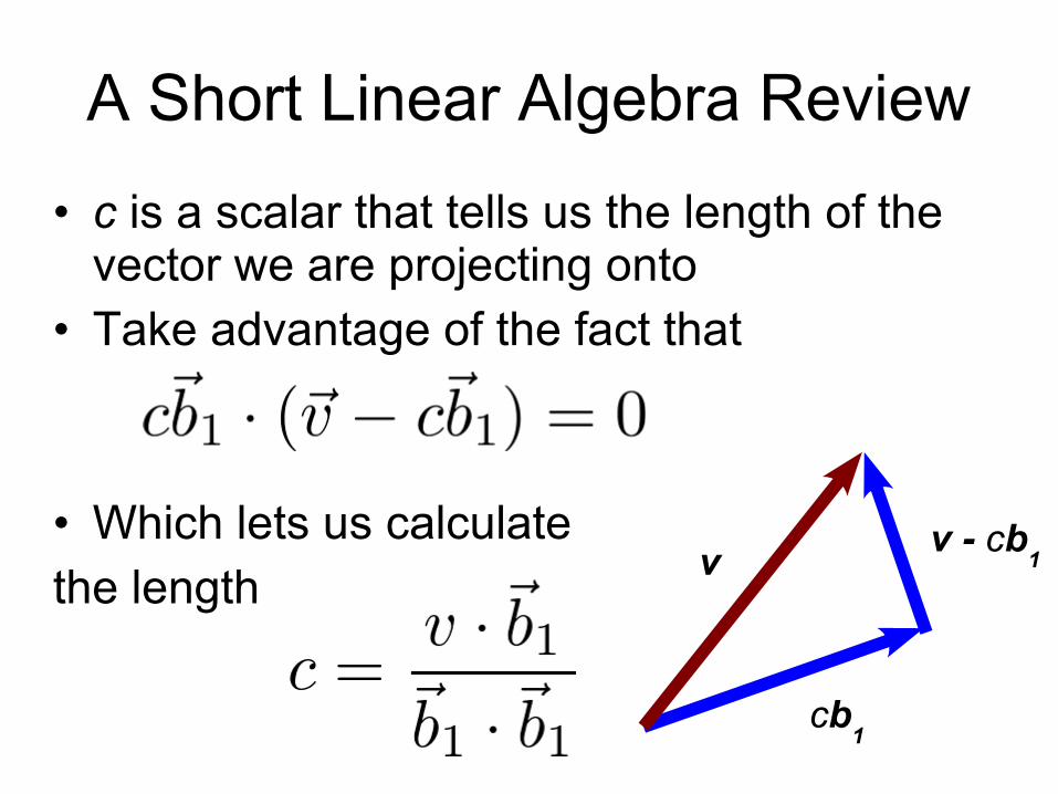
• c is a scalar that tells us the length of the vector we are projecting onto
• Take advantage of the fact that
• Which lets us calculate the length
v - cb1
cb1
v
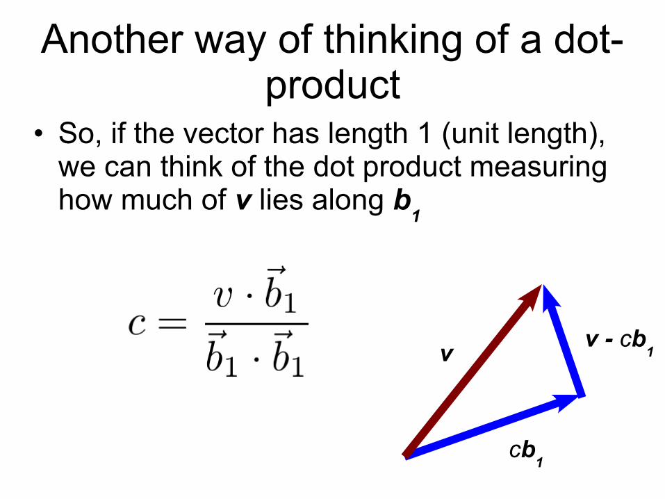
Another way of thinking of a dot-product
• So, if the vector has length 1 (unit length), we can think of the dot product measuring how much of v lies along b
1
v - cb1
cb1
v
Links to the Fourier Transform
• The handout examined points in 2D• We can think of images as points in N-D
– Raster-scan images into a vector
• The Fourier Transform will essentially re-project the image onto a new basis
• Will give a different way of looking at the image.
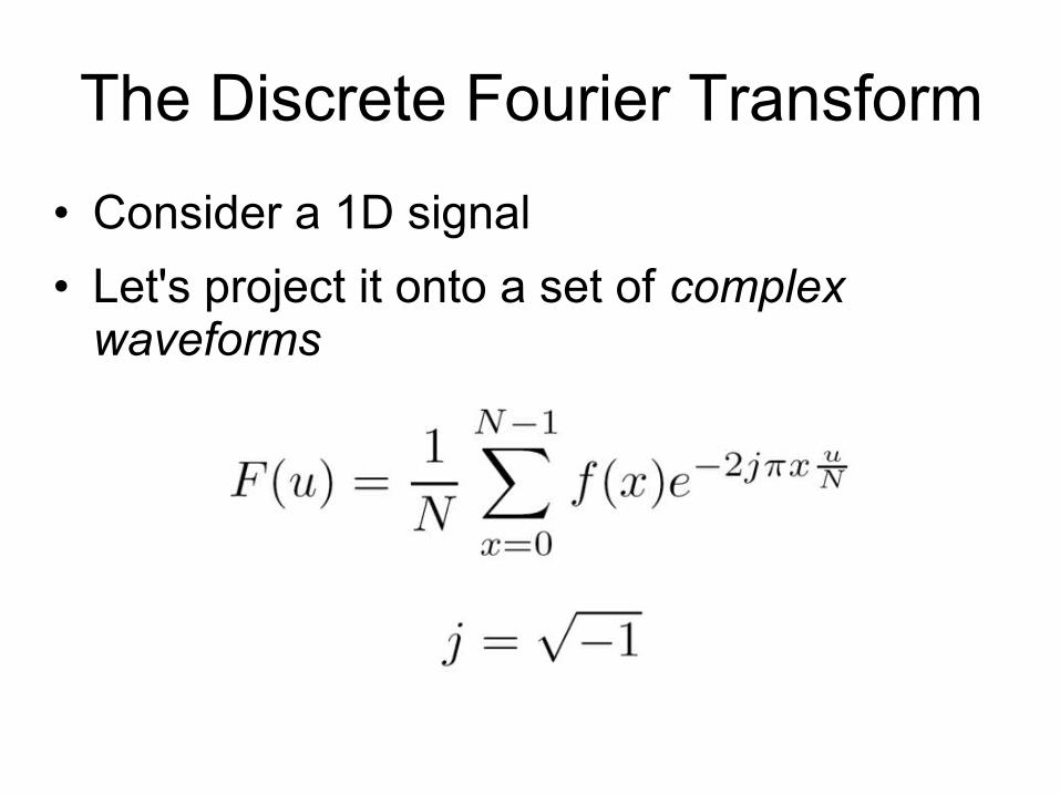
The Discrete Fourier Transform
• Consider a 1D signal
• Let's project it onto a set of complex waveforms
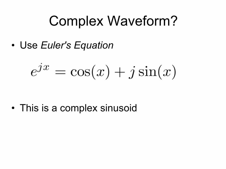
Complex Waveform?
• Use Euler's Equation
• This is a complex sinusoid
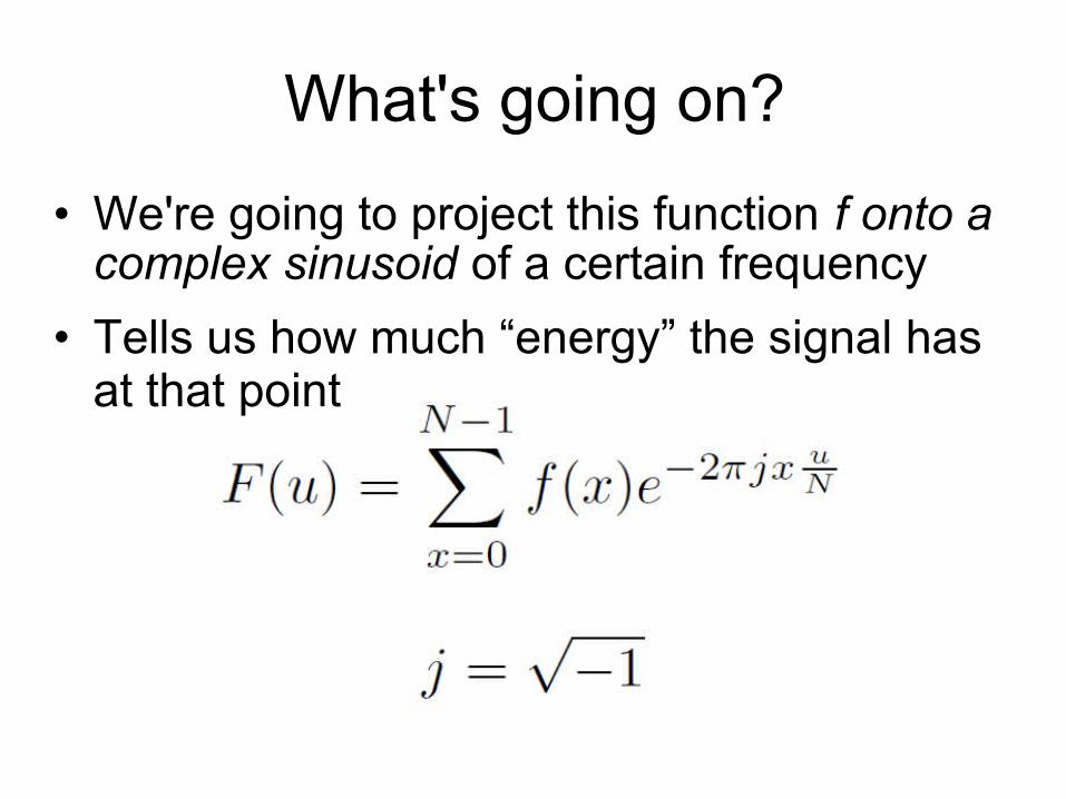
What's going on?
• We're going to project this function f onto a complex sinusoid of a certain frequency
• Tells us how much “energy” the signal has at that point
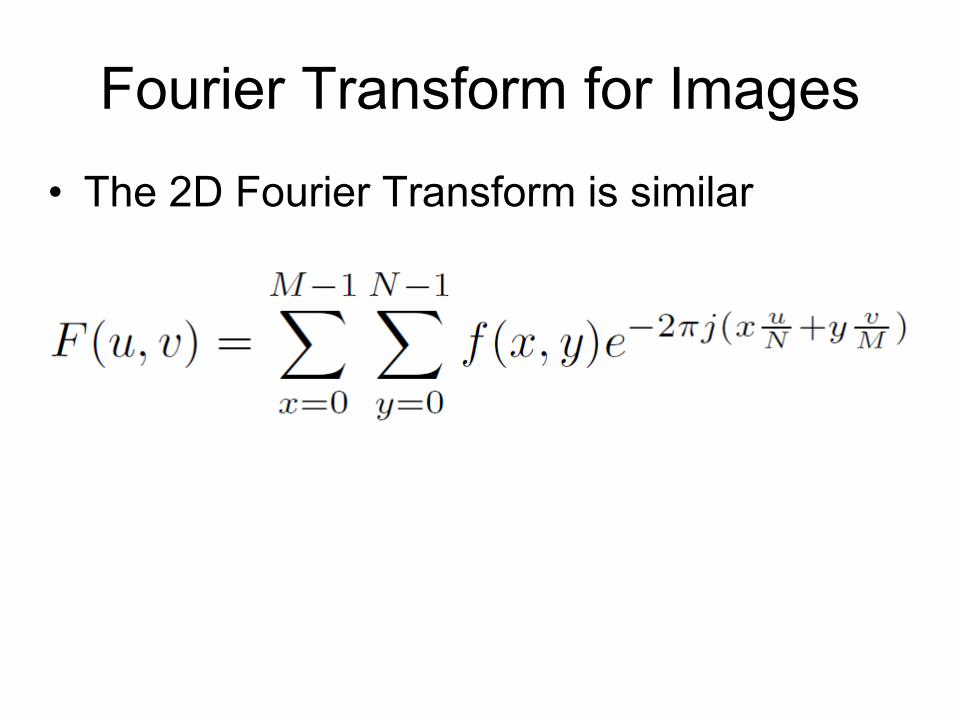
Fourier Transform for Images
• The 2D Fourier Transform is similar

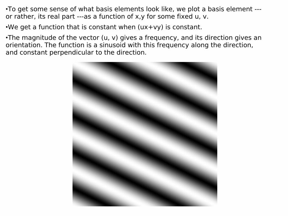
•To get some sense of what basis elements look like, we plot a basis element --- or rather, its real part ---as a function of x,y for some fixed u, v.
•We get a function that is constant when (ux+vy) is constant.
•The magnitude of the vector (u, v) gives a frequency, and its direction gives an orientation. The function is a sinusoid with this frequency along the direction, and constant perpendicular to the direction.

Here u and v are larger than in the previous slide.

And larger still...
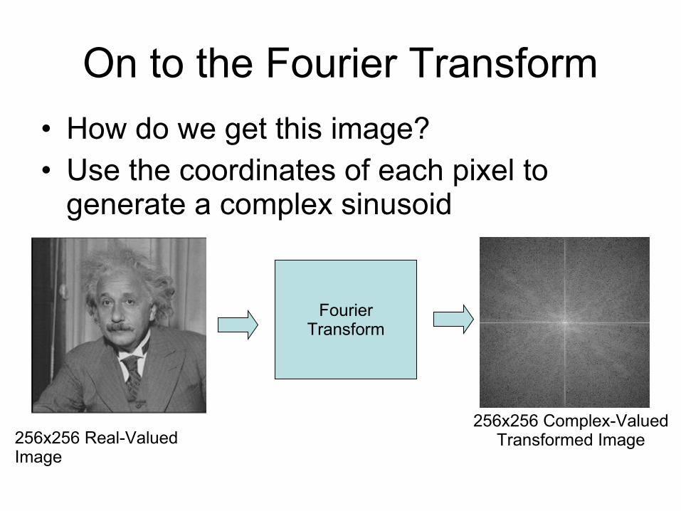
On to the Fourier Transform
• How do we get this image? • Use the coordinates of each pixel to
generate a complex sinusoid
Fourier Transform
256x256 Complex-Valued Transformed Image256x256 Real-Valued
Image
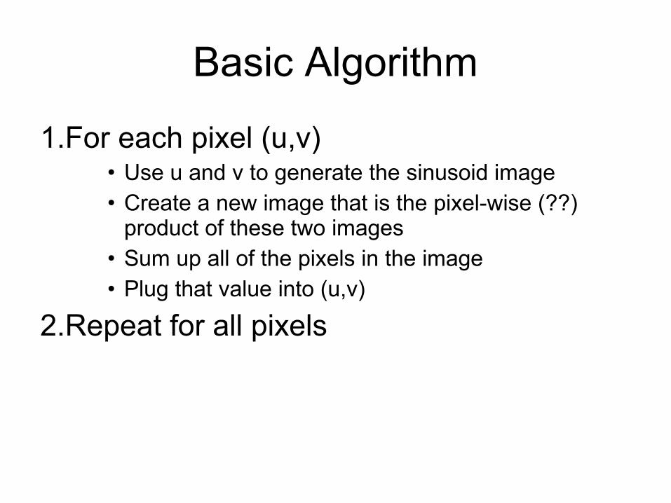
Basic Algorithm
1.For each pixel (u,v)• Use u and v to generate the sinusoid image• Create a new image that is the pixel-wise (??)
product of these two images• Sum up all of the pixels in the image• Plug that value into (u,v)
2.Repeat for all pixels
•To get some sense of what basis elements look like, we plot a basis element --- or rather, its real part ---as a function of x,y for some fixed u, v.
•We get a function that is constant when (ux+vy) is constant.
•The magnitude of the vector (u, v) gives a frequency, and its direction gives an orientation. The function is a sinusoid with this frequency along the direction, and constant perpendicular to the direction.

Here u and v are larger than in the previous slide.

And larger still...
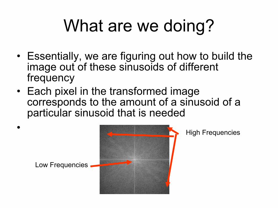
What are we doing?
• Essentially, we are figuring out how to build the image out of these sinusoids of different frequency
• Each pixel in the transformed image corresponds to the amount of a sinusoid of a particular sinusoid that is needed
•
Low Frequencies
High Frequencies
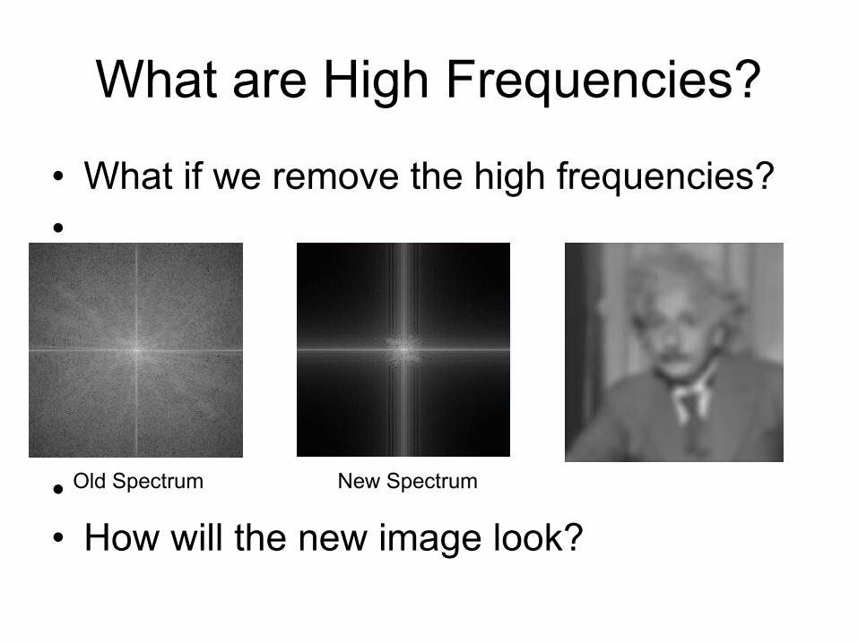
What are High Frequencies?
• What if we remove the high frequencies?••••••• How will the new image look?
Old Spectrum New Spectrum
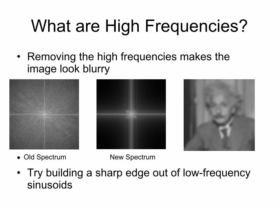
What are High Frequencies?
• Removing the high frequencies makes the image look blurry
••••••• Try building a sharp edge out of low-frequency
sinusoids
Old Spectrum New Spectrum
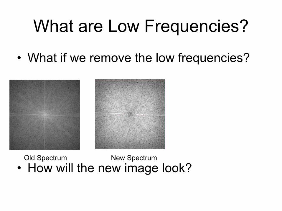
What are Low Frequencies?
• What if we remove the low frequencies?
• How will the new image look?Old Spectrum New Spectrum

What are Low Frequencies?
• What if we remove the low frequencies?
• How will the new image look?Old Spectrum New Spectrum
Working with the DFT (Discrete Fourier Transform)
• Is the complex part bothering you yet?
• Let's look at a different representation
• Every complex number can also be represented as
• z = x + jy = rejθ
• r – magnitude (real number)
• θ - Phase
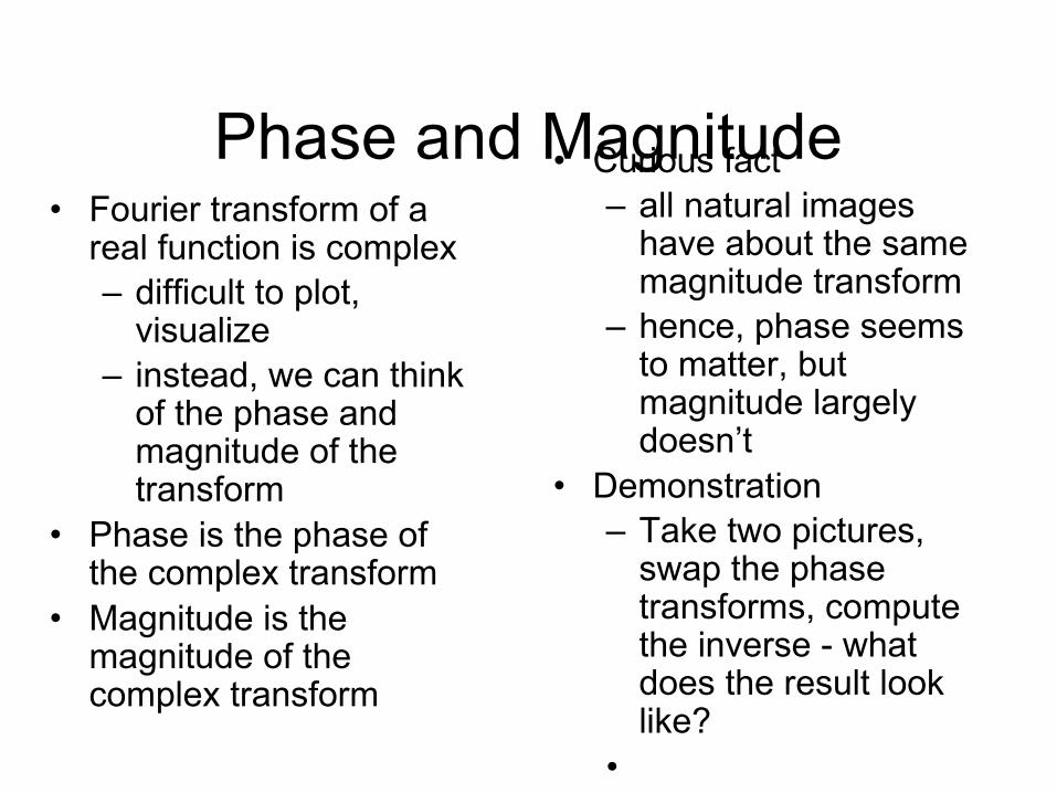
Phase and Magnitude• Fourier transform of a
real function is complex– difficult to plot,
visualize– instead, we can think
of the phase and magnitude of the transform
• Phase is the phase of the complex transform
• Magnitude is the magnitude of the complex transform
• Curious fact– all natural images
have about the same magnitude transform
– hence, phase seems to matter, but magnitude largely doesn’t
• Demonstration– Take two pictures,
swap the phase transforms, compute the inverse - what does the result look like?
•
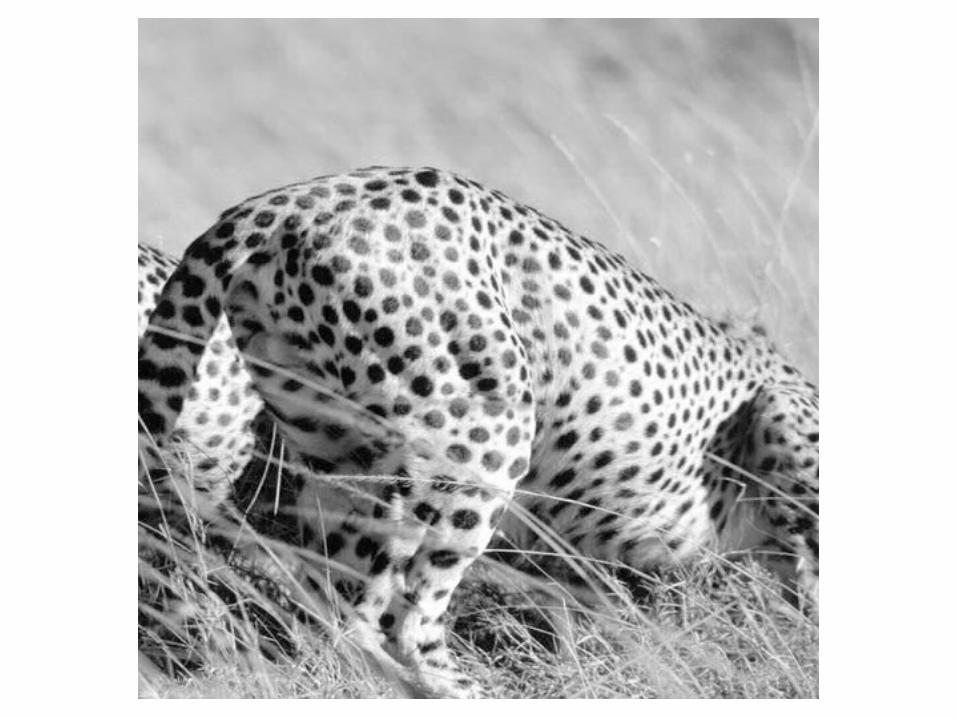
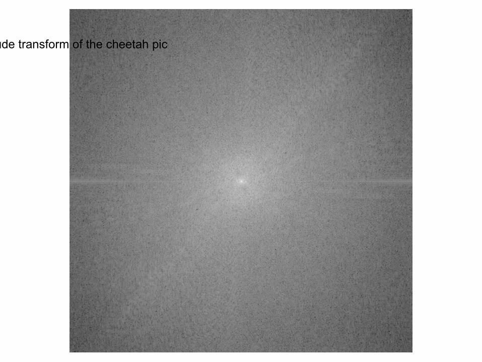
This is the magnitude transform of the cheetah pic
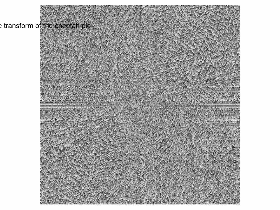
This is the phase transform of the cheetah pic
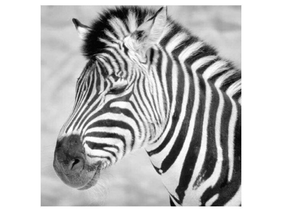
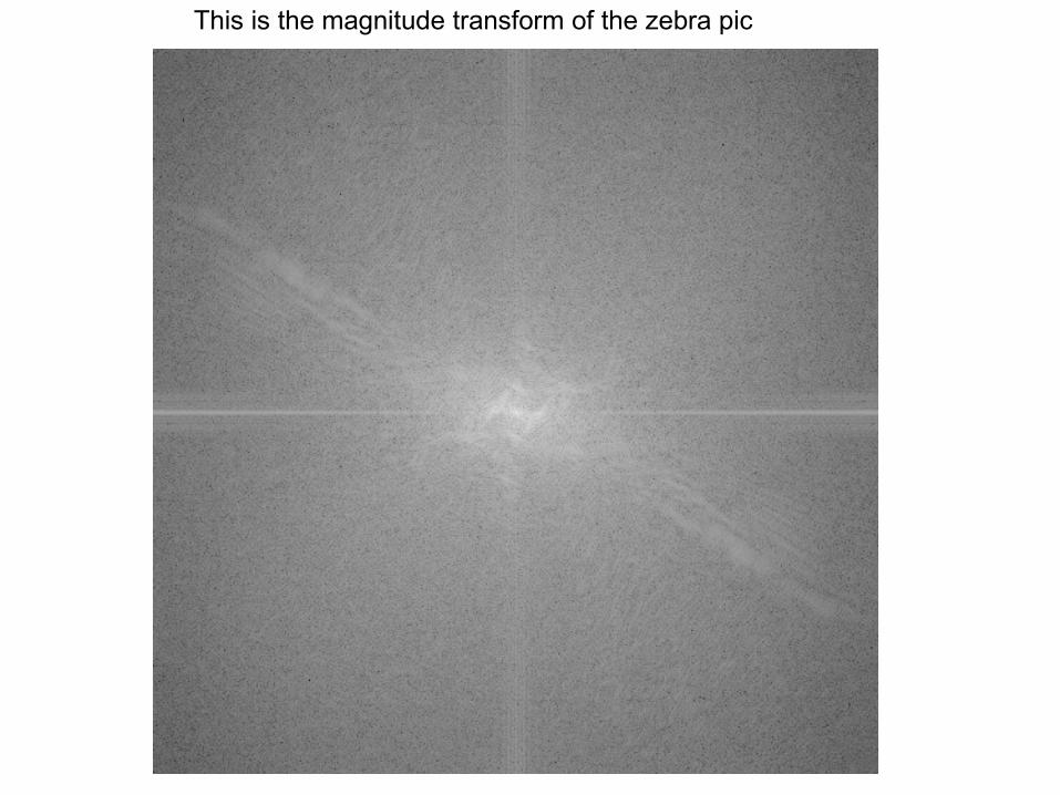
This is the magnitude transform of the zebra pic
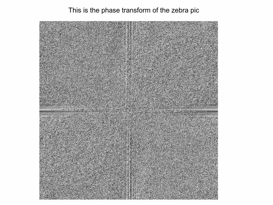
This is the phase transform of the zebra pic
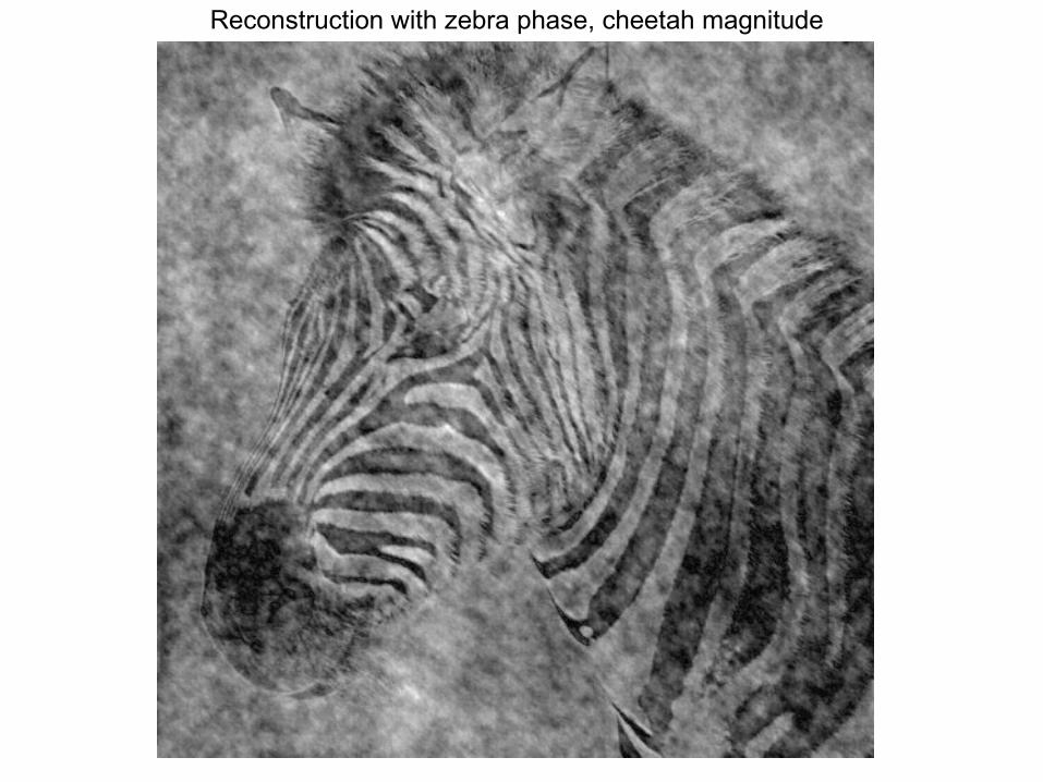
Reconstruction with zebra phase, cheetah magnitude
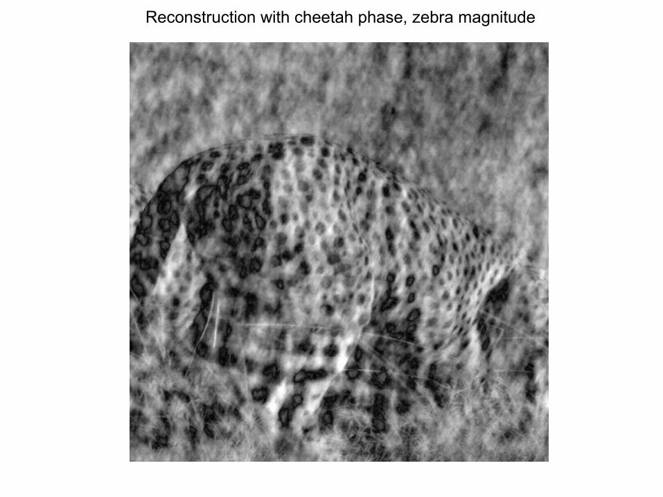
Reconstruction with cheetah phase, zebra magnitude

The Fourier Transform Helps Us Analyze Convolutions
•Notation: f(x,y) is the signal, F(u,v) is the DFT•If h = f * g ← Convolution–Then H(u,v) = F(u,v)G(u,v)–Convolution in the spatial domain is multiplication in the Fourier domain–You'll derive this in the problem set
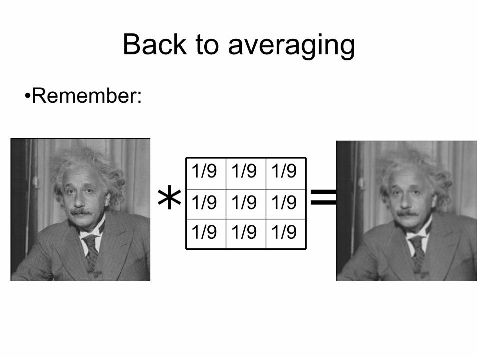
Back to averaging
•Remember:
*1/91/91/9
1/91/91/9
1/91/91/9
=
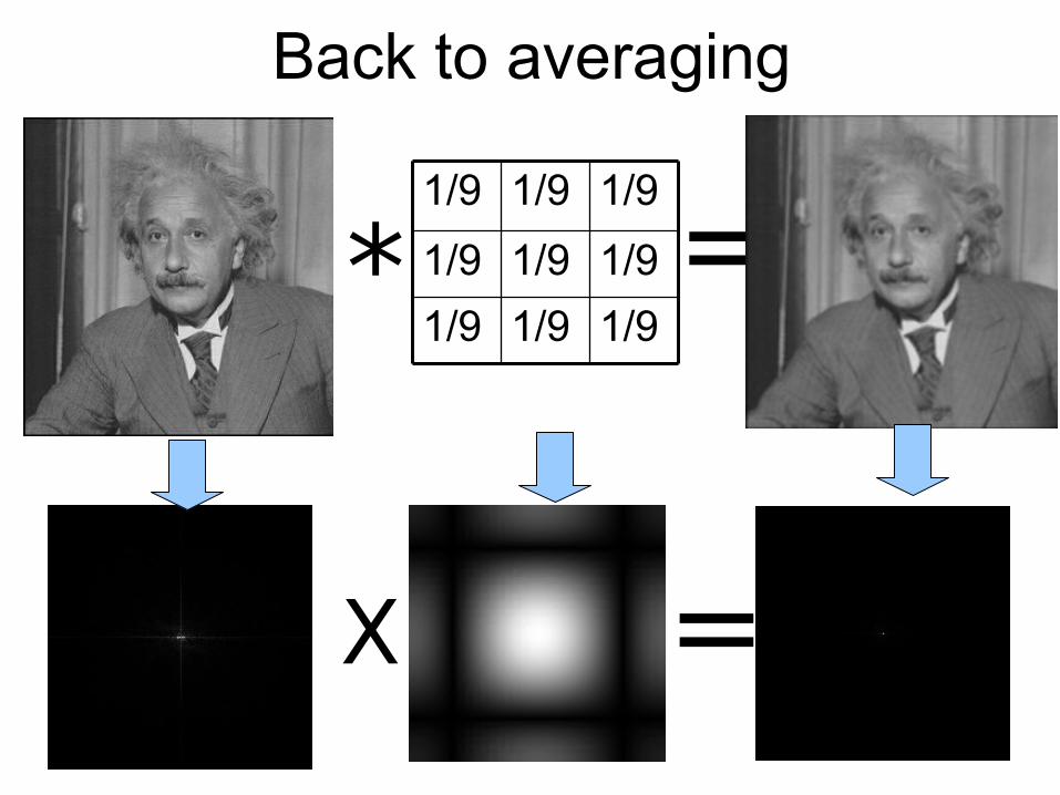
Back to averaging
*1/91/91/9
1/91/91/9
1/91/91/9
=
X =
Filtering
• We pixel-wise multiply the DFT of the input image by the DFT of the filter
• Frequencies where the magnitude of the response of the filter are near zero (black in the images) will be eliminated
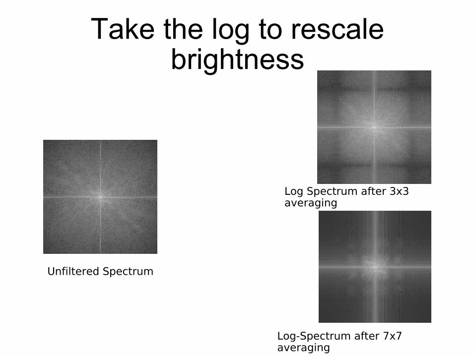
Take the log to rescale brightness
Unfiltered Spectrum
Log Spectrum after 3x3 averaging
Log-Spectrum after 7x7 averaging

Back to this example
•With σ set to 1 With σ set to 3
Input
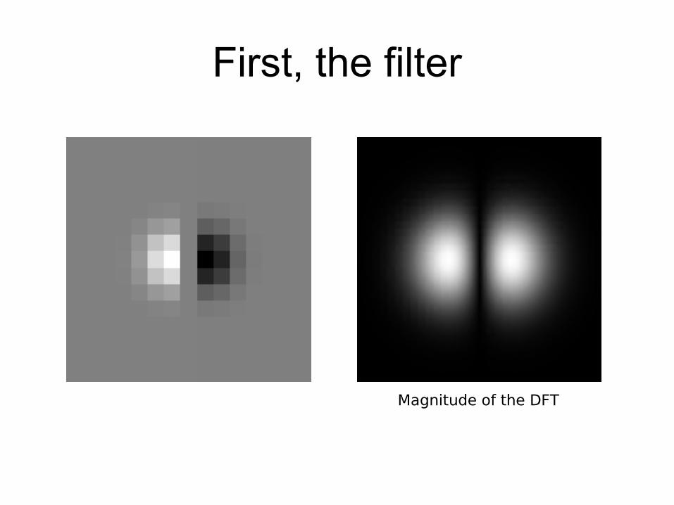
First, the filter
Magnitude of the DFT
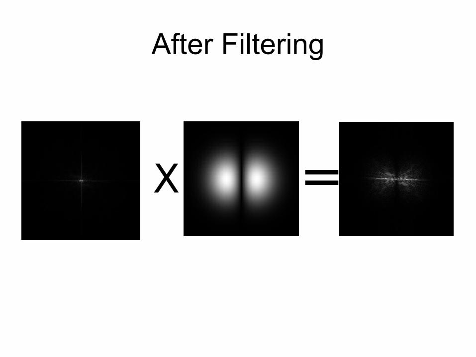
After Filtering
X =

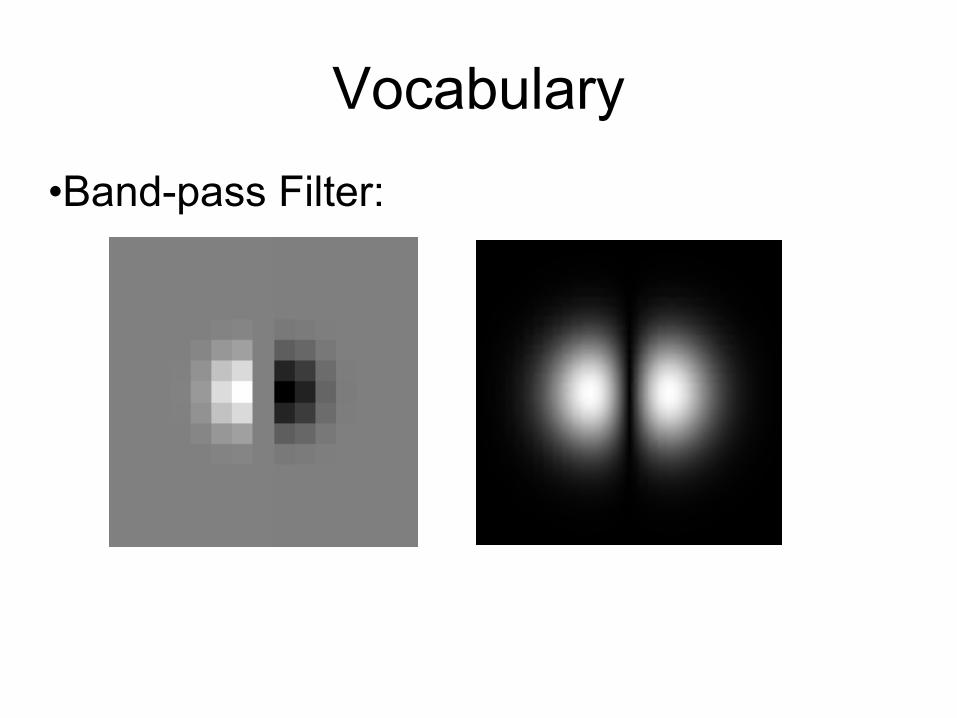
Vocabulary
•Low Pass Filter:
1/91/91/9
1/91/91/9
1/91/91/9
Vocabulary
•Band-pass Filter:
Vocabulary
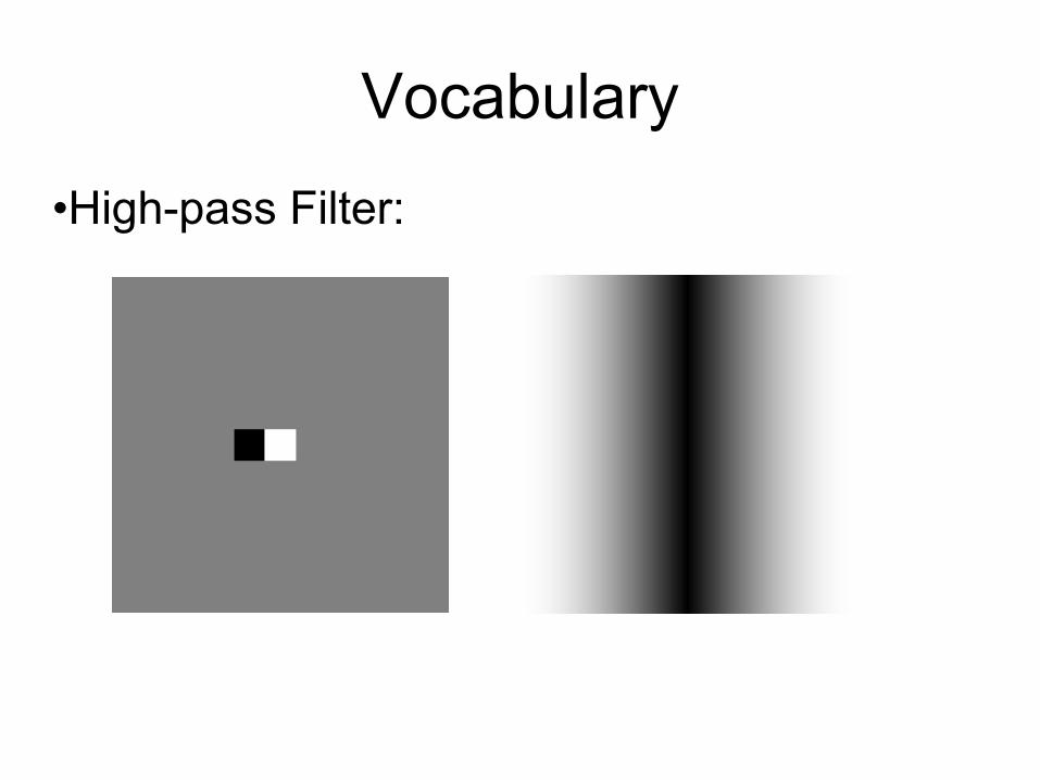
•High-pass Filter:
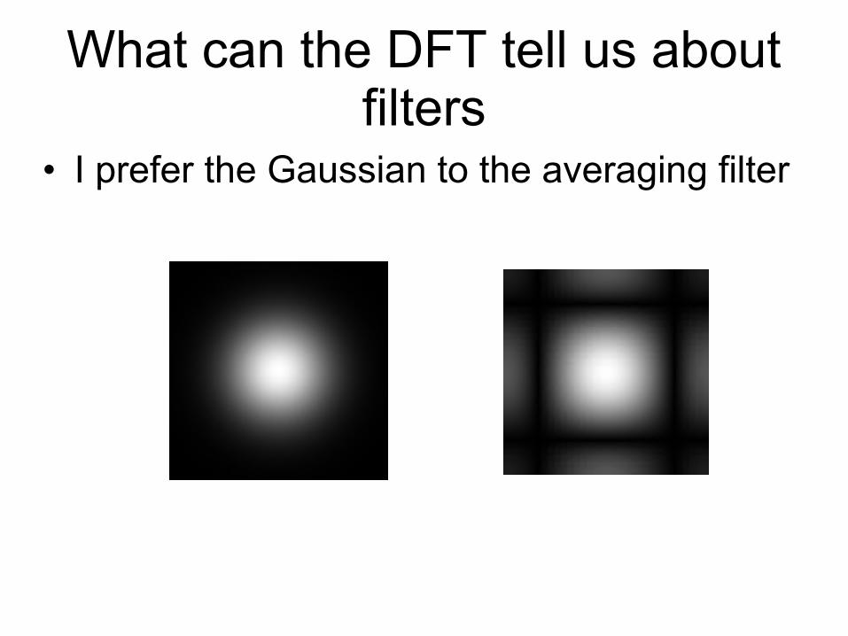
What can the DFT tell us about filters
• I prefer the Gaussian to the averaging filter
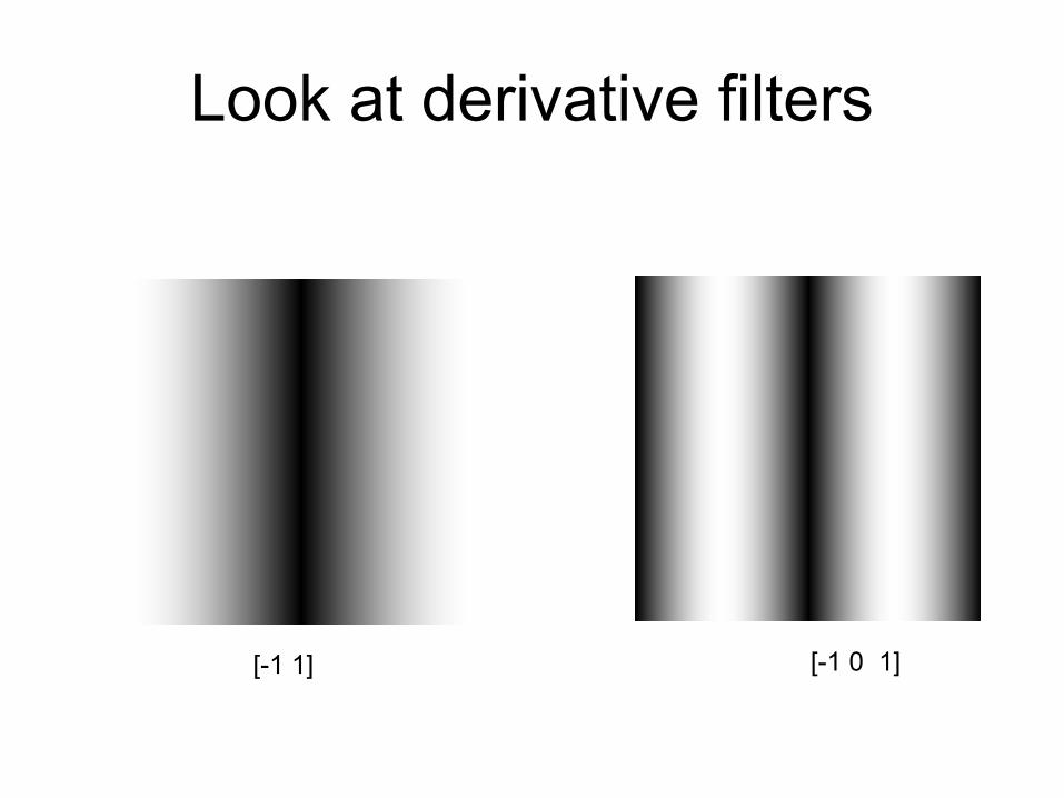
Look at derivative filters
[-1 1] [-1 0 1]