1

Capital Accumulation, Private Property

and Rising Inequality in China, 1978-2015

Appendix

Thomas Piketty (Paris School of Economics)

Li Yang (World Bank and Paris School of Economics)

Gabriel Zucman (UC Berkeley and NBER)

October 7, 2018

This appendix supplements our paper and describes the full set of data files and

computer codes (PYZ2017.zip) that were used to construct the series.

2

Appendix A. National income and wealth accounts series

Appendix B. Income and wealth distribution series

References

The zip file PYZ2017.zip includes the following files (in addition to the pdf files of the

main paper and present appendix):

PYZ2017MainFiguresTables.xlsx : figures and tables presented in the main paper

PYZ2017NationalAccountsData.zip : all national accounts files

PYZ2017DistributionSeries.zip : all distribution series files

PYZ2017IncomeDistributionData.zip : all raw income distribution files

PYZ2017WealthDistributionData.zip : all raw wealth distribution files

Note: the file PYZ2017.zip is relatively large (about 1.5Go), so we also provide on-line

access to PYZ2017MainFiles.zip, which solely includes the main data files.

3

Appendix A. National income and wealth accounts series

A1: National Balance Sheet

A11: Housing

A12: Agriculture Land

A13: Household Non-Equity Financial Assets and Liability

A14: Corporate Assets and Liabilities

A15: Government Assets and Liabilities

A16: Foreign Assets and Liabilities

A17: Private Share vs. Public Share

A2: National Income Series

A21: Real Growth and National Income

A22: Capital Depreciation (KDt)

A23: Flow of Funds

A24: Public Revenue

4

Appendix A. National income and wealth accounts series

Our detailed national income and national wealth series are presented in the file

PYZ2017NationalAccountsData.xlsx. This file includes a large number of tables

presenting different breakdowns and decomposition of national income and national

wealth by income and asset categories, following SNA 2008 concepts and the

distributional national accounts guidelines of Alvaredo et al (2016). A general

discussion about data sources, methodological and conceptual issues regarding

national accounts is provided in the paper (section 2.1). The file includes more detailed

explanations on how our series were constructed.

We also provide access to a directory including the raw material from official and non-

official series that were used to construct these series

(PYZ2017NationalAccountsData).

The zip file PYZ2017NationalAccountsData.zip contains both the .xlsx file with the

detailed series and the raw material directory and is included in the zip file

PYZ2017.zip.

A1: National Balance Sheet

The National Bureau of Statistics (NBS) published a guide book for compiling China’s

national balance sheet1 in 1997 and has compiled national balance sheets on a trial

basis since then. However, these balance sheets have never been published (Faqi Shi

2011). Over the last decade, a number of studies have attempted to construct the

1 Methods for Compiling the Balance Sheet of China, 1997. An updated version of the book was published in 2007.

5

balance sheet of China. The most important studies are those of Ma et al. (2012), Cao

et al. (2012) and especially Li et al. (2013a, 2013b 2015). Li and his research team

from the Academy of Social Sciences of China estimate China’s balance sheet from

2007 to 2014. For some sectors – including households – the data cover the 2000 to

2014 period. They cover both public and private sectors. This is one the most complete

attempts to estimate China’s national wealth so far.

Following the U.N. System of National Accounts 2008 (SNA 2008), the NBS National

Account Guide Book (National Balance Sheet Guide Book 2007, GDP Guide Book

2007), together with previous studies (Ma, 2012, Li, 2013a, 2013b, 2015), we

constructed the national balance sheet of China for the period of 1978-2015.

Comparing to previous studies, there are several innovations in our research.

1. We extend the national balance sheet for longer period, i.e. Li, Y et. al. (2013a)

covers the period of 2007-2011, Ma, J et. al (2012) covers the period of 2002-2010,

we estimate the national balance sheet for the period 1978-2015.

2. We study flows together with stocks, i.e. by combining China’s official flow of

funds table and national balance sheet. This enable us to estimate 1) capital returns

by different assets in each institutional sector and 2) saving effect and pricing effect of

wealth accumulation by different assets in each institutional sector.

3. We estimate private and public share by assets, i.e. housing, farmlands,

corporate equity.

4. We estimate both book value and market value national wealth.

5. Last but not the least, we are 100% transparent with our estimation, assumption

as well as data source. All the data used for estimation is included in appendix

6

“PYZ2017NaitonalAccountsData”, while Li, Y. et. al. (2013a) and Ma, J. et. al (2012)

only provide explanation of their estimating method and the final estimation results of

the national balance sheets.

In what follows, we describe our estimation method in detail.

A11: Housing

We estimate the market value of urban housing and of rural housing separately. More

specifically, for each year t between 1978 and 2015 we define:

𝑈𝐻𝑡𝑚𝑣: market value of urban housing in year t

𝑁𝑈𝐻𝑡𝑚𝑣: market value of new urban housing in year t

𝑈𝐶𝐺𝑡: urban housing capital gain during year t

𝑈𝐾𝐷𝑡: urban housing depreciation during year t

𝑈𝑃𝑂𝑃𝑡: urban population in year t2

𝑈𝐿𝑆𝑝𝑐𝑡: urban per capita living space (square meters) in year t

𝑈𝑃𝑡: average residential house selling price (RMB per square meter) in year t

We have the following accounting relationships:

𝑈𝐻𝑡𝑚𝑣 = 𝑈𝐻𝑡−1

𝑚𝑣 + 𝑈𝑁𝐻𝑡𝑚𝑣 + 𝑈𝐶𝐺𝑡 − 𝑈𝐾𝐷𝑡

𝑈𝑁𝐻𝑡𝑚𝑣 = (𝑈𝑃𝑂𝑃𝑡 ∗ 𝑈𝐿𝑆𝑝𝑐𝑡 − 𝑈𝑃𝑂𝑃𝑡−1 ∗ 𝑈𝐿𝑆𝑝𝑐𝑡−1) ∗ 𝑈𝑃𝑡

2 In our paper, we use the concept of permanent residence from NBS National Census to define, “urban population”, namely residents with urban Hukou and rural migrants who had lived in cities for more than six months.

7

𝑈𝐶𝐺𝑡 − 𝑈𝐾𝐷𝑡 = 𝑈𝑃𝑂𝑃𝑡−1 ∗ 𝑈𝐿𝑆𝑝𝑐𝑡−1 ∗ (𝑈𝑃𝑡 − 𝑈𝑃𝑡−1)

𝑈𝐾𝐷𝑡 = 𝑈𝐻𝑡−1𝑚𝑣 ∗ 𝑈𝑟𝑏𝑎𝑛 ℎ𝑜𝑢𝑠𝑖𝑛𝑔 𝑑𝑒𝑝𝑟𝑒𝑐𝑖𝑎𝑡𝑖𝑜𝑛 𝑟𝑎𝑡𝑒

Due to the lack of detailed data on urban housing construction before 1978, we are not

able to calculate the housing value before 1978 directly. To estimate the urban housing

value in 1978, we make the following assumptions:3

1) The average housing age in 1978 is 15 years, meaning the average urban

house was built in 1963,

2) The total urban housing living area is equal to 𝑈𝑃𝑂𝑃1978 ∗ 𝑈𝐿𝑆𝑝𝑐1978.

3) The urban housing depreciation rate is 2% (NBS GDP Guide Book, 2007).

4) The average residential house selling price was constant during 1963 to 1978

and equal to 𝑈𝑃1978. Since this price is the selling price of newly built houses,

depreciation needs to be considered when calculating the selling price of old

houses. For example, in 1978, the selling price of houses which were built in

1963 is set equal to 𝑈𝑃1963 ∗ (1 − 0.02)15. This assumption reflects the fact that

old houses were much cheaper than new houses, because of the lack of

investment in home improvement to offset depreciation.

Based on these assumptions, we have,

𝑈𝐻1978𝑚𝑣 = 𝑈𝑃𝑂𝑃1978 ∗ 𝑈𝐿𝑆𝑝𝑐1978 ∗ 𝑈𝑃1978 ∗ (1 − 0.02)15

The market value of rural houses is estimated in the same way, except the rural

housing depreciation rate is set equal to 3% (based on NBS GDP Guide Book, 2007).

Our method is similar to the one used in Li (2013a).

3 Since in 1978 the stock value of urban housing is small, post 1990s house values are not affected much by these assumptions.

8

A12: Agriculture Land

Evolution of Agriculture Land Policy in China

After the 1949 Communist Revolution, eliminating the private economy was a national

policy for over 30 years. In rural China, all the means of production (land, machines,

etc.) were transferred to the People’s Commune, peasants were organized into

production team working on the land to meet State quotas. Due to the lack of incentives,

agricultural output stagnated. Launched in the early 1980s after more than two

decades of collective farming, the household responsibility system (HRS) aimed at

providing solution to this long-lasting problem.

The HRS was an agriculture production system which allowed households to contract

land, machinery and other facilities from collective organizations. The aim was to

preserve a basic unified management of the collective economy while contracting out

land and other goods to households.4 Households could make operating decisions

independently within the limits set by the contract agreement, and could freely dispose

of surplus production over and above national and collective quotas. HRS was created

by the peasants but spread nationally with the support of the central government. By

1983 more than 93 percent of production teams had adopted the system.

The HRS enables farmers to contract land from collective organizations. In 1984, CPC

Central Committee document no. 1 5 stipulated that contracts for farmland should

generally last more than 15 years. The 1984 document also stipulated that privately-

farmed plots of cropland and contract cropland were not allowed to be sold, rented out,

or transferred into homestead or other non-agricultural land. In 1986, HRS was written

4 “Summary of National Rural Work Conference” (CC [1982], No.1) defined the socialism nature of Household Responsibility System. 5 “Notice Regarding 1984 Rural Work” (CC [1984], No.1)

9

into the first “Land Administration Law of the PRC” and added into the Constitution of

the PRC in 1993. In 1997, the policy document regarding the second round of land

contracts emphasized that contracts should be extended to 30 years. 6 In 2009,

policymakers re-emphasized that contract relationships would remain unchanged for

a very long time.7

The transfer of the use of the land has been gradually legalized over the last 30 years.

In 1982, the Constitution of the PRC stipulated that “Land in the rural and suburban

areas is owned by collectives except for those portions which belong to the state in

accordance with the law; homestead and privately farmed plots of cropland and hilly

land are also owned by collectives. The state may in the public interest take over land

for its use in accordance with the law. No organization or individual may appropriate,

buy, sell or lease land, or unlawfully transfer land in other ways (emphasis added)”

(Article 10). This changed with the adoption of the 1988 Constitution Amendment. The

fourth paragraph of Article 10 was amended as follows: “No organization or individual

may appropriate, buy, sell or unlawfully transfer land in other ways. The right to the

use of the land may be transferred in accordance with the law” (emphasis added).

The 1988 Land Use Regulation Law Amended states: “The right to the use of the state

land may be transferred in accordance with regulations provided by the State Council.

The state land may be used with just compensation, which is regulated by the State

Council.” This provision can be interpreted as legalizing the transfer of land use rights

with restrictions.

6 “Notice Concerning Further Stabilizing and Perfecting the Rural Land Contracting Relationship, the Cent. Comm. of the Chinese Communist Party and the State Council” (GOCC [1997], No. 16) 7 “Certain Opinions of the State Council and the Cent. Comm. of the Chinese Communist Party on Promoting the Stable Development of Agriculture and Continuing to Increase Farmers’ Income in 2009” (CC [2009], No.1)

10

In 2002, the Rural Land Contracting Law was enacted. It allows limited land-use

transfers between individual farmers. However, it does not permit unrestricted trade

between farmers and companies and straight sales of land-use rights or the option to

use the land as collateral to obtain a loan. In 2009, State Council and the Central

Committee of the Chinese Communist Party issued a policy aimed at “establishing and

perfecting markets for transferring contractual land management rights”. 8 In

September 2016, the Ministry of Agriculture issued “the Rules for the Operation of the

Circulation and Trading Markets of the Right to Manage Rural Land (for Trial

Implementation)”, which provides the guideline for market-oriented agricultural land

transaction.

Estimation of Market Value of Crop Land

Due to the nature of collective ownership of rural land in China and the

underdevelopment of agricultural land market, one cannot observe rents and market

price of agriculture land directly. In order to estimate the market value of agricultural

land, indirect method must be used. We proceed as follows.9

The World Bank (2005) and the UN (2012) estimate China’s land values based on the

present discounted value of land rents. Land rents are estimated as a percentage of

production revenue from an array of crops sold on world market10. Total land rent is

the area-weighted average of rents from major crops. Although they use similar

methods, the World Bank (2005) and the UN (2012) estimations of the market value of

China’s crop land are quite different from each other. The World Bank (2005) estimates

8 “Certain Opinions of the State Council and the Cent. Comm. of the Chinese Communist Party on Promoting 9 We only include cropland but not forest or pasture when estimating the market value of agricultural land. 10 9 crops are selected as the representative crops in World Bank (2005), while 159 crops are selected as the representative crops.

11

that the market value of China’s cropland in 2000 was 24,235 billion RMB (in 2015

RMB). The UN estimate for the same year is 8,380 billion RMN (in 2015 RMB).

We do not take a stance on which estimate is correct. Estimating agricultural rents

under China’s rural land system is fraught with uncertainties. Instead, we adopt a much

simpler method to estimate the market value of cropland – the compensation method,

which is one of the proposed methods in the literature for the farm land value estimation.

We choose to use this method since 1) compensation and land expropriation is the

only farmland transaction that could be observed, 2) comparing to other methods,

compensation method requires less assumptions and calculations.

Based on Land Management Law (LML) of PRC (1998), there are three different type

of compensations for requisitioned arable land.

a. compensation for requisitioned arable land shall be six to ten times the average

annual output value of the requisitioned arable land, calculated on the basis of three

years preceding such requisition.11

b. Resettlement subsidies for requisitioned arable land shall be calculated

according to the agricultural population needing to be resettled. The agricultural

population needing to be resettled shall be calculated by dividing the area of

expropriated cultivated land by the average area of the original cultivated land per

person of the unit the land of which is expropriated. The standard resettlement

subsidies to be divided among members of the agricultural population needing

resettlement shall be four to six times the average annual output value of the

expropriated cultivated land calculated on the basis of three years preceding such

11 Based on LML of PRC (1986), the compensation rate is three to six.

12

expropriation. However, the maximum resettlement subsidies for each hectare of the

expropriated cultivated land shall not exceed fifteen times its average annual output

value calculated on the basis of three years preceding such expropriation.12

c. Rates of compensation for attachments and young crops on requisitioned arable

land shall be prescribed by provinces, autonomous regions and municipalities directly

under the Central Government.

In our research, the resettlement subsidies are not included as a part of the value of

the requisitioned arable land. In theory, the resettlement subsidies are the

compensation paid by the government to farmers for unexpected life changing, such

as losing farm lands. This compensation can be treated as a one-time social security

payment for “laying off” the farmers from lands. Also based on LML (1998), the

resettlement subsidies are paid by person, not by the area of the land.

We also exclude the compensation for attachments and young crops on expropriated

land from farm land value, since in our research we are only interested at the value of

the farm land, not the value of the young crops and attachments on the farm land.

We assume that the market value of cropland is equal to the potential compensation

of the land. To avoid discontinuity in the land value series, we adopt 6 times the

average output of the land in the last 3 years as the average compensation standard

for the whole period. Our estimate of the market value of cropland in 2000 is 14,635

billion RMB (2015 RMB), which is in between the estimate of the World Bank (2005)

and of the United Nations (2012).

12 The compensation standards for requisitioned arable land was first stipulated in “State Construction Land Acquisition Regulations (1982)”. Before 1998, the compensation rate is three to six (see LML of PRC (1986)), LML of PRC (1998) the compensation rate increased to six to ten, and has remained the same ever since.

13

As one robustness check, we compare the farmland value/output ratio across different

countries. As we can see in Table 1 below, the farmland value/ output ratio is between

4 to 12 for USA and 4 other European countries for the period of 2000-2005. This

signals that that our assumption (farmland value/farmland ratio=6) is in line with other

countries.

Table 1

Country Year

Farmland Value /Output

Ratio USA 2002 7.1

France 2005 3.7 Spain 2005 12.0

Poland 2005 4.3 Ireland 2000 9.5

Notes: Results are estimated by authors based on agricultural data from USDA (USA), Eurostat, and CSO (Ireland). As another robustness check, we estimate an alternative land value series using a

different assumption: the ratio of land value over farming value added is 10 (this is

equal to assume that capital income (rent) of land from farming accounts for 40% of

farming value added, discount rate is 4%). Then we compare our results with the

estimation from UN (2012) and World Bank (2005). Please see Table 2.

Table 2

Year Estimation (in 2015 billion RMB) Crop Land Value

Crop Land Value/Output

Crop Land Value/farming

value added

2000 UN (2012) 8,380 3.4 6.1 2000 World Bank (2005) 24,235 9.9 17.6 2000 Method I: crop land/output=6 14,635 6 10.6 2000 Method II: crop land/value added= 10 13,742 5.6 10

Notes: UN estimation of crop land value is from "UN Inclusive wealth report 2012". World Bank estimation of crop

land is from the World Bank 2005 "Where is the Wealth of Nations?: Measuring Capital for the 21st Century."

Estimations of Method I and II are from PYZ2017NationalAccountsData, AP10.

As we can see, the estimations of crop land value based on two methods are close to

each other. In UN (2012), the estimation the value of farmland in China almost did not

14

change during the period of 1990-2008 (it decreased around 5% in 2007 and 2008),

which contradicts the fact that the output of farm land (in 2015 yuan) in China has

increased 50% during the same period. Meanwhile, World Bank (2005) estimation

indicates that the ratio of land value over farming value added is around 18. This

implies that, if the discount rate is 4%, then the capital income (rent) of the crop land

is 72% of total farming value added, which we believe is too high for China’s reality.

A13: Household Non-Equity Financial Assets and Liability

Currency and bonds held by households are estimated based on the methods

described in the NBS national balance sheet guide book (1997, 2007). Currency held

by households is set equal to M0 times 80%. Bonds held by households are set equal

to the outstanding stock of national treasury bonds times 65%, plus outstanding

financial bonds13 times 2.5%, plus corporate bond. The fraction of national currency

and bonds held by the household sector is estimated by the NBS based on annual

Flow of Funds statistics.14

The value of the deposits and loans of households are set equal to the value of the

saving deposits of urban and rural household published by NBS.15

As in Li (2013a), data on household insurance and pension funds and liabilities are

taken from “China Financial Stability Report” (2012, p. 90) and “Sources and Uses of

Credit Funds of Financial Institutions” (People’s Bank of China), which only cover the

period after 2004. Using the Flow of Fund of China (1992-2014), we extend the data

for the period 1992 to 2004, assuming that changes in wealth are only caused by

13 Bonds issued by financial institutions, such as central bank, policy banks, and commercial banks. 14 See, “NBS national balance sheet guide book (1997)”, P18 15 From 2011 to 2014, data is from "Credit balance table of financial institutions, source”; before 2011, data is from "urban and rural household savings".

15

saving flows and not valuation (i.e., the capital gains of household insurance and

pension funds are set equal to 0 during the period). Before 1983, we assume the value

of household insurance and pension funds is 0. 16 For the years between 1992 and

1983, we use linear interpolations.

A14: Corporate Assets and Liabilities

Balance Sheet of Corporate Sector (1992-2015)

There are two steps to estimate the balance sheet of corporate sector.

First, we estimate the book value of the total assets and liabilities of the corporate

sector. To do so, we estimate assets and liabilities by industry,17 using available data

from different sources,18 and then add up the figure to the national level.

Second, we split the book value total assets into non-financial assets and financial

assets. There are two ways to do this.

Method 1: we first calculate the ratio of financial assets to total assets for listed

companies by industry and year using the China Stock Market & Accounting Research

(CSMAR) database19. We assume that the ratio is the same for unlisted companies as

16 In 1958, China close all the insurance business, only in 1982, life insurance business was re-introduced in China. 17 Including Agriculture, Industry (Mining, Manufacturing, Electric, Gas and Water Production and Supply), Construction, TSP (Transport, storage, and post), Wholesale and retail trade, Hotel and Catering, Real Estates, Financial Sector, and Others (Based on Industrial classification for national economic activities (GB/T 4754-2011)). 18 For example, China Basic Unit Census (1996, 2001), China Economic Census (2004, 2008, 2013), China Industrial Economy Statistical (2014) Yearbook and China Statistical Yearbook on Construction (2014), Almanac of China's Finance and Banking, NBS annual data base, etc. In most of the data sources, only total assets and liabilities of the industry are reported. Since data after 2013 is not available, we assume the real growth rate of total asset and liability of corporate sector in 2014 and 2015 is 0. 19 For financial sector, instead of using the balance sheet of listed companies from CSMAR, we are using the balance sheet of the big four commercial banks in China (the Bank of China, the China Construction Bank, the Industrial and Commercial Bank of China, and the Agricultural Bank of China).

16

for listed companies in the same industry and year. The book value of non-financial

asset is equal to total asset minus financial assets.

Method 2: We use the following identity:

Net household financial assets + Net government financial assets + Net foreign assets + Net corporate financial assets – Equity liability of corporate sector =0

The results of these two methods are close to each other: for most years, the difference

is less than 10%. 20 In order to comply with SNA (2008) guidelines and have a

consistent national balance sheet, we retain the second method. One drawback of the

first method is that it might not be realistic to assume that the financial ratio for listed

companies is the same as for unlisted companies, since listed companies in China are

generally much bigger than unlisted companies.

Book Value and Market Value of Equity in Corporate Sector (1978-2015)

For the period 1992-2015, we obtain the book value of corporate equity from the

corporate sector balance sheet constructed above.

For the period before 1992, we only have data on the equity of the industrial sector.21

To estimate total corporate equity, we have to make assumptions on the ratio between

the equity of the industry sector and the equity of the whole corporate sector (I/C ratio).

From 1986 to 1991, we are using the average I/C ratio for the period of 1992-1996,

20 The estimation results are in PYZ2016NationalAccountData, sheet AP1, column GN and GO. 21 Mining, Manufacturing, Electric, Gas and Water Production and Supply.

17

which is equal to 0.5. For the period of 1978 to 1985, we take the I/C ratio of Chow

(1993), namely 0.56.

There are two main stock exchanges in mainland China: the Shanghai Stock Exchange

and the Shenzhen Stock Exchange. The Shanghai Stock Exchange can be traced

back to 1891 when the Shanghai Share brokers’ Association was founded by foreign

businessmen in Shanghai. In 1904, the Association applied for registration in Hong

Kong and was renamed as the Shanghai Stock Exchange. After the creation of the

People's Republic of China in 1949, the stock exchange was closed. It was only re-

established in the end of 1990 after a 41-year hiatus. The Shenzhen Stock Exchange

was established in the same year as Shanghai Stock Exchange.

In order to calculate the market value of the corporate sector, we divide the corporate

sector into two groups, listed companies and unlisted companies. For listed companies,

the market value is equal to the total market capitalization (in China mainland). For

unlisted companies, we assume that the market value of equity is equal to the book

value of equity. The data series on total market capitalization start in 1992. Before 1992,

we assume that the market value of equities is equal to the book value of equities for

the whole corporate sector.

A15: Government Assets and Liabilities

In December 2014, the Ministry of Finance asked all levels of government to make

their balance sheets public by 2020. So far, however, there is no official government

balance sheet in China. Since 2010, there have been many attempts at constructing

government balance sheets (i.e. Tang, 2013, Li, 2013, 2015, Ma, 2012, Du, 2013).

Following previous studies, we estimate the government balance sheet following SNA

(2008) concepts and the NBS National Balance Sheet Guide Book (1997, 2007).

18

Accounting Entity

Due to the mixed nature of the Chinese economy, there has been a debate on the

definition of government assets and liabilities. In our study, we include into government

assets and liabilities the assets and liabilities of the general government, of public

financial institutions, and of State-invested enterprises.

The general government includes central and local administration (ADM), public non-

financial institution (PI), public institution managed as enterprises (PIE), and Social

Security Funds (SSF).

Public financial institution includes the People’s Bank of China, three Chinese policy

banks,22 four State-owned assets management companies23, and China Investment

Corporation.

State-invested enterprises are wholly state-owned enterprises, or companies in which

the State has a stake, whether controlling (the State share is greater than 50%) or non-

controlling (the State share is less than 50%). Following the NBS National Balance

Sheet Guide Book (1997, 2007), we include State-owned equities (also called national

capital) of State-invested enterprise in government financial assets.

Based on current financial accounting standards, 24 natural resources and public

housing under the management of the housing management department (HMD) are

not included in the assets of either ADM, PI, or PIE, which results in underestimating

government assets. We made a correction by adding public housing and natural

22 the Agricultural Development Bank of China (ADBC), China Development Bank (CDB), and the Export-Import Bank of China (Chexim) 23 China Great Wall Asset Management for the Agricultural Bank of China; China Orient Asset Management for the Bank of China; China Huarong Asset Management for the Industrial and Commercial Bank of China; China Cinda Asset Management for the China Construction Bank 24 Accounting system for administrative units, 1998 , Financial rules for administrative units, 2012, Accounting standards for public institutions, 1997, 2012.

19

resources to the government balance sheet. 25 Natural resources include publicly-

owned agricultural land and reserve land.

Government Assets

Government non-financial and financial assets are defined as follows:

Non-financial assets of ADM, PI, and PIE + Non-financial assets of public financial institution + Public housing + Natural resource = Non-financial assets Financial assets of ADM, PI, and PIE + Financial assets of public financial institution + SSF + Government fiscal deposit + Equity of State-invested = Financial assets

Li (2013b) defines government assets as resources that are either in the government’s

possession or under its control, and classifies them into 6 categories: business assets,

nonbusiness assets, natural resource assets, foreign assets, the social security fund,

and government deposits at the central bank.

Compared to Li (2013a, 2013b, 2015), there are several differences in our estimation

of government assets.

a. Li (2013a, 2013b, 2015) attributes all housing to the private sector. In our study,

we split housing into two part, private housing and public housing. Public

housing is included in government assets.

25 Natural resources are included in the assets of public sector based on SNA (2008), however it is not included by NBS National Balance Sheet Guide Book (1997, 2007). Public housing is included as government assets in by NBS National Balance Sheet Guide Book (1997, 2007).

20

b. Li (2013a, 2013b, 2015) includes all agricultural land into government assets.

Just like for housing, we split agricultural into public agricultural land and private

agricultural land, and include only public land into government assets.

c. We include reserved land in government assets.

The balance sheets of ADM, PI, and PIE are published in China’s Accounting Yearbook

for the period of 1999-2023. Simple assumptions are made in order to extend the series

to the 1978-2015 period.26 The balance sheets of public financial institutions, SSF, and

public cash in bank (local and central government’s savings in central and commercial

banks) can be found in China’s Statistic Yearbook and the Almanac of China's Finance

and Banking. There is no national-level data on the value of land reserve so far. Land

reserve, also called land banking, is land collected by the government through

acquisition, requisition, or other means, and kept vacant for future construction. To

estimate it, we follow Ma (2012) by assuming that the value of reserve lands is equal

to 3 times the value of land sold in the year. 27 The estimation of public housing, equity

of State-invested enterprise, and natural resource is described in section A17.

26 For non-financial assets, we first extend the series of general government gross capital formation (and acquisitions less disposals of Other non-financial assets) in the physical transaction of Flow of Funds for the period of 1978 to 1991. The original series only cover 1992-2014. For the years before 1992, we assume the growth rate is 12%, which is equal to the average growth rate of general government gross capital formation from 1996 to 1992. Then, we use PIM method to estimate non-financial assets of ADM, PI, and PIE (GAPI). As a robustness check of PIM method, we calculated the change of non-financial assets of GAPI for each year from 2000-2013 and compare it with the series of the general government gross capital formation from Flow of Fund. Two series are very much close to each other. Same method is applied for the year of 2014 and 2015. For financial assets, we first calculate the average ratio of financial asset and non-financial assets ffrom 1999 to 2003 basing on existing balance sheets of GAPI. Then apply this ratio for the period of 1978 to 1998. For 2014 and 2015, we estimate financial assets by each the components: deposit, equity and fund investment. Data of government deposit is from “Sources & Uses of Credit Funds of Financial Institutions (by Sectors)” published by Central Bank of China; market value of equity and fund investment directly hold by GAPI is estimated by assuming its growth rate is equal to average growth rate for the period of 2009-2013. Using the similar method, we estimate liability of GAPI. For details please, see excel appendix file “PYZ2017NationalAccounts”. 27 Based on data from land reserve centers in Suzhou, Beijing, Jining, Ningbo, Handan, etc.

21

Government Liabilities

In our study, we define government liabilities as follows:

Central government liabilities + Local government liabilities + Liabilities of public financial institution = Government Liabilities

Central government liabilities include central government debt (domestic debt and

foreign debt) and the liabilities of central ADM, PI, and PIE.

Local government liabilities include liability of local ADM, PI, and PIE and local

government financing vehicles (LGFV).

In contrast to Li (2013b), we do not include the foreign debt of the private sector, debts

of SOEs and contingent liabilities arising from nonperforming loans in government

liabilities, since they are included in the balance sheets of the household sector and of

the corporate sector respectively. Following SNA (2008),28 we also exclude implicit

pension debts from government liabilities.

Central government debt is from the Finance Year Book (2015) and Ministry of

Finance.29 Local government liabilities are reported in the State Auditing Administration

Report (2010, 2013).30

28 “In recognition of the fact that social security is normally financed on a pay-as-you-go basis, entitlements accruing under social security (both pensions and other social benefits) are not normally shown in the SNA. “(SNA 2008, section 17.191) 29 http://gks.mof.gov.cn/zhengfuxinxi/tongjishuju/201603/P020160325583342998809.pdf 30 “Auditing results of local government debt (2011)”; “Auditing results of government debt (2013)”.

22

A16: Foreign Assets and Liabilities

Detailed data of foreign assets and liabilities are available in two sources: 1. The

International investment position (IIP) of China (2004-2015), 2. the “External Wealth of

Nations Mark II (1970-2011)” of Lane and Milesi-Ferretti (2007, updated online).

A17: Private share VS Public share

Urban Housing

The history of China’s urban housing can be divided into three significant phrases:

1949-1978 (pre-reform period); 1979-1998 (housing reforming period); 1999-present

(post-reform period).

1949-1978: Housing socialist transformation (nationalization) and welfare housing

Until 1955 private housing in urban China was still significant. For example, the ratio

of private to total housing was 54% in Beijing, 66% in Shanghai, 54% in Tianjin, 78%

in Jinan, 61% in Nanjing, and 86% in Suzhou (Hou and Ying, 1999, P9). The socialist

transformation of private housing was completed at the end of 1958. In addition to

retaining part of the privately-owned self-occupied housing, most of rental housing was

confiscated. By 1964, 70% of private housing rental relationships had been “socialism-

transformed”. The state took responsibility for providing and managing urban housing,

and urban housing became predominately owned by the state or state-run work units.

In 1978, 78.4% of the urban housing stock was publicly owned housing (Hou and Ying,

1999, P11).

Meanwhile, consistent with socialist ideology and the central-planning economy

system, housing in urban China was allocated to residents as welfare rather than a

commodity. Under the housing welfare system, public housing was provided with an

23

extremely low rent charged, too low to cover maintenance costs. In the 1950s and

1960s, annual national rental income was about RMB 1 billion, whereas the

government spent an average of RMB 25 billion on new housing construction and

another RMB 10 billion on maintenance (Cui 1991). Investment rates were low and

housing was in continuous shortage. From 1949 to 1978, housing investment only

accounted for 10% of infrastructure investment, and less than 1% of national income

(Hou and Ying, 1999, P18). The living area per capita in urban China decreased from

4.5 sqm in the early 1950s to 3.6 sqm in the 1970s (Tong and Hays, 1996).

1979-1998: Housing reforming (Privatization)

Stage one (1978-1987): China laid the ideological foundations of housing reform and

launched several pilot reform projects. In 1980 Deng Xiaoping spoke on housing issues,

suggesting that ‘‘Urban residents should be allowed to purchase houses, or build their

own house’’. This speech symbolizes a major shift in the CPC’s ideology regarding

housing and paved the way for housing commercialization. Shortly after, in 1983 the

State Council issued a regulation on urban private housing,31 which establishes the

first legal protection for households to own, purchase, sell and rent private homes in

urban areas. In 1986, the State Council’s housing reform steering group was

established, indicating housing reform was to proceed at the national level.

Stage two (1988-1998): China launched a national housing reform. In 1988 the State

Council officially announced that housing commercialization was a goal of housing

reform.32 Three years later, the property rights of privatized housing was officially

31 “Regulations on urban private housing” (SC [1983], No.194) 32 “Implementation plan for a gradual housing system reform in cities and towns” (SC [1988] No. 11)

24

recognized by the State Council.33 In 1994, the State Council issued another decision,34

aiming at establishing market mechanisms for the building, allocation, maintenance,

and management of housing. Finally, in 1998 the State Council announced that welfare

housing distribution would be stopped at the end of 1998 and replaced by monetary

transfers. 35 According to the plan, after 1998 all newly built houses would be

commercialized, and old public housing would be gradually commercialized. By 2002,

85% of urban housing was privately-owned.36

1999-present: Post housing reform period

Housing investment has grown a lot since the housing reform. In 2009 the share of

housing investment reached 10.64% of GDP (Yang and Chen 2014, P25). Living area

per capita in urban China also increased dramatically; in 2012, it reached 33 sqm per

capita (China Statistics Yearbook 2013). Housing prices have been soaring since 2004.

Accordingly, the central government launched a wide range of regulations–including

mortgage, land use reform and supply structure regulation–with the hope of reining in

residential prices. Meanwhile, increasing the supply of public housing and enhancing

housing affordability for low-to-medium income households have become priorities of

Chinese public policy.

We consider three categories of urban housing the period 1978 to 2015: local

government-owned, work-units-owned, and privately-owned.

33 “The resolutions of the state council about actively and appropriately carry out urban housing reform” (SC [1991] No. 30) 34 “The decision on deepening the urban housing reform” (SC [1994] No. 43) 35 “A notification on further deepening the reform of the urban housing system and accelerating housing construction” (SC [1998] No. 23) 36 For details, please see “PYZ2017NationalAccountsData”, Table A27

25

a. Local governments owned housing are the dwelling units constructed and

owned by the local governments and allocated by the local housing

management departments on the basis of housing availability and need. Before

the housing reform, these dwelling units were mainly for urban residents whose

work units could not provide housing and those who were not affiliated with any

work units.

b. Work units owned housing are the dwelling units constructed, owned and

managed by the work unit and assigned to employees based on their

occupational rank, seniority, number of family members working at the same

unit, family size, and the current amount of living space.

c. Owner occupied private housing and private housing for rental is the third

category.

There is no national level data on the fraction of housing that is privately-owned

covering the period of 1978 to 2015. We use the weighted average private housing

ratio of six provinces (Beijing, Guangdong, Zhejiang, Hubei, Shanxi, Heilongjiang). The

provincial level data is published in provincial level Statistic Yearbooks. 37 We have

compared our estimate with some national level cross-sectional data published in

difference sources (such as First Urban Housing Census 1985, Population Census

2000, Publications of Ministry of Construction). Our results are very close to the

published statistics. For more details, see “PYZ2017NationalAccountData”, Table AP6.

37 We have checked all the provincial level Statistic Yearbooks, only for these six provinces, the Statistic Yearbook publish detailed series on private housing ratio.

26

Rural Housing and Farm Land

Before the economic reform, property ownership was not clearly defined. The nominal

owner of all property was the public. However, it was the government and CPC who

actually controlled properties.

Individuals were able to use assets but they did not “own” them. The state decoupled

the usus from other property rights and delegated it to property users. Hence, users’

ability to exclude others from using “their” asset was limited and they were not able to

transfer assets nor to use them as collateral.

During the economic reform, China chose a system which introduces market

mechanisms while retaining socialist ownership. It was believed that market

mechanisms could bring competition and efficiency. Although the Chinese government

did not intend to fully privatize state-owned properties, the State was willing to

undertake a comprehensive property rights reform. The reform was conducted by

reassigning the rights to use the State-owned properties. Although the State still holds

absolute ownership, the right to use has become transferable, or at least has been

subject to lease out for a certain time.

Since 1988, the Chinese government has been undertaking a slow but progressive

reform of farm land ownership.38 In 2016, a guideline for market-oriented agricultural

land transaction was provided by Ministry of Agriculture, indicating land reform had

entered a substantive stage.39 It remains hard, however, to tell how much of farm land

is owned by farmers or the government. Under the current system (in which farmers

are entitled to the right to transfer the contractual land management rights), it is not

38 For details, see section A12. 39 “the Rules for the Operation of the Circulation and Trading Markets of the Right to Manage Rural Land (for Trial Implementation)”

27

reasonable to assign all farm land to either the government or the private sector.

Accordingly, we choose to spilt farmland between government and households. The

share of household is set equal to 30% in 1978 and increases over time to reach 60%

in 2015. For detailed computations, see “PYZ2017NationalAccountData”, Table AP1.

40

The same set of problems arises for rural housing. In 1963 a document from the

Central Committee of CPC41 stipulates that the members of production teams (farmers)

have the right to rent or sell houses built on the homestead; however, the homestead

still belongs to the production team and is not allowed to be rented or sold. Moreover,

based on the “Guarantee law (1995)” and the 2007 “Property Law (2007)”, homestead

cannot be used as collateral.42 These restrictions made the transition of rural houses

extremely difficult. It is only since 2015 that the restrictions to the transfer of

homesteads have started loosening. 43 Therefore, we chose to spilt rural housing

between government and households. The share of household is set to 70% in 1978

and increases over time to 100% in 2015. For details, see

“PYZ2017NationalAccountData”, Table AP1.

40 Without the existence of a market for farm lands, one is unable to accurately estimate what share of total farm land is owned by farmers. During the process of the land expropriation, farmers are compensated with the market value of the farm land, i.e. six times of the average output of the land in the last three years. However, for the rest of the unappropriated farmlands in China, lands transactions are extremely limited. Farmers are unable to sell their land at the market value whenever they want. This situation has been improving along with the evolution of the farm land policy since 1982 and farmers started gaining more and more control over their farm land ever since (see section A12). We thus made our assumption on private share in farmland basing on these reasons, i.e. private share in farm land increase from 30% to 60% (benchmark). As robustness checks, we made other two assumptions, i.e. private share in farm land increase from 40% to 70%(variant 1), 20% to 50% (variant 2) (See Figure 7d). 41 “Notice of the Central Committee of the Communist Party of China on Some Supplementary Provisions on the Homestead (1963)” 42 Article 37 in “Guarantee law (1995)” and Article 184 in “Property Law (2007)” 43 In 2015 Office of the State Council of the CPC Central Committee issued “Opinions on the pilot work of rural land expropriation, collective management of land for construction, and homestead system reform”.

28

Equity

A. Policy evolution

During the last 40 years, China has deeply reformed State-owned enterprises (SOEs).

The reform can be divided into four phrases.

1978-1992: SOE reform focused on revitalization through separating bureaucracy and

business and increasing autonomy of SOEs. In this period, the private economy was

first recognized and allowed to develop.44

1993-2002: This round of reform focused on establishing the Modern Enterprise

System 45 and improving SOEs performance through organizational changes,

improvements to corporate governance, and a reform of property rights. The 15th Party

Congress in 1997 endorsed the shareholding system as the new model of SOEs.46 For

the first time, measures such as debt reduction, debt-equity swaps, layoffs, buy-outs

and action against corporate insolvency were implemented. Ownership in China was

diversified and state-ownership was diluted.

2003-2013: The reform focused on expanding shareholding as the main form of public

ownership and establishing clear and definite ownership. The State-owned Assets

Supervision and Administration Commission of the State Council (SASAC) was set up

in 2003, and it became the owner of SOEs for the central government. SASAC

performs investors’ responsibilities on behalf of the state, supervises and manages the

state-owned assets of enterprises according to law, and guides and pushes forward

the reform and restructuring of SOEs.

44 The 1988 Constitutional Amendment, Article 11 45 The system consists of four pillars: 1) clarification of property rights; 2) clarification of rights and responsibilities; 3) separation of bureaucracy and business; and 4) scientific management. 46 See Jiang Zemin's Report at 15th Party Congress.

29

Since 2014: Reforms featured an expansion of mixed ownership and changes to

corporate governance. In 2014, a set of directives established state-owned capital

investment companies, developing mixed ownership, expanded the power of boards,

and created disciplinary unit within SOEs to monitor performance on behalf of the CCP.

Large scale privatization began in the late 1990s, when SOEs reform was pursued with

the motto “Grasp the big, let go of the small,” which was formally announced in 1997

in the report of the 15th CPC47 . A large number of small SOEs were privatized through

management buyouts, share issuance, joint ventures or mergers with foreign firms, or

whole sales. Meanwhile, large or middle size SOEs in strategic industries48 were

combined and maintained in the control of central and local governments. This policy

was again emphasized in the report of the 16th CPC in 2002, which accelerated the

privatization process.49

Under this wave of reform, huge amount of state assets (especially local state assets)

were rapidly privatized. According to Guo, Gan, and Xu (2008), between 1995 and

2005, close to 100,000 firms with 11.4 trillion RMB worth of assets were privatized,

mostly through management buyouts.50. Some SOEs, especially small ones, appear

to have been sold at low prices via such management buyouts.

This wave of reform came to an end in 2006. Government maintains substantial control

over a number of upstream sectors, large intermediate good and machinery producers,

47 “Zhadafangxiao”, see Jiang Zemin's Report at 15th Party Congress in 1997. 48 Such as defence, electricity generation and distribution, petroleum and petrochemicals, telecommunications, coal, civil aviation and waterway transport, machinery, automobiles, information technology, construction, steel, base metals and chemicals 49 “keeping sole state ownership in a few SOEs that control the industries which are key to the nation’s stability and security, and privatizing other SOEs by transferring shares to individuals and other non SOEs, which indicates that the government is expecting to withdraw its ownership from not only medium and small SOEs, but also some of the big SOEs.” (Report at 16th Party Congress) 50 MOB was the most important means of privatization, accounting for about half of SOE privatization (Guo, Gan, and Xu, 2008)

30

and almost all financial institutions, while the downstream sectors are mostly opened

to private and foreign capital. Since the middle of the 2000s, IPOs51 and reductions in

the State’s share in listed companies52 have become the dominant method of attracting

private and foreign capital into mega-SOE.

B. Estimation Methods

To estimate corporate ownership series, we combine data from the Basic Units Census

of China (1996, 2001), the China Economic Census (2004, 2008, 2013), Statistical

Yearbooks of different industrial sectors, and Database of Chinese Listed Companies

from CSMAR. The capital of corporations can be classified into 6 categories based:

national capital, collective capital, legal person’s capital, individual capital, capital from

Hong Kong, Macao and Taiwan, and foreign capital. We include national and collective

capital in public wealth, individual capital in private wealth, and capital from Hong Kong,

Macao and Taiwan, and foreign capital in foreign assets. Table 3 shows the share of

different capitals in book value corporate equity for selected year. Legal person’s

capital is the capital of a corporation held by other corporations. We distributed this

part of the capital to public, private, and foreign wealth in proportion.53 For details see

“PYZ2017NationalAccountData”, Table AP1 and AP7.

Table 3

51 Since 2005, many mega SOEs went IPO, such as 5 major banks in China (Industrial and Commercial Bank of China, China Construction Bank, Bank of China, Agricultural Bank of China, China Bank of Communications), PetroChina, China Railway Construction Corporation Limited, China State Construction Engineering Corporation Ltd, China Shipbuilding, etc. 52 Since 2006. 53 In the literature, there is little study regarding how to detangle the private and public share of LP capital in China so far. The only existing related study is “Analysis of the Second Basic Unit Census” by NBS (http://www.stats.gov.cn/ztjc/ztfx/decjbdwpc/200307/t20030714_38569.html. In order to estimate the national capital share in corporate sector and this study distributed legal person capital to public, private, and foreign sector based on their corresponding capital share in corporate sector. In this research, we follow the method proposed by NBS, given it is very difficult to make any conclusion on the private and public share of legal person enterprise due to intersect holdings of the stock among enterprises.

31

Ownership Structure of Corporate Sector (Book Value)

Year Public Legal Person (LP)

Private Foreign

1996 74% 11% 5% 10% 2001 52% 20% 13% 14% 2004 41% 28% 16% 15% 2008 40% 23% 22% 14% 2013 35% 33% 20% 11%

Notes: Estimations are based on PYZ2017NationalAccountData, AP1.

Below are the details on how we estimate private share of corporate equity in China.

1. Estimating book value (BV) equity of corporate sector. We estimate BV of corporate

sector by each industrial sector. Data sources include China Economic Census,

Basic Unit Census as well as various statistic year book on different industries.

Especially, for financial sector, we combine the balance sheets of banks, security

companies, insurance companies, and trust companies based on published data in

“Almanac of China's Finance and Banking” and “China Insurance Regulatory

Commission (website)”. All raw data and estimation are included in excel appendix

file “BS. of Corp. by Sector”.

2. Estimating public, private, and foreign share of BV equity in corporate sector. Based

on the ownership structure reported in two censuses (the Basic Units Census of

China (1996, 2001), the China Economic Census (2004, 2008, 2013)), we use liner

interpolation for the years without data for each industry in non-financial sector. For

financial sector, we assume private capital of financial companies is equal to the

stock of financial listed companies hold by private sector. Since there is no private

owned banks or securities companies in china, the only way for the private capital

to get access to the financial industry is through the stock markets. Foreign capital

in financial sector is estimated based on the capital of foreign banks, using balance

sheet of foreign banks published in Almanac of China's Finance and Banking.

32

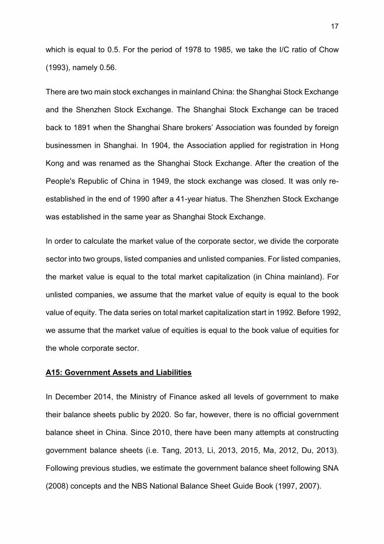
3. Estimating market value (MV) equity of corporate sector. We estimate the MV

equity of listed companies (LC) and unlisted companies (ULC) separately. For listed

companies, the market value is equal to the total market capitalization (in China

mainland). For unlisted companies, we assume that the market value of equity is

equal to its book value. The data series on total market capitalization start in 1992.

Before 1992, we assume that the market value of equities is equal to the book value

of equities for the whole corporate sector.

4. Estimating public, private, and foreign share of MV and BV equity of listed

companies (LC). We estimate public, private, and foreign share of MV equity of

listed companies (LC) by combining the data from “China Financial Stability Report”,

Flow of Funds, and International Investment Position. Especially for MV private

capital

5. Estimate Private share of market value corporate equity

Private Share of MV Corporate Equity

= 𝑀𝑉 𝑜𝑓 𝑃𝑟𝑖𝑣𝑎𝑡𝑒 𝐶𝑎𝑝𝑖𝑡𝑎𝑙 𝑜𝑓 𝑈𝐿𝐶+𝑀𝑉 𝑜𝑓𝑃𝑟𝑖𝑣𝑎𝑡𝑒 𝐶𝑎𝑝𝑖𝑡𝑎𝑙 𝑖𝑛 𝐿𝐶𝑀𝑉 𝑒𝑞𝑢𝑖𝑡𝑦 𝑜𝑓 𝑈𝐿𝐶+𝑀𝑉 𝑒𝑞𝑢𝑖𝑡𝑦 𝑜𝑓 𝐿𝐶

=𝑃𝑟𝑖𝑣𝑎𝑡𝑒 𝑠ℎ𝑎𝑟𝑒 𝑜𝑓 𝑈𝐿𝐶 ∗ 𝑀𝑉 𝑒𝑞𝑢𝑖𝑡𝑦 𝑜𝑓 𝑈𝐿𝐶 + 𝑃𝑟𝑖𝑣𝑎𝑡𝑒 𝑠ℎ𝑎𝑟𝑒 𝑜𝑓 𝐿𝐶 ∗ 𝑀𝑉 𝑒𝑞𝑢𝑖𝑡𝑦 𝑜𝑓 𝐿𝐶

𝑀𝑉 𝑒𝑞𝑢𝑖𝑡𝑦 𝑜𝑓 𝑈𝐿𝐶 + 𝑀𝑉 𝑒𝑞𝑢𝑖𝑡𝑦 𝑜𝑓 𝐿𝐶

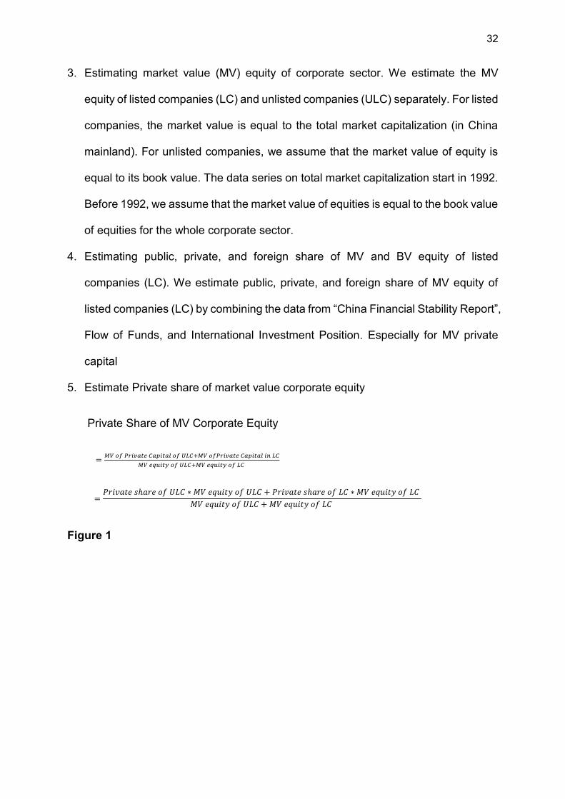
Figure 1

33

Source:

PYZ2017NationalAccountData

Figure 1 shows the market value of private share of unlisted companies, listed

companies and the corporate sector (both unlisted and listed companies). The “bump”

is caused by the decreasing share of private capital in LC during Chinese stock bubble

in 2007. All raw data and estimation are included in excel appendix file

“PYZ2017NationalAccounts”.

C. Comparison

There is a difference in the 2004 public share reported in our paper (63%) and in the

government report “The First National Economic Census Key Gazette (No. 1) 2004

(56%)”. However, in the end we decided to use our estimation instead of the one in

NBS report. For detailed reasons please see below.

Since “The First National Economic Census Key Gazette (No. 1) 2004” (2004 CKG)

did not explain how the public share is calculated calculates, we could not know exactly

what the causes are for the difference between two estimations of public share.

However, after carefully comparing the data from 2004 CKG and National Economic

Census Yearbook 2004 (2004 NECY), we believe the difference in two public share

0%5%

10%15%20%25%30%35%40%45%

Private Share

MV_ULC MV_LC MV_ULC&LC

34

estimations can be explained by the inconsistent sample coverage between national

level statistics and industrial level statistics published by NBS in 2004 CKG and 2004

NECY.

More precisely, in both 2004 CKG and first volume of 2004 NECY (which reports the

national level economic census statistics), the sample covers 5,168,303 legal person

units, including 6,823,994 active units (one corporative enterprise can have more than

one active unit). Especially, in industry sector (mining industry, manufacturing,

electricity, gas and water production and supply industry), it covers 1,525,901 active

units in industry

However, in the second volume of 2004 NECY (which reports industrial level economic

statistics), the sample of Industry sector (Mining Industry, Manufacturing, Electricity,

Gas and Water Production and Supply Industry) only covers 1,375,263 active units.

There are 150,638 active units (around 10% active units) missing comparing to 2004

CKG and first volume of 2004 NECY. The same inconsistency also happens in

construction and real estate sector.

As we explained before, in our research we estimate national level paid in capital and

ownership structure of corporate sector based industrial level data from the second

volume of NECY. Thus, our estimations are based on a sample with less LP units

(active units) than 2004 CKG.

Meanwhile, in 2004 CKG, the total paid in capital is 18.2 trillion RMB, while our

estimation is 16.8 trillion RMB, which is 7.5% short. This difference is also due to the

difference of the coverage of the sample.

Since on average private owned corporates are much smaller than public owned

corporates and their financial reports are more likely to be incomplete, thus they will

35

be more likely to be “missed”. Thus, as a robustness check, we assume missing legal

person units are all private owned corporates and add their missing paid in capital

(18.2-16.8=1.4 trillion RMB) back to the private capita, then new estimated public share

is 55% in 2004, which is very close to the result reported in 2004 CKG (56%).

Despite the gap between our estimation and NBS report in 2004 CKG, we choose our

method rather than NBS estimation instead, because

1. With our method, we are able to decompose corporate balance sheet by industry.

Thus, we are able to estimate the paid in capital, but also assets and liabilities of

corporations for each industry. 2004 CKG only report the amount of total paid in

capital in corporate sector without any further information on assets and liability.

2. Instead of taking results directly from NBS report in 2004 CKG, we provide detailed

and transparent estimation process based on more detailed data in our appendix

file “PYZ2017NationalAccounts”, so that it could be improved once new data is

available.

3. The ownership structure of legal person units is only reported in 2004 CKG for

Economic Census 2004. There is no similar statistics reported for Economic

Census 2008 and 2013. Although we analyze the potential cause for the different

estimation of public share in our research and 2004 CKG, without NBS explaining

its detailed calculation method, we are not able to make any conclusion and make

corresponding “correction” for Economic Census 2008 and 2013. Thus, to be

consist and more accurate, we choose to use industrial level statistics and the same

method for all three Economic Censuses.

36

A2: National Income Series

A21: Real GDP and National Income

There has been considerable debate about the real growth of China over the last

decades and the extent to which it is over-estimated by official statistics. The need for

adjusting the official estimates is acknowledged by government statisticians (see Xu

and Ye, 2000, pp. 16–17):

“… the sheer size of China, together with the limited resources currently devoted to

national accounts and the continuation of MPS [material planning system]-oriented

statistical procedures, inevitably means that the official GDP estimates are subject to

margins of error that are somewhat bigger than for other developing countries and

substantially larger compared with most other OECD countries.”

A lot of work has been devoted to identifying data problems in the official statistic and

proposing alternative estimates. There are two different approaches in the literature

to correct official real GDP growth. The first approach corrects real growth rate by re-

estimating volume changes in the economy. Maddison and Wu estimate gross value

added by output sectors. Maddison (1998) re-estimated gross value added in farming

and “non-material services” and Wu (1997) estimated gross value added in industry by

constructing a volume index (see also Maddison, 2009, Wu, 2002, 2011, Maddison

and Wu 2008). Rawski (2001) revised the GDP growth rate of China using energy

consumption. The second approach adjusts real growth rate by re-estimating the GDP

deflator and use the alternative deflator to deflate official nominal GDP figures (see,

Woo 1998, Ren, 1997 and Young, 2003).

37

In our study, we re-estimate real GDP growth using the second approach. We replicate

the carefully documented method of Young (2003) to construct an alternative GDP

deflator. There are two reasons why we chose to do so. First Young (2003) uses

sectoral price indices from the published national accounts, so the construction of his

price index can be exactly replicated. By contrast, Maddison and Wu rely on a mixture

of official (but not necessarily public) sources and more subjective adjustments.

Second, for internal consistency we prefer to stick to the official national accounts,

making well documented adjustments when needed, rather than disregard the national

accounts series altogether in favor of external sources.

The GDP growth rate we obtain – by following Young (2003) – lies in between the

official GDP growth rate and the one estimated by Maddison-Wu, but it is closer to

Maddison-Wu. This result is consistent with the view of Chinese government

statisticians, according to whom: “A reasonable assessment might be that the official

growth estimates represent an upper bound and the Maddison estimates a lower

bound, with the true growth rates lying somewhere between the two” (see Xu and Ye,

2000, pp. 16–17). For further details on the construction of our deflator, see Appendix

PZY2016NationalAccountData, Table AP11.

Moreover, we also increase the level of GDP by including housing rental income in

GDP. As explained in NBS’s GDP guide book (Xu et al. 2007, pp. 83), in the official

statistics, the gross output of owner-occupied housing is set equal to the value of the

intermediate goods (utilities) and services consumed plus the consumption of fixed

capital. This means that the net value added of owner-occupied housing is equal to 0.

By doing so, the official statistics underestimate national income. In our study, we

assume that the net value added of owner-occupied housing is equal to 2% of the

market value of housing – and we increase national income accordingly.

38

A22: Capital Depreciation

We estimate national-level capital depreciation using Input-Output tables. NBS has

been publishing China’s IO table since 1987, so far there have been 10 IO tables

released. IO tables report national value added and depreciation of fixed assets, that

we use to calculate national capital depreciation rates. For details, see

“PYZ2017NationalAccountData”, Table AP1.

A23: Flow of Funds

Since NBS started compiling Flow of Funds (FOF) in 1992, there has been two

revisions. The first revision occurred in 2008, when NBS revised FOF for the period of

1992-2004 based on the first China Economic Census (2004). The revised FOF tables

are published in “Flow of Fund Historical Materials (1992-2004)”. The second revision

occurred in 2012, when NBS revised the FOF for the period 2000-2009 based on new

published government revenue data and revised Balance of Payment. The revised

FOF is published in China’s Statistic Yearbook 2012.54

The FOF data we use come from two sources: 1) for the 1992-1999 period, the FOF

is from “Flow of Fund Historical Materials (1992-2004)”; 2) for the 2000-2014 period,

the FOF is from China Statistic Yearbook (2012-2016).

Saving

In the Flow of Funds, we have the following accounting identity:

Value Added - Capital Depreciation + Net Compensation of Employees + Net Taxes on Production + Net Income from Property

54 FOF (1992-1999) is still under revision (China Statistic Yearbook, 2012)

39

+ Net Current Transfer - Consumption = Net Saving

For the household and government sectors, saving can be divided into net non-

financial assets saving, net financial assets saving, and net capital transfers. In the

corporate sector (retained earnings), we divide saving into private saving, public saving,

and foreign saving based on the share of corporate equities owned by the private,

public, and foreign sectors.

Capital Income

We divide capital income into two part, operating surplus (including housing rents) and

net income from property.

Value added – Capital Depreciation + Net Compensation of Employees + Net Taxes on Production =Operating Surplus (Including Housing Rents)

Net Interest + Net Distributed Income of Corporations + Net Rent on Land + Net Other Income from Properties. =Net Income from Property

Regarding the mixed income in household sector, in China’s GDP accounting,

operating surplus and compensation of individual business owners are both treated as

operating surplus, the compensation of individual business only includes employee’s

compensation. Moreover, operating surplus and compensation of farmers are both

treated as compensation. 55

55 NBS’s GDP guide book (Xu et al. 2007, pp. 11)

40

In order to split mixed income to compensation of employee and operating surplus, in

this research we assume:

For individual business,

Operating Surplus = (Value added- Capital Depreciation- Production Tax) * 5%

Compensation of Employee = (Value added- Capital Depreciation- Production Tax) *

95%

For farmers,

Operating Surplus = (Value added- Capital Depreciation- Production Tax) * 30%

Compensation of Employee = (Value added- Capital Depreciation- Production Tax) *

70%

A24: Public Revenue

Following Naughton (2017), we estimate public revenue in China for the period from

1992 to 2015, see Appendix Table A313. However, our estimates of public revenue

are higher than Naughton (2017) due to three reasons.

a. We include off-budget revenue in “Total Fiscal Revenue”. Off-budget revenue

are the government revenue that are not included in the annual budget or are

not subject to the same general level of reporting, regulation, or audit as other

public finance items. They include fees charged by administrative and

institutional units, SOEs’ after tax profits,56 revenue and additional incomes of

56 83 administrative fees have been included into government budget since 1993. SOEs’ profit were excluded from off-budget management in 1993 “Provisions on budget management for administrative fees and fines” (COCC [1993] No. 19)

41

government managed funds57, self-financing funds for township government

expenditure, etc. Since 2011, all off budget revenues are included into

government budget.58

b. In addition to land revenue, we also include the revenue from government-

managed funds, such as, Railway Construction Fund, Local education

Surcharges, Financial Revenue from Central Special Debt Management,

Lottery Proceeds, Urban Infrastructure Supporting Fees, Tolls etc.

c. For the public share of corporate undistributed profit, out estimates are higher

than Naughton’s, especially in the early years. This is because Naughton only

includes enterprises solely funded by the State and State-holding enterprises in

his estimate, while we estimate the public share of corporate undistributed

profits by splitting the retained earnings of the whole corporate sector between

the public and private sectors based on their respective equity shares.

We find that total fiscal revenue increased from 22% of national income to 39% of

national income from 1992 to 2015, while total public revenue increase from 31% to

49% during the same period. For more details, see Appendix please see Appendix

(PZY2016NationalAccountData, AP11).

57 In 1996, 13 government managed funds were included in to government budget. “Decision on Strengthening the Management of Off-budgetary funds” (SC [1996] No. 29) 58 “Notice of Ministry of Finance regarding Including Income of Off-budget Funds into the Budget Management” (FB [2010] No. 88)

42

Appendix B. Income and wealth distribution series

B1. Benchmark distribution series and variants

B2. Comparisons with other distribution series

B3. Differences between wealth surveys

B4. Income concepts used in income tax data and surveys

43

Appendix B. Income and wealth distribution series

Our detailed income and wealth distribution series are given in the zipped directory

PYZ2017DistributionSeries.zip. This directory includes our final benchmark

distribution series PYZ2017FinalDistributionSeries.zip, as well as alternative series

and the complete computer codes and all detailed computations that we used to

construct these series. For more details on the organization of these files, see

ReadMePYZ2017DistributionSeries.doc.

In addition, the zipped directories PYZ2016IncomeDistributionData.zip and

PYZWealthDistributionData.zip include detailed raw data and files from household

income survey, income tax tabulations, and household wealth surveys and billionaire

rankings.

B1: Benchmark estimates and variants

The general methodology that we use in order to construct our income and wealth

distribution series is described in the main paper (section 2.2). It basically consists of

three steps: in step 1 we use raw household income survey tabulations and

generalized Pareto interpolation techniques59 in order estimate raw series on the

distribution of raw survey income and raw fiscal income by g-percentile (before any

correction); in step 2 we use high-income-taxpayers income tax data in order to correct

upwards these estimates and obtain corrected estimates of the distribution of fiscal

59 Generalized Pareto interpolation allows for the recovery of the distribution based on income tabulations without the need for parametric approximations. This method has demonstrated its ability to produce very precise results and also has the advantage of generating smooth estimates of the distribution, i.e. generating a differentiable quantile function and a continuous density, while other methods introduce kinks around the thresholds used as inputs for the tabulation. For more details please see Blanchet, Fournier and Piketty, 2017. The generalized Pareto interpolation procedure (available online at www.wid.world/gpinter) generates 127 generalized percentiles, namely p0p1, p1p2, ..., p99p100, corresponding to 100 fractiles of the distribution. The top fractile is split into 10 deciles (p99.0 p99.1, p99.1 p99.2,..., p99.9p100), its top decile itself split in ten deciles (p99.90 p99.91, p99.91 p99.92, ..., p99.99 p100), the tenth decile again split in ten deciles (p99.990p99.991, p99.991 p99.992, ..., p99.999p100). The top generalized percentile thus corresponds to the top 0.001% of the population.)

44

income by g-percentile; in step 3 we use national accounts and wealth data in order to

include tax-exempt capital income data (such as undistributed profits, imputed rent and

other “non-fiscal income”) and to obtain corrected estimates of the distribution of pre-

tax national income by g-percentile. All details are provided in the data files and

computer codes. Here we discuss a number of additional issues about variant series

and robustness checks.

The impact of our two corrections – the fiscal-data correction and the wealth-data

correction – is summarized on Figures B1-B2 (extracted from file China_y.xlsx). As

one can see, the fiscal-data correction is quantitatively more significant than the

wealth-data correction. Note however that the latter becomes larger at the very end of

the period, first because of the larger macroeconomic magnitude of non-fiscal income

(rising importance of privately-owned undistributed profits and imputed rent), and next

– and most importantly – because of rising concentration of private property. We report

on Figures B3-B4 (extracted from ChinaUrban_y.xlsx) the impact of the two corrections

for urban China only. The magnitude of the corrections are approximately the same for

urban and rural China, to a large extent by construction (see below). We deal with each

of the two corrections in turn.

B11: Fiscal data correction

Regarding the fiscal-data correction, we choose in our benchmark series to apply the

same average upgrade factors by g-percentiles (estimated using national fiscal data

available over the 2006-2010 period) to the entire 1978-2015 period. By doing so, it is

possible that we under-estimate the rising inequality trend over the 1978-2015. On the

other hand, it would clearly be unjustified not to upgrade at all the self-reported survey

data at the beginning of the period (which indicates extremely low levels of inequality).

In the absence of adequate tax tabulations prior to 2006, assuming constant

45

proportional upgrade factors throughout the period seems like the most justified

assumption (this is also consistent with the findings by Piketty-Qian 2009 showing an

approximately stable gap between survey-predicted and actual income tax revenues).

For the same reason, we also apply the same proportional upgrade factors by g-

percentile to rural income survey data as those estimate for urban China using fiscal

data. The fact that rural incomes are for the most part not subject to income tax does

not imply that self-reported rural incomes are not under-estimated: we observe a

downward bias in self-reported incomes at the top of the distribution in all household

surveys at the international level, and there is no evidence suggesting that the bias is

generally different in rural areas as in urban areas. As a first approximation, and in the

absence of other information, the most justified assumption seems to be to apply the

same proportional upgrade factors by g-percentile to rural incomes as those estimated

for urban incomes.

We also report in the data files variant estimates using yearly variations in national

fiscal data correction factors for years 2006-2010, as well as provincial fiscal

tabulations for years 2011-2015 (see figures in ChinaUrban_yf.xlsx). However at this

stage available yearly variations in tax data – particularly at the provincial level – seems

too incomplete and fragile to be used in our benchmark series.

The way we estimate our upgrade factors is described in a detailed manner in the file

ChinaUrban_yf_raw.xlsx (sheets CompUpgradeFactors and UpgradeFactors). There

are two important issues here. One is about the differences in income concepts and

the ratio between post-deductions taxable income and pre-deductions fiscal and

survey income. The second issue is about the profile of upgrade factors.

46

We start with the first issue. As explained in the DINA Guidelines (Alvaredo et al 2016),

it is critical to be very precise about income concepts when using income tax data and

combining it with survey data. In particular, income tax tabulations – in China and in

most other countries – are usually based upon some form of “taxable income” concept

(i.e. income subject to income tax, after a number of deductions allowed by tax

legislation). These deductions can be very extensive: e.g. in China they typically

include deductions for a large number of compulsory and/or voluntary contributions to

pension funds, health insurance plans, housing funds (the corresponding benefits are

generally not subject to tax); in some other countries they sometime include large

proportional or lump-sum deductions for professional expenses, previous-year-taxes,

etc., so that taxable income can be significantly smaller than “fiscal income” (which we

define as the sum of all income items legally subject to taxation, before any deduction;

see Alvaredo et al 2016).

In the case of China, given the existing deduction rules, we assume in our benchmark

estimates that the ratio between taxable income and fiscal income is equal to r=80%,

and is approximately constant across income levels (see section B.4 below for

additional details on the differences between the income concepts used in income tax

data and household surveys; see file PYZ2017DistributionalData.xlsx, sheet

TaxablevsFiscalIncome for detailed computations). We also provide as robustness

checks a number of variant estimates using other ratios (in particular r=70% and r=90%)

(see ChinaUrban_yf_raw.xlsx, sheets CompUpgradeFactors and UpgradeFactors).

Given the very large ratios between fiscal income and survey income at the level of

very top percentiles (around 250%-300%, see below), this has a relatively limited

impact on our final estimates.

47

We now come to the second issue, i.e. the profile of upgrade factors. As discussed in

the main paper (section 2.2), the ratios between fiscal and survey incomes fall in the

1.3-1.6 range if we look at the quantile function q(p) (i.e., the income threshold q(p)

corresponding to percentile p = 0.995) and in the 2.5-3 range when we look at the

upper incomes y(p) (i.e., the average income y(p) above percentile p = 0.995). In other

words, top incomes are massively underestimated in the survey as compared to fiscal

data.60 Our benchmark correction is based upon the following assumption: the survey

data is reliable below percentile p1 = 0.8, the fiscal data is reliable above p2 = 0.995,

and we assume that the quantile ratio upgrade factor f(p) rises piecewise-linearly from

f(p1) = 1 to the observed fiscal/survey ratio f(p2) between p1 and p2, with a small and

rising slope between p1 = 0.8 and p=0.9 and a constant linear slope between p=0.9

and p2 = 0.995.

We also provide as robustness checks a number of variant estimates using other

profiles for the curve f(p) (see ChinaUrban_yf_raw.xlsx, sheets CompUpgradeFactors

and UpgradeFactors). In particular, we consider a profile where we assume the survey

data to be reliable below percentile p1 = 0.9, the fiscal data to be reliable above

p2 = 0.995, and a linear profile of f(p) between p1 and p2. Yet in other profiles we

assume a convex (increasing slope) or concave (declining slope) of f(p) between p1

and p2. Unsurprisingly, the more the rising part of the f(p) profile is pushed toward p2,

the smaller the total upgrade to the top 10% share; and the more the rising part of f(p)

is pushed toward p1, the larger the total upgrade to the top 10% share. As long as we

do not have access to income tax data covering the entire top 10% (rather than merely

the top 1% or top 0.5%), we have no way to be sure about this. However, our variant

60 In particular, the inverted Pareto coefficient b(p)=y(p)/q(p) is as low as 1.5 or less in the survey, as opposed to 2.5-3 or more in the tax data.

48

estimates show that the total impact of the top 10% share is relatively limited in any

case, because in practice most of the adjustment comes from the top 1% share (see

Figures B1 to B4 above; see

ChinaUrban_yf_raw.xlsx, sheets CompUpgradeFactors and UpgradeFactors). The

main reason for the benchmark assumptions described above is that they lead to a

smooth and convex profile of inverted Pareto coefficients b(p) (see Figure B5), in line

with what we find in countries with high-quality fiscal data (see Blanchet, Fournier and

Piketty, 2017). Other profiles tend to lead to not-well-behaved (non-convex and/or very

steep) Pareto curves.

B12: Wealth data correction

We now come to the wealth-data correction. As explained in the main paper (section

2.2), there are three steps here. First, we correct the wealth distribution using Hurun

Rich Lists. As explained in the paper, to measure the wealth inequality, we use the

CHIP household wealth surveys conducted in 1995 and 2002, and the CFPS

household wealth surveys conducted in 2010 and 2012.61 Since it is always a challenge

to reach out to very wealthy individuals in surveys, it is likely that they under-estimate

top wealth levels. We therefore combine the wealth surveys with the data from the

annual Hurun rankings of China’s wealthiest households covering the 2001-2016

period. We apply generalized Pareto interpolation techniques to the combined data to

produce complete wealth distribution series.

Our benchmark correction is based upon the following assumption: the survey data is

reliable below percentile p1 = 0.90, the Hurun Rich List is reliable above p2 = 99.999%

61 CHIP surveys were also conducted in 2008 and 2013, but these two survey years raise difficulties, so we do not use them (the 2008 survey had problems with the sampling process and is considered not to be nationally representative, and the 2013 survey has no information on housing values).

49

(for example, in 2001, p2= 99.999973%, 2012, p2= 99.999509%, in 2015 p2=

99.999033%). We combine these two series, then apply an upgrade factor to the

quantile function q(p) (i.e., the income threshold q(0.995) corresponding to percentile

p = 0.995) between p1 and p2.

For the variants of upgrade factor, we have applied upgrade factor=1, 1.1, 1.2….262

(see Appendix Figures B. 12a - B. 12b). As benchmark correction, we choose upgrade

factor=1.5 for year 1995, 2002, 2010, and 2012 (see WealthTabulations2002Variant

and WealthTabulations2012Variant for different variants of upgrade factor), since by

applying the upgrade factor=1.5 in our benchmark distribution, our estimation of top

10% wealth share in 2012 is consistent with Li and Wan (2013) and Xie and Jin (2015).

For the year from 2003 to 2009, we first estimate the wealth distribution using adjusted

wealth survey tabulations of 2002 based on national incomes, then corrected top

income share using yearly Hurun Rich List data. The same procedure is applied for the

year from 2011, 2013, 2014 and 2015 using wealth survey tabulation of 2012. (see

BenchmarkWealthTabulations).

Second, using the national accounts we estimate the evolution of total non-fiscal

capital income ynf, which we define as the private share of undistributed profits and

other tax-exempt capital income flows (including imputed housing rent) accruing to

Chinese households. We find that ynf gradually rises from less than 5% of per adult

national income to as much as 15% over the 1978-2015 period (with a peak in 2007,

and a decline to about 11-12% in recent years), largely due to the rise of private

corporate ownership and private housing. In contrast, total fiscal income yf (i.e., total

income subject to income tax, before any deduction) represents approximately 70% of

62 For year 2002 and 2012, if upgrade factor>2, then average survey wealth per adult is bigger than average wealth per adult calculated based on national accounts.

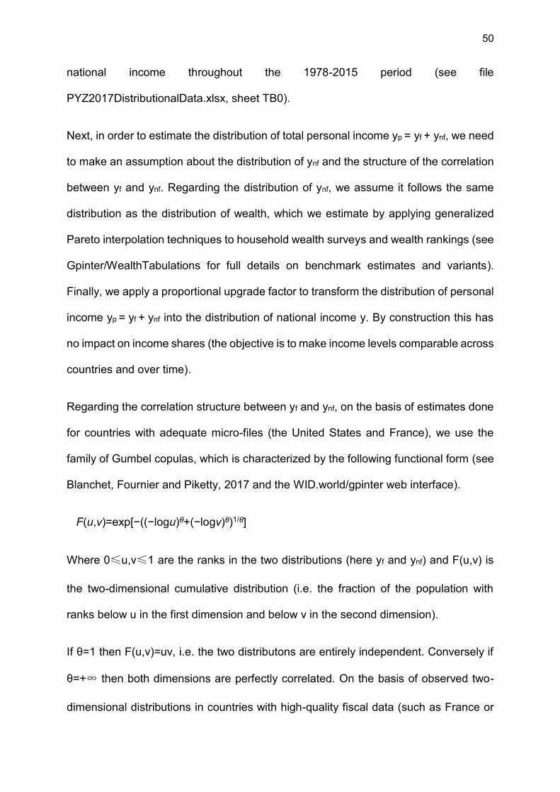
50

national income throughout the 1978-2015 period (see file

PYZ2017DistributionalData.xlsx, sheet TB0).

Next, in order to estimate the distribution of total personal income yp = yf + ynf, we need

to make an assumption about the distribution of ynf and the structure of the correlation

between yf and ynf. Regarding the distribution of ynf, we assume it follows the same

distribution as the distribution of wealth, which we estimate by applying generalized

Pareto interpolation techniques to household wealth surveys and wealth rankings (see

Gpinter/WealthTabulations for full details on benchmark estimates and variants).

Finally, we apply a proportional upgrade factor to transform the distribution of personal

income yp = yf + ynf into the distribution of national income y. By construction this has

no impact on income shares (the objective is to make income levels comparable across

countries and over time).

Regarding the correlation structure between yf and ynf, on the basis of estimates done

for countries with adequate micro-files (the United States and France), we use the

family of Gumbel copulas, which is characterized by the following functional form (see

Blanchet, Fournier and Piketty, 2017 and the WID.world/gpinter web interface).

F(u,v)=exp[−((−logu)θ+(−logv)θ)1/θ]

Where 0≤u,v≤1 are the ranks in the two distributions (here yf and ynf) and F(u,v) is

the two-dimensional cumulative distribution (i.e. the fraction of the population with

ranks below u in the first dimension and below v in the second dimension).

If θ=1 then F(u,v)=uv, i.e. the two distributons are entirely independent. Conversely if

θ=+∞ then both dimensions are perfectly correlated. On the basis of observed two-

dimensional distributions in countries with high-quality fiscal data (such as France or

51

the US), we find that Gumbel parameters are typically in the 2-4 range. We use θ=2

for our benchmark simulations, as it is the lower bound of the income inequality

estimation using different Gumbel parameters. However, the important point is that this

has relatively small impact for our final series, as is clearly illustrated by the variant

estimates with different Gumbel parameters (see Appendix Figures B. 8e to B. 8h).

Intuitively, what really matters for the concentration of the sum yp = yf + ynf is, first, the

fact that the concentration of non-fiscal income ynf (i.e. the concentration of wealth) is

much larger than the concentration of fiscal income yf , and next the macroeconomic

importance of the non-fiscal income component (i.e. whether it provides an additional

income of 10%, 30% or 50% as compared to fiscal income). For a given

macroeconomic significance of ynf (say, around 11-15% of national income), and for a

given gap between the concentration of yf and ynf, the fact that the Gumbel parameter

θ is equal to 2.5, 3 or 3.5 (or even 1.5 or 5) has relatively limited implications (see

Appendix Figures B. 8e to B. 8h).63

Finally, we should stress two additional limitations of our estimates. First, due to lack

of data before 1995, our wealth distribution series start only in 1995. In order to perform

the Gumbel copula estimates for the 1978-1994 sub-period, we simply assumed the

same wealth distribution as for 1995 (with adjustment for average wealth series). This

assumption is acceptable for the distribution of pre-tax national income (especially

given the limited importance of non-fiscal income at the beginning of the period).

However, it implies that wealth distribution series should only be used for the post-

1995 period.

63 We do not show the simulations for θ=2.5 or 3.5 on Appendix Figures B. 8e to B. 8h because they would be virtually undistinguishable from θ=3.

52

Next, we should make clear that our separate distributional series for urban and rural

China are not fully satisfactory. In effect, we have separate raw data for urban and rural

China only for household income surveys. For national accounts data, as well for

income tax data and for wealth data (wealth surveys and Hurun billionaire rankings),

we only have data for total China. So we just assume same fiscal-data correction for

urban and rural incomes, the same average wealth urban/rural ratio as for survey

income, and the same wealth distribution for urban and rural as for total China. This

implies for instance that merging the urban and rural distributions of pre-tax national

income for urban and rural China (using the “merge countries” option in

wid.world/gpinter) does not lead exactly to the total China estimates. This is one of the

many directions in which our series ought to be improved in the future, ideally by using

more detailed data sources on inequality at the provincial level (rather than simply at

the level of urban vs rural China).

53

B2: Comparison with Other Distribution Series

B21: NBS vs. CHIP

Here we provide additional details about the comparison between our survey data

source (NBS survey tabulations) with China Household Income Project (CHIP), one of

the most commonly used surveys in China inequality studies.

First, we compare the distribution of income in the NBS tabulations and the CHIP

micro-data. The results are reported in the Appendix Table S2. We find that the

distribution of income is virtually identical in both datasets. For instance, the bottom

50% income share is 29% in the NBS tabulations vs. 27% in the CHIP micro-data in

2012; the middle 40% income share is 47% in both datasets in 2012; the top 10%

income share is 24% in the NBS tabulations vs. 26% in the CHIP micro data. This

validates the reliability of the generalized Pareto-interpolation techniques of Blanchet,

Fournier and Piketty.

Second, we compare the distribution of income in the CHIP microdata and in our series

that combine NBS tabulations and fiscal data. We focus the comparison on the bottom

80% of the distribution, since we assume that survey data are accurate for the bottom

80%. The results are presented in the Appendix Figures B.11a to B.11h. These figures

show that the distribution of income within the bottom 80% in the CHIP micro-data and

in our series is very close. For instance, the bottom quartile (of the bottom 80%) earns

16% of total income (of the bottom 80%) in the CHIP survey vs. 18% in our series in

2012. The second quartile earns 30% of income in the CHIP survey, just as in our

series. The top 30% earns 54% of income in the CHIP survey vs. 53% in our series.

This comparison is summarized in a Appendix Table S2.

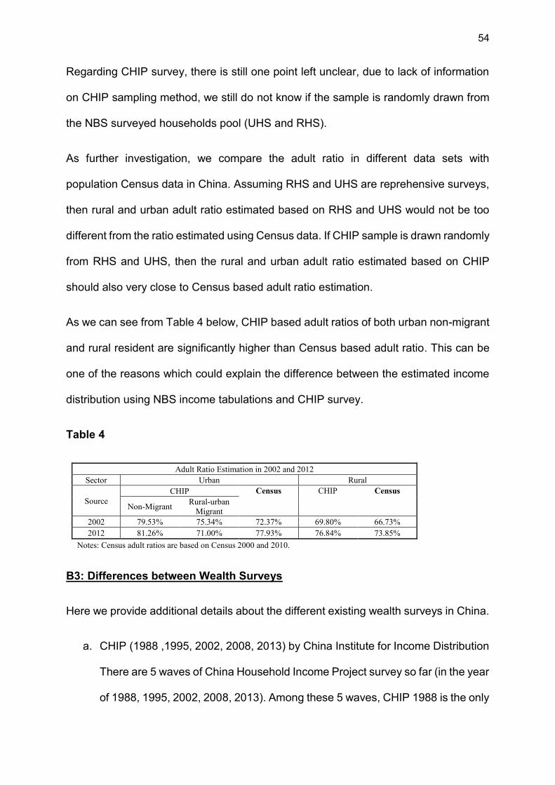
54

Regarding CHIP survey, there is still one point left unclear, due to lack of information

on CHIP sampling method, we still do not know if the sample is randomly drawn from

the NBS surveyed households pool (UHS and RHS).

As further investigation, we compare the adult ratio in different data sets with

population Census data in China. Assuming RHS and UHS are reprehensive surveys,

then rural and urban adult ratio estimated based on RHS and UHS would not be too

different from the ratio estimated using Census data. If CHIP sample is drawn randomly

from RHS and UHS, then the rural and urban adult ratio estimated based on CHIP

should also very close to Census based adult ratio estimation.

As we can see from Table 4 below, CHIP based adult ratios of both urban non-migrant

and rural resident are significantly higher than Census based adult ratio. This can be

one of the reasons which could explain the difference between the estimated income

distribution using NBS income tabulations and CHIP survey.

Table 4

Adult Ratio Estimation in 2002 and 2012 Sector Urban Rural

Source CHIP Census CHIP Census

Non-Migrant Rural-urban Migrant

2002 79.53% 75.34% 72.37% 69.80% 66.73% 2012 81.26% 71.00% 77.93% 76.84% 73.85%

Notes: Census adult ratios are based on Census 2000 and 2010.

B3: Differences between Wealth Surveys

Here we provide additional details about the different existing wealth surveys in China.

a. CHIP (1988 ,1995, 2002, 2008, 2013) by China Institute for Income Distribution

There are 5 waves of China Household Income Project survey so far (in the year

of 1988, 1995, 2002, 2008, 2013). Among these 5 waves, CHIP 1988 is the only

55

one that does not contain wealth data, the rest contain not only income data but

also wealth data.

All the CHIP waves contain surveys of urban and rural households. In view of

the increased importance of rural-to-urban migration, and because the urban

and rural household subsamples do not adequately cover migrants, the 2002

survey added a survey of rural-to-urban migrants.

The basic structure of CHIP survey is

1. Urban: Individual income survey and Household wealth survey

2. Rural: Individual income survey and Household wealth survey

3. Immigration survey

The samples in CHIP (1988, 1995, 2002, 2013) surveys were drawn from the

large sample used by the National Bureau of Statistics (NBS) in its annual

household survey, Urban Household Survey (UHS) and Rural Household

Survey (RHS).

“The samples in the 1995 and 2002 (CHIP) surveys were drawn from the large

sample used by the National Bureau of Statistics (NBS) in its annual household

survey.” (Li and Zhao, 2008)

“the sample of CHIP 2013 is coming from the big sample of the annual

integration household survey sample of NBS in 2013. The latter contains 160

thousand households in 31 provinces. The CHIP sample was selected by

systematic sampling method in three layers of east, center and west and

contains 15 provinces, 126 cities, 234 counties, 18948 households and 64777

individuals. In which, there are 7175 urban households, 11013 rural households,

and 760 migrant households.”64 However, in the household wealth survey of

64 See CHIP 2013 introduction, http://www.ciidbnu.org/chip/chips.asp?year=2013

56

CHIP2013, the value of the house is not reported, so we are not able to use this

survey in our research.

CHIP 2008 is different from other CHIP surveys, it is a part of the larger RUMiC

(Rural-Urban Migrants in China) survey project. The sampling procedure and

survey method for the 2008 migrant survey were described in detail in the Rural-

Urban Migration in China Project Survey Documentation. See Sherry Tao Kong

(2010). CHIP2008 contained 5000 households in migration sample, 8000

households in rural sample and 5000 households in urban sample. Urban

sample was interviewed with questionnaires designed by the project team. The

problem with CHIP 2008 is that the weight variable is not released, thus the

estimation based unweighted CHIP 2008 could be inconsistent. In our research

we excluded CHIP 2008.

b. CFPS (2010, 2012) by Beijing University

China Family Panel Study is similar to CHIP but conducted by Beijing University.

It contains the national survey on income and wealth. For details, please see

http://www.isss.edu.cn/cfps/EN/

57

B4: Income Concepts Used in Income Tax Data and Household Surveys

Here we provide additional information regarding the differences between the income

concepts used in income tax data and in household surveys. We start with the definition

of taxable income used in the circular about high-income taxpayers, and then compare

with the income concept used in household urban and rural surveys.

B.41: Income Concept for the Self-declaration of Individual Income Tax (Annual

Income Above 120,000 Yuan)

“Circular of the State Administration of Taxation Concerning Printing and Distributing

the Measures for the Self-declaration of Individual Income Tax (for Trial

Implementation)” (GS [2006] No.162)

Article 6

“The "annual income of 120,000 Yuan or more" as stipulated in the present Measures

means the total amount of the following items of income obtained by a taxpayer in a

tax year reaching 120,000 Yuan:

(1) Wages and salaries; (2) Income of production or business operation obtained by

self-employed industrial and commercial households; (3) Income from contractual or

leased operation of enterprises and institutions; (4) Remunerations for providing

services; (5) Author's remunerations; (6) Franchise royalties; (7) Interests, dividends

and capital bonuses; (8) Income from leasing property; (9) Income from transferring

property; (10) Contingent income; (11) Other taxable income determined by the public

finance department of the State Council. “

Article 7

58

“The "income" as stipulated above of the present measures does not include the

following kinds of income:

(1) Tax-exempt income: (a) awards for achievements in science, education, technology,

culture, public health, physical culture and environmental protection granted by

provincial people's governments, ministries and commissions under the State Council ,

the People's Liberation Army units at army level and above and by foreign or

international organizations; (b) interests accruing from national bonds and other

financial debentures issued by the state; (c) subsidies and allowances received under

the state uniform provisions namely, special government allowances, allowances for

academicians, allowances for senior academicians that are granted in accordance with

the provisions stipulated by the State Council as stipulated in Article 13 of the

Regulation concerning the Implementation of the Individual Income Tax Law, and other

kinds of subsidies and allowances that are exempt from individual income tax as

stipulated by the State Council; (d) welfare benefits, pensions for the disabled or for

the family of the deceased and relief funds; (e) insurance compensation; (f) military

severance pay and demobilization pay; (g) settling-in allowances, severance pay,

retirement wages, retirement wages for veteran cadres, and living subsistence

allowances for retired veteran cadres distributed to cadres and employees under the

state uniform provisions; (h) incomes of diplomatic representatives, consular staff and

other personnel of foreign embassies and consulates in China, which shall be exempt

from tax in accordance with the provisions of related laws of China; and (i) incomes

which shall be exempt from tax under the international conventions in which the

Chinese Government joins or agreements which the Chinese Government has signed.

59

(2) Incomes obtained from abroad which can be exempt from tax as stipulated in Article

6 of the Regulation concerning the Implementation of the Individual Income Tax Law;

and

(3) Basic endowment insurance premiums, basic medical insurance premiums,

unemployment insurance premiums and public accumulation fund for housing

construction paid by entities for their staff and individuals in accordance with the

provisions of the State as stipulated in Article 25 of the Regulation concerning the

Implementation of the Individual Income Tax Law.”

B42: Urban Household Survey Income

In urban household survey, total household income is classified into four categories:

employee income, business income, property income, and income of transfer. It

includes disposable income65, expenditure self-employment, the individual income tax,

the individual social security paid66 and bookkeeping subsides have been deducted.

Thus, the total income used in urban household survey is pre-tax after-replacement

income. For details please see “Introduction to Urban and Rural Household Surveys

of China” in “China Yearbook of Household Survey 2013”.

B43: Rural Household Survey Income

In rural household survey, net income (instead of total income) is used to measure

the household income. Net income refers to income of rural households in current

year from all sources after deducting expenditures. Net income is used mainly for

input in reproduction and consumption expenditure, and also in bank savings and

65 The sum total expenditures of final consumption, non-obligatory expenses and savings in a household. 66 the basic endowment insurance premiums, basic medical insurance premiums, and unemployment insurance premiums and public accumulation fund for housing construction paid by individuals (Three insurances and one fund).

60

non-committed expenses. “Per capita net income” reveals the level of average per

capita income in rural household. Its formula of calculation is:

Total income - Expenditure on household business - Tax payment - Depreciation on productive fixed assets - Transfer from rural friends and relatives = Net Income

Thus, the net income used in rural household survey is after-tax after-replacement

income.

In order to compare these the three incomes series, we have to make corresponding

adjustment.

B44: Adjustments between taxable income and housedhold survey income

The major difference between these two series is that in household survey income

include social security paid by household.

There are five social insurances and housing funding in the social security system of

China. These five insurances are pension, unemployment insurance, medical

insurance, work-related injured insurance, and maternity insurance. Pension,

unemployment insurance, and medical insurance are paid by employees and

employers together, while work-related injured insurance and maternity insurance are

only paid by the employers. 67

To be more precise, for pension, employers (companies, enterprises, etc.) are required

to pay 20% of total wage of its employee to pension fund (part of social security fund)

67 Owners of individual owned business can also join the social insurance system. For example, to join the pension fund system, they need to pay 18% of net profit every month to the pension fund.

61

every month. Meanwhile employees are also required to pay 8% of “base wage”68 to

pension fund every month. 69

For medical insurance, employees are required to pay 2% of his gross wage and per

month, which is saved into his personal medical insurance account. The employers

need to pay 6% of total wage of its employee, a part of which will be saved into its

employee’s personal medical insurance account (the percentage is depending on the

age of the employee), the rest will be saved into public medical insurance account. For

unemployment insurance, the employee pays 1% of his gross wage while the employer

pays 2% of the its employees’ gross wage. For work-related injured insurance, and

maternity insurance, only employers are required to pay 1% of its employee’s gross

wage for each insurance.

The housing fund are paid by both employer and employee, the rates are different from

city to city. It ranges from 10% to 40% of employee’s gross wage, splitting equally

between employer and employee. In our research, we assume the average is equal to

20%, thus employee will pay 10% of his gross wage to the housing fund.

68 The “base wage” is equal to employee’s wage when his wage is between 60%-300% of average wage in the province. If one’s wage is lower than 60% of average wage in the province, then 60% of average wage in the province will be used as his “base wage”; if one’s wage is higher than 300% of average wage in the province, then 300% of average wage in the province will be used as his “base wage” 69 Among the pensions paid by employers and employee, 11% of “base wage” will be saved into employee’s personal pension account, the left is saved into public pension fund. When one retires from his job, his pension is paid through both personal pension account and public pension fund.

62

Appendix C. Population Series

C1: Urban and Rural Population

Data of urban and rural population is from NBS. “Population data of 1981 and before

are from household registrations; for the year 1982,1990,2000 and 2010 are the

census year estimates; the rest of the data covered in those tables have been

estimated on the basis of the annual national sample surveys on population

changes.”

“The 4th National Census (1990) used the concept of permanent residence to

distinguish between rural and urban residents, by defining people who left their rural

home village and lived in an urban area for more than one year as permanent

residents of that urban area. After the Census was conducted, the National Bureau of

Statistics adjusted all data between 1982 and 1990 based on the measure of one-

year permanent residence. The 5th National Census (2000) shortened the

permanent residence to six months- namely, those rural migrants who had lived in

cities for more than six months were considered as permanent urban residents.

Among other new practices, this revised definition of urban residence substantially

enhanced the proportion of urban population in 2000, and accordingly and National

bureaus of Statistics, again, adjusted the data of urbanization between 1990 and

2000. Since then, urban population has been defined as people who have lived in an

urban area for more than six months, regardless where their residence is registered.”

(Yao & Wu, 2013)

63

References

Agarwala, M. (2012). Inclusive wealth report 2012 : measuring progress toward sustainability. Cambridge: Cambridge University Press.

Benjamin, D., Brandt, L., Giles, J., & Wang, S. (2005). Income Inequality During China’s Economic Transition. Working Papers.

F. Alvaredo, L. Chancel, T. Piketty, E. Saez, G. Zucman, "Distributional National Accounts (DINA) Guidelines: Concepts and Methods used in WID.world", WID.world Working Paper 2016/02

BCG. (2014). Developing Mixed Ownership Structures and Modern Enterprise Systems.

T. Blanchet, J. Fournier, T. Piketty, "Generalized Pareto Curves: Theory and Applications ", WID.world Working Paper 2017/03

Cao, Y., Zhong, H., Liao, S., & Ye, Q. (2012). Chongsu guojia zichan fuzhai nengli (Reconstruct the National Balance Sheet). Finance (Cai Jin), 15.

Chow, G. C. (1993). Capital Formation and Economic Growth in China. Quarterly Journal of Economics, 108(3), 809–842.

Cui, D. (1991). Research on China Urban Housing System Reform. Beijing: Finance and Economics Press.

Dean, R., & Damm-Luhr, T. (2010). A Current Review of Chinese Land-use Law and Policy: “A ‘Breakthrough’ in Rural Reform?” Pacific Rim Law & Policy Journal, 19(1), 121–159.

Edlund, L., Li, H., Yi, J., & Zhang, J. (2013). Sex Ratios and Crime: Evidence from China. Review of Economics and Statistics, 95(5), 1520–1534.

Gan, L., Yin, Z., Jia, N., Xu, S., Ma, S., & Zheng, L. (2013). Data you need to know about China: research report of China household finance survey 2012. New York: Springer.

Guo, Y., Gan, J., & Xu, C. (2008). A Nationwide Survey of Privatized Firms in China. Seoul Journal of Economics, 21(2), 1–21.

Hamilton, K. (2006). Where is the Wealth of Nations?: Measuring Capital for the 21st Century. Washington D.C.: World Bank.

Han, J., Liu, R., & Zhang, J. (2012). Globalization and wage inequality: Evidence from urban China. Journal of International Economics, 87(2), 288–297.

64

Hou, X. (1999). Wei you guang xia qian wan jian: Zhongguo cheng zhen zhu fang zhi du de zhong da tu po (Breaking Through of China Urban Housing Reform) (1st Edition). Guilin: Guangxi Normal University Press.

Holz, C. A. (2006). New capital estimates for China. China Economic Review, 17(2), 142–185.

Holz, C. A. (2014). The quality of China’s GDP statistics. China Economic Review, 30, 309–338.

Hsieh, C.-T., & Song, M. Z. (2016). Grasp the Large, Let Go of the Small: The Transformation of the State Sector in China. NBER Macroeconomics Annual, 30(1), 1–84. https://doi.org/10.1086/685949

Hsieh, C.-T., & Song, Z. (Michael). (2015). Grasp the Large, Let Go of the Small: The Transformation of the State Sector in China. Cambridge, MA.

Lee, A., Chua Janice, Leung Chris, Chow Nathan, Lo Lily, & Chui Lan. (2016). China: Accelerating SOE Reforms. Singapore.

Lee, J. (2009). State Owned Enterprises in China: Reviewing the Evidence.

Li, S., & Zhao, R. (2008). Changes in the Distribution of Wealth in China, 1995–2002. In J. Davies (Ed.), Personal Wealth from a Global Perspective (pp. 93–111). New York: Oxford University Press.

Li, Y. (2013). Zhongguo guo jia zi chan fu zhai biao 2013: li lun, fang fa yu feng xian ping gu (China National Balance Sheet: Theory, Method, and Risk assessment). Beijing: Zhongguo she hui ke xue chu ban she.

Li, Y., & Zhang, X. (2013). China’s sovereign balance sheet risks and implications for financial stability. In China’s road to greater financial stability (pp. 63–78). Washington, DC.

Li, Y., Zhang, X., & Chang, X. (2015). Zhongguo guo jia zi chan fu zhai biao 2015 : gang gan tiao zheng yu feng xian guan li (China National Balance Sheet: Leverage Control and Risk Assessment).

Ma, J., Zhang, X., & Li, Z. (2012). Zhongguo guo jia zi chan fu zhai biao yan jiu (A study of China’s national balance sheet). Beijing: Shehui Kexue Wenxian Chubanshe.

Maddison, A. (1998). Chinese Economic Performance in the Long Run. OECD Publishing.

Maddison, A. (2009). Measuring the Economic Performance of Transition Economies: Some Lessons from Chinese Experience. Review of Income and Wealth, 55(1), 423–441.

65

Maddison, A., & Wu, H. X. (2008). Measuring China’s Economic Performance. World Economics, 9(2), 13–44.

Meng, X., Shen, K., & Xue, S. (2013). Economic reform, education expansion, and earnings inequality for urban males in China, 1988–2009. Journal of Comparative Economics, 41(1), 227–244.

Naughton, B. (2017). Is China Socialist? Journal of Economic Perspectives—Volume, 31(1), 3–24. https://doi.org/10.1257/jep.31.1.3

Peng, Z., & Tang, S. (2008). Zhongguo zi jin liu liang biao li shi zi liao, 1992-2004 (Flow of Fund Historical Materials (1992-2004)) (1st Edition). Beijing: China Statistics Press.

Ping, L. (2003). Rural Land Tenure Reforms in China: Issues, Regulations and Prospects for Additional Reform. Land Reform, Land Settlement and Cooperatives, Special Ed(3), 59–72.

Ravallion, M., Chen, S., Ravallion, M., & Chen, S. (2007). China’s (uneven) progress against poverty. Journal of Development Economics, 82(1), 1–42.

Rawski, T. G. (2001). What is happening to China’s GDP statistics? China Economic Review, 12(4), 347–354.

Shi, F. (2011). Practices and Challenges in Compiling FOF Tables and Balance Sheets in China. Washington, DC.

Tang, L. (2014). Zhong guo zheng fu zi chan fu zhai biao: li un kuang jia yu xian shi xuan ze (China National Balance Sheet: Theoretical Framework and Rational for Practical Choice). Jin Rong Ping Lun (Finance Review), (1), 94–109.

Tong, Z., & Hays, R. A. (1996). The Transformation of the Urban Housing System in China. Urban Affairs Review, 31(5), 625–658.

United Nations., European Commission., International Monetary Fund., Organisation for Economic Co-operation and Development., & World Bank. (2008). System of National Accounts 2008. Washington D.C. ; London: United Nations.

Woo, W. (1996). Chinese economic growth: sources and prospects. Davis Calif.: Dept. of Economics University of California Davis.

Wu, H. X. (1997). Reconstructing Chinese GDP according to the national accounts concepts of value added : the industrial sector, 1949-1994. Griffith University, Faculty of Asian Studies, Centre for the Study of Australia-Asia Relations.

Wu, H. X. (2011). The Real Growth of Chinese Industry Debate Revisited--Reconstructing China’s Industrial GDP in 1949-2008--. Economic Review, 62(3), 209–224.

66

Wu, X, H. (2002). How Fast Has Chinese Industry Grown? Measuring the Real Output of Chinese Industry, 1949-97. Review of Income and Wealth, 48(2), 179–204.

Xu, X. (1997). Zhongguo zi chan fu zhai biao bian zhi fang fa (National Balance Sheet Guide Book) (1st Edition). Beijing: China Statistics Press.

Xu, X., Peng, Z., Liu, L., Qi, S., Dong, L., & Zhang, D. (2007). Zhongguo jing ji pu cha nian du guo nei sheng chan zong zhi he suan fang fa (NBS GDP Guide Book (2007)). Beijing: China Statistics

Xu, X., & Ye, Y. (2000). National accounts for China sources and methods. Paris: OECD.

Xu, Y. (2007). Zhong guo zi chan fu zhai biao bian zhi fang fa tional Balance Sheet Guide Book) (2nd Edition). Beijing: China Statistics Press.

Yang, Z., & Chen, J. (2014). Housing affordability and housing policy in urban China. Berlin, Heidelberg: Springer.

Young, A. (2003). Gold into Base Metals: Productivity Growth in the People’s Republic of China during the Reform Period. Journal of Political Economy, 111(6), 1220–1261. https://doi.org/10.1086

Zhou, Y. (1999). China’s Urban Housing Reform: With Specific Emphasis on Property Ownership. The Virginia Polytechnic Institute and State University.

China Stock Market and Accounting Research (CSMAR). (2016)

http://www.gtarsc.com/

-50%

0%

50%

100%

150%

200%

250%

300%

350%

400%

450%

500%

550%

600%

1978 1982 1986 1990 1994 1998 2002 2006 2010 2014

Figure A1. The rise of wealth-income ratios: China vs rich countries (private wealth (households) vs public wealth (government), in % national income)

ChinaUSAFranceBritain

Private wealth Public

wealth

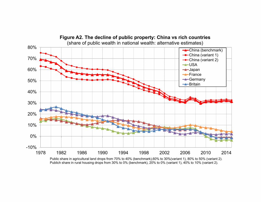
-10%

0%

10%

20%

30%

40%

50%

60%

70%

80%

1978 1982 1986 1990 1994 1998 2002 2006 2010 2014Public share in agricultural land drops from 70% to 40% (benchmark),60% to 30%(variant 1), 80% to 50% (variant 2). Publich share in rural housing drops from 30% to 0% (benchmark), 20% to 0% (variant 1), 40% to 10% (variant 2).

Figure A2. The decline of public property: China vs rich countries (share of public wealth in national wealth: alternative estimates)

China (benchmark)China (variant 1)China (variant 2)USAJapanFranceGermanyBritain

-10%

0%

10%

20%

30%

40%

50%

60%

70%

1978 1982 1986 1990 1994 1998 2002 2006 2010 2014

Figure A3. The decline of public property: China vs rich countries (share of public wealth in national wealth)

China USAJapan FranceBritain GermanyNorway

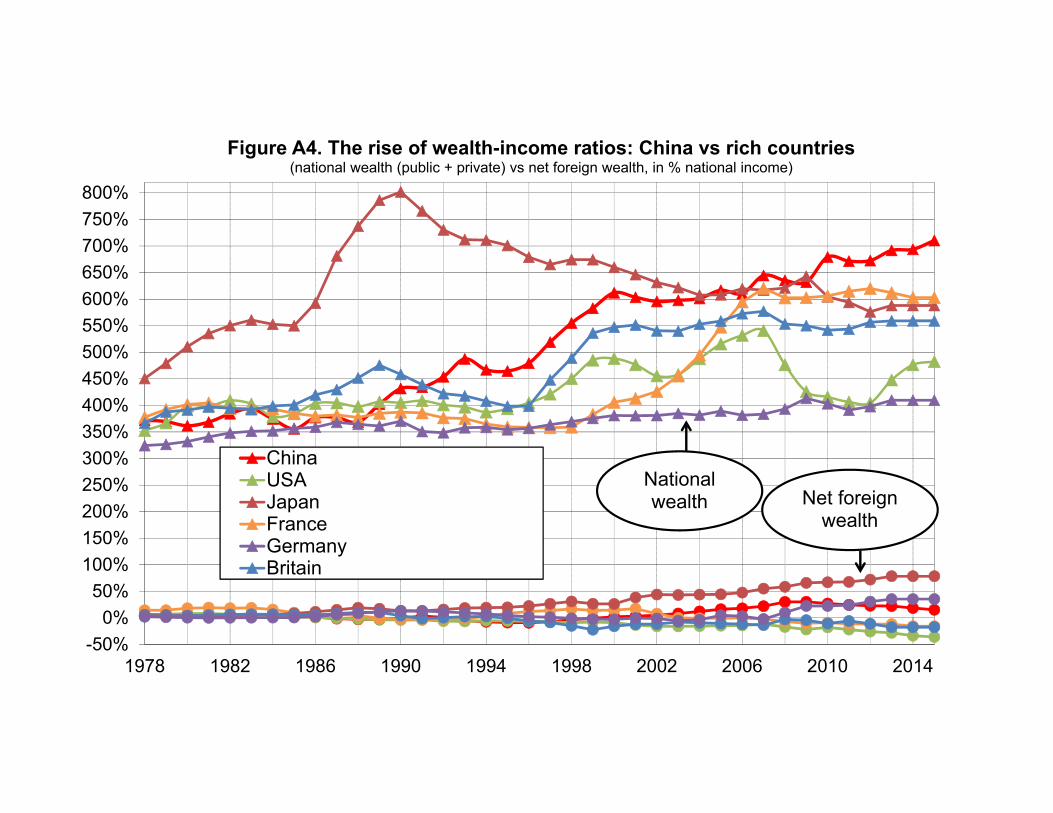
-50%0%

50%100%150%200%250%300%350%400%450%500%550%600%650%700%750%800%

1978 1982 1986 1990 1994 1998 2002 2006 2010 2014

Figure A4. The rise of wealth-income ratios: China vs rich countries (national wealth (public + private) vs net foreign wealth, in % national income)

ChinaUSAJapanFranceGermanyBritain

National wealth Net foreign

wealth

0

100

200

300

400

500

600

700

800

900

1,000

1,100

1,200

1,300

1,400

1978 1982 1986 1990 1994 1998 2002 2006 2010 2014

Figure A5. Population in urban and rural China, 1978-2015

Total populationTotal adult populationUrban adult populationRural adult population

100%

150%

200%

250%

300%

350%

400%

450%

500%

550%

600%

1978 1982 1986 1990 1994 1998 2002 2006 2010 2014

Figure A6. The rise of wealth-income ratios: China vs rich countries (private wealth (households), in % national income)

China

USA

France

Britain

-10%

0%

10%

20%

30%

40%

50%

60%

70%

1978 1982 1986 1990 1994 1998 2002 2006 2010 2014

Figure A7. The decline of public property: China vs rich countries (share of public wealth in national wealth)

China USA

Japan France

Britain Germany

40%

60%

80%

100%

120%

140%

160%

180%

200%

220%

240%

260%

280%

300%

1978 1982 1986 1990 1994 1998 2002 2006 2010 2014

Figure A8. The rise of financial intermediation: China vs rich countries (total domestic financial liabilities, in % domestic capital)

China

USA

Japan

France

Germany

0%

5%

10%

15%

20%

25%

30%

35%

1978 1982 1986 1990 1994 1998 2002 2006 2010 2014

Figure A9. The rise of foreign ownership: China vs rich countries (foreign financial liabilities, in % total domestic financial liabilities)

China

USA

Japan

France

Germany

β1996 β2015

Initial wealth effect

Cumulated new

savings

Capital gains

or losses

Initial wealth effect

Cumulated new savings

Capital gains or losses

Non-financial assets 163% 299% 31% 36% 231% 31% 36% 231%Net financial assets 85% 189% 16% 172% 1% 16% 144% 29%Non-financial assets 134% 74% 26% 28% 19% 26% 28% 19% Net financial assets 97% 149% 19% 63% 68% 19% 5% 126%

National Total 479% 710% 93% 298% 320% 93% 213% 405%

β1996 β2015

Initial wealth effect

Cumulated new

savings

incl. trade

balance

incl. net income

from property

incl. others(wage and current transfer)

Capital gains or losses

163% 251% 32% 56% 163%198% 342% 38% 218% 86%-9% 15% -2% 24% 37% -20% 6% -7%

120% 51% 23% 0% 28%3% 18% 1% 0% 18%

474% 677% 92% 298% 287%

Sources of national wealth accumulation in China, 1996-2015

Panel A: Sources of market-value national wealth accumulation

Sector Assets

Net wealth

Decomposition of wealth-national income ratio at time t+n

Method n°1: savings = private/public savings

Method n°2: savings = personal/government savings

Private

Public

Panel B: Sources of book-value national wealth accumulation

Assets

Net wealth Decomposition of wealth-national income ratio at time t+n

Notes:In Panel A Method n°1, private savings is equal to personal savings plus private share of retained earnings; public saving is equal to government saving plus public share of retained earnings. Source: PYZ2017NatoinalAccountsData, Sheet A49

Residential HouseOther domestic capital

Foreign wealthFarm lands

Reserved landsNational Wealth

10%

15%

20%

25%

30%

35%

40%

45%

50%

1978 1982 1986 1990 1994 1998 2002 2006 2010 2014

Figure B1a. Income inequality in China: corrected vs raw estimates

Top 10% (corrected)Top 10% (raw)Middle 40% (corrected)Middle 40% (raw)Bottom 50% (corrected)Bottom 50% (raw)

Distribution of pretax national income (before taxes and transfers, except pensions and unempl. insurance) among adults. Corrected estimates combine survey, fiscal, wealth and national accounts data. Raw estimates rely only on self-reported survey data.Equal-split-adults series (income of married couples divided by two). Pre-2006 series assume that the tax/survey upgrade factor is the same as the one observed on average over the 2006-2010 period when national-level tax data exist

2%3%4%5%6%7%8%9%

10%11%12%13%14%15%16%

1978 1982 1986 1990 1994 1998 2002 2006 2010 2014

B1b. Top 1% income share in China : corrected vs raw estimates

Top 1% (corrected pre-tax national income)

Top 1% (corrected fiscal income)

Top 1% (raw)

Distribution of pretax national income (before taxes and transfers, except pensions and unempl. insurance) among adults. Corrected estimates combine survey, fiscal, wealth and national accounts data. Raw estimates rely only on self-reported survey data.Equal-split-adults series (income of married couples divided by two). Pre-2006 series assume that the tax/survey upgrade factor is the same as the one observed on average over the 2006-2010 period when national-level tax data exist

4%5%6%7%8%9%

10%11%12%13%14%15%16%17%

1978 1982 1986 1990 1994 1998 2002 2006 2010 2014

Figure B2. Top 1% income share: urban vs rural China

ChinaUrban ChinaRural China

Distribution of pretax national income (before taxes and transfers, except pensions and unempl. insurance) among adults. Corrected estimates (combining survey, fiscal, wealth and national accounts data). Equal-split-adults series (income of married couples divided by two). Pre-2006 series assume that the tax/survey upgrade factor is the same as the one observed on average over the 2006-2010 period when national-level tax data exist

39%

40%

41%

42%

43%

44%

45%

46%

47%

48%

1978 1982 1986 1990 1994 1998 2002 2006 2010 2014

Figure B3. Middle 40% income share: urban vs rural China

ChinaUrban ChinaRural China

Distribution of pretax national income (before taxes and transfers, except pensions and unempl. insurance) among adults. Corrected estimates (combining survey, fiscal, wealth and national accounts data). Equal-split-adults series (income of married couples divided by two). Pre-2006 series assume that the tax/survey upgrade factor is the same as the one observed on average over the 2006-2010 period when national-level tax data exist

4%

6%

8%

10%

12%

14%

16%

18%

20%

22%

24%

26%

28%

1978 1982 1986 1990 1994 1998 2002 2006 2010 2014

Figure B4a. Bottom 50% vs Top 1% income share: China vs USA China: Bottom 50%China: Top 1%USA: Bottom 50%USA: Top 1%

Distribution of pretax national income (before taxes and transfers, except pensions and unempl. insurance) among adults. Corrected estimates (combining survey, fiscal, wealth and national accounts data). Equal-split-adults series (income of married couples divided by two).Pre-2006 series assume that the tax/survey upgrade factor is the same as the one observed on average over the 2006-2010 period when national-level tax data exist

4%

6%

8%

10%

12%

14%

16%

18%

20%

22%

24%

26%

28%

1978 1982 1986 1990 1994 1998 2002 2006 2010 2014

Figure B4b. Bottom 50% vs Top 1% income share: China vs France China: Bottom 50%China: Top 1%France: Bottom 50%France: Top 1%

Distribution of pretax national income (before taxes and transfers, except pensions and unempl. insurance) among adults. Corrected estimates (combining survey, fiscal, wealth and national accounts data). Equal-split-adults series (income of married couples divided by two). Pre-2006 series assume that the tax/survey upgrade factor is the same as the one observed on average over the 2006-2010 period when national-level tax data exist

22%

24%

26%

28%

30%

32%

34%

36%

38%

2006 2007 2008 2009 2010 2011 2012 2013 2014 2015

Figure B5a. Variants of top 10% income shares (Urban fiscal income)

Top 10% (survey data)

Top 10% (survey + tax data) (benchmarkestimates: uniform upgrade factors)Top 10% (survey + tax data) (2010 upgradefactors)Top 10% (survey+tax data) (yearly upgradefactors 2006-2010)Top 10% (survey + tax data) (2006 upgradefactors)

Distribution of pretax fiscal income (before all taxes and transfers, except pensions and unempl. insurance) among adults. Equal-split-adults series (income of married couples divided by two).

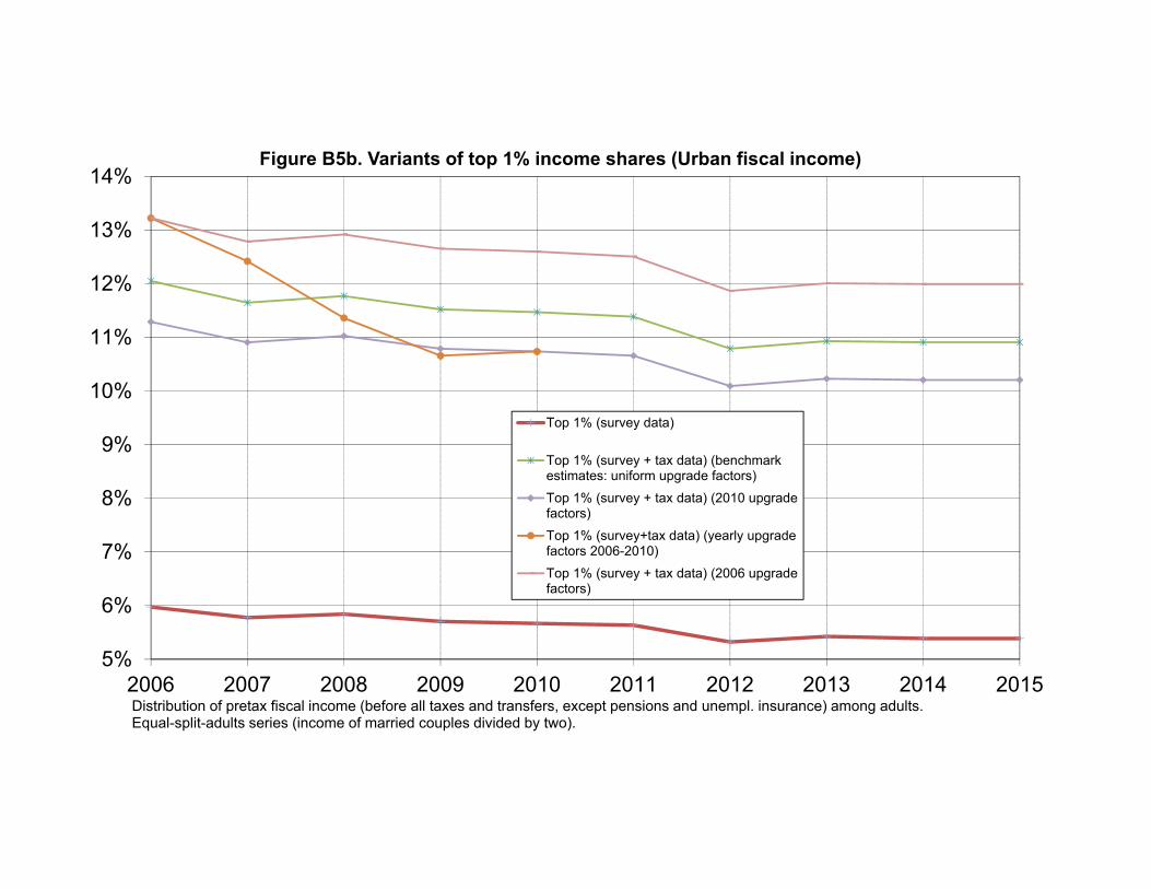
5%

6%

7%

8%

9%

10%

11%

12%

13%

14%

2006 2007 2008 2009 2010 2011 2012 2013 2014 2015

Figure B5b. Variants of top 1% income shares (Urban fiscal income)

Top 1% (survey data)

Top 1% (survey + tax data) (benchmarkestimates: uniform upgrade factors)Top 1% (survey + tax data) (2010 upgradefactors)Top 1% (survey+tax data) (yearly upgradefactors 2006-2010)Top 1% (survey + tax data) (2006 upgradefactors)

Distribution of pretax fiscal income (before all taxes and transfers, except pensions and unempl. insurance) among adults.Equal-split-adults series (income of married couples divided by two).

40%

41%

42%

43%

44%

45%

46%

47%

48%

2006 2007 2008 2009 2010 2011 2012 2013 2014 2015

Figure B5c. Variants of middle 40% income shares (Urban fiscal income)

Middle 40% (survey data)

Middle 40% (survey + tax data) (benchmarkestimates: uniform upgrade factors)Middle 40% (survey + tax data) ( 2010 upgradefactors)Middle 40% (survey+tax data) (yearly upgradefactors 2006-2010)Middle 40% (survey + tax data) ( 2006 upgradefactors)

Distribution of pretax fiscall income (before all taxes and transfers, except pensions and unempl. insurance) among adults.Equal-split-adults series (income of married couples divided by two).

21%

22%

23%

24%

25%

26%

27%

28%

29%

2006 2007 2008 2009 2010 2011 2012 2013 2014 2015

Figure B5d. Variants of Bottom 50% income shares (Urban fiscal income)

Bottom 50% (survey data)

Bottom 50% (survey + tax data) (benchmarkestimates: uniform upgrade factors)Bottom 50% (survey + tax data) (2010 upgradefactors)Bottom 50% (survey+tax data) (yearly upgradefactors 2006-2010)Bottom 50% (survey + tax data) (2006 upgradefactors)

Distribution of pretax fiscal income (before all taxes and transfers, except pensions and unempl. insurance) among adults.Equal-split-adults series (income of married couples divided by two).

18%

20%

22%

24%

26%

28%

30%

32%

34%

36%

38%

40%

42%

44%

1978 1982 1986 1990 1994 1998 2002 2006 2010 2014

Figure B6a. Variants of top 10% income shares (Rural fiscal income) Top 10% (survey data)

Top 10% (survey + tax data)(benchmark estimates:uniform upgrade factors)

Top 10% (survey + tax data) (estimates: 2006upgrade factors)

Top 10% (survey + tax data) (estimates: 2010upgrade factors)

Distribution of pretax fiscal income (before all taxes and transfers, except pensions and unempl. insurance) among adults.Equal-split-adults series (income of married couples divided by two).

3%4%5%6%7%8%9%

10%11%12%13%14%15%16%17%

1978 1982 1986 1990 1994 1998 2002 2006 2010 2014

Figure B6b. Variants of top 1% income shares (Rural fiscal income) Top 1% (survey data)

Top 1% (survey + tax data)(benchmark estimates:uniform upgrade factors)

Top 1% (survey + tax data) (estimates: 2006 upgradefactors)

Top 1% (survey + tax data) (estimates: 2010 upgradefactors)

Distribution of pretax fiscal income (before all taxes and transfers, except pensions and unempl. insurance) among adults.Equal-split-adults series (income of married couples divided by two).

38%

39%

40%

41%

42%

43%

44%

45%

46%

47%

48%

1978 1982 1986 1990 1994 1998 2002 2006 2010 2014

Figure B6c. Variants of Middle 40% income shares (Rural fiscal income)

Middle 40% (survey data)

Middle 40% (survey + tax data)(benchmarkestimates: uniform upgrade factors)

Middle 40% (survey + tax data) (estimates: 2006upgrade factors)

Middle 40% (survey + tax data) (estimates: 2010upgrade factors)

Distribution of pretax fiscal income (before all taxes and transfers, except pensions and unempl. insurance) among adults.Equal-split-adults series (income of married couples divided by two).

18%

20%

22%

24%

26%

28%

30%

32%

34%

1978 1982 1986 1990 1994 1998 2002 2006 2010 2014

Figure B6d. Variants of Bottom 50% income shares (Rural fiscal income)

Bottom 50% (survey data)

Bottom 50% (survey + tax data)(benchmarkestimates: uniform upgrade factors)

Bottom 50% (survey + tax data) (estimates: 2006upgrade factors)

Bottom 50% (survey + tax data) (estimates: 2010upgrade factors)

Distribution of pretax fiscal income (before all taxes and transfers, except pensions and unempl. insurance) among adults. Equal-split-adults series (income of married couples divided by two).

18%

20%

22%

24%

26%

28%

30%

32%

34%

36%

38%

40%

42%

44%

1978 1982 1986 1990 1994 1998 2002 2006 2010 2014

Figure B7a. Variants of top 10% income shares (China fiscal income) Top 10% (survey data)

Top 10% (survey + tax data)(benchmarkestimates: uniform upgrade factors)

Top 10% (survey + tax data) (estimates: 2006upgrade factors)

Top 10% (survey + tax data) (estimates: 2007upgrade factors)

Top 10% (survey + tax data) (estimates: 2008upgrade factors)

Top 10% (survey + tax data) (estimates: 2009upgrade factors)

Top 10% (survey + tax data) (estimates: 2010upgrade factors)

Distribution of pretax fiscal income (before all taxes and transfers, except pensions and unempl. insurance) among adults.Equal-split-adults series (income of married couples divided by two).

3%

4%

5%

6%

7%

8%

9%

10%

11%

12%

13%

14%

15%

16%

1978 1982 1986 1990 1994 1998 2002 2006 2010 2014

Figure B7b. Variants of top 1% income shares (China fiscal income) Top 1% (survey data)

Top 1% (survey + tax data)(benchmark estimates:uniform upgrade factors)

Top 1% (survey + tax data) (estimates: 2006 upgradefactors)

Top 1% (survey + tax data) (estimates: 2007 upgradefactors)

Top 1% (survey + tax data) (estimates: 2008 upgradefactors)

Top 1% (survey + tax data) (estimates: 2009 upgradefactors)

Top 1% (survey + tax data) (estimates: 2010 upgradefactors)

kkk

Distribution of pretax fiscal income (before all taxes and transfers, except pensions and unempl. insurance) among adults.Equal-split-adults series (income of married couples divided by two).

43%

44%

45%

46%

47%

48%

49%

50%

51%

52%

1978 1982 1986 1990 1994 1998 2002 2006 2010 2014

Figure B7c. Variants of Middle 40% income shares (China fiscal income) Middle 40% (survey data)

Middle 40% (survey + tax data)(benchmarkestimates: uniform upgrade factors)

Middle 40% (survey + tax data) (estimates: 2006upgrade factors)

Middle 40% (survey + tax data) (estimates: 2007upgrade factors)

Middle 40% (survey + tax data) (estimates: 2008upgrade factors)

Middle 40% (survey + tax data) (estimates: 2009upgrade factors)

Middle 40% (survey + tax data) (estimates: 2010upgrade factors)

Distribution of pretax fiscal income (before all taxes and transfers, except pensions and unempl. insurance) among adults.Equal-split-adults series (income of married couples divided by two).

14%

16%

18%

20%

22%

24%

26%

28%

30%

1978 1982 1986 1990 1994 1998 2002 2006 2010 2014

Figure B7d. Variants of Bottom 50% income shares (China fiscal income)

Bottom 50% (survey data)

Bottom 50% (survey + tax data)(benchmarkestimates: uniform upgrade factors)

Bottom 50% (survey + tax data) (estimates: 2006upgrade factors)

Bottom 50% (survey + tax data) (estimates: 2007upgrade factors)

Bottom 50% (survey + tax data) (estimates: 2008upgrade factors)

Bottom 50% (survey + tax data) (estimates: 2009upgrade factors)

Bottom 50% (survey + tax data) (estimates: 2010upgrade factors)

Distribution of pretax fiscal income (before all taxes and transfers, except pensions and unempl. insurance) among adults. Equal-split-adults series (income of married couples divided by two).

18%20%22%24%26%28%30%32%34%36%38%40%42%44%

1978 1982 1986 1990 1994 1998 2002 2006 2010 2014

Figure B8a. Variants of top 10% income shares (China national income) Top 10% (survey data)

Top 10% (survey + tax data)(benchmark estimates:uniform upgrade factors)

Top 10% (survey + tax data) (estimates: 2006upgrade factors)

Top 10% (survey + tax data) (estimates: 2007upgrade factors)

Top 10% (survey + tax data) (estimates: 2008upgrade factors)

Top 10% (survey + tax data) (estimates: 2009upgrade factors)

Top 10% (survey + tax data) (estimates: 2010upgrade factors)

Distribution of pretax national income (before all taxes and transfers, except pensions and unempl. insurance) among adults.Equal-split-adults series (income of married couples divided by two).

3%4%5%6%7%8%9%

10%11%12%13%14%15%16%17%

1978 1982 1986 1990 1994 1998 2002 2006 2010 2014

Figure B8b. Variants of top 1% income shares (China national income) Top 1% (survey data)

Top 1% (survey + tax data)(benchmark estimates:uniform upgrade factors)

Top 1% (survey + tax data) (estimates: 2006 upgradefactors)

Top 1% (survey + tax data) (estimates: 2007 upgradefactors)

Top 1% (survey + tax data) (estimates: 2008 upgradefactors)

Top 1% (survey + tax data) (estimates: 2009 upgradefactors)

Top 1% (survey + tax data) (estimates: 2010 upgradefactors)

kkk

Distribution of pretax national income (before all taxes and transfers, except pensions and unempl. insurance) among adults.Equal-split-adults series (income of married couples divided by two).

41%

42%

43%

44%

45%

46%

47%

48%

49%

50%

51%

52%

1978 1982 1986 1990 1994 1998 2002 2006 2010 2014

Figure B8c. Variants of Middle 40% income shares (China national income)

Middle 40% (survey data)

Middle 40% (survey + tax data)(benchmarkestimates: uniform upgrade factors)

Middle 40% (survey + tax data) (estimates: 2006upgrade factors)

Middle 40% (survey + tax data) (estimates: 2007upgrade factors)

Middle 40% (survey + tax data) (estimates: 2008upgrade factors)

Middle 40% (survey + tax data) (estimates: 2009upgrade factors)

Middle 40% (survey + tax data) (estimates: 2010upgrade factors)

Distribution of pretax national income (before all taxes and transfers, except pensions and unempl. insurance) among adults.Equal-split-adults series (income of married couples divided by two).

14%

16%

18%

20%

22%

24%

26%

28%

30%

1978 1982 1986 1990 1994 1998 2002 2006 2010 2014

Figure B8d. Variants of Bottom 50% income shares (China national income)

Bottom 50% (survey data)

Bottom 50% (survey + tax data)(benchmarkestimates: uniform upgrade factors)

Bottom 50% (survey + tax data) (estimates: 2006upgrade factors)

Bottom 50% (survey + tax data) (estimates: 2007upgrade factors)

Bottom 50% (survey + tax data) (estimates: 2008upgrade factors)

Bottom 50% (survey + tax data) (estimates: 2009upgrade factors)

Bottom 50% (survey + tax data) (estimates: 2010upgrade factors)

Distribution of pretax national income (before all taxes and transfers, except pensions and unempl. insurance) among adults. Equal-split-adults series (income of married couples divided by two).

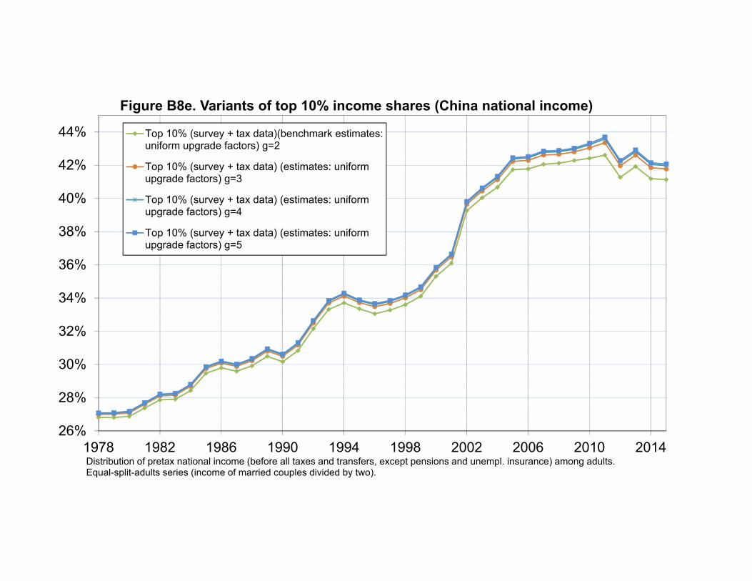
26%

28%

30%

32%

34%

36%

38%

40%

42%

44%

1978 1982 1986 1990 1994 1998 2002 2006 2010 2014

Figure B8e. Variants of top 10% income shares (China national income)

Top 10% (survey + tax data)(benchmark estimates:uniform upgrade factors) g=2

Top 10% (survey + tax data) (estimates: uniformupgrade factors) g=3

Top 10% (survey + tax data) (estimates: uniformupgrade factors) g=4

Top 10% (survey + tax data) (estimates: uniformupgrade factors) g=5

Distribution of pretax national income (before all taxes and transfers, except pensions and unempl. insurance) among adults.Equal-split-adults series (income of married couples divided by two).

3%4%5%6%7%8%9%

10%11%12%13%14%15%16%17%

1978 1982 1986 1990 1994 1998 2002 2006 2010 2014

Figure B8f. Variants of top 1% income shares (China national income)

Top 1% (survey + tax data)(benchmark estimates:uniform upgrade factors) g=2

Top 1% (survey + tax data) (estimates: uniformupgrade factors) g=5

Top 1% (survey + tax data) (estimates: uniformupgrade factors) g=4

Top 1% (survey + tax data) (estimates: uniformupgrade factors) g=3

Distribution of pretax national income (before all taxes and transfers, except pensions and unempl. insurance) among adults.Equal-split-adults series (income of married couples divided by two).

41%

42%

43%

44%

45%

46%

47%

48%

49%

50%

51%

52%

1978 1982 1986 1990 1994 1998 2002 2006 2010 2014

Figure B8g. Variants of Middle 40% income shares (China national income)

Middle 40% (survey + tax data)(benchmark estimates: uniformupgrade factors) g=2Middle 40% (survey + tax data) (estimates: uniform upgradefactors) g=3Middle 40% (survey + tax data) (estimates: uniform upgradefactors) g=4Middle 40% (survey + tax data) (estimates: uniform upgradefactors) g=5

Distribution of pretax national income (before all taxes and transfers, except pensions and unempl. insurance) among adults.Equal-split-adults series (income of married couples divided by two).

14%

16%

18%

20%

22%

24%

26%

28%

30%

1978 1982 1986 1990 1994 1998 2002 2006 2010 2014

Figure B8h. Variants of Bottom 50% income shares (China national income)

Bottom 50% (survey + tax data)(benchmarkestimates: uniform upgrade factors) g=2

Bottom 50% (survey + tax data) (estimates: uniformupgrade factors) g=4

Bottom 50% (survey + tax data) (estimates: uniformupgrade factors) g=5

Bottom 50% (survey + tax data) (estimates: uniformupgrade factors) g=3

Distribution of pretax national income (before all taxes and transfers, except pensions and unempl. insurance) among adults. Equal-split-adults series (income of married couples divided by two).

0.9

1.0

1.1

1.2

1.3

1.4

1.5

1.6

1.7

80 81 82 83 84 85 86 87 88 89 90 91 92 93 94 95 96 97 98 99 99.199.299.399.499.5

Figure B9a. Upgrade Factors for Income Threshold

2006

2007

2008

2009

2010

2011

2012

2013

2014

2015

Based on provincal tax data2011-2015

Based on national tax data

2006-2010

0.9

1.2

1.5

1.8

2.1

2.4

2.7

3.0

3.3

80 81 82 83 84 85 86 87 88 89 90 91 92 93 94 95 96 97 98 99 99.199.299.399.499.5

Figure B9b. Upgrade Factors for Interm. Income

2006

2007

2008

2009

2010

2011

2012

2013

2014

2015

Based on provincal tax data

2006-2010

Based on national tax data

2011-2015

0.0%

0.2%

0.4%

0.6%

0.8%

1.0%

1.2%

1.4%

1.6%

1.8%

2.0%

1982

1984

1986

1988

1990

1992

1994

1996

1998

2000

2002

2004

2006

2008

2010

2012

2014Figure B10a. Total Income Tax as a Fraction of National Income of China

Income tax revenue

Imputed total income tax (unif)

Imputed total income tax(2010corr)Imputed total income tax(survey)

0.0%

0.2%

0.4%

0.6%

0.8%

1.0%

1.2%

1982

1984

1986

1988

1990

1992

1994

1996

1998

2000

2002

2004

2006

2008

2010

2012

2014Figure B10b. Income Tax on Wage as a Fraction of National Income of China

Income tax on wage

Imputed income tax on wage(unif)Imputed income tax on wage(2010corr)Imputed income tax on wage(survey)

0.0%

0.2%

0.4%

0.6%

0.8%

1.0%

1982

1984

1986

1988

1990

1992

1994

1996

1998

2000

2002

2004

2006

2008

2010

2012

2014Figure B10c. Non-wage Income Tax as a Fraction of National Income of China

Non-wage income tax revenue

Imputed non-wage income tax(unif)Imputed non-wage income tax(2010corr)Imputed non-wage income tax(survey)

28%

30%

32%

34%

36%

38%

40%

42%

44%

46%

48%

50%

1978 1982 1986 1990 1994 1998 2002 2006 2010 2014

Figure B11b Income share of bottom 50% in bottom 80% income group in rural China

Fiscal Income (PYZ2017 corrected)

Survey Income (CHIP raw)

We corrected the estimation of CHIP with weight variable suggested by Li Shi (2013) in 2002. In year 2012, CHIP only report household disposable income, for urban resident, this is equal to aftet-tax-after-transfer income. NBS tabulation uses the concept of total income, which is before-tax-after-transfer income. NBS TP Average Adult Income = income per capita/adult ratio, income per capita is reported by NBS, we use national adult ratio for both rural and urban China. Equal-split-adults series (income of married couples divided by two). Corrected estimates (combining survey, fiscal, wealth and national accounts data).

32%

34%

36%

38%

40%

42%

44%

46%

48%

50%

52%

54%

56%

1978 1982 1986 1990 1994 1998 2002 2006 2010 2014

Figure B11b Income share of bottom 50% in bottom 80% income group in urban China

Fiscal Income (PYZ2017 corrected)

Survey Income (CHIP raw)

We corrected the estimation of CHIP with weight variable suggested by Li Shi (2013) in 2002. In year 2012, CHIP only report household disposable income, for urban resident, this is equal to aftet-tax-after-transfer income. NBS tabulation uses the concept of total income, which is before-tax-after-transfer income. NBS TP Average Adult Income = income per capita/adult ratio, income per capita is reported by NBS, we use national adult ratio for both rural and urban China. Equal-split-adults series (income of married couples divided by two). Corrected estimates (combining survey, fiscal, wealth and national accounts data).

5%

7%

9%

11%

13%

15%

17%

19%

21%

23%

25%

1978 1982 1986 1990 1994 1998 2002 2006 2010 2014

Figure B11c Income share of bottom 25% in bottom 80% income group in rural China

Fiscal Income (PYZ2017 corrected)

Survey Income (CHIP raw)

We corrected the estimation of CHIP with weight variable suggested by Li Shi (2013) in 2002. In year 2012, CHIP only report household disposable income, for urban resident, this is equal to aftet-tax-after-transfer income. NBS tabulation uses the concept of total income, which is before-tax-after-transfer income. NBS TP Average Adult Income = income per capita/adult ratio, income per capita is reported by NBS, we use national adult ratio for both rural and urban China. Equal-split-adults series (income of married couples divided by two). Corrected estimates (combining survey, fiscal, wealth and national accounts data).

5%

7%

9%

11%

13%

15%

17%

19%

21%

23%

25%

1978 1982 1986 1990 1994 1998 2002 2006 2010 2014

Figure b11d Income share of bottom 25% in bottom 80% income group in urban China

Fiscal Income (PYZ2017 corrected)

Survey Income (CHIP raw)

We corrected the estimation of CHIP with weight variable suggested by Li Shi (2013) in 2002. In year 2012, CHIP only report household disposable income, for urban resident, this is equal to aftet-tax-after-transfer income. NBS tabulation uses the concept of total income, which is before-tax-after-transfer income. NBS TP Average Adult Income = income per capita/adult ratio, income per capita is reported by NBS, we use national adult ratio for both rural and urban China. Equal-split-adults series (income of married couples divided by two). Corrected estimates (combining survey, fiscal, wealth and national accounts data).

23%

25%

27%

29%

31%

33%

1978 1982 1986 1990 1994 1998 2002 2006 2010 2014

Figure B11e Income share of 2nd quartile in bottom 80% income group in rural China

Fiscal Income (PYZ2017 corrected)

Survey Income (CHIP raw)

We corrected the estimation of CHIP with weight variable suggested by Li Shi (2013) in 2002. In year 2012, CHIP only report household disposable income, for urban resident, this is equal to aftet-tax-after-transfer income. NBS tabulation uses the concept of total income, which is before-tax-after-transfer income. NBS TP Average Adult Income = income per capita/adult ratio, income per capita is reported by NBS, we use national adult ratio for both rural and urban China. Equal-split-adults series (income of married couples divided by two). Corrected estimates (combining survey, fiscal, wealth and national accounts data).

23%

25%

27%

29%

31%

33%

1978 1982 1986 1990 1994 1998 2002 2006 2010 2014

Figure B11f Income share of 2nd quartile in bottom 80% income group in urban China

Fiscal Income (PYZ2017 corrected)

Survey Income (CHIP raw)

We corrected the estimation of CHIP with weight variable suggested by Li Shi (2013) in 2002. In year 2012, CHIP only report household disposable income, for urban resident, this is equal to aftet-tax-after-transfer income. NBS tabulation uses the concept of total income, which is before-tax-after-transfer income. NBS TP Average Adult Income = income per capita/adult ratio, income per capita is reported by NBS, we use national adult ratio for both rural and urban China. Equal-split-adults series (income of married couples divided by two). Corrected estimates (combining survey, fiscal, wealth and national accounts data).

47%

49%

51%

53%

55%

57%

59%

61%

63%

65%

67%

69%

71%

1978 1982 1986 1990 1994 1998 2002 2006 2010 2014

Figure B11g Income share of top 30% in bottom 80% income group in rural China

Fiscal Income (PYZ2017 corrected)

Survey Income (CHIP raw)

We corrected the estimation of CHIP with weight variable suggested by Li Shi (2013) in 2002. In year 2012, CHIP only report household disposable income, for urban resident, this is equal to aftet-tax-after-transfer income. NBS tabulation uses the concept of total income, which is before-tax-after-transfer income. NBS TP Average Adult Income = income per capita/adult ratio, income per capita is reported by NBS, we use national adult ratio for both rural and urban China. Equal-split-adults series (income of married couples divided by two). Corrected estimates (combining survey, fiscal, wealth and national accounts data).

44%

46%

48%

50%

52%

54%

56%

58%

60%

62%

64%

66%

68%

1978 1982 1986 1990 1994 1998 2002 2006 2010 2014

Figure B11h Income share of top30% in bottom 80% income group in urban China

Fiscal Income (PYZ2017 corrected)

Survey Income (CHIP raw)

We corrected the estimation of CHIP with weight variable suggested by Li Shi (2013) in 2002. In year 2012, CHIP only report household disposable income, for urban resident, this is equal to aftet-tax-after-transfer income. NBS tabulation uses the concept of total income, which is before-tax-after-transfer income. NBS TP Average Adult Income = income per capita/adult ratio, income per capita is reported by NBS, we use national adult ratio for both rural and urban China. Equal-split-adults series (income of married couples divided by two). Corrected estimates (combining survey, fiscal, wealth and national accounts data).

5%9%

13%17%21%25%29%33%37%41%45%49%53%57%

1 1.1 1.2 1.3 1.4 1.5 1.6 1.7 1.8 1.9 2

Figure B12a Wealth shares: variants for different upgrade factors (2002)

Top 10% Wealth ShareTop 1% Wealth ShareMiddle 40% Wealth ShareBottom 50% Wealth Share

When upgrade factor is greater than 2, average survey wealth per adult is greater than average wealth per adult based on national accounts. Thus the upgrade factor has to be smaller than 2. Raw wealth tabulation cut at p=0.90

Bench Mark

5%9%

13%17%21%25%29%33%37%41%45%49%53%57%61%65%69%73%77%

1 1.1 1.2 1.3 1.4 1.5 1.6 1.7 1.8 1.9 2

Figure B12b Wealth shares: variants for different upgrade factors (2012)

Top 10% Wealth ShareTop 1% Wealth ShareMiddle 40% Wealth ShareBottom 50% Wealth Share

When upgrade factor is greater than 2, average survey wealth per adult is greater than average wealth per adult based on national accounts. Thus the upgrade factor has to be smaller than 2. Raw wealth tabulation cut at p=0.90

Bench Mark

Table S2 Comparison Among Different Data SetsIncome share

SurveyIncomeSource

NBS TB CHIP CHIP/NBS TB NBS TB CHIP CHIP/N

BS TB NBS TB CHIP CHIP/NBS TB NBS TB CHIP CHIP/N

BS TB

CorrectedFiscal

Income(PYZ201

7)

CHIP CHIP/PYZ2017

CorrectedFiscal

Income(PYZ201

7)

CHIP CHIP/PYZ2017

CorrectedFiscal

Income(PYZ201

7)

CHIP CHIP/PYZ2017

Year1988 38% 35% 94% 45% 45% 99% 17% 20% 117% 2.7% 4.0% 146% 23% 22% 94% 31% 31% 100% 46% 47% 102%1995 35% 32% 89% 46% 46% 101% 19% 22% 119% 3.2% 4.1% 129% 22% 19% 89% 31% 30% 99% 48% 50% 106%1999 33% 29% 88% 47% 48% 103% 20% 23% 114% 3.6% 4.0% 114% 21% 17% 85% 30% 30% 98% 49% 53% 107%2002 28% 25% 90% 47% 48% 102% 24% 26% 107% 5.3% 5.3% 100% 17% 14% 79% 30% 30% 102% 53% 56% 106%2012 29% 27% 93% 47% 47% 100% 24% 26% 108% 5.2% 5.4% 104% 18% 16% 90% 30% 30% 100% 53% 54% 103%

1988 30% 26% 89% 47% 48% 102% 24% 26% 110% 4.2% 5.1% 122% 19% 16% 84% 30% 29% 99% 52% 55% 106%1995 27% 24% 91% 47% 46% 98% 26% 30% 112% 5.1% 7.2% 142% 17% 16% 92% 29% 29% 99% 54% 56% 103%2002 25% 26% 104% 47% 47% 101% 29% 27% 95% 6.3% 5.6% 88% 16% 16% 104% 29% 29% 100% 56% 55% 99%2012 23% 24% 101% 47% 48% 102% 30% 28% 95% 7.1% 6.3% 89% 14% 14% 99% 29% 29% 99% 57% 57% 101%

Notes:we corrected the estimation of CHIP with weight variable suggested by Li Shi (2013) in 2002.In year 2012, CHIP only report household disposable income, for urban resident, this is equal to aftet-tax-after-transfer income. NBS tabulation uses the concept of total income, which is before-tax-after-transfer income.NBS TP Average Adult Income = income per capita/adult ratio, income per capita is reported by NBS, we use national adult ratio for both rural and urban China.Equal-split-adults series (income of married couples divided by two).Corrected estimates (combining survey, fiscal, and national accounts data).

bottom 50% middle 40% top 10% top 1%

Urban China

Rural China

bottom 25% in bottom 80% middle 25% in bottom 80% top 30% in bottom 80%

Urban China

Rural China