capital structure and income inequality - …summit.sfu.ca/system/files/iritems1/14646/saikat...
TRANSCRIPT
CAPITAL STRUCTURE AND INCOMEINEQUALITY
by
Saikat Sarkar
PhD in Economics, University Of Tampere and 2008
PROJECT SUBMITTED IN PARTIAL FULFILLMENT OF
THE REQUIREMENTS FOR THE DEGREE OF
MASTER OF SCIENCE IN FINANCE
In the Master of Science in Finance Program
of the
Faculty
of
Business Administration
c Saikat Sarkar 2014
SIMON FRASER UNIVERSITY
Term Fall 2014
All rights reserved. However, in accordance with the Copyright Act of Canada,
this work may be reproduced, without authorization, under the conditions for
Fair Dealing. Therefore, limited reproduction of this work for the purposes of
private study, research, criticism, review and news reporting is likely to be in
accordance with the law, particularly if cited appropriately.

Approval
Name: Saikat Sarkar
Degree: Master of Science in Finance
Title of Project: Capital Structure and Income Inequality
Supervisory Committee:
___________________________
Associate Professor and Amir Rubin
Senior Supervisor
Correct Title �Associate Professor
___________________________
Professor and George Blazenko
Second Reader
Correct Title �Professor
Date Approved: ___________________________
ii

Abstract
Using the new issuance of equity and corporate bond data series, this
research �nds that recent surge in top incomes shares have negative e¤ect
on the capital structure choice of North American �rms. This paper also
uses information from �rm speci�c and macroeconomic variables to explain
the dynamics of capital structure choice of OECD �rms. The result of
this empirical study provides some of the insights from modern capital
structure theory. But these traditional determinants might not have the
robust explanatory power in explaining the capital structure choice of a
�rm.
Key words: Capital structure, Top inocme shares, Macroeconomic fac-
tors, Firm speci�c factors
iii

Acknowledgements
The completion of this work represents an important turning-point,
which could not have been achieved without the help of my colleagues,
friends and family. There are several people I need to thank for their
valuable supports.
First of all, I would like to express the earnest gratitude to my supervi-
sor, Prof. Amir Rubin, who has the attitude and the substance of a genius:
he continually and convincingly conveyed a spirit of adventure in regard to
research, and an excitement in regard to teaching. I am grateful to him.
His unconditional commitment and con�dence in the success of this project
was an invaluable source of motivation. I also wish to thank the another
supervisor of this project, Prof. George Blazenko, for accurate comments
and valuable ideas for further development. I could not come this far with-
out the original ideas and support from Prof. Amir Rubin. Without his
guidance and persistent help this project would not have been possible. I
am also indebted to Prof. Andrey Pavlov, Prof. Peter Klein, Prof. Avi
Bick, Prof. Anton Theunissen for their help, suggestions, guidance and
inspiration during the entire program.
In addition, I would like to thank Shuhash Shimon and Mark Bodnar
for their excellent guidance in collecting data for this project. Moreover,
the discussions with the seminar participants in the Faculty of Business
Administration, Simon Fraser University, Canada have been very helpful.
Finally, I would like to express my deepest gratitude to those closest to
me: my parents, my lovely wife, my brother and sisters and to my brother
in law Dr Pronab Das.
iv

Table of Contents
Approval ii
Abstract iii
Acknowledgements vi
Table of Contents v
List of Tables vi
Introduction 1
Model 4
Data 7
Explaining the capital structure 14
Some robustness analysis of the results 25
Conclusions 30
v

List of Tables
Table Number Page number
Table-1 9
Table-2 10
Table-3 12
Table-4 13
Table-5 15
Table-6 18
Table-7 20
Table-8 26
Table-9 28
vi

1 Introduction
The increasing share of the top income earners in total income in the United
States, and Canada (see Atkinson, 2007; Piketty and Saez, 2007) has been
one of the most hotly discussed topics over the last few years. Piketty and
Saez (2007) argued that top capital shares in Anglo Saxon countries were
mostly induced by capital gain, although the surge in top income shares
is not common in non-English speaking countries (particularly in France,
Japan and Switzerland). Accumulated income stimulates the top income
earners to buy more risky assets over less risky assets. Over time investors
increase their average equity ownership. However, the empirical insights
into how recent surge in top incomes shares in many advanced countries
a¤ect the capital structure choice of a �rm is still missing. This research
provides novel facts and shows that top income shares have negative e¤ect
on the capital structure choice of a �rm.
Top income shares are computed by dividing the observed top income
by the equivalent total income earned by the entire (tax) population, had
everyone �lled a personal tax return. Capital structure refers to the way
a corporation �nances its assets through some combination of equity and
debt. According to Modigliani and Miller (1958) in a perfect capital mar-
ket, i.e. in a world without tax, the concept of capital structure is not
relevant in �nancing for a project. Certainly in this framework institu-
tional and macroeconomic factors (e.g., economic growth rate, top income
shares, in�ation etc.) do not a¤ect the capital structure choice of a �rm.
But imperfections exist in the real world and Modigliani and Miller�s model
falls behind to capture these realities. However, theories like the Trade-o¤
1

model, the Pecking Order hypothesis, the Agency Theoretic framework and
the Market Timing theory address some of the issues of imperfections of
real world.
Trade-o¤ model is based on target capital structure and allows tax
shield as a bene�t and bankruptcy as a cost of debt. The theory states
that it is a trade-o¤ between costs and bene�ts of debt that can establish a
target level of debt for a �rm. In the Pecking Order theory, �rms prefer to
�nance their activities using retained earnings to minimize the asymmetric
information between insiders within a �rm and capital markets. If retained
earnings are inadequate, they turn to the use of debt. Equity �nancing is
only used as a last resort.
In the Agency Theoretic framework, potential con�ict of interest be-
tween inside and outside investors determines the target capital structure
of a �rm. Here, agency cost might evolve either in a circumstances of asset
substitution (i.e., replace equity by accruing more debt while investing) or
underinvestment. Underinvestment in the sense that high debt oriented
�rm might lose the opportunity of some attractive investment opportunity
due to the debt overhang problem (Jensen and Meckling (1976), Myers
(1977)). In this setting, the debt holders have the ability to extract some
of the net present value. Thus, management has an incentive to reject posi-
tive NPV (net present value) projects, even though they have the potential
to increase �rm value. Lastly Market Timing hypothesis assumes that there
are changes in market-to-book values which will create permanent changes
on �rm�s capital structure. It contradicts the idea of Trade-o¤ theory. In
this Market Timing hypothesis, �rms try to time the market by using debt
when it is cheap and equity when it seems cheap.
2

Obviously, there is close links between these theories discussed above
and it is very di¢ cult to distinguish the hypothesis of capital structure
theory particularly in an empirical framework. Potential variables that
describe the Trade-o¤ theory could also be used as important variables for
other capital structure theories and vice versa. As a result, recent empirical
research has focused on capital structure by using variety of variables that
can be justi�ed by any or all of the models.
Most of the empirical evidence on capital structure theory are based
on studies of the determinants of corporate debt ratios (see Titman and
Wessel (1988), Rajan and Zingales (1995)) and studies of �nancing choice
(i.e., choice between issuing �rm�s debt versus equity) (Booth, Ivazian,
Demirguc-Kunt andMaksimovic (2001), Banjeree, Heshmati, andWhilborg
(2004), Frank and Goyal (2009), Jong, Kabir and Nguyen (2008) among
others). These empirical studies show that the �rm-speci�c factors (e. g.,
�rm size, tangibility, intangibility, liquidity, market risk, research and de-
velopment, pro�tability, uniqueness and corporate tax rate) are important
in determining the capital structure of a �rm.
Another stream of research explains the capital structure choice based
on institutional and macroeconomic factors. Booth, Ivazian, Demirguc-
Kunt and Maksimovic (2001) and Frank and Goyal (2004), Jong, Kabir
and Nguyen (2008) documented the importance of domestic macroeconomic
factors in the empirical research of capital structure theory. They report
that macroeconomic factors (e.g., market rate return, market risk, economic
growth rate, in�ation rate, �nancial development and Millers tax term)
seem to have explanatory power to determine the capital structure choice
of a �rm.
3

Recently, Kacperczyk, Nosal and Stevens (2014) build a noise rational
expectations equilibrium model on the basis of information based frame-
work. In their model, they assumed that sophisticated investors have capac-
ity to access superior information over non-sophisticated investors. They
have ability to invest in better assets and generate pro�t through trading.
Consequently, sophisticated investors accumulate more wealth over time
and the investment of accumulate wealth in turn earn even more pro�t.
Eventually sophisticated investors allocate more of their resources on risky
assets than less risky assets and increase their average equity ownership.
However, the detailed empirical treatments of similar thought are still
missing particularly for the recent years. This research provides new empir-
ical evidence based on �rm�s new corporate bond and new equity issuance
data and shows that top income shares has negative e¤ect on the capital
structure choice of a �rm. That means that in presence of high top income
inequality, rich people tend to buy more stocks than bonds and �rms would
tend to issue more equity as opposed to debt. Hence investors increase their
average equity ownership relative to debt.
The rest of the paper proceeds as follows. In Section 2, a leverage model
of capital structure is speci�ed introducing the econometric analysis and
explaining the determinants of the capital structure. Section 3 presents the
data analysis. Section 4 contains the empirical results, Robustness analysis
is reported in Section 5 and section 6 concludes.
2 Model
As mentioned before, it is very di¢ cult to distinguish the hypothesis of
capital structure theory, discussed in the introductory part, particularly
4

in an empirical framework. Empirical research mostly focused on leverage
ratio by using variety of variables that can be justi�ed by any or all of the
models capital structure. Previous empirical evidence shows that capital
structure choice of a �rm not only depends upon the �rm-speci�c factors
but also on the country�s institutional factors and macroeconomic condi-
tions (Booth et.al (2001), Jong, Kabir and Nguyen (2008); Frank and Goyal
(2004)). We explore the e¤ect of top income shares on �rms�capital struc-
ture choice while controlling the e¤ect of macroeconomic and �rm-speci�c
variables.
In the process of developing the econometric model we assume that the
observed leverage ratio of �rm i at time t, denoted as yit. The expected
leverage ratio can be explain by
E (yit) = �1Topit + �2X=it + �t+ ui; (1)
where, the term Topit represents the top income shares of the rich, Xit
is the vector of control variables that we are interested in as well. The
terms ui and �t represent �xed country and time e¤ect respectively.
Let the error between actual and expected
"it = yit � E (yit) (2)
If the leverage ratio, represented by yit is auto-correlated then estimated
residuals fail to follow the assumptions underlying the OLS method. To
capture the possible autocorrelation that may exist in the leverage ratio
series, we assume
"it = �yit�1 + �it (3)
5

Combining equations with (1), (2) and (3) yields a general equation for
a leverage ratio
yit = 1yit�1 + 2Topit + 3X=it + �t+ ui + �it (4)
The variable Xit includes macroeconomic and �rm speci�c factors (e.g.,
�rm size, tangibility, intangibility, pro�tability, sales, liquidity, market risk,
top income shares, in�ation rate, and economic growth rate, rate of market
return, �nancial system and Miller tax term). The above dynamic panel
model could be estimated by OLS method but the assumptions underly-
ing the standard �xed e¤ects model are likely to be violated. Besides the
inclusion of the lagged dependent variable is problematic since it is cor-
related with the unobserved �xed e¤ects. Thereby, we could get biased
estimates. This bias is reduced when the actual time horizon T is large
(Nickell, 1981). We therefore apply the �rst di¤erence estimator which
relies on the assumption that the �rst di¤erences of the error terms are
serially uncorrelated. The �rst di¤erence panel model is as follows
yit = 1 (yit�1 � yit�2) + 2 (Topit � Topit�1) + (5)
3
�X=it �X
=it�1
�+ � (t� t+ 1) + �it � �it�1
(yit � yit�1) = 1 (yit�1 � yit�2)+ 2 (Topit � Topit�1) (6)
+ 3
�X=it �X
=it�1
�+� (t� t+ 1)+ (�it��it�1)
�yit = 0 + 1�yit�1 + 2�Topit + 3�X=it + vit; (7)
6

where 0 = � and vit = (�it��it�1)
The parameter 2 < 0 implies that top income shares has negative e¤ect
on the leverage ratio of a �rm which means: during time of high top income
inequality, rich people prefer to buy more risky assets than less risky assets.
The nice feature of the model represented by equation (3) is to capture the
possible auto correlation that arises in the leverage ratio term. We could
apply OLS method to estimate this model, provided that the error term
vit is normally distributed. Generally, GMM (Generalized method of mo-
ments) might be an appropriate procedure to estimate the dynamic panel
model. However, Flannery and Hankins (2013) documented that standard
error corrected LSDV (Least Squares Dummy Variable) also performs well
in estimating dynamic �xed e¤ect than panel regression model regardless
of the quality and size of the data (see also Judson and Owen (1999), Du�o
and Mullainathan (2004) and Atkinson and Leigh (2010)). Therefore, we
also apply the LSDV (Least Squares Dummy Variable) regression to esti-
mate the equation (3). For the purpose of robustness, we also re-estimate
the model represented by equation (3) while allowing �xed time e¤ects
and/or unobserved country-speci�c trends in the estimation process.
3 Data
This study is based on the top income shares, IPO (Initial public o¤ering)
and Corporate Bond issuance data. The top income shares data is available
for a long period of time for all the advanced countries in Top Income Shares
database. Statistical analysis, based on long and quality data series is
always elegant. But, the unavailability of macroeconomic and �rm speci�c
variables restricts our sample for the period of 1995 to 2013.
7

Our new equity issues (i.e., IPO issuance) and new debt issues (i.e.,
corporate bond issuance data) for OECD countries are collected from the
Thomson-Reuters Deal Database. We exclude utility companies (SIC codes
4900 �4999), and �nancial �rms (SIC codes 6000 �6999) from our sample.
We also impose some restrictions to our sample. IPO issuing �rms must be
listed in the stock exchange. IPO proceeds must be positive and exclude
depositary receipts, income shares, capital shares, partnerships, unit o¤ers,
closed-end funds, sub voting shares, options, while collecting the IPO issues
data1.
Similarly we exclude utility companies (SIC codes 4900 �4999), and
�nancial �rms (SIC codes 6000 �6999) while collecting the corporate bond
issuance data. We also restrict our sample to �xed rate bond that are
not matured within one year, and non-callable, non-puttable, non-sinking
funds, non-convertible and non-mortgage bonds. We further restrict our
sample based on Standard and Poor�s and Moody�s credit ratings. We
exclude all corporate bonds whose average credit rating is lower than B.
We use Top Income Shares database for top income shares data. Macro-
economic variables are collected from Financial Development of Beck,Thorsten,
Asli Demirgüç-Kunt and Ross Levine (2012) and OECD database. Firm-
speci�c variables are collected from COMPUSTAT and the COMPUSTAT
Global database. Tables-1 Table-2 and Table-3 de�ne the variables used in
this research and report their sources in details.
Following Baker and Wurgler (2002), we de�ne the leverage of �rm as
1The whole sample has only four REITs (Real estate investment trust) class of IPOissues and REITs are not excluded from our sample. We do not impose restriction onIPOs with an o¤er price of at least $5.00 and also relax the restriction on the listing inmajor stock exchanges. Later in the robustness section we allow all these restrictionsto our sample while computing IPO proceeds and re-assess the whole analysis for theNorth American region.
8

Table 1Description of macroeconomic factors
Variables Variable de�nation Source
Top1 Share of total income earned by The world top incomeincomes (P99-P100). database
Top1/9 Income share of top 1%(P99-P100) The world top incomedevided by income share earned databaseby the rest of the top 9%(P90-P99).
IvP(�) The Inverted Pareto-Lorenge coe¢ cient The world top incomeis a measure of the concentartion databaseof wealth among the rich.
In�ation Rate In�ation: Rate of change in the World bankconsumer price index.
GDPpc Natural logarithm of gross domestic World bankproduct per capita.
Personal Tax (Ti) Top marginal tax: Statutory tax rate. OECD database
Dividend Tax (Te) Personal dividend tax rate. OECD database
Corporate Tax (Tc) Combined Corporate income tax rate. OECD database
Rate of Return Yearly stock maket return index. Kenneth R. French- data library
Stock Market Stock market capitalisation: Value Financial developmentDevplopment of listed shares to GDP. and structure database
Bond Market Domestic debt securities issued Financial developmentDevplopment by Govt. and �nancial institutions and and structure database
corporations as a share of GDP.
Financial Ratio of Bond Market Development Levine (2002)System to Stock Market Development
Miller Tax Term 1�(1� Tc) (1� Te)(1� Ti)
Booth et al (2001)
9

Table 2Description of �rm speci�c �nancial factors
Variables Variable de�nation Source
Size Size is de�ned as the natural COMPUSTAT andlogarithm of total assets (AT). COMPUSTAT global
Tang Tangibility is de�ned as the ratio of COMPUSTAT andnet property, plant, and equipment COMPUSTAT global(PPENT) to total assets (AT).
Intang Intangibility is de�ned as the ratio of COMPUSTAT andintangibles (INTAN) to assets (AT). COMPUSTAT global
Pro�tability Pro�titability is de�ned as the ratio of COMPUSTAT andoperating income before depreciation COMPUSTAT global(OIBDP) to total assets (AT).
Sales The natural logarithm of sales (SALE). COMPUSTAT andCOMPUSTAT global
Liquidity Liquidity is de�ned as the ratio of current COMPUSTAT andasset (ACT) to current liability (LCT). COMPUSTAT global
Market Risk Market risk is measured by the standard Kenneth R. Frenchdeviation of stock market returns. - data library
10

the ratio of proceeds amount raised from the new debt issues over the sum
of the proceeds amount collected from both new issues of debt and equity.
A �rm is de�ned as issuing new equities when it raises fund through IPO
issuance. Similarly, a �rm is de�ned as issuing new debt when it raises
capital through corporate bond issuance from the public market. The key
disadvantage of this approach is that it ignores the source of private �nanc-
ing and private debt which seems to be much more common in corporate
world. The data series are gross yearly total of IPO issues and corporate
debt issues that do not subtract out repurchases or debt retirements.
Our main depended and independent variables are leverage ratio of a
�rm and top income shares respectively. All the other independent variables
used in this study and their measurement are largely adopted from existing
literature. The macro economic variables, which will be treated as control
variables in the econometric analysis, are: gross domestic product, in�ation
rate, corporate tax, personal tax, dividend tax, and stock market rate of
return, market risk, �nancial system, and Miller�s tax term.
Another set of dependent variables, treated as control variables in the
econometric analysis, is the �rm-speci�c factors. The �rm speci�c-factors
are: �rm size, tangibility, intangibility, pro�tability, sales, and liquidity.
These variables needed be obtained from the balance sheet of issuing �rms
for the purpose of this analysis. In order to collect that �nancial infor-
mation we �rst use Thomson-Reuters Deal Database. Unfortunately, �rm-
speci�c factors of all issuing �rms are not available. Some �nancial informa-
tion for some issuing �rms is available but those are inadequate to test our
hypothesis. So we look for an alternative source and merge issuing �rms�
data with the COMPUSTAT and the COMPUSTAT Global Database. Af-
11

Table 3Description of the top income shares data
Unit of analysis Treatment of capital Samplegain period
Australia Individual Included where taxable 1995-2010
Canada IndividualCapital gain excludedCapital gain included
1995-20101995-2010
Switzerland Family Capital gain excluded 1995-2009Germany Family Included where taxable 1995-2007
Finland Family or individual Capital gain excluded1995-20091995-2009
FranceFamily until 1952 thenindividual from 1953
Capital gain excluded 1995-2010
UnitedKingdom
Family until 1989 thenindividual from 1990
Included where taxablebefore introduce of sep-erate capital gain tax
1995-2011
Ireland Family Capital gain excluded 1995-2009Italy Individual Capital gain excluded 1995-2009
Japan IndividualCapital gain excludedCapital gain included
1995-20101995-2010
NorwayFamily but separatetaxation possible andbecomes prevalent
Capital gain included 1995-2010
UnitedStates
FamilyCapital gain includedCapital gain excluded
1995-20111995-2011
12

Table 4Descriptive Statistics
North American Region Other OECD countries
Variables Obs Mean S. D Max Min Obs Mean S. D Max Min
�D
D + E
�34 0.802 0.149 0.998 0.335 170 0.554 0.340 1.000 0.000
Size 34 14.755 1.544 16.796 12.755 170 14.180 2.653 20.472 9.539Tang 34 0.443 0.107 0.580 0.310 170 0.346 0.080 0.540 0.142Intang 34 0.134 0.051 0.209 0.042 170 0.132 0.076 0.292 0.008Pro�tibility 34 0.137 0.013 0.154 0.111 170 0.121 0.033 0.231 0.036Sales 34 14.564 1.563 16.636 12.662 170 14.048 2.644 20.349 9.635Liquidity 34 1.357 0.113 1.724 1.212 170 1.323 0.210 1.923 1.008Market Risk 34 4.956 1.955 9.410 1.570 170 5.920 2.570 17.550 1.810Top1 34 16.575 3.473 23.500 10.900 170 9.706 1.849 16.490 5.930Top1/9 34 0.612 0.135 0.900 0.390 170 0.405 0.072 0.800 0.270IvP(�) 34 16.575 3.473 23.500 10.900 170 9.706 1.849 16.490 5.930In�ation Rate 34 2.294 0.835 4.000 0.000 170 1.764 1.394 6.000 -4.000GDPpc 34 10.442 0.304 10.850 9.909 170 10.455 0.360 11.504 9.842Market Return 34 12.588 23.278 57.000 -44.000 170 10.935 28.244 115.00 -60.000Fin.System 34 1.095 0.333 1.900 0.580 170 1.444 1.458 8.720 0.190Miller Tax Term 34 0.257 0.140 0.460 0.010 170 0.085 0.171 0.520 -0.380
13

ter merging we successfully get some �nancial information of issuing �rms
for North-American region, but �nancial information of issuing �rms for
other OCED countries are still insu¢ cient to test the hypothesis. Then,
we adopt an alternative method and use yearly aggregated value of �nan-
cial information of all �rms available in COMPUSTAT and COMPUSTAT
global database. Although for robustness purpose, we also utilize available
�nancial information of issuing �rms and re-conduct the experiment for
the North-American region. The descriptive statistics of dependent and
independent variables, including mean, standard deviation, minimum and
maximum, are reported in Table-4.
4 Explaining the capital structure
Table-5 and Table-6 present the results from our baseline LSDV regression.
In this research we focus on the signi�cance of top income shares in deter-
mining the leverage ratio of a �rm while controlling all the known macro-
economic, institutional and �rm speci�c factors. All reported estimates
presented in these tables are heteroskedasticity and auto-correlated ad-
justed. Table-5 reports the results of the LSDV regression based on yearly
aggregated value of �nancial information of all �rms available in COMPU-
STAT database for North American region. The estimates of Table-6 are
also based on yearly aggregated value of �nancial information of all �rms
available in COMPUSTAT Global database for other OECD countries with
p-values reported in parentheses.
The parameter estimate associated with the top income shares is mea-
sured by the parameter 1. The estimates of 1 are all negative and statis-
tically signi�cant at 5% level, reported in Table-5 and Table-7. This result
14

Table5
Fixede¤ectpanelregressionestimatesfortheNorthAmericanregioncountriesbasedontheavailable�nancial
informationofall�rms.Yearlyaggregatedvalueofall�rmspeci�cvariablesareusedintheestimation
process.ThetablereportsHACadjustedLSDVestimatesandp-valuesreportedinsquarebrackets.
Capitalgainincluded
Capitalgainincluded
Capitalgainexcluded
Capitalgainexcluded
withoutcountrye¤ect
withcountrye¤ect
withoutcountrye¤ect
withcountrye¤ect
�y it= 0+ 1�y it�1+ 2�(TopIncomeSharesit)+
n X i=3
i�(X
it)+e it
Paramater
IvP
Top
Top
IvP
Top
Top
IvP
Top
Top
IvP
Top
Top
Estimate
(�)
11/9
(�)
11/9
(�)
11/9
(�)
11/9
Intercept
-0.023
0.003
-0.014
--
--0.007
0.040
0.003
--
-[0.828][0.970][0.898]
--
-[0.949][0.702][0.977]
--
-Lagofdependent
0.174
0.182
0.260
0.170
0.177
0.255
0.210
0.186
0.218
0.206
0.181
0.214
variable� y t�1
�[0.022][0.018][0.001]
[0.030][0.026][0.003]
[0.016][0.030][0.010]
[0.016][0.026][0.011]
Topincome
-0.743
-0.095
-2.001
-0.742
-0.095
-2.011
-1.095
-0.164
-3.699
-1.094
-0.165
-3.670
shares
[0.000][0.000][0.000]
[0.000][0.000][0.000]
[0.004][0.001][0.002]
[0.003][0.001][0.002]
SizeoftheFirm
-0.435
-0.815
-0.770
-0.723
-1.172
-1.112
-0.856
-1.374
-1.371
-1.162
-1.740
-1.614
[0.570][0.240][0.347]
[0.403][0.102][0.186]
[0.318][0.095][0.103]
[0.192][0.028][0.059]
Tangibility
2.019
1.670
1.940
2.164
1.864
2.125
-0.057
0.553
0.286
0.101
0.742
0.414
[0.199][0.339][0.302]
[0.146][0.259][0.231]
[0.977][0.793][0.895]
[0.957][0.705][0.840]
Intangibility
4.737
4.350
5.053
5.121
4.829
5.516
4.203
4.531
4.531
4.614
5.018
4.859
[0.000][0.000][0.000]
[0.000][0.000][0.000]
[0.007][0.001][0.001]
[0.001][0.00]
[0.000]
Pro�tability
9.695
8.229
8.173
9.023
7.417
7.393
5.863
5.969
4.668
5.154
5.134
4.108
[0.001][0.004][0.011]
[0.003][0.009][0.023]
[0.116][0.076][0.166]
[0.186][0.128][0.244]
Sales
-1.028
-0.770
-0.952
-0.793
-0.475
-0.671
-0.630
-0.341
-0.415
-0.379
-0.037
-0.219
[0.262][0.388][0.380]
[0.424][0.605][0.539]
[0.525][0.714][0.667]
[0.708][0.966][0.821]
Liquidity
0.604
0.518
0.590
0.526
0.420
0.497
0.391
0.420
0.426
0.308
0.321
0.361
[0.009][0.018][0.023]
[0.050][0.081][0.074]
[0.116][0.075][0.082]
[0.270][0.192][0.172]
Marketrisk
0.036
0.029
0.032
0.036
0.029
0.032
0.035
0.030
0.029
0.035
0.031
0.029
[0.000][0.000][0.000]
[0.000][0.000][0.000]
[0.000][0.000][0.000]
[0.000][0.000][0.00]
15

Continuetable5
In�ation
0.057
0.052
0.055
0.035
0.025
0.029
0.048
0.047
0.055
0.025
0.019
0.036
[0.215][0.220][0.290]
[0.531][0.622][0.626]
[0.338][0.354][0.333]
[0.650][0.705][0.547]
GDPpc
-1.379
-1.415
-1.239
-1.266
-1.278
-1.106
-0.928
-1.252
-0.952
-0.808
-1.113
-0.857
[0.000][0.000][0.000]
[0.000][0.00]
[0.000]
[0.001][0.000][0.001]
[0.022][0.001][0.015]
Market
-0.001
-0.001
-0.002
-0.002
-0.001
-0.002
-0.001
-0.002
-0.002
-0.001
-0.002
-0.002
return
[0.065][0.062][0.075]
[0.049][0.035][0.048]
[0.000][0.026][0.020]
[0.045][0.011][0.012]
Financial
-0.825
-0.891
-0.900
-0.842
-0.916
-0.924
-0.626
-0.741
-0.788
-0.645
-0.767
-0.800
system
[0.000][0.000][0.000]
[0.000][0.000][0.000]
[0.000][0.200][0.000]
[0.000][0.000][0.000]
Miller
-1.336
-1.325
-1.350
-1.317
-1.302
-1.328
-1.066
-1.154
-1.170
-1.046
-1.129
-1.154
taxterm
[0.000][0.000][0.001]
[0.001][0.000][0.000]
[0.002][0.000][0.000]
[0.001][0.000][0.000]
16

provides strong evidence of a signi�cant e¤ect of top income shares on the
choice of capital structure of a �rm. The negative sign of 1 suggests that
in presence of high top income inequality rich people tend to buy more
stocks than bonds in North American region. The estimates of 1 are not
that consistent for the �rms of other OECD countries. Sometimes the co-
e¢ cient 1 is negative but it changes in sign in some cases and for all cases
the coe¢ cient 1 is not statistically signi�cant at 5% level.
The estimate of parameter 1 remains steady in the sense that it is
signi�cant at 5% level for the �rms of North American region while con-
trolling the e¤ect of �rm-speci�c, macroeconomic, unobservable country-
speci�c and invariant time-speci�c variables. The estimates are reported
in Table-5 and in Table-7. It is to be noted that this research has no intent
to elucidate the e¤ect of �rm-speci�c and macroeconomic factors on the
leverage ratio of a �rm in details. We only use these important determi-
nants of capital structure as control in the estimation process. As stated
earlier, it is very di¢ cult to justify the empirical relationship between these
control variables with the leverage ratio of a �rm and to validate a theory
of capital structure, although some of the interesting results found in this
analysis require some brief discussion.
Theoretically, the relationship between �rm size and the leverage ra-
tio is ambiguous. Trade-o¤ theory predicts positive relationship whereas
Pecking Order theory expects negative relationship between �rm size and
the leverage ratio of a �rm. Trade-o¤ theory states that large �rms prefer
to issue debt as an investment alternative and use own assets as insurance
against bank bankruptcy cost. However, Pecking Order theory states that
informational asymmetries between insiders within a �rm and capital mar-
17

Table6
Fixede¤ectpanelregressionestimatesfortheotherOECDcountriesbasedontheavailable�nancialinformation
ofall�rms.Yearlyaggregatedvalueofall�rmspeci�cvariablesareusedintheestimationprocess.The
tablereportsHACadjustedLSDVestimatesandp-valuesreportedinsquarebrackets.
Capitalgainincluded
Capitalgainincluded
Capitalgainexcluded
Capitalgainexcluded
withoutcountrye¤ect
withcountrye¤ect
withoutcountrye¤ect
withcountrye¤ect
�y it= 0+ 1�y it�1+ 2�(TopIncomeSharesit)+
n X i=3
i�(X
it)+e it
Paramater
IvP
Top
Top
IvP
Top
Top
IvP
Top
Top
IvP
Top
Top
Estimate
(�)
11/9
(�)
11/9
(�)
11/9
(�)
11/9
Intercept
0.029
0.026
0.024
--
-0.037
0.033
0.035
--
-[0.502][0.517][0.568]
--
-[0.521][0.551][0.544]
--
-Lagofdependent
-0.384
-0.357
-0.362
-0.393
-0.359
-0.365
-0.411
-0.427
-0.439
-0.400
-0.416
-0.430
variable� y t�1
�[0.000][0.000][0.000]
[0.000][0.000][0.000]
[0.000][0.000][0.000]
[0.000][0.000][0.000]
Topincome
0.020
-0.027
-0.523
0.070
-0.024
-0.446
0.618
0.033
-0.491
0.641
0.032
-0.705
shares
[0.921][0.373][0.464]
[0.725][0.429][0.540]
[0.313][0.695][0.795]
[0.295][0.707][0.718]
SizeoftheFirm
-0.525
-0.515
-0.499
-0.503
-0.492
-0.479
-0.027
0.026
0.062
0.021
0.103
0.130
[0.364][0.355][0.375]
[0.370][0.362][0.377]
[0.960][0.961][0.916]
[0.970][0.853][0.826]
Tangibility
3.310
3.721
3.666
3.494
3.913
3.850
2.931
3.029
2.938
3.258
3.417
3.253
[0.018][0.001][0.001]
[0.013][0.000][0.000]
[0.054][0.046][0.066]
[0.047][0.033][0.055]
Intangibility
3.117
3.263
3.231
2.999
3.130
3.095
0.916
0.935
0.991
0.943
0.911
0.982
[0.013][0.008][0.009]
[0.006][0.003][0.004]
[0.552][0.519][0.509]
[0.548][0.532][0.514]
Pro�tability
-5.151
-4.783
-4.874
-5.248
-4.762
-4.865
-7.078
-7.015
-6.757
-7.177
-7.097
-6.832
[0.060][0.075][0.070]
[0.043][0.056][0.052]
[0.015][0.013][0.014]
[0.018][0.015][0.016]
Sales
0.712
0.790
0.771
0.884
0.964
0.948
-0.037
-0.092
-0.125
-0.094
-0.178
-0.203
[0.122]0.101]
[0.110]
[0.051][0.037][0.040]
[0.994][0.864][0.829]
[0.866][0.746][0.728]
Liquidity
-0.172
-0.339
-0.312
-0.024
-0.220
-0.190
0.518
0.572
0.647
0.489
0.566
0.655
[0.600][0.356][0.397]
[0.939][0.545][0.603]
[0.227][0.228][0.192]
[0.269][0.248][0.193]
Marketrisk
-0.025
-0.027
-0.026
-0.028
-0.029
-0.029
0.016
0.013
0.013
0.016
0.013
0.014
[0.151][0.116][0.128]
[0.075][0.056][0.062]
[0.307][0.376][0.384]
[0.312][0.365][0.369]
18

ContinueTable6
In�ation
0.017
0.015
0.015
0.033
0.024
0.025
0.025
0.027
0.027
0.052
0.055
0.054
[0.388][0.435][0.411]
[0.271][0.456][0.425]
[0.288][0.196][0.225]
[0.189][0.138][0.155]
GDPpc
-0.495
-0.583
-0.542
-0.610
-0.703
-0.664
-0.718
-0.712
-0.702
-0.805
-0.803
-0.765
[0.149][0.081][0.095]
[0.064][0.029][0.035]
[0.075][0.062][0.066]
[0.080][0.068][0.081]
Market
-0.001
-0.001
-0.001
-0.001
-0.001
-0.001
0.000
0.000
0.000
0.001
0.001
0.001
return
[0.409][0.591][0.551]
[0.334][0.519][0.481]
[0.773][0.728][0.671]
[0.524][0.470][0.435]
Financial
0.242
0.232
0.238
0.296
0.286
0.292
0.026
0.016
0.012
0.039
0.024
0.016
system
[0.054][0.046][0.044]
[0.015][0.011][0.011]
[0.537][0.699][0.765]
[0.405][0.601][0.715]
Miller
-0.712
-1.092
-1.054
-0.614
-1.075
-1.026
-0.066
-0.074
-0.080
-0.061
-0.027
-0.002
taxterm
[0.157][0.088][0.108]
[0.203][0.098][0.122]
[0.838][0.823][0.803]
[0.865][0.941][0.995]
19

Table7
The�xede¤ectpanelregressionestimatesaftercontrollingforunobservablecountry-speci�candtimeinvariant
e¤ect.Theseestimatsarebasedontheavailable�nancialinformationofallthe�rms.Yearlyaggregated
valueofall�rmspeci�cvariablesareusedintheestimationprocess.Thetablereports
theHACadjustedLSDVestimatesandp-valuesreportedinsquarebrackets.
NorthAmericanRegion
OtherOECDcountries
Capitalgainincluded
Capitalgainexcluded
Capitalgainincluded
Capitalgainexcluded
country+time
country+time
country+time
country+time
�y it= 0+ 1�y it�1+ 2�(TopIncomeSharesit)+
n X i=3
i�(X
it)+e it
Paramater
IvP
Top
Top
IvP
Top
Top
IvP
Top
Top
IvP
Top
Top
Estimate
(�)
11/9
(�)
11/9
(�)
11/9
(�)
11/9
Lagofdependent
-0.016
-0.274
-0.559
0.444
0.525
0.398
-0.447
-0.394
-0.413
-0.471
-0.479
-0.494
variable� y t�1
�[0.957][0.566][0.537]
[0.354][0.176][0.248]
[0.000][0.001][0.000]
[0.000][0.000][0.000]
Topincome
-0.855
-0.147
-4.101
-0.700
-0.187
-3.853
0.030
-0.030
-0.489
0.601
0.039
-0.202
shares
[0.000][0.000][0.000]
[0.056][0.000][0.000]
[0.848][0.296][0.445]
[0.131][0.441][0.870]
FirmSize
-0.315
-2.065
-3.136
0.871
0.189
-0.150
-0.246
-0.358
-0.312
0.721
0.703
0.753
[0.669][0.035][0.063]
[0.495][0.824][0.862]
[0.656][0.539][0.585]
[0.027][0.042][0.039]
Tangibility
0.808
0.200
-0.453
0.575
0.581
0.668
2.146
2.418
2.390
3.709
3.897
3.874
[0.902][0.983][0.981]
[0.929][0.929][0.887]
[0.285][0.165][0.181]
[0.004][0.003][0.004]
Intangibility
4.112
2.694
2.489
3.207
3.689
2.868
2.566
2.916
2.790
1.892
2.127
2.101
[0.000][0.000][0.124]
[0.013][0.000][0.004]
[0.127][0.099][0.110]
[0.084][0.052][0.054]
Pro�tability
14.784
16.608
26.675
9.236
6.173
8.811
-4.812
-4.353
-4.542
-6.108
-6.587
-6.458
[0.262][0.375][0.495]
[0.562][0.672][0.440]
[0.095][0.120][0.104]
[0.003][0.000][0.001]
Sales
-0.603
0.619
1.681
-2.284
-2.291
-1.804
0.803
0.863
0.857
-0.781
-0.756
-0.803
[0.645][0.763][0.663]
[0.235][0.139][0.173]
[0.042][0.042][0.039]
[0.021][0.032][0.031]
Liquidity
0.585
0.531
0.929
0.439
0.357
0.546
-0.038
-0.194
-0.147
0.436
0.515
0.593
[0.008][0.088][0.179]
[0.107][0.156][0.004]
[0.912][0.595][0.680]
[0.170][0.149][0.103]
Marketrisk
-0.046
-0.097
-0.181
0.048
0.051
0.018
-0.028
-0.031
-0.031
-0.006
-0.008
-0.007
[0.517][0.469][0.476]
[0.576][0.523][0.737]
[0.192][0.141][0.153]
[0.438][0.337][0.421]
20

ContinueTable7
In�ation
-0.138
-0.222
-0.336
-0.021
-0.012
-0.053
0.061
0.049
0.053
0.037
0.036
0.033
[0.033][0.000][0.000]
[0.790][0.857][0.469]
[0.060][0.176][0.125]
[0.141][0.108][0.139]
GDPpc
-2.593
-3.267
-3.625
-1.852
-2.573
-2.344
-0.674
-0.694
-0.662
-2.345
-2.211
-2.129
[0.000][0.000][0.000]
[0.000][0.000][0.000]
[0.053][0.057][0.062]
[0.000][0.000][0.000]
Market
0.002
0.002
0.002
0.002
0.001
0.001
-0.000
0.000
-0.000
0.004
0.003
0.003
return
[0.025][0.239][0.488]
[0.040][0.371][0.109]
[0.926][0.931][0.996]
[0.022][0.064][0.061]
Financial
-0.888
-1.211
-1.892
0.158
0.001
-0.060
0.275
0.272
0.271
-0.131
-0.073
-0.068
system
[0.285][0.472][0.543]
[0.840][0.999][0.911]
[0.030][0.031][0.032]
[0.042][0.185][0.213]
Miller
0.431
0.567
0.971
-0.149
-0.210
0.020
-0.661
-1.112
-1.008
0.718
0.566
0.576
taxterm
[0.306][0.007][0.026]
[0.748][0.604][0.963]
[0.144][0.056][0.077]
[0.061][0.146][0.144]
21

kets are expected to be lower for large �rms. So, large �rms should be more
capable of issuing equity. Hence, this theory predicts negative relationship
between �rm size and the leverage ratio. The parameter estimates asso-
ciated with �rm size, reported in Table-5 and Table-7, have negative sign
for North American region, although these estimates are not statistically
signi�cant in many incidents. But, the negative relationship between �rm
size and the leverage ratio of a �rm is not common when we consider other
OECD countries, reported in Table-6 and Table-7.
The relationship between tangibility and the leverage ratio of a �rm is
also inconsistent in North American region, reported in Table-5 and Table-
7. This relationship is consistently positive for the �rms of other OECD
countries although the e¤ect of tangibility on leverage ratio of a �rm is
fading away in some cases while controlling the e¤ect of unobserved country
and time speci�c factors, reported in Table-6 and Table-7. This means that
�rms from other OECD countries reduce the information asymmetry by
issuing new debt over new equities. This process also reduces the possibility
of new equity under price problem. Thus the positive e¤ect of tangibility
on the leverage ratio supports the notion of Trade-o¤ theory and Agency
theory as well.
Pecking order theory states that in presence of informational asymmetry
�rms prefer to invest �rst by retained income, then by debt and equity is
the last option to invest. This process reduces the adverse selection risk
premium. Intuitively intangible assets could be treated as expected growth
opportunity. If the growth opportunity of a �rm is high and if the �rm
prefers to raise fund by issuing debt, then we could expect the relationship
between intangible assets and leverage ratio of a �rm is positive. The
22

empirical evidences, reported in Table-5, Table-6 and Table-7, support the
hypothesis of Peaking Order theory for �rms of both North American and
other OECD region.
The connection between pro�tability and the leverage ratio is also am-
biguous. Trade-o¤ theory predicts positive relationship whereas Pecking
Order theory expects negative relationship between pro�tability and the
leverage ratio of a �rm (see Frank and Goyal (2004)). However, upon tak-
ing another look, there may be other reasons for this negative relationship
rather than those proposed by the Pecking Order hypothesis. For example,
if bond market is under developed and if a �rm has good reputation in
equity market, then �rm might easily collect money by issuing equity as
opposed to debt. Then, we also can predict negative relationship between
pro�tability and the leverage ratio of a �rm. Empirical �ndings of this
research, reported in Table-5, Table-6 and Table-7, are not consistent with
the Pecking Order theory particularly for the North American �rms. The
positive e¤ect of pro�tability on leverage ratio for North American �rms
disappears but the negative relationship between pro�tability and leverage
ratio of �rms from other OECD region remains stable while controlling the
e¤ect of unobservable time speci�c and country speci�c variables.
From a brief theoretical discussion stated earlier, we could comprehend
from the Trade-o¤ theory that market risk should have a positive e¤ect on
the leverage ratio. The e¤ect of log of sales should have similar e¤ect on the
leverage ratio as like as �rm size. But the e¤ect of market risk and log of
sales on leverage ratio is quite heterogeneous, reported in Table-5, Table-6
and Table-7. Log of sales has negative e¤ect, market risk and liquidity of
a �rm have positive e¤ect on the leverage ratio for North American �rms,
23

reported in Table-5 and Table-7 but the e¤ects of these �rm speci�c fac-
tors are not the same for �rms of other OECD countries. The e¤ect of
these variables turns to be insigni�cant at 5% level when we allow unob-
served country speci�c and time invariant e¤ect in the estimation process2
, reported in Table-6 and Table-7.
Now we are going to focus on additional set of control variables i.e.
the macroeconomic factors. Our empirical �ndings state that economic
growth rate has negative e¤ect on the leverage ratio of a �rm. This e¤ect
is statistically signi�cant at 5% level for the �rms of both North American
and other OECD region. These �nding states that in countries with a more
healthy economy, �rms are not likely to take more debt (see Jong, Kabir
and Nguyen (2008)). The e¤ect of in�ation on the leverage ratio of a �rm
expected to be positive because high in�ation makes credit cheaper today
and �rms willing to adopt more debt in terms of �nancing a project. Our
empirical �ndings fail to support this statement3 . All these estimates are
reported in Table-5, Table-6 and Table-7.
The e¤ect of market return seems to be complex. The negative relation-
ship between market rate of return and leverage ratio of a �rm, reported in
Table-5, appear to support the Market Timing theory. But this negative
relation is not common for �rms of other OECD countries and this negative
relationship between market rate of return and leverage ratio fades away
when we allow unobservable country speci�c and time invariant e¤ect in
the estimation process, reported in Table-7.
Finally the Miller�s tax term is signi�cantly negative at 5% level. This
2There are some exceptions. The e¤ect of log of sales on leverage ratio of a �rmseems to be negative for some cases, reported in Table 7.
3The e¤ect of in�ation rate on the leverage ratio of a �rm is negative in some incidents,reported in Table 7.
24

means that �rms from North American region unable to use more debt
for �nancing a project, fails to support the �ndings of Booth, Demirgüç-
Kunt and Maksimovic (2001). But it would be di¢ cult to generalize this
statement because the negative relationship between Miller�s tax term and
leverage ratio is not present for the �rms of other OECD countries. On
the other hand, the e¤ect of Miller�s tax term disappears when we allow
unobservable country speci�c and time invariant e¤ect in the estimation
process, reported in Table-7.
To summarize, we can state that top income shares is one the most
important determinant of capital structure and has negative e¤ect on the
leverage ratio for the �rm of North American region. This e¤ect is not
fading away while controlling the e¤ect of domestic macroeconomic, �rm-
speci�c, unobserved country-speci�c and time-invariant factors. On the
other hand, neither the other domestic macroeconomic variables nor the
�rm speci�c factors are fully capable to evaluate the traditional theory
of capital structure, particularly in an empirical context. The e¤ect of
�rm speci�c and domestic macroeconomic factors seems to be important
in determining the capital structure of a �rm.
5 Some robustness analysis of the results
We conduct a set of robustness tests, based on sample restrictions. The
�rst restriction focuses on the alternative measures of �rm speci�c factors.
So far we have calculated the �rm speci�c factors based on yearly aggre-
gated value of �nancial information of all �rms available in COMPUSTAT
and COMPUSTAT global database. But for the analytical purpose, these
variables should be obtained from the balance sheet of issuing �rms. So we
25

Table8
Fixede¤ectpanelregressionestimatesfortheNorthAmericanregionbasedontheavailable�nancialinformation
ofissuing�rms.Yearlyaggregatedvalueofall�rmspeci�cvariablesareusedintheestimationprocess.
ThetablereportsHACadjustedLSDVestimatesandp-valuesreportedinsquarebrackets.
Capitalgainincluded
Capitalgainincluded
Capitalgainexcluded
Capitalgainexcluded
withoutcountrye¤ect
withcountrye¤ect
withoutcountrye¤ect
withcountrye¤ect
�y it= 0+ 1�y it�1+ 2�(TopIncomeSharesit)+
n X i=3
i�(X
it)+e it
Paramater
IvP
Top
Top
IvP
Top
Top
IvP
Top
Top
IvP
Top
Top
Estimate
(�)
11/9
(�)
11/9
(�)
11/9
(�)
11/9
Intercept
-0.596
-0.550
-0.560
--
--0.515
-0.492
-0.501
--
-[0.000][0.000][0.000]
--
-[0.000][0.000][0.002]
--
-Lagofdependent
-0.036
-0.084
-0.106
-0.042
-0.091
-0.114
-0.025
-0.079
-0.084
-0.028
-0.083
-0.085
variable� y t�1
�[0.760][0.500][0.362]
[0.747][0.507][0.382]
[0.864][0.566][0.549]
[0.859][0.584][0.576]
Topincome
-0.933
-0.094
-2.457
-0.954
-0.098
-2.530
-1.003
-0.116
-2.646
-1.071
-0.122
-2.667
shares
[0.000][0.003][0.000]
[0.000][0.000][0.000]
[0.031][0.094][0.160]
[0.009][0.078][0.155]
SizeoftheFirm
-0.358
-0.357
-0.371
-0.359
-0.358
-0.372
-0.349
-0.362
-0.373
-0.349
-0.362
-0.373
[0.000][0.000][0.000]
[0.000][0.000][0.000]
[0.000][0.000][0.000]
[0.000][0.000][0.000]
Tangibility
-0.091
-0.096
-0.100
-0.093
-0.101
-0.104
-0.049
-0.010
-0.038
-0.056
-0.014
-0.039
[0.757][0.774][0.754]
[0.751][0.761][0.745]
[0.887][0.975][0.920]
[0.870][0.967]
[0.918]
Intangibility
-0.839
-0.754
-0.733
-0.861
-0.779
-0.754
-0.851
-0.704
-0.696
-0.888
-0.724
-0.699
[0.083][0.146][0.148]
[0.070][0.130][0.136]
[0.089][0.158][0.179]
[0.071]
[0.144][0.176]
Pro�tability
-1.379
-1.312
-1.284
-1.445
-1.385
-1.350
-1.240
-1.207
-1.190
-1.310
-1.251
-1.199
[0.014][0.028][0.026]
[0.008][0.014][0.014]
[0.076][0.070][0.070]
[0.035][0.037][0.044]
Sales
0.367
0.359
0.369
0.367
0.358
0.369
0.332
0.347
0.354
0.331
0.347
0.354
[0.000][0.000][0.000]
[0.00]
[0.000][0.000]
[0.000][0.000][0.000]
[0.000][0.000][0.000]
Liquidity
0.023
-0.004
0.020
0.024
-0.003
0.022
-0.025
-0.032
-0.032
-0.026
-0.033
-0.032
[0.714][0.943][0.734]
[0.712][0.952][0.727]
[0.722][0.660][0.659]
[0.724][0.656]
[0.657]
Marketrisk
0.068
0.064
0.065
0.069
0.066
0.067
0.068
0.066
0.065
0.070
0.067
0.066
[0.00]
[0.004][0.003]
[0.001][0.006][0.005]
[0.000][0.002][0.004]
[0.001]
[0.006][0.007]
26
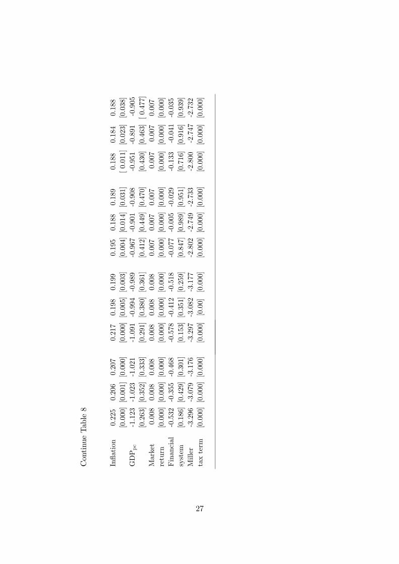
ContinueTable8
In�ation
0.225
0.206
0.207
0.217
0.198
0.199
0.195
0.188
0.189
0.188
0.184
0.188
[0.000][0.001][0.000]
[0.000][0.005][0.003]
[0.004][0.014][0.031]
[0.011][0.023][0.038]
GDPpc
-1.123
-1.023
-1.021
-1.091
-0.994
-0.989
-0.967
-0.901
-0.908
-0.951
-0.891
-0.905
[0.263][0.352][0.333]
[0.291][0.380][0.361]
[0.412][0.449][0.470]
[0.430][0.463][0.477]
Market
0.008
0.008
0.008
0.008
0.008
0.008
0.007
0.007
0.007
0.007
0.007
0.007
return
[0.000][0.000][0.000]
[0.000][0.000][0.000]
[0.000][0.000][0.000]
[0.000][0.000][0.000]
Financial
-0.532
-0.355
-0.468
-0.578
-0.412
-0.518
-0.077
-0.005
-0.029
-0.133
-0.041
-0.035
system
[0.186][0.429][0.301]
[0.153][0.351][0.259]
[0.847][0.989][0.951]
[0.716][0.916][0.939]
Miller
-3.296
-3.079
-3.176
-3.297
-3.082
-3.177
-2.802
-2.749
-2.733
-2.800
-2.747
-2.732
taxterm
[0.000][0.000][0.000]
[0.000][0.00]
[0.000]
[0.000][0.000][0.000]
[0.000][0.000][0.000]
27

Table9
Fixede¤ectpanelregressionestimatesfortheNorthAmericanregionbasedontheavailable�nancialinformation
ofall�rms.TherestrictedIPOproceedsandyearlyaggregatedvalueofall�rmspeci�cvariablesare
usedintheestimationprocess.ThetablereportsHACadjustedLSDVestimates
andp-valuesreportedinsquarebrackets.
Capitalgainincluded
Capitalgainincluded
Capitalgainexcluded
Capitalgainexcluded
withoutcountrye¤ect
withcountrye¤ect
withoutcountrye¤ect
withcountrye¤ect
�y it= 0+ 1�y it�1+ 2�(TopIncomeSharesit)+
n X i=3
i�(X
it)+e it
Paramater
IvP
Top
Top
IvP
Top
Top
IvP
Top
Top
IvP
Top
Top
Estimate
(�)
11/9
(�)
11/9
(�)
11/9
(�)
11/9
Intercept
-0.009
0.025
0.016
--
--0.018
0.042
0.014
--
-[0.923][0.771][0.874]
--
-[0.849][0.653][0.892]
--
-Lagofdependent
0.166
0.156
0.218
0.160
0.148
0.212
0.239
0.190
0.212
0.233
0.183
0.207
variable� y t�1
�[0.024][0.057][0.013]
[0.032][0.073][0.016]
[0.001][0.017][0.007]
[0.000][0.013][0.006]
Topincome
-0.640
-0.074
-1.510
-0.638
-0.075
-1.520
-1.087
-0.139
-3.101
-1.086
-0.141
-3.073
shares
[0.000][0.001][0.006]
[0.00]
[0.000][0.004]
[0.000][0.005][0.006]
[0.000][0.003][0.005]
SizeoftheFirm
-0.358
-0.759
-0.746
-0.633
-1.091
-1.063
-0.588
-1.156
-1.160
-0.873
-1.496
-1.395
[0.608][0.215]
[0.289]
[0.420][0.086][0.138]
[0.354][0.065][0.075]
[0.190][0.013][0.033]
Tangibility
0.854
0.509
0.605
1.000
0.700
0.785
-1.158
-0.446
-0.691
-1.002
-0.261
-0.561
[0.585][0.774][0.745]
[0.498][0.676][0.653]
[0.517][0.822][0.732]
[0.536][0.886][0.768]
Intangibility
3.367
3.083
3.570
3.736
3.532
4.000
2.747
3.190
3.163
3.132
3.645
3.483
[0.000][0.001][0.000]
[0.000][0.000][0.000]
[0.002][0.001][0.000]
[0.00]
[0.000][0.000]
Pro�tability
6.548
4.940
4.693
5.914
4.193
3.977
3.500
3.343
2.180
2.847
2.576
1.644
[0.012]
[0.036][0.058]
[0.027][0.067][0.102]
[0.167][0.146][0.348]
[0.278][0.247][0.488]
Sales
-0.606
-0.338
-0.468
-0.381
-0.061
-0.206
-0.338
-0.043
-0.095
-0.104
0.240
0.094
[0.457][0.674][0.619]
[0.661][0.938][0.821]
[0.648][0.954][0.903]
[0.887][0.725][0.899]
Liquidity
0.376
0.285
0.319
0.303
0.196
0.234
0.194
0.222
0.215
0.119
0.130
0.153
[0.040][0.086][0.089]
[0.160][0.289][0.244]
[0.241][0.171][0.200]
[0.542][0.444][0.400]
Marketrisk
0.037
0.030
0.032
0.037
0.030
0.032
0.038
0.032
0.031
0.038
0.032
0.031
[0.000][0.000][0.000]
[0.000][0.000][0.007]
[0.000][0.000][0.000]
[0.000][0.000][0.000]
28

ContinueTable9
In�ation
0.036
0.027
0.028
0.015
0.001
0.003
0.037
0.029
0.034
0.015
0.003
0.016
[0.391][0.502][0.551]
[0.766][0.967][0.940]
[0.371][0.518][0.487]
[0.725][0.941][0.746]
GDPpc
-0.975
-0.964
-0.812
-0.869
-0.837
-0.690
-0.597
-0.861
-0.604
-0.487
-0.733
-0.513
[0.000][0.000][0.000]
[0.000][0.000][0.008]
[0.019]
[0.001][0.021]
[0.099][0.012][0.089]
Market
-0.001
-0.001
-0.002
-0.001
-0.001
-0.002
-0.001
-0.002
-0.002
-0.001
-0.002
-0.002
return
[0.105][0.147]
[0.134]
[0.076][0.101][0.097]
[0.135][0.088][0.073]
[0.092][0.054][0.052]
Financial
-0.649
-0.664
-0.657
-0.664
-0.687
-0.678
-0.519
-0.580
-0.613
-0.536
-0.604
-0.624
system
[0.000][0.002][0.006]
[0.000][0.000][0.002]
[0.000][0.006][0.005]
[0.000][0.003][0.003]
Miller
-1.218
-1.188
-1.209
-1.198
-1.165
-1.187
-0.997
-1.071
-1.084
-0.977
-1.047
-1.068
taxterm
[0.001][0.001]
[0.003]
[0.001][0.000][0.003]
[0.000][0.000][0.008]
[0.000][0.000][0.001]
29

have retested our sample based on available �nancial information of issuing
�rms and recalculated the �rm speci�c factors based on yearly aggregated
value of �nancial information collected from the balance sheet of available
issuing �rms. The empirical �ndings are reported in Table-8. This analy-
sis recon�rms our hypothesis that top income shares negatively a¤ect the
leverage ratio of a �rm.
Another sample restriction is based on the price of IPOs and REITs
(Real estate investment trust) class of IPO issues. The restricted sample
includes IPOs with an o¤er price of at least $5.00, excluding all REITs
and all stocks not listed on Amex, NYSE, NASDAQ and Toronto stock
exchanges. The empirical �ndings based on the restricted sample are re-
ported in Table-9. Again our analysis recon�rms the hypothesis that the
relationship between top income shares and the leverage ratio of a �rm is
negative.
6 Conclusions
This paper has investigated the e¤ect of top income shares on the capi-
tal structure choice of a �rm. We �nd that the top income share is the
dominant factor in explaining the variation in leverage ratio for the �rms
of North American region. The negative relationship between top income
shares and leverage ratio found in the North American �rms but this re-
lationship is not present in �rms from other OECD countries. This paper
also uses information from �rm speci�c and macroeconomic variables (such
as, �rm size, tangibility, intangibility, pro�tability, sales, liquidity, market
risk, top income shares, in�ation rate, and economic growth rate, rate of
market return, �nancial system and Miller tax term) to explain the dynam-
30

ics of capital structure choice of OECD �rms. The result of this empirical
study provides some of the insights from modern capital structure theory.
The empirical evidences also reveal that certain �rm-speci�c and macro-
economic factors are relevant for explaining the capital structure choice.
However, a further investigation states that these traditional determinants
might not have the robust explanatory power in explaining the capital
structure choice. A larger, comprehensive, and more detailed database is
required for a further detailed capital structure study.
31

References
Atkinson, A. B., Piketty, T., (Eds.), 2007. Top Incomes over the Twentieth
Century: A Contrast between European and English-Speaking Countries.
Oxford University Press, Oxford.
Atkinson, A.B., and Leigh, A., 2010. The distribution of top incomes in �ve
Anglo-Saxon countries over the twentieth century. Institute for the Study
of Labor (IZA) Discussion Paper No# 4937.
Baker, M., and Wurgler, J., 2002. Market Timing and Capital Structure.
Journal of Finance 57, 1�32.
Banerjee, S., Heshmati, A. andWihlborg, C., 2004. The dynamics of capital
structure. Research in Banking and Finance 4, 275-97.
Bertrand, M., Du�o, E., and Mullainathan, S., 2004. How Much Should
We Trust Di¤erences-in-Di¤erences Estimates?. The Quarterly Journal of
Economics 119, 249-275.
Booth, L., Aivazian, V., Demirgüç-Kunt, A., and Maksimovic, V., 2001.
Capital structure in developing countries. Journal of Finance 56, 87-130.
De Jong, A., and Nguyen, T. T., and Kabir, R., 2008. Capital Structure
Around the World: The Roles of Firm- and Country-Speci�c Determinants.
Journal of Banking and Finance 32, 1954�1969.
Flannerya, M. J., and Hankins, K.W., 2013. Estimating Dynamic Panel
Models in Corporate Finance. Journal of Corporate Finance 19, 1-19.
Frank, M. Z., and Goyal, V. K., 2009. Capital Structure Decisions: Which
Factors are Reliably Important. Financial Management 38, 1-37.
32
Jensen, M., and Meckling, W., 1976. Theory of the �rm: managerial behav-
ior, agency costs and ownership structure. Journal of Financial Economics
3, 305-360.
Judsona, R. A., and Owen, A. L., 1999. Estimating dynamic panel data
models: a guide for macroeconomists. Economics Letters 65, 9�15.
Kacperczyk, M., Nosal, J. B., and Stevens, L., 2014. Investor Sophistication
and Capital Income Inequality. NBER Working Paper No. 20246.
Levine, R., 2002. Bank-based or market-based �nancial systems: Which is
better?. Journal of Financial Intermediation 11, 398-428.
Modigliani, F., and Merton H. M., 1958. The cost of capital, corporation
�nance, and the theory of investments. American Economic Review 48,
261-297.
Myers, S., 1977. The determinants of corporate borrowing. Journal of Fi-
nancial Economics 5, 147-175.
Nickell, S., 1981. Biases in dynamic models with �xed e¤ects. Econometrica
49, 1399�1416.
Piketty, T., Saez, E., 2007. Income inequality in the United States, 1913�
1998. In: Atkinson, Anthony B., Piketty, Thomas (Eds.), Top Incomes
over the Twentieth Century: A Contrast between European and English-
Speaking Countries. Oxford University Press, Oxford.
Rajan, R., and Zingales, L., 1995. What do we know about capital struc-
ture? Some evidence from international data. Journal of Finance 50, 1421-
1460.
33

Titman, S., and Wessels, R., 1988. The determinants of capital structure.
Journal of Finance 43, 1-19.
34