capturing dynamic effects in ship tanks - chalmers...
TRANSCRIPT

Capturing Dynamic Effects in Ship Tanks - A coupling between HydroD™ and OpenFOAM® Master of Science Thesis in Naval Architecture JACQUELINE ANDERSSON JONAS PEDERSEN Department of Shipping and Marine Technology Division of Sustainable Ship Propulsion CHALMERS UNIVERSITY OF TECHNOLOGY Gothenburg, Sweden, 2011 Report No. X-11/259


i
A THESIS FOR THE DEGREE OF MASTER OF SCIENCE
Capturing Dynamic Effects in Ship Tanks - A coupling between HydroD™ and OpenFOAM®
JACQUELINE ANDERSSON
JONAS PEDERSEN
Department of Shipping and Marine Technology CHALMERS UNIVERSITY OF TECHNOLOGY
Gothenburg, Sweden 2011

ii
Capturing Dynamic Effects in Ship Tanks - A coupling between HydroD™ and OpenFOAM® JACQUELINE ANDERSSON JONAS PEDERSEN © JACQUELINE ANDERSSON & JONAS PEDERSEN, 2011 Report No. X-11/259 Department of Shipping and Marine Technology Chalmers University of Technology SE-412 96 Gothenburg Sweden Telephone +46 (0)31-772 1000 Printed by Chalmers Reproservice Gothenburg, Sweden, 2011

iii
Capturing Dynamic Effects in Ship Tanks -A coupling between HydroD™ and OpenFOAM® JACQUELINE ANDERSSON JONAS PEDERSEN Department of Shipping and Marine Technology Division of Sustainable Ship Propulsion Chalmers University of Technology
Abstract When a ship with partially filled tanks is subjected to waves with frequencies in the vicinity of the natural period of the fluid inside the tanks, sloshing occurs. Sloshing influences the seakeeping properties of a ship but can be hard to capture when using softwares in seakeeping. DNVs software HydroD has this problem and cannot capture the dynamic forces from the tank, as it is today. The dynamic forces can be captured by using CFD and that is why a coupling between HydroD and a CFD software is interesting to investigate. By using already existing CFD software, that is able to give these dynamic forces as a force input, the problem might get solved. If choosing OpenFOAM which has the advantage of being easy available and free, it could also be beneficial from an economical point of view, since it would cost DNV more to develop a CFD feature in HydroD than using this software. The idea was to run HydroD initially to get a motion output from a barge model that would be used as motion input for the tank simulated in OpenFOAM. In turn, OpenFOAM would output forces to be used as force input in HydroD. This data exchange between the two programs would make an iterative process that would go on until the motion in HydroD converged. When investigating this problem, the results were verified against a known experiment where a model of a barge with a tank was subjected to beam sea and free to move in sway, heave and roll. Two particular cases were studied, one where the tank had no free surface effect and could be considered “closed”, and one where the tank was partially filled having a free surface. For the case without any free surface, results agreed well with the experimental one but for the case where there was a free surface present, the results were not as satisfying. Still, these results gave an indication that it could be possible to use OpenFOAM together with HydroD, but unfortunately time was a restricting factor which is why further work will be needed for obtaining better agreement, as described in recommendations.

iv
Sammanfattning När ett fartyg med delvis fyllda tankar utsätts för vågor med frekvenser nära vätskans naturliga period, uppstår en våldsam vågrörelse i tankarna. Detta fenomen påverkar ett fartygs sjöegenskaper, men kan vara svårt att prediktera med hjälp av programvara avsedd för beräkning av fartygets rörelser. DNVs programvara HydroD har detta problem och kan idag inte ta hänsyn till de dynamiska krafterna som fås från tanken. De dynamiska krafterna i sig, kan beräknas med hjälp av CFD och därför skulle en så kallad koppling mellan HydroD och en CFD-programvara kunna vara intressant att undersöka. Genom att använda en CFD-programvara för att ta reda på tankens krafter, skulle HydroD kunna ges dessa och därmed göra en bättre beräkning av fartygets verkliga rörelse. Om dessutom CFD programvaran OpenFOAM valdes, vilken är lätt tillgänglig och inte kostar något, kunde det vara fördelaktigt även ur en tidsmässig och ekonomisk synvinkel, eftersom det skulle kosta DNV mer att utveckla en CFD funktion i HydroD, än att använda detta program. Idén var att en modell av fartyget i HydroD skulle köras initiellt för att ge rörelser i tiden som utdata. Dessa utdata skulle användas av OpenFOAM som indata för simuleringen av tanken. OpenFOAM skulle i sin tur ge utdata i form av krafter vilka skulle användas som indata i HydroD för nästa simulering av fartyget. På så vis skulle dessa program köras i en iterativ process tills dess att rörelsen i HydroD konvergerade. De erhållna resultaten kom till att verifieras mot ett känt experiment där en pråmliknande modell med en tank använts. Denna modell hade utsatts för vågor med riktning ortogonalt mot modellens longitudinella axel där den tillåtits röra sig i tre frihetsgrader. Vid verifiering mot de experimentella resultaten undersöktes speciellt två fall. Ett utan påverkan av den fria vätskeytan från tanken, det vill säga att tanken kunde ses som stängd och ett fall med en delvis fylld tank vilken hade en fri vätskeyta. För den ”stängda” tanken erhölls överensstämmande resultat jämfört med de experimentella. Resultaten från fallet med fri vätskeyta var inte lika överensstämmande men gav en indikation på att det skulle kunna vara möjligt erhålla lyckade resultat även för detta fall. En begränsande faktor var tiden, varför rekommendationer om vidare arbete för att åstadkomma bättre resultat finns beskrivet under slutsatser och diskussion.

v
Preface This report is the result of a Master Thesis Project which was carried out as part of the Master Program in Naval Architecture at Chalmers University of Technology in Gothenburg, Sweden. The aim of the Thesis was to investigate if sloshing in tanks could be accounted for when coupling a software called HydroD to a CFD software. The work was carried out at the DNV office in Høvik, Norway, at the department DNV Software. Special thanks are given to the supervisors KaiJia Han, Peter Pan and Torgeir Vada at DNV Software but also to Associate Professor Rickard Bensow at the department of Shipping and Marine Technology, Chalmers University of Technology in Gothenburg, Sweden for suggestions and discussions. Høvik, May 2011 Jacqueline Andersson Jonas Pedersen

vi
Notations and Conventions CD Central Differencing Scheme CFD Computational Fluid Dynamics CoG Center of Gravity D Moment of Deviation DNS Direct Numerical Simulation DNV Det Norske veritas FP Forward Prependicular FPSO Floating Production Storage and Offloading vessel FVM Finite Volume Method GM Metacentric Height JONSWAP Joint North Sea WAve Project LNG Liquid Natural Gas OpenFOAM Open Field Operation and Manipulation RAO Response Amplitude Operator UD Upwind Differencing Scheme VoF Volume of Fluid

vii
List of Contents Abstract…… ............................................................................................................................. iii!Sammanfattning ........................................................................................................................ iv!Preface……. ............................................................................................................................... v!Notations and Conventions ....................................................................................................... vi!List of Contents ........................................................................................................................ vii!1.! Introduction ............................................................................................................ 1!
1.1! Free surface and sloshing effect ............................................................................. 1!1.2! Coupling HydroD™ and OpenFOAM® ................................................................ 1!1.3! Scope ...................................................................................................................... 1!1.4! Work Procedure ..................................................................................................... 2!
2! Theory .................................................................................................................... 3!2.1! HydroD™ and Wasim ........................................................................................... 3!2.2! OpenFOAM® ........................................................................................................ 5!2.3! Ship Motions .......................................................................................................... 8!
3! Method ................................................................................................................. 10!4! Model Description ............................................................................................... 10!
4.1! Barge Experimental Results ................................................................................. 10!4.2! Barge Model in HydroD™ .................................................................................. 12!4.3! Tank Model in OpenFOAM® ............................................................................. 14!
5! Verifications of Models ....................................................................................... 15!5.1! Verifying settings in HydroD™ ........................................................................... 15!5.2! Ship Motion Control ............................................................................................ 16!5.3! Mesh Convergence in HydroD™ ........................................................................ 17!5.4! Mesh Convergence in OpenFOAM® .................................................................. 20!5.5! Verifying of Tank Model in OpenFOAM® ......................................................... 20!5.6! 2D or 3D in OpenFOAM® .................................................................................. 21!
6! Coupling ............................................................................................................... 23!6.1! Coordinate transformation ................................................................................... 23!6.2! Handling Mass in Tank ........................................................................................ 26!6.3! Closed Tank Coupling ......................................................................................... 28!6.4! Tank Added Mass and Damping .......................................................................... 28!
7! Validation ............................................................................................................. 30!7.1! Closed Tank ......................................................................................................... 30!7.2! Open Tank ............................................................................................................ 31!7.3! Added mass and damping for the tank ................................................................. 33!
8! Discussion and Conclusion .................................................................................. 36!8.1! Sources of error .................................................................................................... 36!8.2! Recommendations ................................................................................................ 37!
References…. ........................................................................................................................... 38!Appendix A - Code from OpenFOAM® ................................................................................. 39!Appendix B - Code from Scripts .............................................................................................. 50!Appendix C – Drawing ............................................................................................................ 55!

viii

1
1. Introduction The main purpose of this Master’s Thesis has been to investigate a method for capturing the free surface effect, that may occur in tanks onboard ships, and how the seakeeping properties are influenced because of this effect. The aim has been to see whether the method is a possible way for obtaining more accurate results by usage of predetermined CFD software.
1.1 Free surface and sloshing effect A ship at sea with partially filled tanks will have its seakeeping properties influenced because of the motion inside the tanks. Even relatively calm sea may cause large displacement inside tanks and might create breaking waves, so called sloshing, inside it. The motion inside tanks may cause large drift forces and moments, depending on size, filling ratio and geometry. Only a small motion of the ship is needed to cause violent motion inside the tanks if the ship motion is close to the tank natural frequency. Especially this can be a problem for ships that are on and off loading where keeping the same position is crucial. The demand to simulate these effects has increased over the last years since LNG tankers and FPSO units, experiencing this problem, have become more widely used.
1.2 Coupling HydroD™ and OpenFOAM® Today, when seakeeping properties of a ship are to be investigated, the DNV developed program called HydroD can be used. This software does not calculate the dynamics inside the tank but treats the mass inside it as a solid body. Although, it is possible to take the free surface effect into account when calculating the hydrostatic stiffness matrix. One possible way to simulate the dynamics inside the tank may be to use a CFD software to calculate fluid motions and forces from inside the tank. If it is possible to use result from the CFD software as input into HydroD, i.e. account for dynamic effects, then it is also possible to gain more accurate results. Since DNV does not provide a CFD solver developed on their own, an external software needs to be used. From a commercial point of view this should be a reliable, easy available and preferably a free license one. OpenFOAM is such a software and was thought to be used for this purpose. Provided that a so called coupling where these two programs exchange data is possible, the customers that use HydroD could get results due to sloshing on their own and in a more accurate way, without purchasing a CFD program. From a general point of view, obtaining more accurate results would enable a better understanding of the ship behavior at sea and therefore improved design and safety of the ship.
1.3 Scope The scope of this Master Thesis was to investigate whether it was possible to couple HydroD and OpenFOAM in order to simulate ship motions, including free surface effects, more accurately. Problems associated with the coupling were to be stated together with possible solutions, if any. Further, the scope of this thesis included these two programs and no deep investigations among other softwares available for the intended purpose. This thesis has its focus on simulating the influence of the free surfaces, not minimizing nor reducing their effect. No effort was made to develop the programs themselves. The thesis was to be completed within twenty weeks, including time for planning, research, simulations, report writing and presentation.
2
1.4 Work Procedure Before the trials of coupling started some preparations were necessary. First of all, some literature was studied. Mainly papers on the topic were studied but also theory behind the softwares. Some time was also spent on investigation to find a suitable solver for the multiphase problem of the tank. After this, tutorials regarding the set up of a ship motion simulation in HydroD and 2D/3D sloshing cases for a tank in OpenFOAM were made, to learn these programs properly. A comparison between results from a tank in 2D and 3D was made to decide which one would be the most suitable when coupling. Finally, with a geometry model of the barge in HydroD, identical to the one from a known experimental case, an identical case was set up with the same settings and conditions. The results from the experimental case were to be used throughout the project to verify the motion response of the barge with a tank. When coupling, it was thought to simulate the motion of the barge in HydroD and use that motion time history as input for the motion of the tank in OpenFOAM. In OpenFOAM the time history of the forces inside the tanks was to be calculated and sent back to HydroD. This was to be done until convergence of the motion in HydroD was reached.

3
2 Theory In this chapter a short introduction of the theory behind the softwares is presented together with theory regarding Ship Motions. This is a brief introduction and does not intend to fully cover all features and settings available in the two programs, but mainly describes the ones used.
2.1 HydroD™ and Wasim HydroD is a software, developed by DNV, for hydrostatic and hydrodynamic analysis. It performs seakeeping and wave load analysis. Wasim is the solver used in HydroD that computes the global force, motion and local loading on vessels moving forward at any speed for displacing hulls. In more precise words, it computes, from a given incoming wave or wave spectrum, displacement, velocity and acceleration and how these affect the motion in the six degrees of freedom (surge, sway, heave, roll, pitch and yaw) by calculating motion response amplitudes. Also, it computes global forces and sectional loads. In Wasim the simulations are made in the time domain but can be Fourier Transformed into the frequency domain. What the program solves is a fully 3-dimensional radiation/diffraction problem. The problem is solved by Potential Flow Theory and by use of the Rankine Panel Method where panels are used on both hull and surface. These panels build up the model where each panel is assigned a so called Rankine Source. This source with a certain strength is defined as a point where the velocity vector of the fluid is in the radial direction.
2.1.1 Potential Flow An approximation of the flow around a body in water is that the flow field can be divided into two regions, one outer and one inner surrounding the body. In the outer region the viscosity can be neglected but the inner one is dominated by viscous forces. In potential flow theory it is assumed that the inner region is very thin and small compared to the outer one which is why all viscosity can be neglected. It is also assumed that the flow is incompressible and irrotational.
2.1.2 Potential Flow with Free Surface Below, water approaches the hull with the undisturbed speed, ∞U . The coordinate system is located at the forward perpendicular, FP, according to figure 2.1.
Figure 2.1: Picture of the hull described above. Janson (2008).
Consider a small control volume of fluid where the flow is incompressible. The continuity equation for potential flow yields the Laplace equation where φ is the velocity potential.

4
2
2
2
2
2
2
0zyx ∂∂
+∂∂
+∂∂
=φφφ
(2.1)
Equation (2.1) is a linear differential equation of second order. All harmonic wave components with different amplitudes, frequencies and phases can be superposed to obtain the total solution giving motion, velocity and acceleration of the fluid particle. For obtaining pressure and water levels, the Bernoulli equation needs to be used. This Bernoulli equation is valid for irrotational, incompressible, three-dimensional and stationary flow. Here, C is a constant and η is the wave height
))()()((5.0 222
zyxpgC
∂∂
+∂∂
+∂∂
++=φφφ
ρη (2.2)
In order to solve for η and φ some boundary conditions are needed. The first boundary condition is due to that the flow through the hull surface is zero
0)( =∂
∂hsn
φ (2.3)
Here index hs means hull surface and n is the normal vector. Also, far from the hull, the velocity will be undisturbed
∞∞→
=∇ Ur
φlim (2.4)
When there is a free surface two more boundary conditions are needed. First, the velocity in the normal direction of the free surface is assumed zero.
0)( =∂
∂fsn
φ (2.5)
where index fs stands for free surface. The static pressure on the free surface is also assumed constant with a reference pressure set to zero. Hence the Bernoulli equation becomes
))()()((5.00 2222∞−
∂∂
+∂∂
+∂∂
+= Uzyx
g φφφη (2.6)
To find η and φ this free surface problem can be solved by linearizing around a known base solution where the total velocity potential is expressed as a basis flow potential φ 0 and a disturbance flow potential φ 1 so that φ = φ 0 + φ 1. In the same manner the wave elevation is expressed as η= η0+ η1. Kurultay((2003).

5
2.1.3 Rankine Panel Method Wasim uses the Rankine Panel Method which solves for the flow passing around an arbitrarily shaped body in 2D and 3D. The surface of the body and free surface is divided into N number of panels where each panel has a time varying source strength A system of N linear equations is set up to solve for . When the source strength is known, the pressure and velocity for each panel can be determined. When setting up the linear equation system Greens function which satisfies the free surface boundary conditions, is used. Kurultay((2003). The velocity potential φ (x) is to be determined over the mean translating position of the hull SB and over the free surface SF. The Laplace equation (2.1) for the fluid domain bounded by SB and SF can be set up by use of the Greens Theorem for the Rankine Source potential
),( ξxG and the velocity potential φ (x) as
ξπξ
−=
xxG
21),( (2.7)
This leads to an integral relation between φ (x) and the normal derivative of φ n(x) over SB and SF where φ n is known and comes from the body boundary condition over SB. Kurultay((2003).
ξξξφ
ξξξφφξξ
dxGntdx
nGttx
BFBF SSSS
),(),(),(),(),( ∫∫∫∫++ ∂
∂−
∂∂
+ (2.8)
2.2 OpenFOAM® The motion of the fluid inside a tank may be quite violent and result in breaking waves. Today it is not possible to simulate this behavior with HydroD and even if it was, Potential Flow Theory would not be feasible when breaking waves and viscous effects occur inside the tank. With a CFD tool it is possible to simulate the behavior of the internal fluid. The accuracy of the result will be influenced by choice of model, mesh size, mesh distribution, chosen boundary conditions and chosen solver. The model in this case represents the mathematical description of the physical object that should be simulated, while the solver specifies the procedure for obtaining an approximate result to the equations. For simulation of the fluid motions in the tanks for this thesis, a CFD program called OpenFOAM (version 1.6.x), Open Source Field Operation and Manipulation, was used (www.openfoam.com). As the name reveals, OpenFOAM is an open source program and it is free of charge and the user can easily get access to the code that builds up the program. In order to solve a problem, a solver that is designed for that specific problem is used. OpenFOAM has a number of pre-built solvers but it is also possible for the user to design their own if necessary, or manipulate an existing one. However, since OpenFOAM is a C++ library, some basic knowledge in object oriented programming is required in such case. To get the most accurate result a solver that solves the Navier-Stokes equation completely should be used. DNS, Direct Numerical Simulation, is such a method where the Navier-Stokes equation is solved without any simplifications. The major drawback is the large computational cost. Today it is not feasible to use DNS in most engineering and it is therefore

6
only used for small applications and in research. Further, the details provided by the Navier-Stokes equation are normally not necessary in engineering applications and therefore, it is possible to do some simplifications. When using RANS, the flow velocity are decomposed into a mean flow velocity and a turbulent quantity. This is done by time averaging over a reasonable time period. In practice, this time period will be larger than turbulent time scales. In Navier-Stokes equation an additional term, due to the unknown fluctuation apart from the mean flow, will be introduced, called Reynolds Stresses. To solve the equation with Reynolds stresses, turbulence models can be used. Although, for the application in this thesis the viscous effects due to turbulence are considered to have small affect on the result. Hence, no turbulence model was used. Andersson et al (2010). The outputs obtained from OpenFOAM are velocity, pressure and phase fraction, wall pressures and pressures at specified locations. What can also be obtained are forces and moments. Moments are calculated by multiplying the force with the distance to the user specified centre of rotation. Vectors for force and moments are obtained in pressure and viscous components.
2.2.1 Solver When sloshing occurs it is possible that wave breaking and mixture with surrounding air will be a consequence. This implies the usage of a two phase solver. In order to simulate the two phase physics of this problem, a solver for two incompressible fluids in the OpenFOAM package called interDyMFOAM can be used. It uses the Volume of Fluid Method (VoF) which is a phase-fraction based interface capturing approach where mass of the tracked fluid is conserved, see chapter 2.2.3. In VoF, the surface interface is tracked by using a phase fraction function. In this way, complex interface changes such as breaking or reconnecting surfaces can be captured. The Volume of Fluid Method is not a standalone flow solving algorithm and therefore the Navier Stokes equations are solved separately using the Finite Volume Method. InterDyMFOAM provides the opportunity to use a dynamic mesh. The solver can re-mesh between each time-step depending on the movement of the fluid.
2.2.2 Schemes A scheme is used to determine how the interpolation, between the control volumes, should be made. The selection of numerical schemes will have great influence on the simulation result. In OpenFOAM it is possible to specify different schemes for different terms that are calculated during simulations. This gives the user great freedom but on the other hand it requires some knowledge in order get good result. It is out of scope for this project to explain all available schemes but in the following chapters a brief explanation of schemes used is made.
2.2.3 Finite Volume Method with Volume of Fluid Method By usage of FVM, a continuous equation such as the transport equation of the flow is discretized by dividing the space domain into a number of so called control volumes or cells. It is also possible to discretize in time to get the time domain dependencies. In the space domain, the control volumes are bounded by faces. The faces between each cell are called internal faces while the faces facing the outer boundary are called boundary face. The dependent variables can either be stored at the centre of each cell or at the face center. In most CFD codes, the first option is used. Interpolation of the values in the center of each volume to its face centers is important in FVM and can be done by using different schemes. The choice of scheme is important since this, together with mesh, will determine the accuracy, stability

7
and to some extent also the convergence of the simulation. Most common schemes are the Central Differencing Scheme (CD), the Upwind Scheme (UD) and the Hybrid Scheme that uses either CD or UD depending on the flow. Jasak (1996). The governing equation for an incompressible fluid is the Navier-Stokes equation. Since the fluid is considered incompressible and mass is conserved, the continuity equation must also be valid. Then the Navier-Stokes and equation for incompressible Newtonian fluids can then be written
( )
0=U
Uυ+pρ1=UU+
tU
⋅∇
∇⋅∇∇−∇⋅∂
∂
(2.9)
In the FVM, this equation is integrated over the control volumes. When two fluids are present, as in the case of sloshing, this phenomenon needs to be accounted for in the discritisation of the cells. One way of doing this is to introduce the volume fraction, γ, to capture the interface between the two fluids. γ will be equal to one in a point where only one of the fluids are present and equal to zero when only the other fluid is present. A value of γ between one and zero indicates a mixture of the fluids. The scheme used in this Master Thesis for tracking the interface is a so called Weller Scheme, Rusche (2002), where the third term on the left hand side has been added to the so called indicator function below.
( ) ( )[ ] 0=γ1γU+Uγ+tγ
r −⋅∇⋅∇∂
∂ (2.10)
Here rU is a velocity field that is multiplied by )1( γγ − . This multiplication yields that the term will influence only in the interface region, which is normally very thin. The continuity equation reads
( ) 0=γU+tγ
∇⋅∂
∂ (2.11)
The local density and local viscosity are given by ( )( ) ba
ba
υγ1+γυ=υργ1+γρ=ρ
−
− (2.12)
where a and b are the different fluids present in the system. Further, also the surface tension, acting on the interface between the fluids, needs to be included into the equations. The shape and location of the surface is unknown but the surface tension is approximated to γσκ∇ where κ is the curvature of the interface, Rusche (2002)
| |!!"
#$$%
&
∇
∇⋅∇
γγ=κ (2.13)
With these modifications and some boundary conditions the momentum equation (2.9) becomes
( ) ( ) ( ) γσκ+ρhgυU+Uυ+p=ρUU+ρa+tρU
F ∇∇⋅−∇⋅∇∇⋅∇−∇⋅∇∂
∂ (2.14)

8
which is the equation to be discretized over the cells and aF is the acceleration of the moving reference frame, Rusche (2002).
2.3 Ship Motions A free floating ship is free to move in six degrees of freedom. These are surge (ξ1), sway (ξ2), heave (ξ3), roll (ξ4), pitch (ξ5) and yaw (ξ6). The coordinate system shown in figure 2.2 is well known for marine applications and also the one mainly used throughout this report.
Figure 2.2: Coordinate system with the six degrees of freedom in translation and rotation, Benedict et al.
The equation of motion for a ship, free to move in six degrees of freedom can be written as:
FCBAM =+++ ξξξ )( (2.15) Here M, A, B and C are 6x6 matrixes of mass, added mass, radiation-damping and hydrostatic stiffness respectively. ξ and F are 6x1 vectors, Dai (1998).
!!!!!!!!!!!
"
#
$$$$$$$$$$$
%
&
−
−
−−
−
−=
664
5
464
000
0000
00
0000
0000
000
ID-my
Imz
DImymz
mym
mzm
-mymzmM
g
g
gg
g
g
gg
(2.16) Here m is the total mass of the ship and yg and zg are the horizontal and vertical distance respectively to the center of gravity for the ship. D46 and D64 are the moments of deviation of the ship while I4, I5 and I6 are the mass moment of inertia around the axis. The same configuration of the mass matrix can be used to describe a ship including a tank or a ship and tank separately to be superposed. Mass moment of inertia for the tank, if treated as a solid body, can be calculated by.
( ) 2224 12
1 mdhbmI ++= (2.17)
Where m is the mass of the content in the tank, b and h are the breath and height of the tank. d is the orthogonal distance from center of the tank to the axis where I4 is calculated. The coefficients of the A and B matrixes are functions of the frequency of the motion caused by the generated waves around the ship. The coefficients of the added mass matrix are also

9
functions of shape of the ship. Although, as , the added mass becomes independent on the frequency. Also, far from the free surface the added mass is constant and depends only on the shape of the ship. The radiation or hydrodynamic damping is due to the energy of the waves transported away caused by the oscillating ship motion. For a floating body, the radiation damping becomes zero as and . The hydrostatic stiffness or so called restoring matrix C is due to the change of displacement and describes how hard it is to change the position of the ship. If the ship is at zero speed, the added mass and damping matrixes becomes symmetrical, see equations below. This also requires that ship can be considered symmetrical at both starboard/port and fore/aft. Bergdahl (2010).
!!!!!!!!!!
"
#
$$$$$$$$$$
%
&
66
5551
4442
33
2422
1511
A00000
0A000A
00A0A0
000A00
00A0A0
0A000A=A (2.18)
!!!!!!!!!!
"
#
$$$$$$$$$$
%
&
66
5551
4442
33
2422
1511
B00000
0B000B
00B0B0
000B00
00B0B0
0B000B=B (2.19)
!!!!!!!!!
"
#
$$$$$$$$$
%
&=
000000
0C0C00
00C000
0C0C00
000000
000000C
5553
44
3533
(2.20)

10
3 Method The method was to investigate if OpenFOAM could be used with HydroD to capture the dynamic effects from the tank that HydroD cannot capture today. To verify that reasonable results were obtained, a known experimental case from Molin (2008) and Molin (2002) was used, see chapter 4.1. When coupling, the barge was first simulated in time domain in HydroD, giving motion output in three degrees of freedom for a predefined point, which was chosen as the center of gravity for the whole system, also called motion reference point. This motion file was processed through a script to obtain the right syntax for OpenFOAM motion input. The tank with fluid in OpenFOAM was simulated with these motions in time given at the corresponding point in OpenFOAMs coordinate system. OpenFOAM then produced forces for this point that had to get processed through another script, becoming a so called auxiliary force that was used as input for next simulation in HydroD. This procedure went on until convergence was observed for roll Response Amplitude Operator, RAO, which is the ship motion divided by the amplitude of incoming wave. The reason for having a processing script between the programs was not only that the programs require its input in a specific syntax but also that the coordinate system in HydroD was body fixed (i.e. it follows the barge when it moves) and OpenFOAMs coordinate system was earth fixed.
4 Model Description
4.1 Barge Experimental Results To verify the numerically obtained results, a suitable known experiment Molin et al (2002) was used. This was an experiment where a barge with two rectangular tanks mounted symmetrically fore and aft of the midsection on the deck, was submitted to beam sea. The sea condition was an irregular JONSWAP spectrum with peak enhancement factor, γ=2 and a peak period, Tp, of 1.6 seconds. The JONSWAP spectrum is used to describe the wave distribution when using a North Sea wave condition. From this experiment, values of the RAO of wave and ship motion were obtained. The experiment was carried out a in a basin with the tanks placed with their length in the transverse direction of the barge. The internal bottom was placed 0.3 m above the keel line and mass of the barge with empty tanks was 169 kg with a CoG at 0.24 m above keel. The tests were carried out at draft 0.108 m which corresponds to a displacement of 285 liters. The barge was anchored to the walls by 4 lines and the motion of the water inside the tanks was measured with probes. The motion of barge was measured with an optical tracking system. Table 4.1 below shows the conditions for the barge experiment.

11
Table 4.1: Table for the conditions in Molins experiment. Settings and Conditions Barge Experiment
Model Unit Barge 3 x 1 x 0.267 [m] Tank 0.8 x 0.5 x 0.45 [m] Mass of Barge 169 [kg] CoG above keel 0.24 [m] Draft 0.108 [m] Filling Level of Tank 0.29 [m] Wave Conditions Unit Significant Wave height 1 0.06 [m] Significant Wave height 2 0.12 [m] JONSWAP Spectrum Wave Direction 90º
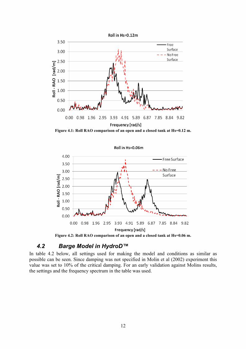
Properties of Air and Water Unit Air Density 1.226 [Kg/m^3] Kinematic Viscosity 1.46E-05 [m^2/s] Water Density 998 [Kg/m^3] Kinematic Viscosity 1.00E-06 [m^2/s] Water Depth Infinite [m] Model Basin Length 40 [m] Breadth 16 [m] Depth 3 [m] Figure 4.1 – 4.2 shows results for the roll RAO with the filling level of 0.29 m and significant wave heights of 0.06m and 0.12m respectively. In figure 4.1 and 4.2 there is a gap of 0.16m between water surface and roof of tank for one of graphs which in this thesis is referred to as an open tank. For the other graph in figure 4.1 and 4.2 there is no gap between water and roof and hence no effect from a free surface, which is considered a so called closed tank. What can be observed is that when having a free surface, a second peak in roll RAO is obtained. Noticeable is also that the second peak is lower when significant wave height is increased. For the case with 0.12 m significant wave height, the water hits the roof and that will cause some damping of the fluid motion in the tank which causes the decrease in peak height.
12
Figure 4.1: Roll RAO comparison of an open and a closed tank at Hs=0.12 m.
Figure 4.2: Roll RAO comparison of an open and a closed tank at Hs=0.06 m.
4.2 Barge Model in HydroD™ In table 4.2 below, all settings used for making the model and conditions as similar as possible can be seen. Since damping was not specified in Molin et al (2002) experiment this value was set to 10% of the critical damping. For an early validation against Molins results, the settings and the frequency spectrum in the table was used.

13
Figure 4.3: View of the barge model with tank and the surrounding surface that were used for simulations in HydroD/Wasim. Table 4.2: Table for the conditions in HydroD.
Conditions and Settings for the Barge in HydroD Model Unit Frequency Set [rad/s] Barge 3 x 1 x 0.267 [m] 2 Tank 0.8 x 0.5 x 0.45 [m] 3 Mass of Barge 169 [kg] 3.5 Filling Level of Tank 0.29 [m] 4 4.125 Wave Conditions Unit 4.25 Significant Wave height 0.06 [m] 4.5 Direction 90° 4.625 Frequency (for time domain) 6 [rad/s] 4.75 Damping 10% 5 5.5
Properties of Air and Water Unit 6 Air 6.5 Density 1.226 [Kg/m^3] 7 Kinematic Viscosity 1.46E-05 [m^2/s] 7.5 Water 8 Density 998 [Kg/m^3] 8.5 Kinematic Viscosity 1.004E-06 [m^2/s] 9 Water Depth Infinite [m] 9.5 10
Simulation Settings Unit Motion Free Motion Roll Velocity 0 [m/s] Time Step 0.01 [s] Duration 100 [s] Linearization Method Double body Integration Method First Order Analysis Type Linear

14
4.3 Tank Model in OpenFOAM® OpenFOAM provides a number of solvers for multiphase flow and the reason why InterDyMFOAM was chosen was because a solver that could handle the two present phases, air and water and move its mesh, was required. Also, there was no time to investigate alternative multiphase solvers. InterDyMFOAM uses a dynamic mesh, which means that the mesh is moving depending on the movement of the tank. In the tutorials for sloshing, the same solver was used which simplified the set up when coupling. The size of the tank used for the simulations were of the same dimensions as the one used by Molin (2008). In figure 4.4 the tank can be seen.
Figure 4.4: The tank model, its dimensions and mesh used in OpenFOAM.
The tank was filled with fresh water up to 0.29 m. During coupling, a 2D mesh with one cell in length, together with the boundary condition empty back and front was used. In this way, OpenFOAM was manipulated to think that it was a 2D case. The advantage of running simulations in “2D” rather than 3D was faster simulations and still sufficiently accurate results. If the forces from a “2D” case were multiplied by the length of the tank, they agreed well with the forces from a 3D case, see chapter 5.6. Optimization and validation of the mesh density was made to find that results were accurate enough if a mesh size of one cell per centimeter was used, see chapter 5.4. For motion input the Sea Keeping Analysis tool was used. This tool will move the mesh according to the motion input file. By using an OpenFOAM library called libforces.so forces and moments could be obtained as output. What happened in OpenFOAM was that the pressure of an area was integrated to obtain these moments and forces. Both forces and moments were specified at every output time. It was chosen to have the same output time as the time step in HydroD which was 0.01 s. The properties of the water inside the tank were set to a density of 998 kg/m3 and viscosity of 10-6 kg/(s·m) Regarding schemes the default ones from previous made tutorials in sloshing were chosen, see Appendix A.
0.8 m
0.29
0.45

15
5 Verifications of Models
5.1 Verifying settings in HydroD™ To verify that the model and its settings in HydroD was as similar as possible to Molins (2002/2008) experiment regarding for instance dimensions of barge and tank, properties of fluids, sea condition, mass, damping and restoring forces, a case with free roll, sway and heave was run in the frequency domain and compared to Molins results. In figure 5.1 below it can be seen that for a tank without any free surface, the results from the experiment and HydroD agree well, which implies that the settings in HydroD seem correct. In a comparison between the curves for free surface effect, the actual problem that this Master Thesis aims to solve, is seen. HydroD cannot capture the second peak that was captured in the experiment. This is due to the fact that when the tank is open and HydroD takes the free surface effect into account, it only updates the restoring matrix C by reducing GM for some of the elements in it, which is a correction of the hydrostatics. A reduction of the restoring will give a lower RAO at the first peak and also shift it to the left according to figure 5.1. It still cannot capture the hydrodynamics from inside the tank as stated in chapter 1.2.
Figure 5.1: Roll RAO for the experiment by Molin [2008] and also obtained from HydroD. Results are shown both for including free surface effects and also without this effect.

16
5.2 Ship Motion Control For the ship not to drift away when exposed to waves as during the simulation, HydroD uses a motion control spring system that is visualized in figure 5.2. This motion control system is dependent on the mass and will calculate corresponding restoring and damping coefficients according to equation (5.1) and (5.2). The index i stands for the position (row, column) of the matrix in question.
)6,4,2,1(,)2/( 2 =
+= iT
AMCi
iiiii π
(5.1)
)6,4,2,1(,)2/(
22 == i
TCB
i
iii π
ζ (5.2)
M, A and C are the matrixes for mass, added mass and restoring respectively and it can be seen that if M is reduced, C will also get reduced. T is the eigenperiod of the spring and iζ is a damping coefficient. What also happens when the tank mass is not considered in HydroD, is that the eigenperiod of the barge changes and then also the restoring and damping forces that tries to keep the ships position will change and hence affect the resulting motion of the ship. Since it was not completely decided from the beginning, if the mass of the tank was to be kept in HydroD during simulations these springs were replaced by additional restoring and damping matrixes. Only B22, C22, B44 and C44 had to be changed since we only have roll sway and heave. The used values can be seen in equation (5.3).
Figure 5.2: Spring system of the barge in HydroD, Pan (2010), with stiffness and damping according to the equations below.

17
NmC N/m.C
Nsm.B Ns/m.B
142169112605550321780
44
22
44
22
=
=
=
=
(5.3)
5.3 Mesh Convergence in HydroD™ To make sure that the mesh for the free surface in HydroD was fine enough, a convergence check was made. A circular mesh with a radius of 5 ship lengths was made for the free surface. This mesh was refined closer to the hull with a radial stretching ratio of 1:4. Different meshes and their corresponding values of free motion in heave, sway and roll were compared to see when sufficient accuracy was obtained. Since roll motion was to be investigated in the coupling, this was evaluated for the mesh convergence. In these computations, the frequency set and sea condition declared in table 4.2 was used. In figure 5.3 below, a quite coarse mesh can be seen where there are 15 elements longitudinally along the barge, 10 elements in the transverse direction and 15 elements in the radial direction of the free surface mesh. This was the coarsest mesh investigated and it corresponds to the dashed curve in figure 5.4 below. As can be seen, in figure 5.6 it is not crucial for the roll RAO what mesh size that is used, even if it is rather coarse. But since it matters for the roll motion in time domain, a grid size of 30 elements along the side of the barge, 20 in its transverse direction and 30 elements in the radial direction of the surface was chosen. The stretching factor of 1:4 where the elements are smaller close to the barge, was kept. A comparison between the different grid sizes for the roll motion can be seen in figure 5.4 and 5.5. In figure 5.6 and 5.7 a comparison of the different grid sizes for RAO are shown.
Figure 5.3: Example of the surface mesh that is symmetric around the longitudinal axis of the barge. The mesh used was finer but had the same configuration. Radius equals five ship lengths.

18
Figure 5.4: Convergence check with roll motion in time.
Figure 5.5: Magnification of the roll motion in time

19
Figure 5.6: Convergence check with roll RAO in the frequency domain
Figure 5.7: Magnification of the roll RAO in frequency domain. Note that the colors do not correspond to the same mesh size for the plots in time domain and frequency domain.

20
5.4 Mesh Convergence in OpenFOAM® According to the figures 5.8 – 5.9 below, where the force in sway and heave has been investigated, it can be observed that as long as the coarsest mesh size of 30x40 elements was not chosen, all the other sizes would be adequate. The one chosen was a mesh of 60x80 elements where one cell has the size of one centimeter in each direction. This size corresponds to the red curve in the figure below.
Mesh Covergence Y-force
-260
-200
-140
-80
-20
40
100
160
220
29 31 33 35 37 39 41
Time [s]
Fo
rce
Y [N
]
30x4060x8075x100105x140
Figure 5.8: Comparison of the force in y for the open tank.
Mesh Convergence Z-force
-1400
-1350
-1300
-1250
-1200
-1150
-1100
-1050
-1000
-950
-900
13 15 17 19 21 23 25
Time [s]
Forc
e Z
[N]
b100xh75b40xh30b140xh105b80xh60
Figure 5.9: Comparison of the force in z for the open tank.
5.5 Verifying of Tank Model in OpenFOAM® To make sure that reasonable results would be obtained from simulations in OpenFOAM some validation of the sloshing modes was made. The result of these simulations should not be seen as proof of good accuracy by OpenFOAM but as a first check for reasonable results. What also was important to check was if the coupling between HydroD and OpenFOAM worked in the sense that the tank really moved in the way prescribed in the motion input file given. The natural frequencies were, for a rectangular tank, given by the following formula

21
h)(ktanhkg=ω nn
2n ⋅⋅ (5.4)
Here h is the water depth in the tank and kn is the wave number which is calculated according to equation (5.5) and n is an integer.
bnπ=kn (5.5)
Here b is the breath of the tank. With a filling height of 0.29 m in the tank the first natural sloshing frequency becomes 5.6 rad/s. According to theory, Bunnik (2010), half of a wave length should fit into the tank when the first sloshing mode occurs. For second sloshing mode, which occurs at 8.69 rad/s, a full wave length should be present inside the tank. Further, for the third sloshing mode, at 10.74 rad/s, one and a half wave length should fit into the tank. Figure 5.10 shows snap shots from OpenFOAM simulations in 2D and 3D at the first and third sloshing modes. The results show good accuracy according to theory. According to Bunnik (2010) the second sloshing mode is not directly excited by the motion of the tank, if it exist it is due to non-linear wave interaction inside the tank.
5.6 2D or 3D in OpenFOAM® As mentioned in chapter 4.3, it had to be decided whether a 2D or 3D model of the tank in OpenFOAM was to be used. Simulations with the same motion input as when coupling, i.e. beam sea with free motion in sway, heave and roll, was made. Results are presented in figures 5.11 – 5.13. As can be seen, there is not much difference between runs in the different dimensions regarding forces and moments. In Wasim, the barge model was free to move in sway, heave and roll only. For this reason, there is no comparison of the forces in for instance the x direction. Since differences regarding forces and moments were quite small when comparing 2D and 3D and computation time in 3D was considerably long, it was decided that a 2D model of the tank was to be used and then integrated over the length in x-direction.
Figure 5.10: The leftmost picture shows the first sloshing mode while the picture in the middle shows the third sloshing mode. The rightmost image shows the third sloshing mode in 3D.

22
Figure 5.10: Comparison between the force in y direction for a 2D and 3D model of the tank.
Figure 5.112: Comparison between the force in z direction for a 2D and 3D model of the tank.
Figure 5.12: Comparison between the roll moment for a 2D and 3D model of the tank.

23
6 Coupling In this chapter the necessary steps for coupling of the two softwares are described. This includes some coordinate transformation, handling of the tank mass, taking the added mass and damping from the tank into account and also a verification of a closed tank coupling without any free surface effect. When looking at a free floating ship with partially filled tanks that is exposed to external waves, the motion may be written as
sloshext F+F=C+B+A)+(M ξξξ (6.1)
ξ is the motion vector while Fext and Fslosh are vectors that each contains three forces and three moments. Fext represents the forces acting on the hull, caused by the external waves. Forces caused by sloshing in the tanks are represented by Fslosh. The external force consists of gravity forces, translation forces and moments caused by the waves.
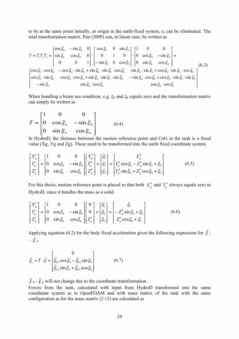
6.1 Coordinate transformation In OpenFOAM the coordinate system is always earth-fixed, but in HydroD/Wasim this is not always the case. HydroD/Wasim uses several different coordinate systems for different specifications. Among these there are two coordinate systems, one “Global System” and one “Body Fixed System” that have been used in this thesis. Briefly explained, the “Global System” is earth fixed while the “Body Fixed System” follows the motion of the body.
Figure 6.1: The picture shows the earth fixed and body fixed coordinate system and the relation between them. The motion output from HydroD is given in an earth-fixed system while velocity and acceleration are given in a body-fixed coordinate system. Since the auxiliary force from OpenFOAM should be given to HydroD in an earth-fixed system but must be calculated by using accelerations obtained in a body-fixed system these accelerations must be transformed. A position vector in earth-fixed system, re, can be expressed as
→→→
++= ξ0rrTr be (6.2) T is the transformation matrix, rb is a position vector in the body-fixed system, r0 is the translation vector between the origins for the two different systems and ξ is a vector containing the motion in x-, y- and z-direction. By choosing origin for the body-fixed system
ξ
r0
Z’
Y’’’
Z
Y
24
to be at the same point initially, as origin in the earth-fixed system, r0 can be eliminated. The total transformation matrix, Pan (2009) can, in linear case, be written as
!!!
"
#
$$$
%
&
⋅⋅−
⋅⋅+⋅−⋅⋅+⋅⋅
⋅⋅+⋅⋅⋅+⋅−⋅
=
!!!
"
#
$$$
%
&
−⋅
!!!
"
#
$$$
%
&
−
⋅
!!!
"
#
$$$
%
& −
==
54545
654646546465
654646546465
44
44
55
55
66
66
coscoscossinsinsinsincoscossinsinsinsincoscossincoscossincossinsincossinsinsincoscoscos
cossin0sincos0001
cos0sin010
sin0cos
1000cossin0sincos
ξξξξξ
ξξξξξξξξξξξξ
ξξξξξξξξξξξξ
ξξ
ξξ
ξξ
ξξ
ξξ
ξξ
xyz TTTT
(6.3)
When handling a beam sea condition, e.g. ξ5 and ξ6 equals zero and the transformation matrix can simply be written as
!!!
"
#
$$$
%
&
−=
44
44
cossin0sincos0001
ξξξξT (6.4)
In HydroD, the distance between the motion reference point and CoG in the tank is a fixed value (Xg, Yg and Zg). These need to be transformed into the earth fixed coordinate system.
!!!
"
#
$$$
%
&
++
+−=
!!!
"
#
$$$
%
&
+!!!
"
#
$$$
%
&
!!!
"
#
$$$
%
&
−=!!!
"
#
$$$
%
&
344
244
3
2
1
44
44
cossinsincos
cossin0sincos0001
ξξξ
ξξξ
ξ
ξ
ξ
ξξ
ξξbg
bg
bg
bg
bg
bg
bg
bg
eg
eg
eg
ZYZYX
ZYX
ZYX
(6.5)
For this thesis, motion reference point is placed so that both b
gX and bgY always equals zero in
HydroD, since it handles the mass as a solid.
!!!
"
#
$$$
%
&
+
+−=
!!!
"
#
$$$
%
&
+!!!
"
#
$$$
%
&
!!!
"
#
$$$
%
&
−=!!!
"
#
$$$
%
&
34
24
1
3
2
1
44
44
cossin0
0
cossin0sincos0001
ξξ
ξξ
ξ
ξ
ξ
ξ
ξξ
ξξbg
bg
bg
eg
eg
eg
ZZ
ZZYX
(6.6)
Applying equation (6.2) for the body fixed acceleration gives the following expression for ξ 1 – ξ 3
!!!
"
#
$$$
%
&
+
−=⋅=
4342
4342
cossinsincos
0
ξξξξ
ξξξξξξ
bb
bbe T (6.7)
ξ 4 - ξ 6 will not change due to the coordinate transformation. Forces from the tank, calculated with input from HydroD transformed into the same coordinate system as in OpenFOAM and with mass matrix of the tank with the same configuration as for the mass matrix (2.13) are calculated as

25
!!!!!!!!
"
#
$$$$$$$$
%
&
++−+−⋅+⋅−
−++⋅
+⋅−−⋅
=⋅=
00
)cossin)(sin()sincos()cos()sin()cossin()cos()sincos(
0
44434242434234
4424342
4344342
ξξξξξξξξξξξξξ
ξξξξξξξ
ξξξξξξξ
ξ
IZmZm
ZmmZmm
mFgg
g
g
e (6.8)
Further, there is also a need to include the gravity in z-direction since this is not included in HydroD acceleration output. This will influence F3 and F4. Since gravity is earth-fixed and does not have to be transformed. The final force may be written as
!!!!!!!!
"
#
$$$$$$$$
%
&
+++−+−⋅+⋅−
−+++⋅
+⋅−−⋅
=⋅=
00
)cossin)(sin()sincos()cos()sin()cossin()cos()sincos(
0
44434242434234
4424342
4344342
ξξξξξξξξξξξξξ
ξξξξξξξ
ξξξξξξξ
ξ
IgZmZm
ZmgmZmm
mFgg
g
g
e (6.9)
6.1.1 From Earth- to Body-fixed Sometimes earth fixed forces have to be transformed back into the body fixed system. This is the case, if for instance added mass from the tank is to be calculated by Wasim, see chapter 6.4. The three first forces in the force vector (Fx, Fy and Fz) are calculated by multiplying the earth-fixed forces by the inverse of transformation matrix.
eFT 311b
3-1F −−=
The inverse of the transformation matrix becomes
!!!
"
#
$$$
%
&
−
=−
44
441
cossin0sincos0001
ξξ
ξξT (6.10)
The moments can be derived by using figure 6.1. When a ship is subjected only to beam sea the moments around y- and z-axis equals zero. The moment around x-axis is calculated by equation (6.11).
ey
ez
ex
bx FFMM 32 ξξ −+= (6.11)
The total force vector will become

26
!!!!!!!!
"
#
$$$$$$$$
%
&
−+
+−
+
=
00
cossinsincos
0
32
44
44
ey
ez
ex
ez
ey
ez
ey
b
FFMFFFF
Fξξ
ξξξξ
(6.12)
6.2 Handling Mass in Tank When mass of the tank was kept in HydroD, which had shown to be favorable, see chapter 5.2, forces from OpenFOAM were added on the right hand side of equation (6.1). In order to be successful it was important to understand the difference between how the forces were calculated in the two softwares and their differences in coordinate systems as described in chapter 6.1. From the initial run in HydroD, the equation of motion reads
extTB FCBAmM =++++⋅⋅⋅
ζζζ)( (6.13)
For the other runs, if mass of the tank is kept on the left hand side and calculated by HydroD, the equation (6.1) must be balanced on the right hand side .This is done by adding the inertial forces to the total force obtained by OpenFOAM.
..ξTOFslosh mFF += (6.14)
6.2.1 Verification of Roll Moment In order to verify equation (6.14) together with equation (6.1) a test with a closed tank without any free surface effect was carried out. It was expected that the dynamic effects for the closed tank would be relatively small. This meant that the force according to equation (6.14) would be close to zero. Below, the verification of the moment around the x-axis can be seen. For pure sway motion, the static roll moment from the tank in an earth fixed coordinate system can be expressed as
gmZmM gHDx 22, ξξ +⋅⋅−= (6.15)
Figure 6.2 shows agreement between the total force from OpenFOAM and the inertial force that had to be added on the right hand side of equation (6.14) when keeping the mass in HydroD. The difference between these should be close to zero, as expected for a full tank. For sway and heave, equation (6.15) becomes

27
)()( 3223, gmZmM gHDX ++⋅+⋅−= ξξξξ (6.16)
Corresponding graph for this comparison is seen in figure 6.3. Finally, for the case sway, heave and roll, this result is shown in figure 6.4. Here, a difference between the roll moments, can be seen. This difference can be interpreted as the dynamic contribution according to equation (6.14). Since the verification showed reasonable results, these equations were implemented to give HydroD the dynamic contribution from the tank.
Figure 6.2: Roll moment for free motion in sway when verifying the inertia force to be subtracted from the total forces obtained in OpenFOAM. Mx HydroD corresponds to the inertia force in HydroD.
Figure 6.3: Roll moment for free motion in sway and heave when verifying the inertia force to be subtracted from the total force obtained in OpenFOAM. Mx HydroD corresponds to the inertia force in HydroD.

28
Figure 6.4: Roll moment for free motion in sway, heave and roll when verifying the inertia force to be subtracted from the total forces obtained in OpenFOAM. Mx HydroD corresponds to the inertia force in HydroD.
6.3 Closed Tank Coupling To verify that the coupling procedure worked, a verification test for closed tank was made and compared to the experimental results from Molin (2002/2008). As mentioned before, for a closed tank the dynamic effects are expected to be relatively small. For this test it meant that the coupled result should be close to the initial result obtained by HydroD. In chapter 7.1, figure 7.1 shows the comparison between the experimental results from Molin (2002/2008), results from an initial run in HydroD without coupling and then also coupled results. Roll RAO was not computed for all frequencies at one time during the time domain coupling, but for single components. This was due to the fact that the incoming waves sometimes amplified or cancelled each other when having similar phase, giving unreasonable response amplitude. The easiest way to prevent this problem was to simulate for single components instead of the whole frequency set. Also, it was easier to distinguish coupling behaviors at different frequencies this way. When coupling, the amplitude of the incoming wave was set to 0.03m. Maximum roll angle during the simulations was around five degrees. Simulations with frequencies from 3.0 rad/s to 7.0 rad/s, with an increment of 0.2 rad/s, were run during 15 time periods, excluding the transient period of 10 seconds.
6.4 Tank Added Mass and Damping When calculating Fslosh for the open tank, according to equation (6.14), the resulting force will not be relatively small. Results indicated that HydroD could not handle this force properly, probably due to the magnitude of it. One possible solution to the problem is to express part of the forces in the tank as extra added mass for the total model, since this is probably easier handled by HydroD. In that way Fslosh on the right hand side, in equation (6.1), will be balanced with corresponding force from the extra added mass from the left hand side. Then equation (6.14) yields
..)( ξTTOFslosh amFF ++= (6.17)
The equations below explain how added mass and damping for the tank was found.
( ) ξξξ TTTT cbamF +++=...
(6.18) Where ξ is the motion of the tank, which is assumed to follow the motion of an external wave. A regular wave can be expressed as a function of the wave amplitude, frequency, and time
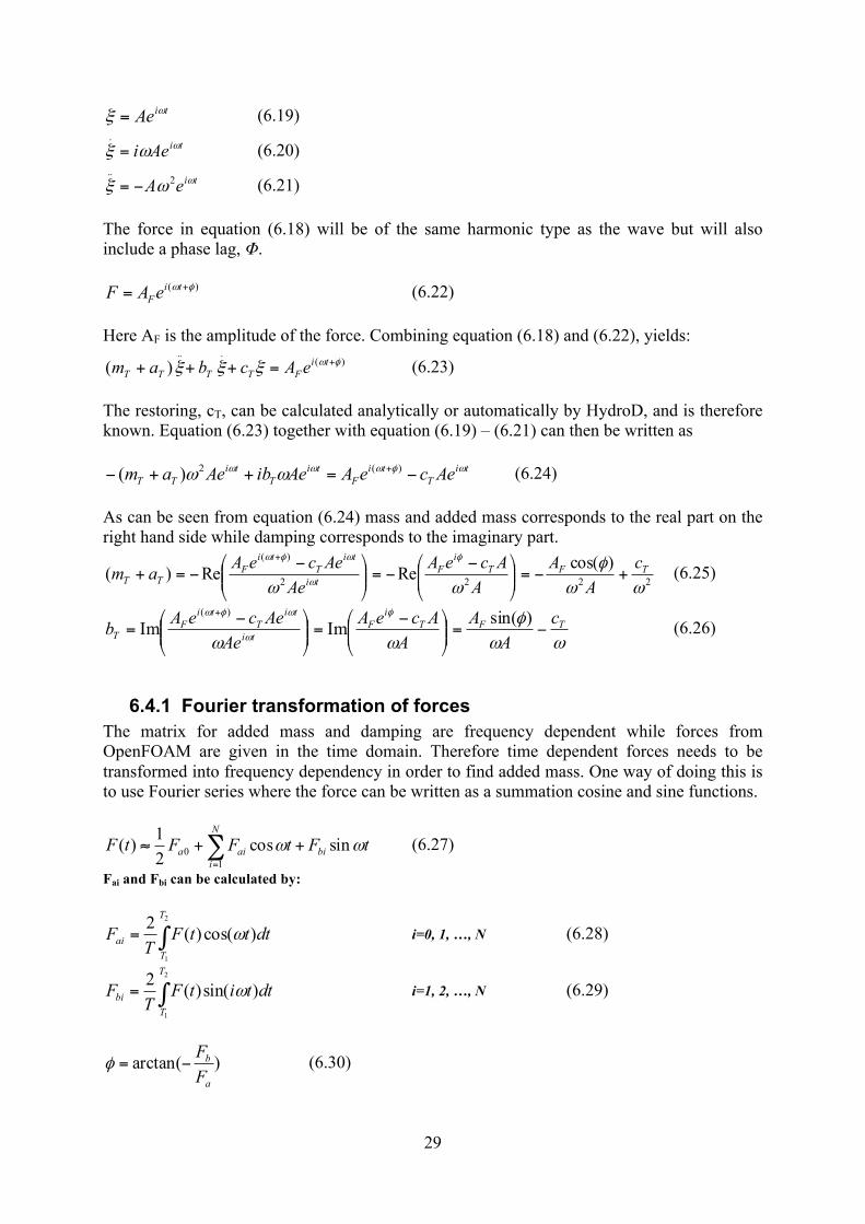
29
tiAe ωξ = (6.19)
tiAei ωωξ =.
(6.20)
tieA ωωξ 2..
−= (6.21) The force in equation (6.18) will be of the same harmonic type as the wave but will also include a phase lag, Φ.
)( φω += tiFeAF (6.22)
Here AF is the amplitude of the force. Combining equation (6.18) and (6.22), yields:
)(...
)( φωξξξ +=+++ tiFTTTT eAcbam (6.23)
The restoring, cT, can be calculated analytically or automatically by HydroD, and is therefore known. Equation (6.23) together with equation (6.19) – (6.21) can then be written as
tiT
tiF
tiT
tiTT AeceAAeibAeam ωφωωω ωω −=++− + )(2)( (6.24)
As can be seen from equation (6.24) mass and added mass corresponds to the real part on the right hand side while damping corresponds to the imaginary part.
2222
)( )cos(ReRe)(
ωωφ
ωω
φ
ω
ωφωTFT
iF
ti
tiT
tiF
TTc
AA
AAceA
AeAeceAam +−=$$
%
&''(
) −−=$$
%
&''(
) −−=+
+
(6.25)
ωωφ
ωω
φ
ω
ωφωTFT
iF
ti
tiT
tiF
Tc
AA
AAceA
AeAeceAb −=$$
%
&''(
) −=$$
%
&''(
) −=
+ )sin(ImIm)(
(6.26)
6.4.1 Fourier transformation of forces The matrix for added mass and damping are frequency dependent while forces from OpenFOAM are given in the time domain. Therefore time dependent forces needs to be transformed into frequency dependency in order to find added mass. One way of doing this is to use Fourier series where the force can be written as a summation cosine and sine functions.
∑=
++≈N
ibiaia tFtFFtF
10 sincos
21
)( ωω (6.27)
Fai and Fbi can be calculated by:
∫=2
1
)cos()(2 T
Tai dtttF
TF ω i=0, 1, …, N (6.28)
∫=2
1
)sin()(2 T
Tbi dttitF
TF ω i=1, 2, …, N (6.29)
)arctan(a
b
FF
−=φ (6.30)

30
7 Validation In this chapter, obtained results for coupling with an open and a closed tank respectively are presented.
7.1 Closed Tank Figure 7.1 shows the comparison between the experimental results from Molin (2002/2008), results from an initial run in HydroD without coupling and then also coupled results. After coupling, the peak seemed to have shifted to the left and a bit higher, named “converged” in figure 7.1. This result converged reasonably quick as described in chapter 7.1.1. After the validation, it was realized that the script, handling the data transformation between the softwares, was not completely correct. Although, it should be mentioned that previously shown results are all recalculated with the correct scripts. With the new script the peak had the same magnitude but was shifted to the right compared to the initial one.
Roll RAO - closed tank
0.00
0.50
1.00
1.50
2.00
2.50
3.00
3.50
4.00
3.00 4.00 5.00 6.00 7.00 8.00Frequency [rad/s]
Am
plitu
de [r
ad/m
]
ExperimentWasim - InitialConvergedNew Script
Figure 7.1: Roll RAO for the closed tank coupling in time domain.
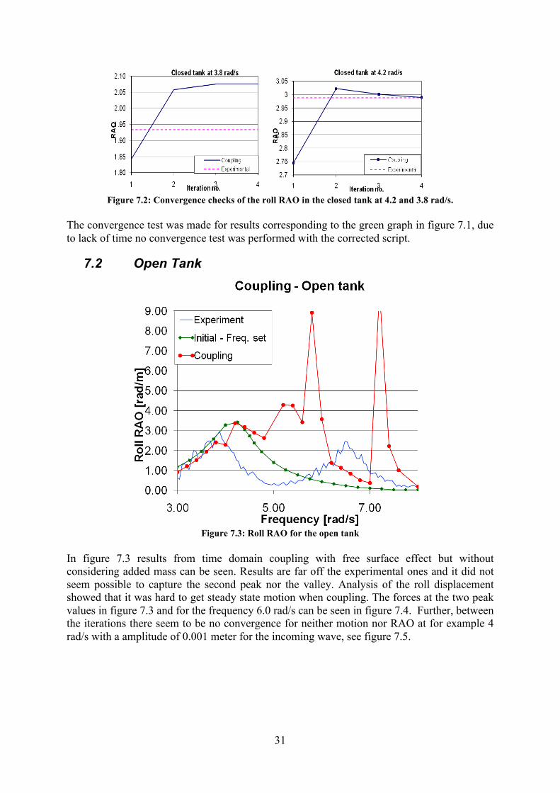
7.1.1 Convergence for Closed Tank Coupling A convergence test for the roll RAO at different frequencies showed that already after one coupling the result seemed to converge, see figure 7.2 where result from two different frequencies are shown. Iteration one in the figures corresponds to the initial run. Since the roll RAO for the initial run can be changed, by changing the additional damping and restoring, it is not proper to use the experimental result as indicator for whether the converged result is correct or not. Before such conclusions can be made simulations with other initial RAO needs to be performed. Although, since converged results are obtained, this gives a good indication since convergence is important.
31
Figure 7.2: Convergence checks of the roll RAO in the closed tank at 4.2 and 3.8 rad/s.
The convergence test was made for results corresponding to the green graph in figure 7.1, due to lack of time no convergence test was performed with the corrected script.
7.2 Open Tank
Figure 7.3: Roll RAO for the open tank
In figure 7.3 results from time domain coupling with free surface effect but without considering added mass can be seen. Results are far off the experimental ones and it did not seem possible to capture the second peak nor the valley. Analysis of the roll displacement showed that it was hard to get steady state motion when coupling. The forces at the two peak values in figure 7.3 and for the frequency 6.0 rad/s can be seen in figure 7.4. Further, between the iterations there seem to be no convergence for neither motion nor RAO at for example 4 rad/s with a amplitude of 0.001 meter for the incoming wave, see figure 7.5.

32
Figure 7.4: Forces from OpenFOAM at 5.8, 6.0 and 7.4 rad/s.
Figure 7.5: Convergence check for the roll RAO in the open tank at 4.0 rad/s
Figure 7.6 shows a comparison between the total force calculated at 4.8 rad/s in HydroD after the initial run and the force from OpenFOAM that was used as auxiliary force for the first coupling. At this frequency the roll RAO is close to zero in the experimental results. The forces in the figure are completely out of phase and the sum of them is close to zero. When coupling the open tank at this frequency, it was expected that the motion would be quite small after the first coupling. Although, the roll RAO showed a higher value than for the initial simulation. This was probably because, when the auxiliary force is sent back to HydroD, it will change the motion of the barge which means that the auxiliary force is not contra acting the current motion.

33
Figure 7.6: Roll moment from the initial computation in HydroD and the auxiliary force that is computed in OpenFOAM based on the corresponding initial motion. The auxiliary force is given back to HydroD for the next iteration.
7.3 Added mass and damping for the tank Wasim provides the user with Fourier transformation automatically when simulating in time domain. By sending forces from OpenFOAM into the Fourier transformer, mass, added mass and damping coefficients can be calculated. In order to validate whether calculating the added mass from the forces would give more satisfactory results, RAO at four frequencies was evaluated; 5.0 rad/s, 5.6 rad/s, 6.0 rad/s and 6.5 rad/s. These frequencies would capture the second peak roll RAO diagram when an open tank was simulated. Table 7.1 gives an overview of the mass (M+A) and damping coefficients, calculated with the so called “Wasim Fourier” feature for the closed tank. Table 7.1
Frequency 5.00 5.60 6.00 6.50
(M+A)22 116.00 114.00 116.00 115.00 (M+A)24 -39.00 -38.10 -39.00 -38.60 (M+A)42 -38.80 -37.90 -38.80 -38.40 (M+A)44 17.50 17.90 17.50 17.30 B22 28.50 44.80 44.30 46.20 B24 -9.58 -16.30 -14.90 -15.60 B42 -9.58 -16.00 -14.90 -15.50 B44 4.43 3.11 6.92 7.18 It was expected that added mass for the closed tank to be relatively small, compared to the mass. The mass of the water inside the tank, corresponding to (M+A)22, was 116 kg. Mass moment of inertia around the global origin, corresponding to (M+A)44, was about 20 Nm, according to analytical calculations for a solid body.

34
In table 7.2 mass (M+A) and damping coefficients for the open tank case are listed. Table 7.2 Frequency
5.00 5.60 6.00 6.50 (M+A)22 -144.00 -223.00 -167.00 -140.00 (M+A)24 -200.00 -116.00 225.00 80.00 (M+A)42 92.50 127.00 92.90 78.60 (M+A)44 116.00 70.00 -113.00 -27.10 B22 1170.00 941.00 238.00 313.00 B24 -298.00 -11500.00 -886.00 51.80 B42 -674.00 -498.00 -108.00 -172.00 B44 159.00 6140.00 472.00 -27.60 For this case it was harder to predict reasonable values for the added mass. Although, observations by Bunnik (2010) showed that added mass due to roll goes to positive and negative infinity at frequencies around the first sloshing mode which is at 5.6 rad/s. Figure 7.7 shows the time history of the forces calculated by OpenFOAM.
Figure 7.7: Force time history in OpenFOAM for 5.0, 5.6, 6.0 and 6.5 rad/s.
Wasim Fourier uses the last time period to calculate added mass and damping. From figure 7.7 it can be seen that using the last time period will not give a true value of the added mass and damping. However, these forces obtained seem reasonable since being close the eigenfrequency of the tank introduces a resonant behavior where the amplitude grows, see figure 7.7. The time period for the force at the frequency close to the eigenfrequency will also be affected.

35
In figure 7.8 results are shown from when the added mass and damping of the tank, for frequencies around where the second peak is located, has been calculated and used in a postprocessor called Waqum Explorer. From this it was possible to get a second peak. In figure 7.9 the influence from changing the restoring force in roll C44, can be seen. The actual restoring was not calculated due to lack of time. Its influence on the peak is rather significant as can be seen below. The quality of the results will be discussed in chapter 8.
Figure 7.8: Roll RAO at the frequencies defining the second peak, where restoring C44 has not been changed
Figure 7.9: Roll RAO at the frequencies defining the second peak, where restoring C44 has been changed to a guessed value.

36
8 Discussion and Conclusion The time domain coupling with a closed tank showed satisfactory results. The peak was shifted a little bit to the right which may be due to dynamic effects that are captured in OpenFOAM but not possible to capture in HydroD. It was noticed that the moment of inertia for the tank was smaller when calculated in OpenFOAM, compared to analytical calculations for a solid body. This seems reasonable since a smaller moment of inertia means a resonant motion at a higher frequency, as according to equation (8.1).
4444
44
AIC+
=ω (8.1)
When introducing the free surface, i.e. simulating with an open tank, some difficulties were introduced into the calculations. It was shown in figure 7.6 that the forces from OpenFOAM were contra acting the forces in HydroD at the given frequency. Although, the results after coupling with an open tank were not as expected. When a large auxiliary force was sent to HydroD, the motions of the barge will be changed, therefore the forces may not be contra acting during the simulation. This could be one explanation for the unexpected result. The trial with added mass, made in the frequency domain, was not as satisfactory as hoped for, but gave an indication that it may be possible to capture the second peak properly by finding the added mass, damping and restoring from the tank. The “correct” peak was not found but at least some sort of second peak was shown to exist around the frequency in question. The captured second peak in figure 7.8 was located between 5.6 and 6.6 rad/s with a magnitude of about 2 rad/m. This can be compared to figure 5.1 where the experimental one was located between approximately 5.6 and 7.5 rad/s and was about 2.5 rad/m in magnitude. Before further conclusions can be made, longer time history for the force needs to be achieved in order to distinguish the force amplitude corresponding to the incoming wave frequency. This can be done by letting Wasim Fourier filter the force amplitude giving the unaffected force amplitude corresponding to the added mass and damping at the specific incoming wave frequency.
8.1 Sources of error Sources of error that could have contributed to results being far off from the experimental ones, are for instance that the mesh size in either OpenFOAM or HydroD was too coarse. This is not the most probable reason for the failure since mesh convergence check was made where the size proved to be fine enough for its purpose. But of course there is always a small influence on the results from grid size, but in this case it is believed that this influence is very small. Using 2D instead of 3D, introduces a similar source of error. A comparison was made which showed some differences. Although, the 2D model was judged to be good enough for its purpose, even though it may have affected the results to some extent. Also, the scripts handling output and input data in between the two programs could have been possible sources of error. These were checked quite a few times and were therefore most probably correct. Another possible source of error was the influence from running single frequencies rather than the whole JONSWAP spectra. Although, this can be dispatched since it was possible to obtain quite accurate results for the closed tank with single frequency. So the actual problem is most likely related to HydroD having difficulties handling the dynamics of the tank. One probable reason why the results from coupling with free surface effect did not come out very well, could be that it was hard to make two programs really communicate without exchanging data for every time step which is called a full coupling. If the problem would have been fully

37
coupled maybe the problem visualized in figure 7.6 with contra acting forces could have been solved. Also, when giving HydroD such big forces as for the open tank case, it is possible that these could have been better handled if a relaxation factor would have been used. In this way, HydroD would have for each iteration, gradually received more and more of the auxiliary force, giving a more stable solution.
8.2 Recommendations The main difference between the closed and open tank case is that centre of gravity will change in an open tank, even in a body-fixed coordinate system. Also, the forces from the tank will be considerably larger if the tank is open. Since the coupling has shown to give reasonable results for closed tank, when forces are smaller, it could be interesting to try to give smaller forces back to Wasim, use a so called relaxation factor, and increase it until the total force from OpenFOAM is accounted for. The number of simulations will then increase but hopefully the result will improve. Also the investigation on finding added mass and damping is worth to proceed with. Since added mass and damping is dependent on frequency only, as described in chapter 6.4.1, only one simulation at each frequency is needed and these results can be used for simulations in other conditions which is convenient. The entire force from OpenFOAM cannot be expressed as added mass, damping and restoring so there will still be some forces to give back to HydroD as an auxiliary force. In this way, hopefully the magnitude of the auxiliary force would be small enough for HydroD to handle.

38
References Andersson, B. Andersson, R. Håkansson, L. Mortensson, M. Sudiyo, R. van Wachem, B. (2010) Computational Fluide Dynamics for Chemical Engineers. Gothenburg, Sweden. Benedict, K. Baldauf, M. Kirchhoff, M. Wismar, H. Estimating Potential Danger of Roll Resonance for Ship Operation. Bergdahl, L. (2010) Wave-Induced Loads and Ship Motions. Gothenburg: Department of Civil and Environmental Engineering. Bunnik, T. Veldman, A. (2010) Modelling the Effects of Sloshing on Ship Motions. Shanghai, China: Proceedings of the ASME 2010 29th International Conference on Ocean, Offshore and Artic Engineering, Dai, Y. (1998) Potential Flow Theory of Ship Motions in Waves in Frequency and Time Domain. Janson, C-E. (2008) Computational Hydrodynamics and Optimization, MMA 160, Potential-flow. Gothenburg: Department of Shipping and Marine Technology. Jasak, H. (1996) Error Analysis and Estimation for the Finite Volume Method with Applications to Fluid Flows. London: Imperial College of Science, Technology & Medicine (PhD Diploma at department of Mechanical Engineering). Kurultay, A A. (2003) SENSITIVITY( ANALYSIS( OF( THE( SEAKEEPING( BEHAVIOR( OF(TRIMARAN( SHIPS.( Monterey:( Naval Postgraduate School Monterey. (M.Sc Thesis at Department of Mechanical and Astronautical Engineering) Molin, B et al. (2002) LNG-FPSO’s: frequency domain, coupled analysis of support and liquid cargo motion. Rethymnon, Greece: Proceedings of the IMAM Conference. Molin, B. Remy, F. Ledoux, A. Ruiz, N. (2008) Effect of roof impacts on coupling between wave response and sloshing in tanks of LNG-carriers. Lisbon, Protugal: proceedings of the 27th International Conference on Offshore Mechanics and Artic Engineering. Pan, Zhi Yuan. (2010) Note on the motion control system in Wasim. Internal technical note, Det Norske Veritas. Pan, Zhi Yuan. (2009) Note on coordinate systems and motions in Wasim. Internal technical not, Det Norske Veritas. Rusche, H. (2002) Computational Fluid Dynamics of Dispersed Two-Phase Flow at high phase fractions. London: Imperial College of Science, Technology & Medicine (PhD Diploma at department of Mechanical Engineering).

39
Appendix A - Code from OpenFOAM® For the simulations in OpenFOAM, a tutorial example of the sloshing tank was used with some modifications. All modifications are shown below where the code from the files in question is listed. These files are BlockMeshDict, BlockMeshDict.m4, controlDict, TransportProperties, fvSchemes, DynamicMeshDict and setFiledsDict. BlockMeshDict FoamFile { version 2.0; format ascii; class dictionary; object blockMeshDict; } // * * * * * * * * * * * * * * * * * * * * * * * * * * * * * * * * * * * * * // // General m4 macros // * * * * * * * * * * * * * * * * * * * * * * * * * * * * * * * * * * * * * // // User-defined parameters convertToMeters 0.01; // Length of tank (x-direction) // Breadth of tank (y-direction) // Depth of tank (z-direction) // Depth to the top (height) of lower chamfer // Height of upper chamfer // Angle of lower chamfer to the horizontal // Angle of upper chamfer to the horizontal // Centre of gravity in y-direction // Centre of gravity in z-direction // Number of cells in the length (1 for 2D) // Number of cells in the breadth // Number of cells in the height of the lower champfer // Number of cells in the height between the chamfers // Number of cells in the height of the upper champfer // * * * * * * * * * * * * * * * * * * * * * * * * * * * * * * * * * * * * * // // Derived parameters // Breadth to the top (height) of lower chamfer // Breadth of upper chamfer // * * * * * * * * * * * * * * * * * * * * * * * * * * * * * * * * * * * * * //

40
// Parametric description vertices( (-0.5 -40 -5.242223942) // Vertex bllcb = 0 (-0.5 -40 -5.242223942) // Vertex bllc = 1 (-0.5 -40 23.757776058) // Vertex bluc = 2 (-0.5 -40 23.757776058) // Vertex bluct = 3 (-0.5 40 -5.242223942) // Vertex brlcb = 4 (-0.5 40 -5.242223942) // Vertex brlc = 5 (-0.5 40 23.757776058) // Vertex bruc = 6 (-0.5 40 23.757776058) // Vertex bruct = 7 (0.5 -40 -5.242223942) // Vertex fllcb = 8 (0.5 -40 -5.242223942) // Vertex fllc = 9 (0.5 -40 23.757776058) // Vertex fluc = 10 (0.5 -40 23.757776058) // Vertex fluct = 11 (0.5 40 -5.242223942) // Vertex frlcb = 12 (0.5 40 -5.242223942) // Vertex frlc = 13 (0.5 40 23.757776058) // Vertex fruc = 14 (0.5 40 23.757776058) // Vertex fruct = 15 ); blocks ( // block0 hex (0 4 5 1 8 12 13 9) (80 0 1) simpleGrading (1 1 1) // block1 hex (1 5 6 2 9 13 14 10) (80 29 1) simpleGrading (1 1 1) // block2 hex (2 6 7 3 10 14 15 11) (80 0 1) simpleGrading (1 1 1) ); patches ( patch walls ( (0 4 12 8) (4 5 13 12) (5 6 14 13) (6 7 15 14) (7 3 11 15) (3 2 10 11)

41
(2 1 9 10) (1 0 8 9) ) empty front ( (8 12 13 9) (9 13 14 10) (10 14 15 11) ) empty back ( (0 1 5 4) (1 2 6 5) (2 3 7 6) ) ); // ************************************************************************* // BlockMeshDict.m4 FoamFile { version 2.0; `format' ascii; class dictionary; object blockMeshDict; } // * * * * * * * * * * * * * * * * * * * * * * * * * * * * * * * * * * * * * // // General m4 macros. changecom(//)changequote([,]) dnl> define(calc, [esyscmd(perl -e 'use Math::Trig; print ($1)')]) dnl> define(VCOUNT, 0) define(vlabel, [[// ]Vertex $1 = VCOUNT define($1, VCOUNT)define([VCOUNT], incr(VCOUNT))]) define(hex2D, hex (b$1 b$2 b$3 b$4 f$1 f$2 f$3 f$4)) define(quad2D, (b$1 b$2 f$2 f$1)) define(frontQuad, (f$1 f$2 f$3 f$4)) define(backQuad, (b$1 b$4 b$3 b$2)) // * * * * * * * * * * * * * * * * * * * * * * * * * * * * * * * * * * * * * // // User-defined parameters convertToMeters 0.01; define(l, 1) // Length of tank (x-direction)

42
define(b, 80) // Breadth of tank (y-direction) define(h, 29) // Depth of tank (z-direction) define(hlc, 0) // Depth to the top (height) of lower chamfer define(huc, 0) // Height of upper chamfer define(thetalc, 90) // Angle of lower chamfer to the horizontal define(thetauc, 90) // Angle of upper chamfer to the horizontal define(CofGy, calc(b/2.0)) // Centre of gravity in y-direction define(CofGz, 5.242223942) // Centre of gravity in z-direction define(Nl, 1) // Number of cells in the length (1 for 2D) define(Nb, 80) // Number of cells in the breadth define(Nhlc, 0) // Number of cells in the height of the lower champfer define(Nh, 29) // Number of cells in the height between the chamfers define(Nhuc, 0) // Number of cells in the height of the upper champfer // * * * * * * * * * * * * * * * * * * * * * * * * * * * * * * * * * * * * * // // Derived parameters define(blc, calc(hlc/tan(deg2rad(thetalc)))) // Breadth to the top (height) of lower chamfer define(buc, calc(huc/tan(deg2rad(thetauc)))) // Breadth of upper chamfer define(Yl, -CofGy) define(Yllc, calc(Yl + blc)) define(Yluc, calc(Yl + buc)) define(Yr, calc(Yl + b)) define(Yrlc, calc(Yr - blc)) define(Yruc, calc(Yr - buc)) define(Zb, -CofGz) define(Zlc, calc(Zb + hlc)) define(Zt, calc(Zb + h)) define(Zuc, calc(Zt - huc)) define(Xf, calc(l/2.0)) define(Xb, calc(Xf - l)) // * * * * * * * * * * * * * * * * * * * * * * * * * * * * * * * * * * * * * // // Parametric description vertices ( (Xb Yllc Zb) vlabel(bllcb) (Xb Yl Zlc) vlabel(bllc) (Xb Yl Zuc) vlabel(bluc) (Xb Yluc Zt) vlabel(bluct) (Xb Yrlc Zb) vlabel(brlcb)

43
(Xb Yr Zlc) vlabel(brlc) (Xb Yr Zuc) vlabel(bruc) (Xb Yruc Zt) vlabel(bruct) (Xf Yllc Zb) vlabel(fllcb) (Xf Yl Zlc) vlabel(fllc) (Xf Yl Zuc) vlabel(fluc) (Xf Yluc Zt) vlabel(fluct) (Xf Yrlc Zb) vlabel(frlcb) (Xf Yr Zlc) vlabel(frlc) (Xf Yr Zuc) vlabel(fruc) (Xf Yruc Zt) vlabel(fruct) ); blocks ( // block0 hex2D(llcb, rlcb, rlc, llc) (Nb Nhlc Nl) simpleGrading (1 1 1) // block1 hex2D(llc, rlc, ruc, luc) (Nb Nh Nl) simpleGrading (1 1 1) // block2 hex2D(luc, ruc, ruct, luct) (Nb Nhuc Nl) simpleGrading (1 1 1) ); patches ( patch walls ( quad2D(llcb, rlcb) quad2D(rlcb, rlc) quad2D(rlc, ruc) quad2D(ruc, ruct) quad2D(ruct, luct) quad2D(luct, luc) quad2D(luc, llc) quad2D(llc, llcb) ) empty front ( frontQuad(llcb, rlcb, rlc, llc) frontQuad(llc, rlc, ruc, luc)

44
frontQuad(luc, ruc, ruct, luct) ) empty back ( backQuad(llcb, rlcb, rlc, llc) backQuad(llc, rlc, ruc, luc) backQuad(luc, ruc, ruct, luct) ) ); DynamicMeshDict FoamFile { version 2.0; format ascii; class dictionary; location "constant"; object dynamicMeshDict; } // * * * * * * * * * * * * * * * * * * * * * * * * * * * * * * * * * * * * * // dynamicFvMesh solidBodyMotionFvMesh; solidBodyMotionFvMeshCoeffs { solidBodyMotionFunction SKA; SKACoeffs { CofG ( 0 0 0 ); timeDataFileName "constant/80.dat"; } } // ************************************************************************* // TransportProperties FoamFile { version 2.0; format ascii; class dictionary; location "constant"; object transportProperties;
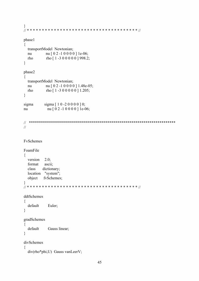
45
} // * * * * * * * * * * * * * * * * * * * * * * * * * * * * * * * * * * * * * // phase1 { transportModel Newtonian; nu nu [ 0 2 -1 0 0 0 0 ] 1e-06; rho rho [ 1 -3 0 0 0 0 0 ] 998.2; } phase2 { transportModel Newtonian; nu nu [ 0 2 -1 0 0 0 0 ] 1.48e-05; rho rho [ 1 -3 0 0 0 0 0 ] 1.205; } sigma sigma [ 1 0 -2 0 0 0 0 ] 0; nu nu [ 0 2 -1 0 0 0 0 ] 1e-06; // ************************************************************************* // FvSchemes FoamFile { version 2.0; format ascii; class dictionary; location "system"; object fvSchemes; } // * * * * * * * * * * * * * * * * * * * * * * * * * * * * * * * * * * * * * // ddtSchemes { default Euler; } gradSchemes { default Gauss linear; } divSchemes { div(rho*phi,U) Gauss vanLeerV;

46
div(phi,alpha) Gauss vanLeer; div(phirb,alpha) Gauss vanLeer; } laplacianSchemes { default Gauss linear corrected; } interpolationSchemes { default linear; } snGradSchemes { default corrected; } fluxRequired { default no; p; pcorr; alpha; } // ************************************************************************* // controlDict FoamFile { version 2.0; format ascii; class dictionary; location "system"; object controlDict; } // * * * * * * * * * * * * * * * * * * * * * * * * * * * * * * * * * * * * * // application interDyMFoam; startFrom startTime; startTime 0; stopAt endTime;

47
endTime 30; deltaT 0.01; writeControl adjustableRunTime; writeInterval 0.01; purgeWrite 0; writeFormat ascii; writePrecision 6; writeCompression compressed; timeFormat general; timePrecision 6; runTimeModifiable yes; adjustTimeStep yes; maxCo 0.5; maxDeltaT 1; functions { probes { type probes; functionObjectLibs ("libsampling.so"); outputControl timeStep; outputInterval 1; probeLocations ( ( 0 9.95 19.77 ) ( 0 -9.95 19.77 ) ); fields ( p ); } wallPressure {

48
type surfaces; functionObjectLibs ("libsampling.so"); outputControl timeStep; outputInterval 10; surfaceFormat raw; fields ( p ); surfaces ( walls { type patch; patchName walls; triangulate false; } ); } forces //forces { type forces; functionObjectLibs ("libforces.so"); outputControl outputTime; outputInterval 1; patches (walls); rhoInf 998.0; CofR (0 0 0); } } // ************************************************************************* // setFieldsDict FoamFile { version 2.0; format ascii; class dictionary; location "system"; object setFieldsDict; } // * * * * * * * * * * * * * * * * * * * * * * * * * * * * * * * * * * * * * // defaultFieldValues
49
( volScalarFieldValue alpha1 0 //air phase ); regions ( boxToCell { box ( -100 -100 -100 ) ( 100 100 0.237578); //coords of rectangular prism containing liquid fieldValues ( volScalarFieldValue alpha1 1 //liquid phase ); } ); // ************************************************************************* //

50
Appendix B - Code from Scripts The files all.py, forcesOF.py, fromOF.py and motionandacc.py were used to process the forces from openFOAM. motionmodifier.py was used to process the motion input to OpenFOAM. all.py print 'Starting forcesOF' import forcesOF print 'starting motionandacc' import motionandacc print 'starting fromOF' import fromOF forcesOF.py import xlrd import sys import glob import xlwt import xlutils import csv from xlrd import open_workbook,cellname ##book1 = open_workbook('first_motion_2.xls') ##sheet = book1.sheet_by_index(0) ##print sheet.name ##print sheet.nrows ##print sheet.ncols from tempfile import TemporaryFile from xlwt import Workbook, Formula book2=Workbook() Sheet1 = book2.add_sheet('Sheet 1',cell_overwrite_ok=True) # open file to read f = file('forces.dat', 'r') d=0 # iterate over the lines in the file for line in f: columns =map(str,line.split())

51
columns = [col.strip('() ') for col in columns] # ensure the column has at least one value before printing if d<=0: Sheet1.row(d).write(1,columns[1]) elif d>0: Sheet1.row(d).set_cell_number(0,columns[0]) Sheet1.row(d).set_cell_number(4,columns[1]) Sheet1.row(d).set_cell_number(5,columns[2]) Sheet1.row(d).set_cell_number(6,columns[3]) Sheet1.row(d).set_cell_number(9,columns[4]) Sheet1.row(d).set_cell_number(10,columns[5]) Sheet1.row(d).set_cell_number(11,columns[6]) Sheet1.row(d).set_cell_number(16,columns[7]) Sheet1.row(d).set_cell_number(17,columns[8]) Sheet1.row(d).set_cell_number(18,columns[9]) Sheet1.row(d).set_cell_number(21,columns[10]) Sheet1.row(d).set_cell_number(22,columns[11]) Sheet1.row(d).set_cell_number(23,columns[12]) d=d+1 print 'forces.xls created' book2.save('forces.xls') fromOF.py import xlrd import sys import glob import xlwt import xlutils import csv from xlrd import open_workbook,cellname ##book1 = open_workbook('first_motion_2.xls') ##sheet = book1.sheet_by_index(0) ##print sheet.name ##print sheet.nrows ##print sheet.ncols from tempfile import TemporaryFile from xlwt import Workbook, Formula book2=Workbook() Sheet1 = book2.add_sheet('Sheet 1',cell_overwrite_ok=True) # open file to read f = file('forces.dat', 'r') d=0

52
# iterate over the lines in the file for line in f: columns =map(str,line.split()) columns = [col.strip('() ') for col in columns] # ensure the column has at least one value before printing if d<=0: Sheet1.row(d).write(1,columns[1]) elif d>0: Sheet1.row(d).set_cell_number(0,columns[0]) Sheet1.row(d).set_cell_number(4,columns[1]) Sheet1.row(d).set_cell_number(5,columns[2]) Sheet1.row(d).set_cell_number(6,columns[3]) Sheet1.row(d).set_cell_number(9,columns[4]) Sheet1.row(d).set_cell_number(10,columns[5]) Sheet1.row(d).set_cell_number(11,columns[6]) Sheet1.row(d).set_cell_number(16,columns[7]) Sheet1.row(d).set_cell_number(17,columns[8]) Sheet1.row(d).set_cell_number(18,columns[9]) Sheet1.row(d).set_cell_number(21,columns[10]) Sheet1.row(d).set_cell_number(22,columns[11]) Sheet1.row(d).set_cell_number(23,columns[12]) d=d+1 print 'forces.xls created' book2.save('forces.xls') motionandacc.py import xlrd import sys import glob import xlwt import xlutils import csv from tempfile import TemporaryFile from xlwt import Workbook, Formula #Open File to write to book2=Workbook() Sheet1 = book2.add_sheet('Sheet 1',cell_overwrite_ok=True) book1=Workbook() Sheet2 = book1.add_sheet('Sheet 1',cell_overwrite_ok=True) book3=Workbook() Sheet3 = book3.add_sheet('Sheet 1',cell_overwrite_ok=True)

53
# open file to read f = file('WasimActivityFSEInitial78_Run1.mot_acc', 'r') f2 = file('WasimActivityFSEInitial78_Run1.mot', 'r') f3 = file('WasimActivityFSEInitial78_Run1.mot_vel', 'r') d=0 for line in f: columns2 =map(str,line.split()) if d>=3: Sheet1.row(d-2).set_cell_number(0,columns2[0]) Sheet1.row(d-2).set_cell_number(1,columns2[2]) Sheet1.row(d-2).set_cell_number(2,columns2[3]) Sheet1.row(d-2).set_cell_number(3,columns2[4]) d=d+1 print 'acc.xls file created' book2.save('acc.xls') d=0 for line in f2: columns3 =map(str,line.split()) if d>=3: Sheet2.row(d-2).set_cell_number(0,columns3[0]) Sheet2.row(d-2).set_cell_number(1,columns3[2]) Sheet2.row(d-2).set_cell_number(2,columns3[3]) Sheet2.row(d-2).set_cell_number(3,columns3[4]) d=d+1 print 'mot.xls file created' book1.save('mot.xls') d=0 for line in f3: columns4 =map(str,line.split()) if d>=3: Sheet3.row(d-2).set_cell_number(0,columns4[0]) Sheet3.row(d-2).set_cell_number(1,columns4[2]) Sheet3.row(d-2).set_cell_number(2,columns4[3]) Sheet3.row(d-2).set_cell_number(3,columns4[4]) d=d+1 print 'vel.xls file created' book3.save('vel.xls') motionModifier.py __author__ = "jackie" __version__ = "$Revision: 1.2 $" __date__ = "$Date: 2011/03/28 21:57:19 $" __copyright__ = "Copyright (c) 2001 Mark Pilgrim" __license__ = "Python"
54
inFile= file('WasimActivityFSEInitial78_Run1.mot','r') outFile=file('motionInput.dat','w') lines=inFile.readlines() nbrLines=sum([1 for line in lines]) lines2='' for line in lines[3:]: columns=map(str, line.split()) lines2=lines2+'('+str(columns[0])+' (('+str(columns[1])+' '+ str(columns[2])+' '+str(columns[3])+' )( '+str(columns[4])+' '+str(columns[5])+' '+str(columns[6])+' )))\n' outFile.write('(\n') outFile.writelines(lines2) outFile.write('\n )') outFile.write(')')

55
Appendix C – Drawing