capturing heat transfer for complex-shaped multibody

Computational Particle Mechanics (2020) 7:919–934https://doi.org/10.1007/s40571-020-00321-w

Capturing heat transfer for complex-shapedmultibody contactproblems, a new FDEM approach

Clément Joulin1 · Jiansheng Xiang1 · John-Paul Latham1 · Christopher Pain1 · Pablo Salinas1

Received: 21 June 2019 / Revised: 10 February 2020 / Accepted: 12 February 2020 / Published online: 22 February 2020© The Author(s) 2020

AbstractThis paper presents a new approach for the modelling of heat transfer in 3D discrete particle systems. Using a combinedfinite–discrete element (FDEM) method, the surface of contact is numerically computed when two discrete meshes of twosolids experience a small overlap. Incoming heat flux and heat conduction inside and between solid bodies are linked.In traditional FEM (finite element method) or DEM (discrete element method) approaches, to model heat transfer acrosscontacting bodies, the surface of contact is not directly reconstructed. The approach adopted here uses the number of surfaceelements from the penetrating boundary meshes to form a polygon of the intersection, resulting in a significant decrease inthe mesh dependency of the method. Moreover, this new method is suitable for any sizes or shapes making up the particlesystem, and heat distribution across particles is an inherent feature of the model. This FDEM approach is validated againsttwo models: a FEM model and a DEM pipe network model. In addition, a multi-particle heat transfer contact problem ofcomplex-shaped particles is presented.

Keywords Contact heat transfer · Finite element method, FEM · Discrete element method, DEM · Finite–discrete elementmethod, FDEM · Heat resistance · Explicit method · Implicit method

1 Introduction

Heat transfer in particle systems is encountered in a largenumber of applications such as chemical and nuclear engi-neering and in soil and fluid mechanics. Finite elementmethods (FEM) have been used in the modelling of micro-scopic contact roughness and/or mechanical interactions[14,24,27,31]. More advanced work included modelling ofthe contact roughness structure and deformations togetherwith contact heat transfer [22]. However, these works aimto model mechanical and thermal interactions of a specificcontact configuration rather than study of the overall heat dis-tribution across multiple contacting solid bodies. A similarfinite elements procedure has been presented [4,17], usingboundary nodes of the contacting solids to determine heatflow through contact zones. However, the latter method istwo-dimensional and has no intent or ability to model multi-particle systems. The powerful digitalisedmethod from Jia et

B Jiansheng [email protected]

1 Department of Earth Science and Engineering, ImperialCollege London, London, UK

al. in 2002 [16] enabled the use of arbitrary sizes and shapesin 2Dwith the ability to model large systemswith a low com-putational effort; however, the pixelisation of particles andtheir boundaries presents consistent limitations when study-ing contact problems.Discrete element methods (DEM) are specific to the anal-ysis of multi-bodies, relying on a low computational effortand enabling simulations with large sets of particles. Hence,research onmultibody contact heat transfer with discrete ele-ments has been very active in the past 25 years. A large rangeof publications treated as the heat conduction across ran-domly packed spheres, in 1990 Jagota et al. [15], establisheda method to determine the effective thermal conductivity ofa packing of spheres. Following this direction, Argento andBouvard [2] pioneered the use of FEM model for the defor-mation of spheres in contact. Hence, linkage between thecontact area and the heat resistance is important. Cheng et al.modelled heat transfer in mono-sized spheres in the presenceof a stagnant fluid [7]. Siu and Lee [30] presented in 2004 athree-dimensional model for randomly packed spheres. Fenget al. [9,10] developed a pipe network model to simulateheat transfer in large numbers of circular particles in 2Dthat represent infinite or long pipes. Rickelt et al. [25,26]

123

http://crossmark.crossref.org/dialog/?doi=10.1007/s40571-020-00321-w&domain=pdf

920 Computational Particle Mechanics (2020) 7:919–934

developed a radial temperature model that allows to simulategranular systems of particles of different sizes and materi-als, enabling the use of DEM in various applications. Ganet al. [11] extended DEM to simulate contact heat trans-fer in packed and fluidized beds of ellipsoids. However, theabovemethods are restricted to the analysis of simple-shapedparticles (spheres, discs, cylinders, ellipsoids, etc.) in past.Although DEM extends its capabilities to simulate complexshapes using superquadrics [1], polyhedral DEM for convex[13,29] and non-convex particle shapes [12], clustered sphere[8], etc., it still relies on the assumption that the temperatureis uniform within each particle which is not valid in someconfigurations as this present paper will highlight. For morecomplex contact conditions, it is very difficult to provide anaccurate solution using DEM. Finally, to compute the heatdistribution within each particle, DEM models rely, whenavailable, on extra analytical solutions [9,10,25,26]. Schereret al. [28] concluded the best solution might be to use FDEMwhich can be used to describe particle deformation. But tothe best knowledge of the authors, FDEM has not yet beenapplied to thermochemical problems within DEM.This paper presents a new approach for three-dimensionalmultibody contact heat transfer using the FDEM approach[20] where discrete particles are described with FEM meshand interactions between them are treated with the DEMapproach. The contact interactions between discrete bodiesare calculated via the penalty function method [21] relyingon the overlap between the contacting discretemeshes. Usingthis existing algorithm, the presented method evaluates theapparent contact surface area from the contact overlap ofdiscrete meshes. Contact heat flux is calculated from theboundary temperatures of the solids involved in the con-tact. Moreover, this method possesses the advantage of beingsuited to simulating an accumulation of particles of any sizesand shapes for which the heat distribution within a particlemay be an important feature. (This in contrast to DEM butcomes at a higher computational cost.)This paper unfolds as follows: Firstly, the theory of standardheat conduction and contact heat transfer in the FDEM codeis presented in Sect. 2 and 3 and then validated in Sect. 4;secondly, the FDEM contact model is compared to a DEMpipe network contact model [9,10] in Sect. 5. Finally, thecode’s ability to model complex configurations of particlesis demonstrated in Sect. 6.

2 Finite element equations for heat transfer

2.1 Problem Statement—This section presentsmodified equations from [23]

Let us consider an isotropic body with non-temperature-dependent heat transfer properties. A basic equation of heat

transfer has the following form:

−(

∂qx

∂x+ ∂qy

∂ y+ ∂qz

∂z

)+ Q = ρc

∂T

∂t(1)

With qx ,qy,qz components of the heat flow through an unitarea, Q is the inner heat generation rate per unit volume; ρ

is the material density; c is the heat capacitance; T is thetemperature field; and t is time. According to Fourier’s law,the components of the heat flow can be expressed as follows:

qx = −k∂T

∂x, qy = −k

∂T

∂ y, qz = −k

∂T

∂z, (2)

The thermal conductivity coefficient of the media is noted k,and the combination of these equations yield the followingbasic heat transfer equation:

k

(∂2T

∂x2+ ∂2T

∂ y2+ ∂2T

∂z2

)+ Q = ρc

∂T

∂t(3)

We then consider the following boundary conditions:

– The initial temperature T (x, y, z, t = 0) = T0(x, y, z),– Specified temperature or Dirichlet boundary condition

Ts = T (x, y, z, t) on surface boundary Γs ,– Specified heat flux orNeumann boundary conditionqh =

−(qxnx + qyny + qznz) on Γh ,– Contact heat flux qc on contact surface boundary Γc,– Convection boundary condition qcv = h ΔTsolid−env onsurface boundary Γcv . ΔTsolid−env being the temperaturedifference between the solid and the temperature of theenvironment in which the solid is placed, h is the heatconvection coefficient.

2.2 Finite element discretisation

The domain V is divided into finite elements connected atnodes; the boundary of the domain is noted Γ . Interpolationfunctions are used for calculation of temperature inside eachfinite element composed of ne nodes:

T = N{T }�,N = [N1 N2 · · · Nne ], {T } = {T1 T2 · · · Tne }(4)

T is the matrix of temperature distribution inside the finiteelement, {T } is the vector of temperatures at the nodes, andNis the interpolation or shape functionmatrix. In this study, weuse four-noded tetrahedral elements, and the correspondingshape function is:

N1 = ζ1, N2 = ζ2, N3 = ζ3, N4 = ζ4 = 1−ζ1−ζ2−ζ3

(5)

123

Computational Particle Mechanics (2020) 7:919–934 921

With ζne the isoparametric coordinates so that ζ1 + ζ2 + ζ3 +ζ4 = 1. The spatial gradient of the shape function B is:

⎛⎜⎜⎜⎜⎜⎜⎜⎝

∂T∂x

∂T∂ y

∂T∂z

⎞⎟⎟⎟⎟⎟⎟⎟⎠

=

⎡⎢⎢⎢⎢⎢⎢⎢⎣

∂N1∂x

∂N2∂x · · ·

∂N1∂ y

∂N2∂ y · · ·

∂N1∂z

∂N2∂z · · ·

⎤⎥⎥⎥⎥⎥⎥⎥⎦

{T } = B{T } (6)

Similarly to temperature, the source term is declined in nodalvalues:

Q = N{Q}�, {Q} = {Q1 Q2 · · · Qne } (7)

Wehave the following equation for a finite element of volumeV :

∫V

(k∂T∂x

+ k∂T∂ y

+ k∂T∂z

− Q − ρc∂T∂t

)dV = 0 (8)

Applying the finite element discretisation yields:

∫V

[k∇(Bi j Ti ) − Qi Ni − ρc

∂Ti∂t

Ni

]dV = 0 (9)

where i = 1, . . . , ne represent each set of equations in thefinite element. Applying the divergence theorem yields:

∫VBi j B ji Ti dV +

∫Γ

{qi }{ni }� Ni dΓ

= ρc∫V

∂Ti∂t

Ni dV +∫VQi Ni dV (10)

with

{qi } = [qxi q y

i qzi], {ni } = [

nxi nyi nzi]

(11)

where {ni } is an outer normal to the surface of the body. Also,it is worth noting that

{qi } = −k Bi j Ti (12)

After insertion of boundary conditions into Eq. 10 and usingEq. 12, the discretised equations are as follows:

ρc∫V

∂Ti∂t

Ni dV − k∫VBi j B ji Ti dV

= −∫VQi Ni dV +

∫Γh

qhi Ni dΓ

−∫

Γc

qci Ni dΓ −∫

Γcv

qcvi Ni dΓ

(13)

Finally, we obtain the following condensed expression of thefinite element model:

Mi j Ti + Ki j Ti = BQi + Bh

i + Bci + Bcv

i (14)

Mi j = ρc∫V

Ni N j dV (15)

Ki j = k∫V

Bi j B ji dV (16)

BQi = −

∫VQi (x, y, z, t) Ni dV (17)

Bhi =

∫Γh

qhi Ni dΓ (18)

Bci =

∫Γc

qci Ni dΓ (19)

Bcvi =

∫Γcv

qcvi Ni dV

= −∫

Γcv

h ΔTsolid−env Ni dΓ (20)

2.3 Thermal contact

The heat flux across the apparent surface area of two solidsin contact is defined as follows:

qc = ΔTcRc

(21)

in which Rc is the contact heat resistance and ΔTc the appar-ent temperature drop at the contact. This definition introducesa fictional apparent temperature drop at the interface. Inreality, there is no real discontinuity of the temperature dis-tribution through the solids’ contacts. There is a continuousdistribution of temperature extending through the contactinterface from both solids. As shown in Fig. 1, definingthe temperature drop as the difference in the temperatureobtained by extrapolating the temperature profiles in the tworegions of the interface enables the use of the contact heatresistance to simplify the complex heat processes occurringat the boundary.

2.4 Temporal integration

The differential Eq. 14 needs to be integrated with respect totime to obtain a transient solution of the heat equation. Asdefined in [18], the θ -family time integration methods are ofthe most commonly used:

{T }n+1 = {T }n +Δt[(1− θ){T }n + θ{T }n+1], 0 ≤ θ ≤ 1

(22)

123


Fig. 1 Definition of the contact temperature drop, from [19]

The term {T }n is obtained from solving Eq. 14. For θ = 0,we obtain the explicit forward difference scheme:

{T }n+1 = {T }n + Δt {T }n (23)

For different θ > 0, the above equation will refer to mixedimplicit–explicit methods. For θ = 1, we obtain the fullyimplicit backward difference (or backward Euler) methodwhich is unconditionally stable, i.e. there is no restriction onthe time step size. The theta method offers a large range ofoptions for solving steady state and transient contact prob-lems, as the final temperature distribution can be obtained inone iteration (θ = 1), and different transient states can becomputed with accuracy (θ > 0).

3 A new contact heat transfer method

3.1 Contact surface area

The presented method evaluates the contact area betweentwo contacting solids based on the penetration of boundarymeshes, see Fig. 2. This surface calculation method is basedon the routines of the Y code developed by A. Munjiza [20].A contact surface is obtained for both solids, and the over-all contact surface is the average of these two values. Themethod selects a couple of contacting elements, one is calledthe contactor element, and the other one is called the targetelement. The boundary surface of the target element in con-tact with the whole contactor element’s volume is calculated,and then the opposite calculation is performed. Each solid ismeshed with four-noded tetrahedral elements, the algorithmloops on each face of the target element, and the intersectionsurface with the contactor’s volume is drawn on each target’sface (and vice versa), see Fig. 3a.

Fig. 2 Contact overlap between two solids’ boundaries

Two surface areas are obtained, one describing the contactarea on the target, the other on the contactor, which we call,respectively, Star and Scon, the contact area is set to be theaverage of these two. Note that only the faces of the targetelement located on the boundary of the solid can be selectedfor surface calculation. Figure 4 shows boundary elementsfrom a first solid A contacting a boundary element froma second solid B. For purposes of explanation of the sur-face calculation, consider the blue element to be the targetelement and red elements to be selected successively as con-tactor elements; also note that the relative penetration size hasbeen intentionally exaggerated on the figures. Then, considerthat the target element from solid B possesses only one facelocated on the boundary of solid B; this face is highlighted inFig. 3b. The algorithm will intersect this face with all threecontactor element volumes from solid A in order to recon-struct the surface area of contact; therefore, three Starcontactareas are obtained, see Fig. 3c. At last, the opposite calcula-tion is performed, and surfaces Scon are obtained.

3.2 Computation of heat fluxes

Heat fluxes are calculated between each couples of contactingtetrahedral elements from two contacting solids meshes. Thetotal contact heat flux temperature contribution of Eq. 14 isfor a finite element:

Bci =

nc∑k=1

Bc,ki = 1

3RkcΔT k

c Skc (24)

where nc the number of contacts for which node i is involvedin. The contribution is equally distributed between the threesurface nodes of each contacting tetrahedron; hence, we havea 13 factor. S

kc is the contact surface of the k contact, being the

average between the contactor’s and the target’s overlappingboundary surfaces:

123


Fig. 3 Element contact

Skc = 1

2(Sktar + Skcon) (25)

Figure 5 shows the contact heat transfer for two isolated con-tacting tetrahedral elements. The nodal heat flux contributionfor the contacting surfaces (T12, T13, T14) and (T21, T22, T24)is the following for nodes T12, T13 and T14:

Bc1=

1

6Rc

(T12+T13+T14

3− T21 + T22 + T24

3

)(Star+Scon)

(26)

And for nodes T21, T22 and T24:

Bc2 = −Bc

1 (27)

We can summarise themethodwith the following expression:

Bci =

nc∑k=1

1

18Rkc

4∑l=1

(T kcon,l − T k

tar,l) (Sktar + Skcon) (28)

Fig. 4 Element-to-element surface calculation for two contacting solids

where T kcon,l and T k

tar,l the nodal temperatures of the targetand the contactor elements involved in the k contact.

3.3 Contact interactionmatrix

Pursuing the objective of solving large complex contact heattransfer problems in a minimum time, the PETSc tool-kitfor scientific computation is solving the general heat transferdifferential Eq. 14 which was implemented in our program.In order towrite Eq. 28 in amatrix form,we define the contactinteraction term Bc

i as follows:

Bci = Chi j Ti (29)

where Ch is the contact heat transfer interaction [ne; ne]sparsematrix containing node interactions between elements

123


Fig. 5 Nodal temperatures of two overlapping tetrahedral elements

of separate bodies,ne, the total number of nodes of the studiedcontact problem. We can decompose the contact interac-tion matrix into a sum of nc sub-sparse interaction [ne; ne]matrixes:

Chi j =nc∑k=1

1

18RkcCki j (Sktar + Skcon)

Cki j = +1 i f i = j

Cki j = −1 i f i �= j

(30)

where i, j ∈ [1, 2, . . . , ne] nodal indexes of the target andcontactor elements of the considered contact couples.

3.4 Calculation procedure

The presented thermal contact model is integrated into theFDEM framework and follows the following procedure:

1. Contact detection2. Contact interaction

(a) Surface calculation(b) Computation of heat fluxes(c) Construction of the contact interaction matrix

3. Solving of the thermal equation4. Solving for deformation and motion

3.5 Algorithm limitations

This algorithm excels in capturing the surface area of con-tact as the intersection polygon is drawn across the elementsfaces; however, in the event ofmodelling solidswith complexshapes and curves, the surface area calculation can only beas good as the mesh approximation of the solid’s boundary.In addition, the surface of contact is linked to the amountof mesh penetration which depends on the penalty func-tion. Depending on the configuration of the contact (edgeto edge, edge to surface or surface to surface), the penalty

function may or may not influence the surface of contact ina significant manner, and further research on this topic isnecessary. Nevertheless, the method remains conservative;the contact heat flux distribution is bound to be equal andopposite between two solids as the same quantity of heat isexchanged over the same area.

4 FEM and FDEM perfect contact conductionvalidation

In this section, we validate the finite element conduction heattransfer through one continuous solid and the contact heattransfer across two contacting solids with a perfect contact.Results are comparedwith a one-dimensional analytical solu-tion for conduction in solids.

4.1 Analytical solution

Consider a finite slab of length L, the solid is of an initialtemperature of T0. The left side of the slab is insulated, whilethe right side is exposed to a Dirichlet boundary conditionof an imposed temperature TD, see Fig. 6. There is no innerheat generation in the slab. The one-dimensional transientconduction equation for this problem is:

∂2T

∂x2= 1

α

∂T

∂t, α = c

k(31)

where α the thermal diffusivity, k the thermal conductivityand c the thermal capacity. The solution given in [5] is of theform:

θ =∞∑n=1

4 sin(n − π/2)

2(n − π/2) + sin[2(n − π/2)]cos[(n − π/2)X ]e−(n−π/2)2Fo

θ = T − TDTi − TD

X = x

L

Fo = αt

L2 (32)

4.2 Perfect contact validation

For the FEM simulation, we build a 3D bar of a length of 1m,see Fig. 7a and b. The solid bar has an initial temperature of0◦ C, and a temperature of 1◦ C is imposed at the right-handend face of the bar, and the rest of the faces are insulated.The FDEM simulation is a composition of two 0.5 m barscontacting at one end, and the amount mesh of penetration isof 0.001m, see Fig. 7c and d. The solid bars have an initial

123


Fig. 6 Boundary conditions for heat conduction in a slab

temperature of 0◦ C, and a temperature of 1◦ C is imposedat the right-hand end face of the right-hand bar; the contact-ing faces have a contact heat flux boundary condition, andthe rest of the faces are insulated. The two solid meshes areoverlapping and heat is flowing in the longitudinal direction,as shown in Fig. 8. To simulate a perfect contact, the heatresistance is set to a relatively low value (Table 1) . Simula-tions are performed with two different mesh sizes, 5.10−2 mand 1.10−1 m. Results show a very good agreement and arepresented in Figs. 9, 10 and Table 2. It is worth noting thatthe computational costs are relatively high for the numberof finite elements considered; this is undoubtedly due to thefact that a matrix system of equations is solved at each ofthe 200,000 time increments. This numerical scheme will

Table 1 Simulation parameters for the FEM configuration

Bar width (0.1 m)

Time step (5 × 10−4s)

(k) (1 W(mK)−1)

(c) (1 JK−1)

Density (100 kgm−3)

(Rc) (FDEM only) 0.001 m K W−1

Fig. 8 FDEM contact overlap close-up

prove its efficiency when handling large systems of particles(see Sect. 6); for simpler configurations, one may use a ‘fullyexplicit’ time marching procedure as traditionally employedin the FDEM method.

Fig. 7 FEM and FDEMconfiguration for validation testwith the 5.10−2 m mesh

123


Fig. 9 Temperature profiles for the analytical solution, FEMandFDEMsimulations at times 10s, 50s and 100s with 5.10−2 m mesh size

Fig. 10 Temperature distributions for FEM (above) and FDEM (below)at 50s with 5.10−2 m mesh size

5 Validation versus 2D Pipe networkmodel

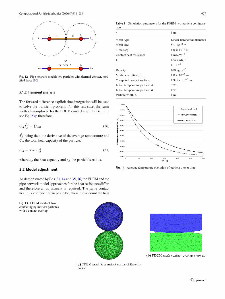
5.1 The pipe networkmodel (Y. T. Feng 2009 [10])

5.1.1 Model description

The pipe network model presented by Y.T. Feng [9,10] isdesigned for the modelling of large numbers of circular par-ticles in 2D as it would represent long or infinite pipes. Thismethod is presented in the culture of the discrete elementmethod and is introduced here to form the basis of a valida-tion study of the new FDEM method. Consider two circular

Fig. 11 Contact heat flux for the discrete thermal element, modifiedfrom [9]

particles A and B having respectively TA and TB as averagetemperatures; the thermal resistances of the two pipes are,respectively, RA and RB . The total thermal resistance is:

RAB = RA + RB + R∗c (33)

where R∗c the contact thermal resistance for the pipe network

model. The contact zone of the discrete thermal element isrepresented by an arc on the boundary of the element whichis defined with its half angle αi , see Fig. 11. For angles ofcontact below 30◦, the discrete element thermal resistancecan be approximated with high accuracy by the formula:

RA = 1

πkA

(−lnαA + 3

2+ α2

A

36

)(34)

where kA, the thermal conductivity of particle A.The boundaries of the particles are insulated and heat

transfers only through the contact zone. For two contactingdiscrete thermal element (see Fig. 12), the heat flow betweenthe two particles QAB is defined as follows :

(TB − TA) = RAB QAB (35)

Table 2 Average error of FEMand FDEM simulations in theanalytical solution

Times Average absolute error

Mesh size: 1.10−1 m Mesh size: 5.10−2 m

FEM FDEM FEM FDEM

10 s 0.642 % 0.489 % 0.077 % 0.167 %

50 s 0.009 % 0.098 % 0.005 % 0.050 %

100 s 0.005 % 0.035 % 0.003 % 0.018 %

Computationalrun times (min)Intel Xeon (R)CPU E5-26302.30 GHz proces-sor

2.30 5.10 21.40 31.50

123


Fig. 12 Pipe network model: two particles with thermal contact, mod-ified from [10]

5.1.2 Transient analysis

The forward difference explicit time integration will be usedto solve the transient problem. For this test case, the samemethod is employed for the FDEMcontact algorithm (θ = 0,see Eq. 23); therefore,

CAT 0A = QAB (36)

TA being the time derivative of the average temperature andCA the total heat capacity of the particle:

CA = πρcpr2A (37)

where cp the heat capacity and rA the particle’s radius.

5.2 Model adjustment

Asdemonstrated byEqs. 21, 14 and 35, 36, the FDEMand thepipe network model approaches for the heat resistance differ,and therefore an adjustment is required. The same contactheat flux contribution needs to be taken into account the heat

Table 3 Simulation parameters for the FDEM two-particle configura-tion

r 1 m

Mesh type Linear tetrahedral elements

Mesh size 8 × 10−2 m

Time step 1.0 × 10−3 s

Contact heat resistance 1 mK.W−1

k 1 W.(mK)−1

c 1 J.K−1

Density 100 kg.m−3

Mesh penetration, p 1.0 ∗ 10−2 m

Computed contact surface 1.925 ∗ 10−2 m

Initial temperature particle A 0◦CInitial temperature particle B 1◦CParticle width L 1 m

Fig. 14 Average temperature evolution of particle j over time

Fig. 13 FDEM mesh of twocontacting cylindrical particleswith a contact overlap

123


Fig. 15 Initial, transient andfinal state of the pipe networkvalidation simulation

diffusion equation; therefore, the following condition has tobe fulfilled:

QAB = 1

wcylBc (38)

The left-hand side of the above equation is the heat flux con-tribution from the pipe network model extended from a 2Ddisc to an hypothetical 3D cylinder of a width represented bywcyl ; the right-hand side corresponds to the FDEM model.Therefore, we write:

T 0B − T 0

A

RAB= 1

wcyl

ΔTc ScRc

(39)

We can also write:

RAB = Rc wcyl

Sc− RA − RB (40)

This conclusion also implies that TB −TA = ΔTc, i.e. theparticle average temperature difference is equal to the localtemperature difference at the contact zone and such is themain approximation of the discrete element approach; thiscondition will only be verified when the thermal conductivi-ties are high compared to the contact heat resistance. Tomakesure this assumption is acceptable in the following simula-tion, in addition to theΔTc local temperature gap calculation,a ΔTc calculation based on the particle average temperaturedifference has also been implemented in FDEM, the code tocompare with the pipe network model.

5.3 FDEM contact simulation settings

In order to make possible a comparison between the simula-tion of the 2D problem of two contacting discs and the new3D contact heat transfer FDEM, we define two contactingthin cylinders of the same radius r and width wcyl . The two

finite elementmeshes are overlapping at the contact zone, seeFig. 13. Simulation parameters are summarised in Table 3.Two different FDEM simulations were performed, the firstwith a contact heat flux calculated with the local tempera-tures, the second calculated with the average temperatures.

The accuracy of the computed contact surface Sc is vali-dated against a theoretical surface formula Sthc obtained fromthe overlap of two circles:

sin αthA = 1

2 d rA

(4 d2 r2A − (d2 − r2A + r2B)2

)(41)

Sthc = 2 αthA rA L (42)

where d = rA + rB − p, p being the penetration of the twomeshes. For the actual configuration, the theoretical surface isSthc = 0.02m2, and the error of the computed contact surfaceis therefore of 4%. Again that error is only due to the finiteelement approximation of the domain. Contact surface errorreduces to 0.4%with a two-time smaller mesh. Nevertheless,to reduce errors for this validation test, the computed contactsurface is transformed into the equivalent contact half angleand then imputed in the pipe network model by means of theformula:

αA = Sc2 wcyl rA

(43)

The two particles with different temperature are in contactinitially. Figure 14 shows the evolution of the temperaturechanges against time. Results of the temperature are pre-sented for particle B in Fig. 14. We obtain an average errorof 7.6 % between the pipe network model and the origi-nal FDEM (with a local temperature difference) against anaverage error of 0.63%with FDEMwith the particle averagetemperature difference. In this configuration, it is evident thatthe main assumption of the pipe network model, being theconsideration of the particle’s temperature to be uniform, isnot valid as the heat conductivity is relatively small (Fig. 15).

123


Fig. 16 Average temperature evolution of particle j over time with anincreased heat conductivity

Fig. 17 Particle mesh (metal nut shape) composed of 192 tetrahedralfinite elements

We consider now the same configuration with a heat con-ductivity a hundred times greater, and results are presentedin Fig. 16. In this case, both FDEM simulations producethe same result with an average error of 0.7 %; hence, thepipe network approximation can here be considered valid.In summary, the foregoing examples show that when signif-icantly varying temperatures exist in the contacting bodies,the FDEM code can capture the complexity of the time his-tory, giving quite different results when the assumption ofaverage temperature within the particle is imposed.

Table 4 Simulation parameters of the multibody simulation

Nut inner radius 0.026 m

Nut outer width 0.04 m

Container inner diameter 0.45 m

Container wall thickness 0.02m

Contact heat resistance 0.01 mKW−1

Heat conductivity k 0.001 W.(mK)−1

Heat capacity c 1 J.K−1

Density 1000 kg.m−3

Young’s modulus 7.5 GPa

Poisson’s ratio 0.22

Penalty force 0.75 MPa

Time step size 1s

Number of time steps 80

6 Multibody simulation

This section presents a static multibody heat transfer simula-tionwith 2000 particles packed up into a cylindrical containerwhich is heated from the outside. To obtain such a configura-tion, the particles are dropped into the container usingFDEM.After all the particles are deposited, a fixed temperatureboundary condition of 300◦C is applied to the container. Notethat for this simulation, only heat conduction heat transferis considered. Moreover, the system is static during heatingbecause thermal expansion effects are not taken into account.The deposited particles are in the shape of a metal nut, andtheir mesh is composed of 192 elements (see Fig. 17). Simu-lation properties are listed in Table 4. Finally, Figs. 18 and 19show the heat transfer simulation with the nut particles beingheated up from 0 to 300◦C (Fig. 20).

7 Conclusion

Anew3Dapproach is presented in this paper, first with a one-dimensional heat conduction validation test that has provento give very accurate results. However, we are aware that thissimulation was for a perfect contact; thus, a very low con-tact resistivity was chosen. For this reason, the temperatureson both sides of the contact zone are almost the same andwe have a temperature continuity; thus, FEM and FDEMproduce a very similar result. This first validation case isstrengthened with a second successful one which is a real-istic contact problem as a higher thermal resistivity is set.The FDEM approach has offered here more flexibility thana discrete element approach as it can consider cases wherethe average temperature is not representative of the problem.Thismeans FDEMcanmodel problemswith extreme bound-ary conditions and complex particle heat distributions with

123


Fig. 18 Thermal simulationset-up of 2000 nut particlesinside a cylindrical container

123


Fig. 19 Heating up simulationof 2000 nut particles asperformed on a Intel Xeon (R)CPU E5-2630 2.30GHzprocessor (cross section view)

123


Fig. 20 Heating up simulationof 2000 nut particles asperformed on a Intel Xeon (R)CPU E5-2630 2.30 GHzprocessor

123


accuracy. Finally, as the multibody simulation demonstrates,FDEM can handle large sets of particles and compute thethermal distribution at desired times. The strength of FDEMis also that it can be coupled with existing fracture, plasticityand thermal expansion models. Hence, it is critical for thefuture of this method to provide a more detailed understand-ing of the linkage between contact force and heat resistancewhich has been so far been neglected in thiswork and requiresfurther theory and method for implementation.

8 Future work

As the FDEM method presented here is already capableof tackling multibody dynamic problems, future work willinclude such simulations with heat transfer. We have pre-sented here the process to capture the contact area of twopenetrating meshes; however, it is dependent on the penaltyfunction method [21] and the amount of mesh penetration.Hence, it is important to investigate the sensitivity of thesurface calculation to the mesh penetration. The role of thepenalty function is to calculate element-to-element intersec-tion for the contact force. Therefore, it will be powerful toinsert in this method an empirical law linking the element-to-element intersection to the heat resistance and contact surfacesuch as in Bahrami et al. works [3]. Finally, the contact heattransfer method will be validated further in more complexconfigurations and with experimental results. To validate thecontact heat transfer, suitable experiments can be selectedfrom those performed in a vacuum [6] or where conductionheat transfer is largely dominant [32].

Acknowledgements We acknowledge the Natural EnvironmentResearch Council, Radioactive Waste Management Limited and Envi-ronment Agency for the funding received for the HydroFrame project,NE/L000660/1, through theRadioactivity and the Environment (RATE)programme.

Compliance with ethical standards

Conflict of interest The authors declare that they have no conflict ofinterest.

Open Access This article is licensed under a Creative CommonsAttribution 4.0 International License, which permits use, sharing, adap-tation, distribution and reproduction in any medium or format, aslong as you give appropriate credit to the original author(s) and thesource, provide a link to the Creative Commons licence, and indi-cate if changes were made. The images or other third party materialin this article are included in the article’s Creative Commons licence,unless indicated otherwise in a credit line to the material. If materialis not included in the article’s Creative Commons licence and yourintended use is not permitted by statutory regulation or exceeds thepermitted use, youwill need to obtain permission directly from the copy-

right holder. To view a copy of this licence, visit http://creativecommons.org/licenses/by/4.0/.

References

1. Williams J, Pentland A (1992) Superquadrics and modal dynamicsfor discrete elements in interactive design. Eng Comput 9(2):115–127

2. Argento C, Bouvard D (1996) Modeling the effective thermal con-ductivity of random packing of spheres through densification. IntJ Heat Mass Transf 39(7):1343–1350

3. Bahrami M, Culham JR, Yovanovich MM (2004) Modeling ther-mal contact resistance: a scale analysis approach. J Heat Transfer126(6):896–905

4. Bathe KJ, Bouzinov Pa, Pantuso D (2000) A finite element pro-cedure for the analysis of thermo-mechanical solids in contact.Comput Struct 75:551–573

5. Bergman TL, Incropera FP, Lavine AS (2011) Fundamentals ofheat and mass transfer. Wiley, Hoboken

6. Chan CK, Tien CL (1973) Conductance of packed spheres invacuum. J Heat transf 95(3):302–308. https://doi.org/10.1115/1.3450056

7. Cheng GJ, Yu AB, Zulli P (1999) Evaluation of effective thermalconductivity from the structure of a packed bed. Chem Eng Sci54:4199–4209

8. Favier JF,Abbaspour-FardMH,KremmerM(2001)Modeling non-spherical particles usingmultisphere discrete elements. J EngMech127(10):971–977

9. Feng YT, Han K, Li CF, Owen DRJ (2008) Discrete thermalelement modelling of heat conduction in particle systems: Basicformulations. J Comput Phys 227(10):5072–5089

10. FengYT,HanK,OwenDRJ (2009)Discrete thermal elementmod-elling of heat conduction in particle systems: pipe-network modeland transient analysis. Powder Technol 193(3):248–256

11. Gan J, Zhou Z, Yu A (2016) Particle scale study of heat transfer inpacked and fluidized beds of ellipsoidal particles. Chem Eng Sci144:201–215

12. Govender N,Wilke DN,Wu CY, Khinast J, Pizette P, XuW (2018)Hopper flow of irregularly shaped particles (non-convex polyhe-dra): gpu-based dem simulation and experimental validation. ChemEng Sci 188:34–51

13. Govender N, Wilke DN, Wu CY, Tuzun U, Kureck H (2019) Anumerical investigation into the effect of angular particle shape onblast furnace burden topography and percolation using a gpu solveddiscrete element model. Chem Eng Sci 204:9–26

14. Hyun S, Pel L, Molinari JF, Robbins MO (2004) Finite-elementanalysis of contact between elastic self-affine surfaces. Phys RevE 70(22):1–12

15. Jagota A,Mikeska K, Bordia R (1990) Isotropic constitutivemodelfor sintering particle packings. J Am Ceram Soc 73(8):2266–2273

16. JiaX,GopinathanN,WilliamsRA (2002)Modeling complex pack-ing structures and their thermal properties. Adv Powder Technol13(1):55–71

17. Johansson L, Klarbring A (1993) Thermoelastic frictional contactproblems: modelling, finite element approximation and numericalrealization. Comput Methods Appl Mech Eng 105(2):181–210

18. Lewis RW, Morgan K, Thomas H, Seetharamu K (1996) The finiteelement method in heat transfer analysis. Wiley, Hoboken

19. Mikic B, Rohsenow W (1966) Thermal contact resistance. Tech-nical Report DSR 74542–41(September)

20. Munjiza A (2004) The combined finite–discrete element method.Wiley, Hoboken

123

http://creativecommons.org/licenses/by/4.0/

http://creativecommons.org/licenses/by/4.0/

https://doi.org/10.1115/1.3450056

https://doi.org/10.1115/1.3450056


21. Munjiza A, Andrews K (2000) Penalty function method for com-bined finite-discrete element systems comprising large number ofseparate bodies. J Numer Methods Eng 49(11):1377–1396

22. Murashov MV, Panin SD (2015) Numerical modelling of contactheat transfer problem with work hardened rough surfaces. Int JHeat Mass Transf 90:72–80

23. Nikishkov G (2010) Finite element equations for heat transfer. In:Programming finite elements in javaTM. Springer, London, pp. 13–19. https://doi.org/10.1007/978-1-84882-972-5_2

24. Oysu C (2007) Finite element and boundary element contactstress analysis with remeshing technique. Appl Math Model31(12):2744–2753

25. Rickelt S,Kruggel-EmdenH,Wirtz S, SchererV (2009) Simulationof heat transfer in moving granular material by the discrete elementmethod with special emphasis on inner particle heat transfer. In:Proceedings of the ASME 2009 heat transfer summer conferencepp. 1–11

26. Rickelt S, Wirtz S, Scherer V (2008) A new approach to simu-late transient heat transfer within the discrete element method. In:PressureVessels andPipingConference,Volume4: Fluid-StructureInteraction. pp. 221–230. https://doi.org/10.1115/PVP2008-61522

27. Sahoo P, Ghosh N (2007) Finite element contact analysis of fractalsurfaces. J Phys D Appl Phys 40(14):4245–4252

28. SchererV,Wirtz S,KrauseB,WissingF (2017) Simulation of react-ing moving granular material in furnaces and boilers an overviewon the capabilities of the discrete elementmethod. Energy Procedia120:41–61 INFUB - 11th European Conference on IndustrialFurnaces and Boilers, INFUB-11

29. Seelen L, Padding J, Kuipers J (2018) A granular discrete elementmethod for arbitrary convex particle shapes: method and packinggeneration. Chem Eng Sci 189:84–101

30. Siu WWM, Lee SHK (2004) Transient temperature computationof spheres in three-dimensional random packings. Int J Heat MassTransf 47(5):887–898

31. Yastrebov VA, Durand J, Proudhon H, Cailletaud G (2011) Roughsurface contact analysis by means of the finite element methodand of a new reduced model. Comptes Rendus Mécanique 339(7–8):473–490

32. Zhang R, Yang H, Lu J,WuY (2013) Theoretical and experimentalanalysis of bed-to-wall heat transfer in heat recovery processing.Powder Technol 249:186–195

Publisher’s Note Springer Nature remains neutral with regard to juris-dictional claims in published maps and institutional affiliations.

123

https://doi.org/10.1007/978-1-84882-972-5_2

https://doi.org/10.1115/PVP2008-61522

capturing heat transfer for complex-shaped multibody

Documents