capturing structural distortions in digital images and videos
TRANSCRIPT

CAPTURING STRUCTURAL DISTORTIONS IN
DIGITAL IMAGES AND VIDEOS
by
Peng Peng
B.Eng., University of Science and Technology of China, 2010
a Thesis submitted in partial fulfillment
of the requirements for the degree of
Master of Science
in the
School of Computing Science
Faculty of Applied Sciences
c© Peng Peng 2012
SIMON FRASER UNIVERSITY
Fall 2012
All rights reserved.
However, in accordance with the Copyright Act of Canada, this work may be
reproduced without authorization under the conditions for “Fair Dealing.”
Therefore, limited reproduction of this work for the purposes of private study,
research, criticism, review and news reporting is likely to be in accordance
with the law, particularly if cited appropriately.
APPROVAL
Name: Peng Peng
Degree: Master of Science
Title of Thesis: Capturing Structural Distortions in Digital Images and Videos
Examining Committee: Dr. Richard Vaughan, Associate Professor, Computing Sci-
ence
Simon Fraser University
Chair
Dr. Ze-Nian Li, Professor, Computing Science
Simon Fraser University
Senior Supervisor
Dr. Greg Mori, Associate Professor, Computing Sci-
ence
Simon Fraser University
Supervisor
Dr. Mark Drew, Professor, Computing Science
Simon Fraser University
SFU Examiner
Date Approved:
ii

Partial Copyright Licence
iii

Abstract
With the growing demand for image and video services, objective analysis of image and
video quality has received increased interest from the content providers and network op-
erators. This study proposes to capture structural image/video distortions through spa-
tial/spatiotemporal orientation analysis. For image quality assessment (IQA), we signif-
icantly improve the classic SSIM algorithm with low computational overhead by taking
into account the preservation of edge orientations. For video quality assessment (VQA),
a unified framework for attention guided structural distortion measure is presented based
on the motion-tuned spatiotemporal oriented energies and a spatiotemporal visual saliency
model, in which the descriptive and efficient distributed motion representation is employed
to alleviate the typical problems of the commonly used optical flow methods. The struc-
tural distortion measure is then combined with a multi-scale SSIM based spatial distortion
measure to form a comprehensive video distortion metric, which demonstrates good quality
prediction and high computational efficiency.
Keywords: Image quality assessment; video quality assessment; edge orientation anal-
ysis; spatiotemporal oriented energies; visual saliency
iv

To my parents and sister!
v

Acknowledgments
My greatest thank goes to my advisor and mentor, Dr. Ze-Nian Li, who has always been very
supportive and patient during my graduate study at SFU. I appreciate the great amount of
precious time that he has spent on my research through our regular and random meetings
and emails. I benefit greatly from his professional and inspirational guidance. Without his
valuable help in all kinds of ways, this thesis would never have been possible. Meanwhile, I
would like to thank my supervisor, Dr. Greg Mori, and examiner, Dr. Mark Drew, for their
insightful comments and encouraging words. I am also grateful to Dr. Richard Vaughan for
his precious time on chairing my examining committee.
I like to thank Dr. Kevin Cannons for the helful discussions and suggestions on this
work. I very much appreciate his knowledgeable and patient repsonses to my questions.
Thanks to Jianqiao Li for her great help on improving the quality of this thesis and the
slides for the defence. Thanks to Peng Wang for his time on the proof-reading of the first
and third chapters of this thesis, and to Guangtong Zhou for the helpful comments on the
slides. I also like to thank Dr. Konstantinos Derpanis from York University for providing
me with the code of the motion model and some of the visualizations in Chapter 3. Thanks
to Prof. Zhou Wang at the University of Waterloo for giving me the permission to use in
this thesis some of the figures from his work on image quality assessment.
I would also like to take this opportunity to thank all the colleagues in the Vision and
Media Lab (VML) in SFU. Thanks to them for being so nice and making VML such a
delightful place to work at. Special thanks to Dr. Kevin Cannons, Arash Vahdat, Yasaman
Sefidgar, Nataliya Shapovalova, Guangtong Zhou, and Jianqiao Li for all the helpful sugges-
tions and comments during my rehearsal defence. Thanks to all my friends for their support
through the difficult times, and for all the joyful things we did together.
Finally, my deepest gratitude goes to my family, for their love, support, and sacrifices.
vi

Contents
Approval ii
Partial Copyright License iii
Abstract iv
Dedication v
Acknowledgments vi
Contents vii
List of Tables ix
List of Figures x
1 Introduction 1
1.1 HVS-oriented approach and engineering approach . . . . . . . . . . . . . . . . 2
1.2 Structural information in images and videos . . . . . . . . . . . . . . . . . . . 4
1.3 Contributions . . . . . . . . . . . . . . . . . . . . . . . . . . . . . . . . . . . . 7
1.4 Organization . . . . . . . . . . . . . . . . . . . . . . . . . . . . . . . . . . . . 7
2 Image quality assessment 8
2.1 Motivation . . . . . . . . . . . . . . . . . . . . . . . . . . . . . . . . . . . . . 8
2.2 Related work . . . . . . . . . . . . . . . . . . . . . . . . . . . . . . . . . . . . 9
2.3 Proposed method . . . . . . . . . . . . . . . . . . . . . . . . . . . . . . . . . . 11
2.3.1 Capturing structural distortions along edges . . . . . . . . . . . . . . . 11
vii

2.3.2 Amendment of the SSIM indexes . . . . . . . . . . . . . . . . . . . . . 12
2.4 Evaluation . . . . . . . . . . . . . . . . . . . . . . . . . . . . . . . . . . . . . . 14
2.4.1 Datasets . . . . . . . . . . . . . . . . . . . . . . . . . . . . . . . . . . . 14
2.4.2 Quality prediction performance . . . . . . . . . . . . . . . . . . . . . . 15
2.4.3 Computational efficiency . . . . . . . . . . . . . . . . . . . . . . . . . . 18
2.5 Summary . . . . . . . . . . . . . . . . . . . . . . . . . . . . . . . . . . . . . . 19
3 Video quality assessment 21
3.1 Motivation . . . . . . . . . . . . . . . . . . . . . . . . . . . . . . . . . . . . . 21
3.2 Related work . . . . . . . . . . . . . . . . . . . . . . . . . . . . . . . . . . . . 24
3.2.1 Motion modeling based VQA methods . . . . . . . . . . . . . . . . . . 24
3.2.2 Visual attention based VQA methods . . . . . . . . . . . . . . . . . . 26
3.3 Capturing motion-related structural distortions . . . . . . . . . . . . . . . . . 27
3.3.1 Motion-tuned spatiotemporal oriented energies . . . . . . . . . . . . . 27
3.3.2 Self-information based bottom-up spatiotemporal saliency . . . . . . . 31
3.3.3 Attention-guided spatial pooling . . . . . . . . . . . . . . . . . . . . . 33
3.4 Overall video quality prediction . . . . . . . . . . . . . . . . . . . . . . . . . . 34
3.4.1 Temporal variations of video quality . . . . . . . . . . . . . . . . . . . 34
3.4.2 Incorporating spatial quality . . . . . . . . . . . . . . . . . . . . . . . 35
3.5 Evaluation . . . . . . . . . . . . . . . . . . . . . . . . . . . . . . . . . . . . . . 36
3.5.1 Datasets . . . . . . . . . . . . . . . . . . . . . . . . . . . . . . . . . . . 36
3.5.2 Quality prediction performance . . . . . . . . . . . . . . . . . . . . . . 37
3.5.3 Computational efficiency . . . . . . . . . . . . . . . . . . . . . . . . . . 39
3.6 Summary . . . . . . . . . . . . . . . . . . . . . . . . . . . . . . . . . . . . . . 40
4 Conclusions and future work 43
Bibliography 45
viii

List of Tables
2.1 Description of the image quality databases (Nri: Number of reference images;
Ndi: Number of distorted images; Ndt: Number of distortion types) . . . . . . 15
2.2 Performance on LIVE . . . . . . . . . . . . . . . . . . . . . . . . . . . . . . . 17
2.3 Performance on CSIQ . . . . . . . . . . . . . . . . . . . . . . . . . . . . . . . 17
2.4 Performance on TID-7 . . . . . . . . . . . . . . . . . . . . . . . . . . . . . . . 18
2.5 Performance on TID . . . . . . . . . . . . . . . . . . . . . . . . . . . . . . . . 18
3.1 Performance of the proposed methods on the LIVE video quality database . . 38
ix

List of Figures
1.1 Framework of objective visual quality assessment. . . . . . . . . . . . . . . . . 3
1.2 Structural distortions characterized by the SSIM index. In the absolute differ-
ence map and the SSIM index map, low intensity values indicate poor quality.
(Reprinted, with permission, from “Spatial pooling strategies for perceptual
image quality assessment” by Wang and Shang, ICIP, 2006 [84].) . . . . . . 5
1.3 Comparison of “Boat” images with different types of distortions, all with
MSE = 200. (a) Original image; (b) Contrast change, SSIM = 0.9168; (c)
Mean-shifted, SSIM = 0.9900; (d) JPEG Compression, SSIM = 0.6949; (e)
Blurred: SSIM = 0.7052; (f) Salt-pepper impulsive noise: 0.7748. (Reprinted,
with permission, from “Image quality assessment: from error visibility to
structural similarity” by Wang et al., IEEE Transaction on Image Processing,
2004 [80].) . . . . . . . . . . . . . . . . . . . . . . . . . . . . . . . . . . . . . 6
2.1 Comparison between the MS-SSIM index and the proposed R-MSSSIM method. 13
2.2 Some exotic distortions from the TID database. . . . . . . . . . . . . . . . . . 19
2.3 Running time for the image quality metrics. . . . . . . . . . . . . . . . . . . . 20
3.1 Flowchart of the proposed video quality metric. . . . . . . . . . . . . . . . . . 23
3.2 An illustration of the appearance marginalization in the frequency domain.
Left: A set of N + 1 equally spaced N -th derivative of Gaussian filters con-
sistent with a certain frequence plane; Right: The sum of the N+1 energy
samples corresponds to computing the energy along the surface of a smooth
ring-shaped function. (Reprinted, with permission, from “On the Role of
Representation in the Analysis of Visual Spacetime” by Konstantinos Derpa-
nis, PhD Thesis, 2010 [22].) . . . . . . . . . . . . . . . . . . . . . . . . . . . 29
x

3.3 Man jumping into water with a big splash, captured by a stationary cam-
era. Top-Left (original frame), top-right (SICOM ), bottom-left (SIMC), and
bottom-right (SIM ). . . . . . . . . . . . . . . . . . . . . . . . . . . . . . . . 32
3.4 Moving camera tracking a plane. Top-Left (original frame), top-right (SICOM ),
bottom-left (SIMC), and bottom-right (SIM ). . . . . . . . . . . . . . . . . . . 33
3.5 Wavy water with high contrast area, captured by a stationary camera. Top-
Left (original frame), top-right (SICOM ), bottom-left (SIMC), and bottom-
right (SIM ). . . . . . . . . . . . . . . . . . . . . . . . . . . . . . . . . . . . . . 34
3.6 SRCC (top) and PLCC (bottom) on the entire LVIE video quality database. 42
xi

Chapter 1
Introduction
With the explosion of multimedia applications in recent years due to the advances of wired
and wireless communication networks, digital images and videos have become increasingly
popular in people’s daily life. Before the multimedia contents reach the end users, they typ-
ically pass through several processing stages that result in impairment of quality (e.g., lossy
source encoding and transmission over error prone channels). Methods for evaluating image
and video quality have received growing interest from content providers and network oper-
ators, as they play a crucial role in Quality-of-Service (QoS) monitoring, and performance
evaluation and perceptually optimal design of systems for image/video processing. A group
of experts known as the Video Quality Experts Group (VQEG) [1] have made lots of efforts
in the search for image and video quality measures suitable for standardization. However,
due to the difficulty in measuring the quality of visual signals, the standardisation process
for image and video is somewhat slower, when it is compared with the already standardized
perceptual metrics for audio and speech [79, 28, 69].
Intuitively, the best judgment of image and video quality is the human opinion on
the perceived quality, which is also known as the ”subjective quality”. Subjective quality
assessment typically involves experiments that require a group of human observers to vote
for the quality of a medium. The votes are then pooled into a mean opinion score (MOS) to
provide a measure of the subjective quality of the test medium [3, 69]. Though subjective
methods have been used for many years as the most reliable form of visual assessment, it
requires human viewers working in a long period on repeated experiments, which makes it
time-consuming and expensive, hence impracticable for many scenarios, such as real-time
systems. In contrast, objective methods are automated algorithms that attempt to predict
1

CHAPTER 1. INTRODUCTION 2
image or video quality in a way consistent with the human perception. As a result, the
effectiveness of an objective quality metric is evaluated by how well the predicted quality
correlates with the human-supplied subjective quality. Clearly, an effective objective method
can have a much more extended field of applications than the subjective methods.
Depending on the presence of a reference signal (i.e. image or video), the objective qual-
ity assessment methods can be divided into three classes: full-reference, reduced-reference,
and no-reference. An illustration of this categorization is shown in Fig. 1.1. For the first
type, a “perfect-quality” reference signal is available for comparison during the assessment
of a test signal. The goal of full-reference methods is to evaluate the fidelity of the distorted
signal with respect to the reference signal. Reduce-reference methods operates with partial
information about the reference signal, which are usually quality features extracted from
a reference image or video. No-reference methods, also known as blind methods, attempt
to evaluate image/video quality without any information other than the test signal, which
is considered to be a much more challenging task, especially for video quality assessment.
Before generic blind methods become feasible, there is much yet to be studied regarding
full-reference and reduced-reference quality assessment [9]. In this study, we focus on the
full-reference objective algorithms for image and video quality assessment.
1.1 HVS-oriented approach and engineering approach
Generally speaking, there are two approaches for objective visual quality assessment, includ-
ing the human vision system (HVS)-oriented approach and engineering approach [9, 28, 31].
The HVS-oriented approach attempts to model the various stages of processing that oc-
cur in the HVS, such as multi-channel decomposition, contrast sensitivity, spatial/temporal
masking effects, and so on [9, 31]. Typically, the reference and test signals are passed
through a computational model of the visual pathway. The visual quality is defined as an
error measure between the two signals at the output of the model. Popular HVS-oriented
methods include the Moving Pictures Quality Metric (MPQM) [76], Perceptual Distortion
Metric (PDM) [90], and the Digital Video Quality Metric (DVQ) [89]. For instance, the
MPQM method [76] is one of the first HVS-oriented methods for video quality assessment.
It first conducts a multi-channel decomposition of the video signals using a Gabor filter-
bank in the spatial domain and two filters (one bandpass and one lowpass) in the temporal
domain. Then the contrast sensitivity and masking effects are considered in each of the

CHAPTER 1. INTRODUCTION 3
Figure 1.1: Framework of objective visual quality assessment.
channels resulting in weights for error normalization. Finally, a local distortion measure is
obtained by pooling the errors over the channels.
While much work in the literature has been focused on modeling the HVS for designing
objective IQA and VQA metrics, there has been a shift towards techniques that attempt
to characterize features which the human eye associates with loss of quality [9]. These
techniques are referred to as engineering methods, also known as feature-based methods.
Part of the reason for this shift lays in the complexity and incompleteness of the HVS
models. A more important reason is that typical HVS-oriented methods suffer from the
“supra-threshold” problem [80, 68]. Specifically, given that the HVS-oriented methods are
primarily designed to model threshold psychophysics, i.e., estimating the threshold at which
a stimulus is just barely visible, they exhibit limited effectiveness when the distortions are

CHAPTER 1. INTRODUCTION 4
significantly larger than the threshold levels. One typical engineering method is the well
recognized Structural SIMilarity (SSIM) index [80, 83], which performs separate comparisons
of luminance, contrast and structure between a reference image and a test image. The Video
Quality Metric (VQM) [60] is another popular engineering method that has been adopted as
a North American standard by the American National Standards Institute (ANSI) in 2003.
It extracts seven features from the reference and/or test videos, including four features
extracted from the spatial gradients of the luminance component, two features extracted
from the chrominance component, and one feature that captures contrast and temporal
information.
While HVS-oriented methods are often complex and computational expensive, engineer-
ing methods span from very simple numeric measures to highly complex algorithms. It is
worth mentioning that there is no clear boundary between the HVS-oriented approach and
engineering approach. Certain characteristics of the HVS can be considered in the design of
engineering methods as well. In other words, methods following either approach can benefit
from a better understanding of the HVS.
1.2 Structural information in images and videos
The environment surrounding us is neither arbitrary nor random, rather it is highly struc-
tured by the physical, biological, and many other forces in the world [74, 22]. As a result,
natural image/video signals are highly structured in that their pixels exhibit strong depen-
dencies, especially when they are spatially close. It is this structure that facilitates reliable
inferences of our environment from raw image signals [91, 65, 4]. Based on the hypothe-
sis that the human vision system is highly adapted for extracting structural information,
Wang et al. propose the SSIM index [80] for IQA, in which they define the structural in-
formation in an image as those attributes that represent the structure of objects in a scene,
independent of the average luminance and contrast. An illustration of its efficacy in cap-
turing the structural distortions is given in Fig. 1.2. It is easy to see that the SSIM index
does a better job than the absolute difference map in capturing the structural distortions,
such as the blockiness in the sky. With its prominent quality-prediction ability, the SSIM
index represents a significant step forward from the traditional mean square error (MSE)
based engineering IQA metrics, such as the peak signal-to-noise ratio (PSNR). A convincing
illustration is given in Fig. 1.3.

CHAPTER 1. INTRODUCTION 5
Figure 1.2: Structural distortions characterized by the SSIM index. In the absolute differ-ence map and the SSIM index map, low intensity values indicate poor quality. (Reprinted,with permission, from “Spatial pooling strategies for perceptual image quality assessment”by Wang and Shang, ICIP, 2006 [84].)
In this thesis, we have adopted the word ”structural” from the SSIM (Structural SIM-
ilarity) index, as our methods also attempt to capture the attributes of visual scenes that
are invariant to the additive luminance change and contrast change. Unlike the SSIM index
that relies on a simple block-based analysis of image statistics, our methods characterize
the structural information in visual scenes based on a spatial/spatiotemporal orientation
analysis, because the orientation features are more closely related to the image and video
structure, such as the object shape, texture, and motion direction. Moreover, it is known
that a variety of neurons in the HVS are orientation selective. Hubel and Wiesel show that
one of the major transforms accomplished by the visual cortex is the rearrangement of in-
coming information so that most of its cells respond not to a spot of light but to specifically
oriented line segments [34]. Later work shows that simple cells in the visual cortex act more
or less like linear filters, which can be well modeled by Gabor filters [21]. In addition, a
large population of neurons that are devoted to motion perception are known to be direc-
tionally selective. To analyze visual motion, the visual system first filters the input signal
in both space and time to compute the motion of oriented elements in visual scenes. This
computation is represented by the activity of neurons in the primary visual cortex (V1).
As the components of a moving pattern can move in different directions, the motion signals
from multiple V1 cells are then combined to compute the pattern motion, which is done by

CHAPTER 1. INTRODUCTION 6
Figure 1.3: Comparison of “Boat” images with different types of distortions, all with MSE= 200. (a) Original image; (b) Contrast change, SSIM = 0.9168; (c) Mean-shifted, SSIM =0.9900; (d) JPEG Compression, SSIM = 0.6949; (e) Blurred: SSIM = 0.7052; (f) Salt-pepperimpulsive noise: 0.7748. (Reprinted, with permission, from “Image quality assessment:from error visibility to structural similarity” by Wang et al., IEEE Transaction on ImageProcessing, 2004 [80].)
a variety of the directionally selective neurons in the extrastriate area MT (V5) [66].
In the context of IQA, we capture structural distortions based on the edge orientations, as
it is believed that the HVS heavily relies on edges and contours to perceive the structure of a
scene [26, 51]. In the context of VQA, we measure the spatiotemporal oriented energies along
the motion trajectories with a bias towards the areas of attention, aiming to capture the
motion-related structural distortions in videos and to heavily penalize structural distortions
that occur in the areas of attention.

CHAPTER 1. INTRODUCTION 7
1.3 Contributions
In this thesis, we approach full-reference objective assessment of image and video quality
from a primarily engineering standpoint, as well as by taking into account some character-
istics of the HVS. Our work focuses on capturing the structural distortions in images and
videos through spatial/spatiotemporal orientation analysis. The contributions of this thesis
mainly include three parts:
• Firstly, we propose an effective approach to enhance the performance of the classic
SSIM indexes by taking into account the preservation of edge orientations with im-
pressively low computational overhead.
• Secondly, we propose an effective and efficient VQA method, in which a unified frame-
work based on spatiotemporal analysis is developed for attention guided and motion
tuned measure of motion-related structural distortions.
• Last but not the least, we employ a reliable distributed representation [24, 22, 25]
for motion modeling, which alleviates the typical problems of the optical-flow based
methods that are commonly used in the context of VQA.
1.4 Organization
Chapter 1 gives an introduction to image and video quality assessment. Chapter 2 presents a
very simple full-reference objective IQA metric [59], which amends the SSIM indexes [80, 85].
Chapter 3 first introduces a motion-tuned local quality measure to capture the motion-
related structural distortions (i.e. temporal distortions) in videos. Then spatiotemporal
saliency models are built based on the self-information of the motion descriptors, which is
used to pool the local quality measures into frame-level quality scores. Finally, a compre-
hensive video quality metric is developed by taking into account the spatial quality and
temporal variations of quality. Chapter 4 summarizes the thesis and provides suggestions
for future investigation. The motivations and related work are presented in each individual
chapter.

Chapter 2
Image quality assessment
2.1 Motivation
A good image quality metric should correlate well with the human perception of image qual-
ity. Based on the assumption that the human vision system (HVS) is highly adapted for
extracting structural information from a scene, Wang et al. propose the structural similarity
(SSIM) indexes [80, 85] that are widely recognized for their remarkably better correlation
with the human perception of image quality than the traditional mean square error (MSE)
based metrics. However, with the development of modern image quality metrics, some newer
methods stand out with better quality-prediction accuracy [46, 72, 40]. The Visual Infor-
mation Fidelity (VIF) method [72] proposed by Sheikh and Bovik evaluates image quality
by measuring the amount of information about the reference image that can be extracted
from the test image based on a sophisticated vector Gaussian Scale Mixture (GSM) model.
It is reported that their method achieves significantly better quality-prediction performance
than the SSIM indexes [73]. In spite of its high accuracy, the VIF method has not been
given as much consideration as the SSIM index in a variety of applications, which may be
attributed to its high computational complexity. Recently, Larson and Chandler propose
the Most Apparent Distortion (MAD) method for IQA, based on the assumption that the
HVS uses multiple strategies to determine image quality [40]. They advocate that, for low-
quality images with clearly visible distortions, the HVS tends to look past the distortions
and try to perceive the subject matter of the images (an appearance-based strategy); for
high-quality images with only near-threshold distortions, the HVS tends to look past the
8

CHAPTER 2. IMAGE QUALITY ASSESSMENT 9
subject matter and look for the distortions (a detection-based strategy). In their implemen-
tation, the “detection-based strategy” is based on a masking model in the spatial domain,
which generates an error visibility map; whereas the “appearance-based strategy” compares
the local subband statistics of the test image with the corresponding local subband statis-
tics of the reference image based on a log-Gabor decomposition. The two strategies are
then adaptively combined to give a final quality prediction. Extensive evaluation on multi-
ple benchmark image quality databases demonstrates that the MAD index marks the new
state-of-the-art quality-prediction performance. However, along with its prominent ability
in predicting image quality, the MAD index suffers from long computation time and high
memory overhead due to its model complexity.
Obviously, better efficiency will enhance the applicability of IQA measures in real-world
applications, especially in scenarios involving large-scale databases, real-time processing,
and mobile devices [79, 16]. To this end, we propose a method that has competitive ability
of quality prediction and high computational efficiency by amending the SSIM indexes with
a structural distortion measure based on an efficient analysis of edge orientations.
2.2 Related work
The basic SSIM [80] includes separated comparisons of local luminance, contrast and struc-
ture between a reference image and a distorted image:
l(x, y) =2µxµy + C1
µ2x + µ2
y + C1, (2.1)
c(x, y) =2σxσy + C2
σ2x + σ2
y + C2, (2.2)
s(x, y) =σxy + C3
σxσy + C3, (2.3)
where x and y are two local image blocks under comparison, µx and µy are the means of
the intensity values of x and y, σx and σy are the standard deviations, σxy is the covariance
between x and y, and C1, C2 and C3 are small constants. The general form of the SSIM
index between x and y is defined as
SSIM(x, y) = [l(x, y)]α · [c(x, y)]β · [s(x, y)]γ , (2.4)
where α, β, and γ are parameters determining the relative importance of the three com-
ponents. In [80], the parameters are set as follow: α = β = γ = 1 and C3 = C2/2, which

CHAPTER 2. IMAGE QUALITY ASSESSMENT 10
results in a specific form of the SSIM index:
SSIM(x, y) =(2µxµy + C1)(2σxy + C2)
(µ2x + µ2
y + C1)(σ2x + σ2
y + C2). (2.5)
This index is calculated within a local 11×11 window at each pixel, yielding a quality map.
In most implementations, the mean value of the quality map is used as the overall image
quality:
Qssim =1
N
N∑n=1
SSIM(xn, yn) (2.6)
where N is the number of image blocks in the reference or distorted image.
Since the perception of image details depends on the scale-related factors, e.g. the
distance from the image plane to the viewer, a multi-scale SSIM approach is proposed
in [85]. The multiple scales of the reference image and distorted image are obtained by
iteratively low-pass filtering and down sampling by a factor of 2. Let xi,j,r and yi,j,r be the
local image patches centered at (i, j) at the r-th scale. The original scale is indexed as 1.
Let M be the scale obtained after M − 1 iterations, Nr be the number of image patches at
the r-th scale, and SSIMr be the r-th scale SSIM. For r = 1, . . . ,M − 1
SSIMi,j,r = c(xi,j,r, yi,j,r)s(xi,j,r, yi,j,r), (2.7)
and for r = M
SSIMi,j,r = l(xi,j,r, yi,j,r)c(xi,j,r, yi,j,r)s(xi,j,r, yi,j,r) (2.8)
The overall multi-scale SSIM quality score is computed as
Qmsssim =M∏r=1
(1
Nr
∑i,j
SSIMi,j,r)βr (2.9)
It is apparent that the SSIM indexes do not measure the edge quality explicitly. However,
it is known that edges and contours play an important role in image understanding, as the
HVS heavily relies on edges and contours in recognizing image structure [26, 51]. There
are some recent works that attempt to improve the SSIM index by incorporating edge
analysis. Chen et al. propose a gradient-based structural similarity (GSSIM) method for
image quality assessment, where the contrast and structure comparisons (see Eq. 2.2 and
2.3) are performed on the gradient maps of the reference and distorted images [15]. This
method fails to make use of a lot of quality cues in the original images, as it operates

CHAPTER 2. IMAGE QUALITY ASSESSMENT 11
mainly on the gradient maps. The ESSIM [14] and EDHSSIM [17] methods calculate the
structural similarity index based on the Histogram of Gradients (HoG) descriptors. These
two methods are computationally expensive due to the extensive calculation of the HoG
descriptors for a vast number of overlapping image blocks. Besides, Li and Bovik propose a
content-partitioned SSIM index [43], which assigns more weights to the changed-edge pixels
when averaging the SSIM quality map. Given that the ratio of edge pixels to the whole
image is usually very low and varies a lot between images containing different content, it is
difficult to determine the proper weights. Despite all the shortcomings, these methods cast
lights on the potential of enhancing the SSIM indexes by giving more voice to the edges in
quality evaluation.
2.3 Proposed method
2.3.1 Capturing structural distortions along edges
We design a structural distortion measure that is insensitive to luminance and contrast
changes based on the analysis of edge orientations.
Firstly, both the reference image and the distorted image are convolved with the eight
Kirsch edge operators [38], where each operator responds maximally to an edge oriented in a
particular direction. Direction with the maximum edge magnitude is chosen as the direction
of that pixel. Mathematically, given an arbitrary pixel x and the pixels in its neighborhood
a0 a1 a2
a7 x a3
a6 a5 a4
, the edge direction of x is given by
arg maxi=0,1,...,7
|5(ai + ai+1 + ai+2)− 3(ai+3 + . . .+ ai+7)|, (2.10)
where all subscripts are evaluated modulo 8.
Then, a pixel-wise comparison of the edge direction is carried out between the reference
image and the distorted image, which yields an edge-quality measure with a simple form
Qe =Np
N, (2.11)
where Np is the number of edge pixels whose directions are correctly preserved in the
distorted image (compared with that in the reference image), and N is the total number
of edge pixels in the reference image. In our implementation, we employ a Canny edge

CHAPTER 2. IMAGE QUALITY ASSESSMENT 12
detector beforehand to locate all the edge pixels rather than simply apply a threshold on
the gradient magnitudes, which helps to constrain the orientation analysis on the thin and
true edges.
2.3.2 Amendment of the SSIM indexes
The product of the original SSIM indices and the proposed structural distortion measure is
used to yield overall quality predictions. For the single-scale SSIM index, we define
R-SSIM = [Qssim](1−α) · [Qe]α, (2.12)
where R-SSIM is the regularized SSIM index. Similarly, for the multi-scale SSIM index,
we define
R-MSSSIM = [Qmsssim](1−α) · [Qe]α, (2.13)
where R-MSSSIM is the regularized multi-scale SSIM index.
Here, the weight α ∈ [0, 1] controls the contribution from each component to the overall
quality prediction. Instead of setting α to a fixed value, we follows the adaptive combination
scheme of the MAD index [40]. The idea here is to let Qe have more say in affecting the
overall quality prediction as the image quality gets worse. It is worth mentioning that the
Qssim, Qmsssim, and Qe are all in the range of [0, 1], and higher values for them indicate
better quality. We define
α =1
1 + β1Qβ2, (2.14)
where β1 ≥ 0 and β2 ≥ 0 are free parameters, and Q is an estimate of the overall im-
age quality. For simplicity, we set Q to be the Qssim and Qmsssim for the R-SSIM and
R-MSSSIM , respectively.
An intuitive illustration of the effectiveness of this simple amendment is given in Fig. 2.1.
Six images of different distortion types are extracted from the CSIQ database [39], which
include JPEG compression (JPEG), JPEG 2000 compression (JP2K), Gaussian blurring
(Blur), Additive Pink Gaussian Noise (APGN), Additive Gaussian White Noise (AGWN),
and Global contrast decrement (Contrast). Four quality scores in the range of [0, 1] are
attached to each image, including:
• DMOS1 : subjective quality score, i.e., the human perception of image quality;
1The original DMOSs ares in the range of [0,1], of which higher values correspond to lower quality. Tomake them consistent with other quality scores, we present the values of (1 −DMOS) in Fig. 2.1.

CHAPTER 2. IMAGE QUALITY ASSESSMENT 13
Figure 2.1: Comparison between the MS-SSIM index and the proposed R-MSSSIM method.

CHAPTER 2. IMAGE QUALITY ASSESSMENT 14
• Qmsssim: quality score predicted by the MS-SSIM index;
• Qe: quality score predicted by the edge quality term (see Eq. 2.11);
• R-MSSSIM : quality score predicted by the regularized MS-SSIM index (see Eq. 2.13).
All the images have similar MS-SSIM scores (in the range of 0.85 to 0.88), except that the
last image with contrast change has a much lower MS-SSIM score at 0.61. It can be observed
that:
• Firstly, for the five images with similar MS-SSIM scores, human tend to give much
higher scores to the two images distorted by additive noises (i.e, APGN and AWGN).
This means that the MS-SSIM index is ineffective in predicting quality across these
distortion types. Interestingly, the edge quality term Qe produces much higher scores
for the APGN and AWGN images, which is resulted from the better preservation
of edge orientations in these images. Consequently, the R-MSSSIM that adaptive
combines the Qmsssim and Qe gives higher quality scores to the two images with higher
DMOS scores.
• Secondly, for the image with contrast change, the MS-SSIM index predicts it as the im-
age of the lowest quality among all the six images, whereas the proposed R-MSSSIM
method gives it the highest quality score, which is consistent with the human percep-
tion.
Clearly, incorporating edge orientation analysis effectively enhances the quality prediction
of the multi-scale SSIM index across different distortion types.
2.4 Evaluation
2.4.1 Datasets
There are seven publicly available image quality databases with subjective ratings from
human viewers [46]. We choose to evaluate the proposed method on three of them, namely
LIVE [33, 73, 80], CSIQ [39, 40], and TID [62, 63, 61], which have larger sizes and more
distortion types. A brief description of them is given in Table 2.1. To better demonstrate
the effectiveness of our method, we also select a subset from the TID database, which is
denoted as “TID-7”. It contains the seven distortion types that often occur in practice

CHAPTER 2. IMAGE QUALITY ASSESSMENT 15
Table 2.1: Description of the image quality databases (Nri: Number of reference images;Ndi: Number of distorted images; Ndt: Number of distortion types)
Name Nri Ndi Ndt
LIVE 29 779 5
CSIQ 30 866 6
TID 25 1700 17
TID-7 25 700 7
(they are also the most common distortion types in other image quality databases), namely,
additive Gaussian noise, Gaussian Blur, JPEG compression, JPEG2000 compression, JPEG
transmission errors, JPEG2000 transmission errors, and contrast change.
2.4.2 Quality prediction performance
We adopt four metrics from [82] to compare the performance of different image quality
measures, including
• Spearman Rank Correlation Coefficient (SRCC):
SRCC = 1−6∑N
i=1 d2i
N(N2 − 1)(2.15)
where N is the size of the image dataset, di is the difference between the i-th image’s
ranks in objective quality evaluation and subjective quality evaluation.
• Kendall Rank Correlation Coefficient (SRCC):
KRCC =2(Nc −Nd)
N(N − 1)(2.16)
where Nc and Nd are the number of concordant and discordant pairs based on com-
parison between their objective ranks and subjective ranks.
• Pearson Linear Correlation Coefficient (PLCC) and Root Mean Squared Error (RMSE):
PLCC =
∑Ni=1(qi − q) ∗ (oi − o)√∑N
i=1(qi − q)2 ∗∑N
i=1(oi − o)2
(2.17)

CHAPTER 2. IMAGE QUALITY ASSESSMENT 16
RMSE =
√√√√ 1
N
N∑i=1
(qi − oi)2. (2.18)
where qi is the i-th objective score after nonlinear regression, and oi is the correspond-
ing subjective score. q and o are the means of qi and oi respectively, i = 1, . . . , N .
Among these metrics, SRCC and KRCC evaluate the prediction monotonicity whereas the
other two evaluate the prediction accuracy. For SRCC, KRCC and PLCC, higher values
indicate higher image quality, whereas higher RMSE values indicate lower image quality.
We compare the regularized SSIM indexes with the following image quality metrics:
• PSNR: the baseline Peak Signal-to-Noise Ratio;
• VSNR [13] and VIF [72]: two good perceptual image quality metrics as reported
in [46];
• EDHSSIM: a recently proposed structural similarity index based on edge direction
histogram [17];
• MAD [40]: state-of-the-art image quality metric;
• SSIM [80] and MSSSIM [85].
All these quality metrics are evaluated on the four databases described in Table 2.1. On each
database, the optimal values for the β1 and β2 in the Eq. (2.14) are selected by validation
on 20% of the distorted images, and the reported performance is obtained by applying the
methods on the entire database.
The performance on the LIVE, CSIQ, TID-7, and TID databases is shown in Table 2.2,
2.3, 2.5, and 2.4, respectively. We first analyze the results on the three databases (LIVE,
CSIQ and TID7) that contain only common distortion types. It can be observed that:
• The regularized SSIM indexes (R-SSIM and R-MSSSIM) significantly improve the
performance of the original SSIM and MSSSIM indexes.
• In contrast, the EDHSSIM method that also incorporate edge analysis is ineffective
in most cases, so are the PSNR and VSNR methods.
• The proposed R-SSIM and R-MSSSIM consistently achieve comparable performance
to the VIF method and the state-of-the-art MAD method.

CHAPTER 2. IMAGE QUALITY ASSESSMENT 17
Table 2.2: Performance on LIVE
Metrics SRCC KRCC PLCC RMSE
PSNR 0.8756 0.6865 0.8723 13.36VSNR 0.9271 0.7610 0.9229 10.52VIF 0.9632 0.8270 0.9598 7.67
MAD 0.9669 0.8421 0.9675 6.91SSIM 0.9479 0.7963 0.9449 8.95
MS-SSIM 0.9513 0.8044 0.9489 8.62EDHSSIM 0.9203 0.7583 0.9265 10.28
R-SSIM 0.9635 0.8305 0.9622 7.44R-MSSSIM 0.9633 0.8302 0.9619 7.47
Table 2.3: Performance on CSIQ
Metrics SRCC KRCC PLCC RMSE
PSNR 0.8058 0.6084 0.7512 0.17VSNR 0.8109 0.6248 0.7355 0.18VIF 0.9195 0.7537 0.9277 0.10
MAD 0.9466 0.7970 0.9500 0.08SSIM 0.8756 0.6907 0.8613 0.13
MS-SSIM 0.9133 0.7393 0.8991 0.11EDHSSIM 0.7431 0.5633 0.8323 0.15
R-SSIM 0.9288 0.7655 0.9350 0.09R-MSSSIM 0.9453 0.7916 0.9467 0.08
The above observations strongly support that incorporating the structural quality measure
in an adaptive fashion is a very effective way to improve the performance of the SSIM
indexes.
On the entire TID database, the performances of all methods are not as good as that
on the other three databases. This may be attributed to the existence of some “exotic”
distortion types in the database (see Fig. 2.2). These distortions are very difficult to handle
for a general-purpose image quality metric [61]. Nevertheless, the regularized SSIM indexes
still achieve some performance gain over the original SSIM indexes.

CHAPTER 2. IMAGE QUALITY ASSESSMENT 18
Table 2.4: Performance on TID-7
Metrics SRCC KRCC PLCC RMSE
PSNR 0.6393 0.4612 0.6111 1.21VSNR 0.6261 0.4648 0.5940 1.23VIF 0.8861 0.7103 0.9088 0.64
MAD 0.8237 0.6563 0.8416 0.83SSIM 0.8560 0.6584 0.8337 0.84
MS-SSIM 0.8521 0.6568 0.8385 0.83EDHSSIM 0.7123 0.5292 0.7520 1.01
R-SSIM 0.8796 0.6875 0.8689 0.76R-MSSSIM 0.8911 0.7038 0.8840 0.71
Table 2.5: Performance on TID
Metrics SRCC KRCC PLCC RMSE
PSNR 0.5531 0.4027 0.5223 1.14VSNR 0.7064 0.5340 0.6820 0.98VIF 0.7496 0.5863 0.8090 0.79
MAD 0.8340 0.6445 0.8306 0.75SSIM 0.7749 0.5768 0.7732 0.85
MS-SSIM 0.8542 0.6568 0.8451 0.72EDHSSIM 0.5593 0.4003 0.6226 1.05
R-SSIM 0.7863 0.5950 0.8067 0.79R-MSSSIM 0.8569 0.6605 0.8543 0.70
2.4.3 Computational efficiency
We compare the computation time by running each algorithm over the same “reference
image - distorted image” pair for 100 times on a 64-bit Windows machine with Intel Core
i2 CPU (@2.33 GHz) and 8GB of RAM Each image has 512*512 pixels. The average time
needed for one run is presented in Fig. 2.3.2 We can see that the proposed R-SSIM and
2MATLAB implementation of all the methods under comparison can be found online except that theEDHSSIM, R-SSIM and R-MSSSIM methods were implemented by ourselves (also in MATLAB). The onlinesources are as follow.SSIM : https://ece.uwaterloo.ca/˜z70wang/research/ssim/ssim.mMS-SSIM: https://ece.uwaterloo.ca/˜z70wang/research/ssim/mssim.zip

CHAPTER 2. IMAGE QUALITY ASSESSMENT 19
(a) Original
(b) Non-eccentricity pattern noise (c) Local blockwise distortion
Figure 2.2: Some exotic distortions from the TID database.
R-MSSSIM indexes require much less computation time than the two competitive methods,
MAD and VIF. Particularly, the R-SSIM index (0.07 second per run) is nearly 20 times
faster than the MAD algorithm (1.35 seconds per run).
2.5 Summary
In this chapter, we propose a simple method to improve the performance of the widely used
SSIM indexes. The proposed model explicitly measures structural quality based on the
preservation of edge directions, and then adaptively combines it with the original SSIM in-
dexes to make a final quality prediction. Extensive evaluation on multiple publicly available
image quality databases shows that our methods achieve remarkable correlation with the
PSNR, VSNR and VIF:http://foulard.ece.cornell.edu/gaubatz/metrix mux/metrix mux 1.1.zipMAD: http://vision.okstate.edu/mad/MAD index 2011 10 07.zip

CHAPTER 2. IMAGE QUALITY ASSESSMENT 20
Figure 2.3: Running time for the image quality metrics.
human perception of image quality. Moreover, the proposed methods are computationally
much more efficient than other competitive methods, such as VIF and MAD, which makes
them more applicable to the quality assessment tasks that desire both effectiveness and
efficiency.

Chapter 3
Video quality assessment
3.1 Motivation
Many factors affect the quality of digital videos, including, but not limited to, acquisition,
processing, compression, transmission, display, and reproduction systems [18]. Distortions
in video that arise primarily from the occurrence of motion are referred to as “temporal
distortions”, as opposed to the “spatial distortions” (e.g., blocking, ringing, mosaic patterns,
false contouring, blur and noise). Typical temporal distortions in video include [68, 96]:
• Motion compensation mismatch (presence of objects and spatial patterns that are
uncorrelated with the depicted scene);
• Ghosting (blurred remnant trailing behind fast-moving objects due to low-pass tem-
poral filtering);
• Jerkiness (stilted and jerky motion caused by temporal aliasing in high motion videos
or transmission delays of the coded bit stream to the decoder);
• Mosquito effect (fluctuations of luminance/chrominance levels around high contrast
edges, or moving objects, created from high frequency distortions);
• Stationary area fluctuations (artifacts similar to the mosquito effect in appearance but
usually visible in textured stationary areas);
• Smearing (an artifact associated with non-instantaneous exposure time of the acqui-
sition device).
21

CHAPTER 3. VIDEO QUALITY ASSESSMENT 22
Along with the progress in the area of IQA, there has been extensive research for measuring
spatial distortions in videos. On the contrary, the measurement of temporal distortion is
a less studied area. As temporal distortions arise from the occurrence of motion, it is no
surprise that motion information lies at the core of a temporal distortion measure.
Recently, there has been increasing interest in incorporating visual attention for VQA.
Visual attention is a preprocessing step by which the biological visual systems select the
most relevant information from a scene, and as a result more resources in the visual systems
are allocated to the highly attentional areas than the low attentional areas [8]. In the
context of VQA, a visual attention model is typically utilized to heavily penalize distortions
in the highly attentional areas. As a widely studied issue in computer vision technology,
a lot of computational attention models have been developed. A major distinction among
these models is whether they are bottom-up (stimulus-driven), or top-down (goal-driven), or
both. Though the prevailing view is that bottom-up and top-down attention are combined
in directing our attention behavior, the relevant filed still lacks computational principles for
top-down attention and most of the research has been focused on the bottom-up aspect [7].
Visual saliency is a broad term that refers to the bottom-up aspect of attention. It concerns
the phenomenon that certain parts of a scene are pre-attentively distinctive and create some
form of immediate significant visual arousal within the early stages of the HVS [37]. In the
case of watching videos, visual saliency is driven by motion, as well as the static features
(e.g., luminance contrast, color, orientations, etc.) [35, 98, 50, 41].
In the area of video coding and quality assessment, motion has often been related to
the notation of “optical flow” [86]. Usually, the optical flow field is represented by a vector
at each spatiotemporal point, where the length of a vector represents the magnitude of
motion, and its direction the direction of motion. Various optical flow algorithms have been
proposed in the past. They can be categorized into two classes: local methods and global
methods. The local methods are typically based on block matching techniques that are very
simple to implement but result in unreliable estimates [36], whereas the global methods
enforce global constraints and produce more accurate estimates [30, 6]. One drawback of
the global methods is that they require lots of parameter tuning and iterative optimization,
which leads to high computational overhead [56]. A more critical issue with the optical
flow based motion estimation is that it is inadequate in capturing general image dynamics,
such as regions where the assumptions of brightness conservation and local smoothness are
violated (e.g., wavy water), regions containing pure temporal variations (e.g., campfire),
CHAPTER 3. VIDEO QUALITY ASSESSMENT 23
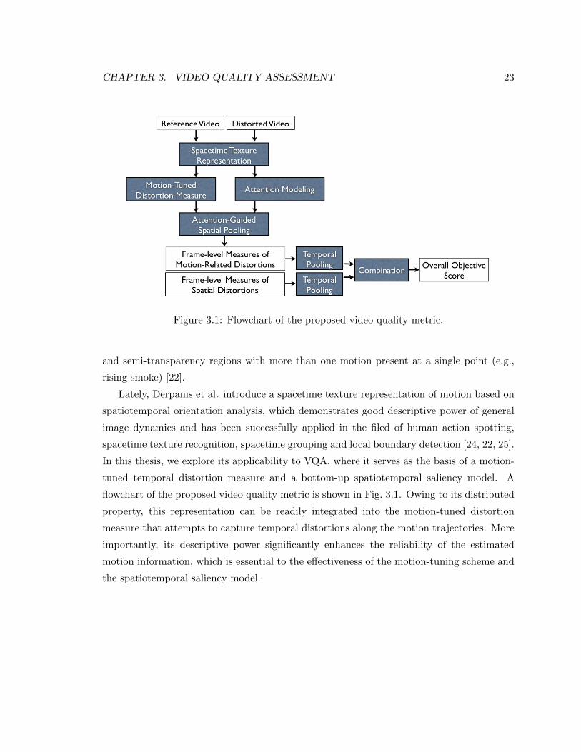
Figure 3.1: Flowchart of the proposed video quality metric.
and semi-transparency regions with more than one motion present at a single point (e.g.,
rising smoke) [22].
Lately, Derpanis et al. introduce a spacetime texture representation of motion based on
spatiotemporal orientation analysis, which demonstrates good descriptive power of general
image dynamics and has been successfully applied in the filed of human action spotting,
spacetime texture recognition, spacetime grouping and local boundary detection [24, 22, 25].
In this thesis, we explore its applicability to VQA, where it serves as the basis of a motion-
tuned temporal distortion measure and a bottom-up spatiotemporal saliency model. A
flowchart of the proposed video quality metric is shown in Fig. 3.1. Owing to its distributed
property, this representation can be readily integrated into the motion-tuned distortion
measure that attempts to capture temporal distortions along the motion trajectories. More
importantly, its descriptive power significantly enhances the reliability of the estimated
motion information, which is essential to the effectiveness of the motion-tuning scheme and
the spatiotemporal saliency model.

CHAPTER 3. VIDEO QUALITY ASSESSMENT 24
3.2 Related work
3.2.1 Motion modeling based VQA methods
Methods that explicitly incorporate motion estimation for video quality assessment are
referred to as “motion modeling based methods”. As motion plays an important role in
affecting the perceptual video quality, the incorporation of motion models represents a
significant step forward to the ultimate goal of objective VQA – matching human judgment
of video quality [9].
In the early work, motion information is employed to estimate the weights for pooling the
local quality measures into a single quality score. Wang et al. [83] propose a VQA algorithm
based on the SSIM index [80]. Firstly, intra-frame SSIM scores are obtained for each frame in
the video. Then, they use a block matching based motion estimation algorithm to evaluate
the motion in each frame, with respect to its adjacent next frame. At last, a weighted average
of the intra-frame SSIM scores are used to indicate the overall video quality, in which the
frames with large global motion are given less weights based on the assumption that spatial
distortions (such as blurring) are less annoying when the background of the video is moving
very fast. Later, they propose a more sophisticated method for video quality assessment
based on a statistical model of human visual speed perception [81]. The motion information
in their method is obtained using Black and Anandan’s multi-layer optical flow estimation
algorithm [6]. Specifically, they define the relative motion at each location as the vector
difference between the absolute motion and the global motion, ~vr = ~va− ~vg. And the speed
of motion is defined as the length of the motion vector v = ||~v||. They suggest that the
motion information content I increases with the speed of relative motion vr: I = α log vr+β,
where α and β are constants. In addition, they define a perceptual uncertainty measure, U ,
of the information received, as a function of the global motion and the stimulus contrast,
in which they assume that the uncertainty increases with global motion and decreases with
contrast. After that, the local weights w = I − U are computed at each spatiotemporal
location to combine the SSIM-based local quality measures into an overall quality score.
Moorthy et al. [52] proposed a motion compensated SSIM index for video quality as-
sessment. In the reference video, each local image patch centered at (iR, jR) in frame k is
mapped to a motion-compensated block (i′R, j′R) in frame k− 1. The displacement between
(iR, jR) and (i′R, j′R) is indicated by a motion vector, which is obtained by a block matching
method. Simialrly, in the distorted video, a motion-compensated block (i′D, j′D) for the block

CHAPTER 3. VIDEO QUALITY ASSESSMENT 25
(iD, jD) is found. Then the SSIM index is performed on the two motion-compensated blocks
to obtain a local quality measure. Another work based on motion-compensated spatial dis-
tortion measures is the TetraVQA metric developed by Barkowsky et al. [5], in which the
block matching based motion estimation is incorporated to capture the degradations that
stick to moving objects.
Seshadrinathan and Bovik [67] propose a Video Structural Similarity (V-SSIM) index
based on the similarity between the responses of motion-tuned Gabor filters to the reference
video and their responses to the test video. Given that a specific velocity in the space
domain manifests itself as a plane passing through the origin in the frequency domain [87],
the V-SSIM index uses only the filters that overlap significantly with the plane of the local
velocity in the frequency domain to calculate the similarity at that location. The motion
estimation is done by Fleet and Jepson’s phase based optical flow algorithm [30], which, as
reported in their paper, fails on some videos containing fast moving objects. Lately, they
present the MOVIE video quality index [68], which consists of a spatial quality component
and a temporal quality component. The spatial quality component is also based on an error
measure at the output of the Gabor filters between the reference video and the distorted
video. And the temporal quality component can be viewed as an extension of the V-SSIM
index – instead of selecting a subset of the Gabor filters for similarity measure, they weight
the responses of the Gabor filters based on the distances from the center frequencies of the
Gabor filters to the velocity plane in the frequency domain. The motion information is
computed by a multi-scale version of the aforementioned optical flow algorithm [30], which
achieves better robustness at the cost of considerable computation load. The MOVIE index
is reported to achieve the best quality prediction performance compared with a set of state-
of-the-art VQA methods [69].
Except for the V-SSIM index [67] and the MOVIE index [68], most of aforementioned
motion modeling based methods primarily rely on a spatial quality measure (such as the
SSIM index), where the motion information is employed as auxiliary forces, e.g., in com-
puting local weights for spatiotemporal pooling ([83, 81]) and in spatial quality evaluation
with motion compensation ([52, 5]). In other words, they do not perform direct comparison
between a reference video and a test video with respect to the dynamic attributes. On the
contrary, the V-SSIM index and the MOVIE index capture the dynamic attributes of visual
scenes by the 3D Gabor filters. Furthermore, the filter responses are tuned to the direction
of motion in an effort to capture the temporal distortions. It is worth mentioning that all

CHAPTER 3. VIDEO QUALITY ASSESSMENT 26
these motion modeling based VQA methods perform motion estimation based on block-
matching and/or optical-flow methods, which are considered to be inadequate in capturing
the general image dynamics [22].
3.2.2 Visual attention based VQA methods
Most of the attention-guided VQA methods utilize visual attention to heavily penalize dis-
tortions occurring in the highly attentional areas, where the PSNR or SSIM [80] indexes are
typically used as the local distortion measure. Bottom-up attention models based on purely
spatial cues (e.g. color, intensity and orientation) are incorporated for VQA in [29] and
[54]. In [95], semantic image analysis (face and text detection) is combined with a bottom-
up spatial saliency model to extract visual attention regions, relying on the assumption that
viewers usually pay more attention to face and text regions. More recent works often incor-
porate visual attention models with consideration for motion-driven attention [94, 48, 98, 20].
You et al. [94] develop an attention model similar to the one presented in [49] for VQA,
where the motion vectors are obtained based on a block matching method, and a spatial
window and a temporal sliding window are used in computing the spatial and temporal
coherence inductors in the attention model. Ma et al. [48] use a Quaternion Representation
(QR) for each frame, where each QR image contains one luminance channel, two motion
vector channels, and one temporal residual channel. The motion information is obtained
by a block matching method. After that, the Quaternion Fourier Transform (QFT) [27] is
employed to generate the visual saliency map. Zhu et al. [98] propose a motion-decision
based spatiotemporal model for VQA, in which they assume that motion saliency exists
if significant motion exists and it is not global motion (such as motion caused by camera
motion). In their model, an optical flow method is used to compute the motion vectors, and
then the SUN (saliency using natural statistics) model [97] is used to compute the motion
saliency under the framework of a Bayesian approach using the notation that saliency is
information. Culibrk et al. [20] use a background modeling and segmentation method [19]
to detect salient motion regions without explicit motion estimation. A major drawback of
this method is that it only applies to video sequences grabbed from a stationary camera.
Gu et al. [32] present a visual attention model by measuring two conditional probabilities
of a spatiotemporal event (i.e., a local image patch), one in its spatial context and one in
its temporal context. Though low computation complexity is achieved, its saliency estima-
tion is not as accurate as those with explicit motion modeling. There are also some other

CHAPTER 3. VIDEO QUALITY ASSESSMENT 27
VQA methods that attempt to model the interaction between attention and the spatial or
spatio-velocity contrast sensitivity of the HVS [47, 93, 92]. In spite of the theoretical value
of these methods, they demand for precise motion estimation and eye fixation prediction,
and the model parameters are often dependent on the viewing conditions.
3.3 Capturing motion-related structural distortions
3.3.1 Motion-tuned spatiotemporal oriented energies
We follow Derpanis et al.’s approach [25] to the construction of a reliable motion respresen-
tation, and meanwhile exploit its efficacy to serve our purpose, i.e., VQA. In their approach,
a video sequence is first filtered spatiotemporally using a bank of broadly tuned Gaussian
third derivative filters,
G3θ= ∂3c exp[−(x2 + y2 + t2)]/∂θ3, (3.1)
where (x, y, t) is a spatiotemporal position, θ is a unit vector that captures the spatiotempo-
ral direction of the filter symmetry axis, and c is a normalization factor. Each filter responds
best to a stimulus moving in a specific direction in the spatiotemporal space. As in [25],
the responses are pointwise rectified and summed over a spatiotemporal neighborhood (a
spatiotemporal region Π) to yield a measurement of signal energy for this region at each
orientation θ:
Eθ(x, y, t) =∑
(x,y,t)∈Π
(G3θ∗ V )2 (3.2)
where V = V (x, y, t) denotes the input video sequence, and the symbol “*” denotes convo-
lution. The bandpass nature of G3 filters leads to the invariance of the energies to additive
intensity variations. In other words, the energies are independent of the average luminance.
However, the local energy estimates still increase monotonically with contrast. In order
to capture the structural distortions irrespective of both the additive intensity variations
and contrast change, a pixelwise divisive normalization is performed. Specifically, the local
energy measures are normalized by the sum of energy responses from all filters considered
at each location,
Eθk(x, y, t) =Eθk(x, y, t)∑K
k=1Eθk(x, y, t) + ε(3.3)
where θk denote the unit vector of the k-th filter in the selected filter bank, K is the total
number of orientations/filters considered, ε is a noise floor introduced to avoid numerical

CHAPTER 3. VIDEO QUALITY ASSESSMENT 28
instabilities when the sum of energies at a point is very small.
Let Erθk
(x, y, t) and Edθk
(x, y, t) denote the normalized local energy measure in the refer-
ence video and distorted video, respectively. Now, we can obtain a local structural distortion
measure at each location (x, y, z) by calculating the similarity between the two corresponding
energy distributions in the reference and distorted videos. There are a variety of measures
that can be used to measure the similarity between two distributions [64]. In this paper, we
use the efficient L2 distance:
SD(x, y, t) = [K∑k=1
(Erθk
(x, y, t)− Edθk
(x, y, t))2]1/2. (3.4)
In this measure, each filter in the selected filter bank plays an equally important part.
However, it has been shown that measuring distortion along the motion trajectories can
better capture the temporal distortions [67, 68]. Inspired by their work, we propose a motion-
tuned structural distortion measure by assigning biased weights to the filters based on the
local motion patterns. Following the method in [25], a distributed motion representation can
be efficiently computed by “appearance marginalization” of the oriented energies in Eq. 3.2.
The goal of this marginalization is to capture the purely dynamic properties of a scene, i.e.,
the motion-related properties independent from the spatial appearance. As a pattern with a
specific velocity manifests itself as a plane through the origin in the frequency domain [87],
the purely spatial orientation component in Eq. 3.2 can be discounted by summation across
a set of spatiotemporal oriented energy measurements consistent with the corresponding
frequency plane. Let a frequency plane be parameterized by its unit normal n, and N the
order of the Gaussian filters (here, N = 3). On each plane, N + 1 equally spaced directions
{θj , j = 1, . . . , N + 1} are sampled for summation,
En =
N+1∑j=1
Eθj , (3.5)
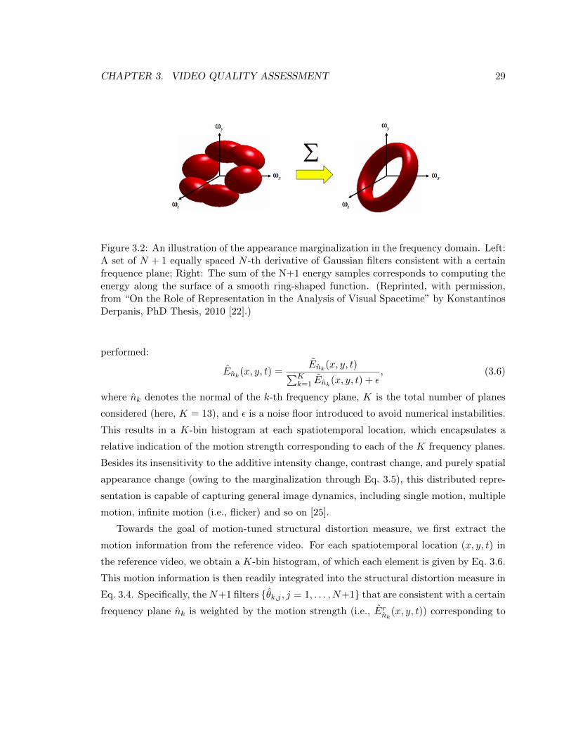
with each Eθj being the spatiotemporal energy (Eq. 3.2) at the orientation θj (see 3.2). In
this study, 13 different directions (i.e., n) are selected, corresponding to static (no motion),
motion in eight directions (leftward, rightward, upward, downward and the four diagonals),
and flicker in four directions (horizontal, vertical and two diagonals). An illustration of the
appearance marginalization is given in Fig. 3.2.
To attain insensitivity to contrast change, a divisive normalization similar to Eq. 3.3 is
CHAPTER 3. VIDEO QUALITY ASSESSMENT 29
Figure 3.2: An illustration of the appearance marginalization in the frequency domain. Left:A set of N + 1 equally spaced N -th derivative of Gaussian filters consistent with a certainfrequence plane; Right: The sum of the N+1 energy samples corresponds to computing theenergy along the surface of a smooth ring-shaped function. (Reprinted, with permission,from “On the Role of Representation in the Analysis of Visual Spacetime” by KonstantinosDerpanis, PhD Thesis, 2010 [22].)
performed:
Enk(x, y, t) =Enk(x, y, t)∑K
k=1 Enk(x, y, t) + ε, (3.6)
where nk denotes the normal of the k-th frequency plane, K is the total number of planes
considered (here, K = 13), and ε is a noise floor introduced to avoid numerical instabilities.
This results in a K-bin histogram at each spatiotemporal location, which encapsulates a
relative indication of the motion strength corresponding to each of the K frequency planes.
Besides its insensitivity to the additive intensity change, contrast change, and purely spatial
appearance change (owing to the marginalization through Eq. 3.5), this distributed repre-
sentation is capable of capturing general image dynamics, including single motion, multiple
motion, infinite motion (i.e., flicker) and so on [25].
Towards the goal of motion-tuned structural distortion measure, we first extract the
motion information from the reference video. For each spatiotemporal location (x, y, t) in
the reference video, we obtain a K-bin histogram, of which each element is given by Eq. 3.6.
This motion information is then readily integrated into the structural distortion measure in
Eq. 3.4. Specifically, theN+1 filters {θk,j , j = 1, . . . , N+1} that are consistent with a certain
frequency plane nk is weighted by the motion strength (i.e., Ernk(x, y, t)) corresponding to

CHAPTER 3. VIDEO QUALITY ASSESSMENT 30
this plane. This leads to a motion-tuned structural distortion measure:
MT -SD(x, y, t) = [K∑k=1
Ernk(x, y, t)×N+1∑j=1
(Erθk,j
(x, y, t)− Edθk,j
(x, y, t))2]1/2, (3.7)
where Erθk,j
(x, y, t) and Edθk,j
(x, y, t) are the energy responses (see Eq. 3.3) from the G3 filter
at orientation θk,j in the reference video and the distorted video, respectively.
Now we compare the proposed motion-tuned structural distortion measure with the tem-
poral component of the MOVIE index [68], as they are both based on the weighted error of
the rectified filter responses between the reference video and the test video. The MOVIE in-
dex first computes motion vectors for the pixels in the reference video based on a multi-scale
optical flow algorithm, which, as reported in their paper, does not produce flow estimates for
every pixel due to the lack of information for motion estimation in some places. As a result,
the motion-tuning scheme is inactive in these places. For a pixel associated with a velocity
estimate, it first finds the corresponding plane in the frequency domain. Then the distances
from the center frequencies of the Gabor filters to this plane are calculated. The filters lying
close to the plane are heavily weighted in calculating the motion tuned energies at each
point, where the weighted rectified filter responses are summed up over all filters, followed
by a normalization step. Given that it is often difficult to attain precise velocity estimates
using an optical flow algorithm, the frequency planes computed from the velocity estimates
are not reliable. This inevitably affects the effectiveness of the motion-tuning scheme, since
the weight for a Gabor filter could be calculated based on its distance to a wrong plane (not
corresponding to the true velocity at this pixel) in the frequency domain. More importantly,
the assumption of a single pointwise velocity is often too restrictive for describing natural
scenes. For instance, multiple image velocities are present at a single image point in a semi-
transparency scene (e.g., rising smoke). And in a campfire scene, the fire region consists of
pure temporal variation (flicker/infinite motion) [22]. Therefore, the motion-tuning scheme
of the MOVIE index is not robust in these situations. On the contrary, the distributed
motion representation employed in the proposed method exhibits much better descriptive
power in modeling complex image dynamics [22, 25]. In addition, the motion information
is efficiently incorporated into the motion-tuning cheme, which saves considerable amount
of time on estimating the motion vectors through iterative optimization, as well as on the
intensive computation of the filter-to-plane distance for each filter at each pixel.

CHAPTER 3. VIDEO QUALITY ASSESSMENT 31
3.3.2 Self-information based bottom-up spatiotemporal saliency
Bruce and Tsotsos propose the Attention by Information Maximization (AIM) principle
for visual saliency modeling, which advocates that saliency computation should serve to
maximize information sampled from one’s environment from a stimulus driven perspec-
tive [10, 11, 12]. In [11], image saliency is computed based on the Shannon’s self-information
of each local image patch given its surround, in which each image patch is coded based on
an independent component analysis (ICA) [77]. In our previous work [58], we have explored
the applicability of this image saliency model to IQA with some success. In [12], the saliency
model is extended to the spatiotemporal domain, using a set of spatiotemporal ICA bases.
In this study, we apply the AIM principle to model the spatiotemporal visual saliency for
VQA.
Three saliency models are investigated: the first one is based on the self-information
of the motion descriptors Enk(x, y, t) (see Eq. 3.6); the second one is based on the self-
information of the intermediate local motion descriptors Enk(x, y, t) (see Eq. 3.5); and
the last one is a combination of these two. Specifically, the self-information based on the
Enk(x, y, t) is computed as follow:
SIM (x, y, t) =K∑k=1
−log(p(Enk(x, y, t))), (3.8)
where the probability p(Enk(x, y, t)) is estimated by an histogram density estimation over
all the pixels in the current frame. This model detects the regions with motion patterns that
are very different from their surround. Note that it is purely based on motion information,
and is invariant to local luminance contrast. Similarly, we compute the self-information of
Enk(x, y, t) as:
SIMC(x, y, t) =K∑k=1
−log(p(Enk(x, y, t))), (3.9)
where p(Enk(x, y, t)) is also computed based on a histogram density estimation in each
frame. Clearly, the SIMC is confounded of motion saliency and luminance contrast. The
third model is a combination of SIM and SIMC . How to combine saliency maps driven
by multiple cues remains an open problem. A general principle is that, salient motion
always attracts visual attention. If salient motion does not exist, static features should be
considered [35, 98, 50, 41]. Therefore, we compute the combined saliency as
SICOM (x, y, t) = γ · SIM (x, y, t) + (1− γ) · SIMC(x, y, t) · SIM (x, y, t), (3.10)
CHAPTER 3. VIDEO QUALITY ASSESSMENT 32
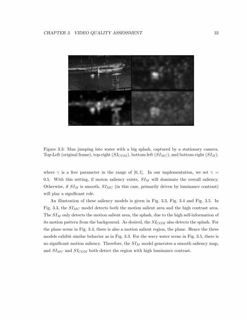
Figure 3.3: Man jumping into water with a big splash, captured by a stationary camera.Top-Left (original frame), top-right (SICOM ), bottom-left (SIMC), and bottom-right (SIM ).
where γ is a free parameter in the range of [0, 1]. In our implementation, we set γ =
0.5. With this setting, if moton saliency exists, SIM will dominate the overall saliency.
Otherwise, if SIM is smooth, SIMC (in this case, primarily driven by luminance contrast)
will play a significant role.
An illustration of these saliency models is given in Fig. 3.3, Fig. 3.4 and Fig. 3.5. In
Fig. 3.3, the SIMC model detects both the motion salient area and the high contrast area.
The SIM only detects the motion salient area, the splash, due to the high self-information of
its motion pattern from the backgournd. As desired, the SICOM also detects the splash. For
the plane scene in Fig. 3.4, there is also a motion salient region, the plane. Hence the three
models exhibit similar behavior as in Fig. 3.3. For the wavy water scene in Fig. 3.5, there is
no significant motion saliency. Therefore, the SIM model generates a smooth saliency map,
and SIMC and SICOM both detect the region with high luminance contrast.

CHAPTER 3. VIDEO QUALITY ASSESSMENT 33
Figure 3.4: Moving camera tracking a plane. Top-Left (original frame), top-right (SICOM ),bottom-left (SIMC), and bottom-right (SIM ).
3.3.3 Attention-guided spatial pooling
Based on the saliency models proposed in Section 3.3.2, we preform an attention-guided
spatial pooling to obtain a single score of the distortion level for each frame. One of the
common issues in visual attention modeling is the center-bias effect, which means that a
majority of eye fixations happen to be near the image center. This could be resulted from
the tendency of photographers to put interesting objects in the image center, or the tendency
of viewers to inspect the image center first [8]. In our implementation, we take into account
the center bias by combining a bottom-up saliency map SI with a center-bias map:
A(x, y, t) = SI(x, y, t) · CB(x, y), (3.11)
where CB(x, y) is a decreasing function of the distance between the image center and the
spatial position (x, y), and SI is chosen to be the spatiotemporal saliency model, SICOM ,
developed in Section 3.3.2. The attention-guided motion-tuned structural distortion measure

CHAPTER 3. VIDEO QUALITY ASSESSMENT 34
Figure 3.5: Wavy water with high contrast area, captured by a stationary camera. Top-Left(original frame), top-right (SICOM ), bottom-left (SIMC), and bottom-right (SIM ).
at each frame is computed as
AG-MT -SD(t) =
∑Wx=1
∑Hy=1MT -SD(x, y, t) ·A(x, y, t)∑W
x=1
∑Hy=1A(x, y, t)
, (3.12)
where [W,H] is the frame size. Under this pooling scheme, the structural distortions in
the highly attentional regions are more heavily penalized than those in the low attentional
regions.
3.4 Overall video quality prediction
3.4.1 Temporal variations of video quality
Temporal pooling concerns how people combine all the transient quality perception along
the temporal dimension into a final judgment of visual quality. A simple implementation is
to average all of them along the temporal dimension. However, it is shown that the overall
perceptual quality decreases as the temporal variation of quality along a video sequence
increases [53]. In this work, we propose a temporal pooling scheme similar to the one in [53]

CHAPTER 3. VIDEO QUALITY ASSESSMENT 35
by taking into account the temporal variations of the frame-level quality. Let D be the mean
of the per-frame distortion levels, and ∆D the standard deviation. The final distortion score
D is computed as
D =
{D + λ1∆D if λ1∆D ≤ λ2D,
D + λ2D if λ1∆D > λ2D,(3.13)
where λ1 is a scale factor that controls the influence of temporal variation, and λ2 parame-
terizes the saturation effect that limits the influence of too high temporal variations. In our
implementation, we empirically set λ1 = 1.5 and λ2 = 0.5.
3.4.2 Incorporating spatial quality
So far, we have completed the construction of a measure for structural distortions in video.
Its major properties are as follow:
• It is insensitive to luminance shift (owing the bandpass nature of the G3 filters) and
contrast change (owing to the divisive normalization).
• It primarily captures the motion-related distortions (owing to the selection of G3 filters
and the motion-tuned filtering).
• It is biased towards the salient regions (owing to the saliency-guided spatial pooling).
Clearly, the proposed structural distortion measure alone is not sufficient to give a com-
prehensive judgment of video quality, as spatial distortions also play an important part in
affecting the perceived video quality. To this end, we combine the structural distortion
measure with a spatial distortion measure:
Doverall = DMS-SSIM ·DAG-MT -SD, (3.14)
where
DMS-SSIM = 1− 1
L
L∑t=1
MS-SSIM(t) (3.15)
and
DAG-MT -SD =1
L
L∑t=1
AG-MT -SD(t). (3.16)
The MS-SSIM(t) in Eq. 3.15 is the MS-SSIM score of the t-th frame (see Eq. 2.9). Note
that each MS-SSIM score is a quality measure (i.e., high value indicates high quality) in

CHAPTER 3. VIDEO QUALITY ASSESSMENT 36
the range of [0, 1]. Therefore, the quality measure QMS-SSIM = 1L
∑Lt=1MS-SSIM(t)
is converted to a distortion measure DMS-SSIM = 1 − QMS-SSIM before calculating the
product in Eq. 3.14. The per-frame AG-MT -SD(t) score is given in Eq. 3.12. And L is the
total number of frames in a video. For simplicity, in Eq. 3.15 and Eq. 3.16, we have not
explicitly used additive terms to account for the temporal variation of quality. However,
during the evaluation, DMS-SSIM and DAG-MT -SD are adjusted according to Eq. 3.13 before
calculating the product in Eq. 3.14.
Here, the MS-SSIM index is selected because it is a widely recognized IQA metric that
has shown good effectiveness in measuring a variety of spatial distortions besides its high
computational efficiency. Since the MS-SSIM index is performed on a frame-by-frame basis,
the DMS-SSIM component primarily captures the spatial distortions as desired. In addition,
the two components are complementary in that, while the DAG-MT -SD is insensitive to
changes in luminance and contrast, the DMS-SSIM component has explicitly taken them
into account [85].
3.5 Evaluation
3.5.1 Datasets
There are two commonly used public video quality databases, namely, the VQEG FRTV
Phase 1 database [2] and the LIVE video quality database [69, 70]. The former was published
in 2000, and the distortions in the test videos (e.g., MPEG-2 and H.263 compression) are
considered to be outdated. Moreover, it spans narrow ranges of quality scores – more than
half of the test videos are of very high quality, which makes it difficult to distinguish the
performance of VQA algorithms [70]. On the contrary, the LIVE video quality database
was published in 2010, and it contains videos compressed by H.264 and MPEG-2, as well
as videos obtained by simulated transmission of H.264 compressed streams through error
prone IP and wireless networks. Besides, it spans a much wider range of quality, where the
low quality videos were designed to be of similar quality found in online video applications
(e.g. Youtube) [70]. As a result, we evaluate the proposed video quality metric on the LIVE
video quality database.

CHAPTER 3. VIDEO QUALITY ASSESSMENT 37
3.5.2 Quality prediction performance
The four metrics describe in 2.4.2 are used as performance criteria to compare difference
VQA algorithms. The performance for each component of the proposed method is shown
Table 3.1. The meanings of the notations at each row are as follow:
• “SD” – The structural distortion measure based on Eq. 3.4;
• “MT-SD” – The motion-tuned structural distortion measure based on Eq. 3.7;
• “AG-MT-SD” – The attention-guided structural distortion measure based on Eq. 3.12;
• “MS-SSIM” – The mean of frame-level MS-SSIM [85] scores;
• “Proposed Overall” – the overall quality prediction based on Eq. 3.14.
Besides, the suffix “(tv)” indicates that the temporal variation of quality is taken into
account by applying Eq. 3.13.
We can see that the “MT-SD” metric achieves significant performance gain over the
“SD” metric, which supports the effectiveness of the proposed motion tuning scheme. More-
over, the spatiotemporal saliency based weighting in the “AG-MT-SD” metric significantly
improves the “MT-SD” metric, which indicates that the proposed saliency model is very ef-
fective in identifying the perceptually important regions with respect to quality assessment.
For both the “AG-MT-SD” and “MS-SSIM” method, taking into account the temporal
variation of quality leads to some performance gain. This indicates that a good temporal
pooling scheme could play a beneficial role in video quality prediction. In addition, the
overall quality prediction performs significantly better than its two components (“MS-SSIM
(tv)” and “AG-MT-SD (tv)”). This supports that the MS-SSIM based metric is a good
complement of the proposed structural distortion measure.
To better demonstrate the effectiveness of the proposed method, we compare it with a
set of existing VQA algorithms, which include:
• PSNR – It is the traditional Peak Signal-to-Noise Ratio (PSNR) method, which is
often used as a baseline algorithm for IQA and VQA.
• SSIM [80] and MS-SSIM [85] – They are the means of the frame-level SSIM or MS-
SSIM scores. More information about these methods can be found in see Section 2.2.

CHAPTER 3. VIDEO QUALITY ASSESSMENT 38
Table 3.1: Performance of the proposed methods on the LIVE video quality database
Metrics SRCC KRCC PLCC RMSE
SD 0.7011 0.5087 0.7116 7.71MT-SD 0.7432 0.5529 0.7478 7.29
AG-MT-SD 0.7736 0.5806 0.7777 6.90AG-MT-SD(tv) 0.7914 0.5987 0.7933 6.68
MS-SSIM 0.7367 0.5514 0.7441 7.34MS-SSIM(tv) 0.7536 0.5640 0.7647 7.07
Proposed Overall (tv) 0.8215 0.6304 0.8274 6.16
• VSNR [13] – It is the mean of the frame-level Visual Signal to Noise Ratio (VSNR)
scores. The VSNR method proposed by Chandler and Hemami operates in two stages.
The first stage determines whether the distortion in a distorted image is visible via
wavelet-based models of visual masking and visual summation. If the distortion is
above a detection threshold, a second stage is applied, where the amount of distortion
is computed in the distortion-contrast space of multi-scale wavelet decomposition.
• V-VIF [71] – It is a visual information fidelity approach to VQA proposed by Sheikh
and Bovik, which extends their previous work for IQA, the VIF metric [72]. The
model is based on two mutual information quantities. One is the mutual information
between the input and the output of the HVS channel for the reference signal (when
no distortion is presents), and the other is the mutual information between the input
of the distortion channel and the output of the HVS channel for the test signal (when
a distortion channel exists between the signal source and the HVS). The model does
not directly deal with motion representation.
• VQM [60] – It is a popular feature-based VQA metric that extracts seven features
from the reference and test video. It does not directly deal with motion representation.
More information about this method can be found in Section 1.1.
• Speed SSIM [81] – It is a motion modeling based VQA algorithm, which uses a statis-
tical visual speed perception model to compute the weights for spatial pooling of the
SSIM maps. The speed information is obtained by a simple block matching method.
More information about this method can be found in Section 3.2.

CHAPTER 3. VIDEO QUALITY ASSESSMENT 39
• MOVIE [68] – It is the state-of-the-art motion modelling based VQA algorithm, which
attempts to capture temporal distortions along motion trajectories based on an optical
flow motion representation. More information about this method can be found in
Section 3.2.
The performances of these metrics are obtained from Seshadrinathan et al’s recent paper [69],
which conducts a comparative study of the existing VQA algorithms using the LIVE video
quality database. As the four performance metrics usually show similar patterns, we choose
to present two of them, the SRCC and PLCC, one for prediction monotonicity and one for
prediction accuracy.
In Fig. 3.6, the performances of all the VQA algorithms on the entire LIVE video quality
database are presented. We can see that among all the evaluated algorithms, the proposed
method achieves the best performance, followed by the state-of-the-art MOVIE index. This
strongly supports the effectiveness of the proposed method in matching the human percep-
tion of video quality. The MS-SSIM index also performs reasonably well, which is part of
the reason why it can serve as a good complement to the proposed structural distoriton
measure. All other methods achieve relatively poor performance. And it is no surprise that
the PSNR method achieves the worst performance among all methods evaluated.
3.5.3 Computational efficiency
When evaluating a 10-second 25 fps 432 × 768 test video on a Linux machine with an
Intel Core i2 CPU (2.33 GHz ) and 8 GB memory, the proposed method took 178 seconds
(about 3 minutes) to make a prediction, in which calculating the DAG-MT -SD component
took about 26 seconds, and calculating the DMS-SSIM component took about 152 seconds.1
In contrast, its main competitor, the MOVIE index [70], took 21150 seconds (about 5.88
hours) to evaluate the same video on the same machine, where about 37.9% of the time were
spent on filtering the videos with the Gabor filters at multiple scales, 55.7% on computing
the optical flows based on the multi-scale version of the Fleet and Jepson algorithm [30]
1The proposed method was implemented in MATLAB. Before computing the DAG-MT -SD component,the video sequences are spatially down-sampled to a coarser scale (144 × 256), and then divided into non-overlapping chunks, with each chunk containing 13 frames. Each G3 filter that spans a 13 × 13 × 13 spa-tiotemporal volume is centered on the 7th frame of each chunk. Note that, when the DAG-MT -SD componentwas performed at the finest/original scale, the time overhead was about 254 seconds. In the DMS-SSIM com-ponent, the MS-SSIM index [85] was performed on each frame of the video sequences, by computing theSSIM index [80] at five scales starting from the finest scale to four gradually coarser scales.
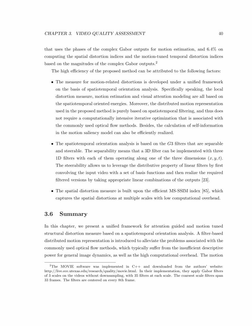
CHAPTER 3. VIDEO QUALITY ASSESSMENT 40
that uses the phases of the complex Gabor outputs for motion estimation, and 6.4% on
computing the spatial distortion indices and the motion-tuned temporal distortion indices
based on the magnitudes of the complex Gabor outputs.2
The high efficiency of the proposed method can be attributed to the following factors:
• The measure for motion-related distortions is developed under a unified framework
on the basis of spatiotemporal orientation analysis. Specifically speaking, the local
distortion measure, motion estimation and visual attention modeling are all based on
the spatiotemporal oriented energies. Moreover, the distributed motion representation
used in the proposed method is purely based on spatiotemporal filtering, and thus does
not require a computationally intensive iterative optimization that is associated with
the commonly used optical flow methods. Besides, the calculation of self-information
in the motion saliency model can also be efficiently realized.
• The spatiotemporal orientation analysis is based on the G3 filters that are separable
and steerable. The separability means that a 3D filter can be implemented with three
1D filters with each of them operating along one of the three dimensions (x, y, t).
The steerability allows us to leverage the distributive property of linear filters by first
convolving the input video with a set of basis functions and then realize the required
filtered versions by taking appropriate linear combinations of the outputs [23].
• The spatial distortion measure is built upon the efficient MS-SSIM index [85], which
captures the spatial distortions at multiple scales with low computational overhead.
3.6 Summary
In this chapter, we present a unified framework for attention guided and motion tuned
structural distortion measure based on a spatiotemporal orientation analysis. A filter-based
distributed motion representation is introduced to alleviate the problems associated with the
commonly used optical flow methods, which typically suffer from the insufficient descriptive
power for general image dynamics, as well as the high computational overhead. The motion
2The MOVIE software was implemented in C++ and downloaded from the authors’ website:http://live.ece.utexas.edu/research/quality/movie.html. In their implementation, they apply Gabor filtersof 3 scales on the videos without downsampling, with 35 filters at each scale. The coarsest scale filters span33 frames. The filters are centered on every 8th frame.

CHAPTER 3. VIDEO QUALITY ASSESSMENT 41
descriptors are then readily utilized to capture the temporal distortions along the motion
trajectories. After that, a self-information based spatiotemporal saliency model is efficiently
built based on the motion descriptors, leading to a structural distortion measure that heavily
penalizes distortions in the attention regions. At last, the proposed structural distortion
measure is combined with the MS-SSIM based spatial distortion measure to make an overall
quality prediction. The experimental results demonstrate that the proposed method has
good quality prediction ability and high computational efficiency.

CHAPTER 3. VIDEO QUALITY ASSESSMENT 42
Figure 3.6: SRCC (top) and PLCC (bottom) on the entire LVIE video quality database.
Chapter 4
Conclusions and future work
In this thesis, we propose an effective approach to amend the SSIM indexes [80, 85] with
a structural quality measure based on edge orientation analysis. We also present an ef-
fective VQA algorithm which consists of an attention-guided measure for motion-related
structural distortions based on a motion-tuned spatiotemporal orientation analysis, as well
as a measure for spatial distortions based on the MS-SSIM index [85]. Extensive evaluation
on the publicly available image/video quality databases shows that the proposed IQA and
VQA methods correlate well with the human perception of visual quality. Moreover, the
proposed methods demonstrate high computational efficiency, which will certainly enhance
their applicability in real-world applications.
The future work of this thesis lies in two directions:
• Capturing object-based image/video structure: So far, the structural informa-
tion is captured by low-level features. In our case, it is based on the spatial/spatiotemporal
orientation analysis. In the future, we will explore an objected-based definition of the
structural information. This is natural as human usually interpret a scene by first
recognizing the objects in it. For example, in the context of VQA, human often follow
the motion of objects when viewing a video [5]. It is shown that object-based video
structure can be effectively extracted through spacetime grouping and local boundary
detection based on the distributed motion representation employed in this thesis [22].
Consequently, we can measure distortion around the object boundaries, where most
of the temporal distortions occur. Moreover, the object features can also be utilized
43

CHAPTER 4. CONCLUSIONS AND FUTURE WORK 44
to model target-driven (top-down) visual attention, given that there is a consider-
able amount of evidence for target-driven attentional guidance in real world search
tasks [7].
• Along the temporal dimension: In the proposed VQA method, we have taken
into account that the variation of quality along the temporal dimension plays a ben-
eficial role in affecting the overall quality perception. However, there are many other
phenomena that occur in the temporal pooling stage of VQA, such as the forgive-
ness effect, recency effect, and negative-peak effect [57]. We believe a better temporal
pooling scheme will enhance the quality-prediction ability of the proposed method.

Bibliography
[1] Video Quality Experts Group (VQEG). http://www.its.bldrdoc.gov/vqeg/vqeg-home.aspx.
[2] VQEG FRTV Phase 1 Database. http://www.its.bldrdoc.gov/vqeg/projects/frtv-phase-i/frtv-phase-i.aspx.
[3] Recommendation ITU-R BT. 500-11. Methodology for the subjective assessment ofthe quality of television pictures. International Telecommunication Union, Geneva,Switzerland, 2002.
[4] E. Barenholtz and M.J. Tarr. Reconsidering the role of structure in vision. Psychologyof Learning and Motivation, 47:157–180, 2006.
[5] M. Barkowsky, J. Bialkowski, B. Eskofier, R. Bitto, and A. Kaup. Temporal trajectoryaware video quality measure. IEEE Journal of Selected Topics in Signal Processing,3(2):266–279, 2009.
[6] M.J. Black and P. Anandan. The robust estimation of multiple motions: Parametric andpiecewise-smooth flow fields. Computer Vision and Image Understanding, 63(1):75–104,1995-1996.
[7] A. Borji and L. Itti. State-of-the-art in visual attention modeling. IEEE Transactionson Pattern Analysis and Machine Intelligence, 35(1):185 –207, jan. 2013.
[8] A. Borji, D.N. Sihite, and L. Itti. Quantitative analysis of human-model agreement invisual saliency modeling: A comparative study. IEEE Transactions on Image Process-ing, PP(99):1, 2012.
[9] A.C. Bovik. The essential guide to video processing. Academic Press, 2009.
[10] N. Bruce and J. Tsotsos. Saliency based on information maximization. Advances inneural information processing systems, 18:155, 2006.
[11] N. Bruce and J. Tsotsos. Saliency, attention, and visual search: An information theo-retic approach. Journal of Vision, 9(3), 2009.
45

BIBLIOGRAPHY 46
[12] N. Bruce and J. Tsotsos. Spatiotemporal saliency: Towards a hierarchical representa-tion of visual saliency. Attention in Cognitive Systems, pages 98–111, 2009.
[13] D.M. Chandler and S.S. Hemami. Vsnr: A wavelet-based visual signal-to-noise ratiofor natural images. IEEE Transactions on Image Processing, 16(9):2284–2298, 2007.
[14] G. Chen, C. Yang, L. Po, and S. Xie. Edge-based structural similarity for imagequality assessment. In IEEE International Conference on Acoustics, Speech and SignalProcessing (ICASSP), volume 2, page II, may 2006.
[15] G. Chen, C. Yang, and S. Xie. Gradient-based structural similarity for image qualityassessment. In IEEE International Conference on Image Processing (ICIP), pages2929–2932, 2006.
[16] M.J. Chen and A.C. Bovik. Fast structural similarity index algorithm. Journal ofReal-Time Image Processing, 6(4):281–287, 2011.
[17] X. Chen, R. Zhang, and S. Zheng. Image quality assessment based on local edgedirection histogram. In IEEE International Conference on Image Analysis and SignalProcessing (IASP), pages 108–112, 2011.
[18] S. Chikkerur, V. Sundaram, M. Reisslein, and L.J. Karam. Objective video qualityassessment methods: A classification, review, and performance comparison. IEEETransactions on Broadcasting, 57(2):165–182, 2011.
[19] D. Culibrk, V. Crnojevic, and B. Antic. Multiscale background modelling and seg-mentation. In 16th International Conference on Digital Signal Processing, pages 1–6.IEEE, 2009.
[20] D. Culibrk, M. Mirkovic, V. Zlokolica, M. Pokric, V. Crnojevic, and D. Kukolj. Salientmotion features for video quality assessment. IEEE Transactions on Image Processing,20(4):948–958, 2011.
[21] J.G. Daugman. Uncertainty relation for resolution in space, spatial frequency, andorientation optimized by two-dimensional visual cortical filters. Journal of the OpticalSociety of America A, 2(7):1160–1169, Jul 1985.
[22] K.G. Derpanis. On the Role of Representation in the Analysis of Visual Spacetime.PhD thesis, York University, 2010.
[23] K.G. Derpanis and J.M. Gryn. Three-dimensional nth derivative of gaussian separa-ble steerable filters. In IEEE International Conference on Image Processing (ICIP),volume 3, pages III–553, 2005.
[24] K.G. Derpanis, M. Sizintsev, K. Cannons, and R.P. Wildes. Efficient action spottingbased on a spacetime oriented structure representation. In IEEE Conference on Com-puter Vision and Pattern Recognition (CVPR), pages 1990–1997, 2010.

BIBLIOGRAPHY 47
[25] K.G. Derpanis and R.P. Wildes. Spacetime texture representation and recognitionbased on a spatiotemporal orientation analysis. IEEE Transactions on Pattern Analysisand Machine Intelligence, 34(6):1193–1205, 2012.
[26] J.H. Elder and S.W. Zucker. Evidence for boundary-specific grouping. Vision Research,38(1):143–152, 1998.
[27] T.A. Ell and S.J. Sangwine. Hypercomplex fourier transforms of color images. IEEETransactions on Image Processing, 16(1):22–35, 2007.
[28] U. Engelke and H.J. Zepernick. Perceptual-based quality metrics for image and videoservices: A survey. In 3rd EuroNGI Conference on Next Generation Internet Networks,pages 190–197. IEEE, 2007.
[29] X. Feng, T. Liu, D. Yang, and Y. Wang. Saliency based objective quality assessmentof decoded video affected by packet losses. In 15th IEEE International Conference onImage Processing (ICIP), pages 2560–2563, 2008.
[30] D.J. Fleet and A.D. Jepson. Computation of component image velocity from localphase information. International Journal of Computer Vision, 5(1):77–104, 1990.
[31] X. Gao, W. Lu, D. Tao, and X. Li. Image quality assessment and human visualsystem. In Society of Photo-Optical Instrumentation Engineers (SPIE) ConferenceSeries, volume 7744, July 2010.
[32] X. Gu, G. Qiu, X. Feng, L. Debing, and C. Zhibo. Region of interest weighted poolingstrategy for video quality metric. Telecommunication Systems, 49(1):63–73, 2012.
[33] L. Cormack H.R. Sheikh, Z.Wang and A.C. Bovik. LIVE Image Quality AssessmentDatabase Release 2. http://live.ece.utexas.edu/research/quality.
[34] D.H. Hubel and T.N. Wiesel. Brain mechanisms of vision. Scientific American, 1979.
[35] L. Itti and P. Baldi. A principled approach to detecting surprising events in video.In IEEE Computer Society Conference on Computer Vision and Pattern Recognition(CVPR), volume 1, pages 631–637, 2005.
[36] J. Jain and A. Jain. Displacement measurement and its application in interframe imagecoding. IEEE Transactions on Communications, 29(12):1799–1808, 1981.
[37] T. Kadir and M. Brady. Saliency, scale and image description. International Journalof Computer Vision, 45(2):83–105, 2001.
[38] R.A. Kirsch. Computer determination of the constituent structure of biological images.Computers and Biomedical Research, 4(3):315–328, 1971.
[39] E.C. Larson and D.M. Chandler. The CSIQ Image Quality Database.http://vision.okstate.edu/?loc=csiq.

BIBLIOGRAPHY 48
[40] E.C. Larson and D.M. Chandler. Most apparent distortion: full-reference image qualityassessment and the role of strategy. Journal of Electronic Imaging, 19(1):011006–011006–21, 2010.
[41] O. Le Meur, D. Thoreau, P. Le Callet, and D. Barba. A spatio-temporal model ofthe selective human visual attention. In IEEE International Conference on ImageProcessing, volume 3, pages III–1188, 2005.
[42] K. Lee, J. Park, S. Lee, and A.C. Bovik. Temporal pooling of video quality estimatesusing perceptual motion models. In 17th IEEE International Conference on ImageProcessing (ICIP), pages 2493 –2496, sept. 2010.
[43] C. Li and A.C. Bovik. Content-partitioned structural similarity index for image qualityassessment. Signal Processing: Image Communication, 25(7):517–526, 2010.
[44] J. Li, Y. Tian, T. Huang, and W. Gao. A dataset and evaluation methodology forvisual saliency in video. In IEEE International Conference on Multimedia and Expo(ICME), pages 442–445, 2009.
[45] J. Li, Y. Tian, T. Huang, and W. Gao. Probabilistic multi-task learning for visualsaliency estimation in video. International Journal of Computer Vision, 90(2):150–165, 2010.
[46] W. Lin and C.C. Jay Kuo. Perceptual visual quality metrics: A survey. Journal ofVisual Communication and Image Representation, 22(4):297–312, 2011.
[47] Z. Lu, W. Lin, X. Yang, E.P. Ong, and S. Yao. Modeling visual attention’s modulatoryaftereffects on visual sensitivity and quality evaluation. IEEE Transactions on ImageProcessing, 14(11):1928–1942, 2005.
[48] L. Ma, S. Li, and K.N. Ngan. Motion trajectory based visual saliency for video qualityassessment. In 18th IEEE International Conference on Image Processing (ICIP), pages233–236, 2011.
[49] Y.F. Ma, L. Lu, H.J. Zhang, and M. Li. A user attention model for video summarization.In Proceedings of the 10th ACM International Conference on Multimedia (ACM MM),pages 533–542, 2002.
[50] S. Marat, T. Ho Phuoc, L. Granjon, N. Guyader, D. Pellerin, and A. Guerin-Dugue.Modelling spatio-temporal saliency to predict gaze direction for short videos. Interna-tional Journal of Computer Vision, 82(3):231–243, 2009.
[51] D. Marr and E. Hildreth. Theory of edge detection. Proceedings of the Royal Societyof London. Series B. Biological Sciences, 207(1167):187–217, 1980.
[52] A.K. Moorthy and A.C. Bovik. A motion compensated approach to video qualityassessment. In Conference Record of the Forty-Third Asilomar Conference on Signals,Systems and Computers, pages 872–875. IEEE, 2009.

BIBLIOGRAPHY 49
[53] A. Ninassi, O. Le Meur, P. Le Callet, and D. Barba. Considering temporal variations ofspatial visual distortions in video quality assessment. IEEE Journal of Selected Topicsin Signal Processing, 3(2):253–265, 2009.
[54] C. Oprea, I. Pirnog, C. Paleologu, and M. Udrea. Perceptual video quality assess-ment based on salient region detection. In Fifth Advanced International Conference onTelecommunications, pages 232–236. IEEE, 2009.
[55] J. Park, K. Seshadrinathan, S. Lee, and A.C. Bovik. Spatio-temporal quality poolingaccounting for transient severe impairments and egomotion. In 18th IEEE InternationalConference on Image Processing (ICIP), pages 2509–2512, 2011.
[56] K. Pauwels and M.M. Van Hulle. Realtime phase-based optical flow on the gpu. In IEEEComputer Society Conference on Computer Vision and Pattern Recognition Workshops(CVPRW), pages 1–8, 2008.
[57] D.E. Pearson. Viewer response to time-varying video quality. In Human Vision andElectronic Imaging III, pages 16–25. International Society for Optics and Photonics,1998.
[58] P. Peng and Z.N. Li. Self-information weighting for image quality assessment. In 4thIEEE International Congress on Image and Signal Processing (CISP), volume 4, pages1728–1732, 2011.
[59] P. Peng and Z.N. Li. Regularization of the structural similarity index based on preser-vation of edge direction. In IEEE International Conference on Systems, Man, andCybernetics (IEEE SMC), 2012.
[60] M.H. Pinson and S. Wolf. A new standardized method for objectively measuring videoquality. IEEE Transactions on Broadcasting, 50(3):312–322, 2004.
[61] N. Ponomarenko, F. Battisti, K. Egiazarian, J. Astola, and V. Lukin. Metrics per-formance comparison for color image database. In Fourth International Workshop onVideo Processing and Quality Metrics for Consumer Electronics, volume 27, 2009.
[62] N. Ponomarenko, V. Lukin, A. Zelensky, K. Egiazarian, M. Carli, and F. Battisti. TheTID Image Quality Database. http://www.ponomarenko.info/tid2008.htm.
[63] N. Ponomarenko, V. Lukin, A. Zelensky, K. Egiazarian, M. Carli, and F. Battisti.Tid2008-a database for evaluation of full-reference visual quality assessment metrics.Advances of Modern Radioelectronics, 10(10):30–45, 2009.
[64] J. Puzicha, J.M. Buhmann, Y. Rubner, and C. Tomasi. Empirical evaluation of dis-similarity measures for color and texture. In Proceedings of the 7th IEEE InternationalConference on Computer Vision (ICCV), volume 2, pages 1165–1172, 1999.

BIBLIOGRAPHY 50
[65] W. Richards and D.C. Knill. Modal structure and reliable inference. Perception asBayesian Inference, page 63, 1996.
[66] N.C. Rust, V. Mante, E.P. Simoncelli, and J.A. Movshon. How MT cells analyze themotion of visual patterns. Nature Neuroscience, 9(11):1421–1431, 2006.
[67] K. Seshadrinathan and A.C. Bovik. A structural similarity metric for video based onmotion models. In IEEE International Conference on Acoustics, Speech and SignalProcessing (ICASSP), volume 1, pages I–869, 2007.
[68] K. Seshadrinathan and A.C. Bovik. Motion tuned spatio-temporal quality assessmentof natural videos. IEEE Transactions on Image Processing, 19(2):335–350, 2010.
[69] K. Seshadrinathan, R. Soundararajan, A.C. Bovik, and L.K. Cormack. Study of subjec-tive and objective quality assessment of video. IEEE Transactions on Image Processing,19(6):1427–1441, 2010.
[70] K. Seshadrinathan, R. Soundararajan, A.C. Bovik, and L.K. Cormack. A subjectivestudy to evaluate video quality assessment algorithms. In SPIE Proceedings HumanVision and Electronic Imaging, volume 7527, 2010.
[71] H.R. Sheikh and A.C. Bovik. A visual information fidelity approach to video qualityassessment. In The First International Workshop on Video Processing and QualityMetrics for Consumer Electronics, pages 23–25, 2005.
[72] H.R. Sheikh and A.C. Bovik. Image information and visual quality. IEEE Transactionson Image Processing, 15(2):430–444, 2006.
[73] H.R. Sheikh, M.F. Sabir, and A.C. Bovik. A statistical evaluation of recent full ref-erence image quality assessment algorithms. IEEE Transactions on Image Processing,15(11):3440–3451, 2006.
[74] D. Thompson and A. Wentworth. On growth and form, 2 vols. Cambridge UniversityPress, New York. imal Physiology, 123:106–114, 1952.
[75] C.J. van den Branden Lambrecht, D.M. Costantini, G.L. Sicuranza, and M. Kunt.Quality assessment of motion rendition in video coding. IEEE Transactions on Circuitsand Systems for Video Technology, 9(5):766–782, 1999.
[76] C.J. Van den Branden Lambrecht and O. Verscheure. Perceptual quality measureusing a spatiotemporal model of the human visual system. In SPIE Proceedings of theInternational Society for Optical Engineering, pages 450–461, 1996.
[77] J.H. van Hateren and A. van der Schaaf. Independent component filters of naturalimages compared with simple cells in primary visual cortex. Proceedings of the RoyalSociety of London. Series B: Biological Sciences, 265(1394):359–366, 1998.
BIBLIOGRAPHY 51
[78] B.A. Wandell. Foundations of vision. Sinauer Associates, 1995.
[79] Z. Wang. Applications of objective image quality assessment methods [applicationscorner]. IEEE Signal Processing Magazine, 28(6):137 –142, nov. 2011.
[80] Z. Wang, A.C. Bovik, H.R. Sheikh, and E.P. Simoncelli. Image quality assessment:From error visibility to structural similarity. IEEE Transactions on Image Processing,13(4):600–612, 2004.
[81] Z. Wang and Q. Li. Video quality assessment using a statistical model of human visualspeed perception. J. Opt. Soc. Amer. A, 24(12):B61–B69, 2007.
[82] Z. Wang and Q. Li. Information content weighting for perceptual image quality assess-ment. IEEE Transactions on Image Processing, 20(5):1185–1198, 2011.
[83] Z. Wang, L. Lu, and A.C. Bovik. Video quality assessment based on structural distor-tion measurement. Signal Processing: Image Communication, 19(2):121–132, 2004.
[84] Z. Wang and X. Shang. Spatial pooling strategies for perceptual image quality assess-ment. In IEEE International Conference on Image Processing (ICIP), pages 2945–2948,2006.
[85] Z. Wang, E.P. Simoncelli, and A.C. Bovik. Multiscale structural similarity for im-age quality assessment. In IEEE Conference Record of the Thirty-Seventh AsilomarConference on Signals, Systems and Computers, volume 2, pages 1398–1402, 2003.
[86] D.H. Warren and E.R. Strelow. Electronic Spatial Sensing for the Blind: Contributionsfrom Perception, Rehabilitation, and Computer Vision. Number 99. Springer, 1985.
[87] A.B. Watson and A. Ahumada. A look at motion in the frequency domain, volume84352. National Aeronautics and Space Administration, Ames Research Center, 1983.
[88] A.B. Watson and A.J. Ahumada. Model of human visual-motion sensing. OpticalSociety of America, Journal, A: Optics and Image Science, 2:322–342, 1985.
[89] A.B. Watson, J. Hu, and J.F. McGowan. Digital video quality metric based on humanvision. Journal of Electronic imaging, 10(1):20–29, 2001.
[90] S. Winkler. Perceptual distortion metric for digital color video. In Human Vision andElectronic Imaging IV, volume 3644, pages 175–184. SPIE, 1999.
[91] A.P. Witkin and J.M. Tenenbaum. On the role of structure in vision. Human andMachine Vision, 1:481–543, 1983.
[92] J. You, T. Ebrahimi, and A. Perkis. Modeling motion visual perception for video qualityassessment. In Proceedings of the 19th ACM International Conference on Multimedia(ACM MM), pages 1293–1296, 2011.

BIBLIOGRAPHY 52
[93] J. You, T. Ebrahimi, and A. Perkis. Visual attention tuned spatio-velocity contrast sen-sitivity for video quality assessment. In IEEE International Conference on Multimediaand Expo (ICME), pages 1–6, 2011.
[94] J. You, J. Korhonen, and A. Perkis. Attention modeling for video quality assessment:balancing global quality and local quality. In IEEE International Conference on Mul-timedia and Expo (ICME), pages 914–919, 2010.
[95] J. You, A. Perkis, M.M. Hannuksela, and M. Gabbouj. Perceptual quality assessmentbased on visual attention analysis. In Proceedings of the 17th ACM International Con-ference on Multimedia (ACM MM), pages 561–564, 2009.
[96] M. Yuen and HR Wu. A survey of hybrid mc/dpcm/dct video coding distortions. Signalprocessing, 70(3):247–278, 1998.
[97] L. Zhang, M.H. Tong, T.K. Marks, H. Shan, and G.W. Cottrell. Sun: A bayesianframework for saliency using natural statistics. Journal of Vision, 8(7), 2008.
[98] Y. Zhu, N. Jacobson, H. Pan, and T. Nguyen. Motion-decision based spatiotemporalsaliency for video sequences. In IEEE International Conference on Acoustics, Speechand Signal Processing (ICASSP), pages 1333–1336, 2011.