Carbon Dioxide Emissions, Economic Growth

and the Impact of the Kyoto Protocol

Draft

Abstract

In the last two decades increasing attention has been paid to the relationship between environmental degradation and economic development. According to the Environmental Kuznets Curve (EKC) hypothesis this relationship may be described by an inverted U-curve. However, recent evidence rejects the EKC hypothesis for GHG emissions in a broad sense. In this paper we analyze the driving factors of CO2 to test the theory of the EKC in the context of environmental regulations using a static and dynamic panel data model. We consider the Kyoto Protocol and the Clean Development Mechanism (CDM). The results from this study indicate that the Kyoto obligations have a reducing effect on CO2 emissions. Keywords: Environmental Kuznets Curve, Kyoto Protocol, CDM

JEL Classification: Q54 Q56

2

1 Introduction

Carbon Dioxide Emissions (CO2) emissions are considered to have the strongest impact on

climate change among the six dominant greenhouse gases mentioned by the UNFCCC. In

2009, total global CO2 emissions amounted to 31.3 billion tonnes, an increase of almost 40%

since 1990, the base year of the Kyoto Protocol. The very large regional variation in emission

trends in 2009 resulted in a 53% share of developing countries versus 44% for industrialised

countries with mitigation targets for total greenhouse gas emissions under the Kyoto protocol.

The Annex I countries are due to cut emissions by an average of at least 5.2 percent below

1990 levels (22.5 billion tonnes) by 2008-2012. Although those countries reduced CO2

emissions by about 7 percent in 2009, a large part of the decrease was due to a drop in

economic activity in response to the crisis. Indeed, emissions could increase toward pre-

recessions levels as developed countries recover their normal economic activity levels.

Given the current policy debate and the importance of evaluating the effectiveness in terms of

emission reductions of the already established climate agreements, the main aim of this paper

is to analyze to what extent emission reduction obligations from the Kyoto Protocol and the

implementation of projects such as the Clean Development Mechanism (CDM) have an effect

on CO2 emissions. In other words, the question is whether policy instruments could lead to a

decoupling of the emission growth relationship. This question is important since one of the

main obstacles in international climate negotiations is to introduce binding emission reduction

obligations to all countries without jeopardizing the development of developing countries.

From a theoretical point of view, we base our analysis on the so-called Environmental

Kuznets Curve (EKC) theory that hypothesizes an inverse U-shaped relationship between per

capita income and environmental degradation. With increasing income per capita,

environmental degradation first rises and after reaching a maximum level of degradation, the

turning point, it starts to decline. Grossman and Krueger (1995), Holtz-Eakin and Selden

(1995) as well as Selden and Song (1994) were some of the first to find this relationship,

which was derived from the work of Kuznets (1955) on economic growth and income

inequality.

3

Among the studies that analyze the relationship between income growth and CO2 emissions1,

only a few have specifically focus on the effect of the Kyoto Protocol. To our knowledge only

Mazzanti and Musolesi (2009) studied the impact of policy events on carbon emissions. They

find that the income emission relationship is affected by policy events such as the UNFCCC

in 1992 and the Kyoto Protocol in 1997. We test this relationship by introducing modern

panel data techniques and specifically considering the endogeneity of the policy variable.

The paper is structured as follows. International climate policy is briefly described in Section

2. Section 3 discuses the measurement and sources of the data used and presents the empirical

analysis and main findings. Finally, some concluding remarks are outlined in Section 4.

2 Literature Review

2.1 Kyoto Protocol and CDM

The Kyoto Protocol was prepared by the annual meetings of the UNFCCC and adopted for

use at the 1997 meeting in Kyoto. The protocol divides the member countries into different

groups: Annex-B with GHG emissions reduction obligations and the Non-Annex-B without

emission reduction obligations. It covers the main GHGs such as CO2, which represents the

biggest share, and five other GHGs. The goal of the protocol is a reduction of GHGs by 5.3%

until 2012 compared to the countries’ emission levels in 1990. It finally entered into force in

2005 after Russia had ratified the treaty and therewith at least 55 countries, which emit at least

55% of the global GHG emissions, had ratified the treaty.

The reason for the long delay between the adoption and the entering into force of the protocol

was related to the question of which countries should have binding emission reduction

obligations and what are the estimated costs from these obligations. Further there was the

question of how to incorporate and support developing countries, which in 1997 did not

account for a big share in emissions but now do, like in the case of China which faced strong

increases in its emissions during recent years. To overcome the difficulty of how to integrate

developing countries, the Kyoto Protocol tries to enhance sustainable development among

developing countries via its flexible mechanisms, the CDM and the Joint Implementation (JI).

1 For a summary of earlier investigations refer to Appendix 1.

4

The CDM opens the possibility to fulfill a country’s GHG emission reduction obligations

with Certified Emission Reduction Units (CERs) from any other developing country which is

a member of the UNFCCC. It could be considered a back door for the developed countries to

get cheap CERs to fulfill their obligations at low cost, or even to promote sustainable

development. The CDM aims on four goals: First, it shall integrate developing countries in

the international framework on environmental regulations without putting any costly

obligations on those countries. Second, the mechanism opens new markets to those countries,

or integrates those countries into a new market, such as the international carbon market,

which trades the CERs obtained from CDM. Third, The CDM could be a tool to provide

sustainable development among poorer countries. Finally, and probably the most criticized

but also reasonable goal is, that emissions are reduced at lowest cost. The technology applied

in developed countries might be at a higher level of energy efficiency, than the technology

applied in developing countries. Therefore, it might be possible to e.g. reduce with the same

amount of money invested five times more GHG in China than in Germany.

Swinton and Sarkar (2007) analyze costs and benefits for developing countries from Kyoto

Protocol and draw a very optimistically perspective. On the one hand, developing countries

are integrated in international markets and even exhibit a comparative advantage, since they

can reduce GHG emissions at a lower unit cost. On the other hand, they can attract foreign

capital, which will create positive side effects and will lead them to a cleaner growth path.

Last but not least, the integration in international environmental law may lead to an

improvement in the developing countries institutions, which again will cause positive side

effects. Rose and Spiegel (2008) test engagement in non-economic agreements to be growth

enhancing and find that joint environmental interests do foster economic ties. They find

evidence that non-participation may lead to costs in terms of lower economic exchange in

international trade and foreign direct investment.

2.2 The Environmental Kuznets Curve Hypothesis

Since the first EKC study, presented in 1991 by Grossman and Krueger, many works relating

pollution with income have been conducted - an excellent survey of early studies can be found

in Stern (1998) - but their findings do not seem to support the EKC hypothesis in a general

way. On the contrary, the results are strongly dependent on the pollutant indicators chosen as

well as on the estimated functional form and the explanatory variables included in the

regression. An overview of the most recent literature, covering different sources for the EKC

5

hypothesis can be found in Stern (2004) and Galeotti (2007). Once more the results are

inconclusive.

Among the studies supporting the EKC hypothesis, there is a wide range of pollutant

indicators. For instance, Selden and Song (1994) considered SO2, NOx and CO emissions,

Grossman and Krueger (1995) have analysed more than ten pollutants while Holtz-Eakin and

Selden (1995) studied only CO2, Berrens et al. (1997) focused on hazardous waste, Hilton and

Levinson (1998) took into account automotive lead emissions, Kahn (1998) also considered

vehicle emissions but chose those of hydrocarbon.. Huang et al. (2008) find that especially

developing countries could exhibit an EKC. They could learn from the past and remove

environmentally harmful subsidies before entering into a heavily polluting industrial stage.

Lamla (2009) confirms an EKC for CO2 for a small sample of countries and points to the

importance to control for variables like population and technological change when analyzing

the pollution-income relationship. Dietz and Rosa (1997) apply the Impact = Population *

Affluence * Technology (IPAT) framework to control for population and technology change.

They find an inverse u-shape for CO2 emissions but most of the countries in their analysis will

never reach this high level of income (turning point). Shi (2003) confirms the results of Dietz

and Rosa (1997). Finally Mazzanti and Musolesi (2009) find that the pollution-income

relationship is affected by policy events such as the UNFCCC in 1992 and the Kyoto Protocol

in 1997. Nevertheless, the oil price shock in the 80’s and the following restructuring of the

energy-economy may also play a role.

However, in other studies, similar pollutant indicators did not confirm the EKC hypothesis.

Shafik and Bandyopadhyay (1992) did not find evidence for carbon emissions but for SO2 in

opposition to Kaufmann et al. (1998) who concluded that there is no inverted U-shaped

relation between income and atmospheric SO2 concentrations. Regarding this pollutant,

Panayotou (1997) emphasizes the role of policies and institutions in flattening the EKC. In the

study conducted by Vincent (1997) none of six pollution-income relationships estimated has

the hypothesized EKC. De Bruyn et al. (1998) found that CO2, NOx and SO2 emissions are

positively correlated with income but it is possible to abate them because of technological

progress and structural change. Unruh and Moomaw (1998) present evidence that income is

not the main variable to explain the country's emissions. Finally, Agras and Chapman (1999)

did not find significant evidence for the existence of an EKC within the range of current

incomes for energy in the presence of price and trade variables. Agras and Chapman (1999)

control for past years emissions by applying a dynamic approach and find no EKC for CO2.

6

Harbaugh et al. (2002) test the same pollutants as Grossman and Krueger (1995) but do not

find an EKC what they consider to be due to data and model specification issues. York et al.

(2003) extend the IPAT model but find no evidence for an EKC for CO2, they find rising

emissions with rising GDP but at a declining pace. Martínez-Zarzoso (2009) neither finds

evidence for an EKC for CO2 when controlling for population and technological change.

As stated by Barbier (1997) there is widespread interest on the part of academics in this

analysis and on the part of policymakers in the resulting implications for environment and

development. To analyze the shape of the pollution-income relationship is very important for

establishing public policies that target emissions reduction. If we accept the EKC hypothesis,

we could deduce that no environmental intervention is needed because economic growth will

bring together the solution for environmental problems. However we can observe that rich

countries are the main contributors to the greenhouse effect.

3 Empirical Analysis

In this section we present the empirical model and the estimation results to evaluate the EKC

hypothesis for CO2 and to test whether the Kyoto Protocol has an impact on CO2 emissions. A

modified version of the stochastically impact population affluence technology model

(STRIPAT) as used by York et al. (2003) and Martínez-Zarzoso (2009) will be estimated. We

will start the analysis with a static regression model and then compare those results to a

dynamic model.

3.1 Data

The data comes from the World Bank World Development Indicators (WDI) 2010 and covers

a panel of 213 countries from 1960 until 2009.2 For the data on CO2 emissions were referred

to the Carbon Dioxide Information Analysis Center CDIAC.3 The panel is not balanced since

e.g. the data on CO2 emissions for economies in transition is only available from 1992

onwards. The data on the ratification and the CO2 emission reduction obligations is from the

UNFCCC (2010) and data on the number of financed CDM projects by country comes from

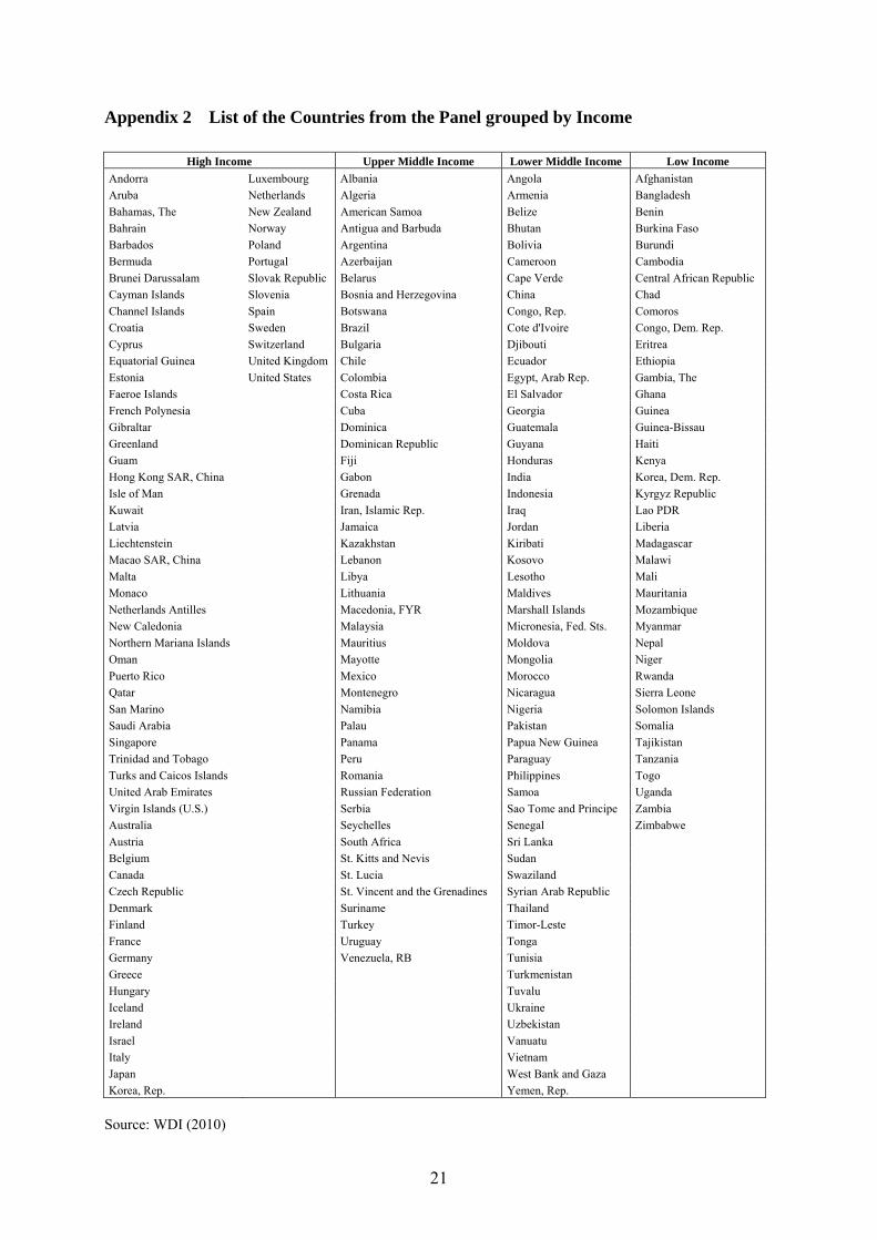
2 In an earlier version of the model we obtained our data from the WDI 2007 and came to different results in the econometrical analysis. This difference is due to the fact that some of the earlier values for GDP were revised. For a list of all the countries refer to Appendix 2. 3 The CO2 emission data includes emissions from solid, liquid as well as gas fuel consumption and emissions from cement production as well as gas flaring.

7

the UNEP Risoe Centre (2010). To analyze differences between high, middle and low income

countries we introduce dummy variables for the four groups of countries according to their

GNI.4 Emissions of CO2 are steadily increasing over the time period for the whole set of

countries. The high and upper-middle income countries emit a much higher amount of CO2

and show a stronger volatility. The low income countries emitted in 2004 about one fifth of

the amount of CO2 in kilo tons compared to the high income countries.

3.2 Model and Hypotheses

Recent macroeconomic pollution-income regressions are more general than the literature on

the EKC, not only because those include a variety of demographic and institutional variables,

but also because the elasticity of pollution with respect to emissions is allowed to differ from

unity. Following this line of research, which is also in accordance to York et al (2003), Shi,

2003 and Cole and Neumayer (2004) among others, we specify a model in which emissions

are explained with income, population, industrialization and two policy variables. This

framework is also related to the STIRPAT model that has its origin in the IPAT formulation.5

The STRIPAT model was initially proposed by Dietz and Rosa (1997):

iiiii TAPI εα δγβ= (1)

where the constant is represented by α, the parameters β, γ and δ are the coefficients which

will be estimated by the model. The error term, which represents all the unexplained variance

of the model, is denoted by ε. Finally, i stands for countries and indicates that the quantities of

A, P, T and ε vary across countries.

Dietz and Rosa (1997) include T in the error term and do not separately estimate the influence

of technology on emissions, whereas York et al. (2003) extend the model and introduce T as

another explanatory variable. By taking natural logarithms (ln) from both sides of equation 2,

we obtain

4 The grouping was done according to the WDI 2010. 5 Dietz and Rosa (1997) consider the rise in CO2 emissions to be mainly caused by human activities and apply an environmental impact model (IPAT). According to it, all impact of human activities (I) can be divided into four anthropogenic forces, which are considered to be the main driving forces behind the rise in CO2 emissions. The first one is population (P). The second is economic activity, which is referred to as affluence (A) in the model and which is measured in GDP per capita. The third is technology (T) which describes the technical standard of production and is measured in energy efficiency or industrial activity. Further determinants of CO2 are political and economic institutions as well as attitudes and beliefs.

8

iiiii TAPI µδγβα ++++= lnlnlnln 0 (2)

where α0=lnα and ii εµ ln= .

York et al. (2003) also investigate the introduction of further variables such as variables for

institutions and squared variables to measure nonlinearities in the model. They therefore lay

the foundation for the model specification, which we apply

it

ititititittiit

KyotoObIAGDPGDPGDPPCO

νββββββλα

++++++++=

6

53

42

3212 lnlnlnlnlnln (3)

where the dependent variable in (3) is CO2 Emissions measured in metric tons. iα and tλ are

country and year specific effects, which control for unobservable country-heterogeneity and

common time-varying effects that could affect emissions. Population (P) is measured in

number of inhabitants. We follow the approach of Cramer (1998) and Cramer and Cheney

(2000), who are some of the first to test whether the elasticity of emissions with respect to

population is unity.6 The variables GDP per capita and GDP per capita squared as well as

cubic represent the corner stone of the analysis for the EKC.7 The squared and cubic terms

account for possible turning points (non-linearities) of the pollution-income relationship.

Grossman and Krueger (1995) as well as Harbaugh et al. (2002) introduce this empirical

specification and find an N-shaped EKC for local pollutants.8 As a proxy for technological

change we use industrial activity (IA), calculated by the share of the manufacturing industry in

total GDP.9 We would assume countries which are specialized on agricultural production

facilities to exhibit a low share and those who are in the stage of industrialization to exhibit a

high share of manufactured goods in GDP. Developed countries in contrary might show

already a low share if they specialized in service industries.

6 In the classical approach it is assumed to be unity by using the logarithm of the pollutant in per capita terms. 7 We follow the approach of Harbaugh et al. (2002) trying to identify the right empirical specification for the EKC. 8 They further introduce three year average lagged values of GDP to account for possible dynamics. We received non-significant results on those coefficients but we will account for possible effects from past GDP on present emissions by applying a dynamic panel data model. 9 We also applied different specifications using energy efficiency as oil input per output in terms of GDP and the number registered patents as a proxy technological change. The results were neither convincing nor did they fit into the scheme of the IPAT model in the case of the later one.

9

In order to measure the impact of the Kyoto Protocol on CO2 emissions we create two

variables: The first, Kyoto obligations (KyotoOb), takes the value one, if a country has ratified

the Kyoto Protocol and faces emissions reduction obligations from the treaty, otherwise it

takes the value zero. This dummy variable takes the value one from the year on in which the

country has ratified the Kyoto Protocol. Most of the countries with emission reduction

obligations ratified the protocol in 2002. The second variable CDM accounts for the number

of CDM projects which a country has financed in countries without emission reduction

obligations to fulfill their own obligations.

The main hypotheses are:

1. Does an EKC for CO2 exist?

2. Does the variable KyotoOb have a negative effect on CO2 emissions? In other words policy

measures can have an influence on emissions.

With comparative purposes, we first estimate Equation (4) by ordinary least squares (OLS)

assuming that there is no unobserved heterogeneity across countries (αi=α) and assuming also

common slope coefficients β for all countries.10 As expected, the estimated OLS coefficients

are biased due to the existence of unobserved heterogeneity. Therefore, country specific

effects (αi) are used to model the unobserved heterogeneity between the observed countries.

We take account for those effects by estimating a random effects (RE) regression and testing

with the Lagrange Multiplier test for the significance of country specific effects. The outcome

of the test11 indicates that there are country specific effects to be taken into account.

The RE error component model assumes that the country specific effects αi are not correlated

with the independent variables xit, in other words E(xit αi)=0. If this assumption is not

fulfilled, the RE coefficients are inconsistent and the unobserved heterogeneity should be

modeled using the fixed effects (FE) estimator. The result of the Hausman test12 shows that

the RE estimator is inconsistent and, consequently, we will continue with the FE estimator,

which uses only the variation within countries over time, being less efficient than the RE but

consistent.

10 The results of the OLS regression are reported in Table 1 column (1). 11 (chi2(1) = 22617.01 and Prob > chi2 = 0.00). 12 (chi2(25) = 85.62 and Prob>chi2 = 0.00).

10

There are two further issues concerning the consistency of our model in Equation (3), which

have not been addressed so far. One is heteroscedasticity in the error term, which refers to

changes in their variance and could lead to consistent but inefficient estimates of the FE

estimator. The second one refers to serial correlation in the error term. The error term of the

current period νit could be correlated with the error term of the period before νit-1. We test for

heteroscedasticity by applying the White test for heteroscedasticity and find the error term to

be heteroscedastic.13 We further apply the Wooldridge test for autocorrelation of first order

and find that autocorrelation of order one is present in the error term14. To deal with both

problems simultaneously, heteroscedasticity and autocorrelation, a Within FE estimator with

Driscoll-Kraay standard errors is applied.15 This approach allows us to adjust the model to an

autocorrelation structure of order 1 (AR1) and heteroscedasticity (Driscoll and Kraay 1998).

Next, to test for endogeneity of right-hand-side variables we apply the Durbin Wu Hausman

test and find our KyotoOb variable to be endogenous.16 Indeed, a country with emission

reduction obligations from Kyoto Protocol will emit lower amounts of CO2 emissions, but at

the same time a country with high CO2 emissions will be more likely to face emission

reduction obligations from Kyoto Protocol. To overcome this endogeneity problem we

instrument the variable KyotoOb with the number of CDM projects which were financed by

the investing country (not by the host/implementing country) CDM. Our instrument is

correlated with the emission reduction obligations of the investing country but not with the

CO2 emissions. The first and second stages of the IV approach are

itit

ititititittiit

CDMIAGDPGDPGDPPKyotoOb

νββββββλα

++++++++=

6

53

42

321 lnlnlnlnlnln (4)

it

ititititittiit

KyotoObIAGDPGDPGDPPCO

νββββββλα

++++++++=

6

53

42

3212 lnlnlnlnlnln (5)

13 The test is applied by a regression using as dependent variable the squared error term and as independent variables all the variables in the model plus the prediction from the FE model squared and in higher exponential orders. Since the estimated coefficients for the added variables are significant, they explain some of the variance in the error term and we have to consider that the error terms is heteroscedastic. 14 (F(1,161) = 55.820 and Prob > F = 0.00). 15 The results are represented in Table 1, column (3). 16 We also apply the Hausman test and find KyotoOb to be endogenous (chi2(6) = 18.89 and Prob>chi2 = 0.00).

11

The instrumental variable approach Equation (4) and (5) accounts for the endogeneity of the

variable KyotoOb but it cannot account for heteroscedasticity or autocorrelation in the error

term and is therefore though consistent but inefficient (Baum et al. 2003).

Besides this shortcoming there is growing evidence in the literature showing that the

pollution-income relationship is a dynamic one. Agras and Chapman (1999) and Martínez-

Zarzoso (2009) are two examples. A dynamic approach assumes that today’s CO2 emissions

are driven by past ones. If a country emitted large amounts of CO2 last year, it is likely that

this year’s emissions will be high as well. The CO2 emissions of the last year therefore have

an impact on this year’s emissions. To measure this impact we introduce last year’s CO2

emissions lnCO2it-x as additional explanatory variables in the model:

itititititit

ititititittit

CDMIAGDPGDPGDP

PCOCOCOCOKyotoOb

νβββββ

βββββλα

++++++

++++++= −−−−

1093

82

76

5424323222121

lnlnlnln

lnlnlnlnlnln (6)

itit

ititititittit

KyotoObIAGDPGDPGDPPCOCO

νβββββββλα

+++++++++= −

76

35

24321212

lnlnlnlnlnlnln

(7)

The GMM IV estimator allows for an efficient estimation in the presence of heteroscedasticity

of unknown form (Baum et al. 2003). Further dynamic models suffer from a bias, which is

caused by the endogeneity of the lagged dependent variable. Since lnCO2it is a function of νit,

then lnCO2it-1 will be a function of νit as well and is therefore endogenous. The instruments Z

should be exogenous E(Zi ui)=0. The instruments yield a set of L moments equations,

( ) ⎟⎠⎞

⎜⎝⎛ −==

∧∧∧

ββ iiiiii XyZuZg ''

where gi is L x 1. The intuition of the GMM is to find the estimator, which solves ( ) 0=∧−

βg .

Therefore the instruments have to fulfill two conditions they have to be correlated with the

instrumented variables and they should not be correlated with the error terms. The Hansen

test17 yields that our instruments are valid, hence they are not correlated with the error terms.

17 (2.420 Chi-sq(3) P-val = 0.49).

12

The endogeneity test18 of the GMM IV estimator confirms that the variable KyotoOb can be

treated as endogenous.

3.3 Results

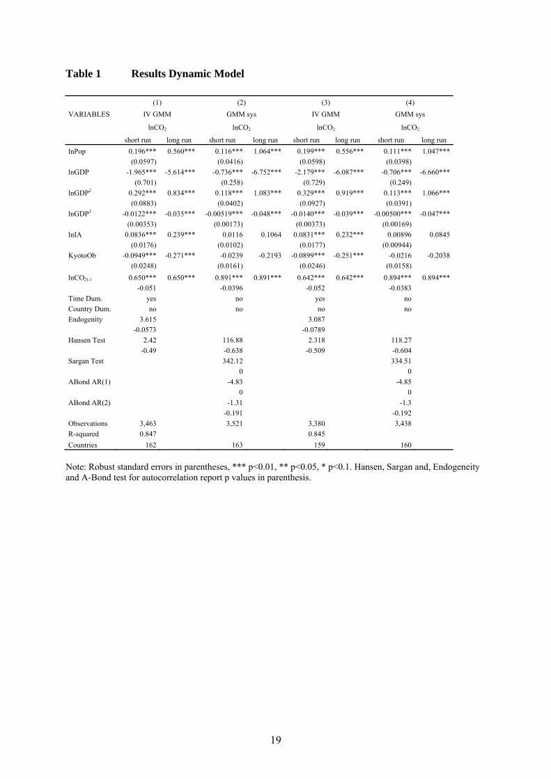
We consider the GMM IV estimator as the preferred model for our estimation and we report

the short and long run elasticities in Table 1 column (1).19 The coefficients are similar to the

ones from the IV regression in appendix 5 column (4) only the coefficient of the variable

KyotoOb has increased its magnitude and the Population variable is lower than unity. Hence a

country with emission reduction obligations from Kyoto Protocol emits on average 0.27% less

CO2 than a country without emission reductions obligations. To verify our results we also

apply the system GMM estimator by Blundell and Bond (1998) in column 2 of table 1.20

Table 1 Dynamic Results

With respect to our first hypothesis (EKC) the GDP variables indicate that emissions first

decline with rising GDP and after some turning point rise again before they decline again with

rising GDP. Instead of an inverted U-shape as in Mazzanti and Musolesi (2009) we find an

inverted N-shape. We find two turning points, a minimum at an annual average GDP per

capita of $27.38 (PPP adjusted) and a maximum of $8.52e+84. The countries in our sample

have an average GDP between $150.81 and $95434.18. Hence the turning points are clearly

out of sample and most of the countries face rising emissions with rising income.

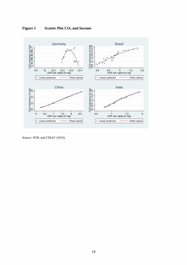
Figure 1 Scatter Plot CO2 and Income

Figure 1 displays the pollution-income relationship for four countries. Meanwhile Germany

faces declining emissions with rising income (the turning point is at $29000), Brazil, China

and India are facing strongly rising emissions with income. The graphs explain the position of

the individual countries on the inverted N-curve. Mazzanti and Musolesi (2009) do find a

cubic relationship between CO2 emissions and income. They yield insignificant income

variables when applying the cubic specification. When applying a quadratic relationship

between the variables of interest they find an inverted U-curve for the group of northern

18 (3.615 Chi-sq(1) P-val = 0.057). 19 The long-run elasticities are calculated by βxit/(1-βCO2it-1). 20 The t-value of the variable KyotoOb is -1.48 which yields that the variable is smaller than cero at 5% significance level.

13

European countries with turning points around $1300021. The different results might be due to

the grouping of the countries by Mazzanti and Musolesi (2009) and the smaller sample.

Compared to our sample they analyze mostly high and middle income countries divided in

three groups.

Concerning our second hypothesis, the variable KyotoOb has a negative effect and significant

on emissions. Hence, a country with emission reduction obligations emits on average 0.27%

less CO2 than a country without obligations.22 Mazzanti and Musolesi (2009) find as well an

effect of policy events like the Kyoto Protocol on CO2 emissions of the northern EU country

group. In fact they believe the inverted U-shape relationship between emissions and GDP is

driven by policy events such as the UNFCCC, the Kyoto Protocol and price shocks such as

the oil price shock in the eighties. In Table 1 column (3) and (4) we consider to drop three

countries with very high emission levels and without emission reduction obligations to check

if our results are robust.23The sign and significance of the estimated coefficients remain

unchanged, being the main difference that the magnitude of the effect of Kyotoob shows a

slightly lower magnitude.

Our results go in line with the literature which states that there is an EKC for some countries

(mainly high income countries which are open to environmental policies). Mazzanti and

Musolesi (2009) do mostly consider countries with emission reduction obligations from

Kyoto Protocol. We apply a potentially more comprehensive model specification of the EKC

on a larger panel of countries and contribute to the literature by controlling for the

endogeneity of the policy variables.

4 Conclusion

In this paper we analyzed and tested two relevant hypotheses. First, we examined the EKC

hypothesis for a cross-section of 163 countries over a period of 28 years. Our findings

indicate that an inverted-U relationship exists among some high-income countries such as

21 In 1995 Dollars. 22 Since most of the countries with emission reduction obligations ratified the Kyoto Protocol in 2002, we introduce interaction terms for the variable KyotoOb and the years 2001 to 2007, to see if there are year specific effects (see Table 1, column (1)and (2)). Those interaction terms turned out to be not significant in the preferred model specification and therefore are not reported. 23 The countries which were dropped are: Brazil, China and India.

14

Germany or Belgium, for middle- and low-income countries there is no evidence for future

declining emissions with rising income. The transfer of end of pipe technology could

contribute to make growth in those countries greener and avoid high emission levels, which

could cause irreversible damage.

Second, we tested for an effect of the Kyoto Protocol on CO2 emissions. We found that

countries with emission reduction obligations from Kyoto Protocol emit on average 0.27%

less CO2 than countries without obligations. Hence, there is still a long road to go and

emission reduction incentives are still too low. With respect to the flexible mechanisms of the

protocol, the CDM represents a legal tool to buy certified emission reductions (CER) from

countries without emission reduction obligations. However, it also represents a tool for

potential poverty reduction and sustainable development among middle and low income

countries.

To stabilize global warming at a 2 degrees Celsius much stronger measures will have to be

taken. A solution could try to integrate more countries in the treaty or to establish an

international taxing system on GHG emissions. After all the first commitment round of Kyoto

Protocol has just started in 2008 and we see little but some impact on global emissions from

the protocol.

15

References

Agras, J. and Chapman, D. (1999), “A Dynamic Approach to the Environmental Kuznets Curve Hypothesis”, Ecological Economics 28, 267-277.

Baiocchi, G. and di Falco, S. (2001), Investigating the Shape of the EKC - A Nonparametric Approach, Fondazione Eni Enrico Mattei, Working Paper 66.

Barbier, E.B. (1997), “Introduction to the Environmental Kuznets Curve - Special Issue”, Environment and Development Economics 2, 369-381.

Baum, C.F.; Schaffer, M.E., and Stillman, S. (2003) „Instrumental Variables and GMM - Estimation and Testing”, The Stata Journal 3, 1-31.

Bengochea-Morancho, A.; Higón-Tamarit, F. and Martínez-Zarzoso, I. (2001), “Economic Growth and CO2 Emissions in the European Union”, Environmental and Resource Economics 19, 165-172.

Berrens, R.P. et al. (1997), “Testing the Inverted-U Hypothesis for US Hazardous Waste”, Economics Letters 55, 435-440.

Blundell, R. and Bond, S. (1998), “Initial Conditions and Moment Restrictions in Dynamic Panel Data Models”, Journal of Econometrics 87, 115-143.

Cramer, J.C. (1998), “Population Growth and Air Quality in California”, Demography 35, 45-56.

Cramer, J.C. and Cheney R.P. (2000), “Lost in the Ozone – Population Growth and Ozone in California”, Population and Environment 21, 315-338.

Cole, M.A. and Neumayer, E. (2004), “Examining the Impact of Demographic Factors on Air Pollution” Population and Environment 26, 5-21.

Cole, M.A.; Rayner, A.J. and Bates, J.M. (1997), “The Environmental Kuznets Curve - An Empirical Analysis”, Environment and Development Economics 2, 401-416.

De Bruyn, S.M.; Van den Bergh, J.C. and Opschoor J.B. (1998), “Economic Growth and Emissions - Reconsidering the Empirical Basis of Environmental Kuznets Curves”, Ecological Economics 25, 161-175.

Dietz, T. and Rosa, E.A. (1997), “Effects of Population and Affluence on CO2 Emissions”, Proceedings of the National Academy of Sciences 94, 175-179.

Dijkgraaf, E. and Vollebergh, H.R.J. (2001), A Note on Testing for Environmental Kuznets Curves, Fondazione Eni Enrico Mattei, Working Paper 63.

Driscoll, J.C. and Kraay, A.C. (1998), “Consistent Covariance Matrix Estimation with Spatially Dependent Panel Data”, Review of Economics and Statistics 80, 549-560.

Ellis, J. et al. (2007), “CDM – Taking Stock and Looking Forward”, Energy Policy 35, 15-28. Fuhr, H.; Lederer, M. and Schröder, M. (2008), Neue Formen des Regierens und

Klimaschutzes durch Private Unternehmen?, GIGA Focus Global 7. Galeotti, M. (2007), “Economic Growth and the Quality of the Environment – Taking Stock”,

Environment, Development and Sustainability 9, 427-454. Galeotti, M.; Lanza, A. (1999), Richer and Cleaner? - A Study on Carbon Dioxide Emissions

in Developing Countries, Fondazione Eni Enrico Mattei, Working Paper 87. Grossman, G.M. and Krueger, A.B. (1991), Environmental Impacts of the North American

Free Trade Agreement, National Bureau of Economic Research, Working Paper 3914. Grossman, G.M. and Krueger, A.B. (1995), “Economic Growth and the Environment”, The

Quarterly Journal of Economics 110, 353-377. Harbaugh, W.T.; Levinson, A. and Molloy Wilson, D. (2002), “Reexamining the Empirical

Evidence for an Environmental Kuznets Curve”, The Review of Economics and Statistics 84, 541-551.

16

Heerink, N.; Mulatu, A. and Bulte, E. (2001), “Income Inequality and the Environment – Aggregation Bias in Environmental Kuznets Curves”, Ecological Economics 38, 359-367.

Hilton, F.G., Levinson, A. (1998), “Factoring the Environmental Kuznets Curve - Evidence from Automotive Lead Emissions.” Journal of Environmental Economics and Management 35, 126-141.

Holtz-Eakin, D. and Selden, T.M. (1995), “Stoking the Fires? CO2 Emissions and Economic Growth”, Journal of Public Economics 57, 85-101.

Huang, W.M. et al (2008), “GHG Emissions, GDP Growth and the Kyoto Protocol – A Revisit of the Environmental Kuznets Curve Hypothesis”, Energy Policy 36, 239-247.

Kahn, M.E. (1998), “A Household Level Environmental Kuznets Curve,” Economics Letters, 59, 269-73.

Kuznets, S. (1955), “Economic Growth and Income Inequality”, The American Economic Review 45, 1-28.

Lamla, M.J. (2009), “Long Run Determinants of Pollution – A Robustness Analysis”, Ecological Economics 69, 135-144.

Lecocq, F. and Ambrosi P. (2007), “The Clean Development Mechanism – History, Status and Prospects”, Review of Environmental Economics and Policy 1, 134-151.

Liu, X. (2008), “Rent Extraction with a Type-by-Type Scheme – An Instrument to Incorporate Sustainable Development into the CDM”, Energy Policy 36, 1873-1878.

Martínez-Zarzoso, I. (2009), A General Framework for Estimating Global CO2 Emissions, Ibero-America Institute for Economic Research, Discussion Paper 180.

Martínez-Zarzoso, I. and Bengochea-Morancho, A. (2004), “Pooled Mean Group Estimation of an Environmental Kuznets Curve for CO2”, Economics Letters 82, 121-126.

Martínez-Zarzoso, I.; Bengochea-Morancho, A. and Morales-Lage, R. (2007), “The Impact of Population and CO2 Emissions – Evidence from European Countries”, Environmental and Resource Economics 38, 497-512.

Mazzanti, M. and Musolesi, A. (2009), Carbon Kuznets Curves – Long-Run Structural Dynamics and Policy Events, Fondazione Eni Enrico Mattei, Working Paper 348.

Moomaw W.R. and Unruh, G.C. (1997), “Are Environmental Kuznets Curves Misleading Us? The Case of CO2 Emissions”, Environment and Development Economics 2, 451–463.

Panayotou, T. (1997): “Demystifying the Environmental Kuznets Curve - Turning a Black Box into a Policy Tool”, Environment and Development Economics 2, 465-84.

Panayotou, T.; Peterson, A. and Sachs J. (2000), Is the Environmental Kuznets Curve Driven by Structural Change? What Extended Time Series May Imply for Developing Countries, CAER II, Discussion Paper 80.

Rose, A.K. and Spiegel, M.M. (2008), Non-Economic Engagement and International Exchange – The Case of Environmental Treaties, National Bureau of Economic Research, Working Paper 13988.

Roberts, J.T. and Grimes, P.E. (1997), “Carbon Intensity and Economic Development 1962–91 - A Brief Exploration of the Environmental Kuznets Curve”, World Development 25, 191–198.

Roca J.; Padilla, E; Farré, M. and Galletto, V. (2001), “Economic Growth and Atmospheric Pollution in Spain - Discussing the Environmental Kuznets Curve Hypothesis”, Ecological Economics 39, 85–99.

Schaffer, M.E. (2010), xtivreg2: Stata module to perform extended IV/2SLS, GMM and AC/HAC, LIML and k-class regression for panel data models. http://ideas.repec.org/c/boc/bocode/s456501.html

Schmalensee, R.; Stoker, T.M. and Judson, R.A. (1998), “World Carbon Dioxide Emissions: 1950–2050”, Revenue of Economics and Statistics 80, 15–27

17

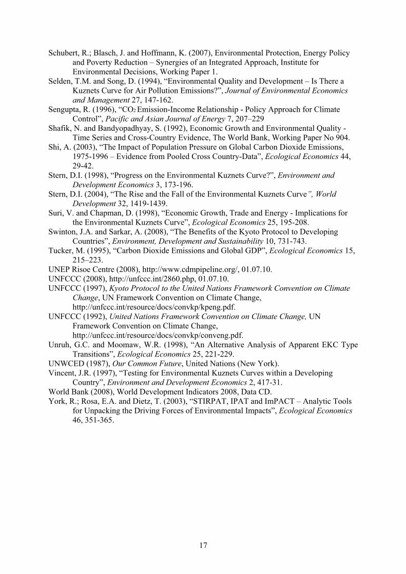
Schubert, R.; Blasch, J. and Hoffmann, K. (2007), Environmental Protection, Energy Policy and Poverty Reduction – Synergies of an Integrated Approach, Institute for Environmental Decisions, Working Paper 1.

Selden, T.M. and Song, D. (1994), “Environmental Quality and Development – Is There a Kuznets Curve for Air Pollution Emissions?”, Journal of Environmental Economics and Management 27, 147-162.

Sengupta, R. (1996), “CO2 Emission-Income Relationship - Policy Approach for Climate Control”, Pacific and Asian Journal of Energy 7, 207–229

Shafik, N. and Bandyopadhyay, S. (1992), Economic Growth and Environmental Quality - Time Series and Cross-Country Evidence, The World Bank, Working Paper No 904.

Shi, A. (2003), “The Impact of Population Pressure on Global Carbon Dioxide Emissions, 1975-1996 – Evidence from Pooled Cross Country-Data”, Ecological Economics 44, 29-42.

Stern, D.I. (1998), “Progress on the Environmental Kuznets Curve?”, Environment and Development Economics 3, 173-196.

Stern, D.I. (2004), “The Rise and the Fall of the Environmental Kuznets Curve”, World Development 32, 1419-1439.

Suri, V. and Chapman, D. (1998), “Economic Growth, Trade and Energy - Implications for the Environmental Kuznets Curve”, Ecological Economics 25, 195-208.

Swinton, J.A. and Sarkar, A. (2008), “The Benefits of the Kyoto Protocol to Developing Countries”, Environment, Development and Sustainability 10, 731-743.

Tucker, M. (1995), “Carbon Dioxide Emissions and Global GDP”, Ecological Economics 15, 215–223.

UNEP Risoe Centre (2008), http://www.cdmpipeline.org/, 01.07.10. UNFCCC (2008), http://unfccc.int/2860.php, 01.07.10. UNFCCC (1997), Kyoto Protocol to the United Nations Framework Convention on Climate

Change, UN Framework Convention on Climate Change, http://unfccc.int/resource/docs/convkp/kpeng.pdf.

UNFCCC (1992), United Nations Framework Convention on Climate Change, UN Framework Convention on Climate Change, http://unfccc.int/resource/docs/convkp/conveng.pdf.

Unruh, G.C. and Moomaw, W.R. (1998), “An Alternative Analysis of Apparent EKC Type Transitions”, Ecological Economics 25, 221-229.

UNWCED (1987), Our Common Future, United Nations (New York). Vincent, J.R. (1997), “Testing for Environmental Kuznets Curves within a Developing

Country”, Environment and Development Economics 2, 417-31. World Bank (2008), World Development Indicators 2008, Data CD. York, R.; Rosa, E.A. and Dietz, T. (2003), “STIRPAT, IPAT and ImPACT – Analytic Tools

for Unpacking the Driving Forces of Environmental Impacts”, Ecological Economics 46, 351-365.

18

Figure 1 Scatter Plot CO2 and Income 11

.511.

5511.

611.6

511.7

CO

2 em

issi

ons

(in lo

g)

9.9 10 10.1 10.2 10.3 10.4GDP per capita (in log)

Linear prediction Fitted values

Germany

10.8

1111

.211

.411

.6C

O2

emis

sion

s (in

log)

8.8 8.9 9 9.1 9.2GDP per capita (in log)

Linear prediction Fitted values

Brazil

1011

1213

CO

2 em

issi

ons

(in lo

g)

6 6.5 7 7.5 8 8.5GDP per capita (in log)

Linear prediction Fitted values

China10

10.5

1111

.512

CO

2 em

issi

ons

(in lo

g)

6.5 7 7.5 8GDP per capita (in log)

Linear prediction Fitted values

India

Source: WDI, and CDIAC (2010).

19

Table 1 Results Dynamic Model

(1) (2) (3) (4) VARIABLES IV GMM GMM sys IV GMM GMM sys

lnCO2 lnCO2 lnCO2 lnCO2

short run long run short run long run short run long run short run long run lnPop 0.196*** 0.560*** 0.116*** 1.064*** 0.199*** 0.556*** 0.111*** 1.047***

(0.0597) (0.0416) (0.0598) (0.0398) lnGDP -1.965*** -5.614*** -0.736*** -6.752*** -2.179*** -6.087*** -0.706*** -6.660***

(0.701) (0.258) (0.729) (0.249) lnGDP2 0.292*** 0.834*** 0.118*** 1.083*** 0.329*** 0.919*** 0.113*** 1.066***

(0.0883) (0.0402) (0.0927) (0.0391) lnGDP3 -0.0122*** -0.035*** -0.00519*** -0.048*** -0.0140*** -0.039*** -0.00500*** -0.047***

(0.00353) (0.00173) (0.00373) (0.00169) lnIA 0.0836*** 0.239*** 0.0116 0.1064 0.0831*** 0.232*** 0.00896 0.0845

(0.0176) (0.0102) (0.0177) (0.00944) KyotoOb -0.0949*** -0.271*** -0.0239 -0.2193 -0.0899*** -0.251*** -0.0216 -0.2038

(0.0248) (0.0161) (0.0246) (0.0158) lnCO2t-1 0.650*** 0.650*** 0.891*** 0.891*** 0.642*** 0.642*** 0.894*** 0.894***

-0.051 -0.0396 -0.052 -0.0383 Time Dum. yes no yes no Country Dum. no no no no Endogenity 3.615 3.087

-0.0573 -0.0789Hansen Test 2.42 116.88 2.318 118.27

-0.49 -0.638 -0.509 -0.604 Sargan Test 342.12 334.51

0 0 ABond AR(1) -4.83 -4.85

0 0 ABond AR(2) -1.31 -1.3

-0.191 -0.192 Observations 3,463 3,521 3,380 3,438 R-squared 0.847 0.845Countries 162 163 159 160

Note: Robust standard errors in parentheses, *** p<0.01, ** p<0.05, * p<0.1. Hansen, Sargan and, Endogeneity and A-Bond test for autocorrelation report p values in parenthesis.

20

Appendix

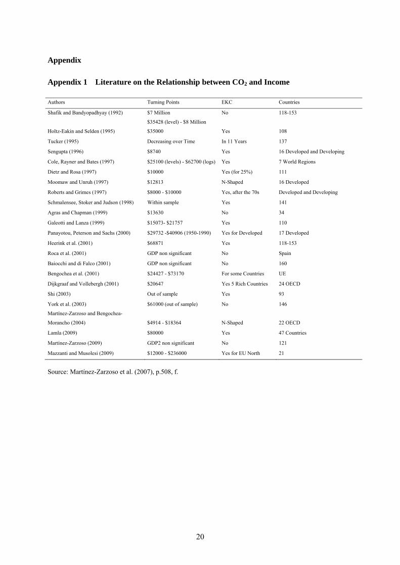
Appendix 1 Literature on the Relationship between CO2 and Income

Authors Turning Points EKC Countries

Shafik and Bandyopadhyay (1992) $7 Million No 118-153

Holtz-Eakin and Selden (1995)

$35428 (level) - $8 Million

$35000 Yes 108

Tucker (1995) Decreasing over Time In 11 Years 137

Sengupta (1996) $8740 Yes 16 Developed and Developing

Cole, Rayner and Bates (1997) $25100 (levels) - $62700 (logs) Yes 7 World Regions

Dietz and Rosa (1997) $10000 Yes (for 25%) 111

Moomaw and Unruh (1997) $12813 N-Shaped 16 Developed

Roberts and Grimes (1997) $8000 - $10000 Yes, after the 70s Developed and Developing

Schmalensee, Stoker and Judson (1998) Within sample Yes 141

Agras and Chapman (1999) $13630 No 34

Galeotti and Lanza (1999) $15073- $21757 Yes 110

Panayotou, Peterson and Sachs (2000) $29732 -$40906 (1950-1990) Yes for Developed 17 Developed

Heerink et al. (2001) $68871 Yes 118-153

Roca et al. (2001) GDP non significant No Spain

Baiocchi and di Falco (2001) GDP non significant No 160

Bengochea et al. (2001) $24427 - $73170 For some Countries UE

Dijkgraaf and Vollebergh (2001) $20647 Yes 5 Rich Countries 24 OECD

Shi (2003) Out of sample Yes 93

York et al. (2003) $61000 (out of sample) No 146

Martínez-Zarzoso and Bengochea-

Morancho (2004) $4914 - $18364 N-Shaped 22 OECD

Lamla (2009) $80000 Yes 47 Countries

Martínez-Zarzoso (2009) GDP2 non significant No 121

Mazzanti and Musolesi (2009) $12000 - $236000 Yes for EU North 21

Source: Martínez-Zarzoso et al. (2007), p.508, f.

21

Appendix 2 List of the Countries from the Panel grouped by Income

High Income Upper Middle Income Lower Middle Income Low Income Andorra Luxembourg Albania Angola Afghanistan Aruba Netherlands Algeria Armenia Bangladesh Bahamas, The New Zealand American Samoa Belize Benin Bahrain Norway Antigua and Barbuda Bhutan Burkina Faso Barbados Poland Argentina Bolivia Burundi Bermuda Portugal Azerbaijan Cameroon Cambodia Brunei Darussalam Slovak Republic Belarus Cape Verde Central African Republic Cayman Islands Slovenia Bosnia and Herzegovina China Chad Channel Islands Spain Botswana Congo, Rep. Comoros Croatia Sweden Brazil Cote d'Ivoire Congo, Dem. Rep. Cyprus Switzerland Bulgaria Djibouti Eritrea Equatorial Guinea United Kingdom Chile Ecuador Ethiopia Estonia United States Colombia Egypt, Arab Rep. Gambia, The Faeroe Islands Costa Rica El Salvador Ghana French Polynesia Cuba Georgia Guinea Gibraltar Dominica Guatemala Guinea-Bissau Greenland Dominican Republic Guyana Haiti Guam Fiji Honduras Kenya Hong Kong SAR, China Gabon India Korea, Dem. Rep. Isle of Man Grenada Indonesia Kyrgyz Republic Kuwait Iran, Islamic Rep. Iraq Lao PDR Latvia Jamaica Jordan Liberia Liechtenstein Kazakhstan Kiribati Madagascar Macao SAR, China Lebanon Kosovo Malawi Malta Libya Lesotho Mali Monaco Lithuania Maldives Mauritania Netherlands Antilles Macedonia, FYR Marshall Islands Mozambique New Caledonia Malaysia Micronesia, Fed. Sts. Myanmar Northern Mariana Islands Mauritius Moldova Nepal Oman Mayotte Mongolia Niger Puerto Rico Mexico Morocco Rwanda Qatar Montenegro Nicaragua Sierra Leone San Marino Namibia Nigeria Solomon Islands Saudi Arabia Palau Pakistan Somalia Singapore Panama Papua New Guinea Tajikistan Trinidad and Tobago Peru Paraguay Tanzania Turks and Caicos Islands Romania Philippines Togo United Arab Emirates Russian Federation Samoa Uganda Virgin Islands (U.S.) Serbia Sao Tome and Principe Zambia Australia Seychelles Senegal Zimbabwe Austria South Africa Sri Lanka Belgium St. Kitts and Nevis Sudan Canada St. Lucia Swaziland Czech Republic St. Vincent and the Grenadines Syrian Arab Republic Denmark Suriname Thailand Finland Turkey Timor-Leste France Uruguay Tonga Germany Venezuela, RB Tunisia Greece Turkmenistan Hungary Tuvalu Iceland Ukraine Ireland Uzbekistan Israel Vanuatu Italy Vietnam Japan West Bank and Gaza Korea, Rep. Yemen, Rep.

Source: WDI (2010)

22

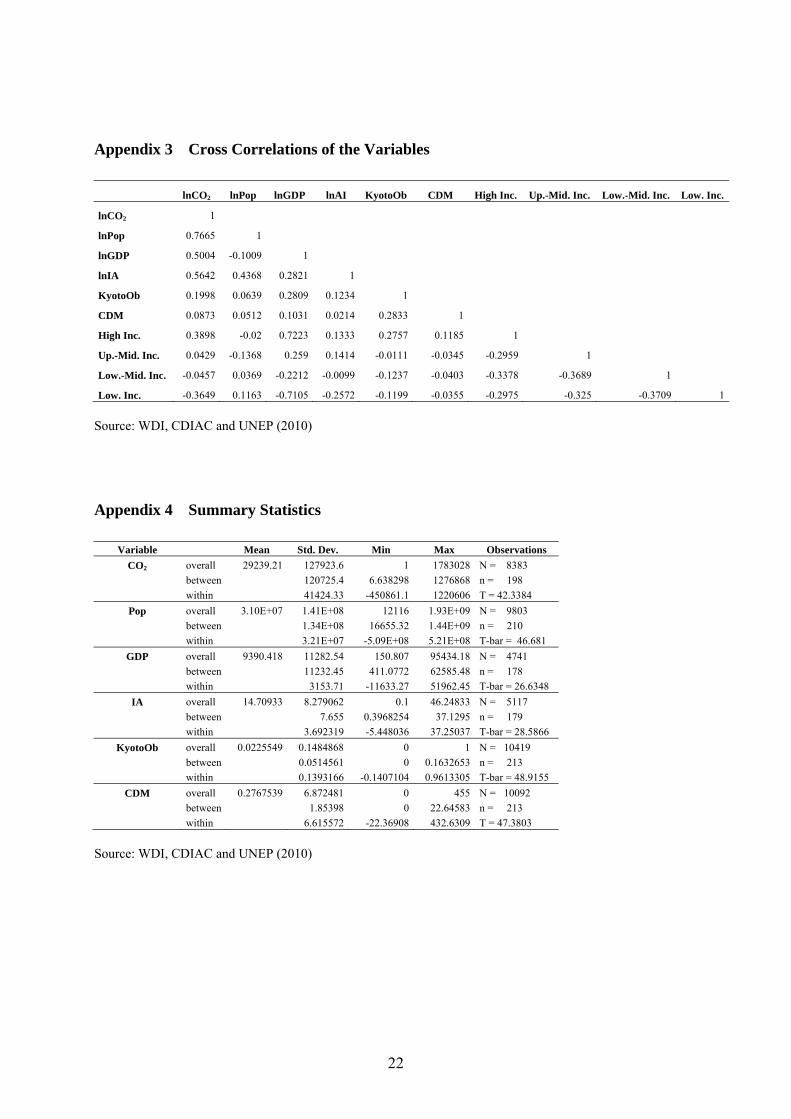
Appendix 3 Cross Correlations of the Variables

lnCO2 lnPop lnGDP lnAI KyotoOb CDM High Inc. Up.-Mid. Inc. Low.-Mid. Inc. Low. Inc.

lnCO2 1

lnPop 0.7665 1

lnGDP 0.5004 -0.1009 1

lnIA 0.5642 0.4368 0.2821 1

KyotoOb 0.1998 0.0639 0.2809 0.1234 1

CDM 0.0873 0.0512 0.1031 0.0214 0.2833 1

High Inc. 0.3898 -0.02 0.7223 0.1333 0.2757 0.1185 1

Up.-Mid. Inc. 0.0429 -0.1368 0.259 0.1414 -0.0111 -0.0345 -0.2959 1

Low.-Mid. Inc. -0.0457 0.0369 -0.2212 -0.0099 -0.1237 -0.0403 -0.3378 -0.3689 1

Low. Inc. -0.3649 0.1163 -0.7105 -0.2572 -0.1199 -0.0355 -0.2975 -0.325 -0.3709 1

Source: WDI, CDIAC and UNEP (2010)

Appendix 4 Summary Statistics

Variable Mean Std. Dev. Min Max Observations CO2 overall 29239.21 127923.6 1 1783028 N = 8383

between 120725.4 6.638298 1276868 n = 198 within 41424.33 -450861.1 1220606 T = 42.3384

Pop overall 3.10E+07 1.41E+08 12116 1.93E+09 N = 9803 between 1.34E+08 16655.32 1.44E+09 n = 210 within 3.21E+07 -5.09E+08 5.21E+08 T-bar = 46.681

GDP overall 9390.418 11282.54 150.807 95434.18 N = 4741 between 11232.45 411.0772 62585.48 n = 178 within 3153.71 -11633.27 51962.45 T-bar = 26.6348

IA overall 14.70933 8.279062 0.1 46.24833 N = 5117 between 7.655 0.3968254 37.1295 n = 179 within 3.692319 -5.448036 37.25037 T-bar = 28.5866

KyotoOb overall 0.0225549 0.1484868 0 1 N = 10419 between 0.0514561 0 0.1632653 n = 213 within 0.1393166 -0.1407104 0.9613305 T-bar = 48.9155

CDM overall 0.2767539 6.872481 0 455 N = 10092 between 1.85398 0 22.64583 n = 213

within 6.615572 -22.36908 432.6309 T = 47.3803

Source: WDI, CDIAC and UNEP (2010)

23

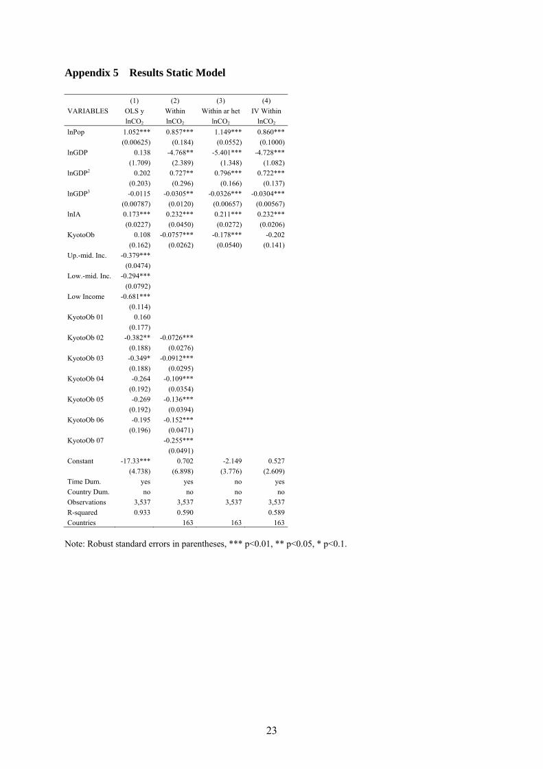
Appendix 5 Results Static Model

(1) (2) (3) (4) VARIABLES OLS y Within Within ar het IV Within lnCO2 lnCO2 lnCO2 lnCO2 lnPop 1.052*** 0.857*** 1.149*** 0.860***

(0.00625) (0.184) (0.0552) (0.1000)lnGDP 0.138 -4.768** -5.401*** -4.728***

(1.709) (2.389) (1.348) (1.082)lnGDP2 0.202 0.727** 0.796*** 0.722***

(0.203) (0.296) (0.166) (0.137)lnGDP3 -0.0115 -0.0305** -0.0326*** -0.0304***

(0.00787) (0.0120) (0.00657) (0.00567)lnIA 0.173*** 0.232*** 0.211*** 0.232***

(0.0227) (0.0450) (0.0272) (0.0206)KyotoOb 0.108 -0.0757*** -0.178*** -0.202

(0.162) (0.0262) (0.0540) (0.141)Up.-mid. Inc. -0.379***

(0.0474) Low.-mid. Inc. -0.294***

(0.0792) Low Income -0.681***

(0.114) KyotoOb 01 0.160

(0.177) KyotoOb 02 -0.382** -0.0726***

(0.188) (0.0276) KyotoOb 03 -0.349* -0.0912***

(0.188) (0.0295) KyotoOb 04 -0.264 -0.109***

(0.192) (0.0354) KyotoOb 05 -0.269 -0.136***

(0.192) (0.0394) KyotoOb 06 -0.195 -0.152***

(0.196) (0.0471) KyotoOb 07 -0.255***

(0.0491) Constant -17.33*** 0.702 -2.149 0.527

(4.738) (6.898) (3.776) (2.609)Time Dum. yes yes no yesCountry Dum. no no no noObservations 3,537 3,537 3,537 3,537R-squared 0.933 0.590 0.589Countries 163 163 163

Note: Robust standard errors in parentheses, *** p<0.01, ** p<0.05, * p<0.1.