PNNL-15239

Carbon Tetrachloride and Chloroform Partition Coefficients Derived from Aqueous Desorption of Contaminated Hanford Sediments R. G. Riley J. E. Szecsody D. S. Sklarew A. V. Mitroshkov C. F. Brown C. J. Thompson P. M. Gent July 2005 Prepared for the U.S. Department of Energy under Contract DE-AC05-76RL01830

DISCLAIMER This report was prepared as an account of work sponsored by an agency of the United States Government. Neither the United States Government nor any agency thereof, nor Battelle Memorial Institute, nor any of their employees, makes any warranty, express or implied, or assumes any legal liability or responsibility for the accuracy, completeness, or usefulness of any information, apparatus, product, or process disclosed, or represents that its use would not infringe privately owned rights. Reference herein to any specific commercial product, process, or service by trade name, trademark, manufacturer, or otherwise does not necessarily constitute or imply its endorsement, recommendation, or favoring by the United States Government or any agency thereof, or Battelle Memorial Institute. The views and opinions of authors expressed herein do not necessarily state or reflect those of the United States Government or any agency thereof.

PACIFIC NORTHWEST NATIONAL LABORATORY operated by BATTELLE

for the UNITED STATES DEPARTMENT OF ENERGY

under Contract DE-AC05-76RL01830

Printed in the United States of America

Available to DOE and DOE contractors from the Office of Scientific and Technical Information,

P.O. Box 62, Oak Ridge, TN 37831-0062; ph: (865) 576-8401 fax: (865) 576-5728

email: reports@adonis.osti.gov

Available to the public from the National Technical Information Service, U.S. Department of Commerce, 5285 Port Royal Rd., Springfield, VA 22161

ph: (800) 553-6847 fax: (703) 605-6900

email: orders@ntis.fedworld.gov online ordering: http://www.ntis.gov/ordering.htm

This document was printed on recycled paper. (8/00)

PNNL-15239

Carbon Tetrachloride and Chloroform Partition Coefficients Derived from Aqueous Desorption of Contaminated Hanford Sediments R. G. Riley J. E. Szecsody D. S. Sklarew A. V. Mitroshkov C. F. Brown C. J. Thompson P. M. Gent(a) July 2005 Prepared for the U.S. Department of Energy under Contract DE-AC05-76RL01830 Pacific Northwest National Laboratory Richland, Washington 99352 _______________

(a) Fluor Hanford, Inc.

iii

Summary

Fluor Hanford, Inc. (FHI) has identified data needs important to locating, characterizing, and assessing the impact of carbon tetrachloride (CCl4) contamination underlying the 200 West Area on the Hanford Site. One need, which is described in this report, is to establish partition coefficients between gas, liquid, and solid phases for CCl4 based on contaminated sediments and to use such data to refine the fate and transport modeling performed to assess the impacts of the 200 West Area CCl4 plume.

Researchers at PNNL determined CCl4 and chloroform (CHCl3) groundwater/sediment partition coefficients (Kd values) for contaminated aquifer sediments collected from borehole C3246 (299-W15-46) located in the 200 West Area adjacent to the 216-Z-9 trench. Having realistic values for this parameter is critical to predict future movement of CCl4 in groundwater from the 200 West Area. It is best to obtain such values from contaminated sediments because the values will reflect the long sediment/contaminant contact times that are not possible to mimic in laboratory experiments. The Kd values used in modeling CCl4 are crucial to more accurate estimation of whether compliance limits may be exceeded outside the Central Plateau waste management area.

CCl4 and CHCl3 partition coefficients for groundwater and sediment were determined in contami-nated aquifer sediments of the Ringold Formation collected at depths in the range of 230 to 430 feet from the borehole 299-W15-46. The contaminants have been in contact with these sediments for up to 30 years. CCl4 and CHCl3 partition coefficients ranged from 0.106 L/kg to 0.367 L/kg and 0.084 L/kg to 0.432 L/kg, respectively. These values were 3 to 8 times and 12 to 23 times larger, respectively, than would be predicted based on the organic carbon content of the sediments (0.017 to 0.059%).

These partition coefficients, along with groundwater concentrations of CCl4 and CHCl3 measured at the same location of sediment collection, were used to estimate sediment concentrations of CCl4. In some cases, predicted values were significantly higher than observed sediment concentrations of CCl4 (e.g., 904 µg/kg calculated versus 31.8 µg/kg observed). A likely rationale for this difference is degradation of CCl4 in the sediments. A significant fraction of CHCl3 (61% to 70% of the total solute mass) was observed to be resistive to desorption from some of the sediments. The apparent sequestering properties of these sediments suggest that a certain portion of the CHCl3 in Hanford aquifer sediments is migrating more slowly in groundwater than would be predicted by simple partitioning between groundwater and sediment.

Past modeling of the CCl4 transport in the Hanford groundwater aquifer has assumed conservative values for contaminant partitioning (e.g., a Kd value of 0 and no degradation), resulting in predictions that CCl4 concentrations will exceed compliance limits on the 200 Area plateau and at the Columbia River within a 1,000 year time frame. Use of the Kd values determined in this study in transport simulations would result in slower predicted migration rates and reduced uncertainty. The presence of significant concentrations of CHCl3 in the presence of lower-than-expected concentrations of CCl4 indicated CCl4 degradation in the sediment and the need to more accurately represent this process in transport modeling.

v

Contents

Summary ............................................................................................................................................ iii

1.0 Introduction.............................................................................................................................. 1.1

2.0 Sampling Methods ................................................................................................................... 2.1 2.1 Collection of Intact Sediment Cores............................................................................... 2.1

2.2 Conversion of Liners to Intact Core Transport Containers ............................................ 2.1

2.3 Conversion of Transport Containers into Desorption Columns ..................................... 2.3

2.4 Collection of Groundwater Samples .............................................................................. 2.3

3.0 Sample Preparation and Analysis Methodology ...................................................................... 3.1 3.1 Sediment Moisture Content............................................................................................ 3.1

3.2 Bulk Fraction Distribution Analysis............................................................................... 3.1

3.3 Carbon Analysis ............................................................................................................. 3.1

3.4 Analysis of Water Samples by Gas Chromatography/Mass Spectrometry .................... 3.2

3.5 Accelerated Solvent Extraction of Sediments ................................................................ 3.3

3.6 Analysis of Sediment Extracts by Gas Chromatography ............................................... 3.4

4.0 Experimental Desorption System and Solute Elution .............................................................. 4.1

5.0 Tracer/Solute Profile Simulations from 1-D Column Experiments ......................................... 5.1 5.1 Partition Coefficients from Profile Determination of Retardation Factors .................... 5.1

5.2 Model Simulations to Assess Tracer/Solute Behavior ................................................... 5.1

6.0 Results ...................................................................................................................................... 6.1 6.1 Physical and Chemical Characteristics of Sediment Cores ............................................ 6.1

6.2 Desorption Experiments ................................................................................................. 6.2 6.2.1 CCl4 and CCl3 Behavior in Column Desorption Experiments .......................... 6.2 6.2.2 Simulation of Tracer Behavior in 1-D Column Experiments............................ 6.6 6.2.3 Simulation of CCl4 Behavior in Column Desorption Experiments ................... 6.6 6.2.4 Simulation of Chloroform Behavior in Column Desorption Experiments........ 6.10

6.3 Carbon Tetrachloride and Chloroform Residuals in Sediment Cores ............................ 6.10

6.4 Initial Sediment Core Solute Concentrations ................................................................. 6.10

6.5 Concentrations of Solutes in Samples of Groundwater Collected at Sediment Depth Locations ............................................................................................................. 6.12

vi

6.6 Predicted Versus Observed Kd Values ........................................................................... 6.12

6.7 Predicted Versus Observed Sediment Core Solute Concentrations ............................... 6.13

7.0 Discussion ................................................................................................................................ 7.1

8.0 References ................................................................................................................................ 8.1

Appendix A – Calculation of CH Concentration from GC-MS Data

Appendix B – Column Experiment Breakthrough Data

Figures

1.1 Location of C3426 Borehole Relative to 216-Z-9 Trench.................................................... 1.2 2.1 Aquifer Sediment in Liner from Hanford Site Subsurface ................................................... 2.2 2.2 Disassembled Core Transport Container. ............................................................................. 2.2 4.1 Transport Container Converted into Desorption Column s. ................................................. 4.2 6.1 Particle Size Distribution in Aquifer Sediment Core Samples ............................................. 6.2 6.2 Tracer and Carbon Tetrachloride Breakthrough Data for Column

Experiments T15 (a), T17 (b), and T18 (c)........................................................................... 6.3 6.3 Tracer and Chloroform Breakthrough Data for Column Experiments T17 (a)

and T18 (b)............................................................................................................................ 6.4 6.4 Conservative Tracer Breakthrough Data for Column Experiments

T15 (a), T17 (b), and T18 (c)................................................................................................ 6.8 6.5 Carbon Tetrachloride Breakthrough Data for Column Experiments

T15 (a), T17 (b), and T18 (c)................................................................................................ 6.9 6.6 Chloroform Breakthrough Data for Column Experiments T17 (a) and T18 (b)

Carbon Tetrachloride and Chloroform Residuals in Sediment Cores.................................. 6.11

Tables

6.1 Bulk Fraction Classification of Aquifer Samples ................................................................. 6.1 6.2 Carbon Analysis of Aquifer Core Samples........................................................................... 6.1 6.3 Column Experiment Solute Mass Retardation and Mass Balance........................................ 6.5 6.4 Column Experiment Simulation Results............................................................................... 6.7 6.5 Initial Concentrations of CCl4 and CHCl3 in Sediment Cores .............................................. 6.11

vii

6.6 Summary of Groundwater Solute Data................................................................................. 6.12 6.7 Predicted Versus Observed Kd Values.................................................................................. 6.13 6.8 Predicted Versus Observed Sediment Solute Concentrations............................................... 6.13

1.1

1.0 Introduction

Fluor Hanford, Inc. (FHI) has identified data needs that are critical to locating, characterizing, and assessing the impact of carbon tetrachloride (CCl4) contamination underlying the 200 West Area on the Hanford Site. These needs have been summarized in a data quality objectives summary report (Bauer and Rohay et al. 2004). One need, identified by the U.S. Environmental Protection Agency (EPA) and described in this report, is to establish partition coefficients between gas, liquid, and solid phases for CCl4 based on naturally contaminated sediments and to use such data to refine the fate and transport modeling performed to assess the impacts of the 200 West Area CCl4 plume. This need is consistent with FHI’s objective to clean up and protect Hanford groundwater by conducting a field investigation of CCl4 dense non-aqueous phase (DNAPL).

With no liquid-phase/solid-phase partition coefficient (Kd) values available for CCl4 in Hanford sediments, past modeling of Hanford’s CCl4 plume relied on an estimate of the Kd and associated uncertainty derived from a normalized sorption coefficient (Koc) from the literature and what is known about the range in organic carbon content of Hanford sediments (Truex et al. 2001; Hartman et al. 2002). The Kd value (based on Koc) for CCl4 in a Hanford soil with an average organic carbon content of 0.2% was estimated to be in the range of 0.016 to 0.83 L/kg with a most probable value of 0.12 L/kg (Truex et al. 2001). The magnitude of partition coefficient values applied in modeling CCl4 migration in Hanford groundwater has been shown to be critical in determining whether compliance limits will be exceeded outside the Central Plateau waste management area (Hartman et al. 2001; Bergeron and Cole 2004).

This report summarizes the results of aqueous desorption laboratory experiments conducted in a column apparatus with intact cores of aquifer sediments to determine values of Kd for CCl4 and CHCl3. Also discussed are the effects of long contact time on CCl4 and CHCl3 behavior in Hanford aquifer sediments. Sediment samples were collected from borehole C3426 (299-W15-46) drilled in the 200 West Area as part of the field investigation of CCl4 DNAPL being performed by FHI (Figure 1.1). Samples were collected from four different depths in the groundwater aquifer and determined to be contaminated with CCl4, CHCl3, methylene chloride, and trichloroethene.

1.2

Figure 1.1. Location of C3426 Borehole (299-W15-46) Relative to 216-Z-9 Trench

2.1

2.0 Sampling Methods

2.1 Collection of Intact Sediment Cores

Sediment cores were collected from borehole 299-W15-46 in the 200 West Area at a location approximately 6 meters (20 feet) from the south boundary of the 216-Z-9 trench (Figure 1.1). Samples were collected from depths of 70 to 70.7 meters (230 to 232 feet), 89 to 89.6 meters (292 to 294 feet), 111 to 111.6 meters (364 to 366 feet), and at 131 to 131.7 meters (430 to 432 feet) below ground surface in the unconfined aquifer.

Intact sediment cores were collected in split spoon samplers (0.6 meter [2 feet] in length) that contained four threaded stainless liners (0.6 centimeter [0.25 inch] thick by 10.2 centimeters [4 inches] outside diameter by 15.2 centimeters [6 inches] in length and knurled at the center of its outside diameter). Samplers were driven into the aquifer to a depth of approximately 0.5 meter (1.75 feet), minimizing potential damage to individual liners resulting from over driving the split spoon. Employing this process, up to three of the four liners could be recovered for use in experimental studies. One or two liners were set aside for column desorption experiments and one for sediment physical/chemical characterization.

2.2 Conversion of Liners to Intact Core Transport Containers

The split spoon samplers were brought to the surface and opened. Individual liners were separated from each other. Thin sharp-edged stainless steel plates were inserted between liners to render clean separation and prevent loss of sediment and pore water from each liner. Samples to be used for desorption experiments were examined to ensure that they were completely filled with sediment. Figure 2.1 shows a liner filled with sediment from a depth of 111 to 111.9 meters (364 to 367 feet) in the aquifer.

Stainless steel frits (20 mesh on one side and 40 mesh on the other side) were placed at each open end of separated liners targeted for aqueous desorption experiments. The frits were put in place to prevent sediment loss from the liners during desorption experiments. The frits were followed with stainless steel spacers, to eliminate headspace, and two stainless steel endcaps. Each end cap was knurled on its side and had a hole in its center that was closed off with a brass plug. Teflon tape was placed across the liner threads and the edges of the frit and spacer to seal the sample so it would not leak prior to placing the endcap (Figure 2.2). Endcaps were tightened using strap wrenches along the knurled surfaces. The completed assembly was designated an intact core transport container. The transport container for the liner containing sediment for physical/chemical characterization consisted of the liner sealed with brass endcaps only (i.e., no frits and stainless steel spacers).

2.2

Figure 2.1. Aquifer Sediment in Liner from Hanford Site Subsurface (111 to 111.9 meters

[364 to 366 feet])

Figure 2.2. Disassembled Core Transport Container. Individual Components are: (A) sample liner, (B) endcap, internal view, (C) endcap, external view showing brass plug, (D) 40 mesh stainless steel frit, (E) 20 mesh stainless steel frit, (F) stainless steel spacer side that faces endcap, (G) stainless steel spacer side that faces stainless steel frit and is recessed to allow uniform distribution of influent and effluent across core section during conduct of column desorption experiments.

2.3

Each transport container was placed in a chest containing crushed ice and was transported to the laboratory at the end of the day and subsequently refrigerated. Those samples not delivered at the end of the day were refrigerated in FHI’s holding facility for delivery the following day. To eliminate concerns for sample stability (i.e., potential solute degradation), column desorption experiments were initiated within a week of receipt at the laboratory. This timeframe is well within the recommended 14-day holding time for analysis of volatile organic compounds in sediments and groundwaters (EPA 1996).

2.3 Conversion of Transport Containers into Desorption Columns

During split spoon sampling, sediments were compacted in the liners at densities greater than were present in the aquifer environment. Therefore, back pressure of up to 100 psi was anticipated when aqueous influent was pumped into columns during desorption experiments. Removing endcaps from the transport containers and resealing the end caps with liquid pipe glue prior to column setup eliminated the potential for influent/effluent leakage during desorption experiments.

Brass plugs in each end of the transport container were replaced by stainless steel fittings at the initiation of desorption experiments in the laboratory. Each stainless steel spacer was recessed on the side facing the frit to allow cross-sectional distribution of influent and collection of effluent from the column cross section during desorption.

2.4 Collection of Groundwater Samples

Triplicate groundwater samples were collected in 40-milliliter volatile organic analysis (VOA) vials at three of the four aquifer depths from which split spoon samples were collected. Samples were collected using a submersible pump. Vials were filled to the top to eliminate headspace and capped. Samples were stored on ice in the field, brought back to the laboratory at the end of the day, and analyzed within a week of collection.

3.1

3.0 Sample Preparation and Analysis Methodology

3.1 Sediment Moisture Content

Gravimetric water contents of the sediment samples from borehole 299-W15-46 were determined using the approved PNNL procedure, which is based on the American Society for Testing and Materials procedure Test Method for Laboratory Determination of Water (Moisture) Content of Soil and Rock by Mass (ASTM D2216-98 [ASTM 1998]). Representative duplicate subsamples of at least 20 to 80 grams were taken from each jar. Sediment samples were placed in tared containers, weighed, and dried in an oven at 105°C (221°F) until constant weight was achieved, which took at least 24 hours. The containers were removed from the oven, sealed, cooled, and weighed. At least two weighings, each after a 24-hour heating, were performed to ensure that all moisture was removed. All weighings were performed using a calibrated balance. A calibrated weight set was used to verify balance performance before weighing samples. The gravimetric water content was computed as the percentage change in soil weight before and after oven drying.

3.2 Bulk Fraction Distribution Analysis

The wet sieving/hydrometer method was performed in duplicate to determine the particle size distribution of all four of the samples from borehole 299-W15-46. The hydrometer technique is described in ASA (1986a), Part 1, Method 15-5, “Hydrometer Method;” the method quantifies the relative amounts of silt and clay. Sample aliquots that were used for the hydrometer method were never air- or oven-dried to minimize the effects of particle aggregation that can affect the separation of clay grains from the coarser material. The particle density of bulk grains from the samples are usually determined using pychnometers as described in ASA (1986b) Part 1, Method 14-3, “Pychnometer Method” using oven-dried material. The particle density is an input needed to determine the particle size when using the hydrometer method. However, no direct particle density measurements were made for the four sediments analyzed as part of this investigation, and the particle-size data reported in this document used the quartz default value of 2.65 grams/cm3 to calculate the particle size distribution. The error in using this simplifying assumption has been shown to be insignificant when applied to Hanford sediments (Serne et al. 2004).

3.3 Carbon Analysis

The carbon content of the sediment samples was determined (in duplicate) using ASTM Method D4129-88, Standard Methods for Total and Organic Carbon in Water by High Temperature Oxidation and by Coulometric Detection (ASTM 1988). Total carbon in all samples was determined using a Shimadzu TOC-V Total Organic Carbon analyzer with combustion at approximately 980°C (1,796°F). Ultrapure oxygen was used to sweep the combustion products through a barium chromate catalyst tube for conversion to carbon dioxide. Evolved carbon dioxide was quantified through coulometric titration following absorption in a solution containing ethanolamine. The analyzer reported carbon-content values in micrograms per sample. Soil samples for determining total carbon content were placed into pre-combusted, tared platinum combustion boats and weighed on a four-place analytical balance. After

3.2

the combustion boats were placed into the furnace introduction tube, a 1-minute waiting period was allowed so that the ultrapure oxygen carrier gas could remove (i.e., sparge) any carbon dioxide introduced to the coulometric system from the atmosphere during sample placement. After this system sparge, the sample was moved into the combustion furnace and the titration was begun. Sample titration readings were performed at 3 minutes after combustion began and again once stability was reached, usually within the next 2 minutes. The system background was determined by performing the entire process using an empty, pre-combusted platinum boat. Adequate system performance was confirmed by analyzing for known quantities of a calcium carbonate standard.

Inorganic carbon contents for the sediment samples (also performed in duplicate) were determined using a Shimadzu TOC-V Total Organic Carbon Analyzer. Soil samples were weighed on a four-place analytical balance and then placed into acid-treated glass tubes. Following placement of sample tubes into the system, a one-minute waiting period allowed the ultrapure oxygen carrier gas to remove any carbon dioxide introduced to the system from the atmosphere. Inorganic carbon was released through acid-assisted evolution (50% hydrochloric acid) with heating to 200°C (392°F). Samples were com-pletely covered by the acid to allow full reaction to occur. Ultrapure oxygen gas swept the resultant carbon dioxide through the equipment to determine inorganic carbon content by coulometric titration. Sample titration readings were performed 5 minutes following acid addition and again once stability was reached, usually within 10 minutes. Known quantities of calcium carbonate standards were analyzed to verify that the equipment was operating properly. Background values were determined. Inorganic carbon content was determined through calculations performed using the microgram per-sample output data and sample weights. Organic carbon was calculated as the difference between the measured total and inorganic carbon.

3.4 Analysis of Water Samples by Gas Chromatography/Mass Spectrometry

A stock standard solution containing CCl4 (Aldrich, 99.9+% HPLC grade), CHCl3 (Burdick and Jackson, GC2 grade), and trichloroethene (EM, ACS grade) at approximately 10,000 mg/L in methanol (Fisher Chemical, purge and trap grade) was prepared. Secondary dilution standards were prepared in methanol. The internal standard, pentafluorobenzene (PFB), at 2,000 μg/mL, was prepared and certified by Supelco.

Groundwater samples were received in 40-milliliter VOA vials for headspace analysis. To analyze these samples, 20 milliliters of water were removed from the vial, and PFB was injected through the septum directly into the water. The vial was stirred for 30 seconds using a vortex mixer and allowed to equilibrate for at least ½ hour. Calibration standards were prepared in VOA vials by injecting appropriate volumes of the stock standard and PFB solutions through the septum directly into milli-Q grade water, then stirring and equilibrating as above.

Effluent samples from desorption experiments were received in 125- or 154-milliliter bottles with septum caps. PFB was injected through the septum. The bottle was shaken for 30 seconds by hand and allowed to equilibrate for at least ½ hour. Because different amounts of water were present in the bottles (ranging from <1 milliliter to almost 100 milliliters [but typically in the 10 to 30 milliliters range])

3.3

standards were prepared using a range of water volumes. The standard and internal standard were both added directly into the water, and the bottles were capped, shaken, and equilibrated.

An aliquot of the headspace from either the VOA vial or the sample bottle was injected using a gas-tight syringe into a Hewlett Packard 5890 GC-MS equipped with a gas-sampling loop to identify and quantify solute compounds. Solutes were separated from each other using a J&W Scientific DB-1 column (60 meters [197 feet] by 0.32 millimeters [0.01 inch]) with a 1.6 milliliter/minute helium flow rate. The initial column temperature was 40ºC (104ºF) with a 4-minute isothermal hold; the temperature was then increased at 20ºC (68ºF)/minute to 220ºC (428ºF) and held isothermal for 1 minute. The mass spectrometer was operated in electron impact ionization mode. In most of the desorption experiments, detection was by single ion monitoring of the following ions (amu): CCl4 116.8, 118.8; CHCl3 83.0, 85.0; trichloroethene 130.0, 132.0; PFB 168.0, 99.0. Scan mode was used for the groundwater samples and part of the first desorption experiment; the scan range was from 33 to 250 amu. Six point calibration curves were prepared and were found to be linear for a range of 20 ppb to 3 ppm CCl4; a continuing calibration standard was used for analyses.

3.5 Accelerated Solvent Extraction of Sediments

A DIONEX accelerated solvent extraction system (ASE-200) was used for the extraction of residual CCl4, CHCl3, methylene chloride, and trichloroethene from the post column desorption experiment sediments using methanol as the extraction solvent.

Each sample of sediment was placed in a 33-milliliters-stainless-steel sample tube capped at both ends. Both caps had small openings: one to deliver methanol into the tube through the needle and the other to remove methanol extract.

To prevent losses of solutes through the openings, each soil sample was sandwiched between two layers of clean Ottawa sand. Normally, 13 to 15 grams of the sand was placed at the bottom of the tube followed by about 20 grams of wet soil and on top of the soil another 13 to 15 grams of the sand. Tubes were placed in the rotating tray of ASE-200 and heated to 40°C (104ºF). Upon reaching 40°C (104ºF), 14 ml of methanol was injected under pressure into each tube. Following injection, tubes were held 5 minutes at 40°C (104ºF). Following the 5-minute hold, methanol, under the high pressure of ultra-high purity nitrogen, was displaced from the tube and collected in 60-milliliter vials. This cycle was repeated three times. The volume of the extract ranged from 37 to 41 milliliters, depending on the dryness of the sample.

Recovery of CCl4 from sediments using accelerated solvent extraction was determined for extraction temperatures ranging from 40°C (104ºF) to 100°C (212ºF). It was found that 40°C (104ºF) was optimal for the extraction of CCl4. Recovery of aqueous solutions of CCl4 spiked into sediments was between 82 and 101%, depending on the type of soil. Recovery of other solutes was assumed to be similar to CCl4. We believe that most of the losses occurred between the moment of spiking the sample with CCl4 solution when the sample was and covered with the layer of the sand.

3.4

3.6 Analysis of Sediment Extracts by Gas Chromatography

Methanol extracts of sediments were diluted 50-200 times in boiled Milli-Q water and analyzed using a Hewlett Packard 5890 gas chromatograph fitted with a purge and trap system with photoionization and electron capture detectors. Solute compounds were separated on a 105 meter by 0.53 millimeter mega-bore capillary column (Restek Corporation) and quantified using a four-point calibration. Calibration standards were prepared from a commercial standard consisting of 14 volatile hydrocarbons in methanol (Restek 502.2 Calibration Mix #2).

4.1

4.0 Experimental Desorption System and Solute Elution

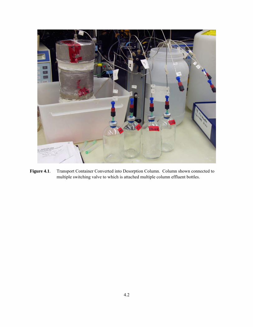
A column desorption experiment consisted of injecting groundwater from a well in Hanford’s 100 Area (i.e., free of CCl4 and CHCl3) into the solute-laden sediment core at a constant flow rate for up to a maximum of 20 pore volumes and collecting effluent samples for solute (CCl4, CHCl3) analysis (Figure 4.1). The column system was built specifically to minimize mass loss of the volatile solutes during the desorption experiment. A 5-liter bottle containing oxygen-saturated Hanford groundwater was connected to an Hitachi L-6200 HPLC pump, which supplied a constant flow rate (0.42 to 0.54 milliliters per minute, depending on experiment) through stainless steel tubing to the column inlet (total volume 1,010 cm3). The column effluent (flow vertically up in Figure 4.1) was plumbed to a flow-through electrical conductivity (EC) electrode (20-microliter volume), then to a Kloehn syringe pump with eight-channel multiplexing head. The EC electrode was connected to an EC meter and data logging system and used to monitor the conservative tracer. EC data was collected at a rate of 2 points per second and averaged for 1 minute. The conservative tracer breakthrough consisted of the small change in electrical conductivity between the groundwater in the sediment column and influent water. The Kloehn syringe pump was connected to seven 154 milliliter septa-top glass bottles and a large waste bottle. The syringe pump was used as a fraction collector, where column effluent flowed into a septa-top bottle for 74 minutes (30 milliliters), then into the waste bottle for a specified time (0 to 40 hours). Sample collection frequency was designed to collect more samples during initial breakthrough (<2 pv), and less samples along the “tail” of the break through curve (2 to 20 pv). Between 0 and 1.75 pore volumes, the sample collection frequency was one per 75 minutes. From 1.75 to 5 pore volumes the sample collection frequency was one per 300 minutes. From 5 to 20 pore volumes, the sample collection frequency was one per 40 hours, giving a total experiment time of 200 to 220 hours.

The 30 milliliters of aqueous effluent in the sealed septa-top vials were expected to achieve liquid-gas phase equilibrium within 40 to 96 hours before GC-MS analysis of the solutes in the vapor phase. Henry’s Law (at 25ºC [77ºF]) was used to calculate the total solute mass originally in the liquid given the gas phase measurement, as described in Appendix A. A total of four column experiments were conducted (named T15, T17, T18, and T19), with effluent data profiles of electrical conductivity (i.e., nonreactive tracer) and CCl4 and/or CHCl3 concentration with time (Appendix B). Column porosity was calculated from values of sediment wet weight and dry weight for each column experiment. The dry bulk density was calculated from sediment dry weight and total column volume for each experiment. The flow rate for all column experiments was chosen to be 10 to 5 hours per pore volume, which was considered sufficient time for solutes to desorb from the sediment or organic matter surfaces (assuming no extremely slow physical or chemical kinetic processes are occurring) and produce desorption profiles for simulation modeling and determination of CCl4 and CHCl3 partition coefficients.

After completion of an experiment, the column was dismantled, and subsamples of the sediment core were analyzed for solutes according to procedures described in Sections 3.4 and 3.5.

4.2

Figure 4.1. Transport Container Converted into Desorption Column. Column shown connected to multiple switching valve to which is attached multiple column effluent bottles.

5.1

5.0 Tracer/Solute Profile Simulations from 1-D ColumnExperiments

5.1 Partition Coefficients from Profile Determination of RetardationFactors

The “retardation factor” (Rf) is defined by the ratio of velocities of the tracer/solute so that avalue of 1.0 indicates no sorption (solute travels at the same velocity as the tracer) and a value >1.0indicates sorption. With no additional assumption as to the sorption mechanism or rate, the soluteretardation factor was determined by integrating the area in front of the solute breakthrough curve.The sorption mass parameter Kd (cm3/g or L/Kg) is defined by the mass of solute on the sedimentsurface (per gram of sediment) to the mass of solute in aqueous solution (per milliliters of solution),and can be calculated from Rf by:

Rf = 1 + rbKd/q (5.1)

where rb is the dry bulk density (g/cm3) and q is the total porosity. Reactive transport simulations ofbreakthrough was additionally done to validate different conceptual models that describe solutesorption/desorption (described in the following section).

5.2 Model Simulations to Assess Tracer/Solute Behavior

Three different reactive transport models were used to quantify kinetic parameters that describesolute slow sorption/desorption and diffusion of tracer and solute between mobile and immobile porefluid pore fluid. These models were:

• equilibrium model – incorporates advective/dispersive flux and rapid (equilibrium) sorption

• first-order model – incorporates advective/dispersive flux and first-order reversible slow(kinetic) sorption/desorption

• two-region model – incorporates advective/dispersive flux, equilibrium and first-orderkinetic sorption or diffusion between mobile and immobile pore fluidand equilibrium sorption in both regions.

A systematic approach was used to determine model parameters independently of fitting multipleparameters to a single breakthrough curve because both hydrodynamic dispersion and slow sorption/desorption will define the solute breakthrough curve shape. This required using the Kd valuesdetermined from area integration (described above) and using longitudinal dispersivity (DL) valuesfrom fitting tracer breakthrough data. Longitudinal dispersivity (DL) is defined by the physicalbreakthrough curve spreading that occurs as a nonsorbing (conservative) tracer flows through a 1-Dporous media column:

DL = Do + aL v (5.2)

where Do is molecular diffusion, aL is the longitudinal dispersivity, and v is the interstitial velocity.Idealized transport of a sorbing solute in the same homogeneous sediment column will have the same

5.2

longitudinal dispersion (producing breakthough curve spreading) but will lag relative to the tracer dueto the reversible sorption/desorption (i.e., Rf). A pore volume is defined by the volume of water inthe sediment column that is subjected to advective/dispersive transport. The reactive transportmodel that describes rapid (equilibrium) sorption, advection, and dispersion is described by thedifferential equation:

Rf rbq

∂S∂t = DL ∂

2C∂z2 - v ∂C

∂z (5.3)

The model includes three parameters; velocity (v), retardation factor, (Rf), and longitudinaldispersion (DL) to describe the rate of change in the solute or tracer aqueous concentration (C) orsurface concentration (S), as first described by Gleuckauf (1947). An analytical solution to thismodel with a nonlinear least squares parameter estimation routine was first described by vanGenuchten and others (1974, 1979), and used here in it’s current form (CXTFIT, Toride et al. 1993,1999). In this study the tracer data was fit with the equilibrium model to determine the longitudinaldispersion, with a defined velocity and defined retardation factor (1.0; i.e., the velocity andretardation factor were not allowed to vary in the simulation, only the dispersion). Next, the solutedata was fit with this equilibrium model with the velocity fixed and longitudinal dispersion fixed at thetracer value (i.e., allowing Rf to vary). If the solute data could be well fit with this equilibrium modelsimulation, then there was no additional breakthrough curve spreading caused by slowsorption/desorption of the solute. Additional breakthrough curve spreading (greater than that definedby longitudinal dispersion) indicated slow chemical/physical release of the solute from the surface,and required the use of the first-order or two-region model to approximate the additional kineticprocess(es).

The first-order model describes advective-dispersive transport with reversible, linear adsorption/desorption reaction is defined by the solution to the differential equations

∂C∂t + rb

q ∂S∂t = D ∂

2C∂z2 - v ∂C

∂z (5.4)

rbq

∂S∂t = kf C - kb S

(5.5)

with previously defined parameters. This first-order kinetic model contains four parameters;velocity, longitudinal dispersion, and the two reaction rate parameters (kf, kb), which are defined by afirst-order reversible reaction:

(5.6)

5.3

accounts for reversible slow adsorption and slow desorption where kf is the forward rate coefficientand kb is the backward rate coefficient. Note that Kd = S/C = kf/kb. The first-order kinetic model wasfirst fit to 1-D solute transport data in sediments by Leenheer and Ahlrichs (1971). The first-ordermodel was used in this study with the longitudinal dispersivity fixed, and allowing both retardationfactor and kb (desorption rate coefficient) to vary to determine if this simple reaction couldrepresent the observed data.

The two-region model describes solute advective/dispersive transport through a porous mediawith both mobile (subscript “e”) and immobile (subscript “i”) pore regions and equilibrium sorption inboth regions (van Genuchten et al. 1974), as defined by the differential Equations (5.7) and (5.8)

qe∂Ce∂t + qi

∂Ci∂t + f rb ∂Se

∂t + (1 - f) rb ∂Si∂t = DL ∂

2Ce∂z2 - vqe

∂C∂z (5.7)

qi∂Ci∂t + (1 - f) rb ∂Si

∂t = ae (Ce - Ci)(5.8)

where f is the fraction of sorbent in the mobile region, Ce and Ci are solute concentrations in themobile and immobile regions, respectively; Se and Si are the respective sorbed concentrations, and qe

and qi are the volume fractions of the mobile and immobile liquid regions. This two-region model hasfive parameters: velocity (v), longitudinal dispersion (DL), equilibrium sorption (Kd = S/C),diffusional mass transfer between mobile and immobile pore fluid (ae), and the fraction solute mass inthe mobile region (f). The two-region model is mathematically equivalent to a fast and slow reactionin parallel or in series. In this study, the two-region model was fit to T17 tracer data because a poorfit of the equilibrium and first-order model indicated the presence of mobile-immobile pore fluidregions (i.e., heterogeneities). The two-region model was fit to T17 solute data fixing thelongitudinal dispersivity and fraction of mobile pore fluid (f) at the tracer values.

The code CXTFIT contains analytical solutions to the equilibrium model (i.e., Equation [5.3]),the first-order model (Equations [5.4] and [5.5]), and the two-region model (Equations [5.7] and[5.8]). How well simulations of solute breakthrough with the equilibrium, first-order, and two-regionmodels fit breakthrough data indicated whether the conceptual model was valid. In general a poormodel fit indicated that the mathematical description of the physical and chemical processes wasinsufficient to describe the actual data. Progressively more complex models were used if simulationscould not describe the breakthrough data, as indicated by the following scenarios:

(i) equilibrium model shows a good fit to both tracer and solute breakthrough data. This indicatesan equilibrium sorption reaction (Kd = S/C) was likely occurring.

(ii) equilibrium model fit to tracer data, but solute data has a poor fit with the equilibrium modeland a good fit with the first-order model. This indicates equilibrium sorption of the solute was notoccurring, and a reversible first-order kinetic model could represent the sorption/desorption rateoccurring.

5.4

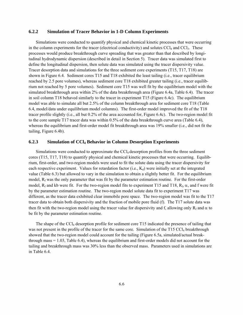
(iii) equilibrium model fit to tracer data, but solute data has a poor fit with the equilibrium andfirst-order model and a good fit with the two-region model. This indicates equilibrium sorption andfirst-order reversible kinetic sorption was not occurring, but a more complex process(es) wasoccurring.

6.1

6.0 Results

6.1 Physical and Chemical Characteristics of Sediment Cores

Table 6.1 summarizes the bulk fraction distribution of four sediment core samples taken adjacent to sediment cores (i.e., within 6 inches) used in the desorption experiments. Bulk fraction distributions in these cores were assumed to be the same as those used in the desorption experiments as visual examina-tion of these cores’ bulk fraction features showed no observable differences from those of the cores used in the desorption experiments. Core samples A and B, representing desorption experiments T15 and T17, had similar distributions with approximately 87 to 92% of the mass associated with the gravel and sand fractions. This is in contrast to core sample C, representing desorption experiment T18, which contained a high sand content (83.5%) and virtually no gravel. Among these three samples, sample C had the largest combined silt/clay content. Core sample D, representing desorption experiment T19, had a combined silt/clay content of 82.2% (36.7% clay).

The organic carbon content of all four cores was low (<0.1%) (Table 6.2). Core D contained the highest organic carbon content (0.088%), while core samples A and C contained the lowest (0.024% and 0.017%, respectively). Core sample B contained the highest inorganic carbon content (0.374%) possibly due to the presence of small amounts of calcium carbonate. Inorganic carbon was not detected in core samples A and C.

Table 6.1. Bulk Fraction (%) Classification of Aquifer Samples

Compositional Component A(a) (T15) B(b) (T17) C(c) (T18) D(d) (T19)

Gravel 57.5 66.5 1.88 8.21 Sand 29.0 25.6 83.5 9.53 Silt 10.2 6.02 10.2 45.5 Clay 3.39 1.97 4.42 36.7

(a) 230 to 232 feet. (b) 292 to 294 feet. (c) 364 to 366 feet. (d) 430 to 432 feet.

Table 6.2. Carbon Analysis of Aquifer Core Samples

Experiment Total Carbon (%) Inorganic Carbon (%) Organic Carbon (% by Difference) A (T15) 0.024 0.000 0.024 B (T17) 0.433 0.374 0.059 C (T18) 0.017 0.00 0.017 D (T19) 0.123 0.036 0.088

6.2

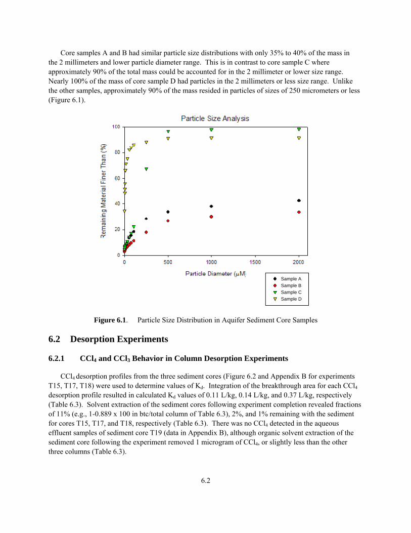
Core samples A and B had similar particle size distributions with only 35% to 40% of the mass in the 2 millimeters and lower particle diameter range. This is in contrast to core sample C where approximately 90% of the total mass could be accounted for in the 2 millimeter or lower size range. Nearly 100% of the mass of core sample D had particles in the 2 millimeters or less size range. Unlike the other samples, approximately 90% of the mass resided in particles of sizes of 250 micrometers or less (Figure 6.1).

Figure 6.1. Particle Size Distribution in Aquifer Sediment Core Samples

6.2 Desorption Experiments

6.2.1 CCl4 and CCl3 Behavior in Column Desorption Experiments

CCl4 desorption profiles from the three sediment cores (Figure 6.2 and Appendix B for experiments T15, T17, T18) were used to determine values of Kd. Integration of the breakthrough area for each CCl4 desorption profile resulted in calculated Kd values of 0.11 L/kg, 0.14 L/kg, and 0.37 L/kg, respectively (Table 6.3). Solvent extraction of the sediment cores following experiment completion revealed fractions of 11% (e.g., 1-0.889 x 100 in btc/total column of Table 6.3), 2%, and 1% remaining with the sediment for cores T15, T17, and T18, respectively (Table 6.3). There was no CCl4 detected in the aqueous effluent samples of sediment core T19 (data in Appendix B), although organic solvent extraction of the sediment core following the experiment removed 1 microgram of CCl4, or slightly less than the other three columns (Table 6.3).

Sample A Sample B Sample C Sample D

6.3

0

0.2

0.4

0.6

0.8

1

0 1 2 3 4 5

ECnormdata

pore vol

a)no

rmal

ized

con

c.

EC dataCCl4 data

0

0.2

0.4

0.6

0.8

1

0 2 4 6 8 10

ECnormF

pore vol

b)

norm

aliz

ed c

onc.

EC dataCCl4 data

0

0.2

0.4

0.6

0.8

1

0 2 4 6 8 10

ECnormdata

pore vol

c)

norm

aliz

ed c

onc.

EC dataCCl4 data

Figure 6.2. Tracer and Carbon Tetrachloride Breakthrough Data for Column Experiments T15 (a), T17

(b), and T18 (c)

6.4

CHCl3 desorption profiles from sediment cores T17 and T18 (Figure 6.3 and Appendix B) with a 20 pore volume water injection were used to calculate Kd values. Integration of the chloroform (CHCl3) breakthrough areas resulted in calculated Kd values of 0.43 L/kg and 0.084 L/kg for sediment cores T17 and T18, respectively (Table 6.3). No chloroform was detected in the effluent of sediment core T19 when subjected to aqueous desorption (detection limit 0.5 ppb). CHCl3 was not analyzed for in sediment core T15. Therefore, neither a desorption profile nor a value of Kd was generated for this sample. Solvent extraction of the sediment cores following experiment completion revealed fractions of 70%, and 61% remaining with the sediment for cores T17 and T18, respectively (Table 6.3).

0

0.2

0.4

0.6

0.8

1

0 2 4 6 8 10

ECnormB

pore vol

a)

norm

aliz

ed c

onc.

EC dataCCl3 data

0

0.2

0.4

0.6

0.8

1

0 2 4 6 8 10

ECnormB

pore vol

b)

norm

aliz

ed c

onc.

EC dataCCl3 data

Figure 6.3. Tracer and Chloroform Breakthrough Data for Column Experiments T17 (a) and T18 (b)

6.5

Table 6.3. Column Experiment Solute Mass Retardation and Mass Balance

6.6

6.2.2 Simulation of Tracer Behavior in 1-D Column Experiments

Simulations were conducted to quantify physical and chemical kinetic processes that were occurring in the column experiments for the tracer (electrical conductivity) and solutes CCl4 and CCl3. These processes would produce breakthrough curve spreading that was greater than that described by longi-tudinal hydrodynamic dispersion (described in detail in Section 5). Tracer data was simulated first to define the longitudinal dispersion, then solute data was simulated using the tracer dispersivity value. Tracer desorption data and simulations for the three sediment core experiments (T15, T17, T18) are shown in Figure 6.4. Sediment cores T15 and T18 exhibited the least tailing (i.e., tracer equilibrium reached by 2.5 pore volumes), whereas sediment core T18 exhibited greater tailing (i.e., tracer equilib-rium not reached by 5 pore volumes). Sediment core T15 was well fit by the equilibrium model with the simulated breakthrough area within 2% of the data breakthrough area (Figure 6.4a, Table 6.4). The tracer in soil column T18 behaved similarly to the tracer in experiment T15 (Figure 6.4c). The equilibrium model was able to simulate all but 2.5% of the column breakthrough area for sediment core T18 (Table 6.4, model/data under equilibrium model columns). The first-order model improved the fit of the T18 tracer profile slightly (i.e., all but 0.2% of the area accounted for, Figure 6.4c). The two-region model fit to the core sample T17 tracer data was within 0.5% of the data breakthrough curve area (Table 6.4), whereas the equilibrium and first-order model fit breakthrough area was 19% smaller (i.e., did not fit the tailing, Figure 6.4b).

6.2.3 Simulation of CCl4 Behavior in Column Desorption Experiments

Simulations were conducted to approximate the CCl4 desorption profiles from the three sediment cores (T15, T17, T18) to quantify physical and chemical kinetic processes that were occurring. Equilib-rium, first-order, and two-region models were used to fit the solute data using the tracer dispersivity for each respective experiment. Values for retardation factor (i.e., Kd) were initially set at the integrated value (Table 6.3) but allowed to vary in the simulation to obtain a slightly better fit. For the equilibrium model, Rf was the only parameter that was fit by the parameter estimation routine. For the first-order model, Rf and kb were fit. For the two-region model fits to experiment T15 and T18, Rf, α, and f were fit by the parameter estimation routine. The two-region model solute data fit to experiment T17 was different, as the tracer data exhibited clear immobile pore space. The two-region model was fit to the T17 tracer data to obtain both dispersivity and the fraction of mobile pore fluid (f). The T17 solute data was then fit with the two-region model using the tracer value for dispersivity and f, allowing only Rf and α to be fit by the parameter estimation routine.

The shape of the CCl4 desorption profile for sediment core T15 indicated the presence of tailing that was not present in the profile of the tracer for the same core. Simulation of the T15 CCl4 breakthrough showed that the two-region model could account for the tailing (Figure 6.5a, simulated/actual break-through mass = 1.03, Table 6.4), whereas the equilibrium and first-order models did not account for the tailing and breakthrough mass was 30% less than the observed mass. Parameters used in simulations are in Table 6.4.

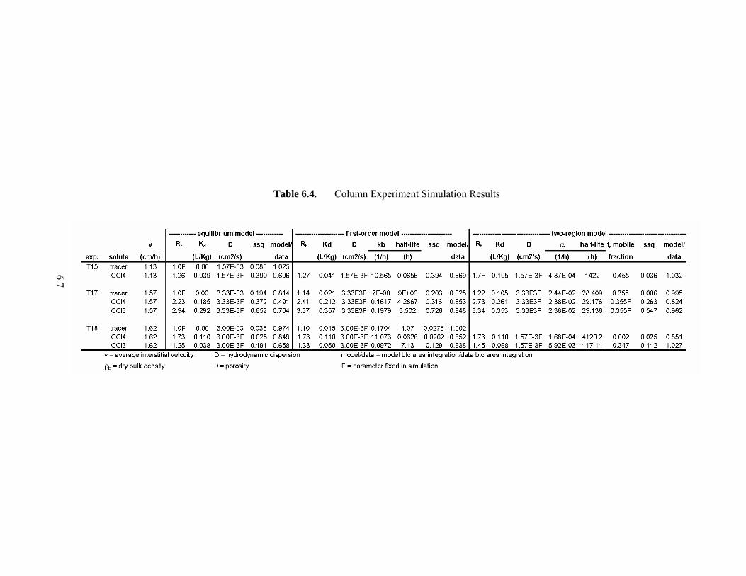
6.7

Table 6.4. Column Experiment Simulation Results

6.8

0

0.2

0.4

0.6

0.8

1

0 1 2 3 4 5

ECnormAEC

/EC

o

pore vol

a)

13.45 h/pvRf(EC) = 1.0001

EC dataeq model

T15 EC

0

0.2

0.4

0.6

0.8

1

0 1 2 3 4 5

ECnormeq mfo mtrEC

/EC

o

pore vol

b)

9.95 h/pvRf(EC) = 1.020

EC dataeq modelfirst order modeltwo region model

T17EC

0

0.2

0.4

0.6

0.8

1

0 1 2 3 4 5

ECnormeqfoEC

/EC

o

pore vol

c)

9.96 h/pvRf(EC) = 1.011

dataeq modelfirst order model

T18EC

Figure 6.4. Conservative Tracer Breakthrough Data for Column Experiments T15 (a), T17 (b), and T18 (c)

6.9

0

0.2

0.4

0.6

0.8

1

0 1 2 3 4 5

dataeq modfirst mtwo r mod

pore vol

a)no

rmal

ized

con

c.

T15CCl4

dataeq modelfirst order modeltwo region model

0

0.2

0.4

0.6

0.8

1

0 2 4 6 8 10

FBCD

pore vol

b)

norm

aliz

ed c

onc.

dataeq modelfirst order modeltwo region model

T17CCl4

0

0.2

0.4

0.6

0.8

1

0 2 4 6 8 10

dataeqfotr

pore vol

c)

norm

aliz

ed c

onc.

dataeq modelfirst order modeltwo region model

T18CCl4

Figure 6.5. Carbon Tetrachloride Breakthrough Data for Column Experiments T15 (a), T17 (b), and T18 (c)

6.10

The CCl4 desorption profile for sediment core T17 showed increased tailing relative to the tracer from the same core. CCl4 tailing extended the entire 17 pore volumes, as compared with tailing to 2.5 pore volumes for the tracer. Simulation of the T17 CCl4 breakthrough showed that the equilibrium model could only account for 49% of the breakthrough curve area, the first-order model only 65%, and the two region model 82%. The two-region model fit the general shape of the desorption profile (Figure 6.5b). Core T17 contained the highest inorganic and organic carbon content of the three cores, suggesting that the increased tailing (CCl4 resistance to desorption) may be related to these factor differences.

Simulation of CCl4 breakthrough for sediment core T18 was well fit by the equilibrium model, and the first-order and/or two-region models had the same fit.

6.2.4 Simulation of Chloroform Behavior in Column Desorption Experiments

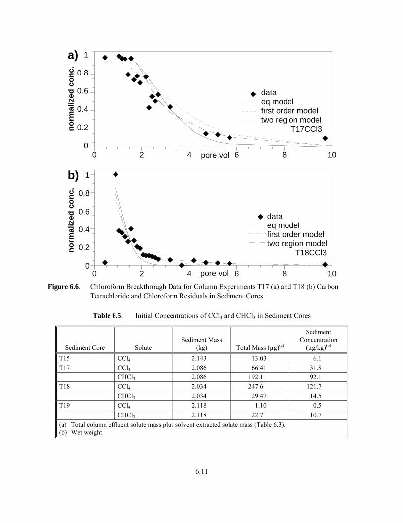
The shape of the CHCl3 desorption profiles for sediment cores T17 and T18 (Figure 6.6) exhibited similar tailing behavior, relative to the corresponding tracer profile as CCl4. Integration of the CHCl3 breakthrough areas resulted in calculated Kd values of 0.43 L/kg and 0.084 L/kg for sediment cores T17 and T18, respectively. The equilibrium model provided poor fits for the T17 and T18 sediment core CHCl3 profiles (i.e., 70% and 66% of the areas accommodated, respectively, Table 6.4). Fit improved when the first-order model was used, however, the two-region model was needed to effectively describe both profiles. The two-region model was able to accommodate all but 4% and 3% of the areas of the breakthrough data for sediment cores T17 and T18, respectively. Parameters used in simulations are in Table 6.4.

6.3 Carbon Tetrachloride and Chloroform Residuals in Sediment Cores

Solvent extraction of each of the four sediment cores was performed following aqueous desorption, and the distribution of mass between desorption effluent and sediment was determined (Table 6.4). The mass associated with the sediment includes the small amount of solute in water in contact with the sediment following desorption. Greater than 89% of the CCl4 was found to be associated with the column effluent for sediment cores T15, T17, and T18. While low, all the CCl4 mass in sediment core T19 was associated with the sediment. In contrast, a significant portion of CHCl3 was found to be associated with the sediment. Residual CHCl3 mass associated with sediment core T17 was 70%. For sediment core T18, residual mass was 61%.

6.4 Initial Sediment Core Solute Concentrations

Initial concentrations of CCl4 and CHCl3 in experimental sediment cores were determined from sediment core masses and solvent extracted solute mass. These results are summarized in Table 6.5. Observed concentrations of CCl4 ranged from 0.5 to 121.7 µg/kg while CHCl3 concentrations ranged from 10.7 to 92.1 µg/kg. Very little, if any, CCl4 was determined to be present on the sediment of core T19.

6.11

0

0.2

0.4

0.6

0.8

1

0 2 4 6 8 10

Beqfotr

pore vol

a)no

rmal

ized

con

c.

T17CCl3

dataeq modelfirst order modeltwo region model

0

0.2

0.4

0.6

0.8

1

0 2 4 6 8 10

BEFG

pore vol

b)

norm

aliz

ed c

onc.

dataeq modelfirst order modeltwo region model

T18CCl3

Figure 6.6. Chloroform Breakthrough Data for Column Experiments T17 (a) and T18 (b) Carbon

Tetrachloride and Chloroform Residuals in Sediment Cores

Table 6.5. Initial Concentrations of CCl4 and CHCl3 in Sediment Cores

Sediment Core Solute Sediment Mass

(kg) Total Mass (µg)(a)

Sediment Concentration

(µg/kg)(b)

T15 CCl4 2.143 13.03 6.1 T17 CCl4 2.086 66.41 31.8 CHCl3 2.086 192.1 92.1 T18 CCl4 2.034 247.6 121.7 CHCl3 2.034 29.47 14.5 T19 CCl4 2.118 1.10 0.5 CHCl3 2.118 22.7 10.7 (a) Total column effluent solute mass plus solvent extracted solute mass (Table 6.3). (b) Wet weight.

6.12

6.5 Concentrations of Solutes in Samples of Groundwater Collected at Sediment Depth Locations

Table 6.6 summarizes the results of analysis of groundwater samples from well 299-W15-46 at those depths where sediment samples were collected for column desorption. The table includes results obtained from the Fluor Hanford, Inc. field laboratory and PNNL’s fixed analytical laboratory. Good agreement was observed on the results from separate samples collected from the same depth. CCl4 concentrations ranged from 825 to 2,463 ppb at an aquifer depth ranging from 71.6 to 111 meters (235 to 365 feet). Chloroform concentrations ranged from 37 to 400 ppb over the same depth range. Trichloroethene was detected at concentration levels in the 2 to 10 ppb range. The highest concentration, for all three compounds was observed at a depth of 89 to 89.6 meters (292 to 294 feet). We were unable to obtain a representative groundwater sample from a depth of 70 to 70.7 meters (230 to 232 feet) for analysis. For the purpose of the column desorption experiment on the sediment core from 70 to 70.7 meters (230 to 232 feet), it was assumed that the solute concentrations in the groundwater at 71.6 meters (235 feet) was the same as at a depth of 70 to 70.7 meters (230 to 232 feet). A groundwater sample could not be obtained from a depth of 131 to 131.7 meters (430 to 432 feet) because of the nature of the formation (i.e., Lower Ringold Mud-confining layer that separates the unconfined aquifer from the upper confined aquifer at this location).

Table 6.6. Summary of Groundwater Solute Data. Solute Concentration in µg/L

Groundwater Depth meters(feet) Carbon Tetrachloride Chloroform Trichloroethene

70-70.7 (230-232) ND(a) ND(a) ND(a)

71.6 (235)(b) 2,239 37 6.7 81.7 (268)(c) 825 43 10

89-89.6 (292-294)(d) 2,463 ± 50 (n=3) 400 ± 10 (n=3) 8 ± 0.4 (n=3) 111-111.6 (364-366)(e) 1,145 ± 20 (n=3) 123 ± 5 (n=3) 2 ± 2 (n=3) 131-131.7 (430-432) ND(f) ND(f) ND(f)

(a) Method of groundwater collection at this depth (bailer) precluded collection of suitable groundwater samples. (b) Results from Fluor Hanford, Inc. field laboratory analysis. (c) Results from Fluor Hanford, Inc. field laboratory analysis. PNNL analysis of groundwater from same depth measured a CCl4 concentration of 795 µg/L. (d) Fluor Hanford, Inc. field laboratory analysis results were 2,918 µg/L (carbon tetrachloride), 413 µg/L (chloroform), and 11.0 µg/L (trichloroethene). (e) Fluor Hanford, Inc. field laboratory analysis results were 1,174 µg/L (carbon tetrachloride), 152 µg/L (chloroform), and 7.2 µg/L (trichloroethene). (f) No data.

6.6 Predicted Versus Observed Kd Values

Partition coefficient values from this study (Table 6.3) were compared to those predicted from equations that calculate values of Kd based on sediment organic fraction (foc) and estimates of the normalized sorption coefficient (Koc) (Truex et al. 2001) (Table 6.7). Observed CCl4 Kd values (this

6.13

Table 6.7. Predicted Versus Observed Kd Values

Core Solute Kd

(observed)(a) OC

(%)(b) foc

Koc (eq3)(c) Kd (eq3)

Kd(obser)/ Kd (Cal)

Koc (eq4)(c) Kd (eq4)

Kd(obser)/ Kd (Cal)

T-15 CCl4 0.106 0.024 0.00024 110.48 0.0265 4 161.11 0.0387 2.7 T-17 CCl4 0.367 0.059 0.00059 110.48 0.0651 5.6 161.11 0.0951 3.9 CHCl3 0.432 0.059 0.00059 30.72 0.0181 23.9 38.26 0.0226 19.1 T-18 CCl4 0.144 0.017 0.00017 110.48 0.0188 7.6 161.11 0.0274 5.3 CHCl3 0.084 0.017 0.00017 30.72 0.0052 16.8 38.26 0.0065 12 (a) From Table 6.3, this study. (b) From Table 6.2. (c) From Table 1 of Truex et al. 2001. Equation 3: log (Koc) = 3.64 – 0.55 X log (S) where S is the water solubility of the solute (mg/L). Equation 4: log (Koc) = 4.277 – 0.557 X log (Sm) where Sm ios the molar water solubility of the solute (µmol/L).

study) were 3 to 8 times higher than predicted depending on which of the two equations were applied. Observed CHCl3 Kd values (this study) were 12 to 24 times higher than predicted depending on which of the two equations were applied.

6.7 Predicted Versus Observed Sediment Core Solute Concentrations Groundwater concentrations of CCl4 and CHCl3 (Table 6.6) and the corresponding experimentally determined partition coefficients for three of the sediment core experiments (Table 6.3) were used to predict solute concentrations in the corresponding sediments assuming equilibrium existed between groundwater and sediment. These concentrations were compared to the initial solute concentrations observed to be present in the sediment cores. The results are summarized in Table 6.8. Predicted concentrations of CCl4 were significantly higher than observed in the three sediment cores, particularly sediment cores T15 and T17. In these two cores, observed concentrations were 2.8% and 3.5% of predicted values, respectively. The observed concentration of CCl4 in sediment core T18 was 73.8% of the predicted value. The observed CHCl3 concentration in soil core T17 was 53.2% of that predicted whereas the predicted CHCl3 concentration was closer to the concentration observed in sediment core T18. Since Kd values were not determined for sediment core T19, a comparison could not be made for that sample.

Table 6.8. Predicted Versus Observed Sediment Solute Concentrations

Experiment Compound Kd (L/kg)

Groundwater Concentration

(µg/L)

Predicted Sediment

Concentration (µg/kg)

Observed Sediment

Concentration (µg/kg)

T15 CCl4 0.106 2,239 237 6.1

T17 CCl4 0.367 2,463 904 31.8

CHCl3 0.432 400 173 92.1

T18 CCl4 0.144 1,145 165 121.7

CHCl3 0.084 123 10 14.5

T19 CCl4 0.5

CHCl3 10.7

7.1

7.0 Discussion

Intact sediment cores were collected from borehole 299-W15-46 located adjacent to the 216-Z-9 trench at the Hanford Site’s 200 West Area. Four split spoon samples were collected at unconfined aquifer depths of 70 to 70.7 meters (230 to 232 feet), 89 to 89.6 meters (292 to 294 feet), 111 to 111.6 meters (364 to 366 feet) and 131 to 131.7 meters (430 to 432 feet), respectively. The borehole was drilled into the CCl4 plume at a location where groundwater concentration of CCl4 concentration was anticipated to be in the range of 1 to 2 parts per million. Therefore, it was also anticipated that the collected aquifer sediments would be contaminated with CCl4, CCl4 degradation products and perhaps other solute compounds. Solute contaminants identified would have been in contact with these sediments for at least 30 years when discharges to the trench had ceased (DOE 2001). The nature of these sediments afforded an opportunity to perform aqueous desorption experiments to assess the effects of long contact time on organic solute transport in aquifer sediments. Such experiments are not easily simulated in the laboratory where contact times are limited as a result of concern over the ability to control degradation processes. Sediment cores from each of the disassembled split spoon samplers were brought back to the laboratory. Aqueous desorption experiments were performed on these samples within a few days of their arrival at the laboratory to ensure sample quality and stability.

Chemical analysis of sediment cores from each depth showed the presence of the organic solutes CCl4, CHCl3, methylene chloride, and trichloroethene. Chemical analysis of column effluent samples for methylene chloride was confounded by suspect sample contamination. Concentrations of trichloroethene in column effluent were near the analytical limit. Therefore, desorption profile data collection was limited to CCl4 and CHCl3.

Area integration of tracer/solute curves (profiles) was used to calculate partition coefficients, taking into account any dispersivity effects identified from the conductivity profiles. CCl4 Kd values were in the range 0.106 to 0.367 L/kg, in which the sediment organic carbon contents were less than 0.1% (0.017 to 0.059%). For the two sediments where CHCl3 was measured, CHCl3 Kd values were 0.432 L/kg and 0.084 L/kg, respectively. Previously, Truex et al. (2001) estimated the Kd (based on Koc) for CCl4 in a Hanford soil with an averaged organic carbon content of 0.2%. The Kd was estimated to be in the range of 0.016 to 0.83 L/kg with a most probable value in this range of 0.12 L/kg (Truex et al. 2001); on the low end of the range of values calculated in this study. The best estimate value of Truex et al. 2001 would be 0.06 L/kg based on a 0.1% sediment organic carbon content.

At levels of organic carbon above 0.1%, Koc can be used to estimate the Kd of an organic compound if the organic carbon content of the sediment is known. Past research suggests that application of this relationship to sediments with organic carbon content below 0.1% (e.g., at Hanford) may under-predict sorption in sediment. For example, a CCl4 Kd value of 0.39 ml/g was reported for a soil with an organic carbon content of less than 0.03% (Zhao et al. 1999). In contrast, the predicted Kd (based on Koc) for CCl4 in a soil with an organic carbon content of 0.03% was shown to range from 0.015 to 0.081 ml/g (Truex et al. 2001). Values of CCl4 and CHCl3 partition coefficients from this study support these earlier observations, where CCl4 and CHCl3 Kd’s from this study were 3-8 and 12-23 times larger than would be

7.2

predicted based on sediment organic carbon content, so may be sorbing to mineral surfaces such as clays and iron oxides.

The significant differences between observed versus predicted (i.e., lower) concentrations of CCl4 in sediment cores (e.g., T15 and T17; Table 6.8) suggest the occurrence of CCl4 degradation in these sediments. CHCl3 can be produced by abiotic dechlorination of CCl4 by a reductant such as adsorbed ferrous iron on an iron oxide on 2:1 smectite clay (Amonette et al. 2000). CCl4 appeared to show little affinity for sediment as demonstrated by most of the CCl4 in the desorption experiments to be associated with the aqueous effluent streams (i.e., 89 to 99%). Evidence for the presence of contaminant resistant fractions in soils and sediments for a wide range of organic contaminants has been summarized in past reviews (Pignatello and Xing 1996; Luthy et al. 1997). A significant amount of CHCl3 from sediment cores T17 (70% of the total mass) and T18 (61% of the total mass) resisted desorption, indicating its presence as a resistant fraction. Sediment cores T17 and T18 contained small clay fractions (2 to 4%, respectively). One possibility is that CHCl3 has been absorbed into elements of the mineral fraction of the sediments (e.g., the interlayer components of clays) over many years of interaction following abiotic formation from CCl4. This would be consistent with the resistive behavior of CHCl3 observed in these sediment cores and the similar behavior observed in the high clay content core from the Ringold Formation (T19). The difference in sediment sorption behavior of CCl4 versus CHCl3 may relate to the difference in their structure and the type of interaction that may occur with sediment (i.e., van der waals vs. hydrogen bonding).

The ease of extraction of residual CHCl3 with methanol suggests that CHCl3 is not permanently sequestered, and its release from sediment into migrating groundwater is controlled by multiple kinetic processes (e.g., diffusion out of meso- and micropores of sediment grains or from between clay layers, or out of organic matter coated on sediment grains). The degradation and sequestering properties of these sediments suggests that a certain portion of the CHCl3 in Hanford aquifer sediments is migrating quite slowly in groundwater. Also, the physical characteristics of the Ringold Formation mud unit (e.g., high silt and clay content) suggests that this unit is a good barrier to preventing CCl4 contamination of the upper confined aquifer.

The relatively few column experiments in this study showed a range of transport behavior that indicated the presence of both physical and chemical kinetic processes were at least partially controlling the release of solutes from the sediments. Tracer transport in two column experiments (T15, T18) exhibited equilibrium transport, but tracer transport in one column (T17) indicated the presence of mobile and immobile pore fluid. Simulation of the tracer breakthrough curve required the use of a two-region model, which describes diffusion between mobile and immobile pore fluid. Although tracer transport in the two other experiments (T15 and T18) was equilibrium-like, both carbon tetrachloride and chloroform desorption curves exhibited significant tailing greater than was caused by dispersion. Because there was no physical kinetic process (i.e., immobile/mobile pore fluid) apparent from tracer breakthrough, the slow release of these solutes from sediment surfaces was chemically controlled. Because simple organic compounds such as these should exhibit reversible partitioning to soil organic matter or mineral surfaces, this behavior could be indicative of an aging process resulting in stronger solute retention given the decades of contact time. Simulation of carbon tetrachloride and chloroform desorption was well approximated with a two-region kinetic model, and in some cases a first-order kinetic model, but were

7.3

poorly fit with an equilibrium model. Simulation fits with the two kinetic models is indicative of the presence of one or more kinetic processes partially controlling the release of solutes from the sediment.

Recent site-wide modeling of the transport of CCl4 in aquifer sediment assumed advective transport (Kd = 0 and no degradation) and a continuous groundwater source for several case simulations (Bergeron and Cole 2004). Results indicated exceedence of compliance limits outside the Central Plateau waste management area and at the Columbia River during a 1,000-year period of simulation. Application of a best estimate Kd value of 0.322 L/kg and CCl4 half-life of 0.00956 y-1 resulted in no exceedence of compliance limits at the same location after 1,000 years of simulation. From these results, the authors indicated how critical it is to have realistic values for these parameters for predicting the future movement of CCl4 from the 200 West Area. CCl4 and CHCl3 partition coefficients determined in this study are realistic in that they were obtained from Hanford sediments where CCl4 and CHCl3 had been in contact with the aquifer sediments for up to 30 years. The range in CCl4 partition coefficients in Hanford aquifer sediments from this study (0.106 L/kg to 0.367 L/kg) was lower by greater than a factor of ten as compared to the range estimated by Truex et al. (2001) of 0.016 L/kg to 0.83 L/kg based on Koc. Use of this studies Kd values in future simulations will result in more realistic predictions of CCl4 transport in Hanford groundwater with reduced uncertainty. The presence of significant concentrations of CHCl3 in the presence of lower-than-expected concentrations of CCl4 indicated CCl4 degradation in the sediment and the need to more accurately represent this process in transport modeling

8.1

8.0 References

American Society of Agronomy (ASA). 1986a. “Hydrometer Method.” Chapter 15-5 in Methods of Soil Analysis-Part 1, 2nd Edition of Physical and Mineralogical Methods, SSSA Book Series No. 5, ed. A Klute, pp. 404-408. Soil Science Society of America, Madison, Wisconsin.

American Society of Agronomy (ASA). 1986b. “Pynchnometer Method.” Chapter 14-3 In Methods of Soil Analysis-Part 1, 2nd Edition of Physical and Mineralogical Methods, SSSA Book Series No. 5, ed. A Klute, pp. 378-379. Soil Science Society of America, Madison, Wisconsin.

American Society for Testing and Materials (ASTM) D4129-88. 1988. “Standard Test Method for Total and Organic Carbon in Water by High Temperature Oxidation and by Coulometric Detection.” American Society for Testing and Materials, West Conshohocken, Pennsylvania.

American Society for Testing and Materials (ASTM) D2216-98. 1998. “Test Method for Laboratory Determination of Water (Moisture) Content of Soil and Rock.” American Society for Testing and Materials, West Conshohocken, Pennsylvania.

Amonette J, D Workman, D Kennedy, J Fruchter, and Y Gorby. 2000. “Dechlorination of Carbon Tetrachloride by Fe(II) Associated with Goethite.” Environmental Science and Technology 34(21):4606-4613.

Bauer RG and VJ Rohay. 2004. Data Quality Objectives Summary Report for Investigation of Dense, Non-Aqueous-Phase Liquid Carbon Tetrachloride in the 200 West Area. CP-15373, Rev. 0, Fluor Hanford, Richland, Washington.

Bergeron M.P and CR Cole. 2004. Recent Site-Wide Transport Modeling Related to the Carbon Tetrachloride Plume at the Hanford Site. PNNL-14855, Pacific Northwest National Laboratory, Richland, Washington.

DOE. 2001. Plutonium/Organic Rich Process Condensate/Process Waste Group Operable Unit RI/FS Work Plan: Includes the 200-PW-1, 200-PW-3, and 200-PW-6 Operable Units. DOE/RL-2001-01, Rev. 0, Re-Issue. U.S. Department of Energy, Richland, Washington.

EPA. 2000. Test Methods for Evaluating Solid Waste, Physical/Chemical Methods (SW-846), Chapter 4, Organic Analytes, Table 4-1. U.S. Environmental Protection Agency, Washington, D.C.

Gleuckauf E. 1947. “Theory of Chromatography, Part II-V.” J. Chemistry Society, 36, 1302-1329.

Hartman MJ, LF Morasch, and WD Webber. 2002. Hanford Site Groundwater Monitoring for Fiscal Year 2001. PNNL-13788, Pacific Northwest National Laboratory, Richland, Washington.

Leehneer J and J Ahlrichs. 1971. “A Kinetic and Equilibrium Study of the Adsorption of Carbaryl and Parathion Upon Soil Organic Matter.” Soil Science Society of America Proceedings, 35,700-05.

8.2

Luthy RG, GA Aiken, MI Brusseau, SD Cunningham, PM Gschwend, JJ Pignatello, M Reinhard, SJ Traina, WJ Weber, Jr, and JC Westall. 1997. “Sequestration of Hydrophobic Organic Contaminants by Geosorbents.” Environmental Science and Technology 31:3341-3347.

Pignatello, JJ and B Xing. 1996. “Mechanisms of Slow Sorption of Organic Chemicals to Natural Particles.” Environmental Science and Technology 30:1-11.

Serne RJ, BN Bjornstad, DG Horton, DC Lanigan, CW Lindenmeier, MJ Lindberg, RE Clayton, VL LeGore, KN Geiszler, SR Baum, MM Valenta, IV Kutnyakov, TS Vickerman, RD Orr, and CF Brown. 2004. Characterization of Vadose Zone Sediments Below the T Tank Farm: Boreholes C4104, C4105, 299-W10-196 and RCRA Borehole 299-W11-39. PNNL-14849, Pacific Northwest National Laboratory, Richland, Washington.

Toride N, FJ Leij, and MTh van Genuchten. 1993. “A Comprehensive Set of Analytical Solutions for Nonequilibrium Solute Transport with First-Order Decay and Zero-Order Production.” Water Resources Research, 29, 2167-2182, 1993.

Toride N, FJ Leij, and MTh van Genuchten. 1999. The CXTFIT Code for Estimating Transport Parameters from Laboratory or Field Tracer Experiments. Research report No. 137, Version 2.1, U.S. Salinity Laboratory, Agricultural Research Service, U.S. Department of Agriculture, Riverside, California.

Truex MJ, CJ Murray, CR Cole, RJ Cameron, MD Johnson, RS Skeen, and CD Johnson. 2001. Assessment of Carbon Tetrachloride Groundwater Transport in Support of the Hanford Carbon Tetrachloride Innovative Technology Demonstration Program. PNNL-13560, Pacific Northwest National Laboratory, Richland, Washington.

van Genuchten M. and R Cleary. 1979. “Movement of Solutes in Soil; Computer Simulated and Laboratory Results in Soil Chemistry.” In Physico-Chemical Models, pp 349-386, Elsevier Science, New York.

van Genuchten M, J Davidson, and P Wierenga. 1974. “An Evaluation of Kinetic and Equilibrium Equations for the Prediction of Pesticide Movement through Porous Media.” Soil Science Society of America Proceedings 38:29-35.

Zhao X, MJ Szafranski, MA Maraqa, and TC Voice. 1999. “Sorption of Carbon Tetrachloride in a Low Organic Carbon Content Sandy Soil.” Environ. Tox. and Chem. 18:1755-1762.

Appendix A

Calculation of Volatile Chlorinated Hydrocarbon Concentration from GC-MS Data

A.1

Appendix A

Calculation of Volatile Chlorinated Hydrocarbon Concentration from GC-MS Data

Aqueous effluent samples (30 milliliters) from one dimensional column experiments were collected and analyzed in a way that minimized volatilization and sorptive losses of volatile chlorinated hydro-carbon in the samples. The columns and associated tubing were all of stainless steel (as opposed to plastic) to minimize sorptive losses. Effluent samples were collected in 125 or 154 milliliters glass bottles with 1-cm thick septa to minimize CH loss due to volatilization through the use of all stainless steel columns and tubing in the column system to eliminate diffusion (through plastics). The gas chromatograph (GC) – mass spectrometer (MS) analysis was conducted on the gas headspace (Section 3.1), and the original mass of the CH in the aqueous phase was calculated as described in the following paragraphs.

The equilibrium partitioning of compounds between aqueous and gas phases can be quantified using Henry’s Law with dimensionless coefficients for carbon tetrachloride (CCl4 1.0756), chloroform (CHCl3 0.157), trichloroethene (TCE 0.372), and pentaflurobenzene (PFB 0.341). The fraction of solute mass in the gas phase (Fg) at equilibrium in a fixed volume container is calculated at 25ºC from:

Fg = 1/[1 + [Vaq/[KH – (Vtotal – Vaq)]]] (A.1)

where KH = the dimensionless Henry’s Law coefficient

Vtotal = the total volume of the vial (125 or 154 mL)

Vaq = the aqueous sample volume

The calculated fraction of solute mass in the gas phase (Figure A.1) shows that for very small volumes of water (i.e., <5 milliliters in the 154 milliliters vial), >98% of the organic mass is in the gas phase. With larger liquid volumes, the fraction in the gas phase is smaller. Carbon tetrachloride has the largest partition coefficient (i.e., is the most volatile), so a larger fraction remains in the gas phase relative to PFB, which is less volatile.

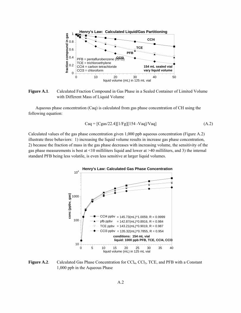
A.2

0

0.2

0.4

0.6

0.8

1

0 10 20 30 40 50

frac

tion

com

poun

d in

gas

liquid volume (mL) in 125 mL vial

Henry's Law: Calculated Liquid/Gas Partitioning

PFB

CCl4

154 mL sealed vialvary liquid volume

TCE

CCl3PFB = pentaflurobenzene (ISTD)TCE = trichloroethyleneCCl4 = carbon tetrachlorideCCl3 = chloroform

Figure A.1. Calculated Fraction Compound in Gas Phase in a Sealed Container of Limited Volume with Different Mass of Liquid Volume

Aqueous phase concentration (Caq) is calculated from gas phase concentration of CH using the following equation:

Caq = [Cgas/22.4][1/Fg][154 -Vaq]/Vaq] (A.2)

Calculated values of the gas phase concentration given 1,000 ppb aqueous concentration (Figure A.2) illustrate three behaviors: 1) increasing the liquid volume results in increase gas phase concentration, 2) because the fraction of mass in the gas phase decreases with increasing volume, the sensitivity of the gas phase measurements is best at <10 milliliters liquid and lower at >40 milliliters, and 3) the internal standard PFB being less volatile, is even less sensitive at larger liquid volumes.

10

100

1000

104

0 5 10 15 20 25 30 35 40

CCl4 ppbvpfb ppbvTCE ppbvCCl3 ppbv

conc

(ppb

v, g

as)

liquid volume (mL) in 125 mL vial

Henry's Law: Calculated Gas Phase Concentration

conditions: 154 mL vial liquid: 1000 ppb PFB, TCE, CCl4, CCl3

= 145.73(mL)^1.0059, R = 0.9999 = 142.87(mL)^0.8916, R = 0.984 = 143.21(mL)^0.9019, R = 0.987 = 135.32(mL)^0.7855, R = 0.954

Figure A.2. Calculated Gas Phase Concentration for CCl4, CCl3, TCE, and PFB with a Constant 1,000 ppb in the Aqueous Phase

A.3

If aqueous standards are made with the same liquid/gas volumes as the samples, then these Henry’s Law calculations are not needed, as there is a direct comparison of gas phase area counts of a standard to a sample. Unfortunately the hydrocarbon liquid phase volumes of the effluent samples vary due to trapped air pockets in the sediment and inefficiencies associated with the column capping design. Standards made up at a specific liquid/gas ratio are not valid at a different liquid/gas ratio, as illustrated in Figure A.3, because the hydrocarbon partitioning between the liquid and gas phases is dependent on the relative liquid and gas volumes. For example a liquid phase concentration of 1,000 ppb partitions 100% of the hydrocarbon mass into the gas phase with a liquid volume of 0.1 milliliters (and gas volume of 154 milliliters, but 30 milliliters aqueous samples would have an error of 20% for CCl4 and 40% for PFB.

0

200

400

600

800

1000

1200

0 10 20 30 40 50

conc

(ppb

)

liquid volume (mL) in 125 mL vial

Henry's Law vs Mass Balance Only: CCl4, PFBHenry's Law - CCl4 or PFB in water (1000 ppb)

CCl4, Mass Balance Only

PFB, Mass Balance Only

Figure A.3. Calculated Aqueous Concentration of CCl4 and PFB Using Mass Balance Only (i.e., assuming 100% liquid -> gas partitioning at all liquid/gas ratios)

In this study, the gas phase concentration of carbon tetrachloride (or TCE or CHCl3) was quantified by GC-MS as a ratio to the concentration of an internal standard, PFB, which is the most accurate approach for the analytical method. Unfortunately, because PFB and CCl4 have a difference in volatility, the percent of CCl4/PFB varies with the liquid/gas ratio, which means a slightly more complicated Henry’s Law calculation is needed. To correct for this error, the ratio of CCl4/PFB or response factor (RF) was calculated at different liquid/gas ratios (Figure A.4) and compared with experimental data for two different data sets. The response factor increases with increasing liquid volume, because more CCl4 is in the vapor phase compared with PFB at higher liquid volumes (see Figure A.1). The response factor, in fact, is the ratio of the relative fractions in the gas phase shown in Figure A.1.

A.4

0.5

1

1.5

2

2.5

0.1 1 10 100

resp

onse

fact

or

liquid volume (mL) in 125 mL vial

Henry's Law Partitioning - Calculated vs Actual

RF CCl4/PFB (theoretical)

RF exp. T20conclusion: Henry's Law is valid

RF exp. 411

Figure A.4. Calculated and Actual Response Factor for CCl4

The response factors for CCl4, TCE, and CHCl3 were calculated from Henry’s Law (points, Figure A.5) and empirically fit (lines, Figure A.5) for use in correcting the GC-MS data for CCl4, TCE, and CHCl3 collected using the internal standard PFB. In each case, the theoretical response factor was adjusted to a value of 1.00 at 30 milliliters, since standards were made at 30 milliliters. The consequence of this variable response factor is that for sample volumes other than 30 milliliters, the concentration is adjusted. For CCl4, the response factor is greater for larger volumes (Figure A.5a) because CCl4 is more volatile than PFB (Figure A.1). For TCE, the response factor essentially does not vary with liquid/gas ratio (Figure A.5b) because PFB and TCE have nearly the same Henry’s Law partition coefficient (Figure A2). For CHCl3, the response factor is smaller for larger volumes (Figure A.5c) because CHCl3 is less volatile than PFB (Figure A.1).

Given the variable response factors, experiment aqueous phase concentrations can be calculated from: a) the gas phase concentration (i.e., Figure A.2), and b) the aqueous concentration using the internal standard (PFB; aka, Figure A.5a). A comparative study illustrates that both techniques correctly account for gas/liquid partitioning. In this test, a solution of 107 ppb CCl4 was placed in 154 milliliters vials with different volumes ranging from 1 to 50 milliliters. The uncorrected aqueous phase CCl4 concentration (Figure A.6, open diamonds) vary above and below 107 ppb in a systematic fashion (average 99.5 ± 16.9, with trend). When the variable response factor (Figure A.5a) is applied to this data, most vials are near the calculated concentration of 107 ppb (average 108.3 ± 4.53, with the exception of the 1 milliliters point. In comparison, using single ion monitoring at 168 amu (i.e., area counts), most vials are also near the calculated concentration (average 107.5 ± 3.29), again with the exception of the 1 milliliters point. Therefore, either method correctly accounts for the liquid/gas partitioning at differing volumes, with a slightly tighter distribution for the single ion monitoring data.

A.5

0.5

1

1.5

2

2.5

0.1 1 10 100

RF

or c

orre

ctio

n fa

ctor

liquid volume (mL) in 125 mL vial

CCl4: Correcting for Henry's Law

CCl4/pfbstd at 30 mL= 1.00

use:samples corrected for mass in vialsPFB used as ISTD for CCl4 conc.fit RF (125 mL) = 0.7198+9.268E-3mL + 5.107E-6(ml)^2, r = 0.9997RF (154 mL) = 0.8378+6.692E-4mL + 1.274E-4(ml)^2, r = 0.9974 154 mL

125 mL

0.5

1

1.5

2

2.5

0.1 1 10 100

RF

or c

orre

ctio

n fa

ctor

liquid volume (mL) in 125 mL vial

TCE: Correcting for Henry's Law

TCE/pfbstd at 30 mL= 1.00

use:samples corrected for mass in vialsPFB used as ISTD for CCl3 conc.

fit (125 or 154 mL):RF = 1.001+0.00133mL -5.78e-6(ml)^2 r = 0.9993

0

0.5

1

1.5

2

2.5

3

0.1 1 10 100

RF

or c

orre

ctio

n fa

ctor

liquid volume (mL) in 125 mL vial

fit RF (125 mL) = 2.7705e^-0.0317mL, R = 0.995 RF (154 mL) = 2.3206e^-0.02528mL, R = 0.996

CCl3: Correcting for Henry's Law

CCl3/pfbstd at 30 mL= 1.00use:

samples corrected for mass in vialsPFB used as ISTD for CCl3 conc.

Figure A.5. Response Factors for CCl4, TCE, and CCl3 as a Function of the Aqueous Sample Volume in a 154 Milliliters Vial

A.6

60

80

100

120

140

0 10 20 30 40 50

uncorrcorr, istdcorr, area

aque

ous

conc

(ppb

)

liquid volume (mL) in 125 mL vial

T20 Calibration (107 ppb CCl4 aqueous)

uncorrected, based on ISTD (PFB)

108.27 ± 4.532, skew = 0.04107.51 ± 3.293, skew = -0.37

Figure A.6. Comparison of Techniques for Correction of Gas/Liquid Partitioning at Different Liquid Volumes in Sealed Vials

Appendix B

Column Experiment Breakthrough Data

B.1

Appendix B

Column Experiment Breakthrough Data

T15, 231-231.5' borehole C3426

time pore CCl4 aq CCl4*# (h) vol. (ppb) (C/Co)

T15.1 0.0 0.000T15.2 10.5 0.599 2.800 0.074T15.3 11.8 0.692 7.325 0.194T15.4 13.0 0.785 16.84 0.447T15.5 14.3 0.878 29.76 0.789T15.6 15.5 0.971 33.39 0.886T15.7 16.8 1.064 37.70 1.000T15.8 18.0 1.157 28.89 0.766T15.9 19.3 1.250 25.34 0.672T15.10 20.5 1.343 19.64 0.521T15.11 21.8 1.436 15.04 0.399T15.12 23.0 1.529 11.58 0.307T15.13 24.3 1.622 11.76 0.312T15.14 25.5 1.715 8.394 0.223T15.15 26.8 1.808 6.331 0.168T15.16 31.8 2.180 5.294 0.140T15.17 36.8 2.552 4.388 0.116T15.18 41.8 2.923 3.745 0.099T15.19 46.8 3.295 2.952 0.078T15.20 51.8 3.667 1.068 0.028T15.21 56.8 4.039 1.944 0.052T15.22 96.8 7.014 0.000 0.000T15.23 136.8 9.988 0.000 0.000T15.24 176.8 12.963 0.000 0.000T15.25 216.8 15.937

*Co = 37.7 ppb

EC pore ECvol. (C/Co)

0.000 1.0000.300 1.0000.600 1.0000.6052 1.006

0.73162 1.0000.74649 0.9550.75393 0.9090.76136 0.8640.78367 0.8030.82086 0.7580.8506 0.697

0.87291 0.6520.89522 0.5910.92497 0.5450.94728 0.5150.97703 0.4551.0068 0.4091.0514 0.3481.0811 0.3031.1332 0.2421.1778 0.1821.2447 0.1521.2819 0.1061.3712 0.0761.4455 0.0611.4753 0.03031.5496 0.015151.7356 0.01515

B.2

T17, 293-293.5' borehole C3426

time pore CCl4 aq CCl4* CCl3 aq CCl3** TCE aq TCE** EC pore EC# (h) vol. (ppb) (C/Co) (ppb) (C/Co) (ppb) (C/Co) vol. (C/Co)

T17.1 5.25 0.452 10.38 0.130 41.01 0.984 1.28 0.160 0.000 1.000T17.2 10.5 1.056 34.96 0.437 41.66 1.000 0.00 0.200 1.000T17.3 11.8 1.181 55.09 0.688 40.52 0.973 0.00 0.400 1.000T17.4 13.0 1.307 68.77 0.859 40.37 0.969 0.00 0.451 0.993T17.5 14.3 1.433 63.28 0.791 33.21 0.797 0.00 0.471 0.977T17.6 15.5 1.558 80.04 1.000 40.60 0.975 0.00 0.481 0.955T17.7 16.8 1.684 59.37 0.742 30.76 0.738 0.00 0.491 0.927T17.8 18.0 1.810 52.97 0.662 32.48 0.780 0.00 0.511 0.861T17.9 19.3 1.935 53.27 0.665 29.36 0.705 0.00 0.522 0.783T17.10 20.5 2.061 8.99 0.112 58.95 1.415 1.28 0.160 0.542 0.706T17.11 21.8 2.186 38.94 0.486 32.18 0.772 1.92 0.240 0.572 0.645T17.12 23.0 2.312 43.33 0.541 17.98 0.432 3.34 0.418 0.592 0.585T17.13 24.3 2.438 36.07 0.451 23.02 0.553 1.03 0.129 0.622 0.524T17.14 25.5 2.563 36.31 0.454 21.01 0.504 2.66 0.333 0.702 0.441T17.15 26.8 2.689 36.28 0.453 23.97 0.575 1.19 0.149 0.823 0.386T17.16 31.8 3.191 29.41 0.367 18.35 0.440 1.60 0.200 0.903 0.325T17.17 36.8 3.694 1.034 0.286T17.18 41.8 4.196 10.26 0.128 28.17 0.676 0.95 0.119 1.235 0.236T17.19 46.8 4.699 4.43 0.055 6.098 0.146 0.83 0.104 1.436 0.170T17.20 51.8 5.202 7.99 0.100 5.604 0.135 1.72 0.215 1.919 0.137T17.21 56.8 5.704 6.32 0.079 4.350 0.104 0.63 0.079 2.089 0.093T17.22 96.8 9.724 6.32 0.079 4.027 0.097 0.58 0.073 2.240 0.061T17.23 136.8 13.74 1.85 0.023 0.856 0.021 0.66 0.083 2.501 0.038T17.24 176.8 17.76 0.72 0.009 0.475 0.011 0.58 0.073 2.994 0.023T17.25 216.8 21.78 1.00 0.012 0.757 0.018 0.90 0.113 4.109 0.013

*CCl4 Co = 80.04 ppm, CCl3 Co = 41.66 ppm, TCE Co = 8.0 ppb

B.3

T18, 366-366.5' borehole C3426

time pore CCl4 aq CCl4* CCl3 aq CCl3** TCE aq TCE** EC pore EC# (h) vol. (ppb) (C/Co) (ppb) (C/Co) (ppb) (C/Co) vol. (C/Co)

T18.0 4.50 0.452 141.30 0.252 1.17 0.030 2.80 0.000 1.000T18.1 9.05 0.910 566.56 1.012 39.65 1.000 1.28 0.333 1.000T18.2 10.5 1.056 407.96 0.729 15.03 0.379 0.00 0.697 1.000T18.3 11.8 1.181 479.28 0.856 14.09 0.355 0.00 0.707 0.978T18.4 13.0 1.307 499.96 0.893 12.44 0.314 0.00 0.737 0.936T18.5 14.3 1.433 441.90 0.789 10.32 0.260 0.00 0.757 0.865T18.6 15.5 1.558 376.96 0.673 15.86 0.400 0.00 0.787 0.811T18.7 16.8 1.684 288.33 0.515 10.79 0.272 0.00 0.818 0.757T18.8 18.0 1.810 218.40 0.390 8.11 0.205 0.00 0.848 0.691T18.9 19.3 1.935 221.39 0.395 7.42 0.187 0.00 0.888 0.645T18.10 20.5 2.061 136.10 0.243 4.56 0.115 1.28 0.928 0.598T18.11 21.8 2.186 117.76 0.210 4.24 0.107 1.92 1.019 0.544T18.12 23.0 2.312 101.28 0.181 4.24 0.107 3.34 1.059 0.475T18.13 24.3 2.438 88.368 0.158 3.83 0.097 1.03 1.129 0.414T18.14 25.5 2.563 69.773 0.125 3.36 0.085 2.66 1.190 0.350T18.15 26.8 2.689 55.581 0.099 2.70 0.068 1.19 1.240 0.304T18.16 31.8 3.191 40.259 0.072 2.35 0.059 1.60 1.290 0.252T18.17 36.8 3.694 1.380 0.191T18.18 41.8 4.196 27.314 0.049 2.16 0.054 0.95 1.481 0.147T18.19 46.8 4.699 13.700 0.024 1.230 0.031 0.83 1.662 0.100T18.20 51.8 5.202 11.395 0.020 1.010 0.025 1.72 1.863 0.069T18.21 56.8 5.704 8.226 0.015 0.776 0.020 0.63 2.054 0.047T18.22 96.8 9.724 2.506 0.004 0.226 0.006 0.58 2.225 0.029T18.23 136.8 13.74 1.300 0.002 0.122 0.003 0.66 2.436 0.015T18.24 176.8 17.76 1.785 0.003 0.379 0.010 0.58 2.818 0.002

*CCl4 Co = 500 ppm, CCl3 Co = 15.03 ppm, TCE Co = 8.0 ppb

B.4

T19, 421.5-422' borehole C3426

time pore CCl4 aq CCl4* CCl3 aq CCl3** TCE aq TCE**# (h) vol. (ppb) (C/Co) (ppb) (C/Co) (ppb) (C/Co)

T18.1 9.05 0.910 0.00 0.00 0.00T18.2 10.5 1.056 0.00 0.00 0.00T18.3 11.8 1.181 0.00 0.00 0.00T18.4 13.0 1.307 0.00 0.00 0.00T18.5 14.3 1.433 0.00 0.00 0.00T18.6 15.5 1.558T18.7 16.8 1.684T18.8 18.0 1.810T18.9 19.3 1.935 0.00 0.00 0.00T18.10 20.5 2.061T18.11 21.8 2.186T18.12 23.0 2.312T18.13 24.3 2.438T18.14 25.5 2.563T18.15 26.8 2.689 0.000 0.000 0.000T18.16 31.8 3.191T18.17 36.8 3.694T18.18 41.8 4.196T18.19 46.8 4.699 0.000 0.000 0.000T18.20 51.8 5.202T18.21 56.8 5.704T18.22 96.8 9.724 0.000 0.000 0.000T18.23 136.8 13.74T18.24 176.8 17.76

PNNL-15239

Distr.1

Distribution No. of Copies

OFFSITE

Wes Bratton Vista Engineering Technologies, L.L.C. 8203 W. Quinault, Bldg. C, Suite 200 Kennewick, WA 99336 U.S. Geological Survey R. S. Dinicola Washington Water Science Center 1210 Pacific Ave., Suite 600 Tacoma, WA 98402 ONSITE 5 DOE Richland Operations Office B. L. Charboneau A6-33 B. L. Foley A6-38 J. G. Morse A6-38 K. M. Thompson A6-38 A. C. Tortoso A6-38 10 Fluor Hanford, Inc. J. V. Borghese E6-35 M. E. Byrnes E6-35 D. B. Erb E6-35 T. W. Fogwell E6-35 B. H. Ford E6-35 P. M. Gent E6-35 S. W. Petersen E6-35 V. J. Rohay E6-35 L. C. Swanson E6-35 M. E. Todd-Robertson E6-35

No. of Copies

U.S. Environmental Protection Agency

D. E. Faulk T4-04 Washington State Department of Ecology D. Goswami H0-57 29 Pacific Northwest National Laboratory J. E. Amonette K8-96 M. Bergeron K9-36 C. F. Brown P7-22 R. W. Bryce E6-35 M. D. Freshley K9-33 C. T. Kincaid K9-33 G. V. Last K6-81 A. V. Mitroshkov K6-96 M. Oostrom K9-33 D. R. Rector K7-15 R. G. Riley (10) K6-96 M. L. Rockhold K9-36 R. J. Serne K9-36 D. S. Sklarew K9-96 J. E. Szecsody K3-61 C. J. Thompson K6-96 P. D. Thorne K9-33 M. J. Truex K6-96 Hanford Technical Library (2) P8-55