career concerns of banking analysts
TRANSCRIPT
Career Concerns of Banking AnalystsThe Harvard community has made this
article openly available. Please share howthis access benefits you. Your story matters
Citation Horton, Joanne, George Serafeim, and Shan Wu. "Career Concernsof Banking Analysts." Harvard Business School Working Paper, No.15-085, May 2015.
Citable link http://nrs.harvard.edu/urn-3:HUL.InstRepos:15168714
Terms of Use This article was downloaded from Harvard University’s DASHrepository, and is made available under the terms and conditionsapplicable to Open Access Policy Articles, as set forth at http://nrs.harvard.edu/urn-3:HUL.InstRepos:dash.current.terms-of-use#OAP
Career Concerns of Banking Analysts
Joanne Horton George Serafeim Shan Wu
Working Paper 15-085

Working Paper 15-085
Copyright © 2015 by Joanne Horton, George Serafeim, and Shan Wu
Working papers are in draft form. This working paper is distributed for purposes of comment and discussion only. It may not be reproduced without permission of the copyright holder. Copies of working papers are available from the author.
Career Concerns of Banking Analysts Joanne Horton University of Exeter
George Serafeim Harvard Business School
Shan Wu University of Exeter
Electronic copy available at: http://ssrn.com/abstract=2596966
1
Career Concerns of Banking Analysts
Joanne Horton
University of Exeter
George Serafeim
Harvard Business School
Shan Wu
University of Exeter
April 20, 2015
ABSTRACT
We study how career concerns influence banking analysts’ forecasts and how their forecasting
behavior benefits both them and bank managers. We show that banking analysts issue early in
the year relatively more optimistic and later in the year more pessimistic forecasts for banks that
could be their future employers. This pattern is not observed when the same analysts forecast
earnings of companies that are not likely to be their future employers. Moreover, we use the
Global Settlement as an exogenous shock, which limited outside opportunities and therefore
exacerbated career concerns, and show that this forecast pattern is more pronounced after the
Settlement. Both analysts and bank executives benefit from this behavior. Analysts issuing more
biased forecasts for potential future employers are more likely to face favorable career outcomes
and bank executives appear to profit from the analysts bias since the bias is associated with
higher levels of insider trading. Our results highlight the bias created by asking analysts to rate
their outside opportunities in the labor market.
JEL Classification: G14, G24, G28, G32
Keywords: Forecast Bias, Career Concerns, Sell-side analysts, Investment Banks, Labor Market,
Revolving Door.
E-mail addresses: [email protected] (J. Horton), [email protected] (G. Serafeim),
[email protected] (S. Wu).

Electronic copy available at: http://ssrn.com/abstract=2596966
2
1. Introduction
Sell-side analysts are important information intermediaries in capital markets and as a result their
research has been under scrutiny. While a large number of studies document that analyst
coverage and analyst forecasts have economic consequences (Bailey et al., 2003; Jackson, 2005)
an equally large number of studies document that analyst forecasts are influenced by conflicts of
interest (Beyer and Guttman, 2011; Cowen et al., 2006; Hong and Kubik, 2003; Jackson, 2005;
Lim, 2001; Richardson et al., 2004; Schipper, 1991). In this paper we concentrate on the banking
industry and investigate whether analyst forecasts are biased because of career concerns.
Past studies have documented that analyst forecasts can be biased because of
underwriting activities in the investment banking businesses, pressure to generate trading
commissions, and career concerns (Hunton and McEwen, 1997; Lin and McNichols, 1998;
Michaely and Womack, 1999; Dugar and Nathan, 1995; Dechow et al., 2000; O’Brien et al.,
2005; Hong and Kubik, 2003). In terms of career concerns, past studies have documented that
more optimistic analysts tend to experience favorable job separations (Hong and Kubik, 2003)
and younger analysts tend to herd more (Hong et al., 2000). In these studies the underlying
source of career concerns is pressure from investment banking and/or brokerage business to
please companies or buy-side portfolio managers respectively.
In this paper, we concentrate on a different source of conflicts of interest. Banking
analysts issue forecasts for companies that constitute a large part of their outside opportunities in
terms of employment. These analysts view the banks that they issue forecasts for as potential
sources of employment, thereby increasing their incentives to satisfy those clients. This is
independent of incentives to generate investment banking business or trading commissions,
which exist for all companies they cover.

3
In order to examine whether this pressure to satisfy future potential employers is
influencing analyst forecasts we examine the pattern in the bias of their forecasts. In our research
design we hold the analyst constant by requiring that the same analyst is forecasting earnings for
companies with sell-side equity departments (‘employers’) and for companies with no sell-side
equity departments (‘non-employers’). We then show that banking analysts issue forecasts that
are relatively more optimistic for employers in the beginning of the year. At the end of the year
the opposite is true; banking analysts issue forecasts that are relatively more pessimistic for
employers. Therefore, our research design is similar to a differences-in-difference specification
where we observe the forecasting pattern early and late in the year and we compare this pattern
for employers and non-employers for the same set of analysts.
To further identify the effect of career concerns from forecasting earnings of a potential
future employer we exploit an exogenous shock to future career opportunities. The Global
Settlement decreased significantly the budgets for sell-side research and as a result directly
impacted the outside opportunities for sell-side analysts (Cowen et al., 2006). We show that after
the Global Settlement the transition from optimistic to pessimistic forecasts closer to the year-
end is stronger. We infer that banking analysts understand that their forecasts could impact future
career opportunities and as a result provide a walk-down to beatable earnings.
We analyze future job separations to understand whether analysts benefit from such
forecasting activity. We find that banking analysts who are pessimistic at their latest forecast are
more likely to experience favorable job separations and move to a higher status broker. Sell-side
analysts are not the only ones that benefit from exhibiting this bias. We show that executives of
banks that have a following of analysts with an above average level of pessimism at the end of
the year obtain financial compensation since this bias is associated with significantly more

4
selling of shares by insiders in the 20 days after earnings announcement, the implication being
that this selling generates profits. However, we note that the sample of executives is relatively
small and as a result we are cautious to draw strong conclusions from this analysis.
Our results contribute to a body of literature that investigates the sources of bias in
analyst forecasts (Cowen et al., 2006). We complement this line of research by documenting a
different source of conflict of interest. Effectively the conflicts we document here relates to the
‘revolving-door’ phenomenon, which has been investigated in relation to audit partners (Menon
and Williams, 2004; Geiger et al., 2005), SEC lawyers (DeHaan et al., 2012), and credit rating
analysts (Cornaggia et al., 2015). We show that this effect generalizes in settings outside auditing
and, consistent with Cornaggia et al. (2015), affects information intermediaries more broadly.
The results in this paper contribute also to a literature that seeks to understand whether
financial institutions are more opaque and therefore characterized by higher information
asymmetry and more information risk (Morgan, 2002; Flannery et al., 2004). Given that sell-
side analyst activity significantly improves the information efficiency of capital markets, our
results suggest that the career concerns banking analysts are facing will contribute to the poor
information environment of financial institutions.
The paper proceeds as follows. In Section 2, we review the related literature and form the
hypotheses of this study. Section 3 describes the data and research design. Section 4 details the
descriptive statistics and we present the results in Section 5. We conclude in Section 6.
2. Past Literature and Hypotheses Development
If analyst forecasts are formed objectively and errors arise from unforeseen events, there should
not be any trend over time in the distribution of earnings surprises. Similarly, if analyst forecasts
are unbiased, there is no reason to think that the distribution of surprises should differ across

5
different types of firms or industries. However, the existence of an optimistic bias in analyst
forecasts is well documented in many studies (Fried and Givoly, 1982; Klein, 1990; Brown et al.,
1987; O’Brien, 1988; Affleck-Graves et al., 1990).
The evidence of forecast bias has led many studies proposing and testing incentive-based
explanations. For example, analysts have incentives to maximize the trading volume in the stock
they cover to increase trading commissions earned (Jackson, 2005; Cowen et al., 2006; Beyer
and Guttman, 2011). Similarly, evidence suggests that analysts from brokerage houses that have
underwriting relationships with a company tend to issue more optimistic forecasts (but not less
accurate) than unaffiliated analysts (Hunton and McEwen, 1997; Lin and McNichols, 1998;
Michaely and Womack, 1999; Dugar and Nathan, 1995; Dechow et al., 2000; and O’Brien et al.,
2005).
Similarly, they are likely to take into account the impact their forecasts may have on their
relationship with management (to increase investment banking business or to curry favor with
management to obtain and maintain access to private information) by issuing favorable
(Schipper, 1991; Lim, 2001) or beatable (Richardson et al., 2004) earnings forecasts. More
recent literature examines the inter-temporal pattern in analysts’ bias and finds a trend from
optimism to pessimism within both the quarterly and annual fiscal periods (Cowen et al., 2006;
Richardson et al., 2004; Ke and Yu, 2006; Libby et al., 2007). Cowen et al. (2006) document for
a sample of forecasts issued from January 1996 to December 2002, 180 day+ forecast are
positively biased, 91 to 180-day forecasts are unbiased, and 0- to 90-day forecasts are negatively
biased. Similarly, Richardson et al. (2004) document the optimistic to pessimistic pattern (or
‘walk-down’) of both annual and quarterly forecasts and Ke and Yu (2006) find that annual
forecasts are on average optimistic and quarterly are pessimistic. Libby et al. (2008), employing
6
an experimental design, find their 81 experienced sell-side analysts, from two brokerage firms,
exhibited an optimistic to pessimistic pattern across the two timing conditions – early and late in
the quarter.
Unlike other analysts, banking analysts issue forecasts for companies that constitute a
large part of their outside opportunities in terms of employment. These analysts may view the
banks that they issue forecasts for as potential sources of employment, thereby increasing their
incentives to satisfy those clients, independent of incentives to generate investment banking
business or trading commissions for their own employers that should exist when making forecast
for all companies they cover. If this is true then an analyst who forecasts both employers and
non-employers will have stronger career incentives (resulting in a greater need to curry favor
with the managers from these potential employers), and therefore are more likely to bias their
forecasts for the employers relative to the non-employers they cover. This leads us to our first
hypothesis:
Hypothesis 1. The change in the bias of the forecasts over time from optimistic to pessimistic is
greater when forecasting earnings of employers relative to non-employers.
To further explore the effect of analyst career concerns we employ the Global Settlement
as an exogenous shock. This regulation changed the way brokerage firms profit from analyst
activity and thereby increased the level of competition in the sell-side analyst labor market. The
Global Settlement was initiated to curb the biased research produced by brokerage houses and
resulted in ten of the largest banks paying nearly $1.4 billion in fines. Among other provisions,
the Global Settlement created a “Chinese Wall” between the research divisions and the
investment banking divisions of brokerage houses. Importantly, these provisions prohibited the
explicit cross-subsidization of research activities from underwriting activities, drastically altering
7
the demand for sell-side analysts at investment banks. This regulatory shock changed the labor
market landscape. As Cowen et al. (2006) note, investment banks decreased their spending on
equity research by more than 40% as compared to 2000 levels, which reduced analyst head count
on average by 15% to 20% and cut analysts’ compensation by a third or more. This significant
increase in competition in the sell-side analyst labor market allows us to test the effect of
analysts-related future career concerns on their forecast bias. This leads us to our second
hypothesis:
Hypothesis 2. The change in the bias of the forecasts over time from optimistic to pessimistic is
greater when forecasting earnings of employers relative to non-employers especially after the
Global Settlement.
Prior research also investigates whether forecast bias is associated with an analyst’s
career advancement (Hong and Kubik, 2003; Lourie, 2014). Hong and Kubik (2003) find that the
association between accuracy and turnover varies with the analysts’ level of optimism and
affiliation status. In particular, controlling for accuracy, analysts who issue optimistic earnings
forecasts relative to the consensus are more likely to experience favorable job separations and
thereby move up the brokerage house hierarchy. Furthermore, the turnover decisions of affiliated
analysts depends less on accuracy and more on optimism than those of unaffiliated analysts.
The revolving-door literature also provides evidence that career incentives may cause
individuals to lose objectivity in their assessment of potential future employers. Lourie (2014)
investigates the forecast bias of analysts who leave the profession and are subsequently hired by
firms the analyst had previously covered. He finds that analysts prior to their new employment
provide more optimistic recommendations and higher target prices, for the firms that
subsequently hire them, although he finds no systematic forecast earning bias for these firms.

8
Cornaggia et al. (2015), investigates the revolving door phenomenon, in relation to credit rating
analysts and finds that transitioning credit rating analysts become more favorable to their future
employers prior to their transition. They conclude that these conflicts of interest at the analyst
level distort credit ratings.
If analysts are biasing employers’ forecasts because of future career incentives then
following the findings of Hong and Kubik (2003) we would expect such analysts to benefit from
this activity and thereby experience more favorable job separations. This leads us to our third
hypothesis:
Hypothesis 3. Analysts who provide more biased earnings forecasts for employers are more
likely to experience favorable job separations.
If sell-side analysts exhibit a bias in order to curry favor with the managers then
managers must care about short-term stock price movements. Richardson et al. (2004) suggests
that when managers are rewarded with stock option compensation, this will motivate managers
to care about the firm’s short-term stock price at the time when managers exercise options and
trade on the firm’s stock. Because insider trades are typically restricted to the period immediately
following an earnings announcement, this suggests that managers fixate on the firm’s stock price
around the earnings announcement itself. Consequently, the stock price level during the earnings
announcement period carries special significance for firm management. Therefore, consistent
with Richardson et al. (2004) we predict that if analysts bias their forecast for employers, by
being pessimistic prior to the earnings announcement, then managers, from the employers that
these analyst covers, will sell significant more of their stock after an earnings announcement.
This leads us to our final hypothesis:

9
Hypothesis 4. Managers from employers who are followed by analysts with higher levels of
forecast pessimism at year-end will have a greater incentive to sell their stock after the earnings
announcement.
3. Data and Research Design
3.1. Sample of Analysts
We obtain data on all individual analysts’ forecasts of annual earnings per share from the
Institutional Brokers Estimate System (I/B/E/S) Detail File. For a sample period from 1999 to
2006, we identify all banks with investment arms. This identification starts with the SIC codes
60-62,1 and the Bloomberg categorization of investment services, but in order to be confident in
our identification process we also use the information disclosed in the banks’ annual reports and
websites to validate our identification. We do not include observations post 2006 due to the
financial crisis, although we find that our results are not sensitive to extending the sample period
to 2012.2 From this sample we extract sell-side analysts that follow both firms with sell-side
equity departments (for convenience we term these ‘employers’) and firms with no sell-side
equity departments (again for convenience we term these ‘non-employers’). Requiring that the
same analysts make forecasts across both groups mitigates the probability that differences in the
results are driven by differences in the types of analysts making the forecasts. Moreover, since
we find that well over 90% of our investment bank sample are within the S&P 500, we also limit
our analysis to S&P500 firms only; this again mitigates the probability that differences in the
results are driven by differences in the types of firms being forecasted. However, if we relax both
of these requirements the results continue to hold.
1 We do not however classify those firms with a SIC code of 6099 (commercial banks) and 6111 (credit and debit card issuer) as
employers. 2 The global financial crisis is commonly believed to have begun in July 2007, and given we are investigate both the first and last analysts forecasts we limit our sample period to the end of 2006.

10
Similar with prior literature (Hong et al., 2000; Richardson et al., 2004; Kim et al., 2011)
we consider only the last and first forecast for each analyst-firm pair during the twelve months of
the annual earnings release date reported by I/B/E/S period. We exclude observations with
forecast horizons shorter than one month and longer than one year (Clement and Tse 2005) and
also exclude those observations with negative price-to-book ratios and stock prices less or equal
to one dollar, thereby ensuring that illiquid stocks do not influence our results. We also drop
firms followed by fewer than three analysts, as our forecast bias measure requires intra firm-year
variation (Clement and Tse, 2003; Kerl and Ohlert, 2014). Finally, consistent with Clement and
Tse (2003), we eliminate the scaled forecast bias in the top and bottom one percent of revisions
to reduce the effect of outliers. This results in an overall sample of 283 individual analysts who
issue forecasts in the same year for both employers and non-employers. The additional firm-
specific data is obtained from Compustat and insider-trading data is obtained from Thomson
Reuters.
3.2. Research Design: Measuring forecast bias
To measure analyst optimism we adopt a similar approach to prior literature (Jacob et al. 1999;
Clement, 1999; Hong and Kubik, 2003; Cowen et al., 2006) and compare the optimism of a
given analyst’s forecast for a particular firm and time period to the mean optimism for all
analysts who make forecasts for the same firm and time period within a comparable forecast
horizon. This relative performance metric, therefore, controls for any company or time-specific
factors that affect forecast optimism. We define forecast optimism of analyst i for firm j in year t
(FBijt) as the signed difference between the forecast and the actual earnings per share (EPS).
Where:

11
𝐹𝐵𝑖𝑗𝑡 = 𝐹𝑜𝑟𝑒𝑐𝑎𝑠𝑡 𝐸𝑃𝑆𝑖𝑗𝑡 − 𝐴𝑐𝑡𝑢𝑎𝑙 𝐸𝑃𝑆𝑖𝑗𝑡
and to control for the firm-year effects the demeaned version of FBijt is3:
𝐷𝐹𝐵𝑖𝑗𝑡 =[𝐹𝐵𝑖𝑗𝑡 − 𝐴𝑣𝑔(𝐹𝐵𝑗𝑡)]
|𝐴𝑣𝑔(𝐹𝐵𝑗𝑡)|
If DFB is positive then the analyst forecast is optimistically biased (positively biased) whereas if
is negative then the analyst forecast is pessimistically biased (negatively biased). We calculate
two DFBijt one for each time period, the first forecast and last forecast analyst i makes for firm j
in year t.
3.3. Modeling forecast bias between employers and non-employers
To test hypothesis one, that employer forecasts are relatively more biased than non-employer
forecasts, we estimate the following cross-sectional regression with includes an indicator
variable EMPLOYER that equals one if the analyst is forecasting earnings of a future employer
and zero otherwise:
DFBijt = α + 1EMPLOYER + 2Earn_Stdijt+ 3Ln(MVjt ) +4Ln(BTMjt)+5Ln(Followjt)+
6F_Horizonijt +7dayElapijt +8frijt +9Firm_Expijt + 10Gen_Expijt + 11Num_Coijt +
12Num_Indijt + 13Num_Anaijt + 14Year F.E + ijt
(1)
We estimate this model for both the first forecast and last forecast the analyst makes for firm j at
time t. If employer forecasts are relatively more biased than non-employers forecasts then we
would expect 𝛽1 to be significantly different from zero. We expect 𝛽1 to be positive and
significant for the first forecast and negative and significant for the last forecast. Equation (1)
3 We deflate the variable with the absolute mean of forecast error for each firm-year since Clement (1998) shows that this
procedure reduces heteroscedasticity.

12
includes a number of control variables proposed in the prior literature that are also likely to be
related to forecast bias. The first controls for the predictability of earnings, Das et al (1998)
argues that when earnings are less predictable, analysts have stronger incentives to issue
optimistic forecasts to facilitate information acquisition from management. We use earnings
dispersion (EARN_std) to measure earnings uncertainty (Barron et al., 1998; Gu et al., 2003).
Similar to other studies (Gu and Wu, 2003, Clement 1999; Clement and Tse, 2005, Bradshaw,
2011) we also control for firm size (Ln(MV)), book to market (ln(BTM)), and analyst following
(ln(Follow)); along with a number of forecast specific control variables: forecast horizon
(F_Horizon), days elapsed (DayElap) and forecast frequency (fr). Consistent with Clement
(1999) and Hong and Kubik (2003) we also control for analyst specific experience (Firm_Exp -
the number of years the analysts has forecasted firm j); general experience (Gen_Exp - number
of years the analysts had been forecasting), along with proxies for analysts’ portfolio complexity
- the number of firms (Num_co) and industries (Num_ind) the analyst follows during time t; also
we include the brokerage house size (Num_ana) as well as year fixed effects (Year_F.E.). Where
necessary the independent variables are adjusted by their related firm-year means to properly
control for firm-year effects (Clement, 1999). The appendix provides details on the measurement
of each of these variables. Robust standard errors are clustered at the analyst level.
To examine the effects of the Global Settlement and test hypothesis 2 we re-run equation
(1) separately for periods before and after the Global Settlement. We predict that analysts’
forecasts will be relatively more biased post-Global Settlement.
3.4. Measuring Brokerage House Status
To investigate the impact of forecast bias on job separation we obtain a sample of all analysts

13
who moved brokerage houses during 1999-2006. This yields a total of 886 analysts. We are
unable to identify the exact name of the brokerage house (since I/B/E/S simply provides a code
for each brokerage house not the name4) the analyst works for and therefore we are not able to
measure the brokerage house status using an external ranking system, such as the one published
by Institutional Investor and used in prior studies (Hong and Kubik, 2003). However, Hong and
Kubik (2003) find that an alternative measure of brokerage house status based on the size of a
brokerage house is highly correlated to the Institutional Investor ranking system and their results
were not sensitive to this alternative status measure. We therefore measure the status of the
brokerage house based on the number of analysts from each brokerage house who issue forecast
reports. We identify a high-status house as a brokerage house with a house size in the top 3%
each year. Low-status is any brokerage house size below the average house size each year and
the remaining are identified as middle-status houses. We classify as high status the top 3% of
brokerage houses in terms of number of analysts employed, to replicate Hong and Kubik (2003)
proportions of brokerage houses identified as high, medium and low status. Specifically Hong
and Kubik (2003) report that approximately 29% of their sample analysts is identified as
employed by high status brokerage houses, whereas using our top 3%, we find approximately
31.5% of our sample analysts are identified as being employed by high-status houses. Moreover,
we find that approximately 22.2% and 46.3% of analysts worked in low-status houses and
median-status houses respectively, which again is consistent with the proportions reported by
Hong and Kubik (2003).5
3.5. Modeling forecast bias and job separation
4 We were unable to obtain the Broker Transaction file which would enable us to identify the brokerage houses’ name. 5 We find however, our results are not sensitive to either a 1% increase or decrease to this identification metric.

14
We estimate the following ordinal probit specification to test hypothesis 3:
Move_statust+1 = 1 BIASijt + 2EMPLOYER + 3 BIASijt * EMPLOYER + 4Gen_Expijt +
5Num_Coijt +6Low_Statusjt +7Medium_Statusjt + 8Low_Statusjt * EMPLOYER
+9Medium_Statusjt * EMPLOYER +10Year F.E + ijt
(2)
Move_status takes a discrete value of -2, -1, 0, 1, or 2, depending on whether the analyst has
moved that year to a higher or lower status house and the size of the jump made. For example,
analysts i who moves up to a higher status brokerage house (i.e. is promoted) in year t is given
the value 1 if it involves one movement up the hierarchy of brokerage house status (i.e. low
status to middle status) and the value of 2 if the move up represents a move of two hierarches
(i.e. low status to high status). Whereas, an analyst who moves down the hierarchies will either
be given a value of -1 or -2 depending upon the number of hierarchies jumped. Move_status
equals 0 if analyst i moves within the same hierarchy status. Consistent with Hong and Kubik
(2003) we do not classify a status movement for the analyst if it is only the brokerage house that
changes status during the year since the analysts has not experienced a job separation and we
also exclude brokerage houses which merged during the year.
We follow the methodology of Hong and Kubik (2003) and measure a relative forecast
bias (BIAS) for each firm the analyst forecasts in each year (i.e. relative to the consensus) and
then average across the stocks that the analysts covers which gives a bias measure for analysts i
in year t. However, this relative bias measure will be noisy for analysts that only follow a few
firms in a year. Therefore, consistent with Hong and Kubik (2003) we create the measure BIAS
that is the average of the analyst’s forecast biases in year t and the two previous years. For those
analysts that forecasted both employers and non-employers we only measure BIAS for their
employers’ forecasts (i.e. we exclude any firms they covered who were not employers from the
15
BIAS measure). Whereas those analysts that covered only non-employers, the BIAS measure is
based on all firms covered.6
In addition we also control for general experience in terms of number of years the analyst
has been forecasting for (Gen_Exp) and number of firms the analysts follows during the three-
year window (Num_Co). Additionally we also include indicator variables for the status of the
brokerage house the analyst currently works for, as well as year fixed effects.
We estimate our model for both the first and last forecast the analyst makes for firm j at
time t. If the forecast bias for employers is more important for job separation relative to a non-
employer forecast then we would expect 𝛽3 to be significantly different from zero.
4. Descriptive Statistics
We report descriptive statistics in Table I. Panel A shows the distributions of several analyst
characteristics before they are standardized to range from zero to one. The distributions are
similar to prior studies (Clement and Tse, 2005). We also report distributions for the scaled
variable in Panel B. The variables are scaled to range from zero to one, but preserve the relative
positions of each observation within a firm-year.
We report correlations among the analysts’ forecast bias and analyst forecast and firm
characteristics in Panel C. Consistent with prior research we find the firm characteristics of
earning dispersion, firm size, book-to-market, analysts following to be significantly correlated to
forecast bias. The correlations among forecast characteristics and forecast bias are not
significant, except for forecast horizon and forecast revisions. None of the analyst characteristics
6 Since we are unable to identify the brokerage house name that an analyst works for (as we do not have access to Broker
Transaction file) we are unable to directly link an analyst who moved to a particular investment bank that she had previously
covered. Given we argue that biased forecast help the analysts build relationships with prospective employers then a banking
analysts will always provide more pessimistic forecast irrespective of whether they ultimately work for a specific investment
bank they cover.

16
are significantly correlated with forecast bias except for brokerage house, which is significantly
correlated to the bias of the first forecast.
5. Results
5.1. Forecast bias for banks versus non-banks
Table 2 presents estimates of equation (1) where the dependent variable is relative forecast bias
(DFB) for the analyst’s first or last forecast. The coefficient on the indicator variable
EMPLOYER for both the first forecast (column 1) and last forecast (column 2) is economically
and statistically significant. Specifically the coefficient on EMPLOYER for the first forecast is
positive, indicating an optimistic forecast, and significant at the one percent level. The size of the
EMPLOYER coefficient indicates that the average relative first forecast bias for employers is
17.6% more optimistic than for non-employers. In contrast, for the last forecast the coefficient on
EMPLOYER is negative, indicating a pessimistic forecast, and is significant at the one percent
level. The size of the EMPLOYER coefficient indicates that the average relative last forecast bias
for employers is 15.1% more pessimistic than for non-employers. These results provide support
to hypothesis one that analysts are more biased with respect to their employers forecasts than
their non-employers forecasts and that this bias follows an optimistic to pessimistic pattern
documented in prior studies (Richardson et al., 2004, Ke and Yu, 2006; and Libby et al., 2008).
These findings are consistent with our argument that analysts who forecast earnings of both
employers and non-employers will have stronger career incentives with respect to their employer
forecast, a greater need to curry favor with these managers.
Among the control variables, the coefficient estimates for firm size (Ln(MV)) and number
of forecast revisions (fr) are negative and significantly different from zero for both the first and
last forecast analysis. In addition for the first forecast, earnings dispersion (Earn_Std), and
17
forecast horizon (F_Horizon) are significantly different from zero. For the last forecast analysis,
the number of analysts covering the firm (Ln (Follow)) is significantly different from zero.
We test the sensitivity of these results to alternative samples. First, from our main
sample, we focus only on analysts with forecasts for both investment banks and other financial
service firms without an investment arm (mainly commercial banks). Certainly, these latter firms
operate in a more similar setting and therefore have more similar risks and regulations compared
to firms that provide non-financial services. The results are reported in Column (3) and (4). We
find a similar pattern, EMPLOYER is positive and significant, with a coefficient of 0.173, for the
first forecast (Column 3) and negative and significant, with a coefficient of 0.134, for the last
forecast (Column 4). The results are therefore not sensitive to this alternative sample. In
unreported results we also match the employer to non-employer firms based on share price and
market value, consistent with Flannery et al. (2004). Again the results hold.
Table 3 presents the results of the impact of the Global Settlement on analysts’ career
concerns and hence their forecast bias. Columns (1) and (2) are pre Global settlement period and
columns (3) and (4) are for the post-settlement period, for first and last forecast respectively. We
find for the first forecast the EMPLOYER coefficient is positive both before and after Global
Settlement, but only becomes significant after Settlement. This indicates that following the
Global Settlement employer analysts’ first forecast is 23.1% relatively more optimistic than non-
employers unlike the pre-settlement period when it was only 11.6% relatively more optimistic
than non-employers. For the last forecast analysis we find in both periods the EMPLOYER
coefficient is negative and significant. However, following the Global Settlement the last
forecast is 31.5% relatively more pessimistic than non-employers, compared to the prior period
when it was 12.8% relatively more pessimistic. These findings are consistent with the Global

18
Settlement increasing analyst incentives to bias their forecast and as a result provide an even
steeper walk-down to beatable earnings. Moreover, to the extent that the Global Settlement
mitigates other sources of conflict of interest one would expect to find the opposite result.
Therefore, the results here suggest that the exacerbation of career concerns dominates any
decrease in bias from potentially mitigating other conflicts of interest, consistent with the
intention of the Settlement.
5.2. Forecast bias and job separation
Table 4 Panel A reports the percentage of analysts who work in high-status and low-status
brokerage houses. Consistent with Hong and Kubik (2003) we find approximately 31.5% of
analysts worked in high-status brokerage houses each year. High-status brokerage houses in
aggregate should not employ the majority of analysts; otherwise there would be little meaning to
being considered a prestigious house. Table 4 Panel B reports the summary statistics of those
analysts in the I/B/E/S database who leave their brokerage house but stay in the profession.
About 6% of analysts change brokerage houses each year, during 1999-2006. Of these movers
approximately 7% are analysts who cover employers (column 2). As a fraction of these movers,
about 51% move up the hierarchy, about 30% move down the hierarchy and the remaining are
lateral movers. These percentages are very similar to the all analyst sample (Column 1).
Taking a slightly different look at these job separation patterns, on average during our
period approximately 16% of bank analysts moved from either high-status or low-status
brokerage houses. The biggest movers are from mid-status houses where nearly 68% of bank
analysts moved. Again these percentages are similar to the all analyst sample.
Table 5 presents the results of estimations from the ordinal probit model, equation (2), for
the various job separation measures involving movements along the brokerage house hierarchy.

19
In column (1), the BIAS relates to the first forecast bias, in column (2) it relates to the last
forecast bias. We find the first forecast bias is not associated to job separation along the
brokerage house hierarchy, and that analysts who forecast employers are not significantly
different from other analysts, since the coefficient on the interaction variable
(EMPLOYER*BIAS) is not significantly different from zero. However, we find the last forecast
bias (column 2) for analysts who forecast employers is associated with job separation along the
brokerage hierarchy. Specifically the coefficient on the interaction variable (EMPLOYER*BIAS)
is negative, indicating that analysts who issue pessimistic forecasts for employers are relatively
more likely to move up the brokerage hierarchy, compared to analysts who forecast non-
employers. This result supports our hypothesis that analysts who bias their employer forecasts
are more likely to experience favorable job separations.
5.3. Forecast Bias and Executive Insider Trading
To investigate whether executives from employers benefit from analysts’ forecast bias we
examine their trading activity. We obtain managers’ selling activity on their personal account
and replicate Richardson’s et al. (2004) measure, (% Shares Sold), that is the fraction of shares
sold by insiders in the 20-day period after the earning announcement (this includes both the
exercise of stock options and selling of any holdings). The variable is calculated as the net
number of shares sold by insiders7 divided by the number of shares outstanding at the end of the
fiscal year. We rank the investment banks into deciles based on the average forecast bias of all
the analysts covering their firm. Rank 1 is the top 10% of forecast bias, in other words the
investment bank is followed by relatively more pessimistic analysts, while rank 10 is the bottom
10% of the firm is followed by relatively more optimistic analysts.
7 Also consistent with Richardson et al. (2004) insiders include the CEO, Chair, VP, Officers and directors.

20
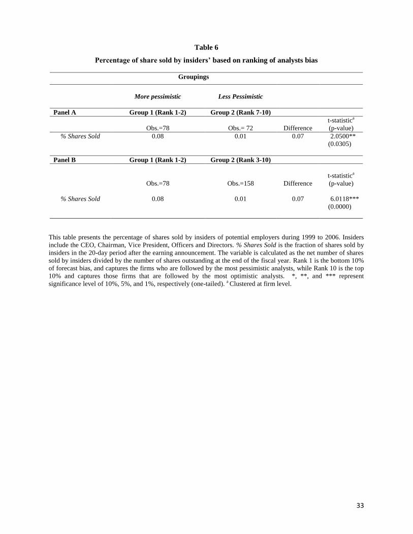
Table 6 presents our analysis. We have a total of 236 observations, which is the number
of individual insiders across all years, who sold their shares during the 20-day period following
the earnings announcement. Panel A compares the mean %Shares Sold for those insiders whose
firms are followed by the top 20% of pessimistic analysts (Group 1: Bias rank 1 to 2) versus
those whose firms are followed by the top 40%8 of optimistic analysts (Group 2: Bias rank 7 to
10). The results indicate that if more pessimistic analysts follow the employer then the insider
sells significantly more of their stock than those firms followed by more optimistic analysts. The
results do not appear to be sensitive to the grouping of firms based on pessimistic versus
optimistic analysts, Panel B reports the results when we group firms based on the top 20% of
pessimistic analysts (Group 1: Bias rank 1-2) compared to all other firms (Group 2: Bias rank 3-
10). Again, we find that insiders whose firm is covered by more pessimistic analysts sell
significantly more shares. These results support our hypothesis that insiders from employers who
have an above average following of analysts with pessimistic forecasts prior to an earnings
announcement, will sell more of their shares. However, we note that the sample of executives is
relatively small and as a result we are cautious to draw strong conclusions from this analysis.
6. Conclusion
This paper investigates how career concerns of analysts that forecast the performance of
potential future employers influence their forecasts. We find evidence of a walk-down to
beatable earnings when forecasting earnings of future employers but not of companies that are
unlikely to be future employers. Moreover, this pattern is more pronounced after the Global
8 There are too few observations in the bottom 20% of firms covered by optimistic analysts for comparison to be fruitful.
Therefore the bottom 40% percentage provides a better comparison in terms of the number of insiders trading (and firms). We
observe that significantly fewer individuals sell shares when the forecast bias is more optimistic, which is also consistent with
managers having a greater trading incentive to sell shares if followed by more pessimistic analysts.

21
Settlement which exacerbated career concerns of analysts by limiting their outside opportunities.
Consistent with career concerns about future employment biasing forecasts we find that
bias in potential future employers’ forecasts lead to favorable career outcomes. No such effect is
found for bias in non-employer forecasts. We also document that consistent with future
employers having the incentive to reward the bias in forecasts, executives of such firms profit
more when analysts have more biased forecasts.
Our paper documents a source of conflict of interest for research analysts that is widely
discussed in other settings, such as auditing. The generalizability of the phenomenon to the
analyst setting is important as it suggests that other information intermediaries might be affected
by such conflicts.

22
References
Abarbanell, J., Bernard, B., 1992. Tests of analysts' overreaction/underreaction to earnings information as
an explanation for anomalous stock price behavior. The Journal of Finance 47, 1181-1207.
Affleck-Graves, J. Davis, L.R., Mendenhall, R.R., 1990. Forecast of earnings per share: Possible sources
of analyst superiority and bias. Contemporary Accounting Research 6, 501-517.
Bailey, W., Li, H., Moa, C.X., Zhong, R., 2003. Regulation fair disclosure and earnings information:
market, analyst, and corporate responses. Journal of Finance 58, 2487-2514.
Barron, O. E., Kim, O., Lim, S., Stevens, D., 1998. Using Analysts' Forecasts to Measure Properties of
Analysts' Information Environment, The Accounting Review 73, 421-433.
Beyer, A., Guttman, I., 2011. The effect of trading volume on analysts’ forecast bias, The Accounting
Review 86, 451-481.
Bradshaw. M.T., 2011. Analysts’ forecasts: What do we know after decades of work? Working paper.
Available at SSRN: http://ssrn.com/abstract=1880339.
Brown, L., Griffin, P., Hagerman, R., Zmijewski, M., 1987. Security analyst superiority relative to
univariate time-series models in forecasting quarterly earnings. Journal of Accounting and Economics 9,
61-87.
Clement, M.B., 1998. Some considerations in measuring analysts’ forecasting performance. Working
paper, University of Texas.
Clement, M.B., 1999. Analyst forecast accuracy: Do ability, resources, and portfolio complexity matter?
Journal of Accounting and Economics 27, 285-303.
Clement, M.B., Tse, S.Y., 2003. Do Investors Respond to Analysts’ Forecast Revisions as if Forecast
Accuracy Is All That Matters?, The Accounting Review 78, 227–249.
Clement, M.B., Tse, S.Y., 2005. Financial analyst’s characteristics and herding behavior in forecasting.
Journal of Finance 60, 307-341.
Cornaggia, J., Cornaggia, K.J., Xia, H., 2015. Revolving doors on Wall Street. Working Paper, Available
at SSRN: http://ssrn.com/abstract=2150998.
Cowen, A., Groysberg, B., Healy, P., 2006. Which types of analysts firms are more optimistic? Journal of
Accounting and Economics 41, 119-146.
Das, S., Levine, C.B., Sivaramakrishnan, K., 1998. Earnings predictability and bias in analysts’ earnings
forecasts. Accounting Review 73, 277-294.
De Bondt, W., Thaler, R., 1990. Do security analysts overreact? The American Economic Review 80, 52-
57.
Dechow, P., Hutton, A., Sloan, R., 2000. The relation between analysts’ forecasts of long-term earnings
growth and stock price performance following equity offerings. Contemporary Accounting Research 17,
1-32.

23
DeHaan, E., Koh, K., Kedia, S., Rajgopal, S., 2012. Does revolving door affect the SEC’s enforcement
outcomes? Rock Center for Corporate Governance at Stanford University Working Paper No. 187;
Stanford University Graduate School of Business Research Paper No. 14-14. Available at SSRN:
http://ssrn.com/abstract=2125560.
Dugar, A., Nathan, S., 1995. The effects of investment banking relationships on financial analysts’
earnings forecasts and investment recommendations. Contemporary Accounting Research 12, 131-160.
Fried, D., Givoly, D., 1982. Financial analysts’ forecasts of earnings: A better surrogate for market
expectations. Journal of Accounting and Economics 4, 85-107.
Flannery, M.J., Kwan, S.H., Nimalendran, M., 2004. Market evidence on the opaqueness of banking
firms’ assets. Journal of Financial Economics 71, 419-460.
Geiger, M., North, D.S., O’Connell, B.T., 2005. The auditor-to-client revolving door and earnings
management. Journal of Accounting, Auditing & Finance 20, 1-26.
Gu, F., Wu, J.S., 2003. Earnings skewness and analysts forecast bias. Journal of Accounting and
Economics 35, 5-29.
Hong, H., Kubik, J.D., 2003. Analyzing the analysts: Career concerns and biased earnings forecasts.
Journal of Finance 58, 313-351.
Hong, H., Kubik, J.D., Solomon, A., 2000. Security analysts’ career concerns and herding of earnings
forecasts. RAND Journal of Economics 31, 121-144.
Hunton, J., McEwen, R., 1997. An assessment of the relation between analysts’ earnings forecast
accuracy, motivational incentives and cognitive information search strategy. The Accounting Review 72,
497-515.
Jackson, A.R., 2005. Trade generation, reputation, and sell-side analysts. Journal of Finance 60, 673-717.
Jacob, J., Lys, T.Z., Neale, M.A., 1999. Expertise in forecasting performance of security analysts. Journal
of Accounting and Economics 28, 41-82.
Ke, B., Yu, Y., 2006. The effect of issuing biased earnings forecasts on analysts’ access to management
and survival. Journal of Accounting Research 44, 965-999.
Kerl, A., Ohlert, M., 2014. Star-analysts’ forecast accuracy and the role of corporate governance.
Available at SSRN: http://ssrn.com/abstract=2195909.
Kim, Y., Lobo, G.J., Wang, M., 2011. Analyst characteristics, timing of forecast revisions and analysts
forecasting ability. Journal of Banking and Finance 35, 2158-2168.
Klein, A., 1990. A direct test of the cognitive bias theory of share price reversals. Journal of Accounting
and Economics 13, 155-166.
Libby, R., Hunton, J.E., Tan, H., Seybert, N., 2007. Relationship incentives and the optimistic/pessimistic
pattern in analysts’ forecasts, Journal of Accounting Research 46, 173–198.

24
Lim, T., 2001. Rationality and analysts’ forecast bias. Journal of Finance 56, 369-385.
Lin, H., McNichols, M.F., 1998. Underwriting relationships, analysts’ earnings forecasts and investment
recommendations. Journal of accounting and economics 25, 101-127.
Lourie, B., 2014. The revolving-door of sell-side analysts: A threat to analysts’ independence? Working
paper. Available at SSRN: http://ssrn.com/abstract=2517957.
Menon, K., Williams, D.D., 2004. Former audit partners and abnormal accruals. The Accounting Review
79, 1095-1118.
Michaely, R., Womack, K.L., 1999. Conflict of interest and the credibility of underwriting analyst
recommendations. Review of Financial Studies 12, 653-686.
Morgan, D.P, 2002. Rating banks: Risk and uncertainty in an opaque industry, The American Economic
Review 92, 874-888.
O’Brien, P., 1988. Analysts’ forecasts as earnings expectations. Journal of Accounting and Economics,
10, 53-83.
O’Brien, P., McNichols, M., Lin, H., 2005. Analyst impartiality and investment banking relations. Journal
of Accounting Research 43, 623-650.
Richardson, S., Tcoh, S., Wysocki, P., 2004. The walk-down to beatable analyst forecasts: The role of
equity issuance and insider trading incentives. Contemporary Accounting Research 21, 885-924.
Schipper, K., 1991. Commentary on analysts’ forecasts. Accounting Horizon, 3, 105-121.

25
Appendix: Variable Definitions
Name Description
DFBijt = The difference between the forecast error for analyst i for firm j at time t and the average forecast error of other analysts
following firm j at time t, scaled by the mean absolute forecast error for firm j at time t. Forecast error is estimated value for
analyst i minus actual value of firm j at time t.
EMPLOYER = An indicator variable which takes the value of one if the forecast is for a company with a sell-side equity department (investment
bank) and zero otherwise.
Earn_Stdjt = Standard deviation of firm j’s prior 5 years earning in year t.
Ln(MVjt) = Natural log of the firm j’s market value at the end of year t .
Ln(BTMjt) = Natural log of the ratio of book value of equity to market value of firm j at the end of year t.
Ln(Followjt) = Analysts following, measured as the natural log of analysts following firm j in year t.
F_Horizonijt
The measure of the time from the forecast date to the end of the fiscal period, calculated as the forecast horizon (days from the
forecast date to the fiscal year-end) for analyst i following firm j in year t minus the average forecast horizon for analysts who
follow firm j in year t, with this difference scaled by the average forecast horizons for analysts following firm j in year t.
dayElapijt
= The measure of the days elapsed since the last forecast by any analysts following firm j in year t, calculated as the days between
analysts i’s forecast of firm j’s earnings in year t and the most recent preceding forecast of firm j’s earnings by any analyst,
minus the average number of days between two adjacent forecasts of firm j’s earnings by any two analysts in year t, with this
difference scaled by the average days between two adjacent forecasts of firm j’s earnings in year t.
frijt
= The measure of analyst i’s forecast frequency for firm j, calculated as the number of firm j forecasts made by analyst i following
firm j in year t minus the average number of firm j forecasts for analysts following firm j in year t, with this difference scaled by
the average number of firm j forecasts issued by analysts following firm j in year t.
Firm_Expijt
= The measure of analyst i’s firm-specific experience, calculated as the number of years of firm-specific experience for analyst i
following firm j in year t minus the average number of years of firm-specific experience for analysts following firm j in year i,
with this difference scaled by the average years of firm-specific experience for analysts following firm j in year t.
Gen_Expijt
= The measure of analyst i's general experience, calculated as the number of years of experience for analyst i following firm j in
year t minus the average number of years of experience for analysts following firm j in year t, with this difference scaled by the
range of years of experience for analysts following firm j in year t.
Num_Coijt
= The measure of the number of companies analyst i follows in year t, calculated as the number of companies followed by analyst i
following firm j in year t minus the average number of companies followed by analysts who follow firm j in year t, with this
difference scaled by the average number of companies followed by analysts following firm j in year t.
Num_Indijt
= The measure of number of industries analyst i follows in year t, calculated as the number of two-digit SICs followed by analyst i
following firm j in year t minus the average number of two-digit SICs followed by analysts who follow firm j in year t, with this
difference scaled by the average number of two-digit SICs followed by analysts following firm j in year t.
Num_Anaijt
= The measure of the analyst’s brokerage size, calculated as the number of analysts employed by the brokerage house employing
analyst i following firm j in year t minus the average number of analysts employed by brokerage houses for analysts following
firm j in year t, with this difference scaled by the average brokerage house size for analysts following firm j in year t.

26
Table 1
Descriptive statistics on analyst and firm characteristics
This table reports descriptive statistics for 3,720 analysts forecast observations from 1999-2006. Analysts and forecast characteristics are derived from
detailed I/B/E/S data. Our sample is analysts that cover both banks and non-banks. We restrict the sample to forecasts issued no earlier than 1 year and no
later than 30 days before the fiscal-year end. And include the last and first forecast issued by the analysts for a particular firm in each sample year. The
firm characteristics are MV, the market capitalization; BTM, the book to market and Follow, the number of analysts covering the firm. The analyst
characteristics are F_Horizon, the number of days from the forecast date to the fiscal year-end; dayElap, the number of days since any analyst’s prior
forecast; Firm_Exp, the analyst’s years of experience forecasting a particular firm’s earnings; Gen_Exp, the analyst’s overall years of forecasting
experience; Num_Co, the number of companies the analyst follows in each year; Num_ind, the number of two-digit SIC industries the analyst follows in
each year, and Num_ana, the number of analysts in the analyst’s brokerage house each year. Panel A reports the descriptive statistics for raw (unscaled)
forecast and analyst characteristics. Panel B reports the descriptive statistic for forecast and analysts characteristics, including forecast bias and earnings
dispersion (DFB, Earn_std), that are scaled to range from 0 to 1 for each firm-year. Panel C reports correlations among scaled characteristics.
Panel A: Distribution of selected raw (unscaled) forecast and analyst characteristics
Variable Description Mean S.D. 25th Percentile Median 75
th Percentile
MV Market Value of the Company (in millions) 35466.09 43134.80 9810.82 18664.82 47503.39
BTM Book to Market of the Company 0.43 0.18 0.32 0.44 0.54
Follow Number of analysts following a firm 21.92 6.46 18.00 22.00 26.00
F_Horizon Forecast Horizon in Days to fiscal year-end 124.78 78.85 85.00 92.00 176.00
dayElap Days from prior forecast revision 5.69 12.84 0.00 1.00 6.00
fr Number of forecast revisions per year 3.30 2.03 2.00 3.00 4.00
Firm_Exp Company specific Experience in Years 4.45 3.74 2.00 3.00 6.00
Gen_Exp General Experience in Years 7.79 5.06 4.00 7.00 11.00
Num_co Number of Companies followed 20.24 12.63 13.00 17.00 23.00
Num_ind Number of two-digit SIC followed 1.90 1.66 1.00 1.00 2.00
Num_ana Number of analysts in Brokerage House 68.65 55.26 23.00 51.00 116.00

27
Panel B: Distribution of scaled forecast and analyst characteristics (n=3720)
Variable Mean S.D. 25th Percentile Median 75
th Percentile
DFB 0.01 0.80 -0.65 0.08 0.63
Earn_Std 0.50 0.35 0.25 0.40 0.65
Ln(MV) 9.93 1.06 9.19 9.83 10.77
Ln(BTM) -0.95 0.51 -1.15 -0.82 -0.61
Ln(Follow) 3.03 0.36 2.89 3.09 3.26
F_Horizon -0.36 0.40 -0.58 -0.51 -0.17
dayElap -0.07 1.86 -1.00 -0.89 0.03
fr 36.91 33.80 16.01 25.13 45.84
Firm_Exp 0.01 0.79 -0.59 -0.21 0.35
Gen_Exp 0.03 0.65 -0.47 -0.11 0.41
Num_Co 0.06 0.58 -0.29 -0.07 0.24
Num_Ind 0.13 0.74 -0.28 -0.13 0.33
Num_Ana -0.01 0.79 -0.66 -0.27 0.59

28
Panel C: Correlations among scaled forecast, firm characteristics and analysts characteristics
Below the diagonal we present correlations for the last forecast bias (DFB) and above the diagonal we present the correlations for the first forecast bias (DFB) all
variables are adjusted for firm-year effects where necessary. The p-values are reported below the correlations in parentheses. All variable definitions are as reported
in the Appendix above. N=3720.
Last DFB Earn_Std Ln(MV) Ln(BTM) Ln(Follow) F_Horizon dayElap Fr Firm_Exp Gen_Exp Num_Co Num_Ind Num_Ana
First DFB
-0.142 -0.036 0.042 0.028 -0.028 0.020 -0.023 0.019 0.015 -0.016 -0.017 0.037
(<0.001) (0.026) (0.009) (0.055) (0.055) (0.168) (0.119) (0.184) (0.289) (0.257) (0.257) (0.012)
Earn_Std 0.076
0.083 0.301 -0.054 0.120 -0.003 -0.220 -0.063 -0.063 -0.062 -0.044 0.018
(<0.001)
(<0.001) (<0.001) (0.001) (<0.001) (0.840) (<0.001) (<0.001) (<0.001) (<0.001) (0.003) (0.235)
Ln(MV) 0.048 0.076 -0.090 0.621 -0.039 -0.028 -0.084 -0.026 -0.039 -0.086 -0.049 -0.007
(0.004) (<0.001) (<0.001) (<0.001) (0.018) (0.093) (<0.001) (0.110) (0.016) (<0.001) (0.003) (0.687)
Ln(BTM) -0.067 0.313 -0.079 0.010 -0.074 -0.013 -0.179 0.034 0.018 -0.045 -0.122 -0.002
(<0.001) (<0.001) (<0.001) (0.555) (<0.001) (0.412) (<0.001) (0.039) (0.270) (0.006) (<0.001) (0.912)
Ln(Follow) -0.060 -0.063 0.618 0.011 -0.033 -0.011 -0.107 -0.017 -0.023 -0.030 0.012 -0.017
(<0.001) (<0.001) (<0.001) (0.508) (0.027) (0.463) (<0.001) (0.247) (0.124) (0.041) (0.402) (0.248)
F_Horizon 0.029 -0.074 0.026 0.114 0.036 -0.080 0.453 0.061 0.065 -0.004 -0.110 0.027
(0.049) (<0.001) (0.106) (<0.001) (0.013) (<0.001) (<0.001) (<0.001) (<0.001) (0.812) (<0.001) (0.068)
dayElap -0.021 -0.02 0.002 0.003 0.014 -0.076 -0.069 0.042 0.090 0.017 0.089 0.029
(0.163) (0.195) (0.884) (0.845) (0.340) (<0.001) (<0.001) (0.005) (<0.001) (0.242) (<0.001) (0.047)
Fr 0.025 -0.195 -0.097 -0.136 -0.083 0.777 -0.044 0.051 0.062 0.049 -0.033 -0.012
(0.094) (<0.001) (<0.001) (<0.001) (<0.001) (<0.001) (0.003) (0.001) (<0.001) (0.001) (0.022) (0.411)
Firm_Exp 0.005 -0.036 -0.035 0.039 -0.011 0.143 -0.003 0.143 0.637 0.169 -0.011 0.059
(0.714) (0.019) (0.029) (0.013) (0.444) (<0.001) (0.828) (<0.001) (<0.001) (<0.001) (0.461) (<0.001)
Gen_Exp -0.007 -0.047 -0.050 0.025 -0.019 0.089 0.045 0.115 0.631 0.301 0.080 0.027
(0.636) (0.002) (0.002) (0.108) (0.200) (<0.001) (0.002) (<0.001) (<0.001) (<0.001) (<0.001) (0.065)
Num_Co -0.001 -0.073 -0.062 -0.077 -0.029 -0.002 0.047 0.026 0.149 0.290
0.469 -0.165
(0.955) (<0.001) (0.001) (<0.001) (0.049) (0.898) (0.002) (0.073) (<0.001) (<0.001)
(<0.001) (<0.001)
Num_Ind 0.017 -0.053 -0.027 -0.159 0.016 0.058 0.098 0.044 -0.027 0.063 0.429
-0.234
(0.261) (0.001) (0.098) (<0.001) (0.256) (<0.001) (<0.001) (0.003) (0.071) (<0.001) (<0.001)
(<0.001)
Num_Ana 0.018 0.009 -0.018 0.004 -0.013 -0.049 0.025 -0.034 0.077 0.039 -0.154 -0.214
(0.236) (0.548) (0.283) (0.822) (0.384) (0.001) (0.096) (0.022) (<0.001) (0.008) (<0.001) (<0.001)

29
Table 2
Comparing analyst forecast bias of bank-analysts first and last yearly earnings forecast
DFBijt = α + 1EMPLOYER + 2Earn_Std+ 3Ln(MVijt) +4Ln(BTMijt) +5Ln(Followijt) + 6F_Horizonijt
+7dayElapijt +8frijt +9Firm_Expit + 10Gen_Expijt + 11Num_Coijt + 12Num_Indijt + 13Num_Anaijt +
14Year F.E + ijt
Analyst Constant Sample Financial Firms Only Sample
(1) (2) (3) (4)
Dependent
Variable
First Forecast
DFB
Last Forecast
DFB
First Forecast
DFB
Last Forecast
DFB
Constant 0.775*** -0.13 -0.107 0.207
(3.24) (-0.78) (-0.45) (1.17)
EMPLOYER 0.176***
-0.151***
0.173* -0.134**
(3.71)
(-3.58)
(1.89) (-2.03)
Earn_Std -0.266***
0.001
-0.230*** 0.046
(-4.47)
(0.02)
(-4.19) (1.19)
Ln(MV) -0.075***
0.081***
-0.039* 0.048***
(-3.11)
(4.30)
(-1.93) (2.76)
Ln(BTM) 0.053
-0.045
0.019 -0.154***
(1.13)
(-1.35)
(0.43) (-4.58)
Ln(Follow) 0.081
-0.215***
0.225*** -0.246***
(0.97)
(-3.60)
(3.18) (-4.33)
F_Horizon 0.232***
-0.004
0.213*** 0.067
(4.04)
(-0.05)
(4.83) (0.99)
dayElap 0.008
-0.005
0.001 -0.007
(0.76)
(-0.63)
(0.15) (-1.19)
fr -0.004***
0.002*
0.001 -0.004***
(-4.28)
(1.87)
(1.15) (-6.20)
Firm_Exp 0.011
0.019
0.022 0.023
(0.35)
(0.78)
(0.80) (1.36)
Gen_Exp 0.05
-0.006
0.040 0.000
(1.09)
(-0.18)
(0.98) (0.01)
Num_Co -0.079
-0.034
-0.065** -0.027
(-1.63)
(-1.11)
(-2.06) (-1.05)
Num_ind 0.028
0.019
-0.000 0.010
(0.69)
(0.92)
(-0.00) (0.38)
Num_ana 0.045
0.042*
0.037 0.030*
(1.58)
(1.86)
(1.52) (1.82)
Year FE Yes
Yes
Yes Yes
Observations 3720
3720
3330 3330
Adjusted R2 6.90%
7.00%
4.20% 5.50% This table reports the ordinary least squares estimation results of the following regression using two sample groups for the years 1999-2006. First forecast is the initial forecast analyst i issued for firm j in year t and last forecast is the last forecast revision analyst i issued for firm j in year t.
Heteroskedasticity-robust standard errors are clustered by analyst. t-statistics are reported in parentheses. *, **, and *** represent significance
level of 10%, 5%, and 1%, respectively (two-tailed). All variable definitions are as reported in the Appendix above.

30
Table 3
Comparing forecast bias of analysts who follow investment banks and non-banks before and after
the Global Settlement
DFBijt = α + 1EMPLOYER + 2Earn_Std+ 3Ln(MVijt) +4Ln(BTMijt) +5Ln(Followijt) + 6F_Horizonijt
+7dayElapijt +8frijt +9Firm_Expit + 10Gen_Expijt + 11Num_Coijt + 12Num_Indijt + 13Num_Anaijt +
14Year F.E + ijt
Before Global Settlement After Global Settlement
First Forecast
Last Forecast
First Forecast
Last Forecast
(1)
(2)
(3)
(4)
Constant 0.926***
-0.014
1.356**
-0.931***
(2.72)
(-0.07)
(2.04)
(-2.68)
EMPLOYER 0.116
-0.128***
0.231**
-0.315***
(1.49)
(-3.31)
(2.28)
(-4.94)
Earn_Std -0.280***
-0.034
-0.249***
-0.022
(-2.87)
(-0.49)
(-3.29)
(-0.44)
Ln(MV) -0.130***
0.124***
-0.03
0.015
(-2.95)
(5.63)
(-0.84)
(0.57)
Ln(BTM) 0.054
-0.098***
-0.074
0.111*
(0.92)
(-2.58)
(-0.82)
(1.73)
Ln(Follow) 0.208
-0.354***
-0.243
0.259**
(1.52)
(-5.45)
(-1.10)
(2.10)
F_Horizon 0.257***
0.225***
0.058
-0.552***
(3.44)
(3.12)
(0.60)
(-3.26)
dayElap 0.019
-0.010
0.006
-0.012
(1.32)
(-1.03)
(0.38)
(-1.15)
fr -0.003**
-0.000
-0.010***
0.008***
(-2.40)
(-0.06)
(-5.30)
(2.72)
Firm_Exp 0.027
0.034
0.033
-0.007
(0.57)
(1.38)
(0.55)
(-0.18)
Gen_Exp 0.056
-0.017
0.006
-0.011
(0.94)
(-0.51)
(0.08)
(-0.23)
Num_co -0.176***
-0.090***
0.041
0.167***
(-3.00)
(-2.73)
(0.51)
(3.25)
Num_ind -0.002
0.044*
-0.096
-0.128***
(-0.04)
(1.86)
(-1.38)
(-2.86)
Num_ana 0.085**
0.037*
-0.013
0.032
(2.01) (1.79) (-0.29) (1.08)
Year FE Yes
Yes
Yes
Yes
N 2303
2303
1417
1417
Adjusted R2 6.10% 11.50% 4.50% 3.0%
This table compares analyst bias before and after the Global Settlement in year 2003 using Analyst Constant sample
from year 1999 to 2006. Before the settlement represents years 1999 to 2003 while after the settlement represents
years 2004 to 2006. First forecast is the initial forecast analyst i issued for firm j in year t and last forecast is the last
forecast revision analyst i issued for firm j in year t. Heteroskedasticity-robust standard errors are clustered by
company and analyst pair. t-statistics are reported in parentheses. *, **, and *** represent significance level of 10%,
5%, and 1%, respectively. All variable definitions are as reported in the Appendix above.

31
Table 4
Brokerage House Status and Job Movement
Panel A: Percentage of analysts who in different status brokerage houses each year
The table presents the percentage of all analysts in I/B/E/S who are categorized as working for
high-status, median-status and low-status brokerage houses.
Brokerage House
Status
High-status
Brokerage House
Median-status
Brokerage House
Low-status
Brokerage House
Year Analyst% Analyst% Analyst%
1999 27.33% 48.17% 24.49%
2000 26.44% 51.57% 21.99%
2001 30.62% 45.26% 24.13%
2002 33.12% 43.88% 23.01%
2003 33.31% 45.12% 21.57%
2004 35.02% 43.28% 21.70%
2005 33.95% 45.15% 20.90%
2006 32.51% 47.58% 19.91%
Overall (1998-2006) 31.53% 46.25% 22.21%
Panel B: Summary statistics of analyst job movement
This table presents the averaged percentage of all analyst and analysts who forecast potential employers in the
I/B/E/S database who move between brokerage houses each year during 1999-2006 and the percentage who
experience various types of job separations in a year averaged over year 1999-2006.
All Analysts
Analysts
forecasting
Employers
% of Analysts Who Change Houses each Year: 6.05%
6.93%
Averaged % of Analysts move up each year 49.39%
51.35%
Averaged % of Analysts move down each year 30.17%
29.73%
Averaged % of Analysts stay high each year 11.32%
12.61%
Averaged % of Analysts stay low each year 9.14%
4.50%
% of Analysts move from High-Status House 16.32%
16.41%
% of Analysts move from Low-Status House 24.61%
15.90%
% of Analysts move from Mid-Status House 59.07% 67.69%

32
Table 5
The effect of forecast bias on job separations of bank analysts and non-bank analysts
Move_statust+1 = 1 BIASijt + 2EMPLOYER + 3 BIASijt * EMPLOYER + 4Gen_Expijt + 5Num_Coijt +
6Low_statusjt +7Medium_statusjt + 8Low_statusjt * EMPLOYER +
9Medium_statusjt * EMPLOYER +10Year F.E + ijt
Dependent Variable= Move_status
Forecast Bias
Variable First Forecast Last Forecast
(1) (2)
Constant 4.544*** 4.607***
(17.17) (18.14)
BIAS 0.172 -0.000
(1.37) (-0.10)
EMPLOYER 0.372 0.655**
(0.82) (2.11)
BIAS*EMPLOYER -0.128 -0.431**
(-0.38) (-2.18)
Gen_Exp -0.006 -0.01
(-0.68) (-1.13)
Num_Co 0.027*** 0.027***
(3.76) (4.22)
Low_status 2.840*** 2.880***
(16.28) (16.61)
Medium_status 1.493*** 1.496***
(11.94) (11.91)
Low_status*EMPLOYER -0.261 -0.471
(-0.39) (-0.75)
Medium_status*EMPLOYER -0.398 -0.559
(-0.83) (-1.50)
Year FE Yes Yes
N 886 886
Pesudo-R2 21.82% 22.30%
This table present estimations from the ordinal probit regression to examine if past forecast optimism from bank and non-bank
analysts have different effect on the likelihood of analyst moves to a higher or lower status brokerage house during 1999 to 2006.
The dependant variable move-statuts equals the value 1 if the analyst in time t moves up one hierarchy of brokerage house status
and the value of 2 if the move up represents a move of two hierarches. If the analyst moves side-ways then it takes the value of
zero. If, however, the analysts moves down one hierarchy then it takes the value of -1, and if the move involves moving down
two hierarches then it takes the value of -2. Consistent with Hong and Kubik (2003), we measures the forecast bias for each firm
the analyst forecasts in year t minus the consensus which we then average across the stocks that the analysts covers which
provides us with a bias measure for analysts i in year t. The BIAS variable is the average this forecast bias in year t and the two
previous years. Analysts who have less than three prior years of experience are excluded. High-status house per year denotes as
brokerage house with house size in the top 3% each year. Low-status house per year denotes as brokerage house size below
average house size each year. Medium-status house is house other than high-status and low-status house. All other variables are
as defined in the Appendix. Heteroskedasticity-robust standard errors are clustered by company and analyst pair. *, **, and ***
represent significance level of 5%, 1%, and 0.1%, respectively (two-tailed).
33
Table 6
Percentage of share sold by insiders’ based on ranking of analysts bias
This table presents the percentage of shares sold by insiders of potential employers during 1999 to 2006. Insiders
include the CEO, Chairman, Vice President, Officers and Directors. % Shares Sold is the fraction of shares sold by
insiders in the 20-day period after the earning announcement. The variable is calculated as the net number of shares
sold by insiders divided by the number of shares outstanding at the end of the fiscal year. Rank 1 is the bottom 10%
of forecast bias, and captures the firms who are followed by the most pessimistic analysts, while Rank 10 is the top
10% and captures those firms that are followed by the most optimistic analysts. *, **, and *** represent
significance level of 10%, 5%, and 1%, respectively (one-tailed). a Clustered at firm level.
Groupings
More pessimistic
Less Pessimistic
Panel A Group 1 (Rank 1-2) Group 2 (Rank 7-10)
Obs.=78
Obs.= 72
Difference
t-statistica
(p-value)
% Shares Sold 0.08 0.01 0.07 2.0500**
(0.0305)
Panel B Group 1 (Rank 1-2) Group 2 (Rank 3-10)
Obs.=78
Obs.=158
Difference
t-statistica
(p-value)
% Shares Sold 0.08 0.01 0.07 6.0118***
(0.0000)