carina huchler - maastricht university · carina huchler aachen, ... 2.3 stand alone editions and...
TRANSCRIPT
AN MCTS AGENT FOR TICKET TO RIDE
Carina Huchler
Master Thesis DKE 15-18
Thesis submitted in partial fulfilmentof the requirements for the degree of
Master of Science of Artificial Intelligenceat the Faculty of Humanities and Sciences
of Maastricht University
Thesis committee:
Dr. Mark H. M. WinandsDr. ir. Jos W. H. M. Uiterwijk
Maastricht UniversityDepartment of Knowledge Engineering
Maastricht, The NetherlandsJuly 8, 2015

Preface
This thesis was written at the Department of Knowledge Engineering of Maastricht University. Thisthesis discusses the implementation of Ticket to Ride in the framework of Monte-Carlo Tree Search. Iwould like to express my thanks to several people. First of all, I would like to thank my supervisor Dr.Mark Winands, for his help during my thesis. He gave me a lot of insightful advice and helpful remarksin writing my thesis. I would also like to thank my boyfriend and fellow student, Emanuel Oster, forhelping me to find my bugs and supporting me throughout the thesis. Finally, I would like to give mygratitude to my family and friends for supporting me during my thesis. I want to thank them not onlyfor playing countless games of Ticket to Ride, but also for giving me moral support.
Carina HuchlerAachen, July 2015

Abstract
The implementation of AI players for games exists at least since 1956 where the first chess player MA-NIAC was implemented. Since this time AI players got more and more attention. For over 14 years nowMonte-Carlo Tree Search (MCTS) got investigated.
This thesis explains Ticket to Ride and the implementation of the game in the Monte-Carlo Tree Search(MCTS) framework. However, the game engine also had to be implemented as well as several enhance-ments for the MCTS algorithm. In the game each player plays a train building company connectingcertain cities as fast as possible. To know which routes to build each player gets certain destinationtickets, which he has to fulfill until the game ends. These destination tickets are only known to the playerhimself.
Ticket to Ride imposes several problems, which have to be considered. The board itself and each possibil-ity a player has each round are known. The game also contains imperfect information, because a playerdoes not necessarily know the cards of his opponents as well as the destination tickets, he needs to ful-fill. The game also contains chance events when a player chooses to draw a card or new destination tickets.
This thesis includes a more detailed description of the rules of Ticket to Ride as well as a calculationof the state-space complexity and game-tree complexity. MCTS, the handling of imperfect informationand chance events and several other enhancements to MCTS are discussed. This enhancements are theSingle-Observer, Multiple-Observer, determinized UCT, voting, progressive unpruning, progressive bias,early termination of the playout step and an ε-rule based strategy.
Since no usable implementation of the game exists, the problems and certain specifications of the imple-mentation have to be discussed as well. The conditions under which the experiments were performed arediscussed as well. The results show that the combination of progressive unpruning and progressive biasworks best with using either the Single-Observer or the Multiple-Observer as its base.
The remaining enhancements were tested as well, but showed no improvement over the combinationof the two progressive approaches. Some enhancements like the determinized UCT, the voting player orthe playout strategy performed even worse than its Single-Observer variant.It is also shown how well imperfect information is handled in the case of Ticket to Ride by comparingit to two different types of the cheating player. Both of them are able to access the knowledge of allplayers. One cheating player also has fixed chance events. The Multiple-Observer has a similar resultwhen playing against the cheating player. Both agents were tested with and without the combination ofprogressive bias and progressive unpruning. Both agents were able to win ∼ 40% of all games. Thereforeboth agents perform well considering their disadvantage.

Contents
Preface iii
Abstract v
Contents vii
1 Introduction 1
1.1 Games and AI . . . . . . . . . . . . . . . . . . . . . . . . . . . . . . . . . . . . . . . . . . 1
1.1.1 History of AI players . . . . . . . . . . . . . . . . . . . . . . . . . . . . . . . . . . . 1
1.1.2 Search Algorithms . . . . . . . . . . . . . . . . . . . . . . . . . . . . . . . . . . . . 1
1.1.3 Success of Monte-Carlo Search as an AI player . . . . . . . . . . . . . . . . . . . . 2
1.2 Ticket to Ride . . . . . . . . . . . . . . . . . . . . . . . . . . . . . . . . . . . . . . . . . . 3
1.3 Problem Statement and Research Questions . . . . . . . . . . . . . . . . . . . . . . . . . . 3
1.4 Thesis Outline . . . . . . . . . . . . . . . . . . . . . . . . . . . . . . . . . . . . . . . . . . 3
2 Ticket to Ride 5
2.1 Rules . . . . . . . . . . . . . . . . . . . . . . . . . . . . . . . . . . . . . . . . . . . . . . . . 5
2.2 Strategy . . . . . . . . . . . . . . . . . . . . . . . . . . . . . . . . . . . . . . . . . . . . . . 7
2.2.1 Counting Cards . . . . . . . . . . . . . . . . . . . . . . . . . . . . . . . . . . . . . . 7
2.2.2 Choosing Destination Tickets . . . . . . . . . . . . . . . . . . . . . . . . . . . . . . 7
2.2.3 Claiming Tracks of Importance to Opponents . . . . . . . . . . . . . . . . . . . . . 8
2.2.4 Building a Continuous Route . . . . . . . . . . . . . . . . . . . . . . . . . . . . . . 8
2.3 Stand Alone Editions and Expansions . . . . . . . . . . . . . . . . . . . . . . . . . . . . . 8
2.4 Complexity . . . . . . . . . . . . . . . . . . . . . . . . . . . . . . . . . . . . . . . . . . . . 8
2.4.1 State-Space Complexity . . . . . . . . . . . . . . . . . . . . . . . . . . . . . . . . . 8
2.4.2 Game-Tree Complexity . . . . . . . . . . . . . . . . . . . . . . . . . . . . . . . . . 9
3 Monte-Carlo Tree Search 11
3.1 Flat Monte-Carlo . . . . . . . . . . . . . . . . . . . . . . . . . . . . . . . . . . . . . . . . . 11
3.2 Monte-Carlo Tree Search . . . . . . . . . . . . . . . . . . . . . . . . . . . . . . . . . . . . . 11
3.3 Upper Confidence Bounds for Trees . . . . . . . . . . . . . . . . . . . . . . . . . . . . . . . 12
3.4 Enhancements . . . . . . . . . . . . . . . . . . . . . . . . . . . . . . . . . . . . . . . . . . 12
3.4.1 Progressive Unpruning . . . . . . . . . . . . . . . . . . . . . . . . . . . . . . . . . . 12
3.4.2 Progressive Bias . . . . . . . . . . . . . . . . . . . . . . . . . . . . . . . . . . . . . 13
3.4.3 Number-of-Visits-Dependent Strategy . . . . . . . . . . . . . . . . . . . . . . . . . 13
3.4.4 Determinization . . . . . . . . . . . . . . . . . . . . . . . . . . . . . . . . . . . . . 13
3.4.5 Cheating MCTS . . . . . . . . . . . . . . . . . . . . . . . . . . . . . . . . . . . . . 13
3.4.6 Single-Observer MCTS . . . . . . . . . . . . . . . . . . . . . . . . . . . . . . . . . . 13
3.4.7 Multiple-Observer MCTS . . . . . . . . . . . . . . . . . . . . . . . . . . . . . . . . 14
3.4.8 Determinized UCT . . . . . . . . . . . . . . . . . . . . . . . . . . . . . . . . . . . . 15
3.4.9 Early Terminations . . . . . . . . . . . . . . . . . . . . . . . . . . . . . . . . . . . . 15
3.4.10 ε-based strategies . . . . . . . . . . . . . . . . . . . . . . . . . . . . . . . . . . . . . 15
viii Contents
4 MCTS in Ticket to Ride 174.1 Nodes . . . . . . . . . . . . . . . . . . . . . . . . . . . . . . . . . . . . . . . . . . . . . . . 17
4.1.1 Actions . . . . . . . . . . . . . . . . . . . . . . . . . . . . . . . . . . . . . . . . . . 174.2 Choosing Destination Tickets . . . . . . . . . . . . . . . . . . . . . . . . . . . . . . . . . . 17
4.2.1 Start of the game . . . . . . . . . . . . . . . . . . . . . . . . . . . . . . . . . . . . . 174.2.2 During the game . . . . . . . . . . . . . . . . . . . . . . . . . . . . . . . . . . . . . 18
4.3 Hidden Information . . . . . . . . . . . . . . . . . . . . . . . . . . . . . . . . . . . . . . . . 184.3.1 Train Cards . . . . . . . . . . . . . . . . . . . . . . . . . . . . . . . . . . . . . . . . 184.3.2 Destination Tickets . . . . . . . . . . . . . . . . . . . . . . . . . . . . . . . . . . . . 19
4.4 Chance . . . . . . . . . . . . . . . . . . . . . . . . . . . . . . . . . . . . . . . . . . . . . . 194.5 Upper Confidence Bounds for Trees . . . . . . . . . . . . . . . . . . . . . . . . . . . . . . . 204.6 Selection Strategy . . . . . . . . . . . . . . . . . . . . . . . . . . . . . . . . . . . . . . . . 20
4.6.1 Heuristic Knowledge . . . . . . . . . . . . . . . . . . . . . . . . . . . . . . . . . . . 204.6.2 Progressive Bias And Unpruning . . . . . . . . . . . . . . . . . . . . . . . . . . . . 21
4.7 Playout Policies . . . . . . . . . . . . . . . . . . . . . . . . . . . . . . . . . . . . . . . . . . 214.7.1 Random . . . . . . . . . . . . . . . . . . . . . . . . . . . . . . . . . . . . . . . . . . 214.7.2 Early Termination . . . . . . . . . . . . . . . . . . . . . . . . . . . . . . . . . . . . 214.7.3 ε-Rule Based Strategy . . . . . . . . . . . . . . . . . . . . . . . . . . . . . . . . . . 21
4.8 Finding the Shortest Path . . . . . . . . . . . . . . . . . . . . . . . . . . . . . . . . . . . . 22
5 Experiments and Results 235.1 AI Players . . . . . . . . . . . . . . . . . . . . . . . . . . . . . . . . . . . . . . . . . . . . . 235.2 Experimental Setup . . . . . . . . . . . . . . . . . . . . . . . . . . . . . . . . . . . . . . . 23
5.2.1 Player Setup . . . . . . . . . . . . . . . . . . . . . . . . . . . . . . . . . . . . . . . 235.2.2 Confidence Bounds . . . . . . . . . . . . . . . . . . . . . . . . . . . . . . . . . . . . 245.2.3 Environmental Setup . . . . . . . . . . . . . . . . . . . . . . . . . . . . . . . . . . . 24
5.3 Single Observer . . . . . . . . . . . . . . . . . . . . . . . . . . . . . . . . . . . . . . . . . . 245.4 Cheating Player . . . . . . . . . . . . . . . . . . . . . . . . . . . . . . . . . . . . . . . . . . 255.5 Enhancements . . . . . . . . . . . . . . . . . . . . . . . . . . . . . . . . . . . . . . . . . . 26
5.5.1 FSO vs. Enhancements . . . . . . . . . . . . . . . . . . . . . . . . . . . . . . . . . 265.5.2 Improving Flat Monte-Carlo with Enhancements . . . . . . . . . . . . . . . . . . . 265.5.3 SO vs. Enhancements . . . . . . . . . . . . . . . . . . . . . . . . . . . . . . . . . . 275.5.4 Combinations . . . . . . . . . . . . . . . . . . . . . . . . . . . . . . . . . . . . . . . 28
5.6 Multiple-Observer MCTS . . . . . . . . . . . . . . . . . . . . . . . . . . . . . . . . . . . . 285.7 Multiple Trees MCTS . . . . . . . . . . . . . . . . . . . . . . . . . . . . . . . . . . . . . . 29
5.7.1 SO vs. Determinized UCT and Voting . . . . . . . . . . . . . . . . . . . . . . . . . 295.7.2 Determinized UCT . . . . . . . . . . . . . . . . . . . . . . . . . . . . . . . . . . . . 295.7.3 Voting . . . . . . . . . . . . . . . . . . . . . . . . . . . . . . . . . . . . . . . . . . . 30
5.8 Early Termination Approach . . . . . . . . . . . . . . . . . . . . . . . . . . . . . . . . . . 315.9 Number of Visits vs. Ratio . . . . . . . . . . . . . . . . . . . . . . . . . . . . . . . . . . . 325.10 Combining PUB with other Approaches . . . . . . . . . . . . . . . . . . . . . . . . . . . . 325.11 Cheating Player vs. Different Agents . . . . . . . . . . . . . . . . . . . . . . . . . . . . . . 335.12 Completing destination tickets . . . . . . . . . . . . . . . . . . . . . . . . . . . . . . . . . 34
6 Conclusion and Future Research 356.1 Thesis summary . . . . . . . . . . . . . . . . . . . . . . . . . . . . . . . . . . . . . . . . . 356.2 Answering the Research Questions . . . . . . . . . . . . . . . . . . . . . . . . . . . . . . . 366.3 Answering the Problem Statement . . . . . . . . . . . . . . . . . . . . . . . . . . . . . . . 376.4 Future Research . . . . . . . . . . . . . . . . . . . . . . . . . . . . . . . . . . . . . . . . . 37
References 39
Chapter 1
Introduction
T his chapter shows the usage of AI in games. It gives a brief introduction tosearch algorithms and the imperfect-information game Ticket to Ride. It alsointroduces the research questions and gives a brief overview of this thesis.
1.1 Games and AI
Over the last few years game-playing agents have become more and more popular. You did not playgames only at home with your friends and family or in your local game shop, but also on your computeror smart phone against other persons all over the world but also against the computer itself.
For playing against the computer, intelligent agents have to be developed. Such agents can havedifferent goals. Such an agent can either play the game as good as possible or it tries to reach a certainkind of level to play against.
These agents were developed for different kinds of games like chess, checkers, Go or poker. The morecommon AI methods are search algorithms. Most of these techniques need an evaluation function. Thebetter such an evaluation function classifies each possible movement, the better it plays the game. Suchevaluation functions can be hard to find.
1.1.1 History of AI players
In 1956 the first chess program, called MANIAC, was able to defeat a novice player in a simplified chessgame (Douglas, 1978). Since then more agents were implemented. The supercomputerDeep Blue wasthe first who was able to defeat a world champion under normal chess tournament conditions against GarryKasparov in 1997. In this match Deep Blue had to play six times, Deep Blue won 3.5–2.5 (Campbell,Hoane Jr., and Hsu, 2002). Around this time people focused more on researching on alternatives for AIengines for other games.
Since then Go has become popular as a research topic. Building a strong engine has turned out to bedifficult, because Go requires a more complex evaluation function than chess. Monte-Carlo Evaluationswas first introduced as a Go player by Brugmann (1993). With this introduction an evaluation functionwas no longer required. 13 years later it was further developed as Monte-Carlo Tree Search (MCTS)(Kocsis and Szepesvari, 2006, Coulom, 2007a). Since then more players were implemented, which wereeven able to compete against humans on expert level. In 2014 the MCTS program Crazy Stone wonagainst the 9 dan player Norimoto Yoda (Wedd, 2015). Norimoto Yoda had a handicap of 4 stones.
1.1.2 Search Algorithms
There are many different search algorithms. A search algorithm is normally used to fulfill an objective.These objectives can have different forms. It is either used to find a path to an objective or to find awinning state. There exist different kinds of search algorithms. In this section a brief overview aboutseven different search algorithms is given: Minimax, αβ-pruning, maxn, Expectimax, Dijkstra, A∗ and

2 Introduction
MCTS.
MinimaxMinimax is an adversarial search algorithm (Von Neumann and Morgenstern, 1944). The algorithm giveseach leaf node a value by using a heuristic function. The algorithm assumes that each player plays asbest as possible. It does so by assuming that the root player or max player maximizes the results, whilethe other player tries to minimize it. At each node the best value according to the belonging player getschosen.
αβ-pruningαβ-pruning improves the Minimax algorithm by pruning branches. A branch is pruned when it is proventhat it cannot influence the upcoming decisions (Knuth and Moore, 1975).
maxn
The maxn algorithm (Luckhart and Irani, 1986) can be used for games with more than two players. Itworks similar to the Minimax algorithm. The biggest difference is that each player has his own value,and that each player maximizes it.
ExpectimaxExpectimax (Michie, 1966) is used for games with a chance element. It changes the Minimax algorithmsuch that it also contains a chance node. The Expectimax algorithm uses the chance element to calculatethe value of a node by multiplying the values of the children with their probabilities.
DijkstraDijkstra is a single agent graph search algorithm (Dijkstra, 1959). It tries to find the path with the lowestcost between a starting node and each other node. Each node, except for the starting node, starts witha cost for the path equal infinity. The algorithm starts at the starting node. It updates all nodes, whichare neighbors and were not visited yet. The updated cost is equal to cost of the distance. It then choosesthe node with the lowest cost and removes it from the list of non-visited nodes. This node is then thecurrent node and all neighbors are updated with the tentative distances.
A∗
A∗ is a single agent pathfinding algorithm. It is used to find the path with the lowest cost between twonodes in a graph. To find such a path it estimates at each node the total cost of movement and tries tokeep it as low as possible. The graph tries to build a way over the nodes, which have the lowest estimatedmovement cost (Hart, Nilsson, and Raphael, 1968).
Monte-Carlo Tree SearchMCTS is a best-first search algorithm (Coulom, 2007a). The algorithm is based on simulating the gamemultiple times and then choosing the most promising option as your move or turn. The algorithm buildsa tree. Each node contains the information for the choosing process.
1.1.3 Success of Monte-Carlo Search as an AI player
One of the first successful Monte-Carlo search was called GIB. It was a bridge player implemented byGinsberg (2001). It competed in the 1998 and the 2000 World Computer Bridge Championships. It wonall games 1998 and all but one in the 2000 championship.A successful implementation of MCTS for an Euro style board game was done by Szita, Chaslot, andSpronck (2010) in Settlers of Catan. The MCTS-10,000 player performed the best with winning 49% ofall played games against several other players.It also has shown some success in handling imperfect information (Cowling, Powley, and Whitehouse,2012). They have tested several games with imperfect information. The games tested were Lord ofthe Rings: The Confrontation (LOTR:C), Dou Di Zhu and the Phantom (4,4,4) game. Theapproach was also tested against humans in the case of LOTR:C. There it was able to win 16 of the 32games played the human player. When the player switched sides the AI player, the AI player was ableto win 14 of the 32 games.
1.2 — Ticket to Ride 3
It also worked well for several other games like Amazons (Lorentz, 2008) and Scotland Yard (Nijssen andWinands, 2012).
1.2 Ticket to Ride
In this thesis the game of Ticket to Ride (TTR) is investigated. Each player takes over the job of a trainbuilding company in America and tries to build train tracks to connect certain cities as fast as possible.Ticket to Ride is a Euro style board game. This means that it uses rather simple rules, has only indirectplayer interaction and no one gets eliminated before the game ends. The game was invented by Alan R.Moon and was published 2004 by Games Of Wonder. It has won several awards and the rules have beentranslated into 11 other languages. The game also has several spin-offs, where you can play the game inother settings with normally only a few more rules. These rules can involve other ways to get victorypoints or special building rules for tracks. Different expansions can change the number of players, buttwo to five players is the most common one.
Each player has destination tickets on his hand, which are unknown to his opponent. A player canalso draw train cards. These cards are also only known to him. Therefore TTR imposes several problemsto the MCTS algorithm. These problems are imperfect information as well as chance events.
1.3 Problem Statement and Research Questions
The goal of this thesis is to implement an MCTS player, which is able to play Ticket to Ride as strongas possible. This leads to the following problem statement:
How can an MCTS player for TTR be developed?
To address the problem statement, this thesis answers the following three research questions.
Are Monte-Carlo methods applicable to Ticket to Ride?It has been shown that Monte-Carlo methods work for many different types of games (Browne et al.,2012), but it has to be tested that it also works for the imperfect-information game Ticket to Ride. Ithas to be tested as well, if MCTS is able to handle the stochastically of TTR.
How can MCTS handle the imperfect-information game in the domain of TTR?Only a little amount of research has been done on handling imperfect-information in MCTS. This makesit an interesting topic to investigate further, how the imperfect information influences the performanceof the game. This will be done, by testing several strategies, which are used to handle imperfect informa-tion. The tested strategies are the Single-Observer, the Multiple-Observer and determinized UCT. Thesestrategies were all introduced by Cowling et al. (2012). The last tested strategy is the voting approach(Nijssen and Winands, 2012).
Which enhancements can improve the MCTS player?It also has to be tested, which enhancements to the implemented player improve its effectiveness. Theenhancements tested in this thesis are progressive unpruning (Chaslot et al., 2008 and Coulom, 2007b),progressive bias (Chaslot et al., 2008) and an ε-rule based strategy.
1.4 Thesis Outline
The outline of this thesis is:
Chapter 1 gives an introduction to the thesis. It starts with introducing the usage of AI in games.This also covers the success of MCTS in different games. Then it gives an overview of different searchalgorithms used in this thesis. Afterwards the general idea and principles of Ticket to Ride are explained.This is followed by the problem statement and research questions.
4 Introduction
Chapter 2 is about Ticket to Ride. The rules of the game are explained and different strategies areshown. It gives a brief introduction of the different stand-alone editions and expansions for the game.The chapter closes with the calculation of the state-space complexity and game-tree complexity.
Chapter 3 gives an introduction in MCTS. It begins with explaining Flat Monte-Carlo. Afterwardsthe enhancement of Flat Monte-Carlo, Monte-Carlo Tree Search, is explained. Then the selection strat-egy Upper Confidence Bounds for Trees is closer analyzed. Then the different enhancements, which wereused in this paper, are introduced. These enhancements contain progressive unpruning and progressivebias as well as determinization, cheating MCTS, Single- and Multiple-Observer, determinized UCT, earlytermination and ε-based strategies.
Chapter 4 shows the connection of Ticket to Ride and MCTS. This chapter shows the special im-plementations, which had to be done, such that Ticket to Ride can be analyzed by MCTS. Thereforethe special node structure is discussed first. Then implementation of choosing destination tickets, animportant part of Ticket to Ride, is explained. Afterwards it is explained how the different types ofhidden information are handled.The chapter also shows the implementation of UCT and explains the specifications of different enhance-ments. Therefore the heuristic knowledge used for progressive bias and progressive unpruning is explained.Different playout policies are also discussed. These playout policies cover the random playout, early ter-mination and the used ε-rule based strategy. It closes with an explanation on how to calculate the shortestpath during a game.
Chapter 5 describes the experiments which are performed. It starts with introducing the generalplayers. Afterwards the experimental setup is shown. This is done by not only showing the setup ofthe different used players, but also by introducing confidence bounds, which is later used to validate theresults. It also gives the specifications of the environmental setup. Afterwards the different experimentsare shortly explained and there results are given and explained.
Chapter 6 concludes the thesis. A brief summary of the results of the thesis is given. Then theresearch questions and the problem statement are answered. The thesis closes with a proposal of futureresearch possibilities.
Chapter 2
Ticket to Ride
T his chapter explains the rules and strategies of Ticket to Ride. It gives a briefoverview over the different standalone editions and expansions of Ticket to Rideand examines its complexity.
2.1 Rules
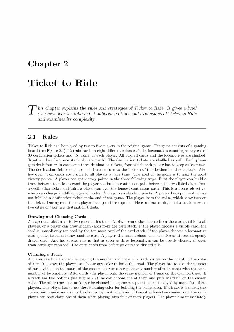
Ticket to Ride can be played by two to five players in the original game. The game consists of a gamingboard (see Figure 2.1), 12 train cards in eight different colors each, 14 locomotives counting as any color,30 destination tickets and 45 trains for each player. All colored cards and the locomotives are shuffled.Together they form one stack of train cards. The destination tickets are shuffled as well. Each playergets dealt four train cards and three destination tickets, from which each player has to keep at least two.The destination tickets that are not chosen return to the bottom of the destination tickets stack. Alsofive open train cards are visible to all players at any time. The goal of the game is to gain the mostvictory points. A player can get victory points in the three following ways. First the player can build atrack between to cities, second the player can build a continuous path between the two listed cities froma destination ticket and third a player can own the longest continuous path. This is a bonus objective,which can change in different game modes. A player can also lose points. A player loses points if he hasnot fulfilled a destination ticket at the end of the game. The player loses the value, which is written onthe ticket. During each turn a player has up to three options. He can draw cards, build a track betweentwo cities or take new destination tickets.
Drawing and Choosing CardsA player can obtain up to two cards in his turn. A player can either choose from the cards visible to allplayers, or a player can draw hidden cards from the card stack. If the player chooses a visible card, thecard is immediately replaced by the top most card of the card stack. If the player chooses a locomotivecard openly, he cannot draw another card. A player also cannot choose a locomotive as his second openlydrawn card. Another special rule is that as soon as three locomotives can be openly chosen, all opentrain cards get replaced. The open cards from before go onto the discard pile.
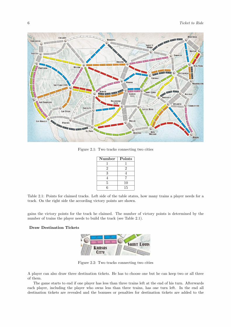
Claiming a TrackA player can build a track by paying the number and color of a track visible on the board. If the colorof a track is gray, the player can choose any color to build this road. The player has to give the numberof cards visible on the board of the chosen color or can replace any number of train cards with the samenumber of locomotives. Afterwards this player puts the same number of trains on the claimed track. Ifa track has two options (see Figure 2.2), he can choose one of them and puts his train on the chosencolor. The other track can no longer be claimed in a game except this game is played by more than threeplayers. The player has to use the remaining color for building the connection. If a track is claimed, thisconnection is gone and cannot be claimed by another player. If two cities have two connections, the sameplayer can only claim one of them when playing with four or more players. The player also immediately
6 Ticket to Ride
Figure 2.1: Two tracks connecting two cities
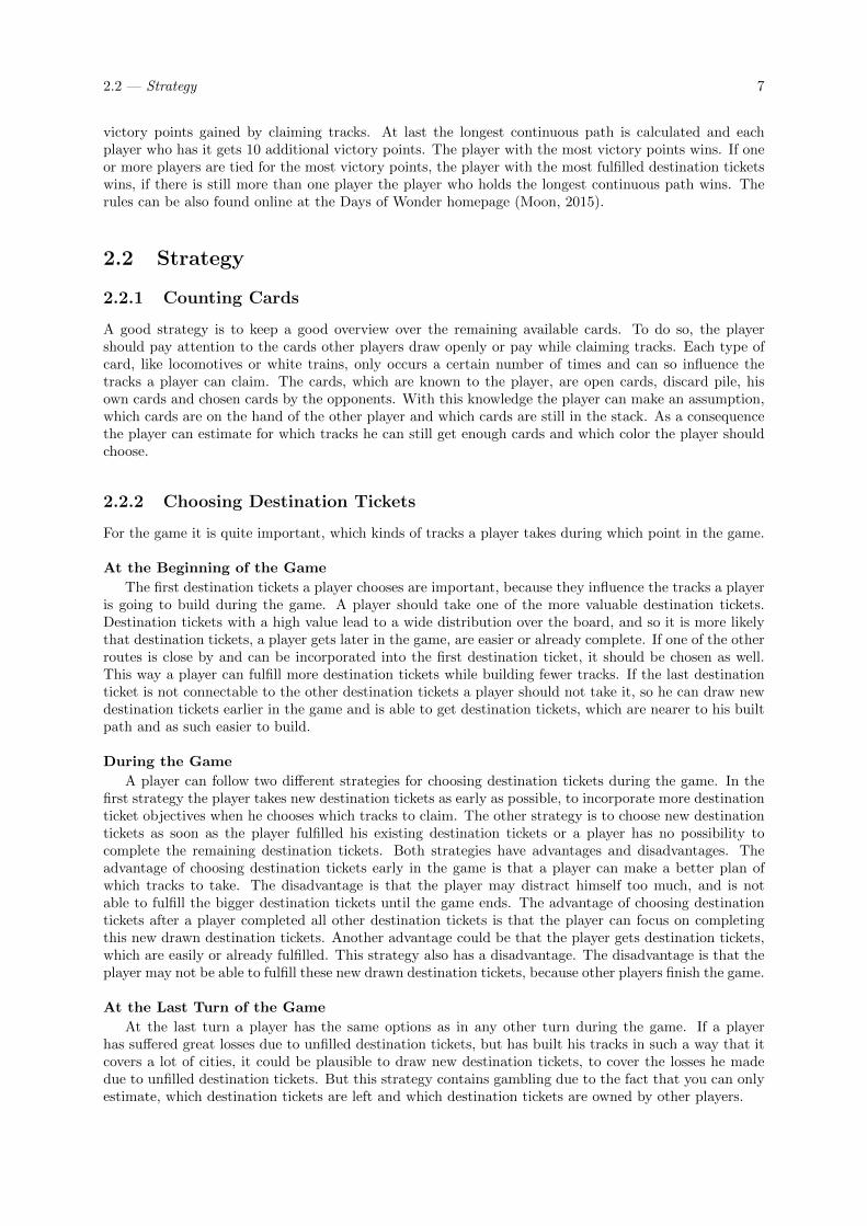
Number Points1 12 23 44 75 106 15
Table 2.1: Points for claimed tracks. Left side of the table states, how many trains a player needs for atrack. On the right side the according victory points are shown.
gains the victory points for the track he claimed. The number of victory points is determined by thenumber of trains the player needs to build the track (see Table 2.1).
Draw Destination Tickets
Figure 2.2: Two tracks connecting two cities
A player can also draw three destination tickets. He has to choose one but he can keep two or all threeof them.
The game starts to end if one player has less than three trains left at the end of his turn. Afterwardseach player, including the player who owns less than three trains, has one turn left. In the end alldestination tickets are revealed and the bonuses or penalties for destination tickets are added to the
2.2 — Strategy 7
victory points gained by claiming tracks. At last the longest continuous path is calculated and eachplayer who has it gets 10 additional victory points. The player with the most victory points wins. If oneor more players are tied for the most victory points, the player with the most fulfilled destination ticketswins, if there is still more than one player the player who holds the longest continuous path wins. Therules can be also found online at the Days of Wonder homepage (Moon, 2015).
2.2 Strategy
2.2.1 Counting Cards
A good strategy is to keep a good overview over the remaining available cards. To do so, the playershould pay attention to the cards other players draw openly or pay while claiming tracks. Each type ofcard, like locomotives or white trains, only occurs a certain number of times and can so influence thetracks a player can claim. The cards, which are known to the player, are open cards, discard pile, hisown cards and chosen cards by the opponents. With this knowledge the player can make an assumption,which cards are on the hand of the other player and which cards are still in the stack. As a consequencethe player can estimate for which tracks he can still get enough cards and which color the player shouldchoose.
2.2.2 Choosing Destination Tickets
For the game it is quite important, which kinds of tracks a player takes during which point in the game.
At the Beginning of the Game
The first destination tickets a player chooses are important, because they influence the tracks a playeris going to build during the game. A player should take one of the more valuable destination tickets.Destination tickets with a high value lead to a wide distribution over the board, and so it is more likelythat destination tickets, a player gets later in the game, are easier or already complete. If one of the otherroutes is close by and can be incorporated into the first destination ticket, it should be chosen as well.This way a player can fulfill more destination tickets while building fewer tracks. If the last destinationticket is not connectable to the other destination tickets a player should not take it, so he can draw newdestination tickets earlier in the game and is able to get destination tickets, which are nearer to his builtpath and as such easier to build.
During the Game
A player can follow two different strategies for choosing destination tickets during the game. In thefirst strategy the player takes new destination tickets as early as possible, to incorporate more destinationticket objectives when he chooses which tracks to claim. The other strategy is to choose new destinationtickets as soon as the player fulfilled his existing destination tickets or a player has no possibility tocomplete the remaining destination tickets. Both strategies have advantages and disadvantages. Theadvantage of choosing destination tickets early in the game is that a player can make a better plan ofwhich tracks to take. The disadvantage is that the player may distract himself too much, and is notable to fulfill the bigger destination tickets until the game ends. The advantage of choosing destinationtickets after a player completed all other destination tickets is that the player can focus on completingthis new drawn destination tickets. Another advantage could be that the player gets destination tickets,which are easily or already fulfilled. This strategy also has a disadvantage. The disadvantage is that theplayer may not be able to fulfill these new drawn destination tickets, because other players finish the game.
At the Last Turn of the Game
At the last turn a player has the same options as in any other turn during the game. If a playerhas suffered great losses due to unfilled destination tickets, but has built his tracks in such a way that itcovers a lot of cities, it could be plausible to draw new destination tickets, to cover the losses he madedue to unfilled destination tickets. But this strategy contains gambling due to the fact that you can onlyestimate, which destination tickets are left and which destination tickets are owned by other players.
8 Ticket to Ride
2.2.3 Claiming Tracks of Importance to Opponents
Another strategy is to claim tracks, which are of great importance to other players. Such a track couldbe a track, which connects two different paths. Opponents then have to estimate of how much value thistrack is for the opponent and if it is worth paying the resources and spending a turn. The advantage ofsuch a move is that the opponent has to spend more resources to connect these two paths and maybedoes not gain the possibility to do so. The disadvantage is that the player has to give up resources of hisown and that the track could be of no to little value for the other player.
2.2.4 Building a Continuous Route
The last strategy is that a player tries to build a track connecting to one of his routes, so that an opponentdoes not build such tracks to the player’s disadvantage. This is especially true for the games with twoor three players, because all tracks can only use one of their connections. In games with more players,more possibilities become available for certain connections. It can be plausible to skip bigger tracks, ifthe player is sure that such tracks are not useful for other players. Most players would not build suchtracks, because the resources, such a move costs, are too high and could be of more value to the playerelsewhere.
2.3 Stand Alone Editions and Expansions
After the first game has been released, four different stand-alone editions were published. The game alsohas six expansions. Two of them would be so called “Mini Expansions”. All other games contain morerules and new content. Most of the expansions cover new maps, like the Europe map in the “Ticket ToRide Europe” stand-alone edition. This stand-alone edition adds a new map, new destination tickets andtrain stations as new game elements. This edition also adds new rules. These cover ferries, tunnels andtrain stations. It also adds a new kind of destination ticket, which a player can only get in the beginning.These destination tickets are the “longest destination ticket” and are worth the most points. One of thenew rules cover train stations, which allow players to use one track that is owned by another player. Thisis a fourth option a player can take on his turn. Each train station is worth 4 victory points at the endof the game, if it is still not placed. Some of the games also have different or more bonus objectives. Oneof them is to have the most fulfilled destination tickets. This thesis only covers the original “USA Map”.
2.4 Complexity
This section discusses the state-space and the game-tree complexity (Allis, 1994) for the two-player variantof Ticket to Ride.
2.4.1 State-Space Complexity
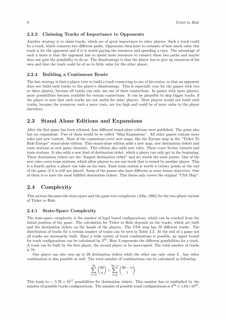
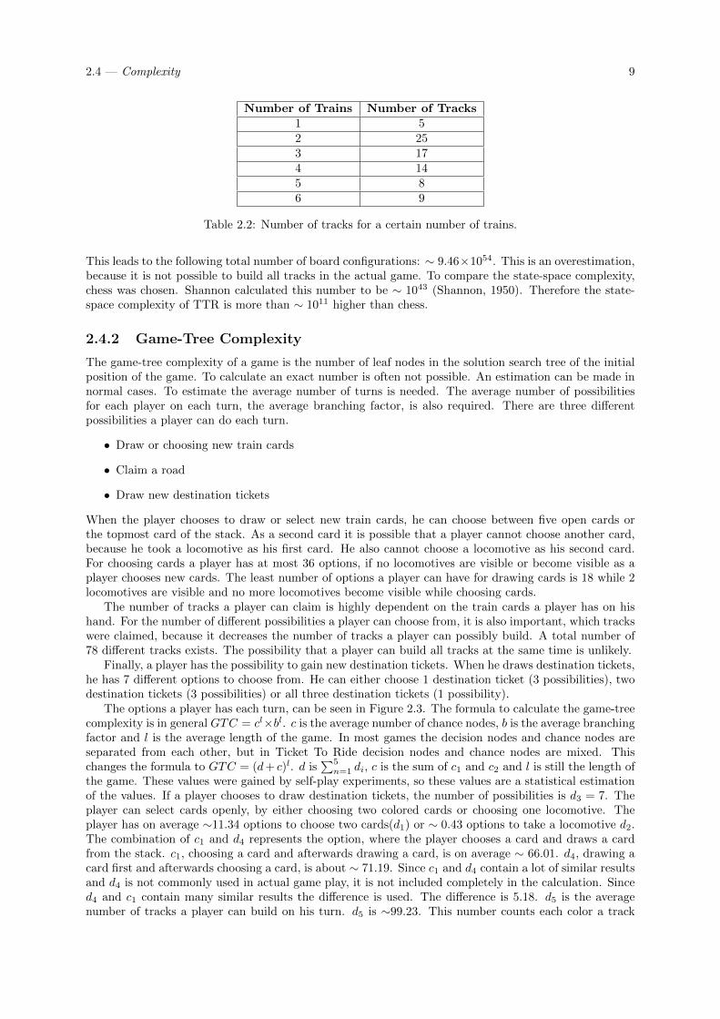
The state-space complexity is the number of legal board configurations, which can be reached from theinitial position of the game. The calculation for Ticket to Ride depends on the tracks, which are builtand the destination tickets on the hands of the players. The USA map has 78 different tracks. Thedistribution of tracks for a certain number of trains can be seen in Table 2.2. At the end of a game notall tracks are necessarily built. Since a wide variety of track combinations is possible, an upper boundfor track configurations can be calculated by 378. Here 3 represents the different possibilities for a track.A track can be built by the first player, the second player or be unoccupied. The total number of tracksis 78.
One player can also own up to 28 destination tickets while the other one only owns 2. Any othercombination is also possible as well. The total number of combinations can be calculated as following:
28∑n=2
(30
n
)×
30−n∑l=2
(30− nl
)This leads to ∼ 5.76 × 10¹⁷ possibilities for destination tickets. This number has to multiplied by thenumber of possible tracks configurations. The number of possible track configurations is 378 ≈ 1.64×1037.
2.4 — Complexity 9
Number of Trains Number of Tracks1 52 253 174 145 86 9
Table 2.2: Number of tracks for a certain number of trains.
This leads to the following total number of board configurations: ∼ 9.46×1054. This is an overestimation,because it is not possible to build all tracks in the actual game. To compare the state-space complexity,chess was chosen. Shannon calculated this number to be ∼ 1043 (Shannon, 1950). Therefore the state-space complexity of TTR is more than ∼ 1011 higher than chess.
2.4.2 Game-Tree Complexity
The game-tree complexity of a game is the number of leaf nodes in the solution search tree of the initialposition of the game. To calculate an exact number is often not possible. An estimation can be made innormal cases. To estimate the average number of turns is needed. The average number of possibilitiesfor each player on each turn, the average branching factor, is also required. There are three differentpossibilities a player can do each turn.
• Draw or choosing new train cards
• Claim a road
• Draw new destination tickets
When the player chooses to draw or select new train cards, he can choose between five open cards orthe topmost card of the stack. As a second card it is possible that a player cannot choose another card,because he took a locomotive as his first card. He also cannot choose a locomotive as his second card.For choosing cards a player has at most 36 options, if no locomotives are visible or become visible as aplayer chooses new cards. The least number of options a player can have for drawing cards is 18 while 2locomotives are visible and no more locomotives become visible while choosing cards.
The number of tracks a player can claim is highly dependent on the train cards a player has on hishand. For the number of different possibilities a player can choose from, it is also important, which trackswere claimed, because it decreases the number of tracks a player can possibly build. A total number of78 different tracks exists. The possibility that a player can build all tracks at the same time is unlikely.
Finally, a player has the possibility to gain new destination tickets. When he draws destination tickets,he has 7 different options to choose from. He can either choose 1 destination ticket (3 possibilities), twodestination tickets (3 possibilities) or all three destination tickets (1 possibility).
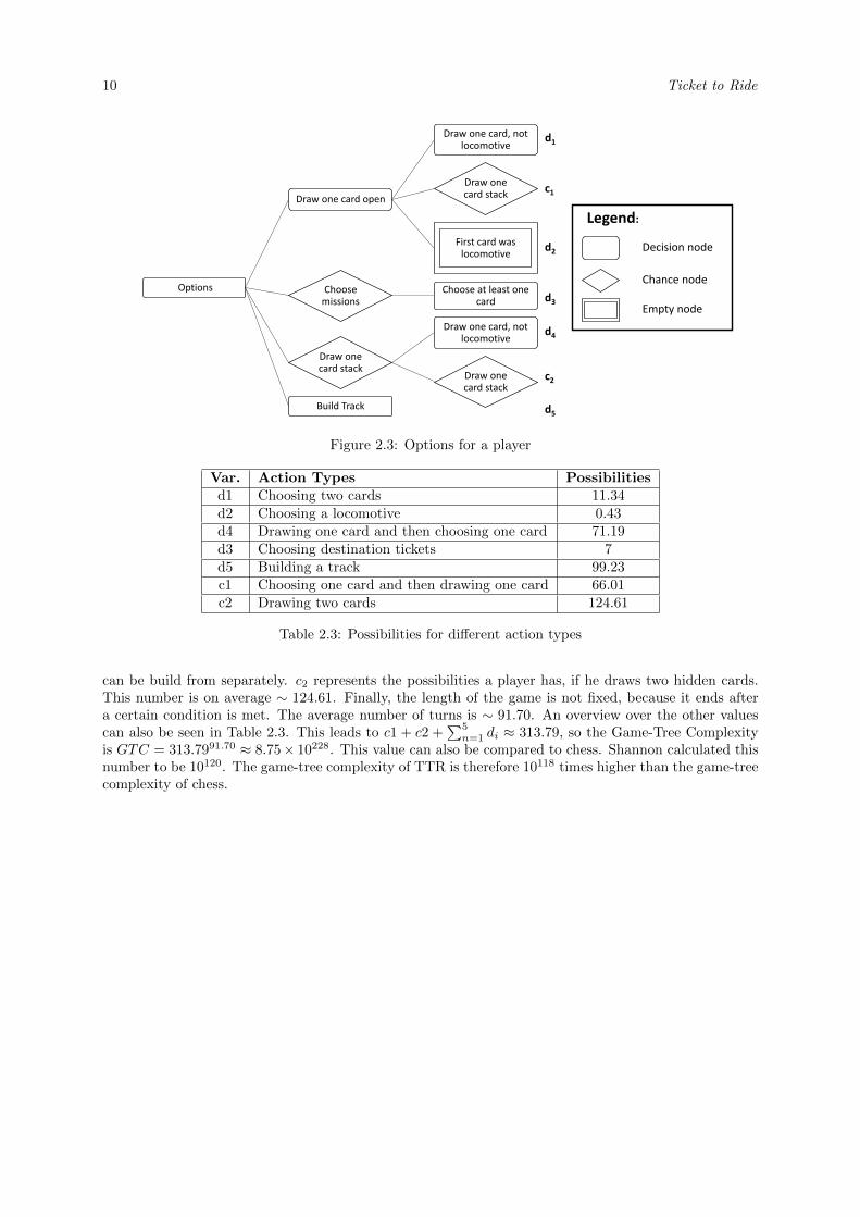
The options a player has each turn, can be seen in Figure 2.3. The formula to calculate the game-treecomplexity is in general GTC = cl×bl. c is the average number of chance nodes, b is the average branchingfactor and l is the average length of the game. In most games the decision nodes and chance nodes areseparated from each other, but in Ticket To Ride decision nodes and chance nodes are mixed. Thischanges the formula to GTC = (d+ c)l. d is
∑5n=1 di, c is the sum of c1 and c2 and l is still the length of
the game. These values were gained by self-play experiments, so these values are a statistical estimationof the values. If a player chooses to draw destination tickets, the number of possibilities is d3 = 7. Theplayer can select cards openly, by either choosing two colored cards or choosing one locomotive. Theplayer has on average ∼11.34 options to choose two cards(d1) or ∼ 0.43 options to take a locomotive d2.The combination of c1 and d4 represents the option, where the player chooses a card and draws a cardfrom the stack. c1, choosing a card and afterwards drawing a card, is on average ∼ 66.01. d4, drawing acard first and afterwards choosing a card, is about ∼ 71.19. Since c1 and d4 contain a lot of similar resultsand d4 is not commonly used in actual game play, it is not included completely in the calculation. Sinced4 and c1 contain many similar results the difference is used. The difference is 5.18. d5 is the averagenumber of tracks a player can build on his turn. d5 is ∼99.23. This number counts each color a track
10 Ticket to Ride
Options
Draw one card open
Draw one card, not locomotive
Draw one card stack
First card was locomotive
Choose missions
Choose at least one card
Draw one card stack
Draw one card, not locomotive
Draw one card stack
Build Track
Decision node
Chance node
Empty node
Legend:
d1
c1
d2
d3
d4
c2
d5
Figure 2.3: Options for a player
Var. Action Types Possibilitiesd1 Choosing two cards 11.34d2 Choosing a locomotive 0.43d4 Drawing one card and then choosing one card 71.19d3 Choosing destination tickets 7d5 Building a track 99.23c1 Choosing one card and then drawing one card 66.01c2 Drawing two cards 124.61
Table 2.3: Possibilities for different action types
can be build from separately. c2 represents the possibilities a player has, if he draws two hidden cards.This number is on average ∼ 124.61. Finally, the length of the game is not fixed, because it ends aftera certain condition is met. The average number of turns is ∼ 91.70. An overview over the other valuescan also be seen in Table 2.3. This leads to c1 + c2 +
∑5n=1 di ≈ 313.79, so the Game-Tree Complexity
is GTC = 313.7991.70 ≈ 8.75× 10228. This value can also be compared to chess. Shannon calculated thisnumber to be 10120. The game-tree complexity of TTR is therefore 10118 times higher than the game-treecomplexity of chess.
Chapter 3
Monte-Carlo Tree Search
T his chapter explains Monte-Carlo Tree Search (MCTS). At first the basis ofMCTS, flat Monte-Carlo, is explained. Then the MCTS algorithm itself is ex-plained. Afterwards the Upper Confidence Bounds for Trees, also called UCT,is shown and the enhancements used for this paper are explained.
3.1 Flat Monte-Carlo
Flat Monte-Carlo is an algorithm which samples the possible actions of a given state (Brugmann, 1993).The algorithm does not need an evaluation function or domain knowledge to work. The algorithm startswith determining the possible actions from the current state of the situation. The algorithm has a timelimit or a certain number of simulations as a restriction for simulating but other restrictions can bepossible as well. The algorithm then simulates a game for each possible movement. It first does thechosen action and then does random movements until the game is finished. This is repeated for allother actions. Each action gets either an equal number of simulations or equal time to do so. Aftereach simulation the action adds one to the number of simulations and one to the number of wins, if thesimulation ended in a win for the current player. In the end the action with the highest win rate is chosenas the best possible action.
3.2 Monte-Carlo Tree Search
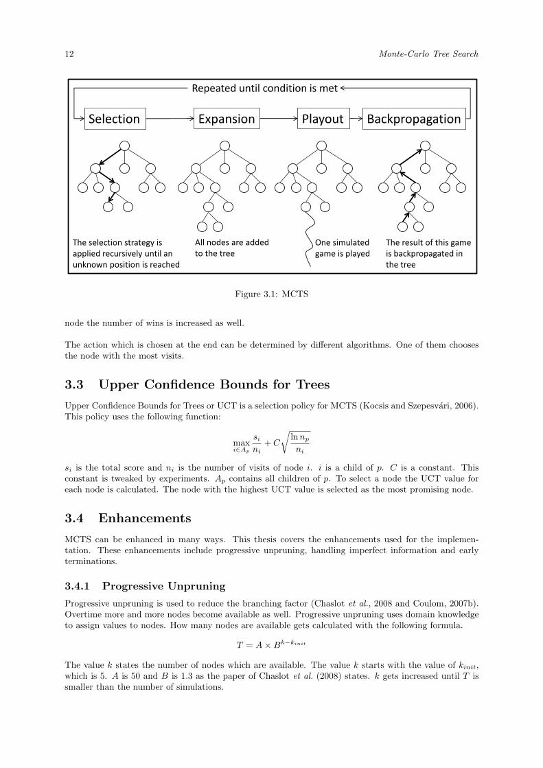
MCTS is an expansion of Flat Monte-Carlo (Coulom, 2007a and Kocsis and Szepesvari, 2006). MCTSuses a tree to save the actions and their results. As first step a root node is created. Afterwards four dif-ferent parts of the algorithm are repeated until a given time has passed or a certain number of iterationsis reached. The four parts are selection, expansion, simulation and backpropagation. These four partscan also be seen in Figure 3.1.
Selection. Starting from the root node, the algorithm selects one of its children by using the cho-sen selection policy. This is repeated until a leaf node is reached.
Expansion. The node, which was chosen in selection, gets a number of children equal to the num-ber of possible actions by the chosen node. Each of these children represents another action from thepossible actions.
Playout. The game uses a policy until the game is finished. This policy can be to choose randomactions, but more informed policies are possible as well.
Backpropagation. The chosen node and its parents get updated with the results of the simulation.The visit counter of each node is increased. If the result is a win for the player belonging to a current
12 Monte-Carlo Tree Search
Repeated until condition is met
Selection Expansion Playout Backpropagation
The selection strategy isapplied recursively until anunknown position is reached
All nodes are addedto the tree
One simulated game is played
The result of this game is backpropagated in the tree
Figure 3.1: MCTS
node the number of wins is increased as well.
The action which is chosen at the end can be determined by different algorithms. One of them choosesthe node with the most visits.
3.3 Upper Confidence Bounds for Trees
Upper Confidence Bounds for Trees or UCT is a selection policy for MCTS (Kocsis and Szepesvari, 2006).This policy uses the following function:
maxi∈Ap
sini
+ C
√lnnpni
si is the total score and ni is the number of visits of node i. i is a child of p. C is a constant. Thisconstant is tweaked by experiments. Ap contains all children of p. To select a node the UCT value foreach node is calculated. The node with the highest UCT value is selected as the most promising node.
3.4 Enhancements
MCTS can be enhanced in many ways. This thesis covers the enhancements used for the implemen-tation. These enhancements include progressive unpruning, handling imperfect information and earlyterminations.
3.4.1 Progressive Unpruning
Progressive unpruning is used to reduce the branching factor (Chaslot et al., 2008 and Coulom, 2007b).Overtime more and more nodes become available as well. Progressive unpruning uses domain knowledgeto assign values to nodes. How many nodes are available gets calculated with the following formula.
T = A×Bk−kinit
The value k states the number of nodes which are available. The value k starts with the value of kinit,which is 5. A is 50 and B is 1.3 as the paper of Chaslot et al. (2008) states. k gets increased until T issmaller than the number of simulations.

3.4 — Enhancements 13
3.4.2 Progressive Bias
Progressive bias is another approach, which is based on heuristic knowledge (Chaslot et al., 2008). Sim-ilarly to progressive unpruning, this approach also tries to guide the selection step into earlier selectingnodes which have a high heuristic value. The enhancement of the selection step is made through anaddition to the UCT formula.
maxi∈Ap
sini
+ C
√lnnpni
+Hi
ni
Hi represents the heuristic knowledge from the action in node i. This value is divided by the number oftimes the node is visited, so the influence of the heuristic knowledge gets smaller over time. Thereforenodes of higher importance get evaluated more closely earlier in the game.
3.4.3 Number-of-Visits-Dependent Strategy
In the two earlier sections progressive unpruning and progressive bias were discussed. Both strategiescan be enhanced by starting at a later point in the simulation. This point is given by a threshold T .The number of visits of the selected node has to be at least equal to this threshold to apply the chosenselection strategy to the node. As long as the threshold is not reached, the selection step uses anothergiven selection strategy. For example this selection strategy could be UCT. The threshold T has to befound empirically.
3.4.4 Determinization
Determinization is an approach to handle imperfect information (Frank and Basin, 1998). Determiniza-tion converts a game of imperfect information into a game with perfect information. It uses the structureof the game and the history of the actual game, to fill in the hidden information. In each iteration, oneof the determinizations is randomly chosen as the current state, which is used for all four parts of theMCTS algorithm.
Determinization has two disadvantages which were explained by Frank and Basin (1998). The firstdisadvantage is called strategy fusion. For each determinization a best action exists. The problem ofstrategy fusion is to find one action which is best for the information set which combines all possible deter-minizations. The second disadvantage non-locality describes the possibility that a determinization maybe unlikely in an actual game. For example, if the opponent has built certain tracks, which would fulfilla certain destination ticket, it is likely that the opponent has this destination ticket. In determinizationit could happen that a player would get another destination ticket, which represents an unlikely state.Even if determinization has several disadvantages, it works for several games like Skat (Buro et al., 2009),Bridge (Ginsberg, 1999) and Phantom Go (Cazenave, 2006).To explain determinization, Ticket to Ride can be used for an example. The train cards from the beginningand the train cards which are drawn from the stack by the opponents are unknown to the player. Thenumber of train cards for each color is known to all players. It is also known which cards are in thediscard pile and which open cards are chosen by the opponents. With this information a stack of cardscan be created. Each opponent then gets a number equal to his hidden cards randomly from this stack.The remaining cards then build the new stack for the current simulation.
3.4.5 Cheating MCTS
Cheating MCTS is used for games with imperfect information. This strategy does not try to handle im-perfect information, but uses all information even if this is normally not possible for the player. CheatingMCTS cannot only be used to handle imperfect information, but it also can be used to gain informationabout the upcoming chance events. This could be done by fixing upcoming chance event.
3.4.6 Single-Observer MCTS
The Single-Observer enhancement is an enhancement for games with imperfect information (Cowl-ing et al., 2012). For each simulation a random determinization is chosen. This enhancement changes theselection step. In the selection step the algorithm disables all moves, which are not possible. It also addsnew moves, if they become available through the new determinization. This can also be seen Figure 3.2.
14 Monte-Carlo Tree Search
A
B
C
Figure 3.2: Possible moves for different determinizations
Selection
Player 1 Player 2
Expansion
Player 1 Player 2
Figure 3.3: MCTS algorithm
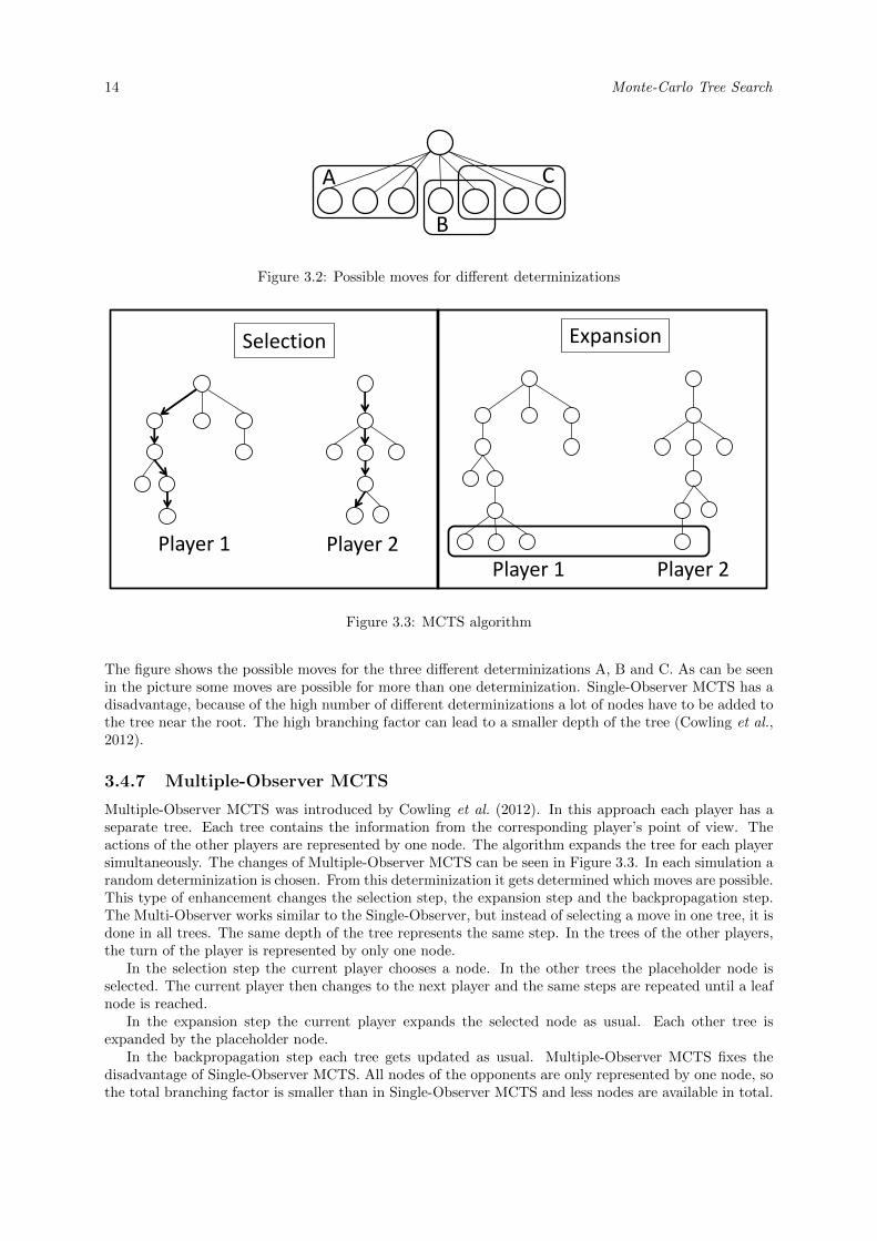
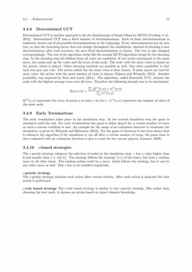
The figure shows the possible moves for the three different determinizations A, B and C. As can be seenin the picture some moves are possible for more than one determinization. Single-Observer MCTS has adisadvantage, because of the high number of different determinizations a lot of nodes have to be added tothe tree near the root. The high branching factor can lead to a smaller depth of the tree (Cowling et al.,2012).
3.4.7 Multiple-Observer MCTS
Multiple-Observer MCTS was introduced by Cowling et al. (2012). In this approach each player has aseparate tree. Each tree contains the information from the corresponding player’s point of view. Theactions of the other players are represented by one node. The algorithm expands the tree for each playersimultaneously. The changes of Multiple-Observer MCTS can be seen in Figure 3.3. In each simulation arandom determinization is chosen. From this determinization it gets determined which moves are possible.This type of enhancement changes the selection step, the expansion step and the backpropagation step.The Multi-Observer works similar to the Single-Observer, but instead of selecting a move in one tree, it isdone in all trees. The same depth of the tree represents the same step. In the trees of the other players,the turn of the player is represented by only one node.
In the selection step the current player chooses a node. In the other trees the placeholder node isselected. The current player then changes to the next player and the same steps are repeated until a leafnode is reached.
In the expansion step the current player expands the selected node as usual. Each other tree isexpanded by the placeholder node.
In the backpropagation step each tree gets updated as usual. Multiple-Observer MCTS fixes thedisadvantage of Single-Observer MCTS. All nodes of the opponents are only represented by one node, sothe total branching factor is smaller than in Single-Observer MCTS and less nodes are available in total.
3.4 — Enhancements 15
3.4.8 Determinized UCT
Determinized UCT is another approach to fix the disadvantage of Single-Observer MCTS (Cowling et al.,2012). Determinized UCT uses a fixed number of determinizations. Each of these determinizations israndomly chosen out of all possible determinizations at the beginning. Every determinization has its owntree, so that the branching factor does not change throughout the simulations. Instead of choosing a newdeterminization after each iteration, the next fixed determinization is chosen. The tree is also changedcorrespondingly. The rest of the algorithm works like the normal MCTS algorithm except for the choosingstep. In the choosing step all children from all roots are combined. If two nodes correspond to the samemove, the nodes add up the visits and the score of the node. The node with the most visits is chosen asthe action, which is played. Other choosing methods are possible as well. One other possibility is thateach tree gets one vote. The action which has the most votes is then chosen. If some moves are tied formost votes, the action with the most number of visits is chosen (Nijssen and Winands, 2012). Anotherpossibility was explored by Fern and Lewis (2011). The algorithm, called Ensemble UCT, chooses thenode with the highest average score over all trees. Therefore the following formula has to be maximized.
QRP (s, a) =
∑iQ
(i)(s, a)× n(i)(s, a)∑i n
(i)(s, a)
Q(i)(s, a) represents the score of action a in state s in tree i. n(i)(s, a) represents the number of visits ofthe same node.
3.4.9 Early Terminations
The early termination takes place in the simulation step. In the normal simulation step the game issimulated until the end. For early terminations the game is either played for a certain number of turnsor until a certain condition is met. An example for the usage of an evaluation function to terminate thesimulation, is given by Winands and Bjornsson (2010). For the game of Amazons it has been shown thatit enhances the algorithm if the simulation is cut off after a certain number of turns, the game state isthen evaluated with an evaluation function to give a result for the current playout (Lorentz, 2008).
3.4.10 ε-based strategies
The ε-greedy strategy enhances the selection of nodes in the simulation step. ε has a value higher than0 and smaller than 1 (ε ∈]0, 1[). The strategy follows the strategy (1-ε) of the times, but does a randommove in all other times. The random action could be a move, which follows the strategy, but it can beany other move as well. This ε has to be tweaked empirically.
ε-greedy strategyThe ε-greedy strategy analyses each action after certain criteria. After each action is analyzed the bestaction is performed.
ε-rule based strategy The ε-rule based strategy is similar to the ε-greedy strategy. But rather thanchoosing the best node, it chooses an action based on expert domain knowledge.

16 Monte-Carlo Tree Search
Chapter 4
MCTS in Ticket to Ride
T his chapter explains integration of MCTS in Ticket to Ride.
4.1 Nodes
A node has to know all its children as well as the children which are possible at the moment. For eachinformation set different determinizations exist. Due to this it can happen that a player can build a trackin one determinization, but not in another one. A node also has to save the number of visits and wins.
4.1.1 Actions
A node in Ticket to Ride has to represent three different actions a player can take, but it has only torepresent one of these actions at a time.
• Choose and/or draw cards
• Choose destination tickets
• Build one track
Each of these actions has to be represented in a special way. The action of choosing or drawing a cardis represented by a number. This value represents the card’s position within the visible train cards. Ifthe value is equal to the size of the array, a card is drawn. Choosing a destination ticket can also berepresented by a number. For this the node can save up to three values between 0 and 2. If a destinationticket is chosen, the player gets three destination tickets to choose from. The saved values represent theposition of the destination tickets in this list. The last action is to build a track. This action can also berepresented by a number. Each track has a certain ID by which it can be referenced. If a node representsthis type of action, it is necessary to know which colors can be used by the player to build this track. Allactions need a list to store information, so each different type of action can reuse that list. The actionalso stores information about its type and the player who performs it.
4.2 Choosing Destination Tickets
This section describes the process of choosing destination tickets at the beginning and during the game.The tickets at the start of the game are evaluated and chosen directly. The tickets, which are chosenduring the game, are checked, if they are fulfilled and then evaluated with MCTS.
4.2.1 Start of the game
At the start of the game each player is handed three destination tickets. From these tickets the playerhas to choose at least two. If one ticket is not chosen, it gets returned to the bottom of the destination
18 MCTS in Ticket to Ride
tickets stack. These tickets have to be chosen right away. The selection of at least two tickets can beseparated in several steps. The engine always chooses only two tickets. First the destination tickets theplayer got, are evaluated by the number of points a player scores, if they fulfill them. The destinationticket with the highest score is chosen as the first destination ticket. The tracks on the shortest path ofthis destination ticket are virtually built for the further analysis of the two remaining destination tickets.
The shortest path for the remaining two destination tickets are calculated separately. These paths arethen compared to the path of the already chosen destination ticket. Each track, which exists in both lists,is removed. The number of removed tracks is counted for each destination ticket separately. After eachtrack is checked, the destination ticket, which shares the most tracks with the first destination ticket, ischosen. If both destination tickets have removed the same number of tracks, the destination ticket withfewer tracks to build is chosen. If two paths share some or most of their track, a longer continuous pathcan be built. This helps later in the game to integrate more destination tickets in the network of trainsa player has.
If no distinct answer is found, the destination ticket with the higher value is chosen. In the casethat both destinations have the same value, the last destination ticket is chosen. This ticket can still beconsidered random, because the destination tickets a player get are random and as such are in a randomorder.
4.2.2 During the game
As soon as all destination tickets are fulfilled, a player should draw new destination tickets, especially ifthe end of the game is not imminent. The possible combinations of destination tickets, if he takes newdestination tickets first, is at least 2925. The general formula to calculate this number is
total =(30− nr)!
(27− nr)!× 3!
nr represents the number of destination tickets, which are known by the player. The value 2925 representsa two-player game, where each player has chosen his starting hand. The calculation of this number alsoconsiders to have no knowledge about the destination tickets of the opponent other than the number. nris in this case equal 6.
If the opponent’s destination tickets are known, nr = 3, the number of combinations is still 2024.Drawing destination tickets is unreliable, if a player tries to predict which destination tickets he wouldget. If a player has all his destination tickets fulfilled, new destination tickets are drawn immediately, ifit is not his last round of the game.
The player draws three new destination tickets as his next action. From these tickets he has to takeat least one, but he can keep any number. Unfulfilled tickets still give negative points at the end of thegame.
All destination tickets are checked, if they are fulfilled, because a player built tracks, which belongto this destination ticket. The unfulfilled drawn tickets generate the new actions by creating a separateaction for each possible combination. Up to seven different actions are possible when no destination ticketwas already fulfilled, otherwise fewer combinations are possible. To these actions the fulfilled destinationtickets are added, such that the destination tickets are added to the player’s hand when the action isselected. If at least one of the drawn destination ticket is fulfilled, an action which includes only fulfilleddestination tickets, is created as well. These actions are then evaluated with MCTS.
4.3 Hidden Information
In Ticket to Ride it is unknown which cards were secretly drawn by the opponents. It is also unknownwhich destination tickets the opponents have chosen. These are two different types of hidden informationand therefore have to be handled differently. The process of filling in this hidden information is alsocalled determinization.
4.3.1 Train Cards
The stack and train cards drawn from it by the opponent are unknown to the player. These train cardscan be estimated. This process is called determinization.
4.4 — Chance 19
To find out these train cards, the player can use the deck of train cards. The deck represents all traincards, which are on the hands of all players, open-lying, the stack and the discard pile. All cards, whichwere chosen openly, the cards to choose from, and are on the discard pile are removed from the deck. Fora determinization for a certain player, his unknown cards have to be assigned. The remaining cards haveto be in the stack or on the opponents’ hands. This deck is called hidden cards for the rest of this thesis.It is possible to narrow down the cards of the opponent even further. As soon as the stack is empty, allcards, which are on the hands of all opponents, are known to the player. All cards are now either in thediscard pile, open-lying or on the hands of a player. In a game with two people a player knows for certainwhich cards are owned by the opponent. In a game with more than two players, a player only knows thecards that have to be on the hands of all opponents.As an example a two-player game of TTR is considered, which both players have drawn cards directlyfrom the stack, so these cards are only known by the players. Player 1 has drawn two red and a yellowcard and Player 2 has drawn a green and also a yellow card. As soon as the stack is empty, all cardsof the opponent are known by the player. Player 1 would need to look in the discard pile and at theopen-lying cards, eliminate these cards from the possible deck of cards, and then do the same with hisown cards and the cards which were chosen by the opponent openly. The remaining cards have to be thecards which were secretly drawn by the opponent. This procedure is easily adaptable for more than twoplayers, but then a player has to assign these cards randomly to the hands of his opponents.In the determinization each opponent gets assigned cards equal to his number of cards which he hasdrawn from the stack. If some of these cards are known, because the stack was empty at one point,this knowledge is used first. The remainder of cards is randomly assigned from the hidden cards. Theremaining hidden cards are then shuffled and become the new stack. To use the example from above,Player 1 knew that Player 2 has a green and a yellow card on his hand. In the next round he drewanother card from the stack. In the determinization a green and a yellow card is assigned to the hand ofPlayer 2, because he has not played these cards yet. He also gets a random card from the hidden cards,because Player 1 has no information about this card. The remaining hidden cards become the new stack.
4.3.2 Destination Tickets
Each player also has destination tickets. These destination tickets are known to the player, but unknownto his opponent. The number of destination tickets is also known. Each destination ticket is unique. Agame has always the same destination tickets, so the destination tickets which exist are known as well.The destination tickets of the player are subtracted from all possible destination tickets. The remainingdestination tickets are possible for the opponents. Three different strategies have been implemented todetermine which destination tickets an opponent could have. The first strategy randomly assigns thedestination tickets. The last two strategies use the tracks the opponent has built. The destination ticketswhich would be fulfilled get selected. Both strategies use these destination tickets as the destinationtickets the opponent has. If these destination tickets are more than the opponent should have, thesecond strategy takes the destination tickets with the highest value. The third strategy chooses thesedestination tickets randomly. If the opponent has too few destination tickets, the second strategy takesthe destination tickets with the lowest value from the remaining destination tickets. The third strategychooses these destination tickets randomly from the remaining ones.
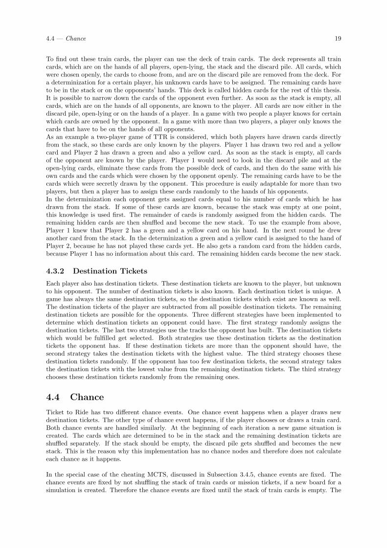
4.4 Chance
Ticket to Ride has two different chance events. One chance event happens when a player draws newdestination tickets. The other type of chance event happens, if the player chooses or draws a train card.Both chance events are handled similarly. At the beginning of each iteration a new game situation iscreated. The cards which are determined to be in the stack and the remaining destination tickets areshuffled separately. If the stack should be empty, the discard pile gets shuffled and becomes the newstack. This is the reason why this implementation has no chance nodes and therefore does not calculateeach chance as it happens.
In the special case of the cheating MCTS, discussed in Subsection 3.4.5, chance events are fixed. Thechance events are fixed by not shuffling the stack of train cards or mission tickets, if a new board for asimulation is created. Therefore the chance events are fixed until the stack of train cards is empty. The
20 MCTS in Ticket to Ride
discard pile is then shuffled randomly to create a new stack. From this point the chance events are nolonger known to the player regarding the discard pile. The destination ticket stack gets never shuffled,so this information is always known to the cheating MCTS.
4.5 Upper Confidence Bounds for Trees
Upper Confidence Bounds for Trees (UCT) as described in Section 3.3 needs some adjustment before itcan be implemented. Two different problems have to be further examined. The first problem happensif a node was never visited yet. The second problem occurs if more than one child has the same UCTvalue.
To handle the first problem, the method to calculate the UCT value returns 1.For the second problem, a random value is added to the UCT value. Therefore a random value
between 0 and 1 is divided by 10k. This random value does not have an influence on the actual UCTvalue, but allows to differentiate between the different nodes.
4.6 Selection Strategy
This section describes the different strategies, which were implemented to improve the selection step.The used heuristic knowledge is explained first, because the selection strategies are based on it.
4.6.1 Heuristic Knowledge
Progressive bias and progressive unpruning depend on heuristic knowledge. Therefore each action gets acertain value. These values need some game knowledge which has to be calculated. Two different typesof information are important here. The first information contains all tracks, which still have to be built,to fulfill the destination tickets of a player. The second information stores the train colors, which areneeded for the tracks, to fulfill the destination tickets of a player.
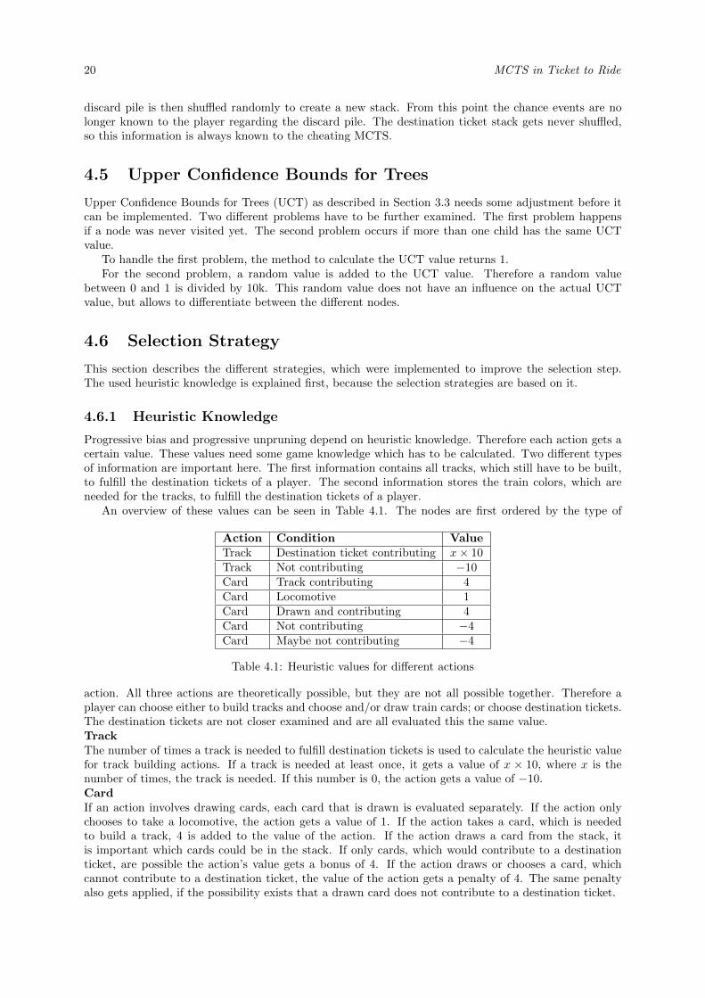
An overview of these values can be seen in Table 4.1. The nodes are first ordered by the type of
Action Condition ValueTrack Destination ticket contributing x× 10Track Not contributing −10Card Track contributing 4Card Locomotive 1Card Drawn and contributing 4Card Not contributing −4Card Maybe not contributing −4
Table 4.1: Heuristic values for different actions
action. All three actions are theoretically possible, but they are not all possible together. Therefore aplayer can choose either to build tracks and choose and/or draw train cards; or choose destination tickets.The destination tickets are not closer examined and are all evaluated this the same value.TrackThe number of times a track is needed to fulfill destination tickets is used to calculate the heuristic valuefor track building actions. If a track is needed at least once, it gets a value of x × 10, where x is thenumber of times, the track is needed. If this number is 0, the action gets a value of −10.CardIf an action involves drawing cards, each card that is drawn is evaluated separately. If the action onlychooses to take a locomotive, the action gets a value of 1. If the action takes a card, which is neededto build a track, 4 is added to the value of the action. If the action draws a card from the stack, itis important which cards could be in the stack. If only cards, which would contribute to a destinationticket, are possible the action’s value gets a bonus of 4. If the action draws or chooses a card, whichcannot contribute to a destination ticket, the value of the action gets a penalty of 4. The same penaltyalso gets applied, if the possibility exists that a drawn card does not contribute to a destination ticket.

4.7 — Playout Policies 21
Drawing two cards which help to build such tracks gets a value of 8. Choosing or drawing only onecard that will contribute to the possible tracks will give an action a value of 0. If only a locomotiveis chosen, the action gets a value of 1. If an action chooses two cards, which might not or does notcontribute to destination ticket tracks, the action gets a value of -8.
4.6.2 Progressive Bias And Unpruning
Progressive bias and progressive unpruning use the heuristic knowledge to select nodes during the selectionstep. The values are calculated once for each node. Progressive bias uses heuristic knowledge during theUCT calculation, while progressive unpruning uses the value to prune children.
A threshold for the number of visits can be given. This threshold has to be reached in a parentnode, before progressive unpruning or progressive bias is used on its children. Otherwise it uses anotherselection strategy such as UCT. This strategy is given at the initialization.
4.7 Playout Policies
The further discussed policies were implemented to improve the simulation step. This section discussesthe random policy, the early termination policy and the strategy policy.
4.7.1 Random
The most common playout policy is the random playout. All actions a player can take are determined andone of them is randomly chosen. Due to the fact that the outcome of acquiring new destination tickets ishighly unpredictable, each action which chooses new destination tickets is not added as a possible moveand only other actions can be chosen.
4.7.2 Early Termination
As discussed in Subsection 3.4.9 the playout can be terminated earlier than the end of the game. If theearly termination is used, the playout ends after 45 moves which is about half of a normal game. Thegame is then rated as a regular game. This means it is either rated as a win or a loss for the correspondingplayer.
4.7.3 ε-Rule Based Strategy
Instead of doing random plays during the simulation step, these steps can follow certain rules. This iscalled a playout strategy. In this master thesis an ε-rule based strategy is used. The playout strategyfollows the strategy (1− ε) of the times and does a random play ε of the times.
Each round, if the playout strategy is used, the tracks, which are needed to fulfill the current desti-nation tickets are calculated and saved for all players. Each player has his own list with his own tracks.Each round the playout strategy looks for the track, which needs the highest number of train cards andbelongs to the list of the current player. If a buildable track is found, which needs six cards, the selectionends early and the action to build the track is performed. If no track is found, the playout compares thebuildable tracks to the tracks of the other player. The strategy then searches for the smallest track forwhich the player has the necessary cards. If a track is found, which needs only one card, the track isbuilt immediately. After all tracks were compared and no track was found that fits the criteria, cards aredrawn or chosen. All possibilities, which either choose or draw up to two cards, are calculated and one ofthem is randomly performed. If no cards were drawn or chosen, one of the tracks which is buildable, israndomly executed. If the playout needs to select a random action, all possible actions except choosingnew destination tickets are found. One of these actions is then randomly selected and afterwards per-formed.
Fulfilling destination tickets has the advantage that the simulation is more accurate, because this wouldhappen in the actual game as well. It is also preferred to build tracks for the player itself over tracks,which the opponent needs. The reason for building tracks, which are needed by opponents, is that it can

22 MCTS in Ticket to Ride
be helpful to block opponents to fulfill their destination tickets. However, a player only wants to investas little as possible in such a strategy. Building tracks also ends the simulation faster, and so a highernumber of simulations is possible.
This type of playout policy has another option for an early termination. The termination should beperformed, if the list of tracks to build is empty. This is a point during the game where new destina-tion tickets are chosen. It is a good point to end the playout, because choosing destination tickets in asimulation is unpredictable (see Subsection 4.2.2). Therefore no meaningful results can be obtained fromchoosing new destination tickets during the playout strategy and the current game situation can still beevaluated.
4.8 Finding the Shortest Path
During the game the calculation of the shortest path is used for different strategies like progressive bias,progressive unpruning or the playout strategy. The strategies depend on the knowledge to know, whichtracks have to be built to accomplish destination tickets. Dijkstra and A∗, briefly discussed in Section1.1.2, were used to find the shortest path. The infrastructure of railroads or map of tracks is stored as anundirected graph. In this graph the nodes represent the cities and the edges represent the tracks. Thecost of an edge is equal to the number of trains a player needs to build that track. For further analysisit is also important to know, if a track was already built and if so, which player build the track.
Before a game starts, the graph is evaluated and the lowest connection cost from one city to each othercity is calculated. After this is done for all cities, this information is stored for later analysis. A∗ usesthe stored information to plot the shortest path from one city to another. Therefore Dijkstra was usedas an underestimation for A∗. Instead of an heuristic function the A∗ algorithm uses the evaluation ofthe Dijkstra algorithm as its heuristic knowledge. The A∗ algorithm considers, if a track was built bythe player the information is considered to find a shorter path. The algorithm also takes into account, ifa track was built by an opponent. A∗ then tries to find an alternative shortest path.
The algorithm does not consider, if the player actual has enough resources to build all tracks. Thismeans, that if a player should not own enough trains, which he needs to claim a track, a shortest pathwould be returned.

Chapter 5
Experiments and Results
T his chapter shows the different AI players, which were implemented. It alsoexplains the setup of the experiments. Then the different experiments are ex-plained and the results are analyzed.
5.1 AI Players
In general, five different types of AI Players were implemented. The five players are Cheating Player,Single Observer, Multiple-Observer MCTS, determinized UCT and voting. All of these players can beenhanced by the different enhancements discussed in Chapter 4.
A special player, which was implemented, is a combination of progressive unpruning and progressivebias. The agent works in the following way. First the nodes are pruned with progressive unpruning.Afterwards the node is selected with progressive bias. All information about progressive unpruning canbe found in Subsection 3.4.1. Progressive bias has been explained in Subsection 3.4.2.
5.2 Experimental Setup
In most cases, each experiment was performed at least 200 times. If an experiment included more than200 games, this information is included in the experiment. Each player started in an equal number ofgames, so if 200 games were played, each player started 100 times. If it is not otherwise stated, the MCTSalgorithm got 2 seconds of thinking time. The other thinking time, which has been used, is 4 seconds.
This section will also discuss the undefined parameters of different players. Confidence bounds areexplained as well. Next, the environment in which the experiments were performed is shown.
5.2.1 Player Setup
The used values for the different constants are discussed below. All agents are simulating until the endof the game, if not otherwise stated.
The UCT algorithm, see Section 3.3, uses a C value of√
2. The progressive unpruning (see Subsec-tion 3.4.1) and progressive bias (see Subsection 3.4.2) approaches have a threshold of 0. This means thatboth strategies directly start their approach after a node is selected the first time. The constants, whichare used to determine how many nodes are not pruned in the progressive unpruning selection step, wereset as discussed in Subsection 3.4.1. Therefore A was set to 25 and B to 1.3. The value for kinit is 5.The heuristic value of progressive bias is not modified. The voting and determinized UCT approachesshuffle the card stack each time when a new board for a simulation is created. This way the cards inthe hands of the other player are always the same, but the train card stack and the mission stack are
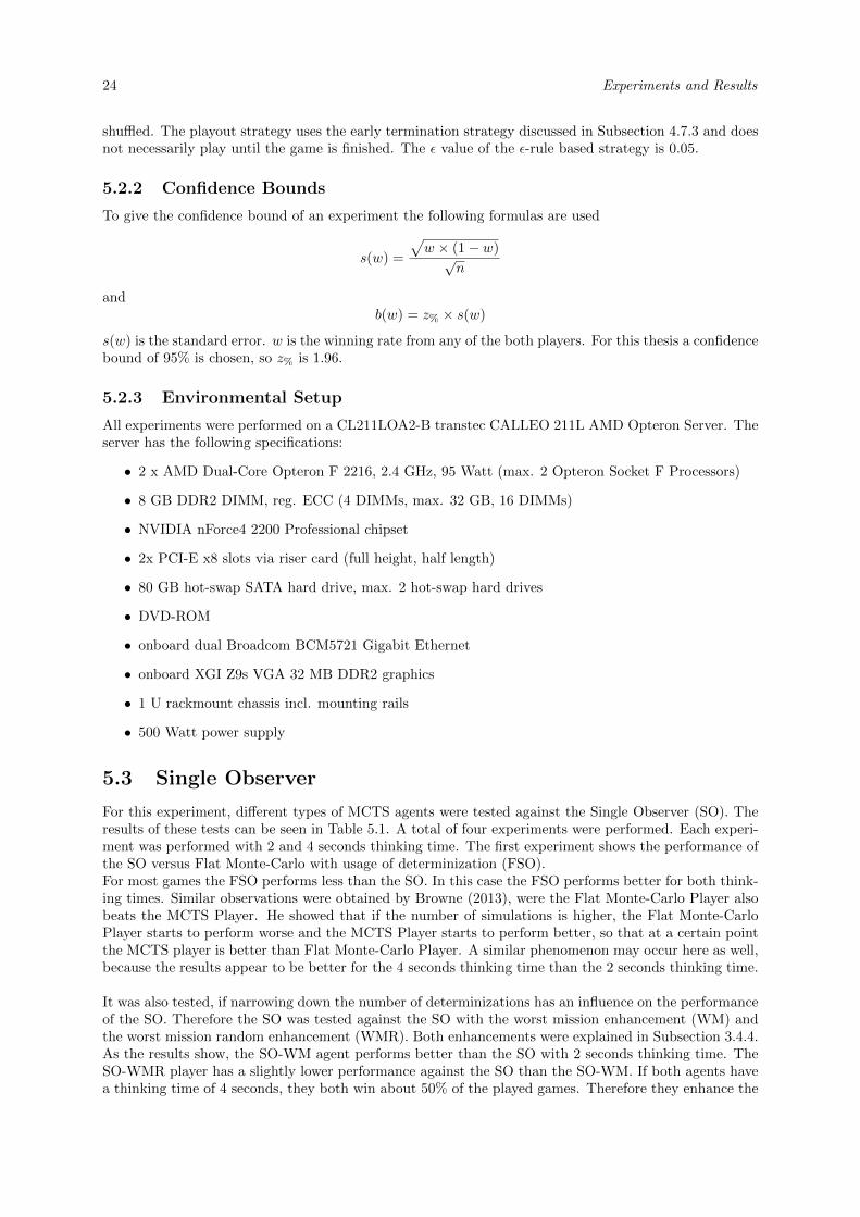
24 Experiments and Results
shuffled. The playout strategy uses the early termination strategy discussed in Subsection 4.7.3 and doesnot necessarily play until the game is finished. The ε value of the ε-rule based strategy is 0.05.
5.2.2 Confidence Bounds
To give the confidence bound of an experiment the following formulas are used
s(w) =
√w × (1− w)√
n
andb(w) = z% × s(w)
s(w) is the standard error. w is the winning rate from any of the both players. For this thesis a confidencebound of 95% is chosen, so z% is 1.96.
5.2.3 Environmental Setup
All experiments were performed on a CL211LOA2-B transtec CALLEO 211L AMD Opteron Server. Theserver has the following specifications:
• 2 x AMD Dual-Core Opteron F 2216, 2.4 GHz, 95 Watt (max. 2 Opteron Socket F Processors)
• 8 GB DDR2 DIMM, reg. ECC (4 DIMMs, max. 32 GB, 16 DIMMs)
• NVIDIA nForce4 2200 Professional chipset
• 2x PCI-E x8 slots via riser card (full height, half length)
• 80 GB hot-swap SATA hard drive, max. 2 hot-swap hard drives
• DVD-ROM
• onboard dual Broadcom BCM5721 Gigabit Ethernet
• onboard XGI Z9s VGA 32 MB DDR2 graphics
• 1 U rackmount chassis incl. mounting rails
• 500 Watt power supply
5.3 Single Observer
For this experiment, different types of MCTS agents were tested against the Single Observer (SO). Theresults of these tests can be seen in Table 5.1. A total of four experiments were performed. Each experi-ment was performed with 2 and 4 seconds thinking time. The first experiment shows the performance ofthe SO versus Flat Monte-Carlo with usage of determinization (FSO).For most games the FSO performs less than the SO. In this case the FSO performs better for both think-ing times. Similar observations were obtained by Browne (2013), were the Flat Monte-Carlo Player alsobeats the MCTS Player. He showed that if the number of simulations is higher, the Flat Monte-CarloPlayer starts to perform worse and the MCTS Player starts to perform better, so that at a certain pointthe MCTS player is better than Flat Monte-Carlo Player. A similar phenomenon may occur here as well,because the results appear to be better for the 4 seconds thinking time than the 2 seconds thinking time.
It was also tested, if narrowing down the number of determinizations has an influence on the performanceof the SO. Therefore the SO was tested against the SO with the worst mission enhancement (WM) andthe worst mission random enhancement (WMR). Both enhancements were explained in Subsection 3.4.4.As the results show, the SO-WM agent performs better than the SO with 2 seconds thinking time. TheSO-WMR player has a slightly lower performance against the SO than the SO-WM. If both agents havea thinking time of 4 seconds, they both win about 50% of the played games. Therefore they enhance the
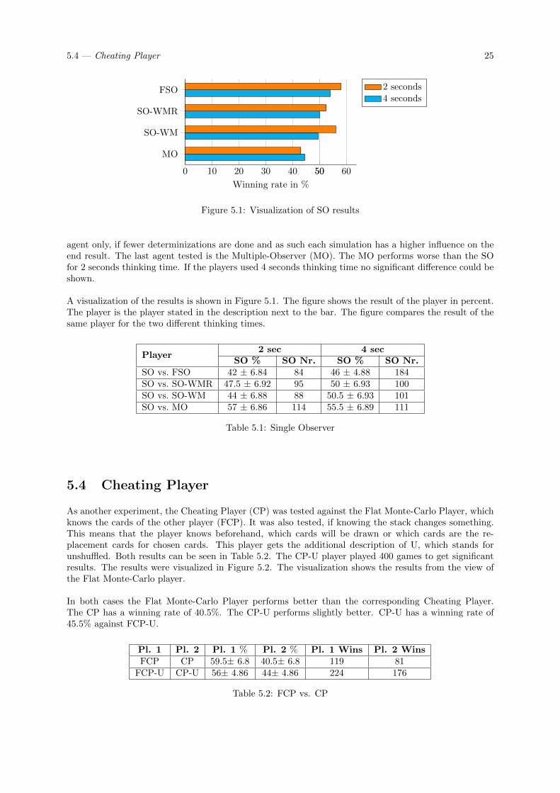
5.4 — Cheating Player 25
0 10 20 30 40 50 60
FSO
SO-WMR
SO-WM
MO
50
Winning rate in %
2 seconds4 seconds
Figure 5.1: Visualization of SO results
agent only, if fewer determinizations are done and as such each simulation has a higher influence on theend result. The last agent tested is the Multiple-Observer (MO). The MO performs worse than the SOfor 2 seconds thinking time. If the players used 4 seconds thinking time no significant difference could beshown.
A visualization of the results is shown in Figure 5.1. The figure shows the result of the player in percent.The player is the player stated in the description next to the bar. The figure compares the result of thesame player for the two different thinking times.
Player2 sec 4 sec
SO % SO Nr. SO % SO Nr.SO vs. FSO 42 ± 6.84 84 46 ± 4.88 184SO vs. SO-WMR 47.5 ± 6.92 95 50 ± 6.93 100SO vs. SO-WM 44 ± 6.88 88 50.5 ± 6.93 101SO vs. MO 57 ± 6.86 114 55.5 ± 6.89 111
Table 5.1: Single Observer
5.4 Cheating Player
As another experiment, the Cheating Player (CP) was tested against the Flat Monte-Carlo Player, whichknows the cards of the other player (FCP). It was also tested, if knowing the stack changes something.This means that the player knows beforehand, which cards will be drawn or which cards are the re-placement cards for chosen cards. This player gets the additional description of U, which stands forunshuffled. Both results can be seen in Table 5.2. The CP-U player played 400 games to get significantresults. The results were visualized in Figure 5.2. The visualization shows the results from the view ofthe Flat Monte-Carlo player.
In both cases the Flat Monte-Carlo Player performs better than the corresponding Cheating Player.The CP has a winning rate of 40.5%. The CP-U performs slightly better. CP-U has a winning rate of45.5% against FCP-U.
Pl. 1 Pl. 2 Pl. 1 % Pl. 2 % Pl. 1 Wins Pl. 2 WinsFCP CP 59.5± 6.8 40.5± 6.8 119 81
FCP-U CP-U 56± 4.86 44± 4.86 224 176
Table 5.2: FCP vs. CP

26 Experiments and Results
0 10 20 30 40 50 60
FCP
FCP-U
50
Winning rate in %
Figure 5.2: Visualization of FCP vs. CP results
0 20 40 60 80 100
SO-PU
SO-PB
SO-PUB
SO-PS
50
Winning rate in %
Figure 5.3: Visualization of FSO vs. SO with Enhancements results
5.5 Enhancements
In this section the four different enhancements are closer analyzed. They are compared to different agentsand also compared with each other.
5.5.1 FSO vs. Enhancements
The enhancements, which are tested in this section, are progressive unpruning (PU, see 3.4.1), progressivebias (PB, see 3.4.2), the combination of progressive unpruning with progressive bias (PUB) and a ε-rule based playout strategy (PS, see 4.7.3). The heuristic values, which were used for the progressiveenhancements, can be seen in Subsection 4.6.1. All enhancements were tested against the FSO first, tosee if they enhance the playout of the SO in such a way that the SO is able to defeat the FSO on average.As can be seen in Table 5.3, most enhancements, except SO-PS, are able to defeat the Flat Monte-Carloagent in more than 80% of the games. SO-PS loses over 70% of the time when playing against the FlatMonte-Carlo player. The visualization of the results, visible in Figure 5.3, shows that SO-PUB performsbest against the FSO. SO-PB wins 88.5% of all games. SO-PU performs a little bit less than the othertwo progressive approaches with winning only 87% of all games.
Pl. 1 Pl. 2 Pl. 1 % Pl. 2 % Pl. 1 Wins Pl. 2 WinsFSO SO-PU 13 ± 4.66 87 ± 4.66 26 174FSO SO-PB 11.5 ± 4.42 88.5 ± 4.42 23 177FSO SO-PUB 7.5 ± 3.65 92.5 ± 3.65 15 185FSO SO-PS 70.5 ± 6.32 40.5 ± 6.32 141 59
Table 5.3: FSO vs. SO with Enhancements
5.5.2 Improving Flat Monte-Carlo with Enhancements
To see, if the enhancements help to enhance the performance of the SO, the enhancements were testedagainst the Flat Monte-Carlo, which was also improved by the same enhancements. The results for theseexperiments can be seen in Table 5.4. The progressive approaches played 600 games in total, when theyhad 2 seconds thinking time, to get clearer results. The approaches with 2 seconds thinking time do notgive a clear result. The enhanced version of FSO seems to performs less than the enhanced SO, but theseresults are not clear. The SO-PS performs similarly to the FSO-PS with winning 49.5% of all games.To get clearer results both approaches got more thinking time, so the thinking time was increased to 4seconds.

5.5 — Enhancements 27
0 10 20 30 40 50
FSO-PU
FSO-PB
FSO-PUB
FSO-PS
50
Winning rate in %
2 seconds4 seconds
Figure 5.4: Visualization of FSO vs. SO both with enhancements
With 4 seconds thinking time the progressive unpruning approach performs best against its flat vari-ant. The other progressive variants have a slightly smaller winning rate, but both win more than 50% ofthe time. PB wins 55% of all games and PUB wins 57.5% of all games. The performance of the playoutstrategy remains the same.The visualization of the games can be seen in Figure 5.4. The results are presented in the same way asin Section 5.3.
Player2 sec 4 sec
SO % SO Nr. SO % SO Nr.SO-PU vs. FSO-PU 51 ± 4 306 60.5 ± 6.78 121SO-PB vs. FSO-PB 51.33 ± 4 308 55 ± 4.88 220SO-PUB vs. FSO-PUB 51.83 ± 4 311 57.5 ± 6.85 115SO-PS vs. FSO-PS 49.5 ± 6.32 99 48 ± 6.92 96
Table 5.4: SO vs. FSO both with Enhancements
5.5.3 SO vs. Enhancements
This section shows the results of the SO, which plays against the different enhancements. As can be seenin Table 5.5, all enhancements, except the PS, perform better than the SO without enhancements. Itwas expected that the default SO performs worse than the progressive approaches. This was expected,because the default FSO lost the majority of the games against the SO enhanced with progressive ap-proaches. However, the default FSO was able to win against the default SO more than 50% of all games.While it was expected that the heuristic enhancement performs better than the SO, it was not anticipatedthat the difference would be that significant. The worst performing enhancement, PU, wins 88% of thegames. PB wins 95% of the games and PUB even wins 99.5% of the 200 games.PS performs significantly worse than the SO with winning only 32.5% of all games.
To get a clearer overview over the results, the results were visualized in Figure 5.5. The results show theresults in percent for the enhanced players.
Pl. 1 Pl. 2 Pl. 1 % Pl. 2 % Pl. 1 Wins Pl. 2 WinsSO SO-PU 12 ± 4.5 88 ± 4.5 24 176SO SO-PB 5 ± 3.02 95 ± 3.02 10 190SO SO-PUB 0.5 ± 0.98 99.5 ± 0.98 1 199SO SO-PS 67.5 ± 6.49 32.5 ± 6.49 135 65
Table 5.5: SO vs. SO with enhancements
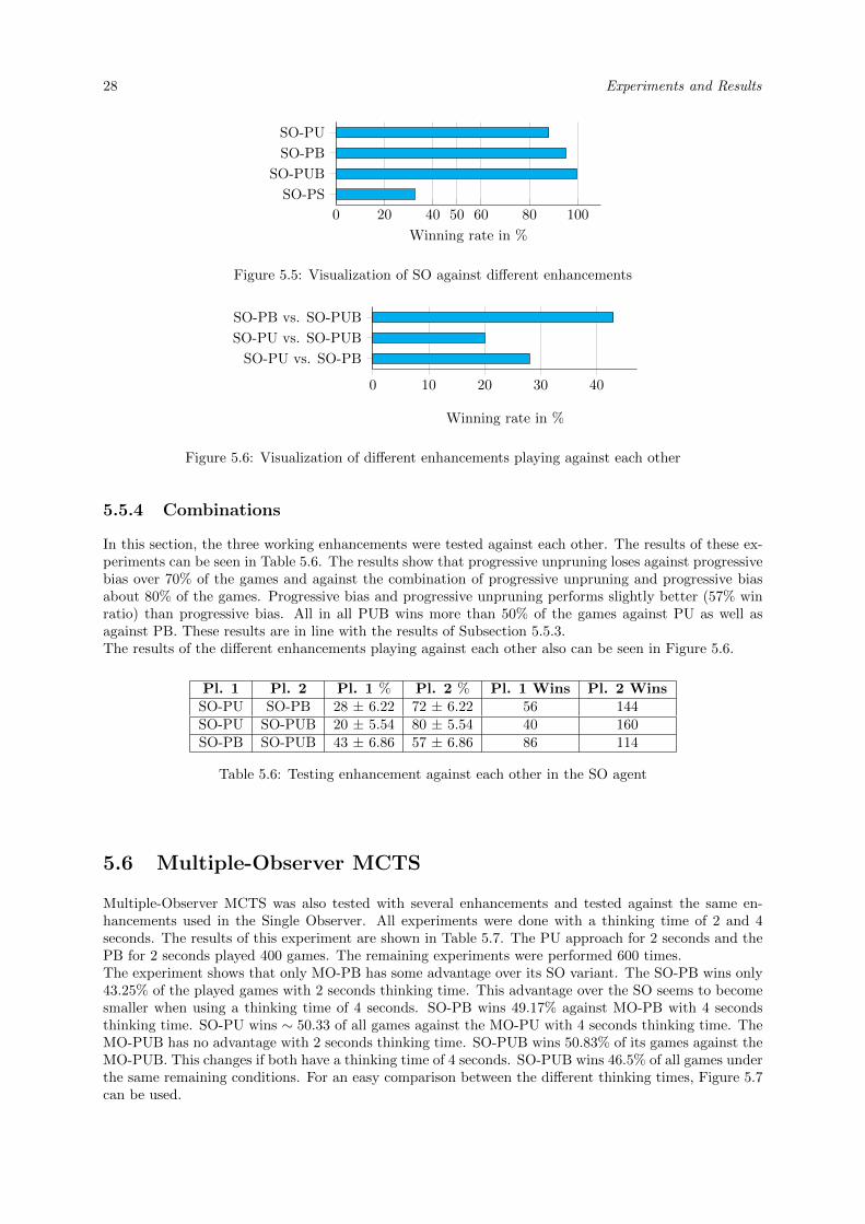
28 Experiments and Results
0 20 40 60 80 100
SO-PU
SO-PB
SO-PUB
SO-PS
50
Winning rate in %
Figure 5.5: Visualization of SO against different enhancements
0 10 20 30 40
SO-PU vs. SO-PB
SO-PU vs. SO-PUB
SO-PB vs. SO-PUB
Winning rate in %
Figure 5.6: Visualization of different enhancements playing against each other
5.5.4 Combinations
In this section, the three working enhancements were tested against each other. The results of these ex-periments can be seen in Table 5.6. The results show that progressive unpruning loses against progressivebias over 70% of the games and against the combination of progressive unpruning and progressive biasabout 80% of the games. Progressive bias and progressive unpruning performs slightly better (57% winratio) than progressive bias. All in all PUB wins more than 50% of the games against PU as well asagainst PB. These results are in line with the results of Subsection 5.5.3.The results of the different enhancements playing against each other also can be seen in Figure 5.6.
Pl. 1 Pl. 2 Pl. 1 % Pl. 2 % Pl. 1 Wins Pl. 2 WinsSO-PU SO-PB 28 ± 6.22 72 ± 6.22 56 144SO-PU SO-PUB 20 ± 5.54 80 ± 5.54 40 160SO-PB SO-PUB 43 ± 6.86 57 ± 6.86 86 114
Table 5.6: Testing enhancement against each other in the SO agent
5.6 Multiple-Observer MCTS
Multiple-Observer MCTS was also tested with several enhancements and tested against the same en-hancements used in the Single Observer. All experiments were done with a thinking time of 2 and 4seconds. The results of this experiment are shown in Table 5.7. The PU approach for 2 seconds and thePB for 2 seconds played 400 games. The remaining experiments were performed 600 times.The experiment shows that only MO-PB has some advantage over its SO variant. The SO-PB wins only43.25% of the played games with 2 seconds thinking time. This advantage over the SO seems to becomesmaller when using a thinking time of 4 seconds. SO-PB wins 49.17% against MO-PB with 4 secondsthinking time. SO-PU wins ∼ 50.33 of all games against the MO-PU with 4 seconds thinking time. TheMO-PUB has no advantage with 2 seconds thinking time. SO-PUB wins 50.83% of its games against theMO-PUB. This changes if both have a thinking time of 4 seconds. SO-PUB wins 46.5% of all games underthe same remaining conditions. For an easy comparison between the different thinking times, Figure 5.7can be used.

5.7 — Multiple Trees MCTS 29
Player2 sec 4 sec
SO % SO Nr. SO % SO Nr.SO-PU vs. MO-PU 46.75 ± 4.89 187 50.33 ± 4 302SO-PB vs. MO-PB 43.25 ± 4.86 173 49.17 ± 4 295SO-PUB vs. MO-PUB 50.83 ± 4 305 46.5 ± 3.99 279
Table 5.7: SO vs. MO both with Enhancements
0 10 20 30 40 50 60
MO-PU
MO-PB
MO-PUB
Winning rate in %
2 seconds4 seconds
Figure 5.7: Visualization of MO vs. SO both with enhancements
5.7 Multiple Trees MCTS
In this section the two different strategies, which use more than one tree to map their results, arediscussed. Both strategies were explained in Subsection 3.4.8. First both approaches are tested withoutany enhancements. Determinized UCT is then enhanced with progressive unpruning and progressive bias.Finally, the voting player is enhanced with all three progressive approaches.
5.7.1 SO vs. Determinized UCT and Voting
Determinized UCT (DZ) and voting (V) was tested with 1, 5, 10 and 20 trees and played against the SOwith the same enhancements. It has to be considered that both approaches when they are using only onetree are the same. This also means that for each tree only a certain randomly calculated determinizationwas chosen. Determinized UCT with 1 and 10 trees played 400 games instead of the usual 200 games.The results can be seen in Table 5.8 and Figure 5.8.The results show that the SO performs clearly better than all voting agents. The determinized UCT alsoseems to perform better than the voting player, but in most cases this improvement is rather small. Theonly approach, where the voting player performed better than the determinized UCT against the SO wasfor 20 trees. The voting player was able to win 41.5% of all games, while the determinized UCT playerwas only able to win 38.5% of all games. The determinized UCT player was also not able to performsignificantly better than the SO. Determinized UCT performs best with using only one tree, in whichcase no player performs significantly better than the other one.
PlayerDeterminized UCT Voting
SO % SO Nr. SO % SO Nr.SO vs. 1 Tree 50.75 ± 4.9 203 58 ± 6.84 116SO vs. 5 Trees 57.5 ± 6.85 115 58.5 ± 6.83 117SO vs. 10 Trees 56.25 ± 4.86 225 62.5 ± 6.71 125SO vs. 20 Trees 61.5 ± 6.74 123 58.5 ± 6.83 117
Table 5.8: SO vs. Determinized UCT and Voting
5.7.2 Determinized UCT
In this subsection, determinized UCT is closer analyzed. The enhancements, which were tested, areprogressive unpruning or progressive bias. The results are shown in Table 5.9.The results show, that SO-PB performs clearly better than all DZ players. These results can be compared
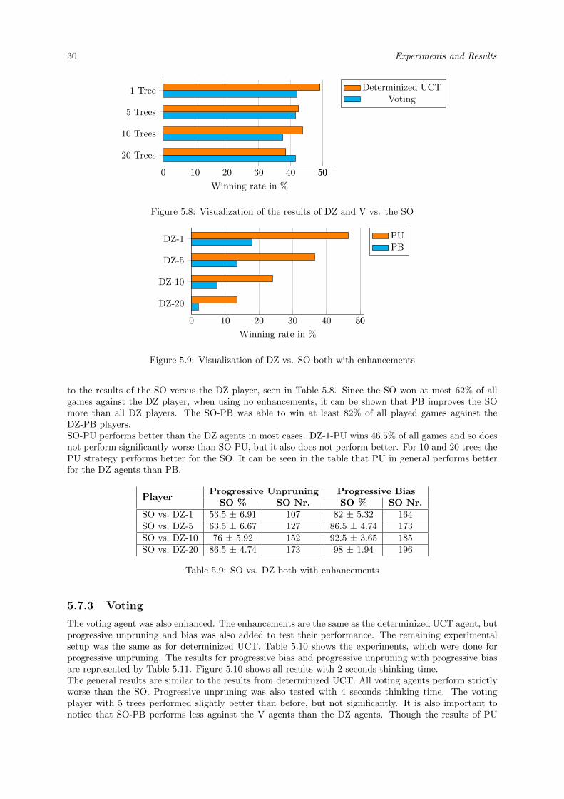
30 Experiments and Results
0 10 20 30 40 50
1 Tree
5 Trees
10 Trees
20 Trees
50
Winning rate in %
Determinized UCTVoting
Figure 5.8: Visualization of the results of DZ and V vs. the SO
0 10 20 30 40 50
DZ-1
DZ-5
DZ-10
DZ-20
50
Winning rate in %
PUPB
Figure 5.9: Visualization of DZ vs. SO both with enhancements
to the results of the SO versus the DZ player, seen in Table 5.8. Since the SO won at most 62% of allgames against the DZ player, when using no enhancements, it can be shown that PB improves the SOmore than all DZ players. The SO-PB was able to win at least 82% of all played games against theDZ-PB players.SO-PU performs better than the DZ agents in most cases. DZ-1-PU wins 46.5% of all games and so doesnot perform significantly worse than SO-PU, but it also does not perform better. For 10 and 20 trees thePU strategy performs better for the SO. It can be seen in the table that PU in general performs betterfor the DZ agents than PB.
PlayerProgressive Unpruning Progressive Bias
SO % SO Nr. SO % SO Nr.SO vs. DZ-1 53.5 ± 6.91 107 82 ± 5.32 164SO vs. DZ-5 63.5 ± 6.67 127 86.5 ± 4.74 173SO vs. DZ-10 76 ± 5.92 152 92.5 ± 3.65 185SO vs. DZ-20 86.5 ± 4.74 173 98 ± 1.94 196
Table 5.9: SO vs. DZ both with enhancements
5.7.3 Voting
The voting agent was also enhanced. The enhancements are the same as the determinized UCT agent, butprogressive unpruning and bias was also added to test their performance. The remaining experimentalsetup was the same as for determinized UCT. Table 5.10 shows the experiments, which were done forprogressive unpruning. The results for progressive bias and progressive unpruning with progressive biasare represented by Table 5.11. Figure 5.10 shows all results with 2 seconds thinking time.The general results are similar to the results from determinized UCT. All voting agents perform strictlyworse than the SO. Progressive unpruning was also tested with 4 seconds thinking time. The votingplayer with 5 trees performed slightly better than before, but not significantly. It is also important tonotice that SO-PB performs less against the V agents than the DZ agents. Though the results of PU
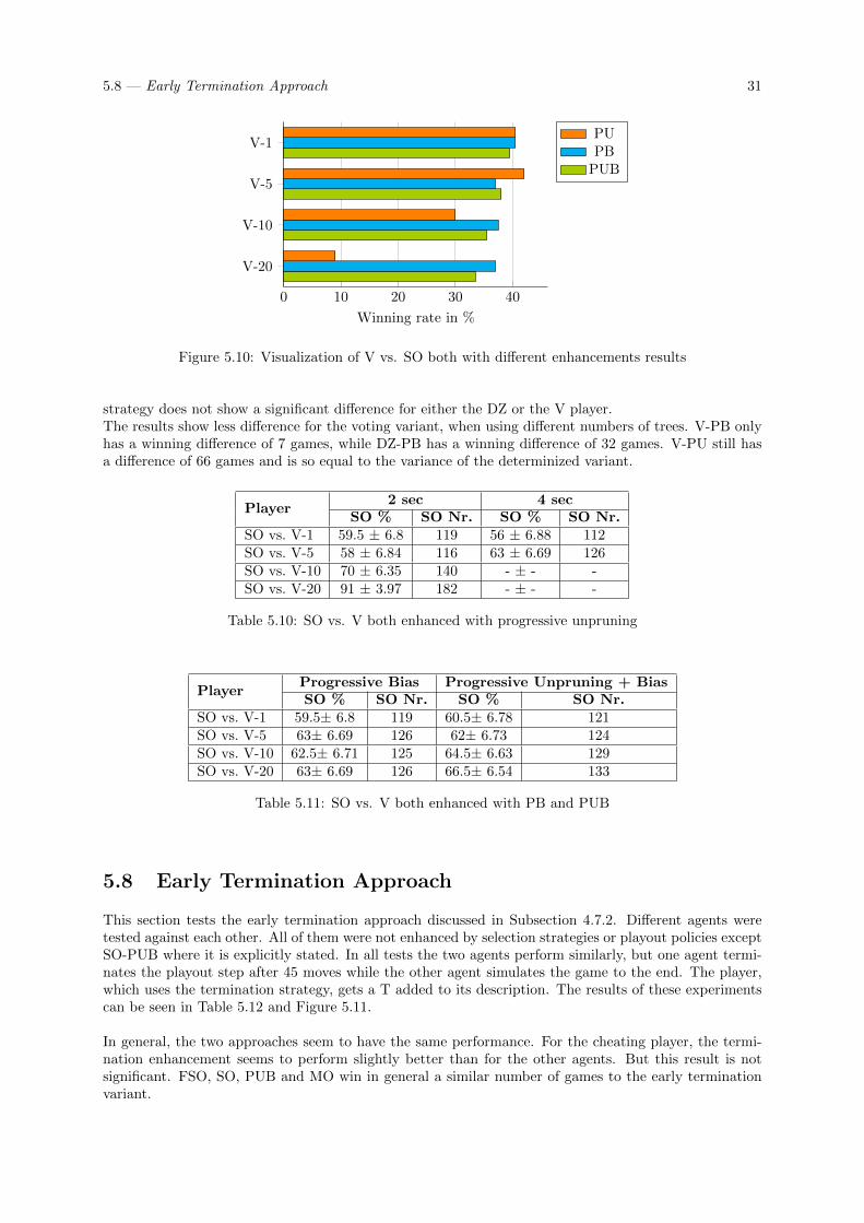
5.8 — Early Termination Approach 31
0 10 20 30 40
V-1
V-5
V-10
V-20
Winning rate in %
PUPB
PUB
Figure 5.10: Visualization of V vs. SO both with different enhancements results
strategy does not show a significant difference for either the DZ or the V player.The results show less difference for the voting variant, when using different numbers of trees. V-PB onlyhas a winning difference of 7 games, while DZ-PB has a winning difference of 32 games. V-PU still hasa difference of 66 games and is so equal to the variance of the determinized variant.
Player2 sec 4 sec
SO % SO Nr. SO % SO Nr.SO vs. V-1 59.5 ± 6.8 119 56 ± 6.88 112SO vs. V-5 58 ± 6.84 116 63 ± 6.69 126SO vs. V-10 70 ± 6.35 140 - ± - -SO vs. V-20 91 ± 3.97 182 - ± - -
Table 5.10: SO vs. V both enhanced with progressive unpruning
PlayerProgressive Bias Progressive Unpruning + BiasSO % SO Nr. SO % SO Nr.
SO vs. V-1 59.5± 6.8 119 60.5± 6.78 121SO vs. V-5 63± 6.69 126 62± 6.73 124SO vs. V-10 62.5± 6.71 125 64.5± 6.63 129SO vs. V-20 63± 6.69 126 66.5± 6.54 133
Table 5.11: SO vs. V both enhanced with PB and PUB
5.8 Early Termination Approach
This section tests the early termination approach discussed in Subsection 4.7.2. Different agents weretested against each other. All of them were not enhanced by selection strategies or playout policies exceptSO-PUB where it is explicitly stated. In all tests the two agents perform similarly, but one agent termi-nates the playout step after 45 moves while the other agent simulates the game to the end. The player,which uses the termination strategy, gets a T added to its description. The results of these experimentscan be seen in Table 5.12 and Figure 5.11.
In general, the two approaches seem to have the same performance. For the cheating player, the termi-nation enhancement seems to perform slightly better than for the other agents. But this result is notsignificant. FSO, SO, PUB and MO win in general a similar number of games to the early terminationvariant.
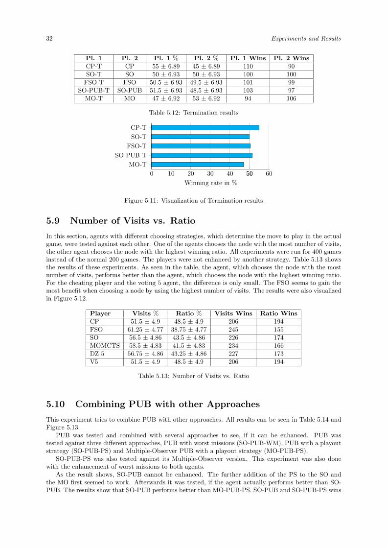
32 Experiments and Results
Pl. 1 Pl. 2 Pl. 1 % Pl. 2 % Pl. 1 Wins Pl. 2 WinsCP-T CP 55 ± 6.89 45 ± 6.89 110 90SO-T SO 50 ± 6.93 50 ± 6.93 100 100
FSO-T FSO 50.5 ± 6.93 49.5 ± 6.93 101 99SO-PUB-T SO-PUB 51.5 ± 6.93 48.5 ± 6.93 103 97
MO-T MO 47 ± 6.92 53 ± 6.92 94 106
Table 5.12: Termination results
0 10 20 30 40 50 60
CP-T
SO-T
FSO-T
SO-PUB-T
MO-T
50
Winning rate in %
Figure 5.11: Visualization of Termination results
5.9 Number of Visits vs. Ratio
In this section, agents with different choosing strategies, which determine the move to play in the actualgame, were tested against each other. One of the agents chooses the node with the most number of visits,the other agent chooses the node with the highest winning ratio. All experiments were run for 400 gamesinstead of the normal 200 games. The players were not enhanced by another strategy. Table 5.13 showsthe results of these experiments. As seen in the table, the agent, which chooses the node with the mostnumber of visits, performs better than the agent, which chooses the node with the highest winning ratio.For the cheating player and the voting 5 agent, the difference is only small. The FSO seems to gain themost benefit when choosing a node by using the highest number of visits. The results were also visualizedin Figure 5.12.
Player Visits % Ratio % Visits Wins Ratio WinsCP 51.5 ± 4.9 48.5 ± 4.9 206 194FSO 61.25 ± 4.77 38.75 ± 4.77 245 155SO 56.5 ± 4.86 43.5 ± 4.86 226 174MOMCTS 58.5 ± 4.83 41.5 ± 4.83 234 166DZ 5 56.75 ± 4.86 43.25 ± 4.86 227 173V5 51.5 ± 4.9 48.5 ± 4.9 206 194
Table 5.13: Number of Visits vs. Ratio
5.10 Combining PUB with other Approaches
This experiment tries to combine PUB with other approaches. All results can be seen in Table 5.14 andFigure 5.13.
PUB was tested and combined with several approaches to see, if it can be enhanced. PUB wastested against three different approaches, PUB with worst missions (SO-PUB-WM), PUB with a playoutstrategy (SO-PUB-PS) and Multiple-Observer PUB with a playout strategy (MO-PUB-PS).
SO-PUB-PS was also tested against its Multiple-Observer version. This experiment was also donewith the enhancement of worst missions to both agents.
As the result shows, SO-PUB cannot be enhanced. The further addition of the PS to the SO andthe MO first seemed to work. Afterwards it was tested, if the agent actually performs better than SO-PUB. The results show that SO-PUB performs better than MO-PUB-PS. SO-PUB and SO-PUB-PS wins
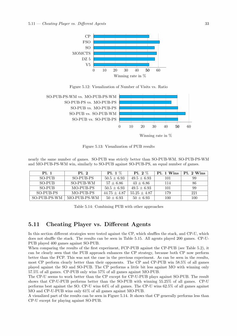
5.11 — Cheating Player vs. Different Agents 33
0 10 20 30 40 50 60
CP
FSO
SO
MOMCTS
DZ 5
V5
50
Winning rate in %
Figure 5.12: Visualization of Number of Visits vs. Ratio
0 10 20 30 40 50 60
SO-PUB vs. SO-PUB-PS
SO-PUB vs. SO-PUB-WM
SO-PUB vs. MO-PUB-PS
SO-PUB-PS vs. MO-PUB-PS
SO-PUB-PS-WM vs. MO-PUB-PS-WM
50
Winning rate in %
Figure 5.13: Visualization of PUB results
nearly the same number of games. SO-PUB was strictly better than SO-PUB-WM. SO-PUB-PS-WMand MO-PUB-PS-WM win, similarly to SO-PUB against SO-PUB-PS, an equal number of games.
Pl. 1 Pl. 2 Pl. 1 % Pl. 2 % Pl. 1 Wins Pl. 2 WinsSO-PUB SO-PUB-PS 50.5 ± 6.93 49.5 ± 6.93 101 99SO-PUB SO-PUB-WM 57 ± 6.86 43 ± 6.86 114 86SO-PUB MO-PUB-PS 50.5 ± 6.93 49.5 ± 6.93 101 99
SO-PUB-PS MO-PUB-PS 44.75 ± 4.87 55.25 ± 4.87 179 221SO-PUB-PS-WM MO-PUB-PS-WM 50 ± 6.93 50 ± 6.93 100 100
Table 5.14: Combining PUB with other approaches
5.11 Cheating Player vs. Different Agents
In this section different strategies were tested against the CP, which shuffles the stack, and CP-U, whichdoes not shuffle the stack. The results can be seen in Table 5.15. All agents played 200 games. CP-U-PUB played 400 games against SO-PUB.When comparing the results of the first experiment, FCP-PUB against the CP-PUB (see Table 5.2), itcan be clearly seen that the PUB approach enhances the CP strategy, because both CP now performbetter than the FCP. This was not the case in the previous experiment. As can be seen in the results,most CP perform clearly better than their opponents. The CP and CP-PUB win 58.5% of all gamesplayed against the SO and SO-PUB. The CP performs a little bit less against MO with winning only57.5% of all games. CP-PUB only wins 57% of all games against MO-PUB.The CP-U seems to work better than the CP except for CP-U-PUB plays against SO-PUB. The resultshows that CP-U-PUB performs better than the SO-PUB with winning 55.25% of all games. CP-Uperforms best against the SO. CP-U wins 64% of all games. The CP-U wins 62.5% of all games againstMO and CP-U-PUB wins only 61% of all games against MO-PUB.A visualized part of the results can be seen in Figure 5.14. It shows that CP generally performs less thanCP-U except for playing against SO-PUB.

34 Experiments and Results
PlayerCP Shuffled CP Fixed (CP-U)
CP % CP Nr. CP % CP Nr.CP-PUB vs. FCP-PUB 59.5 ± 6.8 119 61.5 ± 6.74 123CP vs. SO 58.5 ± 6.83 117 64 ± 6.65 128CP-PUB vs. SO-PUB 58.5 ± 6.83 117 55.25 ± 3.45 442CP vs. MO 57.5 ± 6.85 115 62.5 ± 6.71 125CP-PUB vs. MO-PUB 57 ± 6.86 114 61 ± 6.76 122
Table 5.15: CP vs. different agents
0 10 20 30 40
FCP-PUB
SO
SO-PUB
MO
MO-PUB
Winning rate in %
CPCP-U
Figure 5.14: Visualization of CP vs. different agents
5.12 Completing destination tickets
During the experiments it became apparent that unimproved strategies like the SO were not able tocomplete destination tickets. In a normal two player game, both players should be able to fulfill at leasttwo destination tickets most of the time.
As an example, when the FSO played against the SO with 2 seconds thinking time, the FSO was ableto complete 0.5 destination tickets while the SO was able to complete 0.51 destination tickets on average.The average number of victory points for both players is 42.07. This is not a good result for any Ticketto Ride player. These results could be explained with too few simulations and the too complex structureof Ticket to Ride. Especially the first destination tickets take the longest time to complete.
As another example, when the FSO-PUB played against the SO-PUB with 2 seconds thinking time, theFSO-PUB was able to complete 3.83 destination tickets on average. The SO-PUB was able to complete4.11 destination tickets. This suggests that the enhancements actually guide the MCTS algorithm tocompleting more missions. This results also in more points. Both players are able to score 96.58 victorypoints. The victory points of the unimproved FSO and SO are therefore more than doubled.
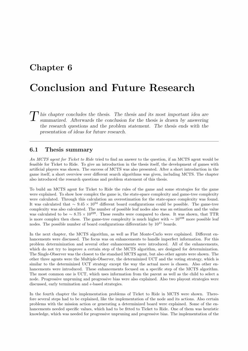
Chapter 6
Conclusion and Future Research
T his chapter concludes the thesis. The thesis and its most important idea aresummarized. Afterwards the conclusion for the thesis is drawn by answeringthe research questions and the problem statement. The thesis ends with thepresentation of ideas for future research.
6.1 Thesis summary
An MCTS agent for Ticket to Ride tried to find an answer to the question, if an MCTS agent would befeasible for Ticket to Ride. To give an introduction in the thesis itself, the development of games withartificial players was shown. The success of MCTS was also presented. After a short introduction in thegame itself, a short overview over different search algorithms was given, including MCTS. The chapteralso introduced the research questions and problem statement of this thesis.
To build an MCTS agent for Ticket to Ride the rules of the game and some strategies for the gamewere explained. To show how complex the game is, the state-space complexity and game-tree complexitywere calculated. Through this calculation an overestimation for the state-space complexity was found.It was calculated that ∼ 9.45 × 1054 different board configurations could be possible. The game-treecomplexity was also calculated. The number of possible leaf nodes also was an estimation and the valuewas calculated to be ∼ 8.75 × 10228. These results were compared to chess. It was shown, that TTRis more complex then chess. The game-tree complexity is much higher with ∼ 10108 more possible leafnodes. The possible number of board configurations differentiate by 1011 boards.
In the next chapter, the MCTS algorithm, as well as Flat Monte-Carlo were explained. Different en-hancements were discussed. The focus was on enhancements to handle imperfect information. For thisproblem determinization and several other enhancements were introduced. All of the enhancements,which do not try to improve a certain step of the MCTS algorithm, are designed for determinization.The Single-Observer was the closest to the standard MCTS agent, but also other agents were shown. Theother three agents were the Multiple-Observer, the determinized UCT and the voting strategy, which issimilar to the determinized UCT strategy except the way the actual move is chosen. Also other en-hancements were introduced. These enhancements focused on a specific step of the MCTS algorithm.The most common one is UCT, which uses information from the parent as well as the child to select anode. Progressive unpruning and progressive bias were also explained. Also two playout strategies werediscussed, early termination and ε-based strategies.
In the fourth chapter the implementation problems of Ticket to Ride in MCTS were shown. There-fore several steps had to be explained, like the implementation of the node and its actions. Also certainproblems with the mission action or generating a determinized board were explained. Some of the en-hancements needed specific values, which had to be fitted to Ticket to Ride. One of them was heuristicknowledge, which was needed for progressive unpruning and progressive bias. The implementation of the
36 Conclusion and Future Research
playout strategy also needed a more detailed explanation.
In the fifth chapter, the introduced players and enhancements were tested. Therefore the setup of theexperiments was described. All values from certain constants of different players, were stated as well.Afterwards different experiments were performed and evaluated.
The experiment showed, that MCTS was not necessarily working better than Flat Monte-Carlo. Inmost cases the addition of the tree could enhance a player. Therefore it was decided to enhance bothplayers even further. The addition of progressive unpruning, progressive bias or a combination of both,seemed to make both players at least equal. The Single-Observer with one of the progressive enhance-ments seemed to work better than its Flat Monte-Carlo variant when having a thinking time of 4 seconds.
Through the experiments it can be concluded as well that several approaches like the voting player or thedeterminized UCT player do not work when they are enhanced with one of the progressive approaches.Multiple-Observer seemed to work for progressive bias and progressive unpruning with 2 second thinkingtime. Otherwise it did not seem to make a difference except for the combination of both progressiveapproaches, which worked better, when it had 4 seconds thinking time.
It was also tested, if the actual selection of the move would be better, if the node with the highestwinning ratio would be chosen. It was shown that most players could not be improved with this choosingstrategy. For the cheating player and the voting 5 player it is not proven that one strategy is better thanthe other one. At the moment it seems that neither strategy improves the cheating nor the voting 5 player.
The early termination could only bring a small enhancement to the cheating player. Otherwise thetermination approach did not work better for most approaches except Multiple-Observer, which per-formed worse. Overall it was found that progressive unpruning combined with progressive bias workedbest, so it was tested combined with several other approaches. In the end, it was not clear if progressiveunpruning combined only with progressive bias works best, but other different enhancements with whichit was tested, did not give a boost in performance or made the agent perform worse.
The two approaches to choose missions during the determinization seemed to work better for 2 sec-onds thinking time. When changing the thinking time to 4 seconds both agents performed as well as theSingle-Observer. It was tried to add the better working approach to the combination of progressive un-pruning combined with progressive bias. This approach was the one who chooses the destination ticketssuch that it would be worse for the momentarily active player. This player was tested against the sameplayer without the worst missions enhancement. The more enhanced player performed significantly worse.
The cheating player was the last player, which was tested. The cheating player was tested in twodifferent ways. One player knew the stack the other one did not. Both agents performed better thanthe Single-Observer and the Multiple-Observer they were tested against. But a unexpected result wasobtained when both agents were enhanced with the combination of the progressive approaches. There theplayer which knew the stack, did not have a necessarily better performance against the Single-Observer.Both types of cheating players were tested against the Flat Monte-Carlo player. Both were not able todefeat the Flat Monte-Carlo more than 56% percent of the time, which is unusual. If both strategieswere enhanced with the combination of progressive unpruning and progressive bias, the cheating playerwas able to defeat the flat cheating player about 59.5% of all games.
6.2 Answering the Research Questions
The research questions were given in Section 1.3. These questions are answered first, before an answerto the problem statement is given.
Are Monte-Carlo methods applicable to Ticket to Ride?Monte-Carlo methods seem to work in Ticket to Ride. Without any enhancement the Flat Monte-Carloseemed to work best for a thinking time of 2 seconds. If the player should not cheat, determinization had
6.3 — Answering the Problem Statement 37
to be implemented such that the implemented player would have the same preconditions as a humanoidplayer.
How can MCTS handle the imperfect-information game in the domain of TTR?To test how well MCTS handles imperfect information several strategies were tested against the cheatingMCTS player. The Single- and Multiple-Observer perform worse than the cheating player. This resultwas expected, because the cheating player knows the cards of his opponent and can block the player.The Single-Observer and Multiple-Observer win 42% of all games against the cheating player, which isshuffled. The Single-Observer and Multiple Observer performed worse against the cheating player withnon-shuffled stacks by winning only 39% of all played games. Considering the disadvantage of the Single-Observer and Multiple-Observer, they still perform well against both types of cheating player.
Which enhancements can improve the MCTS player?As discussed before, progressive bias, progressive unpruning and the combination of both can enhanceMCTS. The Multiple-Observer enhances MCTS only under certain conditions. The playout strategy wasnot able to enhance the MCTS player. Terminating the playout early as well as using the voting ordeterminized UCT player, do not enhance the MCTS player.
6.3 Answering the Problem Statement
This section will answer the following question, which was first introduced in Section 1.3:
How can a MCTS player for TTR be developed?
Developing an MCTS player for Ticket to Ride was not as easy as it first may have seemed to be.Several facts and conditions have to be kept in mind. One of the bigger problems was that Ticket toRide has hidden information and chance events. Therefore determinization has to be used, so MCTShas the same conditions as a human. Determinization had several problems of its own, which neededfurther investigation. Therefore several other strategies had to be closer analyzed, like the Single- andMultiple-Observer. Through the high variety of possible missions and the game length, MCTS seemednot to be able to fulfill missions on its own. Several approaches were tested improve the performance. Thecombination of progressive unpruning and progressive bias seems to work the best. A further improve-ment of this approach could not be shown in this thesis. The best player seems to be progressive biascombined with progressive unpruning either for the Single-Observer or the Multiple-Observer. NeitherSingle-Observer nor Multiple-Observer seems to perform better than the other when enhanced with theprogressive combination. To enhance the best player even more seemed to be difficult, because the moreenhanced player either performed worse or there was no significant difference.
6.4 Future Research
This section describes ideas for future research. Several strategies use constants. These constants canbe tweaked, as discussed in the corresponding parts. The C value of UCT is used in most strategiesand therefore would be a good choice. Progressive unpruning, progressive bias and the combination ofboth could also be an interesting choice to tune the parameters, because progressive bias combined withprogressive unpruning is the best strategy and could maybe be enhanced by testing different values forthe T constant. The values for A and B from the progressive unpruning could also be a good choice.Tuning the ε parameter of the rule-based strategy could maybe increase the performance. Testing moretrees for determinized UCT and the voting strategy does not seem to be plausible, because it seemed toperform worse the more trees were used.
The second idea for future research possibilities could be to test the game with three players or more. Intheory the game can be played with up to five players. This thesis covers only the two player variant. Itis important to notice that with more than three players, the game rules slightly change because moretracks become available. In general, the game with more than two players is more difficult, because it isharder to analyze in advance. Especially getting cards can become more difficult, since several players
38 Conclusion and Future Research
may need the same color. It also gets more likely that at least two players need to build the same track.Therefore multiple tracks were introduced when playing with more than three players.
Similar to the idea of playing the game with more than two players, would be to test the strategieswith different expansions or stand-alone editions. Most expansions can only be played on a certainboard, so they add most of the time only one or two rules. This changes the strategies a human playerwould use and it would be interesting to see, if MCTS is able to adapt to this change of ruling and is ableto perform similarly. An interesting edition could be the Europe variant, where a player is able to usetracks of other players then placing certain pieces on the map. Another expansion, which was designedfor two or three players, was the Netherlands expansion. It also uses double tracks, but players can buildon both of them, even with only two or three players instead of the normal four or five players.
Another possibility would be, to test the strategies against different human players to see if the strate-gies also work against them. Until now it was only tested against Monte-Carlo players and it would beinteresting to know, if MCTS is able to win against a human player.
The last idea would be to change the selection of the first destination tickets. The tickets could alsobe chosen with domain knowledge. Therefore a test of all different combinations of destination tickets isnecessary. Each pair of destination tickets would be tested against different other combinations multipletimes. For each test, the combination of the beginning tickets and the end score of the player has to besaved. This knowledge would be used to choose the two tickets with the highest total score.
References
Allis, L. V. (1994). Searching for Solutions in Games and Artificial Intelligence. Ph.D. thesis, Universityof Limburg, Maastricht, The Netherlands. [8]
Brugmann, B. (1993). Monte Carlo Go. Technical report, Physics Department, Syracuse University. [1,11]
Browne, C. (2013). A Problem Case for UCT. Computational Intelligence and AI in Games, IEEETransactions on, Vol. 5, No. 1, pp. 69–74. [24]
Browne, C., Powley, E. J., Whitehouse, D., Lucas, S. M., Cowling, P. I., Rohlfshagen, P., Tavener, S.,Perez, D., Samothrakis, S., and Colton, S. (2012). A Survey of Monte Carlo Tree Search Methods.IEEE Trans. Comput. Intellig. and AI in Games, Vol. 4, No. 1, pp. 1–43. [3]
Buro, M., Long, J. R., Furtak, T., and Sturtevant, N. R. (2009). Improving State Evaluation, Inference,and Search in Trick-Based Card Games. IJCAI (ed. C. Boutilier), pp. 1407–1413. [13]
Campbell, M., Hoane Jr., A. J., and Hsu, F.-h. (2002). Deep Blue. Artificial Intelligence, Vol. 134, Nos.1–2, pp. 57–83. [1]
Cazenave, T. (2006). A Phantom-Go Program. Advances in Computer Games (eds. H. J. van den Herik,S.-C. Hsu, T.-S. Hsu, and H. H. L. M. J. Donkers), Vol. 4250 of Lecture Notes in Computer Science,pp. 120–125. Springer Berlin Heidelberg. [13]
Chaslot, G. M. J.-B., Winands, M. H. M., van den Herik, H. J., Uiterwijk, J. W. H. M., and Bouzy,B. (2008). Progressive Strategies for Monte-Carlo Tree Search. New Mathematics and NaturalComputation, Vol. 4, pp. 343–357. [3, 12, 13]
Coulom, R. (2007a). Efficient Selectivity and Backup Operators in Monte-Carlo Tree Search. Computersand Games (eds. H. J. van den Herik, P. Ciancarini, and H. H. L. M. J. Donkers), Vol. 4630 ofLecture Notes in Computer Science, pp. 72–83. Springer Berlin Heidelberg. [1, 2, 11]
Coulom, R. (2007b). Computing “Elo Ratings” of Move Patterns in the Game of Go. ICGA Journal,Vol. 30, No. 4, pp. 198–208. [3, 12]
Cowling, P. I., Powley, E. J., and Whitehouse, D. (2012). Information Set Monte Carlo Tree Search.IEEE Trans. Comput. Intellig. and AI in Games, Vol. 4, No. 2, pp. 120–143. [2, 3, 13, 14, 15]
Dijkstra, E. W. (1959). A Note on Two Problems in Connexion with Graphs. Numerische Mathematik1, Vol. 1, No. 1, pp. 269–271. [2]
Douglas, J. R. (1978). Chess 4.7 Versus David Levy. Byte Magazine, Vol. 3, No. 12, pp. 86–93. [1]
Fern, A. and Lewis, P. (2011). Ensemble Monte-Carlo Planning: An Empirical Study. ICAPS (eds. F.Bacchus, C. Domshlak, S. Edelkamp, and M. Helmert), AAAI. [15]
Frank, I. and Basin, D. A. (1998). Search in Games with Incomplete Information: A Case Study UsingBridge Card Play. Artificial Intelligence, Vol. 100, Nos. 1–2, pp. 87–123. [13]
Ginsberg, M. L. (1999). GIB: Steps Toward an Expert-Level Bridge-Playing Program. In Proceedings ofthe Sixteenth International Joint Conference on Artificial Intelligence (IJCAI-99, pp. 584–589. [13]
40 References
Ginsberg, M. L. (2001). GIB: Imperfect Information in a Computationally Challenging Game. J. Artif.Intell. Res. (JAIR), Vol. 14, pp. 303–358. [2]
Hart, P. E., Nilsson, N. J., and Raphael, B. (1968). A Formal Basis for the Heuristic Determination ofMinimum Cost Paths. Systems Science and Cybernetics, Vol. 4, No. 2, pp. 100–107. [2]
Knuth, D. E. and Moore, R. W. (1975). An Analysis of Alpha–Beta Pruning. Artificial Intelligence,Vol. 6, No. 4, pp. 293–326. [2]
Kocsis, L. and Szepesvari, C. (2006). Bandit Based Monte-Carlo Planning. Machine Learning: ECML2006 (eds. J. Furnkranz, T. Scheffer, and M. Spiliopoulou), Vol. 4212 of Lecture Notes in ComputerScience, pp. 282–293. Springer Berlin Heidelberg. [1, 11, 12]
Lorentz, R. J. (2008). Amazons Discover Monte-Carlo. Computers and Games (eds. H. J. van den Herik,X. Xu, Z. Ma, and M. H. M. Winands), Vol. 5131 of Lecture Notes in Computer Science, pp. 13–24.Springer Berlin Heidelberg. [3, 15]
Luckhart, C. and Irani, K. B. (1986). An Algorithmic Solution of N-Person Games. AAAI, pp. 158–162,Morgan Kaufmann. [2]
Michie, D. (1966). Game-playing and Game-learning Automata. Advances in Programming and Non-Numerical Computation, Leslie Fox, Vol. 47, No. 7, pp. 183–200. [2]
Moon, A. R. (2015). Ticket to Ride. http://cdn1.daysofwonder.com/tickettoride/en/img/tt_
rules_2013_en.pdf. [Online; accessed 22.02.2015]. [7]
Nijssen, P. and Winands, M. H. M. (2012). Monte Carlo Tree Search for the Hide-and-Seek GameScotland Yard. Computational Intelligence and AI in Games, IEEE Transactions on, Vol. 4, No. 4,pp. 282–294. [3, 15]
Shannon, C. E. (1950). XXII. Programming a Computer for Playing Chess. Philosophical Magazine(Series 7), Vol. 41, No. 314, pp. 256–275. [9]
Szita, I., Chaslot, G., and Spronck, P. (2010). Monte-Carlo Tree Search in Settlers of Catan. Advances inComputer Games (eds. H. J. van den Herik and P. Spronck), Vol. 6048 of Lecture Notes in ComputerScience, pp. 21–32. Springer Berlin Heidelberg. [2]
Von Neumann, J. and Morgenstern, O. (1944). Theory of Games and Economic Behavior. PrincetonUniversity Press. [2]
Wedd, N. (2015). Human-Computer Go Challenges. http://www.computer-go.info/h-c/. [Online;accessed 09.02.2015]. [1]
Winands, M. H. M. and Bjornsson, Y. (2010). Evaluation Function Based Monte-Carlo LOA. Advances inComputer Games (eds. H. J. van den Herik and P. Spronck), Vol. 6048 of Lecture Notes in ComputerScience, pp. 33–44. Springer Berlin Heidelberg. [15]
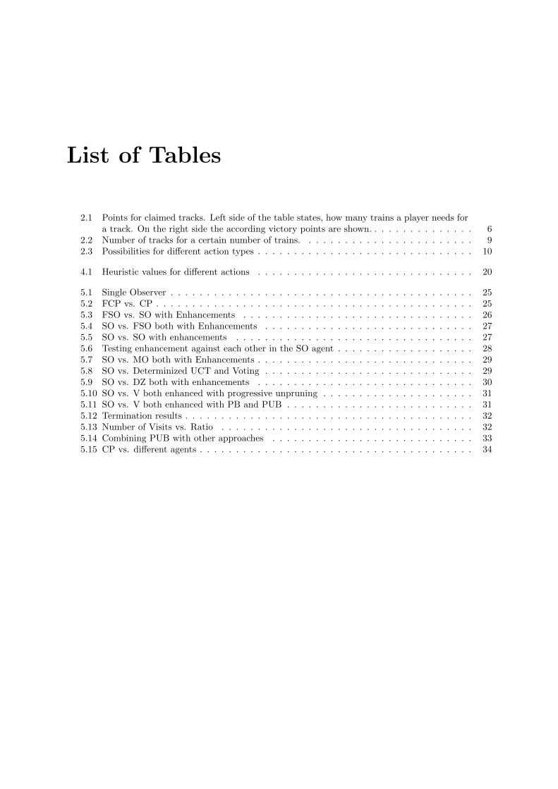
List of Tables
2.1 Points for claimed tracks. Left side of the table states, how many trains a player needs fora track. On the right side the according victory points are shown. . . . . . . . . . . . . . . 6
2.2 Number of tracks for a certain number of trains. . . . . . . . . . . . . . . . . . . . . . . . 92.3 Possibilities for different action types . . . . . . . . . . . . . . . . . . . . . . . . . . . . . . 10
4.1 Heuristic values for different actions . . . . . . . . . . . . . . . . . . . . . . . . . . . . . . 20
5.1 Single Observer . . . . . . . . . . . . . . . . . . . . . . . . . . . . . . . . . . . . . . . . . . 255.2 FCP vs. CP . . . . . . . . . . . . . . . . . . . . . . . . . . . . . . . . . . . . . . . . . . . . 255.3 FSO vs. SO with Enhancements . . . . . . . . . . . . . . . . . . . . . . . . . . . . . . . . 265.4 SO vs. FSO both with Enhancements . . . . . . . . . . . . . . . . . . . . . . . . . . . . . 275.5 SO vs. SO with enhancements . . . . . . . . . . . . . . . . . . . . . . . . . . . . . . . . . 275.6 Testing enhancement against each other in the SO agent . . . . . . . . . . . . . . . . . . . 285.7 SO vs. MO both with Enhancements . . . . . . . . . . . . . . . . . . . . . . . . . . . . . . 295.8 SO vs. Determinized UCT and Voting . . . . . . . . . . . . . . . . . . . . . . . . . . . . . 295.9 SO vs. DZ both with enhancements . . . . . . . . . . . . . . . . . . . . . . . . . . . . . . 305.10 SO vs. V both enhanced with progressive unpruning . . . . . . . . . . . . . . . . . . . . . 315.11 SO vs. V both enhanced with PB and PUB . . . . . . . . . . . . . . . . . . . . . . . . . . 315.12 Termination results . . . . . . . . . . . . . . . . . . . . . . . . . . . . . . . . . . . . . . . . 325.13 Number of Visits vs. Ratio . . . . . . . . . . . . . . . . . . . . . . . . . . . . . . . . . . . 325.14 Combining PUB with other approaches . . . . . . . . . . . . . . . . . . . . . . . . . . . . 335.15 CP vs. different agents . . . . . . . . . . . . . . . . . . . . . . . . . . . . . . . . . . . . . . 34

42 LIST OF TABLES
List of Figures
2.1 Two tracks connecting two cities . . . . . . . . . . . . . . . . . . . . . . . . . . . . . . . . 62.2 Two tracks connecting two cities . . . . . . . . . . . . . . . . . . . . . . . . . . . . . . . . 62.3 Options for a player . . . . . . . . . . . . . . . . . . . . . . . . . . . . . . . . . . . . . . . 10
3.1 MCTS . . . . . . . . . . . . . . . . . . . . . . . . . . . . . . . . . . . . . . . . . . . . . . . 123.2 Possible moves for different determinizations . . . . . . . . . . . . . . . . . . . . . . . . . . 143.3 MCTS algorithm . . . . . . . . . . . . . . . . . . . . . . . . . . . . . . . . . . . . . . . . . 14
5.1 Visualization of SO results . . . . . . . . . . . . . . . . . . . . . . . . . . . . . . . . . . . . 255.2 Visualization of FCP vs. CP results . . . . . . . . . . . . . . . . . . . . . . . . . . . . . . 265.3 Visualization of FSO vs. SO with Enhancements results . . . . . . . . . . . . . . . . . . . 265.4 Visualization of FSO vs. SO both with enhancements . . . . . . . . . . . . . . . . . . . . 275.5 Visualization of SO against different enhancements . . . . . . . . . . . . . . . . . . . . . . 285.6 Visualization of different enhancements playing against each other . . . . . . . . . . . . . 285.7 Visualization of MO vs. SO both with enhancements . . . . . . . . . . . . . . . . . . . . . 295.8 Visualization of the results of DZ and V vs. the SO . . . . . . . . . . . . . . . . . . . . . 305.9 Visualization of DZ vs. SO both with enhancements . . . . . . . . . . . . . . . . . . . . . 305.10 Visualization of V vs. SO both with different enhancements results . . . . . . . . . . . . . 315.11 Visualization of Termination results . . . . . . . . . . . . . . . . . . . . . . . . . . . . . . 325.12 Visualization of Number of Visits vs. Ratio . . . . . . . . . . . . . . . . . . . . . . . . . . 335.13 Visualization of PUB results . . . . . . . . . . . . . . . . . . . . . . . . . . . . . . . . . . . 335.14 Visualization of CP vs. different agents . . . . . . . . . . . . . . . . . . . . . . . . . . . . 34