econstorMake Your Publications Visible.

A Service of

zbwLeibniz-InformationszentrumWirtschaftLeibniz Information Centrefor Economics

Harding, Matthew; Lamarche, Carlos

Working Paper

Estimating and testing a quantile regression modelwith interactive effects

IZA Discussion Papers, No. 6802

Provided in Cooperation with:IZA – Institute of Labor Economics

Suggested Citation: Harding, Matthew; Lamarche, Carlos (2012) : Estimating and testing aquantile regression model with interactive effects, IZA Discussion Papers, No. 6802, Institute forthe Study of Labor (IZA), Bonn

This Version is available at:http://hdl.handle.net/10419/62512

Standard-Nutzungsbedingungen:

Die Dokumente auf EconStor dürfen zu eigenen wissenschaftlichenZwecken und zum Privatgebrauch gespeichert und kopiert werden.

Sie dürfen die Dokumente nicht für öffentliche oder kommerzielleZwecke vervielfältigen, öffentlich ausstellen, öffentlich zugänglichmachen, vertreiben oder anderweitig nutzen.

Sofern die Verfasser die Dokumente unter Open-Content-Lizenzen(insbesondere CC-Lizenzen) zur Verfügung gestellt haben sollten,gelten abweichend von diesen Nutzungsbedingungen die in der dortgenannten Lizenz gewährten Nutzungsrechte.

Terms of use:

Documents in EconStor may be saved and copied for yourpersonal and scholarly purposes.

You are not to copy documents for public or commercialpurposes, to exhibit the documents publicly, to make thempublicly available on the internet, or to distribute or otherwiseuse the documents in public.

If the documents have been made available under an OpenContent Licence (especially Creative Commons Licences), youmay exercise further usage rights as specified in the indicatedlicence.

www.econstor.eu

DI

SC

US

SI

ON

P

AP

ER

S

ER

IE

S

Forschungsinstitut zur Zukunft der ArbeitInstitute for the Study of Labor

Estimating and Testing a Quantile RegressionModel with Interactive Effects

IZA DP No. 6802

August 2012

Matthew HardingCarlos Lamarche

Estimating and Testing a

Quantile Regression Model with Interactive Effects

Matthew Harding Stanford University

Carlos Lamarche

University of Oklahoma and IZA

Discussion Paper No. 6802 August 2012

IZA

P.O. Box 7240 53072 Bonn

Germany

Phone: +49-228-3894-0 Fax: +49-228-3894-180

E-mail: iza@iza.org

Any opinions expressed here are those of the author(s) and not those of IZA. Research published in this series may include views on policy, but the institute itself takes no institutional policy positions. The Institute for the Study of Labor (IZA) in Bonn is a local and virtual international research center and a place of communication between science, politics and business. IZA is an independent nonprofit organization supported by Deutsche Post Foundation. The center is associated with the University of Bonn and offers a stimulating research environment through its international network, workshops and conferences, data service, project support, research visits and doctoral program. IZA engages in (i) original and internationally competitive research in all fields of labor economics, (ii) development of policy concepts, and (iii) dissemination of research results and concepts to the interested public. IZA Discussion Papers often represent preliminary work and are circulated to encourage discussion. Citation of such a paper should account for its provisional character. A revised version may be available directly from the author.

IZA Discussion Paper No. 6802 August 2012

ABSTRACT

Estimating and Testing a Quantile Regression Model with Interactive Effects*

This paper proposes a quantile regression estimator for a panel data model with interactive effects potentially correlated with the independent variables. We provide conditions under which the slope parameter estimator is asymptotically Gaussian. Monte Carlo studies are carried out to investigate the finite sample performance of the proposed method in comparison with other candidate methods. We discuss an approach to testing the model specification against a competing fixed effects specification. The paper presents an empirical application of the method to study the effect of class size and class composition on educational attainment. The findings show that (i) a change in the gender composition of a class impacts differently low- and high-performing students; (ii) while smaller classes are beneficial for low performers, larger classes are beneficial for high performers; (iii) reductions in class size do not seem to impact mean and median student performance; (iv) the fixed effects specification is rejected in favor of the interactive effects specification. JEL Classification: C23, C33, I21, I28 Keywords: quantile regression, panel data, interactive effects, instrumental variables,

class size, educational attainment Corresponding author: Matthew Harding Department of Economics Stanford University 579 Serra Mall Stanford, CA 94305 USA E-mail: mch@stanford.edu

* We are grateful to Jerry Hausman, Roger Koenker, Whitney Newey, Antonio Galvao and seminar participants at Stanford University, the University of Oklahoma, the International Symposium on Econometrics of Specification Tests in 30 Years, California Econometrics Conference 2010, New York Camp Econometrics V, and the 16th International Conference on Panel Data for useful comments. We thank Michele Pellizzari for providing the data for the empirical section. The R software for the method introduced in this paper (as well as the other methods discussed in this paper) are available upon request and for download from the authors’ websites.

2

1. Introduction

Panel data models which account for the confounding effect of unobservable individual effects

have become the models of choice in many applied areas of economics from microeconomics to

finance. Recent papers have focused on relaxing the traditional fixed effects framework by allowing

for multiple interactive effects (Bai, 2009; Pesaran, 2006). The natural extension of the classical

panel data models with N cross-sectional units and T time periods (Hsiao 2003, Baltagi 2008) is

thus yit = x′itβ + λ′

ift + uit, where λi is an r × 1 vector of factor loadings and ft corresponds

to the r common time-varying factors, and where both λi and ft are latent variables. Although

this extension substantially increases the flexibility of controlling for unobserved heterogeneity, the

existing estimation approaches are designed for Gaussian models and do not offer the possibility

of estimating heterogeneous covariate effects, which may be of interest to applied researchers. For

example, Bandiera, Larcinese, and Rasul (2010) argue for the use of heterogeneous effects in the

design of educational policies.

This paper proposes a panel data quantile regression estimator for a model with interactive effects,

allowing λ and f to be correlated with the independent variables. We also allow for the possi-

bility that the covariate x is stochastically dependent on u. We introduce a panel data version

of the instrumental variable estimator proposed by Chernozhukov and Hansen (2005, 2006, 2008),

while at the same time accounting for latent heterogeneity. Our method differs from Harding and

Lamarche (2009) and Galvao (2009) because it does not consider the case of unobserved hetero-

geneity represented by a classical individual effect λi. We provide conditions under which the slope

parameter estimator is consistent and asymptotically Gaussian. Moreover, we investigate the finite

sample performance of the proposed method in comparison to other candidate methods. Monte

Carlo evidence shows that the finite sample performance of the proposed method is satisfactory in

all the variants of the models, including specifications with λ, f and u correlated with the inde-

pendent variable x. While the estimation of nuisance parameters in a large N panel data quantile

regression model may be regarded by applied researchers as computationally demanding, this paper

solves a relatively simple linear programming problem that performs extremely well in large size

applications.

We apply the approach to reexamine an often controversial topic in the social sciences, estimat-

ing the distributional effect of class size and class composition on educational attainment, using a

unique dataset of an exogenous allocation of students into classes at Bocconi University (De Giorgi,

3

Pellizzari and Woolston 2009). We estimate quantile treatment effects, while relaxing the assump-

tion that the individual latent variables are class invariant. If students’ motivation and teachers’

quality enter multiplicatively in the educational attainment function, standard approaches would

produce biased results. Therefore, we estimate a model that allows for the possibility that a

teacher’s quality affects performance only if the student is motivated and receptive to instruction.

We find that the proposed method gives different policy prescriptions relative to standard methods.

While a reduction in class size does not impact mean and median student performance, it affects

performance at the tails of the conditional distribution. Our finding suggests that this policy ben-

efits weak students, but harms high achievers. Moreover, we find evidence that indicates that a

change in the gender composition of a class impacts differently low- and high-performing students.

Our paper complements the recent focus on heterogeneous treatment effects in the applied econo-

metrics literature (DiNardo and Lee, 2010). In most applications with endogenous right hand

side variables, such as a treatment indicator, it is also particularly informative to consider the

possibility of heterogeneous treatment effects (Heckman and Vytlacil, 2001). Quantile regression

provides a convenient way to introduce a type of heterogeneous treatment effect (e.g., Lehmann

1974, Doksum 1974, Koenker 2005) across individuals conditional on the quantile of the outcome

distribution. The literature investigating quantile regression estimation of the classical static panel

data model is still relatively new. While Koenker (2004) introduces a class of penalized quantile

regression estimators, Lamarche (2010) provides conditions under which it is possible to obtain

the minimum variance estimator in the class of penalized estimators, the analog of the GLS in the

class of penalized least squares estimators for panel data. Abrevaya and Dahl (2008) consider the

classical correlated random effects model and Harding and Lamarche (2009) estimate a model with

endogenous covariates. Our paper is also related to Galvao (2009), who proposes an instrumental

variable approach for estimating a dynamic panel data model. Alternative models and approaches

to the one considered in this paper are introduced by Canay (2010), Chernozhukov, Fernandez-Val,

and Newey (2009), Powell (2009), Wei and He (2006), Ando and Tsay (2010), Rosen (2009), and

Ponomareva (2010). The analysis of an incidental parameter problem in quantile regression with

fixed effects is described in Graham, Hahn, and Powell (2009) and Kato and Galvao (2010).

The next section introduces the quantile regression approach. Section 3 studies the asymptotic

properties of the estimator and Section 4 offers Monte-Carlo evidence. Section 5 demonstrates how

the estimator can be used in an empirical application to the estimation of class size effects for

university students. Section 6 concludes.

4

2. A Quantile Regression Approach

Consider the following model:

yit = α′dit + β′xit + λ′ift + uit, i = 1, . . . , N ; t = 1, . . . , T(2.1)

dit = Π′1wit +Π′

2xit +Π′3ift +Π4λ

′ift +Π′

5λi + vit(2.2)

The first equation is a panel data model with interactive effects. The variable yit is the response

for subject i at time t, d is a vector of k1 endogenous variables, x is a vector of k2 exogenous

independent variables, λi is a vector of r unobserved loadings, ft is a vector of r latent factors, and

u is the error term. The parameter of interest is α, while the interactive effects λ′ift are treated as

nuisance parameters. The second equation indicates that d is correlated with a vector of m ≥ k1

instruments w, the exogenous variables x, and the interactive effects λi and ft. We assume that

the variable v is stochastically dependent on u. It is convenient to write equation (2.1) in a more

concise matrix notation,

(2.3) y = Dα+Xβ + Fλ+ u

where y is an NT × 1 vector, D is an NT × k1 matrix, X is an NT × k2 matrix, and F is an

NT × r matrix. It is known that an IV estimator for α can be obtained in two steps from,

(2.4) y(α) = y −Dα = Xβ + Fλ+Wη + ǫ,

where W is a matrix of instruments (Chernozhukov and Hansen 2006). The latent term F can be

approximated by cross-sectional averages of dependent and independent variables (Pesaran 2006).

ASSUMPTION 1. (uit,v′it)

′ satisfies (uit,v′it)

′ =∑∞

l=0 ailζi,t−l, where ζit is a vector of identi-

cally, independently distributed random variables with mean zero, variance matrix Ik1+1, and finite

fourth order cumulants. In particular Var((uit,v′it)

′) = Σ < ∞ for all i, t, for some constant

positive definite matrix Σ.

ASSUMPTION 2. The r × 1 vector ft is drawn from a zero mean, unit variance, covariance

stationary process, with absolute summable autocovariances, distributed independently of uit′ and

v′it for all i, t, t′.

ASSUMPTION 3. The factor loadings λi = λ+ πi are distributed independently of ujt and vjt

for all i and j with mean λ and finite variances.

ASSUMPTION 4. The variables wit and uit are stochastically independent and the number of

endogenous variables k1 is equal to the number of instruments m.

5

We begin considering for simplicity the following conditional quantile functions:

QYit(τ |dit,xit,λi,ft) = α′dit + β′xit + λ′ift +Gu(τ)

−1,(2.5)

QDit(τ |wit,xit,λi,ft) = Π′

1wit +Π′2xit +Π′

3ift +Π4λ′ift +Π′

5λi + κGu(τ)−1,(2.6)

where τ is a quantile in the interval (0, 1), κ is a parameter that might be interpreted as measuring

the conditional correlation between Y and D, and G denotes the distribution function of the iid

error term u. This model (2.5)-(2.6) is a simple quantile regression version of model (2.1)-(2.2). A

natural generalization of the model is defining the quantile function (2.6) for Gv(τ′)−1. To estimate

this model, we can accommodate the instrumental variable approach proposed in Chernozhukov

and Hansen (2005) to panel data, integrating out the quantile τ ′ as in Ma and Koenker (2006). If

we augment the design matrix with cross-sectional averages, we have that the approximation for

the factors f ’s depend on the quantiles τ and τ ′. By integrating out the quantile τ ′, we may define

the factors in terms of τ . Chernozhukov and Hansen (2005) illustrate that their approach is always

applicable to a class of triangular models.

The model can be easily generalized to the standard location-scale shift model and other more

general panel data models with heterogeneous effects. As it will be clear in Section 5, we will

use the general version of these equations as a model for educational achievement. Following the

literature (see, e.g., Ma and Koenker 2006, Hanushek et al. 2003, De Giorgi, Pellizzari and Woolston

2009, Bandiera, Larcinese, and Rasul 2010), the response variable y is educational attainment and

is influenced by class size and peer effects d, and individual, family and school characteristics x.

The last term u may represent idiosyncratic shocks to achievement which force the student to

switch class.

A central concern in the estimation of the distributional effects of class size is unobserved hetero-

geneity. While most of the models estimated in the literature assume the classical additive separable

structure on unobserved heterogeneity λ+ f , we will estimate a more general specification allowing

for interactive effects. The variable λ captures a student’s unobserved ability to absorb knowledge

when listening to lectures, effort and motivation, and the variable f includes teachers’ quality and

other class-invariant unobserved effects. The education production function (2.5) incorporates un-

observed heterogeneity, while allowing for the possibility that teachers’ quality affects performance

only if the student is motivated and receptive to instruction.

Using the convention that the conditional quantile function QYit(τ |dit,xit,λi,ft) is evaluated at

dit = QDit(τ |wit,xit,λi,ft), we can substitute (2.6) into (2.5) and summing over the cross-sectional

6

dimension of the model, we obtain,

(2.7) zt(τ) = C1wt +C2(τ)xt + (C3 +C4λ′)ft +C5λ,

where zt(τ) is the cross-sectional average of zit(τ) = (QYit(τ |•), QDit(τ |•)′)′, andC1 = (α′Π′

1,Π′1)

′,

C2(τ) = ((α′Π′2 + β(τ)′)′,Π′

2)′, C3 = N−1

∑Ni=1((Π3iα)′,Π′

3i)′, C4 = (α′Π4 + 1,Π4)

′, λ =

N−1∑N

i=1 λi and C5 = (α′Π5,Π5)′.

ASSUMPTION 5. The matrix C3 +C4λ′ converges to a limiting matrix with rank k1 + 1 < r.

We now present a strategy that can be employed to estimate a quantile regression model with

interactive effects and endogenous covariates. We define,

(2.8) Cit(τ,α,β, δ,γ) = ρτ

(

yit − d′itα− x′

itβ − f ′t(τ)δ − Φ′

it(τ)γ)

.

where ρτ (u) = u(τ − I(u ≤ 0)) is the standard quantile loss function (see, e.g., Koenker 2005).

The quantile regression check function includes two additional terms that deserve our atten-

tion. Note that equation (2.7) suggests that unknown factors can be approximated by a term

ft(τ) = Ψ(τ ; zt, wt, xt, 1), which is a known parametric function of cross-sectional averages of the

endogenous and exogenous variables. A practical formulation would be to use a vector ft(τ) that

includes an intercept and the cross-sectional variables ˆzt(τ), wt, and xt. An alternative formula-

tion for zt(τ) is to use cross-sectional averages of zit = (yit,d′it)

′ as suggested in Pesaran (2006). If

cross-sectional averages are used instead of the conditional quantiles QD’s, the vector dit in (2.8)

is replaced by dit = (d′it, d

′t)′. Notice that we may instrument dit by the vector of instruments

wit = (w′it, w

′t)′. In this case, ft(τ) is defined as Ψ(τ ; yt, xt, 1).

The second term Φit(τ) = Φ(τ ;wit,xit,ft,λi) is a vector of transformations of instruments as

introduced by Chernozhukov and Hansen (2006). In practice, it is possible to estimate Φ by a least

squares projection of the endogenous variables dit on the instruments wit, the exogenous variables

xit, and a vector of individual and time effects. Alternatively, the interactive effects might be

obtained by the least squares approaches proposed by Pesaran (2006) and Bai (2009). We consider

the case of dim(α) = dim(γ), although the vector Φ may include more elements than the vector

dit.

The procedure is similar in spirit to Chernozhukov and Hansen (2006) applied to panel models as

in Harding and Lamarche (2009) and Galvao (2009). First, we minimize the objective function

7

above for β, γ, and δ as functions of τ and α,

(2.9) β(τ,α), δ(τ,α), γ(τ,α) = argminβ,γ,δ∈B×G×F

T∑

t=1

N∑

i=1

Cit(τ,α;β, δ,γ).

Then we estimate the coefficient on the endogenous variable by finding the value of α, which

minimizes a weighted distance function defined on γ:

(2.10) α(τ) = argminα∈A

γ(τ,α)′A(τ)γ(τ,α)

,

for a positive definite matrix A.1 Then, the quantile regression estimator for a model with inter-

active effects (QRIE) is defined as,

(2.11) θ(τ) ≡(

α(τ), β(τ), δ(τ))

=(

α(τ), β(α(τ), τ)), δ(α(τ), τ)))

.

It is straightforward to accommodate our estimator to the case of individual location shifts consid-

ered in Koenker (2004).2 We define,

(2.12) Cit(τ,α,β, δ,γ, µi) = ρτ

(

yit − d′itα− x′

itβ − µi − f ′t(τ)δ − Φ′

it(τ)γ)

.

where ρτ (u) = u(τ − I(u ≤ 0)) is the standard quantile loss function and µi is an individual effect.

First, we minimize the objective function above for β, γ, δ and µ as functions of τ and α,

(2.13) β(τ,α), γ(τ,α), µ(τ,α), δ(τ,α) = argminβ,γ,δ,µ∈B×G×F×Λ

T∑

t=1

N∑

i=1

Cit(τ,α;β,µ, δ,γ).

Then, we estimate the coefficient on the endogenous variable by:

(2.14) α(τ) = argminα∈A

γ(τ,α)′A(τ)γ(τ,α)

,

for a positive definite matrix A(τ). The quantile regression estimator for a model with individual

and interactive effects (QRIIE) is,

θ(τ) ≡(

α(τ), β(τ), µ(τ), δ(τ))

=(

α(τ), β(α(τ), τ)), µ(α(τ), τ)), δ(α(τ), τ)))

.

1Although the exact form of A(τ) is not important, it is often convenient to consider the asymptotic

covariance matrix of γ(τ,α). This leads to a chi-square property for γ(τ)′A(τ)γ(τ) (Chernozhukov and

Hansen 2006). The requirement is that A(τ) be any uniformly positive definite matrix, and for practical

convenience, can be A(τ) = I or A(τ) = (NT )−1∑

i

∑

tΦit(τ)Φit(τ)

′.2In the spirit of Bai (2009, section 8), we accommodate our estimator to models with both additive

individual effects and interactive individual effects. Although we do not explicitly introduce a model with

additive individual effects, it is possible to obtain an additive individual effect and an interactive effects term

in equation (2.5), by noting that λ′

ift = λi1 +

∑r

k=2λikftk, if ft1 = 1 for all t.

8

The following examples are designed to establish a connection between our methods and existing

approaches in the literature.

Example 1. Consider the case that ft = r = 1 for all t. For simplicity, we let Π3i = 0 in equation

(2.6) and C4 = C4 + C5. From equation (2.7), we have that, C4λi = zit(τ) −C1wit − C2(τ)xit,

or, similarly, by taking averages over the time-series dimension of the model, λi = Ψ(τ)′si, where

sit = (zit(τ)′,w′

it,x′it)

′, si denotes the sample average of s, and Ψ(τ) is a vector of coefficients

that includes C4, C1, and C2. Therefore, in the one-factor model with fixed effects λi’s, we can

augment the model by a vector of observables si. In the linear least squares case, it is known

that the classical fixed effects estimator is numerically equivalent to the estimator obtained by

augmenting the model by a vector of observables (Chamberlain 1982, Mundlak 1978).

Example 2. In the simplest conceivable case of ft not depending on the quantile τ and uit stochasti-

cally independent on vit, one can interpret that the method considers proxing ft with st = (z′t, x

′t)′,

implicitly assuming that ft = Π′st+ ǫt. To address the possibility that the loadings λi’s are corre-

lated with the independent variables, Bai (2009) notices that one can similarly write λi = Ψ′si+ηi,

where si = (di, x′i)′. The errors ǫt and ηi are assumed to be distributed as Fǫ and Fη , and are

independent of the covariates. Notice that, λ′ift = s′iΘst + θ′

ist + s′iθt + η′iǫt, where Θ = Ψ′Π

is a p × p matrix, θi = (η′iΠ)′ is a p × 1 vector, and θt = (Ψ′ǫt)

′ is a p × 1 vector. Under the

assumption that η′iǫt and the right hand side variables are independent, we can augment the model

and consistently estimate the effects of interest using an approach similar to the one presented

below (see, e.g., Bai 2009, Abrevaya and Dahl 2008).

Example 3. The one-factor model case suggests that the coefficient δ(τ) in equation (2.8) may be

interpreted as a reduced form coefficient. From equation (2.7), we can write,

(2.15) ft = Γ′0zt(τ)− Γ′

0C1wt − Γ′0C2(τ)xt − Γ′

0C5λ,

where as before Γ0 = C3(C′3C3)

−1 and C3 = C3+C4λ′. Multiplying (2.15) by the one-dimensional

loading λi, we have that,

λift = λiΓ′0zt(τ)− λiΓ

′0C1wt − λiΓ

′0C2(τ)xt − λiΓ

′0C5λ(2.16)

= δ′0zt(τ) + δ′1wt + δ2(τ)′xt + δ′5λ,(2.17)

where δ0 = Γ0λi, δ1 = −δ0C1, δ2(τ) = −δ0C2(τ), and δ5 = −δ0C5. Note that the reduced form

parameter δ0 is then,

δ0 = Γ0λi =1

NC ′3C3

N∑

i=1

(

α′Π3iλi + (α′Π4 + 1)λ2iΠ3iλi +Π4λ

2i

)

=1

C ′3C3

(

α′λΠ3+ (α′Π4 + 1)λ2

λΠ3+Π4λ

2

)

.

9

where λΠ3= N−1

∑

iΠ3iλi and λ2 = N−1∑

i λ2i . Using equation (2.17) and letting f(τ) =

(zt(τ)′, w′

t, x′t, ι)

′ and δ(τ) = (δ′0, δ′1, δ2(τ)

′, δ′5)′, we have that λift equals ft(τ)δ(τ).

Remark 1. The conditional quantile function (2.5) allows for unobserved time-varying effects ft,

and individual specific effects λi, representing a more general version of a panel data quantile

regression model. Consider first that the error terms u and v in model (2.1)-(2.2) are stochas-

tically independent. By setting ft = r = 1 for all t, we have the conditional quantile function

QYit(τ |dit,xit, λi) = d′itα(τ) + x′

itβ(τ) + λi estimated in Koenker (2004) and Lamarche (2010).

Moreover, if λi = r = 1 for all i, we have a conditional quantile function with time effects

QYit(τ |dit,xit, ft) = d′itα(τ) + x′

itβ(τ) + ft. A simple variation arises when f ′tλi = λi + ft, which

can also be simply estimated by the method developed by Koenker. A model with endogenous

covariates can be estimated by the method proposed in Harding and Lamarche (2009).

Remark 2. The recent literature on panel data quantile regression proposes to estimate a vec-

tor of N (nuisance) individual effects (see, e.g., Koenker 2004, Lamarche 2010). As recognized

by Koenker (2004), the sparsity of the design plays a crucial role in the estimation procedure.

Our approach is computationally simple, and we believe it is convenient for estimating large mi-

croeconometric panels. The procedure uses the R functions in quantreg (Koenker, 2010) and the

implementation of the instrumental variable strategy follows closely the grid approach presented in

Chernozhukov and Hansen (2006). We define a grid j = 1, . . . , J. For a given j, we define a grid

running ordinary quantile regression of yit−d′itαj on xit, ft(τ), and Φit(τ), obtaining β(αj(τ), τ)),

δ(αj(τ), τ)),γ(αj(τ), τ)). Then, we find α(τ) = α∗j , where α∗

j minimizes ‖γ(τ,α)‖2A(τ)

.

3. Additional Assumptions and Basic Inference

We now briefly state a series of results to facilitate the estimation of standard errors and evaluation

of basic hypotheses. Consider the following assumptions:

ASSUMPTION 6. The variables yit are independent across subjects i with conditional distribu-

tion functions Git, differentiable conditional densities, 0 < git <∞, with bounded derivatives g′it at

the conditional quantiles ξit(τ) for i = 1, ..., N and t = 1, ..., T .

ASSUMPTION 7. For all τ ∈ T , (α(τ),β(τ)) ∈ int A×B, where A×B is compact and convex.

ASSUMPTION 8. Let π ≡ (α′,β′,γ ′, δ′)′ and θ ≡ (α′,β′, δ′)′. Also,

Π(π, τ) ≡ E [(τ − 1Y <Dα+Xβ +Wγ + Fδ∆(τ)]

Π(θ, τ) ≡ E [(τ − 1Y <Dα+Xβ + Fδ∆(τ)]

10

where ∆(τ) = [X,W ,F ]′. The Jacobian matrices ∂Π(θ, τ)/∂(α′,β′, δ′) and ∂Π(π, τ)/∂(β′, δ′,γ ′)

have full rank and are continuous uniformly over A× B × L× G and the image of A× B × L× Gunder the mapping (α,β, δ) 7→ Π(θ, τ) is simply connected.

ASSUMPTION 9. There exist limiting positive definite matrices S(τ) and J(τ) equal to,

S(τ) = limT→∞N→∞

τ(1− τ)

NTX ′M ′

FMF X

J(τ) = limT→∞N→∞

1

NT(K′,L′)

where X = [W ,X], MF = I − PF , PF = F (F ′ΦF )−1F ′Φ, Φ = diag(git(ξit(τ))), K =

[J ′αHJα]

−1J ′αH, Jα = limN,T→∞ X ′M ′

FΦMFD, H = J ′γAJγ , A is a positive definite matrix,

L = JαM , M = I−JαK, and (Jα, Jγ) are partitions of the inverse of Jϑ = limN,T→∞ X ′M ′FΦMF X.

ASSUMPTION 10. max ‖xit‖/√NT → 0, max ‖ft‖/

√N → 0, and max ‖wit‖/

√NT → 0.

The previous conditions are standard in the literature. The behavior of the conditional density in

a neighborhood of ξit(τ) is crucial for the asymptotic behavior of the quantile regression estimator.

Condition 6 ensures a well-defined asymptotic behavior of the quantile regression estimator. Con-

dition 4 implies the standard conditions on the instruments in the exactly identified case. This case

can be easily relaxed but we impose it by convenience. The independence on the yit’s is assumed

in Koenker (2004) and conditions 7 and 8 are assumed in Chernozhukov and Hansen (2006). In

condition 9, the existence of the limiting form of the positive definite matrices is used to invoke the

Lindeberg-Feller Central Limit Theorem. The asymptotic covariance matrices have a representa-

tion similar to the matrices found in Chernozhukov and Hansen (2008, proposition 2) and Galvao

(2009, theorem 2). Condition 10 is important both for the Lindeberg condition and for ensuring

the finite dimensional convergence of the objective function.

PROPOSITION 1. Under regularity conditions A1-A10, the quantile regression estimator (with

interactive effects) defined in (2.11), (α(τ)′, β(τ)′)′, is consistent and asymptotically normally dis-

tributed with mean (α(τ)′,β(τ)′)′ and covariance matrix J ′(τ)S(τ)J(τ).

The estimation of S and J depends on conditional densities and factors, and consequently, they

cannot be directly obtain from the sample counterparts. We propose to use a kernel estimator

to estimate the densities (Koenker 2005, Kato and Galvao 2010) and cross-sectional averages to

estimate the factors (Pesaran 2006). The matrix of factors F of dimension NT × r is replaced by a

11

matrix F of dimension NT × 1 + k1 + k2. Let h denote the bandwidth and g = h−1K(u/h) where

K(·) is a continuous, bounded kernel function and uit(τ) = yit − d′itα(τ) − x′

itβ(τ) − f ′t δ(τ) is a

residual associated with u. The bandwidth h→ 0 as N and T → ∞. We define the sample analog

of S as, SNT (θ) = (τ(1− τ))(NT )−1∑

i

∑

t(mit(θ)xit)(mit(θ)xit)′.

Remark 3. The uniform convergence of the asymptotic covariance matrix can be verified elemen-

twise using Corollary 3.1 of Newey (1991). By Assumption 7, θ ∈ Θ, a compact set. Moreover,

Assumptions 1-5 satisfy the conditions of Lemma 1 in Pesaran (2006), then the vector of observable

proxies ft is consistent for ft. The consistency of SNT (θ) also requires the consistency of θ, which

is shown in the first part of Proposition 1. Under conditions similar to ours, provided that θ is a

consistent estimator as shown in Proposition 1, the literature shows the consistency of the kernel

estimator. Additionally, by the Law of Large Numbers and conditions 1 and 10, we have that a

re-centered SNT (θ) converges in probability to zero for each θ ∈ Θ. The present conditions satisfy

the conditions of Corollary 3.1 of Newey (1991) and therefore, the uniform convergence of SNT (θ)

is established. Similar arguments are applied to JNT (θ) under continuity of matrix inversion. By

the Slutsky theorem, J ′SJ consistently estimates the asymptotic covariance matrix J ′SJ .

Inference can be considered by accommodating standard tests. Wald-type statistics (Koenker and

Bassett 1982) can be considered for basic linear hypothesis on a vector θ. More general hypothesis

including evaluating the vector over a range of quantiles could be accommodated by considering the

Kolmogorov-Smirnov statistics (Koenker and Xiao 2002). We consider a general linear hypothesis

on the vector θ of the form H0 : Rθ = r, where R is a matrix that depends on the type of

restrictions imposed. The test statistics is defined as,

(3.1) TNT = NT (Rθ − r)′[

RV R′]−1

(Rθ − r),

is asymptotically distributed as χ2q under H0, where q is the rank of the matrix R and V is the

estimated covariance matrix, J ′SJ . This framework allows us to evaluate several linear hypotheses,

including the significance of differences across coefficient estimates. Moreover, it is possible to apply

this framework to obtain Hausman (1978) type tests for exogeneity (Chernozhukov and Hansen

2006) and interactive effects versus additive effects (Bai 2009).

4. Monte Carlo

In this section, we report the results of several simulation experiments designed to evaluate the

performance of the method in finite samples. We generate the dependent variable considering a

12

design similar to Bai (2009) and Pesaran (2006):

yit = β0 + β1dit + β2xit + λ1if1t + λ2if2t + (1 + hdit)uit(4.1)

dit = π0 + π1wit + π2xit + π3f1t + π3f2t + π4λ1if1t + π4λ2if2t + vit(4.2)

wit = θ0µt + θ1ǫit,(4.3)

fjt = ρffjt−1 + ηjt(4.4)

ηjt = ρηηjt−1 + ejt(4.5)

for j = 1, 2, . . . t = −49, . . . 0, . . . T in the last two equations. We adopted t−50 = −49 following

the design considered in Pesaran (2006). The error terms are (uit, vit)′ ∼ N (0,Ω) and xit, µt, ǫit,

eit are Gaussian independent random variables. The loading λi1 ∼ N (1, 0.2) and λi2 is distributed

either as N (1, 0.2) or t-student distribution with two degrees of freedom. The parameters are

assumed to be: β0 = π0 = 0, β1 = β2 = π1 = π2 = π3 = θ0 = θ1 = 1, ρf = 0.90, ρη = 0.25, and

Ω11 = Ω22 = 1. We consider three designs for the location shift model h = 0:

Design 1: The endogenous variable d is not correlated with the λ’s, and the variables u and v

are independent Gaussian variables. Although d is not correlated with the individual effects

and the error term, it is correlated with the F ’s. We assume π4 = 0 and Ω12 = Ω21 = 0.

Design 2: The variable d is correlated with F ’s and λ’s, and the error terms in equations

(4.1) and (4.2) are not correlated. We assume π4 = 0.1 and Ω12 = Ω21 = 0.

Design 3: The error terms in equations (4.1) and (4.2) are now correlated, assuming that

Ω12 = Ω21 = 0.5. The variable d is also correlated with the F ’s and λ’s as in the experiment

carried out in Design 2.

Moreover, we expand the analysis considering these designs for the case of location-scale shift

models. In all the variants of the experiments, we assume that h = 0.1 in equation (4.1).

Table 4.1 presents the bias and root mean square error (RMSE) for the slope parameter. While

the first four columns of the table present results for the case that λ1 and λ2 are distributed as

Gaussian random variables (N (1, 0.2)), the last four columns of the table present results for the

case of λ2 distributed as t-student distribution with two degrees of freedom (t2). We present results

based on N = 100, 250 and T = 4, 8. It is important to note that even though the asymptotic

results were derived under the assumption of large N and large T , the finite sample performance of

the proposed estimators is excellent even for a very small number of time periods. The tables show

results obtained from: the classical quantile regression estimator (QR), the fixed effects version of

the estimator introduced by Koenker (2004) labelled QRFE, the instrumental variable method with

13

Quantile Regression Panel Data Methods

Statistic Sample Gaussian distribution t2 distribution

Size QR QRFE QRIVFE QRIE QR QRFE QRIVFE QRIE

N T Design 1

Bias 100 4 0.2695 0.3038 -0.2319 0.0092 0.1542 0.1783 -0.0664 0.0098

RMSE 100 4 0.3352 0.3700 1.6578 0.1706 0.2337 0.2567 0.4506 0.2324

Bias 250 4 0.2766 0.3141 -0.1863 -0.0010 0.1343 0.1525 -0.2122 0.0021

RMSE 250 4 0.3345 0.3751 4.6359 0.1048 0.2033 0.2300 1.9292 0.1626

Bias 100 8 0.4106 0.4230 -0.1291 -0.0138 0.2009 0.2154 -0.0616 -0.0075

RMSE 100 8 0.4498 0.4609 0.8426 0.1404 0.2703 0.2753 0.6111 0.2142

Bias 250 8 0.3864 0.4002 -0.1341 -0.0004 0.2126 0.2244 -0.2297 0.0057

RMSE 250 8 0.4251 0.4382 1.1526 0.0839 0.2699 0.2792 0.8133 0.1110

N T Design 2

Bias 100 4 0.3311 0.3169 -0.2621 0.0085 0.4254 0.2372 -0.0784 0.0141

RMSE 100 4 0.3783 0.3746 2.1627 0.1721 0.5365 0.2937 0.5127 0.2435

Bias 250 4 0.3417 0.3264 -0.0582 -0.0024 0.4620 0.2119 -0.0897 0.0092

RMSE 250 4 0.3866 0.3813 2.7423 0.1088 0.6094 0.2702 0.8594 0.1622

Bias 100 8 0.4480 0.4304 -0.1850 -0.0136 0.4398 0.2792 -0.0949 -0.0064

RMSE 100 8 0.4781 0.4624 1.3522 0.1382 0.5145 0.3215 0.5524 0.2101

Bias 250 8 0.4300 0.4115 -0.4482 0.0016 0.4421 0.2925 -0.3328 0.0029

RMSE 250 8 0.4583 0.4433 5.4814 0.0853 0.5153 0.3272 1.4542 0.1198

N T Design 3

Bias 100 4 0.4710 0.4410 -0.2639 0.0149 0.5513 0.3502 -0.0906 0.0036

RMSE 100 4 0.4962 0.4711 2.1051 0.1806 0.6415 0.3821 0.5747 0.2676

Bias 250 4 0.4714 0.4397 -0.0582 0.0022 0.5937 0.3330 -0.1188 0.0041

RMSE 250 4 0.4971 0.4712 2.7774 0.1022 0.7166 0.3678 0.9933 0.1731

Bias 100 8 0.5459 0.5229 -0.1736 0.0092 0.5387 0.3785 -0.0856 -0.0067

RMSE 100 8 0.5636 0.5422 1.3123 0.1331 0.6002 0.4061 0.5913 0.1955

Bias 250 8 0.5344 0.5069 -0.4783 0.0061 0.5437 0.3912 -0.3240 0.0077

RMSE 250 8 0.5508 0.5252 5.8590 0.0889 0.6019 0.4130 1.4801 0.1247

Table 4.1. Small sample performance of a class of panel data estimators.

The evidence is based on 400 randomly generated samples.

fixed effects (QRIVFE) introduced by Harding and Lamarche (2009), and the quantile regression

estimator for a model with interactive effects (QRIE).

Table 4.1 provides evidence of the biases present in the application of quantile methods in the

presence of interactive effects under alternative assumptions on how the unobserved time-varying

interactive effects are correlated with other right hand side variables. While it may not be surprising

to find out that the pooled QR method is biased and has poor MSE properties, it is surprising

that the application of QRFE estimation to a situation with interactive effects produces large

14

Statistic Sample 0.25 Quantile 0.75 Quantile

Size QR QRFE QRIVFE QRIE QR QRFE QRIVFE QRIE

N T Monte Carlo Design 1 - Gaussian distribution

Bias 100 4 0.2934 0.3217 -0.1348 0.0468 0.2311 0.2732 -0.3608 -0.0354

RMSE 100 4 0.3605 0.3891 1.1409 0.1905 0.3101 0.3459 2.8677 0.1845

Bias 250 4 0.3075 0.3336 -0.0708 0.0342 0.2383 0.2778 -0.1999 -0.0394

RMSE 250 4 0.3666 0.3963 4.3282 0.1245 0.3054 0.3428 4.1701 0.1338

Bias 100 8 0.4478 0.4537 -0.1360 0.0370 0.3729 0.3798 -0.1181 -0.0309

RMSE 100 8 0.4897 0.4940 0.8972 0.1462 0.4173 0.4200 0.6015 0.1536

Bias 250 8 0.4192 0.4205 -0.1289 0.0305 0.3537 0.3697 -0.1800 -0.0297

RMSE 250 8 0.4616 0.4589 0.8784 0.0977 0.3967 0.4097 1.0934 0.1077

N T Monte Carlo Design 2 - Gaussian distribution

Bias 100 4 0.3590 0.3337 -0.1508 0.0496 0.3008 0.2867 -0.2563 -0.0395

RMSE 100 4 0.4101 0.3924 1.4565 0.1922 0.3551 0.3507 1.9657 0.1983

Bias 250 4 0.3742 0.3459 0.0244 0.0321 0.3058 0.2921 -0.0010 -0.0383

RMSE 250 4 0.4208 0.4021 2.0425 0.1302 0.3549 0.3505 3.6376 0.1389

Bias 100 8 0.4858 0.4609 -0.1827 0.0404 0.4099 0.3894 -0.1420 -0.0372

RMSE 100 8 0.5182 0.4949 1.3417 0.1548 0.4444 0.4241 0.7657 0.1606

Bias 250 8 0.4633 0.4313 -0.3888 0.0316 0.3987 0.3817 -0.3184 -0.0306

RMSE 250 8 0.4955 0.4638 4.7955 0.0997 0.4299 0.4150 1.6772 0.1077

N T Monte Carlo Design 3 - Gaussian distribution

Bias 100 4 0.5018 0.4641 -0.1604 0.0247 0.4267 0.4002 -0.2308 -0.0141

RMSE 100 4 0.5316 0.5003 1.6530 0.1910 0.4610 0.4377 1.7873 0.1922

Bias 250 4 0.5136 0.4689 0.0058 0.0358 0.4279 0.4008 -0.0024 -0.0345

RMSE 250 4 0.5423 0.5041 2.1258 0.1278 0.4622 0.4361 3.6637 0.1452

Bias 100 8 0.5896 0.5582 -0.1956 0.0218 0.4966 0.4725 -0.1388 -0.0068

RMSE 100 8 0.6094 0.5801 1.3326 0.1587 0.5215 0.4950 0.7900 0.1539

Bias 250 8 0.5728 0.5314 -0.4110 0.0185 0.4925 0.4667 -0.3028 -0.0138

RMSE 250 8 0.5916 0.5523 5.0595 0.0979 0.5139 0.4878 1.5624 0.1089

Table 4.2. Small sample performance of quantile regression estimators in the

location-scale shift model.

biases. Applying an instrumental variables technique, in addition to the fixed effects procedure,

partially ameliorates the previously documented biases, but not completely. This approach to

addressing the interactive nature of the unobserved heterogeneity comes at a large cost in terms

of estimator efficiency. The proposed quantile regression estimator has almost zero bias and a low

MSE. Additionally we notice that the performance of the QRIE estimator does not deteriorate in

the presence of outliers, i.e. if the loading λ2 follows a t2 distribution. The quantile estimator

QRIE continues to perform well with only a minor increase in MSE. The bottom part of Table

4.1 confirms that the above interpretation of the relative performance of the different estimators

15

Statistic Sample 0.25 Quantile 0.75 Quantile

N T QRFE QRIVFE QRIE QRIIE QRFE QRIVFE QRIE QRIIE

Design 4: Model with individual effects

Bias 100 4 0.0230 0.0815 0.0529 0.0358 -0.0134 -0.0824 -0.0221 -0.0262

RMSE 100 4 0.0481 1.2867 0.1545 0.1440 0.0493 1.0241 0.1445 0.1482

Bias 100 6 0.0183 0.0027 0.0266 0.0283 -0.0133 -0.0185 -0.0178 -0.0365

RMSE 100 6 0.0355 0.2244 0.1265 0.1105 0.0334 0.2244 0.1537 0.1143

Bias 100 12 0.0076 -0.0464 0.0307 0.0221 -0.0086 -0.1739 -0.0283 -0.0257

RMSE 100 12 0.0195 1.1278 0.0994 0.0955 0.0210 2.2456 0.1120 0.0980

Bias 100 20 0.0065 0.0564 0.0312 0.0212 -0.0067 -0.0543 -0.0334 -0.0254

RMSE 100 20 0.0134 0.3401 0.0986 0.0763 0.0134 0.2640 0.0911 0.0750

Design 5: Model with individual effects and interactive effects

Bias 100 4 0.3720 0.0419 0.0537 0.0467 0.3051 -0.3001 -0.0006 -0.0196

RMSE 100 4 0.4305 2.7468 0.2222 0.1935 0.3692 3.3622 0.2120 0.2002

Bias 100 6 0.3826 -0.1634 0.0338 0.0355 0.3227 -0.1244 -0.0274 -0.0443

RMSE 100 6 0.4258 0.9781 0.1990 0.1321 0.3707 0.9931 0.1999 0.1532

Bias 100 12 0.5082 -1.6556 0.0359 0.0271 0.4580 -2.7600 -0.0288 -0.0296

RMSE 100 12 0.5318 24.9890 0.1342 0.1167 0.4836 40.8708 0.1577 0.1303

Bias 100 20 0.5972 -0.0713 0.0360 0.0315 0.5328 -0.2495 -0.0399 -0.0335

RMSE 100 20 0.6133 0.8050 0.1125 0.1010 0.5490 1.0512 0.1147 0.1078

Design 6: Model with endogenous covariates and individual and interactive effects

Bias 100 4 0.4861 -0.0339 0.0253 0.0320 0.4075 -0.2240 -0.0130 -0.0049

RMSE 100 4 0.5228 2.3460 0.2099 0.2024 0.4484 4.1126 0.2124 0.2087

Bias 100 6 0.4918 -0.1659 0.0218 0.0161 0.4253 -0.1313 -0.0217 -0.0311

RMSE 100 6 0.5194 0.9095 0.1877 0.1394 0.4559 0.9775 0.2126 0.1554

Bias 100 12 0.6027 -1.7410 0.0129 0.0158 0.5263 -1.6913 -0.0106 -0.0216

RMSE 100 12 0.6174 26.3003 0.1437 0.1234 0.5434 24.0678 0.1625 0.1286

Bias 100 20 0.6655 -0.0660 0.0220 0.0194 0.5843 -0.2332 -0.0374 -0.0212

RMSE 100 20 0.6771 0.7962 0.1119 0.0974 0.5956 1.0021 0.1159 0.1088

Table 4.3. Small sample performance of quantile regression estimators in the

location-scale shift model.

persists in the more difficult case which features both endogeneity and interactive effects. The

method proposed in this paper QRIE continues to perform very well in this case having very low

bias and MSE even when the number of time periods under observation is small.

Table 4.2 presents the bias and root mean square error in the Gaussian case when β1 in equation

4.1 represents a location-scale shift. We present results at the 0.25 and 0.75 quantiles. We find that

the bias of the estimator in the simulations is very low, ranging from 0.7 percent to 5.0 percent

in absolute value. The performance of the QRIE estimator continues to be satisfactory, offering

in general the smallest bias and best MSE in the class of fixed effects estimators presented in the

16

table. Lastly, we expand the previous designs in Table 4.3 by replacing equation (4.1) by:

(4.6) yit = β0 + β1dit + β2xt + c1(λ1if1t + λ2if2t) + c2λ3i + (1 + hdit)uit,

with λi3 distributed as iid normal random variable with mean 0 and variance 1. We consider three

cases of the location-scale shift model with h = 0.1:

Design 4: The dependent variable is generated from the classical model with individual

effects. We assume that c1 = 0 and c2 = 1.

Design 5: We introduce a location-scale shift model with individual and interactive effects.

We assume that c1 = c2 = 1.

Design 6: The dependent variable is generated from a location-scale shift model with an

endogenous variable, d. It is assumed that Ω21 = Ω12 = 0.5. The model also includes

individual and interactive effects, because c1 = c2 = 1.

As before, Table 4.3 shows results obtained from the panel data quantile regression estimators

introduced in Table 4.1. We also show results obtained from an extension of the QRIE estimator.

The estimator, which is labelled as QRIIE, includes individual effects and interactive effects.

Table 4.3 presents the bias and root mean square error in panels of sample size N = 100 and

T = 4, 6, 12, 20. As expected, the performance of the QRFE estimator is satisfactory in the

model with individual effects. We note, however, that the bias of the QRFE estimator tends to

disappear as T increases. On the other hand, the QRFE has a poor MSE performance in all the

variants of these models with interactive effects. When the model includes endogenous covariates,

individual and interactive effects, the QRIIE estimator offers the best small sample performance in

terms of bias and MSE.

Overall, the finite sample performances of the methods for models with interactive effects is very

good in all the variants of the models considered in Tables 4.1-4.3. The QRIE estimator is unbiased

in all the variants of the models and it offers the best performance in the class of fixed effects quantile

regression estimators.

5. Educational outcomes and heterogeneous class size effects

In the last half a century, understanding what drives students’ academic performance has been

a major focus in the economics of education. The analysis of class size reduction on educational

attainment continues to be one of the controversial topics in the social sciences ever since the

17

Coleman Report (1966). In this section, we consider data from a random assignment of college

students to different classes, to study how class size and socioeconomic class composition affect

educational attainment using data from De Giorgi, Pellizzari and Woolston (2009).3

We apply our quantile regression interactive effects method to a structural equation model of stu-

dents’ educational achievement where teachers’ and students’ unobserved heterogeneity are allowed

to interact. We will then compare the policy implications of changes in the number of students in

a class and changes in the class composition on educational achievement, obtained from a series of

instrumental variable and panel data methods. We find that our method suggests different poli-

cies relative to other existing estimation approaches. The instrumental variable estimator suggests

that a reduction in class size has an insignificant effect at the tails of the conditional distribution.

We find, however, that while for the worst students, smaller classes improve performance, for the

strongest students, smaller classes reduce performance. This is consistent with current research in

educational psychology which suggests that weaker students benefit from the increased attention

they receive in smaller classes, while strong students flourish more in competitive environments and

benefit from the numerous interactions that larger classes provide.

Lastly, we investigate an educational policy designed to prevent failure among low performers.

The findings suggest that a reduction of 10% in the size of a class, could improve educational

achievement from the lower 10 percentile of the conditional achievement distribution to the next

20 percentile.

5.1. Data

We employ data from the administrative records of the Economics, Management, and Finance

programs at Bocconi University. The university is an established higher education institution lo-

cated in Milan, Italy. The administration extracted a comprehensive data set of college students

including information on students’ characteristics and outcomes. The data set includes informa-

tion on course grades, background demographic and socioeconomic characteristics such us gender,

family income, and pre-enrollment test scores. Additionally, the data set includes information on

3A number of recent studies have focused on class size and peer effects (e.g., Krueger 1999, Angrist and

Lavy 1999, Hoxby 2000, Hanushek et al. 2003). The literature to date offers a large number of studies

on the effect of class size on educational achievement of the average student, but few studies investigate its

distributional effect. One of the few exceptions are Levin (2001), Ma and Koenker (2006), and more recently,

Bandiera, Larcinese, and Rasul (2010).

18

Variable Mean Std. Dev. Minimum Maximum

Grade 25.602 2.400 18.857 30.500

Class size 134.395 15.759 90 158

Enrollment 132.534 15.529 89 160

% female in class (actual) 0.360 0.066 0.209 0.511

% female in class (enrollment) 0.364 0.071 0.205 0.507

% high income in class (actual) 0.232 0.040 0.130 0.316

% high income in class (enrollment) 0.248 0.039 0.165 0.344

Female indicator 0.387 0.487 0.000 1.000

High income indicator 0.218 0.413 0.000 1.000

Entry test 73.272 13.783 22.620 108.350

Table 5.1. Descriptive statistics.

enrollment year, academic program, number of exams by academic year, official enrollment, offi-

cial proportion of female students in each class, and official proportion of high income students in

each class. We restrict our attention to students who matriculated in the 1999-2000 academic year

taking non-elective classes in the first three years of the program.

Table 5.1 reports briefly the summary statistics of the variables used in this study. The average

grade is 25.602, which can be associated to a B+ in the US grading system (De Giorgi, Pellizzari

and Woolston, 2009). The average class includes 134 students, ranging from 90 to 158 students.

The average number of assigned students to these classes is 133, and ranges from 89 to 160 students.

The table indicates a small degree of self-selection into classes post-randomization which explains

the difference between actual class enrollment and allocation.

5.2. Model specification

We estimate a structural equation model of the effect of class size and socioeconomic class compo-

sition on educational attainment. Our basic strategy is to account for the unobserved components

that are most likely to contaminate class size and class heterogeneity influences on educational

achievement. We estimate the following model:

yict = d′ctα+ x′

ictβ + z′tγ + f ′

ctλi + uict(5.1)

dct = w′ctπ1 + x′

iπ2 + f ′ctλi + vict,(5.2)

where y is the average grade of student i in a class c at year t, and d is a vector of potentially

endogenous variables that includes class size, and measures of actual dispersion of gender and

income in each class. The vector x includes indicators for gender, whether or not the student is a

19

high income student, and a cognitive test score corresponding to a test the student took as part

of the admission process. We include additional control variables such us the standard deviation

of the logarithm of the test score of students in the class, indicators for the number of exams, and

indicators for years in the program, z. The factors are approximated by cross-sectional averages

including the average grade for class c at year t and the average size of class c at year t.

The variable d is a function of the vector of instruments w. We take advantage of the experimental

research design by using instruments generated from a random assignment of students into classes.

For instance, while we have data on actual class size, we also have the number of students that

were assigned to each class by the administration. We will consider class size, and the percentages

of female students in a class and high income students in a class as endogenous variables. These

variables will be instrumented with the number of students and the percentages of female students

and high income students originally assigned by the lotteries that were used by the administration.

The need for instrumentation arises because in spite of the administrative assignment of students

to classes a small number of students will switch between classes, which may be indicative of a

selection effect.

It is natural to control for individual and class-cohort latent heterogeneity by imposing a linear

additive structure λi + fct as in Hanushek et al. (2003). The individual effect λi’s could be

associated with motivation and ability to absorb knowledge when the student is listening to lectures

or reading, and the factor fct could be interpreted as measuring teaching quality. In our specification

however, the r-th component of the term f ′λ could represent the interaction between students’ i

intrinsic motivation λir and the quality of the teacher in a class fctr. High teaching quality may

have a modest effect on the educational attainment of relatively unmotivated students, although

it may dramatically affect performance among strong, motivated students. It is also natural to

think that class size, teaching quality and student motivation are not stochastically independent.

Notice that if student’s motivation and teacher’s quality enter multiplicatively in the scholastic

attainment function, the standard least squares transformations designed to remove time invariant

heterogeneity produce biased results.

The remaining term u represents random shocks affecting a student’s academic performance. At

the same time, these shocks could also affect the number of students in a class, because they may

affect a student’s decision to stay in the assigned class. We model these potential interactions by

letting the error term u to be correlated with v.

20

0.0 0.2 0.4 0.6 0.8 1.0

−0.0

50.0

00.0

5

τ

cla

ss s

ize e

ffect

IEQR

IELS

0.0 0.2 0.4 0.6 0.8 1.0

−4

−2

02

46

8

τ

% fem

ale

in c

lass e

ffect

IEQR

IELS

0.0 0.2 0.4 0.6 0.8 1.0

−5

05

τ

% h

igh incom

e in c

lass e

ffect

IEQR

IELS

0.0 0.2 0.4 0.6 0.8 1.0

−0.2

0.0

0.2

0.4

0.6

0.8

1.0

τ

fem

ale

effect

IEQR

IELS

0.0 0.2 0.4 0.6 0.8 1.0

−0.8

−0.6

−0.4

−0.2

0.0

0.2

0.4

τ

hig

h incom

e e

ffect

IEQR

IELS

0.0 0.2 0.4 0.6 0.8 1.0

0.0

00.0

10.0

20.0

30.0

40.0

50.0

6

τ

entr

y test effect

IEQR

IELS

Figure 5.1. Quantile regression covariate effects on educational attainment.

The continuous dotted line shows quantile regression with interactive effects

(QRIE) estimates and the dashed horizontal line shows the least squares ver-

sion of the quantile estimator (LSIE).

21

5.3. An Empirical Analysis

We apply the method proposed in equations (2.8)-(2.10) to the structural model (5.1)-(5.2). Figure

5.1 presents results for the effects of interest. The figure presents estimates of the effects of the main

covariates as a function of the quantiles τ of the conditional distribution of educational attainment.

The figure indicates that a reduction of the size of a class has a beneficial effect on academic

achievement at the lowest quantiles, and an adverse effect on academic achievement at the highest

quantiles. This suggests that a reduction of the size of a class can improve the achievement of

low-performers, while reducing the achievement of high-performers. This evidence is silent on why

we find heterogeneous class-size effects, but we offer a few possible channels. Smaller classes may

allow weak students to interact more easily with instructors. If teachers are interested in increasing

their mean evaluation, it is possible that they are more effective targeting instructional resources

including tutorial sessions to the weakest students in class. On the other hand, if high ability

students learn from their peers, a reduction of the size of the class may hurt their performance.

It is interesting to see that the mean effect incorrectly suggest that a reduction of class size has a

small, insignificant effect on performance. Moreover, we observe that changes in the percentage of

female students in class significantly affect performance at the tails of the conditional distribution.

We see evidence of heterogeneous effects across quantiles, ranging from a positive estimated effect

at the lower tail to a negative estimated effect at the upper tail. On the other hand, the effects of

changes in the proportion of high-income students do not seem to affect performance. The results

also suggest that female students perform better than male students, and that students who were

high-performers in the entry test perform better than students who were low-performers.4

Let us now consider the empirical evidence presented in Table 5.2. This table presents the estimated

effects of the variable that may be of interest to policy makers: class size. The first five columns

show the quantile regression version of the method presented in the first column, and the last

column presents the corresponding least squares approach.

The pooled quantile method and the instrumental variable method suggest, in general, a negative

effect of larger class sizes, although the only significant effects are at the 0.75 quantile. The results

4Although the students were randomly assigned into classes, teachers were not. This issue is analyzed in

De Giorgi, Pellizari and Woolston (2009), who find evidence that teachers’ allocation is not a concern in this

data. We investigated this potential issue by restricting the original sample to include classes of relatively

similar size. We found that the effect of class size on academic performance suggests similar conclusions

than before.

22

Method Quantiles Mean

0.1 0.25 0.5 0.75 0.9

Class size effect

Pooled methods -0.005 -0.001 0.003 -0.006 -0.004 -0.002

(0.004) (0.004) (0.004) (0.003) (0.004) (0.003)

Instrumental Variable -0.005 -0.001 -0.001 -0.007 -0.005 -0.003

(0.004) (0.005) (0.005) (0.004) (0.004) (0.003)

Fixed Effects -0.089 -0.088 -0.090 -0.088 -0.088 -0.093

(0.007) (0.006) (0.005) (0.005) (0.006) (0.003)

Instrumental Variable -0.014 -0.013 -0.001 0.006 0.005 -0.019

Fixed Effects (0.002) (0.003) (0.006) (0.001) (0.001) (0.007)

Interactive Effects -0.034 -0.014 -0.005 -0.006 0.031 -0.005

(0.014) (0.016) (0.015) (0.014) (0.010) (0.010)

Table 5.2. Panel data and IV estimates of the causal effect of class size on

educational achievement. Standard errors are presented in parentheses.

from a model with fixed effects indicate that all students benefit from a class size reduction with

stronger students and weak students are similarly impacted by this policy. The findings associated

with the class of instrumental variable-fixed effects estimator however indicate a different conclusion.

The students that are benefiting from a reduction in the size of a class are the weak students, and

the strong students are not affected by this policy. The results from the proposed approach suggest

similar conclusions, but the effects are larger in absolute value at the tails. The evidence thus

suggests that for weaker students, smaller classes are slightly better, and for the strongest students,

smaller classes have a negative impact on academic achievement. This suggests that weaker students

benefit from greater attention to their specific education needs and additional teacher attention in

small classes. By contrast strong students may in fact benefit from large classes. It is possible that

large classes facilitate numerous peer interactions and the increased competition between students

acts as a strong motivational device. It is equally plausible though that in large classes strong

students tend to monopolize and dominate their environment while weak students are less engaged

in the class. Thus strong students end up benefiting more in such settings.

5.4. Hypothesis Tests in a Model with Interactive Effects

In this Section, we perform a Hausman-type test for exogeneity in a model with interactive effects

and we briefly test if class size, the percent of females in class, and the percent of high income

students in class are significantly different across quantiles. We test two hypotheses. First, we

check whether the effects of interest are significantly different than zero at several quantiles of

23

Effects of Interest Quantiles 0.1 and

0.1 0.25 0.5 0.75 0.9 0.50 0.90

Specification I: Equations (5.1)-(5.2)

Class size effect 0.018 0.390 0.730 0.659 0.002 0.163 0.000

% Female in class 0.008 0.889 0.208 0.578 0.011 0.273 0.000

% High income in class 0.445 0.944 0.905 0.978 0.146 0.543 0.150

Interactive effects 0.000 0.000 0.000 0.000 0.000 0.000 0.000

Specification II: Model with exogenous covariates and individual effects

Class size effect 0.227 0.224 0.109 0.578 0.573 0.867 0.548

% Female in class 0.568 0.319 0.138 0.345 0.361 0.728 0.886

% High income in class 0.919 0.623 0.344 0.166 0.277 0.584 0.511

Interactive effects 0.000 0.000 0.000 0.000 0.000 0.000 0.000

Specification III: Equation (5.1) with exogenous covariates

Class size effect 0.000 0.000 0.000 0.000 0.000 - -

% Female in class 0.003 0.784 0.446 0.766 0.001 - -

% High income in class 0.018 0.768 0.191 0.907 0.182 - -

Interactive effects 0.000 0.000 0.000 0.000 0.000 - -

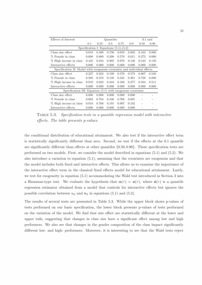
Table 5.3. Specification tests in a quantile regression model with interactive

effects. The table presents p-values.

the conditional distribution of educational attainment. We also test if the interactive effect term

is statistically significantly different than zero. Second, we test if the effects at the 0.1 quantile

are significantly different than effects at other quantiles 0.50, 0.90. These specification tests are

performed on two models. First, we consider the model described in equations (5.1) and (5.2). We

also introduce a variation to equation (5.1), assuming that the covariates are exogenous and that

the model includes both fixed and interactive effects. This allows us to examine the importance of

the interactive effect term in the classical fixed effects model for educational attainment. Lastly,

we test for exogeneity in equation (5.1) accommodating the Wald test introduced in Section 3 into

a Hausman-type test. We evaluate the hypothesis that α(τ) = a(τ), where a(τ) is a quantile

regression estimator obtained from a model that controls for interactive effects but ignores the

possible correlation between uit and vit in equations (5.1) and (5.2).

The results of several tests are presented in Table 5.3. While the upper block shows p-values of

tests performed on our basic specification, the lower block presents p-values of tests performed

on the variation of the model. We find that size effect are statistically different at the lower and

upper tails, suggesting that changes in class size have a significant effect among low and high

performers. We also see that changes in the gender composition of the class impact significantly

different low- and high- performers. Moreover, it is interesting to see that the Wald tests reject

24

the null hypothesis of no interactive effects in the model with fixed effects (p-values are 0.000). We

interpret this evidence as suggesting that the fixed effects specification is rejected in favor of the

interactive effects specification.

The lower block of Table 5.3 presents results for a series of Hausman-type exogeneity tests. It is

interesting to see that the tests reject the null hypothesis of exogeneity of class size in a model

conditional on interactive effects. In contrast, the tests suggest that class composition represented

by percentage of high-income students might be exogenous in our specification.

5.5. Improving Weak Students Performance

The previous analysis shows that for the poorly performing students, smaller classes appear to

be improving performance. In this section, we briefly investigate what is the class size reduction

needed to increase the achievement of these students at the bottom τL percentile in the conditional

distribution, to be at τ ′, with τ ′ > τL. In the case of two quantiles, the problem can be simply

formulated as minimizing y(τH)−y(τL) subject to y(τj) = q−c(τj)+αc(τj)dc, for τj = τL, τH. Thefunction q−c denotes the conditional quantile model corresponding to equation (5.1) that leaves out

the term αc(τj)dc. The variable dc is the number of students in class c and αc(τj) is the class-size

effect at the quantile τj. An additional constraint is that the total number of students S is split for

simplicity in two classes, c and c′. It is straightforward to show that the solution has the following

form:

d∗c =(q−c(τH)− q−c(τL)) + αc(τH)S

αc(τH) + αc(τL).

The implications of this expression are intuitive. Consider for simplicity the case of q−c(τH) =

q−c(τL). The solution d∗c suggests to have a class with few students if a reduction in the size of the

class does not significantly impact achievement at the highest quantile. If the effect of class size

does not change across the quantiles of educational attainment, the solution d∗c indicates to split

the students in classes of equal size.

Using Figure 5.2, we construct the percentage change in class size needed to increase the achieve-

ment of the weak-performing students at the bottom 10 percentile in the conditional distribution,

to be at τ = 0.11, 0.12, . . . , 0.5. For instance, the first point on the left represents the percentage

change in class size dc needed to increase the students’ score from the bottom 10 to the bottom

11 percentile of the conditional educational attainment distribution. We consider S = 268, which

is approximately twice the size of the average class in Table 5.1. We observe that most of the

point estimates are contained in the square in the left corner, suggesting that a small percentage

25

0.1 0.2 0.3 0.4 0.5

−0

.6−

0.4

−0

.20

.0

τ

pe

rce

nta

ge

ch

an

ge

cla

ss s

ize

Figure 5.2. Class size changes to prevent failure among the worst students.

reduction of about 10 percent can positively impact the worst students in class. We also observe

that the square in the top right corner of the plot is empty. This indicates that small reductions

in the size of the class cannot produce academic gains comparable to the median student. Notice

that making the weak performers comparable to the median performers does not seem to represent

a feasible policy, because the size of the class has to be reduced by 60 percent.

The estimation of effects at the lower tail of the conditional distribution provides a convenient tool

for the analysis of educational policies. Of course, one has to be cautious and interpret these results

within the context of conditional quantiles. The analysis of the effect of educational policies on

the unconditional attainment distribution is out of the scope of this paper and remains an open

question within the panel data quantile regression literature.

6. Conclusion

This paper proposes a quantile regression estimator for a model with interactive effects potentially

correlated with the independent variables and endogenous treatment effects. We provide conditions

26

under which the slope parameter estimator is consistent and asymptotically Gaussian. Monte Carlo

studies are carried out to investigate the finite sample performance of the proposed method in

comparison with other candidate methods. The evidence shows that the finite sample performance

of the proposed method is excellent under different Monte Carlo designs. We also apply the new

method to an investigation of the effect of class size on educational performance.

Several directions remain to be investigated. Inferential procedures could be implemented by ac-

commodating standard approaches, but they require a detailed investigation in the class of models

with interactive effects. Moreover, the presence of a large number of loadings and factors suggests an

attractive setting for regularization, which could represent an effective procedure to simultaneously

improve the performance of the method and do model selection.

Appendix A. Proofs

Proof of Proposition 1. (Consistency) Under the regularity conditions, identification and consis-

tency results immediately follows from the proof of Theorem 3 in Chernozhukov and Hansen (2006)

and Corollary 3.2.3 in van der Vaart and Wellner (1996). By proposition 2 in Chernozhukov and

Hansen (2008), we have that supα∈A ‖ϑ(α, τ) − ϑ(α, τ)‖ → 0 for ϑ = (β′, δ′,γ ′)′. This implies

that supα∈A ‖γ(α, τ) − γ(α, τ)‖ → 0, and that ‖α(τ) − α(τ)‖ → 0. Consider a small ball αn of

radius rn centered at α(τ). Then for any αn → α(τ), we have that β(αn, τ) → β(α(τ), τ) = β(τ),

δ(αn, τ) → δ(α(τ), τ) = δ(τ), and γ(αn, τ) → γ(α(τ), τ) = γ(τ) = 0. Hence ϑ(αn, τ) →ϑ(α(τ), τ) for any αn → α(τ).

(Asymptotic Normality) For any αn, we can write ρτ (yit−d′itα(τ)−x′

itβ(τ)−f ′t δ(τ)−w′

itγ(τ)) as

ρτ (yit− ξit(τ)−d′itδα/

√NT −x′

itδβ/√TN −f ′

tδλ/√NT −w′

itδγ/√NT ), where ξit(τ) = d′

itα(τ)+

x′itβ(τ) + f ′

tδ(τ) + w′itγ(τ), δα(αn, τ) =

√TN(α(αn, τ) − α(τ)), δβ(αn, τ) =

√TN(β(αn, τ) −

β(τ)), δλ(αn, τ) =√TN(δ(αn, τ)−δ(τ)), and δγ(αn, τ) =

√TN(γ(αn, τ)−0). Under assumption

4, the solution of (2.9) is equivalent to the solution of minimizing,

VTN (δ) =

T∑

t=1

N∑

i=1

ρτ

(

uit(τ)− d′it

δα√NT

− x′it

δβ√TN

− f ′t

δλ√TN

−w′it

δγ√NT

)

− ρτ (uit(τ))

where uit(τ) = yit − ξit(τ). Let,

(A.1) sup ||v(δα, δβ , δγ , δλ)− v(0,0,0,0) − E(v(δα, δβ , δγ , δλ)− v(0,0,0,0))|| = op(1)

27

where || · || denotes the standard Euclidean norm of a vector, ψτ (u) = τ − I(u < 0), and,

v(δα, δβ , δγ , δλ) =−1√TN

N∑

i=1

T∑

t=1

ftψτ

(

uit(τ)− d′it

δα√NT

− x′it

δβ√TN

− f ′t

δλ√TN

−w′it

δγ√NT

)

Taking expectation and expanding v under condition 6, we obtain

E(v(δα, δβ , δγ , δλ)− v(0,0,0,0)) =

= −E

(

1√TN

N∑

i=1

T∑

t=1

ftψτ

(

yit − d′it

δα√NT

− x′it

δβ√TN

− f ′t

δλ√TN

−w′it

δγ√NT

)

)

+1√TN

N∑

i=1

T∑

t=1

ftψτ (uit(τ))

)

= − 1√TN

N∑

i=1

T∑

t=1

ftgit(ξit(τ))

(

d′it

δα(τ)√NT

+ x′it

δβ√TN

+ f ′t

δλ√NT

+w′it

δγ√NT

)

+ o(1)

whereG(·) is the conditional distribution of y. Clearly, v(δα, δβ , δγ , δλ) → 0, and thus E(v(δα, δβ , δγ , δλ)−v(0,0,0,0)) = v(0,0,0,0). This last expression can be written as,

1√TN

N∑

i=1

T∑

t=1

ftgit(ξit(τ))

(

d′it

δα√NT

+ x′it

δβ√TN

+ f ′t

δλ√TN

+w′it

δγ√NT

)

=1√TN

N∑

i=1

T∑

t=1

ftψτ (uit(τ))

Letting f =∑N

i=1

∑Tt=1 git(ξit(τ))ftf

′t and solving for δλ, we have,

f ′t

δλ√TN

= f ′tf

−1

(

−N∑

i=1

T∑

t=1

ftgit(ξit(τ))(

d′it

δα√NT

+ x′it

δβ√TN

+w′it

δγ√NT

)

+

N∑

i=1

T∑

t=1

ftψτ (uit(τ))

)

+Rit√TN

= −dt(τ)′ δα√TN

− xt(τ)′ δβ√TN

− wt(τ)′ δγ√TN

+ f−1N∑

i=1

T∑

t=1

ftψτ (uit(τ)) +Rit√NT

where for instance dt(τ) = f ′tf

−1∑N

i=1

∑Tt=1 git(ξit(τ))ftdit, and Rit is the remainder term. Sub-

stituting the λ’s we denote,

v(δα, δβ , δγ) =−1√NT

N∑

i=1

T∑

t=1

hitψτ

(

uit(τ)− d′it

δα√NT

− x′it

δβ√TN

− f ′t

δλ√NT

−w′it

δγ√NT

)

where hit = (x′it,w

′it)

′. By uniformity,

(A.2) sup ||v(δα, δβ , δγ)− v(0,0,0) − E(v(δα, δβ , δγ)− v(0,0,0))|| = op(1)

28

Expanding as above we obtain

E(v(δα, δβ , δγ)− v(0,0,0)) =

= − 1√TN

T∑

t=1

N∑

i=1

hitgit(ξit(τ))

(

d′it

δα√NT

+ x′it

δβ√TN

+w′it

δγ√NT

−dt(τ)′ δα(τ)√TN

− xt(τ)′ δβ√TN

− wt(τ)′ δγ√TN

+ f−1N∑

i=1

T∑

t=1

ftψτ (uit(τ)) +Rit√NT

)

Notice that v(δα, δβ , δγ) → 0, and thus E(v(δα, δβ , δγ) − v(0,0,0)) = v(0,0,0). Letting δϑ =

(δ′β , δ′γ)

′, we write the last expression as,

1√TN

T∑

t=1

N∑

i=1

hitgit

(

(d′it − d′

t(τ))δα(τ)√NT

+ (h′it − h′

t(τ))δϑ(τ)√TN

+ f−1N∑

i=1

T∑

t=1

ftψτ (uit(τ)))

=

1√TN

T∑

t=1

N∑

i=1

hitψτ (uit(τ))−Rit√NT

Alternatively, using more convenient notation, we write the last expression as, Jαδα + Jϑδϑ =

Jψ −R, where Jα = limN,T→∞ H ′M ′FΦMFD, Jϑ = limN,T→∞ H ′M ′

FΦMFH , and Jψ is a mean

zero random variable with covariance τ(1− τ)H ′M ′FMF H. The remainder term R is op(1) under

the regularity conditions. Letting [J ′β, J

′γ ]

′ be a conformable partition of J−1ϑ as in Galvao (2009)

and Chernozhukov and Hansen (2006), then, δγ = J ′γ(Jψ − Jαδα), and δβ = J ′

β(Jψ − Jαδα).

LettingH = J ′γAJγ as in Chernozhukov and Hansen (2006), we have that δα = (J ′

αHJα)−1J ′

αHJψ .

Replacing it in the previous expression,

δγ = J ′γ(Jψ − Jαδα) = J ′

γ(I − Jα(J′αHJα)

−1(J ′αH))Jψ = J ′

γ(I −L)Jψ = J ′γMJψ

where L = Jα[J′αHJα]

−1J ′αH andM = I−L. Due to invertibility of JαJγ , δγ = 0×Op(1)+op(1).

Similarly, substituting back δα, we obtain that δβ = J ′β(I − L)Jψ. By the regularity conditions,

we have that,

δ =

(

δα(αn, τ)

δβ(αn, τ)

)

=

( √TN(α(αn, τ)−α(τ))√TN(β(αn, τ)− β(τ))

)

N(

0,J ′SJ)

.

29

References

Abrevaya, J., and C. Dahl (2008): “The Effects of Smoking and Prenatal Care on Birth Outcomes: Evi-

dence from Quantile Regression Estimation on Panel Data,” Journal of Business and Economics Statistics,

26(4), 379–397.

Ando, T., and R. S. Tsay (2010): “Quantile Regression Models with Factor-Augmented Predictors and

Information Criterion,” Econometrics Journal, forthcoming.

Angrist, J., and V. Lavy (1999): “Using Maimonides’ Rule to Estimate The Effects of Class Size on

Scholastic Achievement,” Quarterly Journal of Economics, 114, 533–575.

Bai, J. (2009): “Panel Data Models with Interactive Fixed Effects,” Econometrica, 77(4), 1229–1279.

Baltagi, B. (2005): Econometric Analysis of Panel Data. Wiley, New York, 3nd edn.

Bandiera, O., V. Larcinese, and I. Rasul (2010): “Heterogeneous Class Size Effects: New Evidence

from a Panel of University Students,” forthcoming, Economic Journal.

Canay, I. (2010): “A Note on Quantile Regression for Panel Data Models,” mimeo, Northwestern University.

Chernozhukov, V., I. Fernandez-Val, and W. Newey (2009): “Quantile and Average Effects in

Nonseparable Panel Models,,” cemmap Working Papers, CWP29/09.

Chernozhukov, V., and C. Hansen (2005): “An IVModel of Quantile Treatment Effects,” Econometrica,

73(1), 245–262.

(2006): “Instrumental quantile regression inference for structural and treatment effect models,”

Journal of Econometrics, 132(2), 491–525.

(2008): “Instrumental variable quantile regression: A robust inference approach,” Journal of Econo-

metrics, 142(1), 379–398.

Coleman, J. (1966): “Equality of Educational Opportunity,” Report for US Department of Health, Edu-

cation, and Welfare, Office of Education, Washington D.C.

De Giorgi, G., M. Pellizzari, and W. Woolston (2009): “Class-size and Class Heterogeneity,” mimeo,

Stanford University.

DiNardo, J., and D. S. Lee (2010): “Program Evaluation and Research Designs,” NBER WP 16016.

Doksum, K. (1974): “Empirical Probability Plots and Statistical Inference for Nonlinear Models in the

Two-Sample Case,” Annals of Statistics, 2, 267–277.

Galvao, A. (2009): “Quantile Regression for Dynamic Panel Data with Fixed Effects,” mimeo, University

of Illinois at Urbana-Champaign.

Graham, B. S., J. Hahn, and J. L. Powell (2009): “The Incidental Parameter Problem in a Non-

differentiable Panel Data Model,” Economics Letters, 105, 181–182.

Hanushek, E. A., J. F. Kain, J. M. Markman, and S. G. Rivkin (2003): “Does Peer Ability Affect

Student Achievement?,” Journal of Applied Econometrics, 18, 527–544.

Harding, M., and C. Lamarche (2009): “A Quantile Regression Approach for Estimating Panel Data

Models Using Instrumental Variables,” Economics Letters, 104, 133–135.

Hausman, J. A. (1978): “Specification Tests in Econometrics,” Econometrica, 46(6), 1251–1271.

Heckman, J. J., and E. Vytlacil (2001): “Policy-Relevant Treatment Effects,” American Economic

Review, 91(2), 107–111.

30

Hoxby, C. (2000): “The Effects of Class Size on Student Achievement: New Evidence from Population

Variation,” Quarterly Journal of Economics, 115, 1239–1285.

Hsiao, C. (2003): Analysis of Panel Data. Cambridge University Press, New York, 2nd edn.

Kato, K., and A. F. Galvao (2010): “Smoothed Quantile Regression for Panel Data,” mimeo, Hiroshima

University.

Koenker, R. (2004): “Quantile Regression for Longitudinal Data,” Journal of Multivariate Analysis, 91,

74–89.

(2005): Quantile Regression. Cambridge University Press.

(2010): “Quantreg,” R package version 4.48, www.r-project.org.

Koenker, R., and G. Bassett (1982): “Tests of Linear Hypothesis and ℓ1 Estimation,” Econometrica,

50, 1577–1584.

Koenker, R., and S. Portnoy (1987): “L-estimation for Linear Models,” Journal of the American

Statistical Association, 82, 851–857.

Koenker, R., and Z. Xiao (2002): “Inference on the Quantile Regression Process,” Econometrica, 70,

1583–1612.

Krueger, A. B. (1999): “Experimental Estimates of Education Production Functions,” Quarterly Journal

of Economics, 114, 497–532.

Lamarche, C. (2010): “Robust Penalized Quantile Regression Estimation for Panel Data,” Journal of

Econometrics, 157, 396–408.

Lehmann, E. (1974): Nonparametrics: Statistical Methods Based on Ranks. Holden-Day Inc.

Levin, J. (2001): “For Whom the Reductions Count: A Quantile Regression Analysis of Class Size and

Peer Effects on Scholastic Achievement,” Empirical Economics, 26, 221–246.

Ma, L., and R. Koenker (2006): “Quantile Regression Methods for Recursive Structural Equation Mod-

els,” Journal of Econometrics, 134, 471–506.

Newey, W. K. (1991): “Uniform Convergence in Probability and Stochastic Equicontinuity,” Econometrica,

59, 1161–1167.

Pesaran, M. H. (2006): “Estimation and Inference in Large Heterogeneous Panels with a Multifactor Error

Structure,” Econometrica, 74(4), 967–1012.

Ponomareva, M. (2010): “Quantile Regression for Panel Data Models with Fixed Effects and Small T:

Identification and Estimation,” mimeo, University of Western Ontario.

Powell, D. (2009): “Unconditional Quantile Regression for Panel Data with Exogenous or Endogenous

Regressors,” Rand Working Paper WR-710.

Rosen, A. (2009): “Set Identification via Quantile Restrictions in Short Panels,” CEMMAP, WP 26/09.

Ruppert, D., and R. Carroll (1980): “Trimmed Least Squares Estimation in the Linear Model,” Journal

of the American Statistical Association, 75, 828–838.

van der Vaart, A. W., and J. A. Wellner (1996): Weak Convergence and Empirical Processes.

Springer, New York.

Wei, Y., and X. He (2006): “Conditional Growth Charts,” Annals of Statistics, 34(5), 2069–2097.