CARMA Memorandum Series #63

CARMA Summer School 2014

Melvyn Wright, Marc Pound, Dick Plambeck, John Carpenter,Doug Friedel, Nikolaus Volgenau, Patrick Kelly, Lauranne Lanz,Lauren McKeown, Jay Franck, Erin Cox, Maryam Tabeshian,

Andrew Nadolski, Dana Anderson, Scott Barenfeld, DevinCrichton, Ko-Yun Huang, Jonathan Florez, Amy Steele, NedMolter, Joey Rodriguez, Bandon Decker, Shravan Avadhuta

October 10, 2014

ABSTRACT

The 8th CARMA Summer School was held at the observatory at Cedar Flat 2014on Aug 3-Aug 9, 2014 with 18 students from Berkeley, Caltech, Illinois, Maryland,Johns Hopkins, Vanderbilt, Fisk, Wesleyan, Trinity College Dublin, Missouri, Cal State,Macalaster, Western Ontario, and Case Western Reserve. A new wrinkle this year isthat youtube channel of the lectures was set up for three international students who wereunable to attend. The channel was quite successful until Google shut it down, claimingviolation of community guidelines. Poor weather hampered observations during the firstcouple days, but there was still enough good weather during the rest of the week forstudents to get plenty of data.

During the school, students formed small teams and designed and obtained their ownobservations, in consultation with the instructors. Using both science subarrays studentsobserved star-forming regions, YSOs and outflows, Saturn, stellar atmospheres, nearbygalaxies, a high-z galaxy, and galaxy clusters. At the end of the week, the studentsgave short presentations on their results. In this memo we collect together some of theresults from the student projects.

– 2 –

1. Introduction

The 8th CARMA Summer School was held at the observatory at Cedar Flat on Aug 3-Aug 9, 2014with 18 students and 6 instructors. As in previous years, the school had the use of the telescope forthe week. The array was in the most compact E-configuration. During the school the students hadtheir own observing projects which they worked on during the week as well as attending lecturesand demonstations. Each of the student projects had 5-6 hours of telescope time and the studentscontrolled the telescope for their own projects. The students took the observations, reduced andanalyzed the data, and presented the results.

On the first day the students learned how to select suitable observing projects for the CARMAtelescope. The introductory lectures covered the characteristics of the telescope, instrumentation,and observing techniques which taught the students to:

select suitable astronomical sources for observing.

select the observing frequency, spectral lines to be observed.

evaluate angular resolution, velocity resolution and sensitivity needed.

select the correlator setup and calibrations needed.

prepare an observing script to define the observing procedure at the telescope.

make the observations

During the rest of the week, the lectures and demonstrations covered the theory and techniquesused for millimeter wavelength aperture synthesis and for the CARMA array, and more detailedlectures on the hardware and software, and reducing and analyzing data. As they worked on theirprojects the students learned how to:

schedule the telescope effectively.

calibrate the data.

make images.

identify and fix problems that set off the alarm.

analyze and present the results.

On Friday the students made 10-15 minute presentations and we discussed the results. In all, avery satisfying week seeing all the enthusiasm and so many exciting projects from initial planningand observations, to analysis and results.

– 3 –

2. The CARMA Telescope

The CARMA telescope is an aperture synthesis array, typically operating as two independentsubarrays of 15 and 8 antennas, respectively. In the CARMA-15 subarray, there are two receiverbands, 3 mm and 1 mm, and the spectral line correlator. A basic aperture synthesis observationmakes an image the size of the the primary beam (λ/D ∼1′ at 100 GHz; 0.5′ at 230 GHz) with aresolution corresponding to the maximum separations of the antennas. During the Summer School,CARMA-15 was in the E configuration, with an angular resolution ∼ 10′′ at 100 GHz, and ∼ 5′′

at 230 GHz. The CARMA-8 subarray of eight 3.5m antennas was in the SL configuration forcontinuum-only projects at 30 GHz (primary beam ∼ 11′; resolution ∼ 2′) and 90 GHz (primarybeam ∼ 3.6′; resolution ∼ 40′′). The CARMA-8 correlator produces 7 GHz of continuum data. Allantennas can be combined into a single 23-element array, CARMA-23, with 4 GHz of correlatorbandwidth.

It’s best to observe a strong enough source that one can make an image during the school, ratherthan a detection project, then the effects of different imaging techniques can be explored. Themost convenient source size is one which is smaller than the size of the primary beam when onlyone pointing is needed. Larger sources can be imaged by time-sharing the pointing of the antennas(mosaicing), at the cost of lowered sensitivity.

The sensitivity is determined by the system noise (receivers plus atmosphere), the bandwidth (orvelocity resolution), and the observing time. The atmosphere is usually not so good for 1 mmobservations in the summer (although a couple 1 mm projects were run this year), for sourceswhich are at low declinations that must be observed through more of the atmosphere, so select abright source which is high in the sky and can be observed at 3 mm or 1 cm is preferred. Not all theprojects that the students wanted to do satisfied these these conditions, so a final list of projectsfrom those proposed was selected on the first day of the school. Students grouped themselves intosmall teams to work on the selected projects.

2.1. Logistics

Because this is a hands-on school, all lectures and demonstrations were held in the control buildingand at the telescopes at Cedar Flat. Mel, Marc, Dick, Doug, and 16 of the students stayed in the“Noren” group campground, about 1.5 miles from the control room, and near the antenna pads forthe A-configuration. Those who camped avoided the hassle of driving up and down the mountaineach day and had a wonderful opportunity to fall asleep under a star-filled and moonless sky eachnight. The other students stayed in the dorm and cottage at OVRO. Delicious breakfasts, lunches,and dinners were provided at the observatory, prepared by Sarah Landry and Barbara Marzano.Mary Daniel adroitly handled all the accomodations, making sure every one had a place to resttheir weary heads at the end of the long days. We organized a hike to Second Lake on Saturday.

– 4 –

3. Mapping the Structure of the L1157-mm Stellar OutflowShravan Avadhuta (CSU-LA) & Scott Barenfeld (Caltech)

3.1. Introduction

Protostars are surrounded by an envelope of gas and dust accreting onto the still-forming star. Notall of this material makes it onto the star, however. A significant fraction is expelled from the polesof the star, forming a large, bipolar outflow. A classic example of such a system is the well-studiedL1157-mm (e.g. Stephens et al. (2013)). Millimeter wavelength observations are sensitive to thethermal emission of the dust in these systems, as well as the CO rotational transitions. As such,we use the CARMA interferometer to study the structure of L1157-mm at a wavelength of 3 mm.

3.2. Observations and Data Reduction

Observations of L1157-mm were carried out using the 15 10.4 m and 6.1 m antennas of the CARMAarray in E configuration. The correlator was divided into three 31 MHz windows, centered on the12CO, 13CO, and C18O (1-0) transitions, and five 500 MHz continuum windows. Observationsstarted on August 11th 2014 at 11:30 pm and continued until August 12th 3:30 am, PST. Theweather during the observation was not very favorable with average τ of 1.573 and Phase RMS of327 µm. 3C84 was used as a bandpass calibrator, Uranus as a flux calibrator, and 1927+739 as again calibrator. Despite the weather conditions, the track proceeded without any alarms. The datarequired very little flagging except for a few outlying amplitudes for our calibrators. The data werecalibrated and maps were generated using the automated scripts provided by John Carpenter.

3.3. Results and Discussion

3.3.1. Dust Continuum

The integrated map generated from our continuum windows is shown in Figure 1. This continuumemission traces the location of dust within the system, which appears to be centrally located withinthe central 10” of the young star. Fitting an elliptical Gaussian to the emission in this region, wefind an integrated flux density of 81.6 mJy.

3.3.2. 12CO

Our 31 MHz spectral window centered on 115.271 GHz is sensitive to the 12CO (1-0) transition. Ourmap of this window shows the bipolar outflow structure of L1157-mm (Figure 2). To investigate thestructure of this outflow in velocity space, we integrated 1.25 km/s sections of the 12CO window for

– 5 –

all channels showing 12CO emission upon visual inspection. We see emission for velocities between13.8 km/s below and 6.6 km/s above 115.271 GHz. Note that L1157-mm is moving away from theSun with a velocity of several km/s, so it is not unexpected that the above velocity range is notsymmetric about 115.271 GHz. Stepping through velocity space, Figure 3 shows that the upperlobe in the outflow is moving with positive velocity (redshifted) with respect to the the centralprotostar, while the lower lobe is moving with negative velocity (blueshifted). Figure 4 shows theintegrated fluxes of all channels showing the upper lobe and all channels showing the lower lobe,respectivley. The velocity structure of the outflux indicates it is inclined relative to the line of sight,with the upper lobe tilted away from Earth and the lower lobe towards Earth.

3.3.3. 13CO and C18O

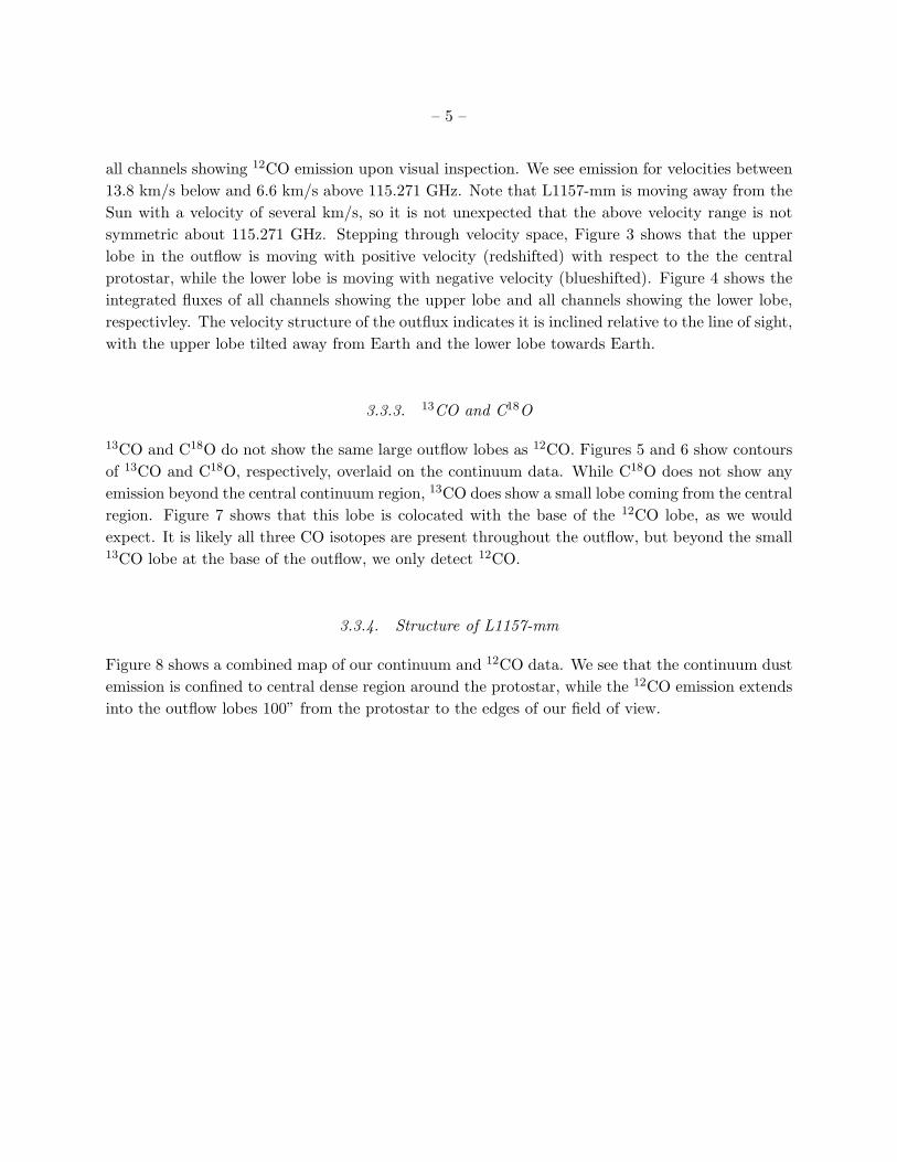
13CO and C18O do not show the same large outflow lobes as 12CO. Figures 5 and 6 show contoursof 13CO and C18O, respectively, overlaid on the continuum data. While C18O does not show anyemission beyond the central continuum region, 13CO does show a small lobe coming from the centralregion. Figure 7 shows that this lobe is colocated with the base of the 12CO lobe, as we wouldexpect. It is likely all three CO isotopes are present throughout the outflow, but beyond the small13CO lobe at the base of the outflow, we only detect 12CO.

3.3.4. Structure of L1157-mm

Figure 8 shows a combined map of our continuum and 12CO data. We see that the continuum dustemission is confined to central dense region around the protostar, while the 12CO emission extendsinto the outflow lobes 100” from the protostar to the edges of our field of view.

– 6 –

Fig. 1.— Continuum emission at 3mm of L1157-mm, corresponding to dust. The dust is concen-trated in the central region around the protostar, and does not appear in the outflow.

– 7 –

Fig. 2.— 12CO (1-0) emission. The CO traces the outflow from the protostar.

– 8 –

Fig. 3.— 12CO (1-0) emission maps integrated over every 1.25 km/s. The positive (redshifted)velocites show emission in the upper lobe, while the negative (blueshifted) velocities show emissionin the lower lobe. This indicates the outflow is inclined with respect to Earth, with the upper lobetilted away.

– 9 –

Fig. 4.— 12CO (1-0) contours for the integrated positive velocities (red) and negative velocities(blue). Dust continuum emission is shown in green.

– 10 –

Fig. 5.— 13CO (1-0) contours (red) overlaid on the continuum emission (green). 13CO is visible inthe central envelope, as well as in the base of the lower part of the outflow.

– 11 –

Fig. 6.— C18O (1-0) contours (red) overlaid on the continuum emission (green). No C18O is visibileoutside of the central envelope.

– 12 –

Fig. 7.— 13CO (1-0) contours (green) overlaid on the 12CO (1-0). The outflow structure of 13COtraces the lower 12CO outflow.

– 13 –

Fig. 8.— 12CO (1-0) contours (red) overlaid on the continuum (green). This shows the combinedenvelope and outflow structure of L1157-mm.

– 14 –

4. Looking for Molecular Gas in NGC 1052Lauranne Lanz (Caltech)

4.1. Introduction

4.1.1. Molecular Gas in Elliptical Galaxies

An important difference between spiral and elliptical galaxies is their molecular gas content. Thecanonical view of galaxy evolution broadly requires that gas-rich spirals eventually become, throughsecular or merger processes, gas-poor ellipticals. We therefore expect that there should exist tran-sitional objects, such as ellipticals with significant molecular content. Such galaxies provide animportant insight into a crucial period in galaxy evolution. The ATLAS3D (Cappellari et al. 2011)sample of early-type galaxies was observed with CARMA (Alatalo et al. 2013), which showed avariety of CO morphology, including disks, spiral arms, and disturbed morphologies.

4.1.2. NGC 1052

NGC 1052 is a nearby (z=0.0050, 22 Mpc) early type galaxy with a compact, flat-spectrum radiocore and a two-sided radio jet contained within the host galaxy. It belongs to a class of galaxiesknown as Molecular Hydrogen Emission Galaxies (MOHEGs; e.g., Ogle et al. 2010), whose mid-IR spectrum show strong H2 emission relative to their polycyclic aromatic hydrocarbon (PAH)emission. Both PAH and H2 emission may be excited by UV photons from young stars. However,the large ratio of H2/PAH emission in these galaxies indicate that the energetic source of the H2

emission cannot be star formation. Analysis of MOHEGs that are also radio galaxies (e.g., Guillardet al. 2012; Ogle et al. 2010) suggests that the most likely excitation mechanism of the moleculargas to the observed 100-1000 K temperatures are shocks driven into the interstellar medium (ISM)by the radio jets. Mapping the molecular gas using CARMA provides insights into the coldermolecular gas and whether it also shows indications of interactions with the radio jet. Further, themass and extent of the molecular gas are necessary to determine whether the radio jet has quenchedstar formation in this galaxy by accurately determining where on the Kennicutt-Schmidt diagramthis galaxy falls.

4.2. Observations and Data Reduction

NGC 1052 was observed using the CARMA-15 subarray in the compact (E) configuration on 5August 2014. While the optical diameter of the galaxy (69′′; Wang et al. 1992) is similar in extentto the size of the 10 m primary beam, we did not expect to detect emission on the outskirts ofthe galaxy. Therefore, we chose to concentrate our observing time in a single pointing centeredon the VLBA position of α = 02:41:04.80 and δ = −08:15:20.75 (Beasley et al. 2002). From a

– 15 –

single-dish observation (Nobeyama 45 m; Wang et al. 1992), we expected the 12CO to be about∼ 100 km s−1 wide. Since we wanted to detect the structure of the line, we chose our correlatorsettings to balance velocity coverage and sufficient velocity resolution to detect line structure. Wetherefore placed a 125 MHz spectral window centered to have the 12CO line in the upper side bandat 115.27 GHz. Additionally, we placed three other 125 MHz spectral windows centered on the13CO line at 110.20 GHz, the CN line at 113.49 GHz, and the CS line at 97.98 GHz. We placed250 MHz windows on the 18CO line at 109.78 GHz and the CN line at 113.19 GHz. The remainingtwo windows were kept as 500 MHz continuum windows. The local oscillator frequency was set at109.235 GHz.

The observation track ran for 4.8 hours. NGC 1052 was observed for hours, with the remaining timespent on calibration objects and pointing targets. Our calibration objects were: Uranus for flux, thequasar 0224+069 for gain, and 3C84 for passband. The sky was clear during the observation, but theatmosphere showed some turbulence with a typical RMS of 500µm and τ230GHz =0.95. The bulkof the data reduction was done using John Carpenter’s MIRIAD script. Very little flagging provednecessary. Due to the brightness of the continuum of NGC 1052, we elected to self-calibrate thepassbands rather than using 3C84, which also showed greater amplitude variations. Additionally,we chose to use natural weighting since the source did not appear particularly extended.

4.2.1. Ancillary Data

We wanted to determine where the sub-millimeter emission fell relative to the stellar, dust, hotgas, and radio jet emission of NGC 1052. For the stellar emission comparison, we obtained a g-band image from the SDSS DR10 archive. We were in possession of a 70µm image taken withthe PACS instrument on the Herschel Space Observatory. This mosaic was created using thesoftware Scanamorphos (Roussel 2013) from data in the Herschel Science Archive. For the hot gascomparison, we reprocessed the Chandra X-ray Observatory observation taken from the ChandraArchive using the CIAO software (v. 4.5; Fruscione et al. 2006). A Very Large Array image takenas part of the FIRST survey was also acquired (D. Crichton, priv. comm.).

4.3. Results and Discussion

4.3.1. 3mm Continuum

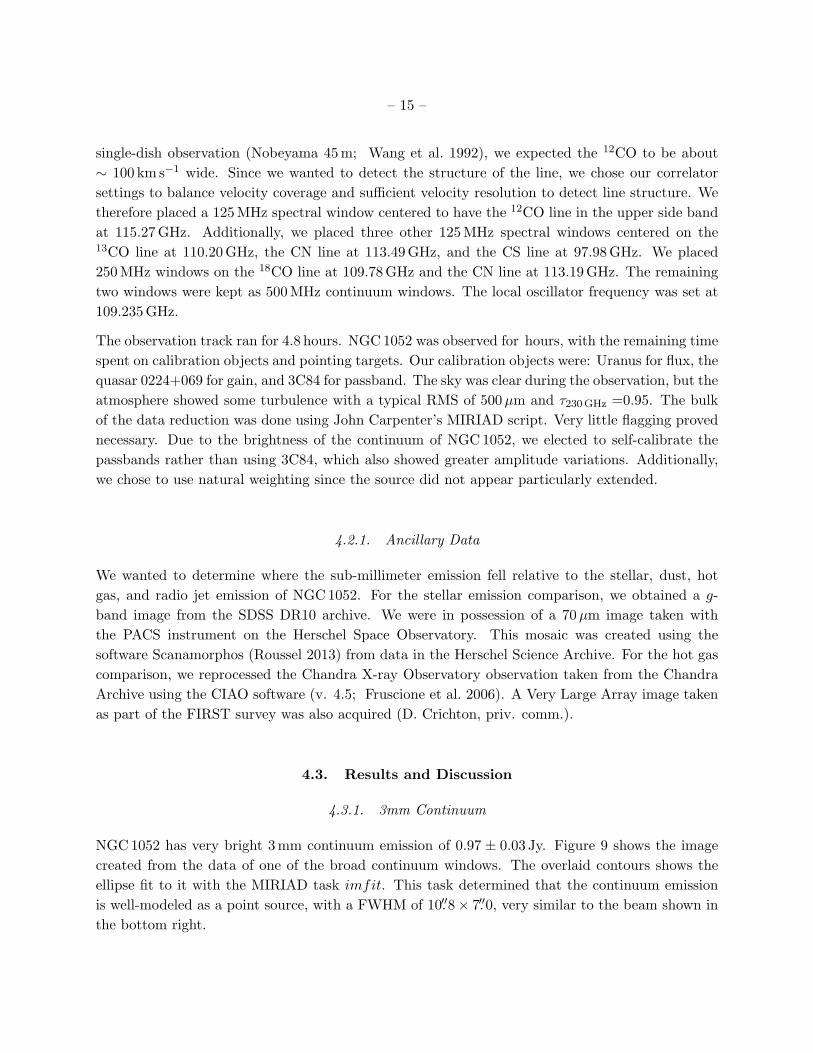
NGC 1052 has very bright 3 mm continuum emission of 0.97 ± 0.03 Jy. Figure 9 shows the imagecreated from the data of one of the broad continuum windows. The overlaid contours shows theellipse fit to it with the MIRIAD task imfit. This task determined that the continuum emissionis well-modeled as a point source, with a FWHM of 10.′′8× 7.′′0, very similar to the beam shown inthe bottom right.

– 16 –

Fig. 9.— Continuum map of NGC 1052 overlaid with contours derived by imfit, showing theemission to be point-like.

– 17 –

In extragalactic observations, 10′′ can extend across much of a distant galaxy or describe the verycenter of a galaxy. As such, we want to establish whether a submillimeter source unresolved withthis configuration of CARMA is confined to the nuclear region or could extend over a significantfraction of the galaxy. Figure 10 overlays the contours of SDSS g-band emission showing the stellarextent (Fig. 10a), the PACS 70µm emission showing the dust (Fig. 10b), the broadband (0.5-8 keV) Chandra emission showing the AGN and hot gas emission (Fig. 10c), and the VLA emissionshowing the radio jets (Fig. 10d). These images demonstrate that the submillimeter emission isconfined to the central region of the galaxy and, may well be associated with the AGN. Fig. 10cin particular shows that the submillimeter and central X-ray point source are spatially coincident.Similarly, the positions of the radio core and continuum point source agree.

(a)

30"

(c) (d)

15"

(b)

Fig. 10.— Continuum map of NGC 1052 overlaid with contours from (a) SDSS g, (b) PACS 70µm,(c) Chandra 0.5-8 keV, and (d) VLA 1.4 GHz. The latter three are on a smaller scale within theyellow box shown in (a). The mix of black and white contours is purely to improve visibility.

– 18 –

4.3.2. 12CO(1-0) Emission

We tried two methods for detecting the 12CO(1-0) line. First, we extracted the spectrum in theclean map of the spectral window containing the 12CO(1-0) line using imspec and subtracted thecontinuum determined from the average of the channels on both sides of the expected position ofthe lines. The result is shown in Figure 11. While there exists a spectral feature at the velocityexpected from the Nobeyama observation (Wang et al. 1992), the fact that it is only the width ofone 8 km s−1 channel is concerning. Therefore, we tried a second extraction method, wherein wesubtract the average of the dirty maps in the wide continuum windows from the dirty map of the12CO(1-0) window. This subtraction must be done with the dirty maps rather than the cleanedmaps, because the deconvolution process used in cleaning is non-linear. Since the two sets of dirtymaps should have similar side lobe features, the subtraction will also do a simple cleaning on thespectral map. Indeed, we find that the maps of the continuum windows are have very little inthe way of residuals once their average is subtracted from them. We extracted the spectrum inthe subtracted map and find a spectrum very similar to that shown in Figure 11. At this time,whether emission in the 12CO(1-0) line has been significantly detected remains unclear. However,if the spectral feature seen in Figure 11 does accurately reflect that emission, then it has a similarspatial morphology to the continuum, albeit a much weaker detection.

4.3.3. Future Work

An important lesson learned from this project is that, for extragalactic observations, the correlatorspectral windows are best kept at 500 MHz. We obtained a second observation of NGC 1052 justafter the end of the CARMA school on 9 August 2014, with better correlator settings, with whichwe hope to significantly detect the 12CO line.

– 19 –

Fig. 11.— Continuum-subtracted spectrum in the 12CO(1-0) window.

– 20 –

5. Millimeter Observations of RW Aurigae: Searching for Disrupted CircumstellarMaterial

Joseph E. Rodriguez Jr. (Vanderbilt University)

5.1. Introduction

The circumstellar environment of young stellar objects (YSOs) involves dynamical interactions be-tween gas and dust. The gas and dust typically orbit in a circumstellar disk, and can be inferredby an excess of infrared radiation. Observing the environment of YSOs and how the gas and dustinteract, can provide us with crucial information to better understand the processes of planetaryformation. An extreme example of a YSO environment is the classical T-Tauri star, RW Aurigae.Cabrit et al. (2006) performed millimeter observations of the RW Aurigae system, providing evi-dence that the system had undergone a reconfiguration of its circumstellar environment. As RWAur B orbited close to the primary component, RW Aur A, it disrupted the surrounding circum-stellar material of RW Aur A. This material has now co-allesed into a large tidal arm, wrappedaround RW Aur A (Figure 12). In 2010, the system dimmed by ∼2 magnitudes (in the V -band)for a duration of 180 days (Figure 13). It is believed that this dimming was caused by a portionof disrupted material, from the system’s violent history, occulting the RW Aur A (Rodriguez et al.2013).

The Rayleigh-Jeans approximation, Fν ∼ ν2+β, allows us to combine the measured total flux inmillimeter observations to infer properties of the circumstellar environment of RW Aurigae. If β ismeasured to be around 2, this is indicative of an optically thin disk and likely no grain growth. Ifβ is less than 1, this suggests the circumstellar material is optically thick and possibly undergoinggrain growth through collisions.

5.2. Observations and Data Reduction

We observed the RW Aurigae system using the Combined Array for Research in Millimeter Astron-omy (CARMA) for ∼3.2 hours. Specifically, we used the CARMA 15 E configuration consistingof nine 6.1m and six 10.4m antennas. All observations were taken on August 7th, 2014 betweenLocal Sidereal Time 0h and 5h. Along with observing RW Aurigae, we observed Uranus, 3C84 and0510+180 as the flux, passband and gain calibrator, respectively. Due to inadequate weather for1mm observing, we observed in the 3mm continuum. The observations and maps presented herewere reduced using the MIRIAD software program, described in detail by Sault et al. (1995).

5.3. Results and conclusion

Using the CARMA 15 E array, we hoped to accomplish a few goals along with the learning expe-rience that the CARMA summer school provided. First, we would like to expand on the IRAM

– 21 –

1.3mm map that Cabrit et al. (2006) presented, looking for previously undetected material. Second,combining our observations with previous mm observations, we are able to tentatively interpret thepresence of grain growth.

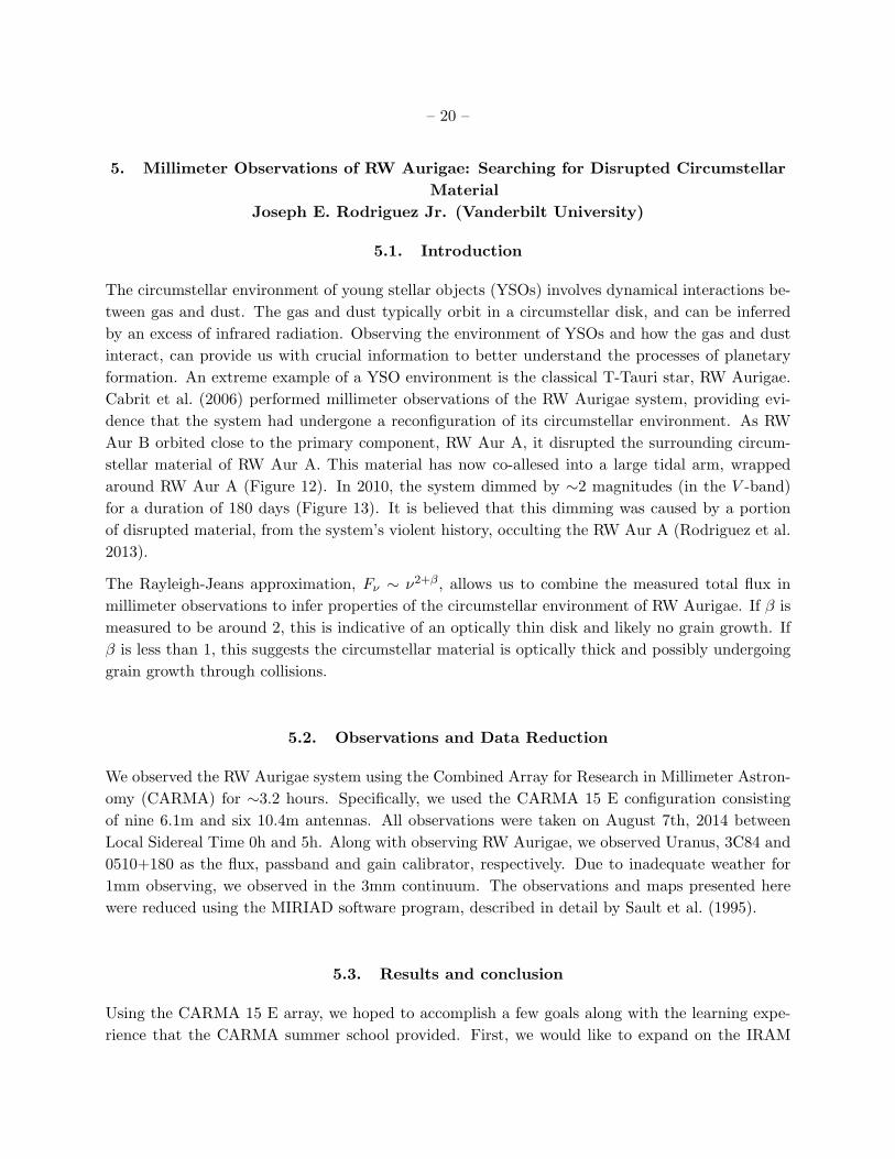
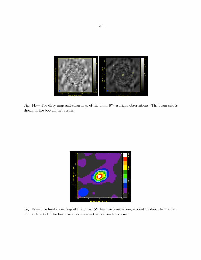
In Figure 14, both the dirty and clean 3mm maps are presented. By “Dirty Map”, we are referringto the uncalibrated, unprocessed, raw data that is outputting but the array. The “Clean Map” hasbeen fully calibrated and poor data has been flagged and removed from the reduction. The cleanmap shows a clear detection of the RW Aur system. Figure 15 presents the final cleaned map,using a color scaling to show the true contours of the detection. This plot is also zoomed in to showthe nearby area surrounding the RW Aur system. In our final map, we clearly detect RW Aur butonly as a point source. There appears to be some elongation but this is not statistically significantwhen compared to the beam size.

We are able to calculate the total flux of RW Aur in the 3mm continuum to be 6.24 ± 0.2 mJy.Previous results by Cabrit et al. (2006) measured a total flux in the 1.3mm band to be 32.8 ± 0.7mJy with 0.89′′ resolution. Osterloh & Beckwith (1995) found the 1.3mm flux to be 42.5 ± 5 mJywith a 12′′ beam. Keeping the beam sizes consistent, we combine our measurements here with theOsterloh & Beckwith (1995) measured flux to estimate the value of β in the equation presentedabove. We calculate that β ∼ 0.25±0.2. Even though the error on our observations is quite high,our value of β is consistent with an optically thick disk and may indicate the presence of graingrowth. If the proposed violent history of the RW Aur system is correct, that RW Aur B is on aneccentric orbit and during the last fly-by it significantly disrupted the circumstellar material aroundRW Aur A, it would likely increase the amount of grain collisions. Therefore, it is possible that theinteraction increased grain growth and our calculated value of β is indicative of that. However, wecan not claim the presence of grain growth without more definitive results.

– 22 –

Fig. 12.— Figure 1 from Cabrit et al. (2006) showing the a) 12CO(2-1) emission, b) 12CO(2-1)centriod, c) 1.3mm continuum and d) 12CO(2-1) width maps of the RW Aurigae system fromIRAM.

Fig. 13.— Figure 1b from Rodriguez et al. (2013) showing a large dimming event from 2010 to2011. Plotted are the KELT-North, SuperWASP and AAVSO light curves from the KELT-Northobserving seasons.

– 23 –

Fig. 14.— The dirty map and clean map of the 3mm RW Aurigae observations. The beam size isshown in the bottom left corner.

Fig. 15.— The final clean map of the 3mm RW Aurigae observation, colored to show the gradientof flux detected. The beam size is shown in the bottom left corner.

– 24 –

6. CO emission in the famous dwarf irregular galaxy IC 2574Ned Molter (Macalester College) and Amy Steele (University of Maryland)

6.1. Introduction

The low mass and metallicity of dwarf galaxies make them local analogs to galaxies at high redshift,meaning that studying the local dwarf galaxy population is essential to understanding galaxyformation and evolution in the early Universe. In particular, star-forming dwarf irregular galaxiesaid our understanding of the way star formation proceeds in the low metallicity regime, where gasclouds are less abundant in heavy molecules like CO. The tight relationship between moleculargas and star formation (Bigiel et al. 2008) suggests that such molecules play an essential role inradiating energy out of a molecular gas cloud, cooling it and allowing it to collapse. However,gas cloud collapse and star formation must also have occurred in Population III stars with zerometallicity, and the details of this process are constrained only theoretically—no empirical evidenceexists. Metal-deficient dwarf galaxies are therefore a crucial test bed for star formation processesat low metallicities.

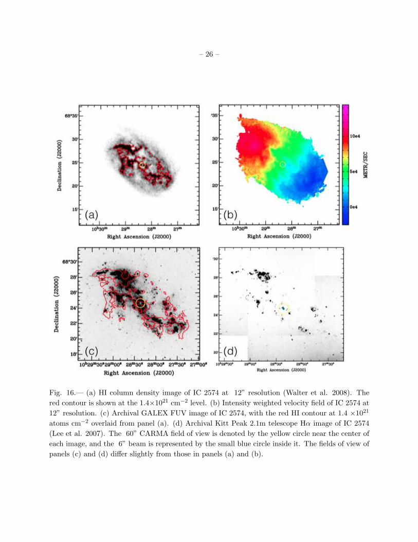
IC 2574 (see Figure 16) is a very famous example of a fairly low-mass, metal poor galaxy, withover 370 references to it in the NASA Extragalactic Database. It has a metallicity of 12+log(O/H)≈ 8.15 (≈ 30% Z Miller & Hodge 1996), and an HI mass of 1.4 ×109 M (Walter & Brinks1999) at an adopted distance of 3.94 Mpc (Melbourne et al. 2012). This galaxy is particularlyinteresting because of the structure in its HI gas distribution, which reveals 48 holes ranging insize from 100 pc to 1000 pc (Walter & Brinks 1999). These features are likely to form when anepisode of vigorous star formation produces young massive stars whose stellar winds and type IIsupernovae provide enough mechanical energy to drive away gas and sometimes trigger secondarystar formation on the edges of the newly-formed shells. The largest (supergiant) shell in IC 2574provides a textbook example of triggered star formation around an HI shell (Weisz et al. 2009).Shells are most easily studied in dwarf galaxies because dwarfs undergo solid body rotation; thelack of shear in the disk allows structures to persist for longer than in disk galaxies.

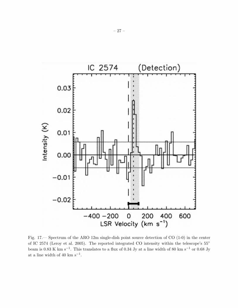
Star formation relies on the presence of molecular gas, but molecular gas clouds had not previouslybeen studied in detail in this galaxy. A single pointed observation with the ARO Kitt Peak 12mtelescope (Leroy et al. 2005) reports a point-source detection of CO (1-0) in the galaxy’s centerwith an intensity of ICO = 0.83 K km s−1 over a beam area of 55” (see Figure 17 for the detectionspectrum). A follow-up observation by the IRAM 30m telescope in CO (2-1), however, reports anon-detection (Leroy et al. 2009). This interesting discrepancy means that the gas cloud or cloudsat the ARO 12m pointing are probably very dense, causing the molecular component to remainvery cool and preventing strong emission from higher-energy transitions. We therefore carry out amore detailed study of the molecular gas in IC 1574 at 115 GHz with CARMA, the first attemptat such an observation with an interferometer.

– 25 –

6.2. Observations and Results

We observed the center of IC 2574 for a total time of ≈10 hours. The 60” CARMA15 field ofview completely covered the ≈55” ARO 12m telecope’s beam. Our correlator setup achieved avelocity resolution of 0.6 km s−1 in the range -20 km s−1 to 140 km s−1, covering the entire velocityrange where CO emission was found in the previous detection. Our two observing tracks, bothtaken in the late morning to early afternoon, gave us a combined on-source time of ≈10 hours.Unfortunately, the data was compromised by bad weather: one track received a weather grade ofC and the other a grade of D. The CO emission line was affected the most strongly, as it is foundnear to the 118 GHz oxygen line.

Standard reduction techniques were performed on the data using the MIRIAD software package.Our final unaveraged data cube displayed an RMS noise level of 248 mJy beam−1 at a line widthof 62 MHz and a beam size of 7.28” × 6.66”. This is over six times noisier than predicted by theCARMA sensitivity calculator, which expected a noise level of 42.9 mJy beam−1 at the same linewidth under normal weather conditions. We attribute this discrepancy to the bad weather. Wealso created data cubes with channels averaged to 2, 5, 10, 20, 40, 60, and 80 km s−1 velocityresolution. We do not detect significant CO emission from the galaxy in any of our cubes.

6.3. Discussion and Conclusions

The Leroy et al. (2005) CO (1-0) detection reports an intensity of ICO = 0.86 ± 0.17 K km s−1,or 27.3 Jy km s−1. Their spectral line width is published only graphically, but we estimate it tobe at most 80 km s−1. This translates to a flux of 341 mJy across a 55” beam. If we average ourchannels to a velocity resolution of 20 km s−1 to better compare with the Leroy et al. spectrum,our RMS noise becomes 35.9 mJy. Despite the bad weather, these numbers suggest that if thesource were a single point source it should have been detected. It is therefore likely that the Leroyet al. ≈55” beam actually covers more than one cloud of molecular gas hiding just below ourcurrent noise threshold. This prediction is supported by the distribution of Hα, a tracer of ongoingstar formation, in Figure 16d. The image shows multiple knots of star formation within CARMA’s≈60” field of view at our pointing, and since molecular gas is associated with star forming regions,it is likely that the CO emission would appear as multiple point sources as well.

To conclude, due to bad weather we did not confirm the detection of CO in the famous metal-deficient dwarf galaxy IC 2574, previously detected by the Kitt Peak ARO 12m single dish telescope.Comparing our RMS noise threshold with the intensity of the CO emission found by the previousdetection, we conclude that if the molecular gas in IC 2574 were a point source to our ≈7” beam,we would have detected it. We interpret this finding, coupled with the Hα detection of multiplestar forming regions within the ARO 12m telescope’s beam, as evidence that the molecular gas inIC 2574 is extended over a large area, making it difficult to detect with CARMA’s higher spatialresolution.

– 26 –

Fig. 16.— (a) HI column density image of IC 2574 at 12” resolution (Walter et al. 2008). Thered contour is shown at the 1.4×1021 cm−2 level. (b) Intensity weighted velocity field of IC 2574 at12” resolution. (c) Archival GALEX FUV image of IC 2574, with the red HI contour at 1.4 ×1021

atoms cm−2 overlaid from panel (a). (d) Archival Kitt Peak 2.1m telescope Hα image of IC 2574(Lee et al. 2007). The 60” CARMA field of view is denoted by the yellow circle near the center ofeach image, and the 6” beam is represented by the small blue circle inside it. The fields of view ofpanels (c) and (d) differ slightly from those in panels (a) and (b).

– 27 –

Fig. 17.— Spectrum of the ARO 12m single-dish point source detection of CO (1-0) in the centerof IC 2574 (Leroy et al. 2005). The reported integrated CO intensity within the telescope’s 55”beam is 0.83 K km s−1. This translates to a flux of 0.34 Jy at a line width of 80 km s−1 or 0.68 Jyat a line width of 40 km s−1.

– 28 –

7. Sunyaev-Zel’dovich Observations of the ZW3146 Galaxy ClusterJonathan Florez (Fisk University) and Devin Crichton (Johns Hopkins University)

7.1. Introduction

In the past couple of decades the quality of Sunyaev-Zel’dovich Effect (SZE) observations haveincreased drastically due to the development of radio interferometers that have improved low-noise detectors and systematics. Such instrumental developments have allowed us to study thehot intracluster medium (ICM) gas of galaxy clusters, ranging in mass from 1014–1015 M, acrossa wide spectrum of angular scales (Carlstrom et al. 2002). The SZE produces inverse Comptonscattering of CMB photons on the hot electron gas of the ICM, making it a useful tool in the studyof the massive galaxy clusters and their baryonic content. Current observations of galaxy clustershave shown that a great deal of clusters in similar mass ranges have a hot ICM gas that emitsX-rays (De Lucia et al. 2004). As a result, SZE and X-ray observations complement each othervery well and give us multiple ways to probe the ICM gas of massive clusters. A detailed study ofcombined SZE and X-ray data will allow us to better understand certain physical processes drivingthe evolution of such massive clusters (Zhang & Wu 2000).

Our target for the CARMA 2014 Summer School was ZW3146, a galaxy cluster at z = 0.291that has high X-ray emission (Mushotzky & Loewenstein 1997) and is massive enough to produceflux decrements in the CMB map at 30 GHz. These flux decrements, due to the SZE, becamevisible after ∼10 hours of observations and required detailed reduction and faulty data flagging.We collected ∼17 hours of observations at 30 GHz using the Sunyaev-Zel’dovich Array (SZA) atCARMA and acquired a significant detection after modeling and removing two point sources fromthe field of view. SZE observations of ZW3146 combined with existing X-ray and lensing datawill allow us to better understand the three-dimensional structure of the dark matter halo of thiscluster and the physics of its ICM.

In this report we provide a brief introduction to the SZE, describe our observations of the SZEof ZW3146 during the CARMA Summer School 2014, detail the data reduction methodologies weused on the data thus acquired and conclude with an description of the results.

7.2. Sunyaev-Zel’dovich Observations of Galaxy Clusters

The relic thermal radiation from the big bang, which we observe today as the cosmic microwavebackground (CMB), provides a useful backlight that we can leverage to probe the intervening struc-tures in the universe. The Sunyaev-Zel’dovich Effect (SZE, Sunyaev & Zeldovich 1980) refers tothe inverse Compton scattering of the CMB photons by hot plasmas such as the gravitationallyshock-heated gas residing in the dark matter halos of galaxy groups and clusters as shown schemat-ically in Figure 18. This imprints a characteristic spectral distortion on the thermal spectrum ofthe primordial CMB signal. The lower energy CMB photons passing through such a pocket of hot

– 29 –

plasma have a small (. 1%) chance of being up-scattered to higher energies by interactions withthe more energetic ions. When we measure the microwave sky in the direction of these structures,we observe a decrement in the CMB signal at frequencies below ∼ 220 GHz and a correspondingincrement at higher frequencies.

0 100 200 300 400 500 600

ν[GHz]

ICMB

ICMB+SZ

∆I/ICMB

Fig. 18.— Left : A schematic diagram demonstrating the origin of the SZ effect; Low energy photonsfrom the CMB are scattered to higher energy through inverse Compton scattering with the hot ionsin the intracluster medium. Right : The spectral signature of the SZ effect. The dashed and dottedlines show, in flux density units, the blackbody CMB spectrum with and without a distortion fromthe SZ effect, respectively. The solid line shows the relative difference between these spectra andreflects the effective spectrum of the SZ effect as observed.

The SZ signal is thus observed as a frequency dependent distortion of the CMB intensity:

∆IνICMB

= y g(ν); y =σT

mec2

∫neTedl (1)

g(x(ν)) =x4ex

(ex − 1)2

(xex + 1ex − 1

− 4). (2)

Here, y is known as the Compton parameter and is proportional to the integral of the electronnumber density, ne, multiplied by the electron temperature, Te, along the line of sight. Thisquantity is therefore a measure of the integrated thermal pressure of ionized gas along a givendirection in the sky. In the non-relativistic limit, the spectral distortion function, g(ν), dependsonly on the dimensionless frequency, x ≡ hν/kBTCMB. The shape of this distortion is shown inFigure 18.

Massive clusters have y & 10−4 and, with ICMB ≡ 2(kBTCMB)3/(hc)2 = 270 MJy/sr and g(ν =30 GHz) ≈ −0.5 we expect to see a decrement signal on the order of 1 mJy/arcmin2. This in turnshould produce a signal of a few mJy/beam given the ∼ 100′′ beam of the compact subarray ofCARMA-8. This signal should be extended on the > 1′ angular scales typical of a cluster.

– 30 –

An important characteristic of the SZE is that, since it is a scattering process, the surface brightnessof the signal does not suffer from the same cosmological dimming with distance that is seen inemission processes. This makes the SZE a useful tool for probing the distant universe. Furthermore,the integrated SZ signal attributed to a cluster is related to the total thermal pressure of the ICM gasthat it hosts. Under the assumption of hydrostatic equilibrium the integrated SZ effect of a clusteris therefore expected to be a good proxy for its mass (Motl et al. 2005). The SZE may thereforebe used to trace the growth of structure in the universe over cosmological time scales, providingconstraints on cosmological parameters such as the amplitude of the matter power spectrum, σ8,and the fraction of the critical density of the universe attributed to matter, ΩM. However, inpractice, our ignorance of the details of the distribution of thermal pressure within galaxy clustersas well as deviations from hydrostatic equilibrium in the ICM systematically limit such studies(e.g., Hasselfield et al. 2013). Finer observations of the SZE over a wide range in angular scalessuch as those provided by interferometers are therefore crucial in enhancing precision cosmologywith the SZE.

7.3. CARMA-8 Observations of ZW3146 at 30 GHz

For our observations, we used the CARMA-8 (SZA) mode of the array, utilizing the 3.5m telescopesfor continuum observations at 1cm. For this purpose, the correlator was setup in the wideband modeand observations were scheduled for a single on target pointing with no mosaicing. In each cyclewe alternated between integrating for 15 minutes on our target and 3 minutes on our calibrationsource, 1058+015. As this is a >5 Jy source, it was used as both as a gain and passband calibrator.For flux calibration we observed Mars at the end of each of our observing runs which took placefrom 8/5/2014–8/9/2014. During this time ZW3146 was transiting at roughly 2PM local time,with a total up time of approximately 7 hours. Due to inclement weather on 8/5/2014, we havenot used the data taken on that day in this study. A summary of the observations used for thisproject is shown in Table 1. The total on target integration time in the raw data is ∼17 hours.

Table 1: Summary of observations carried out during the summer school.Observation Quality Grade Source integration Sky RMS τ230

Date time [hours] range [µm] range

8/6 A+ 3.74 500–800 0.5–0.88/7 A+ 3.16 500–1500 0.5–0.88/8 A+ 5.14 200–800 0.4–0.68/9 A+ 4.71 200–1000 0.4–0.8

After acquiring the data, we independently flagged each day’s visibility datasets, primarily focusingon spurious signals in some correlator windows and periods of system temperature or sky RMS

– 31 –

spikes. We used John Carpenter’s scripts1 to facilitate this process. The flagged and calibrateddata were then combined using the uvcat tool and clean images from the full dataset were producedusing the mossdi routine. The final clean and dirty maps are shown in Figure 19

Fig. 19.— Dirty (left) and clean (right) images of ZW3146 using all the data acquired during thesummer school, after flagging.

7.4. Point Source Subtraction

Within the observed field of view of the cluster lie two radio galaxies identified in the NVSS (NRAOVLA Sky Survey) at 1.4 GHz (Condon et al. 1998) and previously observed in 30 GHz studies ofthis cluster (Coble et al. 2007). Radio galaxies such as these appear as point sources in our data(Figure 20) and emit at 30 GHz, acting to fill in the expected decrement signal of ZW3146. Sincethis reduces the significance of the SZE detection and distorts the shape of the SZE signal, wemodeled the sources present in our data and subtract them from our reduced dataset.

We use the Difmap package, a program developed for the synthesis imaging of data from radiointerferometer arrays (Taylor 1997), to model the point sources in our field of view. Difmap offersunique mapping and interactive processing techniques that allow one to view and model the dataat different angular scales. In Difmap, one can load the visibility data and specify which baselinesto work with. The first step to modeling the point source in Difmap is to make a uvf file from thecombined reduced miriad data extracting only ZW3146 as the object of interest. The next step is

1http://carma.astro.umd.edu/carma/summerschool/2014/carma_calibrate.csh

– 32 –

Fig. 20.— Locations of NVSS point sources in the field overlayed with signal to noise contours ofthe reduced CARMA-8 data which has been cut to display only the long baselines to the out-riggerantennas 18 and 19. The optical image is derived from optical SDSS observations of ZW3146 inthe i, r and g bands.

to load the long baseline visibility data into Difmap to get a view of the residual map. A 4.2 mJysource is strongly visible at roughly 100 arcseconds from the target center. A second, less noticeablepoint source is located slightly southeast of the image center and exhibits a flux of roughly 2 mJy.Using a command in Difmap known as ‘modelfit’ one can model point sources and subtract themfrom the long baselines. After subtracting the point sources from the field of view we are left withwhat looks like noise in the residual map. The long baseline map before and after the subtractioncan be seen in Figure 21.

7.5. Results and Conclusions

We present our map of cluster ZW3146 in Figure 22 after the point sources have been subtractedin the long baselines. Once again we use Difmap to read in the short baseline visibility data. Thecluster clearly exhibits a flux decrement near the center of the map, at -4 mJy/beam. The clustersignal of the SZE appears roughly 100 arcseconds in diameter, with the peak slightly off center.The flux decrement exhibited by the cluster only becomes significant after ZW3146 acquires over10 hours of integration time.

We observed ZW3146 for 17 hours to get the result we present in this memo. We find that in orderto acquire any good visibility data we must flag out any bad channels and antennas, as well asthrowing out any data that may have been acquired during bad weather. Point source subtraction

– 33 –

(a) Long baseline data before point source subtraction (b) Long baseline data after point source is removed

Fig. 21.— The long baseline visibility data displayed in Difmap. A point source can be seen inthe first map, at ∼ 100 arcseconds to the left of the image center. Another point source, slightlyharder to detect, is noticeable also ∼100 arcseconds southeast of the map center. After modelingthe point sources and removing them we get the resulting residual map on the right which lookslike noise, i.e. there are no other sources apparent.

is also an important part of the process prior to viewing the full SZ signal, as flux from the pointsources can interfere with the short baseline visibility data. The resulting data is a uvf file thatcan be used to acquire important information about the cluster, such as its characteristic physicalscale, R500 and Compton-y parameters, which can in turn teach us about the physics of the hotICM gas.

– 34 –

Fig. 22.— The short baseline visibility data after the point sources in the field of view have beensubtracted.

– 35 –

8. CO Observations of the Host Galaxy of Broad-lined Type SN Ic 2005ksPatrick Kelly (University of California, Berkeley)

8.1. Introduction

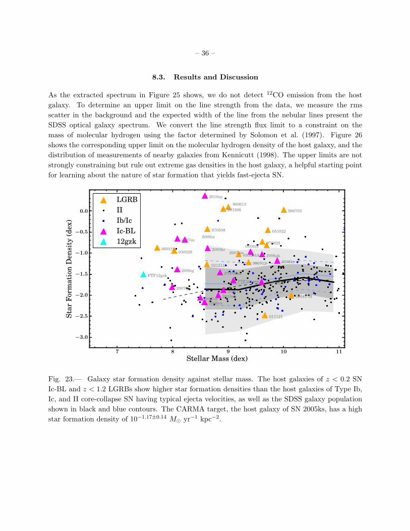
The supernovae (SN) associated with long-duration gamma-ray bursts (LGRBs) are broad-linedType Ic (Ic-BL) explosions, whose spectra exhibit wide features consistent with ejecta velocitiesof ∼0.1c. In a recent paper Kelly et al. (2014), we showed that the host galaxies of SN Ic-BLand LGRBs have high stellar-mass and star-formation densities, in comparison to SDSS galaxiesthat have similar stellar masses (see Figure 23). Core-collapse SN having typical ejecta velocities,however, do not exhibit any preference for overdense galaxies. This suggests that star formationmust proceed differently in the overdense host galaxies of SN Ic-BL and LGRBs.

My CARMA summer school project was to measure or constrain the molecular hydrogen contentof the host galaxy of SN 2005ks, a nearby z = 0.098 broad-lined SN Ic. This measurement is anecessary step (along with HI host galaxy measurements) to being able to determine whether starformation is consistent with the Kennicutt-Schmidt relation between star-formation density andgas density Kennicutt (1998); Schmidt (1959). Given the ability to detect LGRBs at high redshift,they may become important tracers of star formation in low-luminosity galaxies too faint to bedetected even by e.g., Giant Magellan Telescope, and the Thirty Meter Telescope.

A color composite image of the z = 0.098 host galaxy shown in Figure 24. The star-formationdensity of the host galaxy of SN 2005ks is 10−1.17±0.14 M yr−1 kpc−2.

8.2. Observations and Data Reduction

We obtained a 5.7 hr integration centered on the host galaxy coordinates α =21:37:56.52 andδ =-00:01:57.64 in the CARMA 15-antenna compact E configuration in favorable atmospheric con-ditions. During the track, τ ≈ 0.81 and the phase rms was 205 µm. We observed the 12CO(1 -0) emission line at 115.27 GHz. From the spectroscopic galaxy redshift available from the SDSSsurvey2, we calculated that this transition has an observer frame frequency of 104.92 GHz. We con-figured the correlator to bracket this frequencey with a 250 MHz band, and placed seven additional250 MHz bands adjacent in frequency to this center band.

The data were reduced using the sequence of steps in the MIRIAD script provided by John Car-penter. Several attennas were not functioning properly and were removed, but the data requiredminimal flagging. We extracted a spectrum within a 5′′ square aperture positioned at field centerthat contains the host galaxy optical emission.

2http://skyserver.sdss3.org/public/en/get/SpecById.ashx?id=4723347288133992448

– 36 –

8.3. Results and Discussion

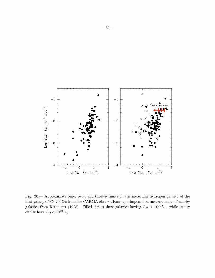
As the extracted spectrum in Figure 25 shows, we do not detect 12CO emission from the hostgalaxy. To determine an upper limit on the line strength from the data, we measure the rmsscatter in the background and the expected width of the line from the nebular lines present theSDSS optical galaxy spectrum. We convert the line strength flux limit to a constraint on themass of molecular hydrogen using the factor determined by Solomon et al. (1997). Figure 26shows the corresponding upper limit on the molecular hydrogen density of the host galaxy, and thedistribution of measurements of nearby galaxies from Kennicutt (1998). The upper limits are notstrongly constraining but rule out extreme gas densities in the host galaxy, a helpful starting pointfor learning about the nature of star formation that yields fast-ejecta SN.

7 8 9 10 11

Stellar Mass (dex)

−3.0

−2.5

−2.0

−1.5

−1.0

−0.5

0.0

Star

Form

atio

nD

ensi

ty(d

ex)

LGRBIIIb/IcIc-BL12gzk

090417B

051022

991208980613

011121

990712

970828

980703

060218

970508

010921

021211

050416A030329

2010ay

2005ks

2007eb

PTF10aavz

2007I

2006aj

2006nx

2007bg

2005kr

2010ah

2006qk

2007ce

2007qw

2008iu

PTF09sk

PTF10qts

PTF12gzk

Fig. 23.— Galaxy star formation density against stellar mass. The host galaxies of z < 0.2 SNIc-BL and z < 1.2 LGRBs show higher star formation densities than the host galaxies of Type Ib,Ic, and II core-collapse SN having typical ejecta velocities, as well as the SDSS galaxy populationshown in black and blue contours. The CARMA target, the host galaxy of SN 2005ks, has a highstar formation density of 10−1.17±0.14 M yr−1 kpc−2.

– 37 –

Fig. 24.— SDSS color composite image of the target z = 0.098 host galaxy of SN 2005kz. Thered square shows the positions of the 3′′-diameter SDSS spectroscopic fiber. The host galaxy has asemi-major axis length of ∼5′′.

– 38 –

Fig. 25.— The extracted spectrum from a 5′′ square aperture positioned at field center enclosingthe host galaxy optical emission. The spectrum wavelength coverage corresponds to a window thatshould contain 12CO(1 - 0) emission in the host galaxy rest frame. No signal is detected, and wecompute an upper flux limit that we convert to a constraint on the molecular hydrogen gas density.

– 39 –

SN 2005ks Host

Fig. 26.— Approximate one-, two-, and three-σ limits on the molecular hydrogen density of thehost galaxy of SN 2005ks from the CARMA observations superimposed on measurements of nearbygalaxies from Kennicutt (1998). Filled circles show galaxies having LB > 1010L, while emptycircles have LB < 1010L.

– 40 –

9. 1 mm Observation of M6III Red Giant Star g HerLauren McKeown (Trinity College, Dublin)

9.1. Scientific Motivation

g Her is a semi-regular pulsating red giant star. It is particularly interesting because it has a spectraltype similar to where dust first appears. All cool stars possess atmospheres heated to temperaturesabove that predicted by the classical assumption of Radiative Equilibrium (Schrijver & Zwaan2000). This is due to convective motions beneath the photosphere agitating the local plasma andresulting in magnetic and acoustic disturbances, hence initiating non-radiative heating of the upperphotosphere, resulting in a chromosphere. The heated plasma has a chromospheric spectrum inthe UV which has been studied at length with spectrographs on IUE and HST (McMurry 1999).There exist two schools of thought on the physical structure of quiet chromospheres. The firstargues that spectral signatures indicate a persistent outward temperature rise (Kalkofen et al.1999), thought to be magnetic in origin. The second involves a time-variable plasma which ispurely acoustically-shocked, where at a given position the gas temperature would fluctuate fromvery hot to very cool, with the mean temperature being cool (Wedemeyer-Bohm et al. 2007). Thiswould not produce a persistent chromosphere. UV observations alone cannot determine the heatingmechanism associated with these chromospheres, as persistent chromospheres and intermittently-shocked plasmas can share similar time-averaged UV emission owing to their high temperature fluxsensitivity ∼ 〈e−

hνkT 〉 when hν > kT .

Fortunately, these heated plasmas also have thermal continuum signatures at mm wavelengths(Altenhoff et al. 1994; Loukitcheva et al. 2004) where the source function is a linear function oftemperature ∼ 〈T 〉. The intermittent and persistently formed chromosphere theories cannot satisfy

both the UV and mm constraints, i.e., 〈e−hνkT 〉 6= e

− hνk〈T 〉 . The mean temperature from the intermit-

tent chromospheric model does not increase outwards like that anticipated from magnetic heatingand this can be detected at mm wavelengths. Emission at a particular frequency originates froma range of atmospheric depths and hence multiple frequency observations from CARMA can infergas temperature gradients to differentiate between the two competing models for chromospherictemperature gradients.

g Her has been observed at 1 mm by (Harper et al. 2013) using CARMA D config and by (Altenhoffet al. 1994) using the IRAM 30 m telescope. Altenhoff et al. obtained an upper limit on the fluxof g Her at 250 GHz of < 6 mJy with a corresponding spectral index of < 1.0. The red giant hasalso been observed by Harper et al. at 3 mm with the aim of using the flux density inferred atboth wavelengths in order to determine the mm spectral index of g Her. The original observationmade at 1 mm by (Harper et al. 2013) was unfortunately affected by bad weather and so follow-upcontinuum observations of g Her at 1 mm will allow us to determine the spectral index of g Herand hence further understand the chromospheric temperature structure of this object.

– 41 –

9.2. Observations and Data Reduction

g Her was observed using CARMA for over 2 hours at a rest frequency of 225 GHz. The 15-element array of 6.1 and 10.4 m antennas was in E-configuration, with baselines ranging between8.5 m and 66 m. As this was a point-source observation, we did not mosaic our map of g Her.Mars was used as a flux calibrator, while 3C345 was observed intermittently between observingour target as a phase calibrator. 3C345 was also used as a passband calibrator. The data wascalibrated using the package MIRIAD (Sault et al. 1995) Next, shadowed antennas were flagged.Data inspection indicated that antennas 7, 10, 12 and 14 required flagging for a ∼ 2 min timerange. Close monitoring during observations led us to source antenna collision as one of the causesfor bad data during this time frame.

Our 1 mm image of g Her was produced using the MIRIAD invert task. To create the final map,the original map of g Her was cleaned using the clean task and convolved with the synthesizedbeam using restor. Imfit was used to fit an elliptical 2D Gaussian to our map, giving us a value forthe peak flux and integrated flux from our target at 1 mm.

(a) 1mm radio map of g Her (b) 1 mm contour map of g Her

Fig. 27.— Results of CARMA 15-element array 1 mm observations of g Her

9.3. Results

The map obtained from our observations of g Her indicated a peak flux density of 21.1 ± 2.4mJy with a noise level of 4 mJy/beam. Considering g Her is a faint source, we were still able to

– 42 –

identify our target at the centre of our clean map. Applying a 2D Gaussian fit to our map gave apeak flux of 18.9 ± 3.6 mJy and an integrated flux of 35 mJy. Having inspected that the box sizewas sufficient to surround our target and no neighboring outliers, the significant difference in peakand integrated flux density derived from applying a 2D Gaussian to our source may indicate theexistence of another mm source behind our target, or contamination from background noise. Theresulting peak flux of 21.1 mJy was close to the semi-analytic model prediction of (Harper et al.2013) which was 24 mJy. We have used this flux and our CARMA 2012 observed 3mm flux to infera preliminary spectral index for g Her of 1.62. This differs greatly from the upper limit of < 1.0 setby Altenhoff et al. (1994). An explanation for this may be that the pulsating nature of g Her mayinduce considerable variability at mm wavelengths and hence, comparing fluxes at 1 mm and 3 mmtwo years apart in calculating spectral index may not be an accurate method for the requirementsof our study. We have proposed 1 mm and 3 mm follow-up observations of four red giant stars inour sample of six for CARMA semester 2014b, which includes g Her and which will allow us tofurther inspect whether g Her exhibits variability at these wavelengths. Combined, our CARMAobservations will provide deep insight into the chromospheric thermal structure of g Her, which hasnot yet been explored in such detail as we propose with CARMA.

This research has been conducted with the financial support of Science Foundation Ireland underGrant Number SFI11/RFP.1/AST/3064

– 43 –

10. Tracing Outflows from Per-8Erin Cox, Ko-Yun (Monica) Huang (UIUC), Dana Anderson (Caltech), & Maryam

Tabeshian (Univ. of Waterloo, Ontario)

10.1. Introduction

Perseus-8, also known as IRAS 03292+3039, is a dense core in the B1 region of the Perseus molecularcloud. This molecular cloud hosts low-mass pre-main-sequence stars, embedded protostars, andstarless cores within its total mass of 10,000 M and resides at a distance of 250±50 pc. Theclassification of Per-8 has changed over time, but Schnee et al. (2012) re-classified it as a Class 0protostar after observing its outflows in CO and C18O. By studying the outflows of these young(having ages of a few times 104 years) protostars, we can learn about the structure and dynamicsof their parent cloud and further our understanding of the star-formation process.

10.2. Observations

We observed the Per-8 using CARMA 3mm E-array configuration (6.1m and 10.4m antennae) on2014 August 06. The total tracking length of time is 5.2 hours, while the actual time for our sourceis around 3.5 hours. The overall weather grade for our observation was given as A-.

Considering the size of the primary beam and the region of our interest, we used a 3-point mosaicto image the target region. We observed N2H

+(93.174Hz), HCN(88.632Hz), HCO+(89.189Hz),H13CO+(86.754Hz), and CH3OH(96.741Hz) with a bandwidth of 31 MHz; and three 500 MHzcontinuum windows were set to trace the dust mass.

3C84, one of the CARMA top tier secondary calibrators, was chosen as our phase and passbandcalibrator. It is a strong radio source which is 11 deg away from our source on the sky. And Uranuswas adopted as our flux calibrator.

During the observation, we had been through one modification to our script for shortening theintegration time for our passband calibrator 3C84. Also, at the latter phase of the observation,antenna 8 once stopped working, but resumed observing after the cycling of the power.

10.3. Data Reduction

The data were reduced using John Carpenter’s calibration and image scripts for a three-pointmosaic treating the narrow and wide bands separately to detect both spectral lines and continuumemission. Data from the second integration were flagged due to the spread in passband amplitudespossibly due to a change in the passband solution after restarting the observing script. Emissionfrom the three wide bands was combined to produce the image of the continuum emission fromthe source. Spectral lines were identified in channel maps of the narrowband emission averaged

– 44 –

over 1 km s−1 intervals. Using the non-spectral channels in each narrow band, the level of thecontinuum emission was estimated and subtracted from the total emission. Images were cleanedto a cutoff of three times the level of the root-mean-square (RMS) noise. The figures shown inthe following section are the signal-to-noise maps of the combined wideband (continuum) emissionand the continuum-subtracted narrowband emission from the spectral lines. Spectra were createdfrom the narrowband emission over a 20 × 20 ” square centered on the highest point in the dustemission observed by Schnee et al. (2012).

10.4. Results

10.4.1. Continuum

The map of the continuum emission from our source is shown in Figure 28. The point of highestemission at the center is roughly in agreement with that observed by Schnee et al. (2012). (indicatedby the white star in Figure 28 and all subsequent maps).

10.4.2. N2H+

Figure 29 shows the outflow as seen inN2H+ emission. N2H

+ is known to be a tracer of dense gasand its bulk motion. The emission maps are sampling emission from the seven hyperfine componentsof the J = 1–0 transition of N2H

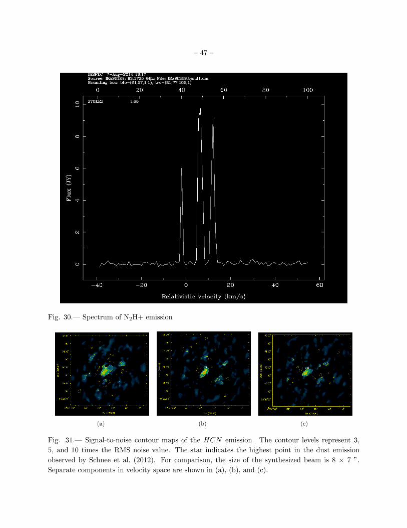
+. Not all of the hyperfine components were resolved as seen inthe spectrum provided in Figure 30.

10.4.3. HCN

HCN data is seen in Figures 31 and 32. There is evidence for an outflow seen in all three channelsof the HCN maps. This is in the direction that Schnee et al. (2012) found CO to be blue shifted.The flux seen in the three separate channels is due to the three hyperfine components in the HCNline. These are also seen in the spectrum seen in Figure 32. The central velocity of these linesmatches those that are found in Schnee et al. (2012).

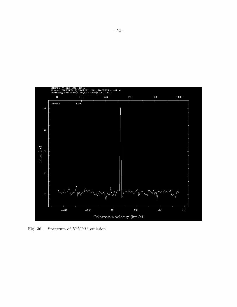
10.4.4. HCO+ and H13CO+

Maps and spectrum of HCO+ are seen in Figures 33 and 34. There is an obvious outflow structureseen, at least in the first image (blueshifted component), and a possible redshifted component.Figures 35 and 36 show the H13CO+ data. The map shows that the majority of the emission isseen close to the central part of the map.

– 45 –

Fig. 28.— Signal-to-noise contour map of the combined wideband emission. The contour levelsrepresent 3, 5, and 10 times the RMS noise value. The star indicates the highest point in the dustemission observed by Schnee et al. (2012). For comparison, the size of the synthesized beam is 8 ×7 ”.

– 46 –

(a)

(b)

(c)

Fig. 29.— Signal-to-noise contour maps of theN2H+ emission. The contour levels represent 3,

5, and 10 times the RMS noise value. The star indicates the highest point in the dust emissionobserved by Schnee et al. (2012). For comparison, the size of the synthesized beam is 8 × 7 ”.Separate components in velocity space are shown in (a), (b), and (c).

– 47 –

Fig. 30.— Spectrum of N2H+ emission

(a) (b) (c)

Fig. 31.— Signal-to-noise contour maps of the HCN emission. The contour levels represent 3,5, and 10 times the RMS noise value. The star indicates the highest point in the dust emissionobserved by Schnee et al. (2012). For comparison, the size of the synthesized beam is 8 × 7 ”.Separate components in velocity space are shown in (a), (b), and (c).

– 48 –

Fig. 32.— Spectrum of HCN emission. The three hyperfine components are resolved.

– 49 –

10.5. Discussion

Dust emission observed in the continuum was found to have a central point near where Schneeet al. (2012) found the point of highest dust emission. We found detections of all molecules weobserved, except CH3OH, which was not expected to be seen. The resolution of the array wasnot good enough to resolve all seven hyperfine components of the N2H

+ line, but three peaks wereseen, with their velocity centers consistent with what Schnee et al. (2012) measured. We were ableto resolve all three of the hyperfine components in HCN , again having consistent central velocities.

We found evidence for outflows in both HCN and HCO+. Both maps have a blue shifted com-ponent of an outflow, and the HCO+ maps show signs for a possible redshifted component aswell. Though, given the level of contours seen, we cannot say if there definitely is. In N2H

+ and inH13CO+ we see the largest flux near the center of the field, close to where the largest dust emissionis coming from. While all of these molecules trace bulk motion, N2H

+ tracks the densest material,so it makes sense that outflows are not seen using it. The definite outflow structure seen in HCO+

is an exciting result. This is because, while it’s predicted to be a large part of protostars, it hasnot been detected very many times.

We hope to analyze this data using different techniques, such as moment maps or PV diagrams,to get a better constraint of where the gas really is. This can help narrow down what processesare really happening, and where. For future work, it would be ideal to also observe CO isotopesand the polarization of the dust grains. This will again give a broader view of what is actuallyhappening in near the protostar.

– 50 –

(a) (b)

Fig. 33.— Signal-to-noise contour maps of the HCO+ emission. The contour levels represent 3,5, and 10 times the RMS noise value. The star indicates the highest point in the dust emissionobserved by Schnee et al. (2012). For comparison, the size of the synthesized beam is 8 × 7 ”. Theseare not separate velocity components, the different maps are a consequence for how the channelswere binned.

– 51 –

Fig. 34.— Spectrum of HCO+ emission.

(a)

Fig. 35.— Signal-to-noise contour maps of the H13CO+ emission. The contour levels represent 3,5, and 10 times the RMS noise value. The star indicates the highest point in the dust emissionobserved by Schnee et al. (2012). For comparison, the size of the synthesized beam is 8 × 7 ”.

– 52 –

Fig. 36.— Spectrum of H13CO+ emission.

– 53 –

11. Observing a massive galaxy cluster at medium redshiftJay Franck (Case Western Reserve), Andrew Nadolski (UIUC), Bandon Decker

(Univ. Missouri, Kansas City)

11.1. Background

Galaxy clusters are the largest gravitationally bound objects in the universe; as such, they makeexcellent cosmological probes. The majority of the baryonic mass of a galaxy cluster is in theform of an electron plasma known as the intracluster medium (ICM). This gas emits thermallyin the X-ray, but it also inversely Compton scatters the cosmic microwave background radiation(CMB)Sunyaev & Zeldovich (1975). For the frequencies at which we looked, this effect manifestsas a decrement appears in the otherwise uniform CMB. This is the Sunyaev-Zel’Dovich effect; themagnitude of the decrement is related to the density of the ICM along the line of sight which is inturn related to the mass of the clusterAndersson et al. (2011). The SZ effect is largely independentof redshift, making it an excellent tool for measuring the mass of distant galaxy clusters.

11.2. Observation

To fulfill the goals outlined for CARMA Summer School 2014, it was of paramount importanceto observe an object that is known to have an easily identifiable signal. For this reason, wechose MACSJ0717.5+3745 as it is an incredibly massive cluster with an estimated mass of M(r <1Mpc) > 2× 1015M at a redshift of z = 0.55 Limousin et al. (2012). When considering potentialweather issues, the need for a structure that could be detected by the SZ effect in a minimumamount of time was important. Clusters in the high redshift regime (especially at z ≥ 1 requirelarger time commitments Muchovej et al. (2007); Culverhouse et al. (2010), even upwards of 50hours of on source time Mantz et al. (2014).

We began observations on August 5, 2014 at 04:43 LST. Our track time totaled 5.2 hours, 3.8 ofwhich were spent on source. The remaining time was devoted to phase calibration using J0646+448.We were unable to observe a flux calibrator. We conducted observations at 30Ghz using the SZAantennae. Weather conditions were generally poor. Sky RMS was consistently 1000 microns orgreater and τ230 ranged from 0.57 to 2.71. Consequently, a great deal of data flagging (includingcuts to time, system temperature, and baselines) was required to produce a clean map.

11.3. Results

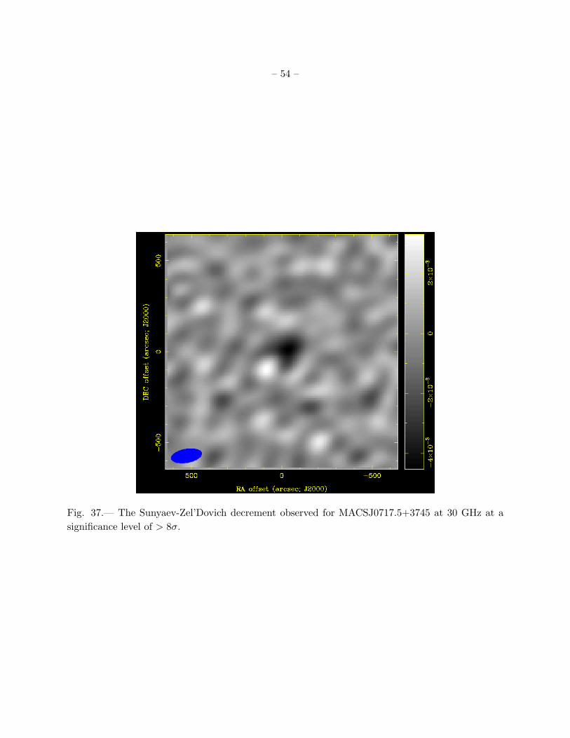
With a track length of only ∼ 5 hours, of which 3.4 hours was on source, we were able to detectan SZ decrement from MACSJ0717.5+3745 (pointed at RA 07:17:31.7 and DEC +37:45:18.2) at asignificance level of > 8σ from the RMS noise. Figure 37 shows the clean map of the cluster’s SZeffect. Based on the relatively small track time used, these authors recommend this cluster for the

– 54 –

Fig. 37.— The Sunyaev-Zel’Dovich decrement observed for MACSJ0717.5+3745 at 30 GHz at asignificance level of > 8σ.

– 55 –

target of future CARMA Summer School projects.

– 56 –

12. Observations of 12CO and 13CO in Molecular Outflow L1228 AAmy Steele (University of Maryland) and Ned Molter (Macalester College)

12.1. Introduction

Molecular outflows are a type of mass-loss phenomena associated with the earliest stages of stellarevolution. Emission maps of molecular flows reveal cloud structure and provide insight on theinitial conditions of the star formation process. Additionally, the flows constrain models of cloudcollapse and star formation, since the flow momentum leaves a fossil record of the mass loss historyof the centrally embedded protostar (Bally et al. 1995).

We observed a warm, compact source as well as 12CO and 13CO in the molecular outflow of theL1228 cloud. L1228 is located at ∼ 200 pc and is part of the Cepheus flare, a giant molecular cloudcomplex in Cepheus, which is also part of the Gould’s Belt system (Bally et al. 1995). The cloudspans 0.086 square degrees and has a vLSR = −7.6 km/s (Bally et al. 1995). L1228 consists of threecenters of star formation (Kun et al. 2008), one of those being the L1228 core, or L1228 A. Wefocus on L1228 A in this memo (α: 20:57:13, δ: 77:35:44), as it contains the Class I source IRAS20582+7724, which is driving the outflow.

Millimeter wavelength observations of the region reveal continuum emission from warm dust sur-rounding the young star as well as red- and blueshifted bipolar outflows showing bulk motions.

12.2. Observations

We observed L1228 for 3.1 hours on August 6, 2014 using the CARMA-15 array in its compact Econfiguration with baselines ranging from 8.5 m to 66 m. The flux was calibrated at the beginningof the track using Neptune. Quasar 3C454.3 was also observed once at the beginning of the track tocalibrate the bandpass by measuring channel-to-channel variations of the correlator. Observationsof the point-like source 1927+739 were interleaved with the science target to follow the behaviorof the atmosphere and instrumental phase during the track. The overall grade for the track was a‘B’ since the sky phase RMS was ∼ 346µm, and τ hovered around 1.8. The correlator was setupsuch that the LO frequency was 108 GHz with the continuum source observed in five 500 MHzwindows in the upper and lower sidebands. The lower sideband was also configured to potentiallyobserve C18O, 13CO, and 12CO in narrowband 31 MHz windows. Additionally, we only observedLL polarization, even though CARMA is capable of observing 4: LL, RR, LR, RL.

– 57 –

12.3. Data Reduction

The resulting data was calibrated using MIRIAD software3, and initially inspected using John Car-penter’s data reduction script. After inspecting the data, we found that no flagging was necessary.We then wrote a script that would calibrate the data from this specific observation. The passband,flux, and gain were calibrated using the mfcal, bootflux, and mselfcal routines. After calculat-ing the gain, it was applied to the narrowband CO data. The routine mselfcal was run on thephase calibrator to find the offset between the narrow- and widebands. After calibration, we tookthe Fourier transform of the sky distribution (invert), ran a CLEAN alorithm (clean), and thenre-convolved the cleaned components with the beam (restor). Maps of the distribution of CO andthe continuum source are provided in figures 1-4.

12.4. Results

We detected 12CO, 13CO, and a contiuum source (see figure 40) toward L1228. The CO emissionis overall spatially aligned with the compact contiuum source. Based on line velocity maps of theCO isotopes, we did not detect 18CO. Integrated intensity maps of the zeroth moment show thatthe 12CO is extended in the east-west direction (see figure 38). The emission in the east direction isblueshifted, while the emission in the west direction is redshifted. The maps of the 13CO also showsome bulk motion (see figure 39), though not as spatially extended as the 12CO. The radial velocityof the source is reflected in the central line velocity of the CO emission lines (see figure 42). The12CO shows a double-peaked velocity structure indicative of bulk motion from the outflow centeredat the LSR velocity of L1228 A (−7.6 km/s). However, the 13CO shows a single peak centered nearthe system velocity, suggesting that this emission originates from a region close to the embeddedsource. These results are consistent with the 12CO and 13CO maps from Bally et al. 1995. A fullimage of the region is shown in figure 41.

3See http://www.cfa.harvard.edu/sma/miriad/.

– 58 –

Fig. 38.— Molecular outflow L1228 A. A map of 12CO with red contours at 3, 6, and 9 × RMS.Blueshifted emission is shown in solid blue, and redshifted emission is shown in red. Dashed linesshow negative contours. The size is the synthesized beam is shown with the blue hatched oval.

– 59 –

Fig. 39.— Molecular outflow L1228 A. A map of 13CO with red contours at 3, 6, and 9 × RMS.Blueshifted emission is shown in solid blue, and redshifted emission is shown in red. Dashed linesshow negative contours. The size is the synthesized beam is shown with the blue hatched oval.

– 60 –

Fig. 40.— Molecular outflow L1228 A. A map of the continuum at 0.3 cm with 0.04 Jy/beam.

– 61 –

Fig. 41.— Molecular outflow L1228 A. A map of 12CO (in blue), 13CO (in green), and 0.28 mmcontiuum (pixelated at the center). The contours for the 12CO and 13CO are at 3, 6, and 9 × RMS.

– 62 –

Fig. 42.— Spectra of the CO in the direction of L1228 A. Top: left, 12CO; right, 13CO. Bottom:the non-detection of 18CO.

– 63 –

E-mail addresses

Patrick Kelly (UCB), patrick.l.kelly@gmail.com

Lauranne Lanz (CIT), llanz@ipac.caltech.edu

Lauren McKeown (TCD), mckeowla@tcd.ie

Scott Barenfeld (CIT), scott.barenfeld@gmail.com

Devin Crichton (JHU), dcrichto@pha.jhu.edu

Jonathan Florez (Fisk), jflorez0206@gmail.com

Amy Steele (Wesleyan), amysteele08@gmail.com

Ned Molter (Macalester), emolter@macalester.edu

Joey Rodriguez (Vanderbilt), rodriguez.jr.joey@gmail.com

Bandon Decker (UMKC), bbdz86@mail.umkc.edu

Jay Franck (CWRU), jrf110@case.edu

Shravan Avadhuta (CSU-LA), savadhu@calstatela.edu

Maryam Tabeshian (UWO), mtabeshi@uwo.cal

Dana Anderson (CIT), deanders@caltech.edu

Ko-Yun Huang (UIUC), khuang33@illinois.edu

Erin Cox (UIUC), egcox2@illinois.edu

REFERENCES

Alatalo, K., et al. 2013, MNRAS, 432, 1796

Altenhoff, W. J., Thum, C., & Wendker, H. J. 1994, A&A, 281, 161

Andersson, K., et al. 2011, ApJ, 738, 48

Bally, J., Devine, D., Fesen, R. A., & Lane, A. P. 1995, ApJ, 454, 345

Beasley, A. J., Gordon, D., Peck, A. B., Petrov, L., MacMillan, D. S., Fomalont, E. B., & Ma, C.2002, ApJS, 141, 13

Bigiel, F., Leroy, A., Walter, F., Brinks, E., de Blok, W. J. G., Madore, B., & Thornley, M. D.2008, AJ, 136, 2846

Cabrit, S., Pety, J., Pesenti, N., & Dougados, C. 2006, A&A, 452, 897

Cappellari, M., et al. 2011, MNRAS, 413, 813

Carlstrom, J. E., Holder, G. P., & Reese, E. D. 2002, arXiv preprint astro-ph/0208192

Coble, K., et al. 2007, AJ, 134, 897

Condon, J. J., Cotton, W. D., Greisen, E. W., Yin, Q. F., Perley, R. A., Taylor, G. B., & Broderick,J. J. 1998, AJ, 115, 1693

– 64 –

Culverhouse, T. L., et al. 2010, ApJ, 723, L78

De Lucia, G., Kauffmann, G., & White, S. D. 2004, Monthly Notices of the Royal AstronomicalSociety, 349, 1101

Fruscione, A., et al. 2006, in Society of Photo-Optical Instrumentation Engineers (SPIE) ConferenceSeries, Vol. 6270, Society of Photo-Optical Instrumentation Engineers (SPIE) ConferenceSeries

Guillard, P., et al. 2012, ApJ, 747, 95

Harper, G. M., O’Riain, N., & Ayres, T. R. 2013, MNRAS, 428, 2064

Hasselfield, M., et al. 2013, J. Cosmology Astropart. Phys., 7, 8

Kalkofen, W., Ulmschneider, P., & Avrett, E. H. 1999, ApJ, 521, L141

Kelly, P. L., Filippenko, A. V., Modjaz, M., & Kocevski, D. 2014, ApJ, 789, 23

Kennicutt, Jr., R. C. 1998, ApJ, 498, 541

Kun, M., Kiss, Z. T., & Balog, Z. 2008, Star Forming Regions in Cepheus, 136

Leroy, A., Bolatto, A. D., Simon, J. D., & Blitz, L. 2005, ApJ, 625, 763

Leroy, A. K., et al. 2009, AJ, 137, 4670

Limousin, M., et al. 2012, A&A, 544, A71

Loukitcheva, M., Solanki, S. K., Carlsson, M., & Stein, R. F. 2004, A&A, 419, 747

Mantz, A. B., et al. 2014, ArXiv e-prints

McMurry, A. D. 1999, MNRAS, 302, 37

Melbourne, J., et al. 2012, ApJ, 748, 47

Miller, B. W., & Hodge, P. 1996, ApJ, 458, 467

Motl, P. M., Hallman, E. J., Burns, J. O., & Norman, M. L. 2005, ApJ, 623, L63

Muchovej, S., et al. 2007, ApJ, 663, 708

Mushotzky, R., & Loewenstein, M. 1997, The Astrophysical Journal Letters, 481, L63

Ogle, P., Boulanger, F., Guillard, P., Evans, D. A., Antonucci, R., Appleton, P. N., Nesvadba, N.,& Leipski, C. 2010, ApJ, 724, 1193

Osterloh, M., & Beckwith, S. V. W. 1995, ApJ, 439, 288

– 65 –

Rodriguez, J. E., Pepper, J., Stassun, K. G., Siverd, R. J., Cargile, P., Beatty, T. G., & Gaudi,B. S. 2013, AJ, 146, 112

Roussel, H. 2013, PASP, 125, 1126

Sault, R. J., Teuben, P. J., & Wright, M. C. H. 1995, in Astronomical Society of the PacificConference Series, Vol. 77, Astronomical Data Analysis Software and Systems IV, ed. R. A.Shaw, H. E. Payne, & J. J. E. Hayes, 433

Schmidt, M. 1959, ApJ, 129, 243

Schnee, S., Sadavoy, S., Di Francesco, J., Johnstone, D., & Wei, L. 2012, ApJ, 755, 178

Schrijver, C. J., & Zwaan, C. 2000, Irish Astronomical Journal, 27, 65

Solomon, P. M., Downes, D., Radford, S. J. E., & Barrett, J. W. 1997, ApJ, 478, 144

Stephens, I. W., et al. 2013, ApJ, 769, L15

Sunyaev, R. A., & Zeldovich, I. B. 1975, MNRAS, 171, 375

—. 1980, ARA&A, 18, 537

Taylor, G. 1997, The Difmap Cookbook

Walter, F., & Brinks, E. 1999, AJ, 118, 273

Wang, Z., Kenney, J. D. P., & Ishizuki, S. 1992, AJ, 104, 2097

Wedemeyer-Bohm, S., Ludwig, H. G., Steffen, M., Leenaarts, J., & Freytag, B. 2007, A&A, 471,977

Weisz, D. R., Skillman, E. D., Cannon, J. M., Walter, F., Brinks, E., Ott, J., & Dolphin, A. E.2009, ApJ, 691, L59

Zhang, T.-J., & Wu, X.-P. 2000, The Astrophysical Journal, 545, 141