carrier® edesign suite news modeling heat recovery

CARRIER® eDESIGN SUITE NEWS

© Carrier Corporation 2015

Volume 4, Issue 1

Modeling Heat Recovery Plants in Hourly Analysis Program (HAP) v4.90 by Carrier

Page 3 Modeling Infiltration in HAP Page 6 Frequently Asked Questions

Page 8 2015 Training Class Schedule


(Continued on page 2)

Great progress has been made increasing building energy efficiency over the past four decades by improving the efficiency of individual building components. Among these components are wall, roof and window assemblies, lighting, and heating, ventilation and air-conditioning (HVAC) equipment such as chillers, DX equipment, pumps and fans. But after 40 years of steady improvement, the industry is nearing the physical and economic limits for further component efficiency improvements. To advance building energy efficiency to even higher levels, engineers and owners are changing their focus from maximizing component efficiency, to maximizing system efficiency.

HAP v4.90 provides new features to help you quickly and effectively evaluate the energy economics of heat recovery chiller plants

2

In buildings using hydronic cooling and heating, one attractive system efficiency strategy is the heat recovery plant. In a heat recovery plant, part or all of the chiller heat rejection that would normally occur via a cooling tower or an air-cooled condenser is captured and used for service hot water (SHW) and/or space heating duty. This can reduce or even eliminate energy use by water heaters and hot water boilers.

Determining whether your building project is a good candidate for heat recovery can be a challenging task. Suitability depends on the building load profile and how frequently simultaneous demands for cooling and heating exist, as well as equipment full-load and part-load efficiencies. Often the energy use of one system component will increase while others decrease. The net savings is a matter of whether energy efficiency gains offset losses elsewhere in the system. Further, heat recovery plants often require additional components and controls, thus increasing first cost so viability is dependent on rapid payback through energy cost savings.

Given this situation, energy modeling is an important tool to help engineers evaluate the economic feasibility of heat recovery plant applications. HAP v4.90, released by Carrier in December 2014, provides extensive new features to help you quickly and effectively carry out this evaluation. HAP provides modeling features for six of the common heat recovery strategies employed today, and options for modeling multiple variations of each. This not only allows study and optimization of an individual strategy, but also comparison of performance between different heat recovery strategies.

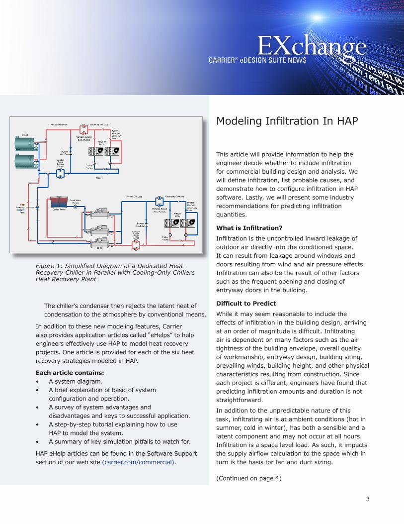
1. Dedicated Heat Recovery Chiller in Parallel with Cooling-Only Chillers - A water-to-water heat pump chiller is placed in parallel with cooling-only chillers. The heat pump chiller operates in heating priority to serve hot water demands. It simultaneously

produces chilled water to serve cooling loads. Cooling-only chillers serve any remaining cooling load. Figure 1, on next page, is a simplified diagram of this particular heat recovery configuration.

2. Air Cooled Chiller with Heat Recovery Condenser - One or more air-cooled chillers are equipped with dual condensers: (1) a refrigerant-to-water condenser to recover heat to serve building heating demands, and (2) a refrigerant-to-air condenser to reject heat to the atmosphere when heat output exceeds heating demand or heating demand does not exist.

3. Heat Exchanger in Condenser Loop - A plate frame heat exchanger is placed between the condenser water loop and hot water loop. Chillers are run at elevated condenser water temperatures in order to allow heat transfer from the condenser loop to the hot water loop via the heat exchanger.

4. Dedicated Heat Recovery Chiller in the Condenser Loop - A water-to-water heat pump chiller is placed between the condenser water loop and the hot water loop. The heat pump chiller operates in heating priority, extracting heat from the condenser loop to heat water in the hot water loop.

5. Chiller with Double Bundle Condenser - One or more water-cooled chillers are equipped with a double-bundle condenser, allowing the chiller to reject heat to the hot water loop when heating demands exist, or to the condenser loop when heating demands do not exist.

6. Chiller with Desuperheater - One or more chillers are equipped with a desuperheater - a heat exchanger at the compressor outlet that recovers high temperature sensible superheat from the discharge refrigerant gas to heat water.


(Continued from page 1)


3

Figure 1: Simplified Diagram of a Dedicated Heat Recovery Chiller in Parallel with Cooling-Only Chillers Heat Recovery Plant

The chiller’s condenser then rejects the latent heat of condensation to the atmosphere by conventional means.

In addition to these new modeling features, Carrier also provides application articles called “eHelps” to help engineers effectively use HAP to model heat recovery projects. One article is provided for each of the six heat recovery strategies modeled in HAP.

Each article contains:• A system diagram.• A brief explanation of basic of system configuration and operation.• A survey of system advantages and disadvantages and keys to successful application.• A step-by-step tutorial explaining how to use HAP to model the system.• A summary of key simulation pitfalls to watch for.

HAP eHelp articles can be found in the Software Support section of our web site (carrier.com/commercial).

Modeling Infiltration In HAP

This article will provide information to help the engineer decide whether to include infiltration for commercial building design and analysis. We will define infiltration, list probable causes, and demonstrate how to configure infiltration in HAP software. Lastly, we will present some industry recommendations for predicting infiltration quantities.

What is Infiltration?

Infiltration is the uncontrolled inward leakage of outdoor air directly into the conditioned space. It can result from leakage around windows and doors resulting from wind and air pressure effects. Infiltration can also be the result of other factors such as the frequent opening and closing of entryway doors in the building.

Difficult to Predict

While it may seem reasonable to include the effects of infiltration in the building design, arriving at an order of magnitude is difficult. Infiltrating air is dependent on many factors such as the air tightness of the building envelope, overall quality of workmanship, entryway design, building siting, prevailing winds, building height, and other physical characteristics resulting from construction. Since each project is different, engineers have found that predicting infiltration amounts and duration is not straightforward.

In addition to the unpredictable nature of this task, infiltrating air is at ambient conditions (hot in summer, cold in winter), has both a sensible and a latent component and may not occur at all hours. Infiltration is a space level load. As such, it impacts the supply airflow calculation to the space which in turn is the basis for fan and duct sizing.

(Continued on page 4)

When Does Infiltration Occur?

Infiltration most often occurs at night when the building is unoccupied and the ventilation (outdoor air) dampers are closed. Since ASHRAE® Standard 62.1 requires ventilation air to be introduced during the building’s occupied cycle, this results in the positive pressurization of the spaces which should offset infiltration.

However, infiltration also occurs when doors remain open as occupants enter and leave. Many existing buildings do not incorporate a vestibule or revolving door to seal off inward leakage. (Did you ever request a table “away from the door” at a restaurant especially in the winter?)

Also, direct exhaust at the space level can offset some of the ventilation air such that less is available to pressurize the space than was originally thought during the occupied cycle. Lastly, stack effect on larger buildings can create infiltration during the day.

Configuring Infiltration in HAP

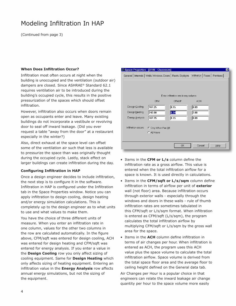
Once a design engineer decides to include infiltration, the next step is to configure it in the software. Infiltration in HAP is configured under the Infiltration tab in the Space Properties window. Notice you can apply infiltration to design cooling, design heating and/or energy simulation calculations. This is completely up to the design engineer as to what units to use and what values to make them.

You have the choice of three different units of measure. When you enter an infiltration rate in one column, values for the other two columns in the row are calculated automatically. In the figure above, CFM/sqft was entered for design cooling, ACH was entered for design heating and CFM/sqft was entered for energy analysis. If you enter a value in the Design Cooling row you only affect sizing of cooling equipment. Same for Design Heating which only affects sizing of heating equipment. Entering an infiltration value in the Energy Analysis row affects annual energy simulations, but not the sizing of the equipment.

• Items in the CFM or L/s column define the infiltration rate as a gross airflow. This value is entered when the total infiltration airflow for a space is known. It is used directly in calculations.

• Items in the CFM/sqft or L/s/sqm column define infiltration in terms of airflow per unit of exterior wall (not floor) area. Because infiltration occurs through exterior walls - especially through the windows and doors in these walls - rule of thumb infiltration rates are sometimes tabulated in this CFM/sqft or L/s/sqm format. When infiltration is entered as CFM/sqft (L/s/sqm), the program calculates the total infiltration airflow by multiplying CFM/sqft or L/s/sqm by the gross wall area for the space.

• Items in the ACH column define infiltration in terms of air changes per hour. When infiltration is entered as ACH, the program uses this ACH value plus the space volume to calculate the total infiltration airflow. Space volume is derived from the total space floor area and the average floor to ceiling height defined on the General data tab.

Air Changes per Hour is a popular choice in that engineers can relate the inward leakage air change quantity per hour to the space volume more easily

Modeling Infiltration In HAP

4

(Continued from page 3)

than units of cfm/sqft of exterior wall or actual cfm.

The Infiltration Occurs item in HAP offers two choices for modeling hourly variation of infiltration airflow:

1. Only When Fan Off. This option will limit infiltration load calculations to those hours during which the fan/thermostat schedule for the system serving the space has been scheduled for the “unoccupied” mode. This option is NOT used to model situations in which the building is positively pressurized during “occupied” hours (which is when the system is running continuously). Therefore, infiltration will only occur during the “unoccupied” hours. (During unoccupied periods, the system actually cycles on and off to maintain the night conditions so this choice really means “during the unoccupied cycle only.”)

2. All Hours. With this option, infiltration loads will be calculated for all hours of the 24 hour day, regardless of whether the system is in “occupied” or “unoccupied” mode. This option is used to model situations in which the building is not pressurized or the negligible when the system is on. As a result, infiltration occurs for all hours of the day.

Industry Findings

Infiltration is a topic that has received a lot of discussion but not a lot of research. The ASHRAE® Fundamentals Handbook, Chapter 16.25 contains interesting information on “Commercial and Institutional Air Leakage.” To summarize their findings, ASHRAE research found that infiltration rates in eight U.S. office buildings ranged from 0.21 to 1.03 CFM/sf (of envelope area) at 0.3” w.g. pressure differential and that typical infiltration rates are 0.10, 0.30 and 0.60 CFM/sf for tight, average and leaky walls.

In addition, ASHRAE Std. 90.1-2013 App G Section G.3.1.5b states that infiltration rates must be calculated as 0.4 CFM/sf of envelope area (@ 0.3” w.g.) and modeled at exactly the same for the Baseline and Proposed building models. Refer to 90.1-2013 App G for more information.

Limiting Infiltration - The New Focus

ANSI®/ASHRAE®/IES® Standard 90.1- 2010 Section 5.4.3 has addressed air leakage through the building envelope. Specific items required are:

1. Continuous Air Barrier - An air barrier shall be installed around the building that resists both positive and negative pressures such as wind, stack effect, and mechanical ventilation

2. Fenestration and Door - Performance requirements are specified

3. Weather Seals - Required where specified such as loading dock doors

4. Vestibule Design - Specific design requirements for both single and multi-story buildings

The goal is to prevent the uncontrolled leakage of air both into and out of conditioned spaces. ASHRAE now seems to focus reduction of air leakage versus providing more data to predict air leakage.

Conclusion

Infiltration results in larger sizes for heating and cooling equipment, ductwork, fans, and associated electrical and mechanical services to serve the equipment. Also, unwanted infiltration can bring thermal discomfort and complaints, increased energy consumption, and even damage due to mold growth.

Predicting infiltration quantity is and will remain a judgment call for the HVAC design engineer. Stringent requirements in ASHRAE 90.1 - 2010 are aimed at reducing the infiltration heat loss and heat gain for a commercial building. Factors like workmanship and testing accuracy of the building envelope will always affect actual results.

If a decision has been made to include infiltration in the building design, HAP will calculate infiltration based on any one of three input parameters that the HVAC engineer feels is applicable.

ANSI® is a registered trademark of the American National Standards Institute

ASHRAE® is a registered trademark of the American Society of Heating, Refrigerating, and Air-Conditioning Engineers, Inc.

IES® is a registered trademark of the Illuminating Engineering Society of North America


5

6

Frequently Asked Questions

Question 1: When defining a Building in HAP, the source electric generating efficiency shown on the Meters tab defaults to 28%. How was this calculated? How do I justify if this is an acceptable percentage? If it is too low, how can it be increased?

Answer: This value is a user input in the Building > Meters tab.

From the HAP Help system:

Source Electric Generating Efficiency

This item defines the average generating efficiency for electric power plants that provide energy to the building. This value is used to calculate “source” energy totals on the two Energy Budget reports. This input is only required if the program will be used to generate the Energy Budget reports and local energy codes require that both “site” and “source” energy totals be provided. If this feature is not needed, set the efficiency to 100%.

Further Details: Energy Budget reports generated by HAP list the “site” and “source” energy use for a building. Site energy is the actual energy consumed by equipment in the building. Source energy is an estimate of the energy required to generate electricity

provided to the building. The difference between site and source energy quantities is due to inefficiencies in generating electricity and transmitting it to the building site. When this is required by energy codes, the codes usually mandate the efficiency value to be used. It typically varies between 25% and 33%. For fuels and non-electric energy sources, site and source energy values are equal since the fuel is consumed at the building site.

NOTE: This is an average value for typical utilities with fossil fuel power plants. If your utility is predominantly hydroelectric or nuclear these numbers would likely change, perhaps dramatically. If you want this efficiency value specifically for your utility you might want to contact them and inquire.

In addition, for most grid-connected power plants distribution line losses of about 6% of transmitted power occur between the plant (source) and the site. Taking the average fossil fuel power plant efficiency as 30%, the overall electric generating efficiency is (0.30) x (1.00 - 0.06) = 0.28 or 28%. That is the basis of the 28% default in HAP.

Question 2: How do I model shading of a window from an adjacent structure in HAP?

Answer: Modeling shading from external structures is a complex analysis and typically requires 3D (x,y,z) spatial coordinates of the adjacent structure surfaces. For example, consider an L-shaped building where one wing of the “L” shades windows on the other wing of the building at certain times of day. The coordinates of the adjacent wall surface relative to a window being shaded need to be known for shading calculations to be performed. HAP currently does not require (x,y,z) spatial coordinates to be specified for wall and window surfaces, but nonetheless there is a way to use the standard external shading geometry inputs in HAP to model a large adjacent shading surface.


7

Basic Concept: Consider the wall surface of the adjacent wing as a vertical shading fin. Typically the shading fin is relatively close to the window (within 12-24 inches or 30-60cm), and the projection of the fin from the wall is similarly relatively small. But HAP allows relative distances and dimensions of the shading fin to be very large. That allows the “fin” to represent a large adjacent wall surface. Steps:

1. For each window, the position of the shading surface relative to the window must be defined. Create one External Shade Geometry item for each window. Viewing the window from outside the building, if the adjacent wall surface is to the left, specify a “Left Fin.” If the adjacent wall surface is to the right, specify a “Right Fin.”

2. Specify “Distance from Edge of Window” to represent the distance from the edge of the window to the wall shading surface. For example in an L-shaped building a particular window might be 50 feet from the wall surface of the adjacent wing. “Distance from Edge of Window” would be specified as 600 inches (50 feet, 15240 mm or 15.24 m). Distances up to 250 ft (76.2 m) are accepted as input.

3. Specify “Projection from Wall Surface” as the length of the wall shading surface. For example in our L-shaped building, the adjacent wing might be 200 feet wide. “Projection from Wall Surface” would be specified as 2400 inches (200 feet, 60960 mm or 60.96 m). Again, distances up to 250 ft (76.2 m) are accepted as input.

4. Finally, specify “Height Above Window” as the distance from the top edge of the window to the top of the adjacent wall shading surface. For example, the window of interest might be on the first floor in a 4-story building, and the distance from the top of the window to the roof level of the adjacent wall might be 40 feet (12.2 m). In this case “Height Above Window” would be specified as 480 inches (40 feet, 12192 mm or 12.192 m). Distances up to 250 ft (76.2 m) are permitted.

Because the relative coordinates of the wall shading surface change for each window being shaded - “Distance from Edge of Window” and “Height Above Window” in particular - steps 1 through 4 above need to be repeated for each individual window on the wall being shaded.

© Carrier Corporation 2015

Carrier University800-644-5544CarrierUniversity@carrier.utc.comwww.carrieruniversity.com

Software Assistance800-253-1794software.systems@carrier.utc.comwww.carrier.com

2015 Training Class Schedule

Location

Phoenix, AZ

Honolulu, HI

Charlotte, NC

Orlando, FL

Pittsburgh, PA

Load

Calculation for

Commercial

Buildings

June 2

Nov 2

Energy

Simulation for

Commercial

Buildings

June 3

Nov 3

Energy Modeling

for LEED® Energy

& Atmosphere

Credit 1

June 4

Nov 4

Sept (dates TBD)

Oct (dates TBD)

Nov (dates TBD)

Advanced

Modeling

Techniques for

HVAC Systems

N/A

Nov 5

Engineering

Economic

Analysis

N/A

Nov 6

Block

Load

N/A

Nov 6

eDesign Suite Software Current Versions (North America)

Functionality

Peak load calculation, system design,

whole building energy modeling,

LEED® analysis.

Rapid building energy modeling

for schematic design.

Peak load calculation, system design.

Lifecycle cost analysis.

Refrigerant line sizing.

Peak load calculation, system design.

Current Version

v4.90

v1.30

v4.16

v3.05

v4.00

v4.90

Program Name

Hourly Analysis

Program (HAP)

Building System Optimizer

Block Load

Engineering Economic Analysis

Refrigerant Piping Design

System Design Load

Additional classes are being added.

carrier® edesign suite news modeling heat recovery

Documents