“Carrier-Gas Enhanced Atmospheric Pressure Desalination (Dewvaporation):

Economic Analysis and Comparison to Reverse Osmosis and Thermal Evaporation”

Noah Abbas and Kehinde Adesoye

Chemical Engineering Undergraduate

University of Oklahoma

4/30/2007

Abstract

With freshwater resources stretched thin, James Beckman of Arizona State

University developed carrier gas-enhanced atmospheric pressure desalination, or simply

“dewvaporation”, which presents a viable option to easing water demands.

Dewvaporation works by evaporating pure water out of seawater with dry air. This now

humid air condenses the pure vapor while donating its heat to seawater aiding in

evaporation for the next cycle. This works to recycle heat and therefore gives it an

advantage over common thermal separation.

A mathematical model composed of differential equations made possible a

description of the process as well as an economic analysis. The results of this analysis

predict a fixed annual cost of about $1867 for a unit producing 1100 gal/day. This

corresponds to a cost of about $2.59/1000gallons. However, this cost considers using

steam to heat the air stream across the top of the tower. Cheaper methods may exist that

utilize solar power or waste heat from an existing plant.

Introduction

Desalination is the process of obtaining water from a solution of salt and water.

This is an important process for the future because of the high demand of pure water in

the world today. The very nature of our existence is dependent on the availability of

water. Making up two-thirds of the earth’s surface, the ocean is the main source water

available. Unfortunately seawater we need is not found fit for human consumption and

has to be acquired one of several technologies. The methods developed today still do not

remove salt from the water perfectly. The water still has some salt in it while the waste

product (brine) has some water in it.

The current methods used for desalination can be classified into two major

categories. These are membrane and thermal methods. Basically, thermal methods are

those in which heat-driven evaporation is the primary source of separation while

membrane methods are those in which a semi-permeable membrane is the main piece of

separation equipment. There are two common examples of these methods which are very

much used in different parts of the world. These are evaporation and reverse osmosis. A

more detailed explanation of these two follows.

World wide uses of these methods are equal at 50%2 each. These methods,

because of their common use, are good standards for comparison with dewvaporation.

Everyday, research and analysis are being carried out to create or evaluate new and

existing technologies for more economical results. Most of these new methods are still

generally stemming from already existing technologies. For example, dewvaporation has

deep roots in the current thermal methods. Generally, most new processes are geared

towards improvement in all areas of desalination.

Existing Technologies

Membrane methods - Reverse osmosis

Membrane methods of desalination rely on the passing of salt water feed through a semi

permeable membrane in order to separate salt from water. The most common membrane

method is Reverse Osmosis. Reverse osmosis is a method of desalination where the feed

solution is forced through a semi-permeable membrane resulting in the passage of high

water content solution and leaving behind a highly concentrated salt solution. Physically,

solutions flow from a high to low concentration region (osmosis), but the application of

pressure yields the opposite and water flows from the solution through the membrane

(reverse osmosis). The applied pressure has to be greater than the normal osmotic

pressure of the salt water. Osmotic pressure is as the pressure a solution exerts on a

membrane in an enclosed space due to the difference in solute concentration between

both sides of the membrane. As mentioned earlier, this process does not yield totally pure

water, the water and salts travel at different rates through the membrane. A schematic of

this process is shown below.

Fig. 1: A typical reverse osmosis plant

Pump

Membrane

Module

Brine

Pretreatment Post

Treatment

Saline Feed

Pure

Water

Usually, the process consists of four major parts. The first is the pretreatment

stage. This is necessary for most membrane methods because of the settling of

microorganisms and different particles in the feed water solution on the membrane

causing fouling. Various methods of pretreatment include addition of chemicals such as

chlorine to kill these microorganisms or ultra-filtration to separate them out. Pretreatment

also involves the addition of anti-scalants to prevent scaling on the membrane surface.

Scaling is the forming of salt precipitates such as calcium carbonate on the surface of the

membrane due to the concentration of salt ions at the membrane surface resulting in

saturation and then precipitation. This reduces the ability of the membrane to separate the

salt and water. Examples of anti-scalants include sulfuric acid.

The second is the pumping stage where the saline feed pressure is raised to the

calculated optimum for that plants operation. It must be larger than the osmotic pressure

of the saline feed. The third is the actual separation process in the membrane module.

During separation, not only one membrane is present, there are several layers of

membranes and several units of these membranes giving them the term modules. A

stream of pure water and another of brine leave this section. The last stage is the post

treatment stage. Post treatment in reverse osmosis desalination involves the use of salts

such as calcium and sodium to alleviate the effect of the acid added in the pretreatment

stage.

Calculated costs associated with reverse osmosis include the following:

Table 1: Reverse Osmosis Costs5,6

Desalination

method

Expected

recovery (%)

Operating cost

($/1000gal of product)

Capital cost

($/gal-day)

Energy requirements

(KWh/1000gal of product)

Reverse osmosis 50 2.50 – 4.00 4.00 - 10.00 26

The major source of expenditure is the membrane used. This is a complex web of

polymers designed to allow the passage of water while preventing the passage of salts to

an extent. Various designs have being suggested to increase the selectivity of these

membranes but these designs increase in price as they get better. Also because of fouling

and scaling, membrane designs are being evaluated for their performance levels also

increasing the cost of a membrane. A membrane lifetime is a maximum of two years and

usually need changing after that.

Thermal methods – Multi Stage Flash Desalination

These are processes involving the heating of salt water to evaporate the pure water and

condense it. This basic process has being in existence for centuries and is the first method

of desalination to be used in earlier forms such as boiling. Over the years, modifications

of this desalination process have being in effect and currently the most used type is the

Multi-Stage Flash Distillation (MSF). Currently, 80%7 of the world’s thermal

desalination products are from MSF desalination.

In this process, the salt water is first heated at high pressure and then transferred

into a chamber at a reduced pressure. Due to the drop in pressure at the beginning of each

chamber, the boiling temperature of water reduces causing it to evaporate. This process

of quick evaporation is usually referred to as ‘flashing’. Condensation of the vapor takes

place on the tubes of a heat exchanger that passes through the chamber. The heat

exchanger uses the feed water to cool the vapor before the feed enters the chambers. The

heat of vaporization during condensation is then transferred back to the feed stream and

the cycle continues. The flash chambers usually are between 15 and 252. The heat

released through vaporization makes this process able to use low heat sources to heat up

the feed at the start of the process. A schematic of the process can be seen below.

Fig 2: Schematic of Multi Stage Flash Desalination

Advantages of this process include the low cost of energy with availability of

waste heat and the insignificance of the quality of the saline feed reducing pretreatment

costs. Problems associated with the MSF method are high operating costs with no waste

heat available, corrosion and erosion. Corrosion and erosion are caused by the fact that

water is being passed through metal pipes, and also because of the speed at which the

water moves. The use of metals in this process is inevitable as high conductivity of heat

is especially needed for high yield. The use of stainless steel is very common to prevent

corrosion but this is very cost intensive. MSF plants are usually found in the Middle East

because of the large availability of cheap energy.

The major money guzzler for this process is the heat required to heat the salt

Waste

Brine

Condensate

Trays

Heat Vapor

Saline

Feed

Pure

Water

Pump

Heat

Exchanger

water. This is very much the main drive of the process and directly impacts the

production capacity. The following are some statistics about the MSF process.

1. Expected recovery – 20-30%

2. Associated costs – $12-$14/1000gal of product4

3. Energy requirements – 56KWh/1000gal of product5

A general description of the proportions in which these methods are being used in the

world compared to other membrane methods or thermal methods can be seen in the

following chart.

Distribution of desalination process in the world

Fig.3: Distribution of desalination processes used in the world

For these two major processes, the lifespan of a typical plant should be well

looked at. Even though thermal processes may seem to be more expensive than

membrane processes, their lifetimes are more than twice the lifetime of a membrane.

RO

(90%3 membranes)

Other

(10% membrane)

MSF

(84%6 thermal)

Other

(16% thermal)

Waste Disposal Techniques

Waste disposal methods in desalination are very particular to the system being

used and the surroundings in which they are used. In this paper, only the system used will

be used to evaluate different disposal methods as no particular plant is in consideration.

Waste from desalination plants can generally be divided into three parts. These are the

pre-treatment, actual process and post-treatment waste. The pretreatment methods

discussed above for the reverse osmosis plant is very similar to those of the MSF method

except for the concern of microorganisms and suspended particles fouling any part of the

system. The ultra filtration of these require correct disposal. Most pretreatment wastes are

solids although anti-scalant and chemical addition can constitute liquid waste.

The actual process waste varies depending on whether it is a thermal or

membrane process. For thermal processes, the wastes include concentrated brine and

dried salts. Some methods of disposal are returning the brine to its source, brine

evaporation and deep-well injection. Some gases may appear, examples of which are

carbon dioxide, oxygen and nitrogen. These require no special disposal method.

Membrane processes on the other hand produce less concentrated brine waste but have

membrane modules to dispose off as solids waste. The brine waste can be disposed in a

similar manner as the thermal methods. The membrane modules have no health hazards

or risk therefore they are placed in sand fills. Post treatment wastes are similar to those

obtained from pre treatment wastes and cane be disposed of in the same way.

Dewvaporation

This is a process invented recently by James Beckmann, an associate professor of

chemical engineering at Arizona State University. It uses novel ideas to implement salt

water desalination in the direction of thermal methods. The whole process is carried out

in atmospheric pressure and it uses air as a carrier gas for the water vapor. The heat

source can come from waste heat from an existing plant possibly bringing the heat costs

to zero. This process promises lower costs for saltwater desalination through this ability

to cut down on energy cost. The process flow diagram can be seeing below in Fig. 4 and

a description given.

Fig. 4: The flow diagram of a typical dewvaporation process

P

u

r

e

w

a

t

e

r

S

a

l

i

n

e

f

e

e

d

Inlet

Air

Blower

Added heat

(Qboiler)

Heat

Condensing water

Saline feed

Air

Evaporating water

Outlet

Air Ambient

Air

Process description

In this process, ambient air of known temperature and humidity is pumped at a

constant rate into the bottom of the evaporation chamber of the dewvaporation tower. As

air flows up, simultaneously, saline feed is flowing down from the top of the tower on the

same side along the heat transfer wall. Heat transfer occurs between the wall and the

saline feed and water evaporates from the solution into the ambient air serving as a

carrier gas. Concentrated salt water exits the tower from the bottom of the evaporation

side. The air, which has now increased in temperature and humidity flows from the top of

the tower. An external heat source is used to raise the temperature of the air before the air

flows down the dewformation side of the tower. Using steam as a heat source increases

the humidity of the air that goes into the dewvaporation side allowing more water to

condense. The increased temperature of the air from heating allows for this side to be

slightly hotter than the evaporation side initiating condensation and transfer of

condensate heat to the evaporation side through the wall. Both Pure water and air at

reduced temperature flow from the dewformation side of the tower. The air can be

recycled into the incoming air stream and pumped back into the system.

Economic analysis

The main objective in developing new technologies for desalination is to reduce cost. For

most desalination process, the two most important cost components calculated are the

operating and capital costs. The operating cost is the cost of running the process daily. It

is usually expressed as cost per unit energy or cost per unit of production. The capital

cost is that which comes from the equipment used in production. The capital cost

estimation usually comes from the calculation of some property of the equipment such as

area or capacity while the operating cost comes from a parameter that directly impacts the

production such as heat or pressure. In this case the heat added to the system is used. The

addition of these costs gives the total annual cost of the process. The first step in these

cost estimations was the derivation of mass and heat balances.

Tower Mathematical Model

The first step in designing the tower is generating the necessary operating

parameters such as temperature and flow rate settings. In the absence of a pilot plant, a

mathematical model gives the best estimates of these parameters and also makes some

optimization possible. For the dewformation tower, differential equations are adequate to

describe the heat and mass transfer.

Building a model of differential equations for the tower requires defining a

differential portion of the tower. The following diagram displays the boundaries of the

region:

Fig. 5: Differential Set Up

T1 = T5 +∆T

Air

Ve

1 2 3 5 4

dz

T5

z

z+dz T2 + dT

T2 q

T5

T5 + dT

dWe Air

Vd

G

FD FB

dWd

G

This tower is divided regions one through five. The first region is the humid air

containing the pure water vapor. As it dumps off heat to region two, its water vapor also

condenses into this region (dWd). Region two is therefore the pure water product (FD).

The heat of condensation of the water on the wall then moves over to the fourth region.

The fourth region is the seawater feed (FB) running along the wall on the evaporation

side. It receives the heat and is exposed to the dry air of region five. This forces the

evaporation of water (dWe) into region five.

V refers to the gas loading in units of moles of water vapor/ moles of air, while Vs

refers to the saturation gas loading. G is the flow rate of air minus the water vapor it

contains and is constant throughout the apparatus.

Integrating the mass and heat balances on this diagram describe the system from

top to bottom. The mass and heat balances started with the following analysis:

Region Mass balance Heat balance

1 ddzzz dWGVGV += + dzTThLdWhdTTGVhdTTGhTGVhTGh dvapVava )()()()()( 211111 −+∆++++=+

2 dzzdz FDdWFD +=+ qdTThFDdzTThLdWhThFD wdzzdvwz +−=−+∆+ + )()()( 22212

3 0 dzTTULq )( 42 −=

4 edzzz dWFBFB += + )()()( 5444 TThLdWhdTThFBqThFB evwdzzwz −+∆+−=+ +

5 edzzz dWGVGV += + )()()()()( 55545555 TGVhTGhdzTThLdWhdTTGVhdTTGh vaevapVa +=−+∆++++

Table 2. Mass and Heat Balances

For example, the mass balance on the first region has terms accounting for the water

vapor inputs and outputs to the region along with the small amount of water dumped off

into the pure water product flow. The same quantity of air (G) goes into and out of the

region such that the term cancels. The heat balance has terms accounting for the enthalpy

of air (Gha(T1)) and water vapor (GVhv(T1)) that enter the region. Exiting the region is

the new enthalpy of the air and water vapor as well as the heat leaving with the

condensed vapor (∆hvapdWd) and also the heat given to region two due to the temperature

difference (hL(T1-T2)dz).

The next step is to convert these equations into differentials that can be solved in

a step wise fashion. The derivations ran as follows:

Region 1

Mass balance

dDZZ dWGVGV += +

dzzzd GVGVdW +−=

11

dTdT

dVGdW

s

d =

Heat balance dzTThLdWhdTTGVhdTTGhTGVhTGh dvapVava )()()()()( 211111 −+∆+−+−=+

dzTThLdWhdTTGVhTGVhdTTGhTGh dvapVvaa )()()()()( 211111 −+∆=−−+−−

dzTThLdWhdTCpGVdTGCp dvapvs

air )( 2111 −+∆=+

Substituting the mass balance,

dzTThLdTdT

dVGhdTCpGVdTGCp

s

vapvs

air )( 2111

11 −+∆=+

1

211

)(

dT

dVGhCpGVGCp

dzTThLdT

s

vapvs

air ∆−+

−=

Note: sVV < then shh = , 01

=dT

dV s

and 3TT =

Region 2

Mass balance

dzzdz FDdWFD +=+

Note: mass balance = 0 until sVV >

Heat balance

qdTThFDdzTThLdWhThFD wdzzdvwz +−=−+∆+ + )()()( 22212

Rearranging and substituting with the mass balance qdzTThLdWhdTThdWFDThFD dvwdzwz =−+∆+−+− )()()()( 21222

dzTTULqdzTThLdWhdTThdWdTThFDThFD dvwdwzwz )()()()()( 422122222 −==−+∆+−−−−dzTTULdzTThLhdTThdWdTCpFD vwdwz )()())(( 4221222 −=−+∆+−−

Region 4

Mass balance

edzzz dWFBFB += +

Heat balance

outevwdzzinwz qdWhdTThFBqThFB +∆+−=+ + )()( 33

Substituting mass balance

outevwdzzinwz qdWhdTThFBqThFB +∆+−=+ + )()( 33

outevinwezwz qdWhqdTThdWFBThFB +∆=++−− )()()( 33

outinevwewz qqdWhdTThdWdTCpFB =+∆−++ )( 33

dzTTLhdzTTLhdWhdTThdWdTCpFB evwewz )()()( 5445422433 −=−+∆−++

wz

weev

CpFB

dTThdWdWhdzTTLhdzTTLhdT

)()()( 4422454454

+−∆+−−−=

Region 5

Mass balance

edzzz dWGVGV += +

55

dTdT

dVGdW

s

e =

Heat balance )()()()()( 55545555 TGVhTGhdzTThLdWhdTTGVhdTTGh vaevapVa +=−+∆+−+−

dzTThLdWhdTTGVhTGVhdTTGhTGh evapVvaa )()()()()( 54555555 −−=∆+−−+−−

dzTThLdWhdTCpGVdTGCp evapairs

air )( 5455 −−=∆++

dzCpFD

TThL

CpFD

TTUL

CpFD

hdTThdWdT

wzwzwz

vapwd

−−

−+

∆+−=

)()())((214222

2

dzTThLdTdT

dVGhdTCpGVdTGCp

s

vapairs

air )( 5455

55 −−=∆++

5

545

)(

dT

dVGhCpGVGCp

dzTThLdT

s

vapvs

air ∆++

−−=

The results are summarized in the following table:

Table 3. Results of Mass and Heat Balances

Region Mass Balance Heat Balance

1 1

1

dTdT

dVGdW

s

d =

1

211

)(

dT

dVGhCpGVGCp

dzTThLdT

s

vapvs

air ∆−+

−=

2 dzzdz FDdWFD +=+

4 edzzz dWFBFB += +

wz

weev

CpFB

dTThdWdWhdzTTLhdzTTLhdT

)()()( 4422454454

+−∆+−−−=

5 5

5

dTdT

dVGdW

s

e =

5

545

)(

dT

dVGhCpGVGCp

dzTThLdT

s

vapvs

air ∆++

−−=

In certain cases these equations make take different forms. For example, the

result of the heat balance on region one only takes the form shown in Table 3 when Vd

exceeds Vsd. This indicates that the air is currently holding more water than is possible

given the saturation gas loading. It must therefore dump off water to region two,

resulting in bulk heat transfer. When it is lower, the last term in the denominator is zero

because no water moved across the boundary of regions one and two in that differential

step. This may be the case when hot humid air first enters the top of the tower on the

dzCpFD

TThL

CpFD

TTUL

CpFD

hdTThdWdT

wzwzwz

vapwd

−−

−+

∆+−=

)()())((214222

2

dewformation side and has yet to experience significant cooling. However, when the

heating is done via adding steam, the air stream remains saturated even though it is at a

higher temperature. This is the case in the model presented here. The same situation

arises in region five regarding the last term in its denominator and Ve’s relationship to

Vse.

The heat and mass balances on region three are trivial and not displayed. The

only affect region three has on the heat transfer is to alter the heat transfer coefficient

between regions one and two. When Vsd exceeds Vd, no water product has formed and

therefore region two does not exist. The resulting heat transfer coefficient is the result of

air’s forced convection with metal rather than air’s forced convection on water.

Solving the Model

Microsoft Excel put the model to the test. The spreadsheet takes the equations

and integrates them from the top of the tower to the bottom. Starting at the top of the

tower, the user has several variables that he may manipulate as settings for column

operation. These include Q, ∆z, Z, G, FB, L, T5 top, and T4 top.

Q is the heat added to the air stream as it crosses over the top of the column from

the evaporation side to the dewformation side. Because the heat goes in as steam, the air

is still saturated as it enters the other side even though its temperature is slightly higher.

The amount of water it holds also increases because of the water added as steam. ∆z is

the incremental height of the column and therefore refers to the step size of each

calculation as the integration moves down the tower. Its summation gives the height of

the tower. G is the air flow up the evaporation side and down the dewformation side and

is constant throughout the tower. FB is the feed flow rate of the seawater/brine, L is the

width of the tower, T5 if the temperature of the air as it exits the top of the evaporation

side, and T4 is the temperature of the feed. T4 is not very flexible since the user is

restricted to using ocean temperatures near his plant.

The results of this integration include the heat required as well as the necessary

heat transfer area of the column. These are the two main cost parameters in designing the

column. To start the integration the spreadsheet had the following headings:

Table 4. Spreadsheet Headings and Layout*

*Note: James Beckman’s numbers for the saturation humidity did not agree with those found in Perry’s

Chemical Engineers Handbook. The results reported here are using saturation calculations from Perry’s.

Otherwise the spreadsheet gives no significant product flow rate.

The spreadsheet keeps track of all relevant parameters and variables needed in calculating

them as it integrates down the column. It has a column for the temperature changes, mass

exchanges, and humidity based on temperature down the column.

Results

The first result to consider from the spreadsheet is the temperature profile. When

the temperatures follow expected trends and match existing data, the model gains

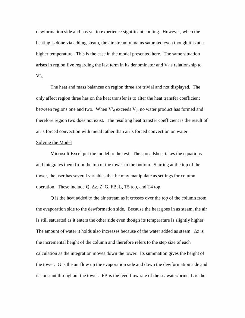
credibility. Figure 6 displays the temperature profile down the column:

Temperature Down the Tower

0.00

10.00

20.00

30.00

40.00

50.00

60.00

70.00

80.00

0 100 200 300 400 500 600 700 800

Distance from Tower Top (cm)

Tem

per

atu

re (

deg

. C

)

T Air Dewformation Side

T Pure Water Product

T Seawater/Brine

T Air Evaporation Side

Fig. 6: Temperature profile down the tower.

This graph concisely displays the trends in temperature. The air on the

dewformation side decreases in temperature as it gives off heat to the rest of the column

as expected. The pure water product also looses more heat than it gains, so its

temperature also declines. The brine warms slightly as it evaporates. Most importantly,

the air on the evaporation side sees its temperature fall to roughly that of ambient air.

This is critical because the entry temperature of the air on the evaporation side is not

adjustable by the user. Lowering this temperature to ambient air temperature is what

establishes “the end” of the column. This figure suggests that the column must be about

7.2m high, which is number that may change as operating variables change.

Once the temperature profile lends validity to the model and the current settings,

the calculations present other relevant production numbers. These include the flow rate

of product and brine that must be disposed as well as the air flow throughout the column.

Air flow seemed to have the most dramatic influence on the production flow rate, column

height, and heat required to run the tower. The results of varying air flow are displayed

in the following table and figures:

Table 5: Tower Results

Design G mol/h

Qboiler J/hour FD gal/day FB gal/day FAC $

Cost $/1000gallons

1 1000 290700 187.85 954.77 $1,557.14 $2.59 2 2000 581400 272.06 870.56 $1,665.91 $1.92 3 3000 872100 562.05 580.56 $1,725.26 $0.96 4 4000 1162800 749.33 393.29 $1,773.35 $0.74 5 5000 1453500 936.60 206.01 $1,830.24 $0.61 6 6000 1744200 1123.76 18.85 $1,867.10 $0.52

Product Flow vs. Air Flow

0

200

400

600

800

1000

1200

0 1000 2000 3000 4000 5000 6000 7000

Air Flow Mol/hr

Pro

du

ct F

low

gal

/day

Fig. 7: Product Flow vs. Air Flow

FAC vs. Air Flow

1000.00

1100.00

1200.00

1300.00

1400.00

1500.00

1600.00

1700.00

1800.00

1900.00

2000.00

0 1000 2000 3000 4000 5000 6000 7000

Air Flow mol/hr

FA

C $

Fig. 8: FAC vs. Air Flow

An interesting observation is that the model predicts very little change in flow rate

(Less than a half a gallon/day for each 5C) when altering the temperature increase of the

air across the top of the tower. This is probably because under additional heating the

humid air on the dewformation side must experience more cooling to drop off the same

amount of water. However, the air flow results in large changes because exposure to

more air forces more drying.

Upping the air flow also increases flow rate of product. Because the flow rate of

the product is higher, the brine flow rate is lower thus leading to savings on brine

disposal. Therefore, the benefits of increasing the flow rate, that is, a higher product flow

and less brine disposal, far outpace the downside, which includes higher energy cost and

larger process equipment.

Another important factor in design consideration is the concentration of the brine

at the tower exit. If this concentration should fall below the solubility of salt in water

(374 g/L), crystals will form on the inside of the tower. This is obviously undesirable

because it can cause blockage and therefore the flow may back up. The following table

considers this important aspect of each design.

Table 6. Design Feasiblity Design Seawater Flow L/hr Total Salt g/hr Brine Flow L/hr Brine Concentration g/L

1 180 5406 151 35.9 2 180 5406 137 39.4 3 180 5406 92 59.0 4 180 5406 62 87.2 5 180 5406 32 166.4 6 180 5406 3 1818.2

The findings in Table 6 unfortunately indicate that design six is not a possibility because

the concentration exceeds the solubility limit of salt in water.

The model predicts a price per 1000 gallons of about $2.59 when considering heat

requirements and brine disposal. This falls within the range of $3.70 to $1.70 predicted

by James Beckman’s pilot plants10 and is competitive with existing methods such as

reverse osmosis and evaporation.

Discussion and Conclusion

Dewvaporation is one of several solutions to growing water demands. Further

research into the implementation of solar energy to make the process even cheaper can

make the process more appealing to communities looking to add to their current water

production. According to this mathematical model, air flow is the most important

production parameter when considering a dewvaporation plant.

Definitions of Notations and Variables

dWd Differential Amount of Water Added to FD

dWe Differential Amount of Water Evaporated

FB Seawater Flow

FD Pure Water

G Air Flow

T Temperature

V Gas Loading (moles water vapor/ moles of air)

Vs Gas Loading at saturation humidity

Q Heat

Z Column Height

References

1. Miller, James E. “Review of Water Resources and Desalination Technology”.

March 2003. Albuquerque, NM.

http://www.sandia.gov/water/docs/MillerSAND2003_0800.pdf

2. Krishna, Hari J. “Introduction to Desalination Technology”.

http://www.twdb.state.tx.us/Desalination/The%20Future%20of%20Desalination

%20in%20Texas%20-%20Volume%202/documents/C1.pdf

3. Beckman, James. “Carrier Gas-Enhanced Atmospheric Desalination: Final

Report”. Arizona State University. October 2002.

4. Chaudhry, Shauhid. “Unit Cost of Desalination”.

http://www.owue.water.ca.gov/recycle/desal/Docs/UnitCostofDesalination.doc

5. R. W. Baker et al. Membrane Separation Systems. 1991, Noyes Data

Corporation.

http://www.knovel.com/knovel2/Show_Text.jsp?SetID=5950749&SpaceID=0&V

erticalID=0&BookID=312&NodeID=1885127923&SearchType=0&SearchMode

=true&HTML=false&TextID=2&Random=541172436

6. US Army Corps of Engineers. “Waste Disposal”.

http://www.usace.army.mil/publications/armytm/tm5-813-8/c-10.pdf (waste

disposal)

7. http://www.hwsdesalination.com/multi%20stage%20flash%20desalination.html

8. Frenkel, Val. “Desalination Methods, Technology, and Economics”. Kennedy and

Jenks Consultants

http://www.idswater.com/Common/Paper/Paper_90/Desalination%20Methods,%

20Technology,%20and%20Economics1.htm (diagrams)

9. Beckman, James and Bassem .M. Hamieh. “Seawater Desalination Using

Dewvaporation Technique: Experimental and Enhancement Work with

Economic Analysis.” Arizona State University. September 2003.

http://www.desline.com/articoli/6604.pdf (Dewvaporation)

10. Desalination , Multistage Flash.”

http://www.uwec.edu/piercech/desalination/MSF.htm

11. Peters, Max S. and Klaus Timmerhaus. Plant Design and Economics for

Chemical Engineers. McGraw-Hill 2003.

12. Winnick, Jack. Chemical Engineering Thermodynamics. John Wiley & Sons.

1997.

13. Welty, James R. et al. Fundamentals of Momentum, Heat, and Mass Transfer.

4th edition. John Wiley & Sons 2001.

14. Perry, R. H. Editor. Perry’s Chemical Engineers Handbook. 7th Edition.

McGraw-Hill 1997.

15. EPA. “Drinking Water Advisory: Consumer Acceptability Advice and Health

Effects Analysis on Sodium”. February 2003.

16. Patnaik, Pradyot. Handbook of Inorganic Chemicals. McGraw-Hill. November