carroll, s.p. and owen, j.s. and hussein, m.f.m. (2014)...
TRANSCRIPT

Carroll, S.P. and Owen, J.S. and Hussein, M.F.M. (2014) Experimental identification of the lateral human–structure interaction mechanism and assessment of the inverted-pendulum biomechanical model. Journal of Sound and Vibration, 333 (22). pp. 5865-5884. ISSN 0022-460X
Access from the University of Nottingham repository: http://eprints.nottingham.ac.uk/35568/1/Manuscript_SPCarroll_JSV.pdf
Copyright and reuse:
The Nottingham ePrints service makes this work by researchers of the University of Nottingham available open access under the following conditions.
This article is made available under the Creative Commons Attribution Non-commercial No Derivatives licence and may be reused according to the conditions of the licence. For more details see: http://creativecommons.org/licenses/by-nc-nd/2.5/
A note on versions:
The version presented here may differ from the published version or from the version of record. If you wish to cite this item you are advised to consult the publisher’s version. Please see the repository url above for details on accessing the published version and note that access may require a subscription.
For more information, please contact [email protected]

Experimental identification of the lateral human-structure interactionmechanism and assessment of the inverted-pendulum biomechanical model.
S.P.Carrolla,∗, J.S.Owena, M.F.M.Husseinb
aCentre for Structural Engineering and Construction (CSEC),University of Nottingham, University Park, Nottingham, NG7 2RD, United Kingdom
bInstitute of Sound and Vibration Research,University of Southampton, Highfield Campus, Southampton, SO17 1BJ, United Kingdom
Abstract
Within the context of crowd-induced lateral bridge vibration, human-structure interaction (HSI) is a widelystudied phenomenon. Central to this study is the self-excited component of the ground reaction force (GRF).This force harmonic, induced by a walking pedestrian, resonates with lateral deck motion, irrespective ofthe pedestrian’s pacing frequency. Its presence can lead to positive feedback between pedestrian GRFs andstructural motion. Characterisation of the self-excited force as equivalent structural mass and damping hasgreatly improved the understanding HSI and its role in developing lateral dynamic instability. However,despite this evolving understanding, a key question has remained unanswered; what are the features of apedestrian’s balance response to base motion that give rise to the self-excited force? The majority of theliterature has focused on the effects of HSI with the underlying mechanism receiving comparatively littleattention. This paper presents data from experimental testing in which 10 subjects walked individually on alaterally oscillating treadmill. Lateral deck motion as well as the GRFs imposed by the subject were recorded.Three-dimensional motion capture equipment was used to track the position of visual markers mounted onthe subject. Thus whole body response to base motion was captured in addition to the GRFs generated.The data presented herein supports the authors’ previous findings that the self-excited force is a frequencysideband harmonic resulting from amplitude modulation of the lateral GRF. The gait behaviour responsiblefor this amplitude modulation is a periodic modulation of stride width in response to a sinusoidally varyinginertia force induced by deck motion. In a separate analysis the validity of the passive inverted pendulummodel, stabilised by active control of support placement was confirmed. This was established throughcomparison of simulated and observed frontal plane CoM motion. Despite the relative simplicity of thisbiomechanical model, remarkable agreement was observed.
Keywords: human-induced vibration, biomechanics, motion capture, footbridge, amplitude modulation,lateral dynamic instability, inverted pendulum
1. Introduction
Field observations of bridges exhibiting large amplitude lateral oscillations under the influence of pedes-trian traffic have grown in number [1, 2, 3, 4, 5] since the publication of Dallard et al’s discussion of London’sMillennium Bridge [6]. A central theme linking these loading events is that the response amplitudes ob-served are uncharacteristically large considering the number of pedestrians present on the structure. Thusthe logical conclusion is that some form of positive feedback is occurring between the walking crowd andthe oscillating structure. The unknown nature of this interaction continues to motivate research efforts.
∗Corresponding author. Tel: +44 (0)115 846 8933Email address: [email protected] (S.P.Carroll)
Preprint submitted to Elsevier April 14, 2014

The initial assumption of an interaction mechanism based on step synchronisation between pedestriansand an oscillating bridge deck is now thought to be preceded by a more subtle interaction [4, 5]. This human-structure interaction (HSI) (as opposed to human-structure synchronisation) results in a force harmonicwithin the ground reaction force (GRF) spectrum, that resonate with bridge deck motion [7]. These forceharmonics are referred to as self-excited forces due to their dependence on and resonance with, deck motion.
Based on an extensive experimental campaign, Ingolfsson et al. [8] have further characterised the self-excited force as a mass and damping influence on the oscillating structure. Despite these advances, afundamental question has remained unanswered; what is the lateral HSI mechanism? Put another way,what is it about a pedestrian’s balance response to base motion that gives rise to the self-excited force? TheGRF (of which the self-excited force is a component) is a direct result of body mass accelerations, which arethemselves determined by the pedestrian’s response to deck motion. As such, to further understand HSI,one must first consider pedestrian stability and balance behaviour while walking in the presence of lateraldeck motion.
An experimental campaign was therefore designed in which test subjects walked on a laterally oscillatingtreadmill. A range of tests were carried out, with varying oscillation frequencies and amplitudes imposedon the deck. GRFs were directly measured using deck-mounted load cells. In addition, each subject wasinstrumented with 31 active visual markers in order to record 3-dimensional whole body motion. In broadterms, the objective of this campaign is to not only capture the GRFs generated while walking on anoscillating deck, but also to identify the associated balance behaviour responsible for their generation.
Preliminary results relating to two participants in this campaign have been previously reported by theauthors [9]. That preliminary data set identifies foot placement position as being central to the developmentof the self-excited force. Amplitude modulation (AM) was identified as the mechanism through whichsideband force harmonics are generated in the GRF spectrum. One of the sidebands was identified as theself-exited force harmonic. The data and discussion presented herein further support these preliminaryfindings.
Understanding the HSI mechanism is itself an important milestone, however developing robust interactionmodels based on this understanding offers the ability to predict future bridge response. Attempts to modellateral HSI have been greatly advanced by Macdonald’s investigation of the inverted pendulum biomechanicalmodel [10]. This single degree of freedom model, actively stabilised on a step-by-step basis [11, 12, 13],through control of pendulum support position, allows HSI to be directly simulated. Macdonald’s modellingapproach has been adopted by others, including the authors of this work, for the simulation of multi-pedestrian HSI [14, 15, 16]. However, there remains a question regarding the validity of the centre of mass(CoM) motion simulated by the inverted pendulum model on an oscillating structure. The source of thisuncertainty will be elaborated on below.
The motion capture data obtained in this campaign allows the trajectory of the pedestrian’s CoM tobe estimated and tracked. This provides an excellent opportunity to compare observed CoM motion withthat predicted by the inverted pendulum model. Thus the uncertainty regarding inverted pendulum modelvalidity will also be addressed in this paper.
In section 2 details of the experimental test campaign are provided including a brief description of themotion capture equipment, marker placement and the oscillating treadmill test rig. Data acquisition andprocessing is discussed in section 3. Section 4 contains an analysis of experimentally observed gait behaviourand further supports the authors previous analysis [9], linking gait behaviour to the self-excited force. Thisis followed by an assessment of the validity of the inverted pendulum biomechanical model for use on anoscillating deck. The assessment is facilitated by the direct comparison of experimentally observed andsimulated CoM motion. Finally, section 6 summarised the main conclusions.
2. Experimental investigation
The experimental campaign required test subjects to walk (individually) on a laterally oscillating tread-mill. During each test, the lateral component of the GRF was measured using 4 deck mounted Zemic bendingbeam load cells (490 N capacity each). Lateral deck displacement and acceleration were also recorded via
2

a linear variable differential transformer (LVDT) and Schaevitz linear servo accelerometer. The position of31 visual markers, mounted on the test subject was simultaneously recorded using a Coda mpx30 general-purpose 3D motion tracking system.
All testing was carried out at the University of Nottingham’s Human Performance Laboratory betweenMarch and May of 2012. The test protocol received ethical approval from the Faculty (of Engineering) Re-search Ethics Committee within the University of Nottingham. Ten subjects took part in the test campaign.The age, height and weight of all participants is shown in table 1. The majority of anthropometric datain the literature has been obtained from male subjects. To ensure congruency and in order to utilise thisdata as effectively as possible, only male subjects were recruited for this campaign. This is justifiable whenone considers that there is no reason to suspect that male subjects will behave (statistically) significantlydifferently to female subjects. It is therefore assumed, until proven otherwise, that the behaviours observedand conclusions drawn are equally applicable to both sexes.
Table 1: Test subject data.
Subject Height (m) Mass (kg) Age (Years)1 1.73 82.05 282 1.82 96.20 303 1.74 63.05 274 1.84 98.95 285 1.68 85.45 346 1.88 90.95 217 1.82 87.20 268 1.61 75.00 319 1.80 74.05 2810 1.76 82.70 34Mean 1.77 83.11 28.7
The test protocol for an individual subject was as follows;
• The subject was familiarised with the oscillating treadmill and all safety procedures.
• The subject was instrumented with gait analysis wands and visual markers.
• The subject had a further unrecorded period of familiarisation walking on the treadmill without lateralmotion, lasting approximately 10 minutes. During this time a comfortable walking speed was selectedby the subject.
• The subject was then recorded walking without lateral motion imposed on the deck. This data servedas a baseline for the subject’s walking behaviour.
• After baseline tests were completed, the subject was recorded walking while lateral oscillations wereimposed on the deck, referred to hereafter as dynamic tests. For all dynamic tests, the subject walkedat a speed that was self selected for each test. This speed was maintained throughout each 20 secondtest.
• Rest breaks were imposed every 2-3 minutes during the course of the test session.
Five oscillation amplitudes were tested, 5 mm, 10 mm, 20 mm, 35 mm and 50 mm. Within eachamplitude, 9 oscillation frequencies were tested ranging from 0.3 Hz to 1.1 Hz in 0.1 Hz increments, resultingin a 45 point test matrix.
3

2.1. Oscillating treadmill test rig
The design of the oscillating treadmill test rig, Fig. 1 (a), hereafter referred to as ‘the rig’, and validationof GRF data obtained from the rig, have been reported in [9]. Therefore a concise functional descriptionof the apparatus is provided herein. The rig consists of three frames, Fig. 1 (d). The base frame is thelowermost frame and remains stationary. The chassis frame rests on 4 carriages that travel along linearguide rails fixed to the base frame. The chassis frame is driven laterally in a sinusoidal reciprocating motionby a drive arm connected to the motor, see Fig. 1 (b). The uppermost treadmill frame is suspended fromthe chassis frame by 4 hangers, Fig. 1 (c). The self-weight of the treadmill frame and any vertical imposedloads are resisted by the hangers. The treadmill frame is restrained laterally by 4 bending beam load cells,the means through which the lateral GRF is recorded. The treadmill belt is driven by a second motor (notshown) mounted on the chassis frame. The deck walking area measures 1 m wide × 1.5 m long. A horizontalbar/handle was placed across the front of the treadmill to provide extra stability should a test subject feelparticularly unstable. Subjects were instructed not to touch the bar unless absolutely necessary, after whichthe test data was discounted.
2.2. Motion capture system
A Coda 3D motion tracking system was used [17], consisting of 2 measurement units, each containing 3pre-aligned cameras, wall mounted on either side of the test rig. The cameras track the position of activemarkers (infra-red LEDs) in the measurement volume, achieving a position resolution of 0.1 mm horizontallyand vertically and a distance resolution of 0.3 mm. Markers were placed directly over bony landmarks andattached to gait analysis wands strapped to the body, Fig. 2. More specifically, markers were positionedon the lateral aspect of the heel and at the end of the 5th metatarsal, at the lateral malleolus (ankle) andon the lateral aspect of the medio-lateral knee axis. Tibial and femoral wands, containing two additionalmarkers each, were strapped to the subject’s lower leg and thigh. A pelvic frame containing 6 markers wasattached to the subject at waist level.
Four markers were placed on the upper torso; one on each acromion (shoulder), one on the back of theneck over the C7 vertebra and one over the jugular notch. A marker was also placed above the ear, at eyelevel. Finally, a marker was placed on the lateral aspect of each elbow and wrist in order to capture armmotion.
During testing subjects wore a sleeveless shirt and shorts, Fig. 2 (b) & (c). Subjects were not permittedto wear any form of footwear. This may at first appear counter intuitive as pedestrians walking on abridge rarely walk barefoot. However, the emphasis in this investigation is on understanding biomechanicalresponse in the face of lateral deck motion. The somatosensory information received through the sole of thefoot is undoubtedly altered if a person wears shoes. Whether or not this information is altered to the extentthat it has an influence on the actual balance behaviour is less certain. It was therefore decided to removeany potential variability introduced by footwear.
3. Data acquisition and processing
A sampling rate of 250 Hz was selected for all treadmill-borne data to provide good time domain reso-lution. A National Instruments SCXI-1000 chassis, housing a SCXI-1100, 32 channel multiplexer amplifier(receiving LVDT and accelerometer signals) and SCXI-1520 strain bridge (receiving load cell signals) wasused to coordinate data logging and signal conditioning. The chassis was also used to trigger simultaneouslogging of the marker data. All marker data was sampled at 100 Hz using a CODA ActiveHub computerfrom Charnwood Dynamics Ltd.
Considering the sampling frequency of 250 Hz, all analogue signals were filtered at 100 Hz to avoidaliasing. The accelerometer and LVDT recording deck motion were further digitally low pass filtered with4th order Butterworth (BW4) filters. A cutoff frequency of 2 Hz was selected for deck displacement as deckoscillations do not exceed 1.1 Hz. Because deck acceleration data is used in the extraction of GRFs, a highercutoff frequency of 5 Hz was selected to allow higher frequency force harmonics to be obtained. The loadcells were digitally low pass filtered at 6 Hz (BW4).
4

Figure 1: (a) Oscillating treadmill test rig, (b) Motor and lateral drive arm, (c) Hanger and load cell arrangement (1 of 4), thetreadmill deck is supported vertically by hangers and restrained laterally by bending beam load cells, (d) Section through thetest rig showing the arrangement of the base, chassis and deck frames. Reproduced with permission from [9].
The lateral GRF obtained from the treadmill rig, FL,meas, is calculated as,
FL,meas =
( 4∑i=1
Fc,i
)−md Ud (1)
5

Figure 2: (a) Marker arrangement showing locations of 31 active markers, (b) and (c), Test subject instrumented with markersand gait analysis wands. (a) and (b) reproduced with permission from [9]
in which Fc,i is the load imposed on the ith load cell, md is the mass of the treadmill deck and associated
suspended structure and Ud is the lateral acceleration of the treadmill deck. FL,meas was validated againstGRFs recorded on Kistler force plates (in-situ in the Human Performance Lab). Further discussion of GRFdata processing and validation can be found in [9].
The raw marker data was initially low pass filtered at 6 Hz (BW4). Marker accelerations were obtainedthrough double differentiation of marker displacements with the same 6 Hz (BW4) filter applied betweeneach differentiation step.
3.1. Identification of CoM location
The number of visual markers used in this study allows a good approximation of subject CoM motionto be obtained. However, in addition to marker locations, an estimate of the distribution of subject bodymass must also be made. For this purpose a model of mass distribution proposed by Zatsiorsky et al. [18]was employed. Based on a data set containing 115 subjects, Zatsiorsky et al. identify individual bodysegment masses (as a proportion of total subject mass) and CoM locations. Later, de Leva [19] referencedthe mean CoM locations to the relevant proximal and distal joint centres, increasing the practical usability ofZatsiorsky et al’s model. In this work each subject will be modelled as 15 individual body segments dividedas follows: feet, shanks, thighs, pelvis, trunk consisting of abdomen and thorax regions, hands, forearms,upper arms and head. The segment masses as a percentage of overall subject mass (table 2) and segmentCoM location are as per de Leva’s proposal.
The lateral position of the whole-body CoM was obtained as:
CoM =
15∑i=1
mi
MCoMi (2)
where mi is the mass of body segment i, M is the subject’s total body mass and CoMi is the lateralposition of the CoM of segment i, obtained from marker data, based on de Leva’s reference information.
6

Table 2: Body segment masses, after [19].
Body segment % Body massHead 6.94Torso (Abdomen + Thorax) 32.29Upper arm 2.71Forearm 1.62Hand 0.61Pelvis 11.17Thigh 14.16Shank (lower leg) 4.33Foot 1.37
4. Linking balance behaviour with the self-excited force
As mentioned above, the mass and damping effects of the self-excited force have previously been char-acterised based on experimental data obtained by Ingolfsson et al. [8]. The methodology employed in thecurrent investigation allows a more complete picture of HSI to be obtained by virtue of the fact that bodymotion is recorded in parallel with the GRF generated on the oscillating deck.
An analysis of subject balance behaviour from this investigation has been presented in [9] based on asubset of data. In the following discussion the generality of the observations presented therein is estab-lished. To provide sufficient context for the following discussion, an abridged description of the key balancebehaviours observed is first presented.
The following two figures, 3 and 4, detail the response of subject 1 during individual dynamic tests.The imposed deck oscillation amplitude was 10 mm and deck oscillation frequencies were 0.7 Hz and 0.9 Hzrespectively. In both cases the subject maintained a pacing frequency of 1.8 Hz, resulting in a lateral forcingfrequency of 0.9 Hz throughout the tests.
Figure 3 (a) shows the subject’s CoM oscillation (solid black line and left scale), the corresponding deckoscillation is also shown (solid grey line and right scale). The underlying deck motion has been removedfrom all marker data, thus all reported subject motion is relative to the moving deck. Markers on the lateralaspect of the foot, at the heel and toe have been used to determine the position of the foot for each footstep(intermittent black lines), the position is calculated as the median point between both markers. The circlesindicate the average foot position for the duration of the footstep.
Plot (b) shows the step widths for successive steps, defined as the lateral distance between the mean footposition marks. The x-axis position of each vertical stem is determined as the mid-time between the footpositions used to calculate that step width. Plot (c) shows the directly measured GRF, FL,meas, and plot(d) shows its harmonic components obtained from an FFT of the filtered GRF signal.
The key feature of the subject’s behaviour is the alteration of their stride width. Closer inspection of plot(a) reveals that if the subject steps to the left in time with the rig’s maximum leftward displacement (andvice versa on the right), the CoM oscillation amplitude is a minimum. Conversely, when the subject steps ina direction opposite to the deck’s motion and in time with the peak deck displacement, the CoM amplitudeis at a maximum. This is a direct result of the sinusoidally varying equivalent inertia force experienced bythe subject due to base acceleration. Due to the constant frequency relationship between the lateral forcingand deck oscillation frequencies, this results in a periodic modulation of the CoM oscillation amplitude.Coincident with this, is a narrowing and widening of the subject’s gait; the lateral position of the foot isaltered to maintain balance in response to the destabilising influence of deck motion. As a direct result ofstride width modulation, amplitude modulation of the GRF occurs.
When the whole body behaviour responsible for the GRF is examined, it becomes apparent that thestride width and therefore the GRF is being modulated at a fixed frequency equal to the modulus of thedifference between the lateral forcing frequency, fsubject and the base oscillation frequency, fbase, in this caseapproximately 0.2 Hz. Plot (d) shows the harmonic components of the GRF, the force harmonics arisingdue to HSI are shown in grey. Notably, these are also spaced approximately 0.2 Hz on either side of the
7

0 2 4 6 8 10 12 14 16 18 20
-200
-100
0
100
200
Dis
p (
mm
)
0 2 4 6 8 10 12 14 16 18 20
-10
10
Dis
p (
mm
)
0 2 4 6 8 10 12 14 16 18 200
200
400
Dis
p (
mm
)
0 2 4 6 8 10 12 14 16 18 20-20
0
20
Time (s)
% o
f body w
eight
0 1 2 3 4 5 60
5
10
Frequency (Hz)
Har
monic
Am
pli
tude
(% s
ubje
ct w
eight)
(a)
(b)
(c)
(d)Self-excited force harmonic at 0.7 Hz
Figure 3: Deck oscillation amplitude = 10 mm, frequency = 0.7 Hz. (a) CoM oscillation (continuous black line and left scale),deck oscillation (continuous grey line and right scale) and lateral foot position (intermittent black line and left scale), (b) stepwidths, (c) directly measured GRF, (d) harmonic components of the directly measured GRF (interaction forces shown in grey).Reproduced with permission from [9].
fundamental force harmonic, a measure predicted by the biomechanical behaviour described above. Thisis in agreement with theoretical predictions in [10], obtained using the inverted pendulum biomechanicalmodel. The proximity of the interaction harmonics to fsubject is consistent with their identification asfrequency sidebands resulting from amplitude modulation of the GRF. In signal processing terminology, theGRF produced in the absence of base motion may be considered a ‘carrier’ wave. The pedestrian’s balanceresponse modulates this wave form, resulting in frequency sidebands appearing in the modulated wave’sspectrum. Due to the fact that the modulating frequency is given by |fbase − fsubject|, one sideband willalways coincide with the structure’s oscillation frequency.
In Fig. 4, the base oscillation amplitude is 10 mm but the frequency is increased to 0.9 Hz, synchronisedwith the lateral forcing frequency imposed by the subject. As may be expected based on the precedingdiscussion, the alterations in stride width previously observed are absent, plot (a) and (b). CoM oscillationamplitude, stride width and GRF amplitude all remain relatively stable during the test. Due to the constantphase relationship between the subject’s lateral forcing and the deck oscillation frequencies, the magnitudeof the equivalent inertia force imposed on the subject at the time of foot placement, remains the same fromgait cycle to gait cycle. This eliminates the need to periodically alter foot placement position to maintainfrontal plane stability; instead, the subject adopts a wider gait, sufficient to deal with the deck-inducedinertia force, leading to a scale increase in the GRF.
Recognising the significance of amplitude modulation in generating the self-excited force, the percentagemodulation depth is defined allowing the degree of amplitude modulation to be quantified; 0% modulationcorresponds to a waveform with constant amplitude while 100% modulation corresponds to a waveform
8

0 2 4 6 8 10 12 14 16 18 20−300−200−100
0100200300
Dis
p (
mm
)
0 2 4 6 8 10 12 14 16 18 20
−10
10
Dis
p (
mm
)
0 2 4 6 8 10 12 14 16 18 200
200
400
Dis
p (
mm
)
0 2 4 6 8 10 12 14 16 18 20−20
0
20
Time (s)
% o
f body w
eight
0 1 2 3 4 5 60
2
4
6
8
Frequency (Hz)
Har
monic
Am
pli
tude
(% s
ubje
ct w
eight)
(a)
(b)
(c)
(d)
Figure 4: Deck oscillation amplitude = 10 mm, frequency = 0.9 Hz. (a) CoM oscillation (continuous black line and left scale),deck oscillation (continuous grey line and right scale) and lateral foot position (intermittent black line and left scale), (b) stepwidths, (c) directly measured GRF, (d) harmonic components of the directly measured GRF. Reproduced with permissionfrom [9].
whose amplitude periodically reduces to zero (at the modulation frequency). MD is given by:
MD = 100× wave peak− wave trough
wave peak + wave trough(3)
where the wave peak was determined by discarding the maximum value of stride width and obtainingthe average of the next two largest values. The corresponding procedure was applied to the minimum stridewidths to determine the wave trough. In the case of Fig. 3, MD = 42%
The percentage MD and normalised average stride width have been determined for each test completedby subject 1, Fig. 5. The average stride width has been normalised by the average obtained for the subjectduring tests in which no lateral deck motion was imposed.
During 5 mm amplitude tests, Fig. 5 (a), MD is relatively low (< 20 %), although this increases as thedeck oscillation frequency increases imposing higher amplitude accelerations on the subject. Interestingly,despite the low oscillation amplitude, the mean stride width is approximately 50% greater than that observedduring tests in which no deck motion was imposed. This underlines the subject’s sensitivity to deck motionin the frontal plane.
During larger amplitude oscillations, MD increases and is generally in excess of 30 % and in some cases40 %. The stride width ratio remains stable at approximately 1.5 for 5 mm, 10 mm and 20 mm tests.However it increases significantly for 35 mm and 50 mm tests.
The stabilisation of stride width discussed previously is clearly seen for cases when the subject is syn-chronised with the deck. In all cases when (fbase/fsubject) ≈ 1, MD is significantly reduced. In such casesthe average stride width is typically wider than for unsynchronised walking.
9

0.3 0.4 0.5 0.6 0.7 0.8 0.9 1 1.1 1.20
10
20
30
40
50
60
Modula
tion d
epth
(%
)
0.3 0.4 0.5 0.6 0.7 0.8 0.9 1 1.1 1.20
0.5
1
1.5
2
2.5
3
Str
ide
wid
th (
norm
)
Modulation depth Mean stride width (normalised)
0.3 0.4 0.5 0.6 0.7 0.8 0.9 1 1.1 1.20
10
20
30
40
50
60
Modula
tion d
epth
(%
)
0.3 0.4 0.5 0.6 0.7 0.8 0.9 1 1.1 1.20
0.5
1
1.5
2
2.5
3
Str
ide
wid
th (
norm
)
0.3 0.4 0.5 0.6 0.7 0.8 0.9 1 1.1 1.20
10
20
30
40
50
60
Modula
tion d
epth
(%
)
0.3 0.4 0.5 0.6 0.7 0.8 0.9 1 1.1 1.20
0.5
1
1.5
2
2.5
3
Str
ide
wid
th (
norm
)
0.3 0.4 0.5 0.6 0.7 0.8 0.9 1 1.1 1.20
10
20
30
40
50
60
Modula
tion d
epth
(%
)
0.3 0.4 0.5 0.6 0.7 0.8 0.9 1 1.1 1.20
0.5
1
1.5
2
2.5
3
Str
ide
wid
th (
norm
)
0.3 0.4 0.5 0.6 0.7 0.8 0.9 1 1.1 1.20
10
20
30
40
50
60
Modula
tion d
epth
(%
)
f b a s e
f s u b j e c t
0.3 0.4 0.5 0.6 0.7 0.8 0.9 1 1.1 1.20
0.5
1
1.5
2
2.5
3
Str
ide
wid
th (
norm
)
(a)
(b)
(c)
(d)
(e)
5 mm deck amplitude
10 mm deck amplitude
20 mm deck amplitude
35 mm deck amplitude
50 mm deck amplitude
Figure 5: The percentage MD and normalised average stride width for each test completed by subject 1. Data shown for 5mm (a), 10 mm (b), 20 mm (c), 35 mm (d) and 50 mm (e) amplitude tests, [20].
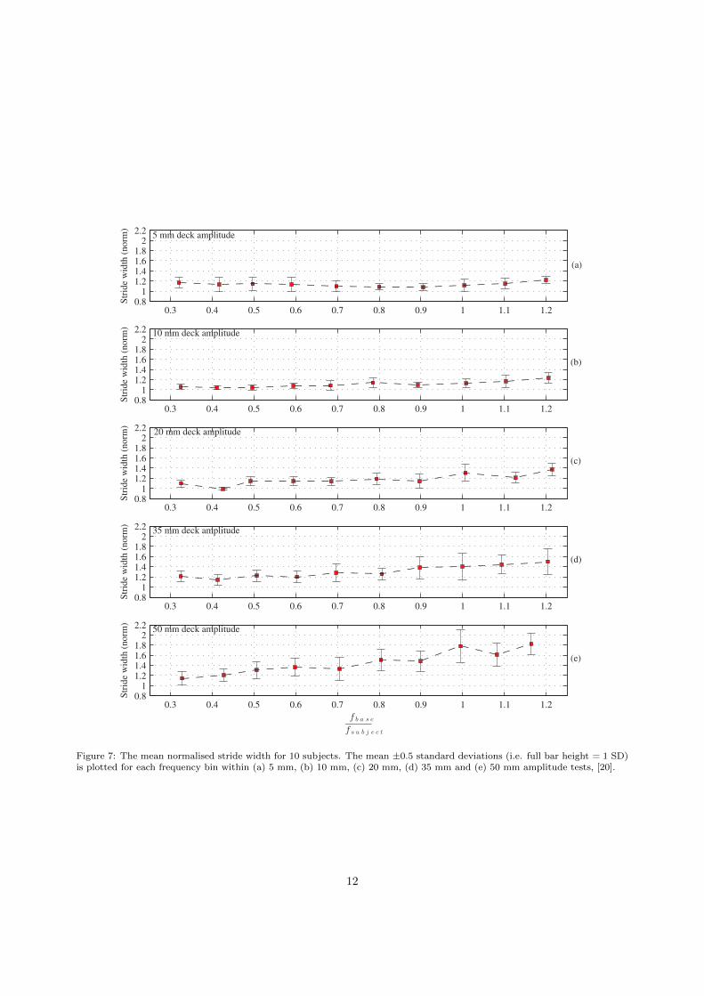
These analyses have been repeated for the remaining 9 subjects and average values of MD, Fig. 6 andnormalised mean stride width, Fig. 7, have been determined. The data has been sorted into frequency binsarranged as follows: Bins = [(0.25 - 0.35), (0.36 - 0.45), (0.46 - 0.55), (0.56 - 0.65), (0.66 - 0.75), (0.76 -0.85), (0.86 - 0.95), (0.96 - 1.05), (1.06 - 1.15), (1.16 - 1.25)] Hz. The mean and standard deviation of datapoints in each bin was then determined. The mean frequency ratio in each bin is used to determine thex-axis position of each data point in Figs. 6 and 7.
The population average data for MD is in agreement with that presented for subject 1. For 5 mmamplitude tests, MD is approximately 20 % with very little inter-subject variability. However as deckacceleration amplitude increases, so too does MD. The tendency for stride widths to stabilise at a constantvalue and therefore reduce MD during synchronisation is also visible in the population data. Figure 7 alsoclearly demonstrated the tendency for mean stride width to increase with deck displacement amplitude
10

0.3 0.4 0.5 0.6 0.7 0.8 0.9 1 1.1 1.20
10203040506070
Modula
tion d
epth
(%
)
0.3 0.4 0.5 0.6 0.7 0.8 0.9 1 1.1 1.20
10203040506070
Modula
tion d
epth
(%
)
0.3 0.4 0.5 0.6 0.7 0.8 0.9 1 1.1 1.20
10203040506070
Modula
tion d
epth
(%
)
0.3 0.4 0.5 0.6 0.7 0.8 0.9 1 1.1 1.20
10203040506070
Modula
tion d
epth
(%
)
0.3 0.4 0.5 0.6 0.7 0.8 0.9 1 1.1 1.20
10203040506070
Modula
tion d
epth
(%
)
f b a s e
f s u b j e c t
10 mm deck amplitude
20 mm deck amplitude
50 mm deck amplitude
5 mm deck amplitude
35 mm deck amplitude
(a)
(b)
(c)
(d)
(e)
Figure 6: The percentage MD for 10 subjects. The mean ±0.5 standard deviations (i.e. full bar height = 1 SD) is plotted foreach frequency bin within (a) 5 mm, (b) 10 mm, (c) 20 mm, (d) 35 mm and (e) 50 mm amplitude tests, [20].
and frequency. This behaviour is conveniently visualised by plotting normalised stride width against deckvelocity amplitude, Fig. 8. In doing so, an approximately linear relationship is identified. Despite inter-subject variability increasing as deck acceleration amplitude grows, it is reasonable to conclude that thebiomechanical behaviour identified in figures 3 and 4 is representative of the test population’s response tolateral base motion.
To investigate the frequency of stride width modulation, the modulation frequency ratio, β, is definedas the ratio of modulation frequency observed to that predicted by the the base oscillation and forcingfrequency relationship, |fbase − fsubject|:
β =Observed modulation frequency
|fbase − fsubject|(4)
11
0.3 0.4 0.5 0.6 0.7 0.8 0.9 1 1.1 1.20.8
11.21.41.61.8
22.2
Str
ide
wid
th (
norm
)
0.3 0.4 0.5 0.6 0.7 0.8 0.9 1 1.1 1.20.8
11.21.41.61.8
22.2
Str
ide
wid
th (
norm
)
0.3 0.4 0.5 0.6 0.7 0.8 0.9 1 1.1 1.20.8
11.21.41.61.8
22.2
Str
ide
wid
th (
norm
)
0.3 0.4 0.5 0.6 0.7 0.8 0.9 1 1.1 1.20.8
11.21.41.61.8
22.2
Str
ide
wid
th (
norm
)
0.3 0.4 0.5 0.6 0.7 0.8 0.9 1 1.1 1.20.8
11.21.41.61.8
22.2
Str
ide
wid
th (
norm
)
f b a s e
f s u b j e c t
(a)
(b)
(c)
(d)
(e)
10 mm deck amplitude
20 mm deck amplitude
35 mm deck amplitude
50 mm deck amplitude
5 mm deck amplitude
Figure 7: The mean normalised stride width for 10 subjects. The mean ±0.5 standard deviations (i.e. full bar height = 1 SD)is plotted for each frequency bin within (a) 5 mm, (b) 10 mm, (c) 20 mm, (d) 35 mm and (e) 50 mm amplitude tests, [20].
12

0 0.05 0.1 0.15 0.2 0.25 0.3 0.350.9
1
1.1
1.2
1.3
1.4
1.5
1.6
1.7
Peak deck velocity (m/s)
Str
ide
Wid
th (
norm
)
Stride Width (norm) = 1.71*(Peak deck velocity) + 1.03
Experimental Data Linear Fit
Figure 8: The mean normalised stride width plotted against peak deck velocity, identifying an approximately linear relationship.
If β = 1 across the full test matrix, it can be concluded that the experimental modulation frequency isgiven by the expression |fbase−fsubject| and is therefore a direct result of the frequency relationship betweenlateral forcing and deck oscillation frequencies. One can therefore logically conclude that the previouslydescribed motivation for stride width modulation (to maintain lateral stability) is consistent across all tests,rather than being a chance observation in the tests selected for discussion.
Figure 9 show the ratio β calculated for each test completed by subject 1. Note that β values for whichfbase ≈ f subject have been omitted as the parameter is not applicable under this frequency regime.
It can be seen that in the majority of cases β ≈ 1, indicating that periodic stride width modulation isgenerally occurring at a frequency equal to |fbase − fsubject|. The biomechanical motivation for alterationof foot position has been identified as being a response to a sinusoidally varying inertia force. Furthermore,the frequency of the SE force harmonic is also identified as fsubject ± |fbase − fsubject|. Therefore, Fig. 9, inwhich β is predominantly equal to one, establishes the link between pedestrian balance behaviour and thegeneration of a SE force harmonic.
Note that for the lowest frequency test during 5 mm and 10 mm amplitude oscillations, plots (a) and(b) in Fig. 9, β ≈ 0. This is due to the stride width modulation not being sufficiently well defined for adominant harmonic to be extracted. In both cases the peak lateral acceleration experienced by the subject< 0.04m/s
2and resulted in negligible influence on stride width. However as the strength of external stimulus
grows, periodic modulation is quickly established. Although not shown here, the same trend (β ≈ 1) wasdemonstrated for all subjects who took part in the campaign.
Figures 5 to 9 demonstrate that the detailed discussion presented in relation to figures 3 and 4 de-scribes typical gait behaviour for the test population. While the underling mechanism at the core of lateralhuman-structure interaction have been identified, the significance of inter-subject variability must also beacknowledged. All subjects exhibit stride width modulation in response to deck motion, however the degreeto which individuals are influenced and therefore the strength of the interaction show large inter-subjectvariability. Therefore there is much work to be done identifying and correlating key parameters with quan-titative measures of the interaction mechanism.
5. The inverted pendulum model of frontal plane balance
The work of Macdonald [10], itself a development of Barker’s earlier work, [21], has motivated a number ofresearchers [14, 15, 22] to pursue a biomechanics-centric analysis of HSI. This approach typically utilises theinverted pendulum (IP) as a means of approximating human frontal plane CoM motion during locomotion,Fig. 10. Application of this simple biomechanical model, stabilised via active control of support or footplacement has produced promising results thus far. However, there are some outstanding uncertainties
13

0.3 0.4 0.5 0.6 0.7 0.8 0.9 1 1.1 1.20
0.5
1
1.5
2
Fre
quen
cy r
atio
, β
0.3 0.4 0.5 0.6 0.7 0.8 0.9 1 1.1 1.20
0.5
1
1.5
2
Fre
quen
cy r
atio
, β
0.3 0.4 0.5 0.6 0.7 0.8 0.9 1 1.1 1.20
0.5
1
1.5
2
Fre
quen
cy r
atio
, β
0.3 0.4 0.5 0.6 0.7 0.8 0.9 1 1.1 1.20
0.5
1
1.5
2
Fre
quen
cy r
atio
, β
0.3 0.4 0.5 0.6 0.7 0.8 0.9 1 1.1 1.20
0.5
1
1.5
2
Fre
quen
cy r
atio
, β
f b a s e
f s u b j e c t
5 mm deck amplitude
10 mm deck amplitude
20 mm deck amplitude
35 mm deck amplitude
50 mm deck amplitude
(a)
(b)
(c)
(d)
(e)
Figure 9: The ratio of observed stride width modulation frequency to that predicted by the expression, |fbase− fsubject|. Datashown for 5 mm (a), 10 mm (b), 20 mm (c), 35 mm (d) and 50 mm (e) amplitude tests, completed by test subject 1, [20].
regarding its suitability for the specific case of walking on a laterally oscillating structure. The aim of thefollowing analysis is to address this uncertainty.
The IP model is well established in the biomechanics field [23]. The model, coupled with the balance lawproposed in [11] can be considered a semi-active model by virtue of the fact that discrete balance correctionsare made at the time of support placement; the so-called foot placement balance strategy. While simulatingthe single stance phase, motion of the pendulum mass is defined solely by its initial conditions and passivemechanics. If one considers walking on a stationary surface, foot placement has been shown to be themain balance strategy, with minor corrections provided by rotation of the upper body about the supportingankle and hip [12]. Therefore the semi-active inverted pendulum model stabilised through foot placementis suitable.
Walking on a laterally moving bridge is fundamentally different from walking on stationary ground. In
14

Figure 10: Inverted pendulum supported on a structure free to move laterally, indicated by coordinate U . The coordinate ymapproximates the lateral or frontal plane motion of a human during the single stance gait phase. The lateral distance betweenpendulum mass and support positions is denoted by u while the pendulum length is Lp, [20].
this case a pedestrian must decide where to place their foot based only on the sensory information they haveat the instant the foot is placed. However, during the single stance phase the bridge continues to oscillate,providing additional sensory stimulus potentially altering the feeling or sense of stability.
On this basis it is logical to hypothesise that external perturbations imposed by a swaying bridge may becorrected for through some form of active control implemented during the single stance phase. Essentially,pedestrians may alter their CoM motion in response to a continuously changing lateral inertia force, in orderto maintain stability. The CoM motion observed while subjects walked on the laterally oscillating treadmillprovide a benchmark against which to compare IP model predictions. The objective is thus to determineif the passive dynamics of the IP model are sufficient to describe human CoM motion while walking on anoscillating deck, or if some form of active motion control should also be implemented.
Lateral acceleration of the IP is approximated by the linearised equation of motion,
ym = −U + ω2u (5)
where U is the lateral acceleration of the supporting structure, ω is the natural frequency of an equivalenthanging pendulum and u is the lateral eccentricity of the pendulum root with reference to the pendulummass [10]. By ensuring that the pendulum support is placed at a sufficient eccentricity u, for each step, a
15

stable gait is simulated. The eccentricity of the support is obtained from the expression,
u ≥ ym,0
ω± bmin (6)
where ym,0 is the pendulum velocity at the time the IP support is placed and bmin is an additional
stability margin, the sign of which alternates on successive steps [11, 12]. The quantity ym + ym
ω is defined asthe extrapolated CoM or XCoM as it considers the extrapolated trajectory of the CoM based on its currentvelocity. For a further discussion of the simulation process, the reader is referred to [10].
5.1. Pendulum versus subject CoM motion: stationary deck
A comparison between observed subject behaviour and model output is now considered. Analysis ofdata relating to subject number 4 is discussed before summary data for the full test population is presented.To facilitate the comparison, an IP model corresponding to the subject in question was established. Thependulum length was determined as the vertical distance to the subject’s CoM (based on marker data andde Leva’s model [19]), while the IP mass was equal to the subject’s body mass. The pendulum was firsttuned to match the subject’s observed behaviour during a stationary test in which no treadmill oscillationwas imposed. Pendulum initial position and velocity were chosen to match that of the subject’s CoM at thebeginning of the comparison. To estimate the initial pendulum support position, a constant medial offsetof 35 mm was applied to the lateral position of the foot-mounted markers. This approximates the averageposition of the subject’s centre of pressure (CoP).
In order to further tune IP behaviour to the subject, the minimum stability margin, bmin from Eq. (6)was used as a tuning parameter. The cumulative area under the (absolute) GRF time history was comparedfor the IP and subject. The areas were compared based on a signal comparison lasting approximately 18 s.bmin was then altered until the difference in areas was a minimum. The final value selected for bmin in thecase presented below was 0.026 m resulting in an area difference of 1.1 %. Figure 11 shows the result of thistuning process for CoM position, velocity and acceleration, plots (a) to (c). Plot (d) shows a comparisonbetween XCoM and CoP position for the subject and IP.
The initial drift in IP trajectory results from a discrepancy between the IP and subject’s initial CoPposition. This results from the approximation of CoP position outlined above. The influence of this discrep-ancy is dissipated within the first two steps and has no bearing on the comparison thereafter. The meanvalue of both time-histories (determined after the first two steps have occurred) has been removed fromboth sets of data in plot (a). This removes the influence of the initial drift in simulated CoM motion. Thesame offsets have also been removed from the simulated and observed data in plot (d). The remaining driftin IP position seen in plot (a) results from small variations in IP step duration, matching the intra-subjectvariability exhibited in the experimental data.
Considering the CoM position, velocity and acceleration comparisons in plots (a), (b) and (c), the IPappears to simulate the CoM trajectory quite well, particularly in the case of the CoM velocity, plot (b).With reference to plot (a), it is apparent that the IP model is unable to simulate ‘atypical’ CoM oscillationssuch as arise from the subject drifting across the treadmill deck as they walk. Nevertheless, the generalcharacter of the simulated oscillatory behaviour is in good agreement with that experimentally observed.The CoM accelerations in plot (c) show good amplitude agreement (ensured by the bmin tuning process),although the subject’s acceleration during the mid-stance deviates significantly from the smooth trajectorysimulated by the IP.
From this comparison it is apparent that both the low and high frequency content of the CoM motion isnot recreated by the IP model. This can be seen, for low frequency content, in plot (a) in which the driftingof the subject’s CoM is not captured by the model. Inability to simulate high frequency content can be seenin plot (c) in which the subject’s CoM acceleration shows high frequency motion during the single stancephase. This low and high frequency motion has a negligible impact on the generation of SE forces, discussedin section 4; as such, it can be considered only a minor deficiency in the model.
Plotting the simulated versus observed behaviour for position, velocity and acceleration data, the cor-relation coefficient (CC) is used as a quantitative measure of the linearity between simulated and observed
16

2 4 6 8 10 12 14 16 18-0.1
-0.05
0
0.05
0.1
Dis
p (
m)
IP Subject
2 4 6 8 10 12 14 16 18
-0.2
0
0.2
0.4
Vel
oci
ty (
m/s
)
2 4 6 8 10 12 14 16 18-0.2
-0.1
0
0.1
0.2
Time (s)
Dis
p (
m)
subject XCoM subject CoP IP XCoM IP CoP2 4 6 8 10 12 14 16 18
-1
0
1
2
Acc
eler
atio
n (
m/s
2)
(a)
(b)
(c)
(d)
Figure 11: Comparison between subject and equivalent IP, (a) CoM position (correlation coefficient, CC = 0.55, slope of thelinear regression line, mreg= 0.51), (b) CoM velocity (CC/mreg = 0.93/0.77), (c) CoM acceleration (CC/mreg = 0.81/0.66) and(d) XCoM and CoP position. A constant medial offset of 35 mm has been applied to the recorded foot position to approximatethe average position of the subject’s CoP [20].
behaviour. In this way, linearity is used as the measure of similarity. These were calculated as 0.55, 0.93and 0.81 for position, velocity and acceleration respectively. This parameter is independent of any scalingdifference between simulated and observed trajectories. This is quantified by the slope of the line of linearregression, mreg, between observed and simulated behaviour. These are calculated as 0.51, 0.77 and 0.66,all identifying that the magnitude of position, velocity and acceleration is underestimated by the IP model.
Plot (d) shows the XCoM and CoP positions for the subject and IP. Note that the subject’s CoP wasapproximated as described above. Again, with the exception of anomalous steps, eg. at t = [3, 5, 13] s, theIP approximates the subject’s behaviour well. Considering the complexity of human locomotion and thecomparative simplicity of the biomechanical model, the general agreement seen in Fig. 11 is, in the authorsopinion, remarkable.
17

5.2. Pendulum versus subject CoM motion: oscillating deck
Having tuned the IP model to the specific subject under consideration, the comparison is now repeatedfor dynamic tests (while employing the same value of the tuning parameter bmin). If the model performs well,it can be concluded that a passive IP is sufficient to describe CoM motion and its continued use is justified.Assessing how well the IP model approximates the subject’s behaviour under these dynamic conditions isessential if the model is to be applied with confidence in the simulation of crowd-induced vibration. Whatfollows in figures 12, 13 and 14 is a selection of dynamic test comparisons which indicate typical IP modelperformance. In all four cases the subject’s lateral forcing frequency was approximately 0.9 Hz.
In order to determine IP support placement, Eq. (6) requires the pendulum velocity at the time ofsupport placement, ym,0. When the IP is supported on a moving deck, there are two possible velocitiesthat may be used within the balance law, velocity relative to the moving deck or velocity measured in aglobal stationary reference frame. With reference to Figs. 12 to 14, when determining the IP supportplacement position from Eq. (6), the CoM velocity relative to the moving deck was found to provide theclosest approximation of subject behaviour.
Figure 12 represents the IP/subject comparison during lateral oscillations of 5 mm amplitude at a fre-quency of 0.3 Hz, the lowest magnitude acceleration imposed. Despite the low acceleration magnitude(0.018m/s
2), there is an immediate widening of the subject’s gait which is not predicted by the CoP place-
ment law, Fig. 12 (d). This is accompanied by larger amplitude CoM oscillations, plot (a), with a corre-sponding increase in velocity and acceleration amplitude, plots (b) and (c). This abrupt change in subjectstride width, initially identified in Fig. 8, is surprising considering the relatively low magnitude of deckmotion imposed. The CCs were determined as 0.49, 0.95 and 0.86 for position, velocity and accelerationrespectively. These values are broadly in line with the static test, however the disparity between observationand simulation is confirmed by the mreg values, 0.41 (pos), 0.57 (vel) and 0.54 (acc). These parametersreveal that the visually reduced agreement results from scaling differences due to the subject’s wider gait,rather than any fundamentally different oscillatory behaviour. Indeed, the CCs for velocity and accelerationare marginally higher than those obtained during the static test
Figure 13 shows the comparison during lateral oscillations of 10 mm amplitude at a frequency of 0.5 Hz.The passive dynamics of the IP appear to predict reasonably well the subject’s oscillatory behaviour in theface of this strengthening stimulus. This is particularly the case between 4s <= t <= 12s, during whichposition, velocity and acceleration are well predicted. However atypical behaviour, eg. between 13s <=t <= 14s obviously cannot be predicted by the IP. The correlation and regression data was calculated asCC/mreg = 0.64/0.34 (pos), 0.93/0.66 (vel) and 0.81/0.59 (acc). Both velocity and acceleration comparisonshow similar parameter values to the tests discussed previously, however the position CC is noticeablyimproved, although significantly underestimated in terms of amplitude.
It can be postulated that the strengthening external stimulus leads to a convergence in simulated andobserved CoM motion, i.e. the stronger the equivalent inertia force experienced by the subject, the morelike a passive IP they behave during the single stance phase. It is at least reasonable to suggest that thepassive nature of the IP model is sufficient to describe the subject’s CoM oscillation in the presence of lateralbase motion. That is to say the addition of a further active control element on CoM does not appear to bewarranted. While active balance control certainly plays a role in maintaining stability during locomotionon a laterally oscillating deck, the CoM behaviour is adequately described by the dynamics of a passive IP.
It is worth commenting on the IP performance in the case when the lateral forcing and deck oscillationfrequencies coincide. This case is shown in Fig. 14, in which the oscillation amplitude and frequency are20 mm and 0.9 Hz respectively. Exceptionally good agreement is observed between the subject and IPbehaviour, quantified by the correlation and regression data, CC/mreg = 0.89/0.78 (pos), 0.97/0.93 (vel)and 0.88/0.89 (acc).
As mentioned in relation to Fig. 4, there is a constant phase relationship between the lateral forcingand deck oscillation frequencies. As a result the equivalent inertia force imposed on the subject and IP, atthe time of support placement, remains constant from gait cycle to gait cycle and there is no modulation ofstride width. In this particular case, the CoP position is well predicted by the balance law, Eq. (6), and as aresult the CoM position, velocity and acceleration are also well predicted. Not withstanding the inaccuracy
18

2 4 6 8 10 12 14 16 18-0.15
-0.1
-0.05
0
0.05
0.1
0.15
Dis
p (
m)
IP Subject
2 4 6 8 10 12 14 16 18-0.4
-0.2
0
0.2
0.4
Vel
oci
ty (
m/s
)
2 4 6 8 10 12 14 16 18
-0.2
-0.1
0
0.1
0.2
Time (s)
Dis
p (
m)
subject XCoM subject CoP IP XCoM IP CoP
2 4 6 8 10 12 14 16 18-2
-1
0
1
2
Acc
eler
atio
n (
m/s
2)
(a)
(d)
(b)
(c)
Figure 12: Comparison between subject and equivalent IP, deck oscillation 5 mm amplitude at 0.3 Hz. (a) CoM position(CC/mreg = 0.49/0.41), (b) CoM velocity (CC/mreg = 0.95/0.57), (c) CoM acceleration (CC/mreg = 0.86/0.54) and (d)XCoM and CoP position. A constant medial offset of 35 mm has been applied to the recorded foot position to approximatethe average position of the subject’s CoP [20].
of support placement position, exemplified in Figs. 12 and 13, Fig. 14 further confirms the suitability of apassive model for CoM oscillatory behaviour.
A limitation of the CoP placement law becomes apparent as the magnitude of deck velocity experiencedby the IP grows. According to Eq. (6), the eccentricity of the CoP contains a term proportional to CoMvelocity, y0
ω , and the additional stability margin, bmin.In the event that the IP and deck have global velocities in the same direction but the deck velocity
magnitude is greater than the absolute velocity of the IP, the velocity of the IP relative to the deck will be inthe medial direction. As a result, the term y0
ω will be opposite in sign to bmin. As deck velocity magnitude
increases, bmin is effectively eroded by y0
ω and a ‘crossover’ step occurs. A crossover step describes thesituation in which the IP CoP is placed on the ‘wrong’ side of the CoM for the imminent step. Figure15 shows the IP/subject comparison for deck oscillation amplitude and frequency, 35 mm at 0.6 Hz. Theoccurrence of crossover steps can be seen in plot (d). This behaviour, although ensuring IP stability, signalsthe breakdown of the balance law as the IP behaviour no longer resembles human locomotion. For this
19

2 4 6 8 10 12 14 16 18-0.15
-0.1
-0.05
0
0.05
0.1
Dis
p (
m)
IP Subject
2 4 6 8 10 12 14 16 18-0.4
-0.2
0
0.2
0.4
Vel
oci
ty (
m/s
)
2 4 6 8 10 12 14 16 18
-0.2
-0.1
0
0.1
0.2
Time (s)
Dis
p (
m)
subject XCoM subject CoP IP XCoM IP CoP
2 4 6 8 10 12 14 16 18-2
-1
0
1
2
Acc
eler
atio
n (
m/s
2)
(d)
(c)
(b)
(a)
Figure 13: Comparison between subject and equivalent IP, deck oscillation 10 mm amplitude at 0.5 Hz. (a) CoM position(CC/mreg = 0.64/0.34), (b) CoM velocity (CC/mreg = 0.93/0.66), (c) CoM acceleration (CC/mreg = 0.81/0.59) and (d)XCoM and CoP position. A constant medial offset of 35 mm has been applied to the recorded foot position to approximatethe average position of the subject’s CoP [20].
reason, comparisons have not been presented for 35 mm and 50 mm amplitude tests.
5.3. Pendulum versus subject CoM motion: population data
Before the subject/IP comparison can be further investigated, the issue of velocity reference frame mustbe briefly addressed. As mentioned above, there is a level of uncertainty regarding which reference frameis most appropriate for each comparison test. For example, when focusing on a fixed reference point in thelaboratory, the subject may have perceived their CoM velocity in the global reference frame. However whenlooking down at their feet moving relative to the treadmill deck (or the horizontal stabilising bar), theymay have perceived velocity in the local reference frame. This leads to difficulty when trying to generaliseIP/subject comparison data for the full population. Therefore the approach adopted here will be to presentanalyses based on local and global reference frames, in parallel. It can then be assumed that the subject’sactual RF during testing lay on or between these two boundaries, an imperfect but practical approach.
Comparisons between each subject and their equivalent IP have been carried out for all 10 subjects.
20

2 4 6 8 10 12 14 16 18-0.15
-0.1
-0.05
0
0.05
0.1
0.15
Dis
p (
m)
IP Subject
2 4 6 8 10 12 14 16 18-0.6
-0.4
-0.2
0
0.2
0.4
0.6
Vel
oci
ty (
m/s
)
2 4 6 8 10 12 14 16 18-0.3
-0.2
-0.1
0
0.1
0.2
0.3
Time (s)
Dis
p (
m)
subject XCoM subject CoP IP XCoM IP CoP
2 4 6 8 10 12 14 16 18
-2
-1
0
1
2
Acc
eler
atio
n (
m/s
2)
(a)
(b)
(c)
(d)
Figure 14: Comparison between subject and equivalent IP, deck oscillation 20 mm amplitude at 0.9 Hz. (a) CoM position(CC/mreg = 0.89/0.78), (b) CoM velocity (CC/mreg = 0.97/0.93), (c) CoM acceleration (CC/mreg = 0.88/0.89) and (d)XCoM and CoP position A constant medial offset of 35 mm has been applied to the recorded foot position to approximate theaverage position of the subject’s CoP [20].
All comparison data, for all subjects has been combined for 5mm, 10mm and 20mm amplitude tests andsimulated versus observed CoM motion plotted. The correlation and regression data for both local and globalvelocity simulations is summarised in table 3. This values of CC and mreg obtained for the full populationconfirm the generality of the previous discussion in relation to figures 12, 13 and 14. CoM velocity andacceleration are predicted more accurately than position in terms of both linearity and magnitude. This islargely due to the fact that the velocity and acceleration data is zero-centred and does not contain the driftingvisible in the position data. With the exception of CoM velocity and acceleration during 10 mm amplitudedeck oscillations (based on local velocity simulations), the IP underestimates CoM motion magnitude in allcases. When averaged over the test population, there appears to be negligible difference between local andglobal simulation predictions. This is not surprising as any variation in CoM motion induced by a change ofperception reference frame is likely to be subtle and may change several times during the course of a singletest observation. Nevertheless, table 3 confirms the suitability of a passive IP model for CoM motion in thefrontal plane.
21

2 4 6 8 10 12 14 16 18-0.2
-0.15-0.1
-0.050
0.050.1
0.150.2
Dis
p (
m)
IP Subject
2 4 6 8 10 12 14 16 18-0.6
-0.4
-0.2
0
0.2
0.4
0.6
Vel
oci
ty (
m/s
)
2 4 6 8 10 12 14 16 18-0.3
-0.2
-0.1
0
0.1
0.2
0.3
Time (s)
Dis
p (
m)
subject XCoM subject CoP IP XCoM IP CoP2 4 6 8 10 12 14 16 18
-3
-2
-1
0
1
2
3
Acc
eler
atio
n (
m/s
2)
(a)
(b)
(c)
(d)
Figure 15: Comparison between subject and equivalent IP, deck oscillation 35 mm amplitude at 0.6 Hz demonstrating theoccurrence of crossover steps. (a) CoM position, (b) CoM velocity, (c) CoM acceleration and (d) XCoM and CoP position Aconstant medial offset of 35 mm has been applied to the recorded foot position to approximate the average position of thesubject’s CoP, [20].
Table 3: Comparison between subject and equivalent IP CoM motion. Correlation (CC) and regression (mreg) parametershave been determined for the full test population. Comparisons derived from IP simulations based on local and global IP CoMvelocity are indicated separately [20].
5 mm 10 mm 20 mmCC mreg CC mreg CC mreg
CoM positionLocal 0.48 0.36 0.45 0.56 0.58 0.68Global 0.47 0.34 0.40 0.46 0.52 0.43
CoM velocityLocal 0.94 0.86 0.93 1.09 0.88 0.91Global 0.95 0.86 0.92 0.92 0.87 0.69
CoM accelerationLocal 0.87 0.83 0.87 1.04 0.84 0.89Global 0.88 0.83 0.86 0.91 0.85 0.72
22

6. Conclusions
In this paper, an analysis of subject balance behaviour while walking on both a stationary and laterallyoscillating treadmill is presented. The aim of this work has been (i) to obtain a better understanding ofthe root cause or source of the SE GRF, identified in Fig. 3 (d) and (ii) to assess the suitability of thepassive IP model for the specific case of walking on a laterally oscillating deck. The approach taken in thisinvestigation was to investigate the behaviour of a relatively small number of subjects, but in greater detailthan has typically been the case in the literature thus far.
It has been confirmed that the interaction forces arise directly as a result of the foot placement position,which itself is a function of pedestrian stability. The frequency of stride width modulation was confirmed asthe modulus of the difference between the lateral forcing and deck oscillation frequencies. The underlyingreason for this was revealed by examining the subject’s CoM oscillation and recognising the influence of asinusoidally varying inertia force induced by deck motion. Furthermore, the degree to which the subjectalters their gait is determined by the degree to which their frontal plane stability is impaired by deckmotion. Thus the link between frontal plane balance behaviour and generation of the SE component of thelateral GRF has been established. Although there is a large degree of ISV, the fundamental HSI mechanismidentified, namely periodic stride width modulation resulting in amplitude modulation of the GRF, can beconsidered typical for the full test population.
The additional stimulus provided by deck motion has also been shown to cause an increase in meanstride width when compared with walking on a stationary deck. A linear relationship was found betweenthe normalised stride width and deck velocity amplitude. This balance response was exhibited for even thesmallest deck oscillation amplitudes imposed in this study.
The experimental observations and analysis presented herein reveal that the IP model, stabilised on astep-by-step basis, is at least qualitatively sound; that is to say the IP model combined with the CoP place-ment law proposed in [11], generates self-excited forces through the alteration of CoP placement position; aprocess analogous to amplitude modulation. Examination of actual subject balance behaviour has revealedthe same mechanism at work. The IP stability law does not however account for the increase in mean stridewidth demonstrated by subjects walking on an oscillating structure.
Furthermore, the single stance oscillatory behaviour of subjects walking on the laterally oscillating deckhas been found to be well described by a passive IP model for the range of amplitudes ≤ 20 mm andfrequencies ≤ 1.1 Hz. The magnitude of lateral acceleration experienced on full scale structures, includingthat experienced at the onset of lateral instability, will almost certainly be within this range. Thus theworking hypothesis which suggests the need for active balance control during the single stance phase hasbeen disproven. While active balance control based on sensory feedback is certainly utilised in stabilisinglocomotion on an oscillating structure, its influence on single stance CoM oscillation can be neglected infavour of the passive IP.
In summary, when one considers the need for simulation accuracy and efficiency, on balance, the SDoFpassive IP, stabilised by CoP placement, performs remarkably well. More accuracy in CoP placement maybe achieved by implementing additional active control elements. However, the potential benefit of thisimproved accuracy must be balanced against the increased complexity introduced. For the purposes ofsimulating lateral HSI, the IP/control law system in its current form is judged appropriate and sufficient forimplementation as a biomechanical model of frontal plane CoM motion.
References
[1] P. Dziuba, G. Grillaud, O. Flamand, S. Sanquier, Y. Tetard, La Passerelle Solferino comportement dynamique (dynamicbehaviour of the Solferino Bridge), Bulletin Ouvrages Metalliques 1 (2001) 34–57.
[2] S. Nakamura, Field measurements of lateral vibration on a pedestrian suspension bridge, The Structural Engineer 81(2003) 22–6.
[3] A. Ronnquist, Pedestrian induced lateral vibrations of slender footbridges, Ph.D. thesis, Norwegian University of Scienceand Technology (2005).
[4] J. M. W. Brownjohn, P. Fok, M. Roche, P. Omenzetter, Long span steel pedestrian bridge at Singapore Changi Airport -part 2: Crowd loading tests and vibration mitigation measures, The Structural Engineer 82 (2004) 28–34.
[5] J. H. G. Macdonald, Pedestrian-induced vibrations of the Clifton Suspension Bridge, uk, Proceedings of the ICE - BridgeEngineering 161 (2008) 69–77.
[6] P. Dallard, A. J. Fitzpatrick, A. Flint, S. Le Bourva, A. Low, R. M. Ridsdill Smith, M. Willford, The London MillenniumFootbridge, The Structural Engineer 79 (2001) 17–33.
23

[7] F. Ricciardelli, A. D. Pizzimenti, Lateral walking-induced forces on footbridges, Journal of Bridge Engineering 6 (2007)677–688.
[8] E. T. Ingolfsson, C. T. Georgakis, F. Ricciardelli, J. Jonsson, Experimental identification of pedestrian-induced lateralforces on footbridges, Journal of Sound and Vibration 330 (2011) 1265–1284.
[9] S. P. Carroll, J. S. Owen, M. F. M. Hussein, Reproduction of lateral ground reaction forces from visual marker data andanalysis of balance response while walking on a laterally oscillating deck, Engineering Structures 49 (2013) 1034–47.
[10] J. H. G. Macdonald, Lateral excitation of bridges by balancing pedestrians, Proceedings of the Royal Society a-Mathematical Physical and Engineering Sciences 465 (2009) 1055–1073.
[11] A. L. Hof, M. G. J. Gazendam, W. E. Sinke, The condition for dynamic stability, Journal of Biomechanics 38 (2005) 1–8.[12] A. L. Hof, R. M. van Bockel, T. Schoppen, K. Postema, Control of lateral balance in walking: Experimental findings in
normal subjects and above-knee amputees, Gait & Posture 25 (2007) 250–258.[13] A. L. Hof, S. Vermerris, W. Gjaltema, Balance response to lateral perturbations in human treadmill walking, The Journal
of Experimental Biology 213 (2010) 2655–2664.[14] S. P. Carroll, J. S. Owen, M. F. M. Hussein, Crowd-bridge interaction by combining biomechanical and discrete element
models, in: Proceedings of the 8th international conference on structural dynamics, Leuven, 2011.[15] M. Bocian, J. H. G. Macdonald, J. F. Burn, Biomechanically inspired modelling of pedestrian-induced forces on laterally
oscillating structures, Journal of Sound and Vibration 331 (2012) 3914–3929.[16] S. P. Carroll, J. S. Owen, M. F. M. Hussein, A coupled biomechanical/discrete element crowd model of crowd-bridge
dynamic interaction & application to the Clifton Suspension Bridge, Engineering Structures 49 (2013) 58–75.[17] Charnwood Dynamics Ltd., Leicestershire, UK, Coda mpx30 User Guide, Charnwood Dynamics Ltd, Leicestershire, UK.[18] V. M. Zatsiorsky, V. N. Seluyanov, L. G. Chugunova, Contemporary Problems of Biomechanics, CRC Press, Massachusetts,
1990, Ch. Methods of determining mass-inertial characteristics of human-body segments, pp. 272–291.[19] P. de Leva, Adjustment to zatsiorsky-seluyanov’s segment inertia parameters, Journal of Biomechanics 29 (1996) 1223–
1230.[20] S. P. Carroll, Crowd-induced lateral bridge vibration, Ph.D. thesis, Faculty of Engineering, University of Nottingham
(2013).[21] C. Barker, Some observations on the nature of the mechanism that drives the self-excited lateral response of footbridges.,
in: Proceedings of the 1st International conference; design and dynamic behaviour of footbridges, Paris, 2002.[22] F. A. McRobie, Long-term solutions of Macdonald’s model for pedestrian-induced lateral forces, Journal of Sound and
Vibration 332 (2013) 2846–2855.[23] M. Townsend, Biped gait stabilization via foot placement, Journal of Biomechanics 18 (1985) 21–38.
24