carsharing fleet location design with mixed vehicle types...

Carsharing Fleet Location Design with Mixed Vehicle Types for

CO2 Emission ReductionJoy Chang

Joint work with Siqian Shen (U of Michigan IOE)and Ming Xu (U of Michigan SNRE)

INFORMS Annual Meeting NashvilleNovember 13, 2016

1

Outline

• Introduction

• Mathematical Models

• Computational Results

• Conclusions

2

What is carsharing?

• Short-term car rentals

• One-way or round-trip

3

Industry growth

4

346,610

670,762

1,251,504

0

200000

400000

600000

800000

1000000

1200000

1400000

2006 2008 2010

Worldwide membership tripled over 4 years

South America Australia Asia Europe North America Worldwide

11,501

19,403

32,665

0

5000

10000

15000

20000

25000

30000

35000

2006 2008 2010

Worldwide fleet sizes tripled over 4 years

South America Australia Asia Europe North America Worldwide

Adapted from “Carsharing and personal vehicle services: worldwide market developments and emerging trends”, S.A. Saheen.

Carsharing providers

5

Private companies Nonprofit Government

Entity Zipcar City CarShare Seattle

Vehicles removed (foregone buying or sold)

15 privately owned vehicles for every Zipcar

17,000 1,200 – 1,600

Reduced vehicle miles

90% of members drive 5,500 less miles

140 million miles N/A

Carshare design and optimization

• Consider strategic decisions• Car types to purchase to appeal to larger customer base? • Carbon emissions limit?

• Evaluate the impact• Case study (Zipcar Boston)• Mathematical modeling

• Optimize profitability and quality of service via models that• Incorporate round-trip and one-way demands• Incorporate carbon emissions constraint• Make strategic decisions about diverse portfolio of vehicle types

6

Outline

• Introduction



• Conclusions

7

Framing the problem

Carsharing companies need a diverse vehicle portfolio

How does demand for different vehicle types affect:

• Profitability

• Quality of service

• One-way and round-trip

• Denied trip

• Trip fulfillment

• Purchasing decisions

• Carbon emissions

8

Building the spatial-temporal network

• Example: • Zones 1, 2

• Time periods 0, 1, 2, 3

• nit: Zone i at time t

9

Round-trip arcs




Type Volume Origin Destination Start End

One-way 3 2 1 0 3

Round-trip 2 2 2 3

10

One-way arcs





One-way 3 2 1 0 3

Round-trip 2 2 2 3

11

Idle arcs





One-way 3 2 1 0 3

Round-trip 2 2 2 3

12

Relocation arcs





One-way 3 2 1 0 3

Round-trip 2 2 2 3

13

Final spatial-temporal network





One-way 3 2 1 0 3

Round-trip 2 2 2 3

14

Defining Model 1

Inputs

• Car purchase cost and emissions generated

• Car rental price

• Arc capacity (demand)

Objective

• Maximize total revenue of operating cars over set time

15

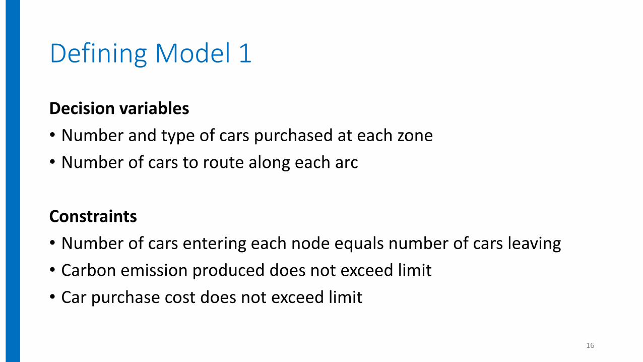
Defining Model 1

Decision variables

• Number and type of cars purchased at each zone

• Number of cars to route along each arc

Constraints

• Number of cars entering each node equals number of cars leaving

• Carbon emission produced does not exceed limit

• Car purchase cost does not exceed limit

16

Assumptions

• A set of service zones and a finite number of service periods

• Serve one-way and round-trip rentals

• Cars can be relocated, to balance vehicle distributions

• Unsatisfied demand is immediately lost

17

Network arc parameters

18


19


20


21

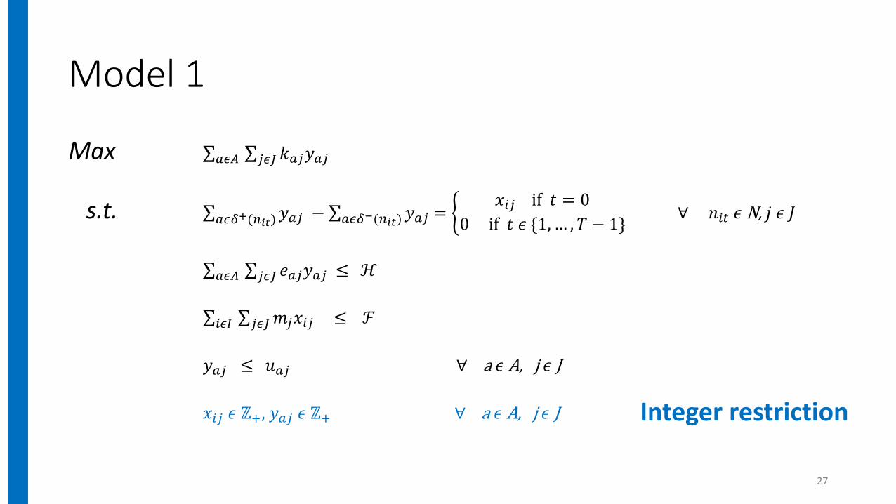
Model 1

Max σ𝑎𝜖𝐴 σ𝑗𝜖𝐽 𝑘𝑎𝑗𝑦𝑎𝑗

s.t. σ𝑎𝜖𝛿+(𝑛𝑖𝑡) 𝑦𝑎𝑗 − σ𝑎𝜖𝛿−(𝑛𝑖𝑡) 𝑦𝑎𝑗 = ቊ𝑥𝑖𝑗 if 𝑡 = 0

0 if 𝑡 𝜖 {1, … , 𝑇 − 1}∀ 𝑛𝑖𝑡 𝜖 N, 𝑗 𝜖 𝐽

σ𝑎𝜖𝐴 σ𝑗𝜖𝐽 𝑒𝑎𝑗𝑦𝑎𝑗 ≤ ℋ

σ𝑖𝜖𝐼 σ𝑗𝜖𝐽 𝑚𝑗𝑥𝑖𝑗 ≤ ℱ

𝑦𝑎𝑗 ≤ 𝑢𝑎𝑗 ∀ a 𝜖 A, j 𝜖 J

𝑥𝑖𝑗 𝜖 ℤ+, 𝑦𝑎𝑗 𝜖 ℤ+ ∀ a 𝜖 A, j 𝜖 J

22

Maximize total revenue

Model 1



0 if 𝑡 𝜖 {1, … , 𝑇 − 1}∀ 𝑛𝑖𝑡 𝜖 N, 𝑗 𝜖 𝐽





23

Flow balance constraint

Model 1



0 if 𝑡 𝜖 {1, … , 𝑇 − 1}∀ 𝑛𝑖𝑡 𝜖 N, 𝑗 𝜖 𝐽





24

Budget limit

Model 1



0 if 𝑡 𝜖 {1, … , 𝑇 − 1}∀ 𝑛𝑖𝑡 𝜖 N, 𝑗 𝜖 𝐽





25

Carbon emissions limit

Model 1



0 if 𝑡 𝜖 {1, … , 𝑇 − 1}∀ 𝑛𝑖𝑡 𝜖 N, 𝑗 𝜖 𝐽





26

Capacity constraint

Model 1



0 if 𝑡 𝜖 {1, … , 𝑇 − 1}∀ 𝑛𝑖𝑡 𝜖 N, 𝑗 𝜖 𝐽





27

Integer restriction

Extension to Model 1 (Model 2)

• First-come first-serve (FCFS) principle:

If there is a car available (idle) at that node when a customer comes in, you must serve the customer

• Model 2 (M2) enforces FCFS

• Denied trip percentage serves as metric

• New binary variable introduced at each node

28


29

Add the following constraints to M1:

𝑦(𝑛𝑖𝑡 ,𝑛𝑖,𝑡+1),𝑗 ≤ 𝑣𝑗𝑚𝑎𝑥𝑧𝑖𝑡

𝑗∀ i 𝜖 I, t = 0, 1, …, T – 1, j 𝜖 J

σ𝑎𝜖𝛿+(𝑛𝑖𝑡)∪(𝐴𝑂∩𝐴𝑈)(𝑢𝑎𝑗 − 𝑦𝑎𝑗) ≤ 𝑣𝑗

𝑚𝑎𝑥(1 − 𝑧𝑖𝑡𝑗

) ∀ i 𝜖 I, t = 0, 1, …, T – 1, j 𝜖 J

𝑧𝑖𝑡𝑗

𝜖 {0, 1} ∀ i 𝜖 I, t = 0, 1, …, T – 1, j 𝜖 J


30



𝑗∀ i 𝜖 I, t = 0, 1, …, T – 1, j 𝜖 J



) ∀ i 𝜖 I, t = 0, 1, …, T – 1, j 𝜖 J

𝑧𝑖𝑡𝑗

𝜖 {0, 1} ∀ i 𝜖 I, t = 0, 1, …, T – 1, j 𝜖 J

If 𝑧𝑖𝑡𝑗

is 1, then idle cars can flow from that node.

Else, no idle cars can flow from that node.


31



𝑗∀ i 𝜖 I, t = 0, 1, …, T – 1, j 𝜖 J



) ∀ i 𝜖 I, t = 0, 1, …, T – 1, j 𝜖 J

𝑧𝑖𝑡𝑗

𝜖 {0, 1} ∀ i 𝜖 I, t = 0, 1, …, T – 1, j 𝜖 J

If 𝑧𝑖𝑡𝑗

is 1 (idle cars can flow from that node), then all capacity must be fulfilled.


32



𝑗∀ i 𝜖 I, t = 0, 1, …, T – 1, j 𝜖 J



) ∀ i 𝜖 I, t = 0, 1, …, T – 1, j 𝜖 J

𝑧𝑖𝑡𝑗

𝜖 {0, 1} ∀ i 𝜖 I, t = 0, 1, …, T – 1, j 𝜖 J

All capacity must be fulfilled to have idle cars flow from the node.

Outline

• Introduction



• Conclusions

33

Data description• Zipcar operations for Greater Boston

• Timeframe from Oct. 1 to Nov. 30, 2014

• # of reservations made each hour for 60 zip codes

34

Car type description

• 4 sedan types

• Gasoline powered, electric, hybrid, plug-in hybrid electric

35

Computational efficiency

• Tests run for M1 and M2

• Vary one-way demand

• M1 significantly faster than M2*Use Python + Gurobi 6.0.3, Intel(R) Core(TM) i5-4200U CPU with 6GM RAM

36

Carbon emissions constraint• Vary carbon emission constraint between 3 x 106 and 6 x 106 grams

• Demand: 40% LX, 20% Hybrid, 20% PHEV, 20% EV

37

Gasoline-powered

Carbon emissions constraint• Vary carbon emission constraint between 3 x 106 and 6 x 106 grams

• Demand: 40% LX, 20% Hybrid, 20% PHEV, 20% EV

38

Non-gasolinepowered

Quality of Service (QoS)

• Vary one-way proportion between 0%, 40%, 80%, 100%

• M1 enforces high QoS and FCFS principle

• Deny trip percentage between 0.1% and 1%

39





40





41

Trip fulfillment for 40% one-way setting

42

Capacity

Trip fulfillment for 40% one-way setting

43

Capacity

Trips taken

Outline

• Introduction



• Conclusions

44

Conclusions

Carsharing companies want to• Expand market demographic

• Provide reliable service

• Benefit environment by lowering carbon emissions

Our model • Determines diverse vehicle portfolio

• Enforces high QoS and first-come first-serve principle

• Enforces carbon emissions constraints while still maximizing profit

45

The future: service-based transportation

• Ford’s expanded business plan is to be “both an auto and a mobility company”

• General Motors invested $500 million in Lyft, a ridesharing service

• Future work:

Developing more strategies to expand ridesharing services

Integrating shared autonomous vehicles into daily life

46

Questions?

47

carsharing fleet location design with mixed vehicle types...

Documents