CAS for Physics Examples

Electrostatics, Magnetism, Circuits and

Mechanics of Charged Particles Part 1

Vector- and Scalar Fields

Electric Field

Leon Magiera and Josef Böhm

Contents

Introduction 3

I Vector and Scalar Fields 4

II Electric Field 15

3

Introduction

This text is devoted to solving practical problems in the field of electricity and magnetism

using computer algebra systems (CAS). The problems described usually appear in the programs of standard General Physics courses at university level (engineering and science). Some of them would also be suitable for high schools.

Maxima is a powerful tool for the manipulation of symbolic and numerical expressions, including differentiation, integration, vectors, matrices, . . . and so on. It also provides commands for plotting functions, curves and data in two and three dimensions. We chose Maxima because it is a free software package. It can be downloaded from its website,

http://maxima.sourceforge.net, where documentation in several languages can also be found.

The use of Maxima significantly reduces the computational work and allows a student (or teacher) to concentrate on physical ideas (which is most important), rather than on the very time consuming technical side - performing the derivations by hand.

For a first try of Maxima, you may wish to try the examples in First Steps with Maxima. Please don't understand this paper as a complete introduction in working with Maxima. Maxima-experts will certainly find ways to solve some problems in another way. Maxima is much more powerful that it is shown here. You can produce complex programs, your own libraries and much more.

Leon Magiera is physicist at the Wroclaw University of Science and Technology, Josef Böhm is a retired school teacher and founder of the International DERIVE and CAS-TI User Group. His work was putting all parts together in a common form and adding DERIVE and TI-NspireCAS treatments of some examples. DERIVE is off the market since several years but still widely used all over the world. DERIVE and TI-NspireCAS are running up to the latest operations systems. The DERIVE and TI-NspireCAS parts can be distinguished by another font set.

the Authors

All files are available on request.

We welcome any comments and suggestions regarding this book. You may contact us via e-mail at:

leon.magiera@wp.pl nojo.boehm@pgv.at In preparation:

2nd part: Magnetic Field 3rd part: Circuits 4th part: Mechanics of Charged Particles

For DERIVE User Group information goto www.austromath.at/dug/

4

I. Vector and Scalar Fields

Vector and scalar fields are very important concepts in physics. They are just respectively a vector and a scalar functions of space variable. Some differential operators are defined acting on those functions, which are in common use in physics, like: gradient, divergence, rotation and Laplacian.

We start with definitions using Cartesian coordinates x, y, z.

The Gradient of a scalar function is the vector

gradx y z

, , . I.1

The Divergence of the vector field A A A Ax y z , , is a scalar of the form

divAA

x

A

y

A

zx y z

. I.2

The Curl of the vector field A A A Ax y z , , is the following vector field

xyx AAAzyx

kji

Acurl

. I.3

The Laplacian of a scalar function is a scalar of the form

2

2

2

2

2

2x y z . I.4

Now we try to solve some problems:

I.1 Calculate the following expressions:

a) the gradient of the function 1

( ) ,rr

b) ( ),div r

c) ( ),r

divr

d) 1

,div gradr

e) ( ),curl r

where r is the modulus of the position vector ),,( zyxr

,

5

Solutions:

We need loading the library "vector":

Note that result %o5 can be rewritten in a simple concise form:

3( ) .

rgrad r

r

Some problems are too difficult for a computer program. The next example is too hard for many computer algebra systems. Maxima – and DERIVE as well – returns:

This is the DERIVE result:

Remark: The above result is not correct. The correct result is proportional to the Dirac -function

δ(r). Unfortunately, many computer algebra systems we tried did not return the correct result.

6

My last attempt was "asking" MATHEMATICA (www.wolframalpha.com) and see the answers:

Input in another form delivers the -function, great.

Exercise: Show that the divergence of the vector field of the form ,c r

r

with c an arbitrary constant

equal zero.

■▬▬▬▬▬▬▬▬

I.2 Prove the identity 3 3

,a r a r

grad curlr r

where a

is an arbitrary, constant vector.

( , , )r r x y z

is a position vector and r denotes its modulus.

Solution:

We add the definition of a

(which is a_) and use the “~”-character as operation sign for the vector

product. We show that the difference of both sides simplifies to the zero vector.

7

It is remarkable that the DERIVE proof is much shorter and much more elegant (two ways):

Michel Beaudin from ETS Montreal produced a fine vector analysis library for TI-NspireCAS (https://cours.etsmtl.ca/seg/mbeaudin/documents/Kit_ETS_MB.tns) which allows performing the proof in one single line:

é■▬▬▬▬▬▬▬▬

I.3 Prove the identity ( ( )) ( ( )) ,curl curl a grad div a a

where

( ( , , ), ( , , ), ( , , ))x y za a a x y z a x y z a x y z

is a differentiable vector. The symbol Δ denotes the

Laplace operator 2 2 2

2 2 2.

x y y

Solution:

The identity can be rewritten in the equivalent form

( ( )) ( ( )) [0,0,0].curl curl a grad div a a

Exercise: a

and ( ( , , ), ( , , ), ( , , ))x y zb b b x y z b x y z b x y z

are arbitrary differentiable vectors and

f = f(x,y,z) and g= g(x,y,z) are arbitrary differentiable functions.

Prove the following identities:

a) curl(grad(f)) = [0,0,0]

b) ( ) ( ) ( ) [0,0,0],grad f g f grad g g grad f

c) ( ( ) 0,div curl a

d) ( ) ( ),div a b b curl a a curl b

e) ( ) ( ) ( ),div f a f div a a grad f

f) ( ) ( ) ( ) .curl f a f curl a grad f a

8

We will demonstrate two of the exercises from above, a) and f):

a)

That's not fine. Both packages deliver different results. We know that the curl should be a vector. To be on the safe side, let's ask another CAS:

Although TI-NspireCAS does not simplify the partial derivatives we see that we obtain the zero vector. DERIVE gives the correct answer.

f)

■▬▬▬▬▬▬▬▬

In more advanced textbooks cross product and curl in the Cartesian coordinate system may be written using Levi-Civita tensor ijk . This tensor is defined as )( kjiijk eee

(i,j,k = 1,2,3), where

, ( 1 2 3)ie i , ,

are the unit vectors

]1 ,0 ,0[ ],0 ,1 ,0[ ],0 ,0 ,1[ 321 eee

. . Using this notation, the components of the cross product of the vectors

1 2 3 1 2 3[ , , ] [ , , ], [ , , ] [ , , ]x y z x y zA A A A A A A B B B B B B B

can be written as follows

( ) i ijk j kj k

A B A B

(i=1,2,3).

9

The components of the curl of B B B B [ , , ]1 2 3 are given by

,( ) ijk k jij k

curl B B

, (i=1,2,3)

where ,k jB is the partial derivative of the k-th component of vector B

with respect to the j-th

variable. For example 3,2zB

By

.

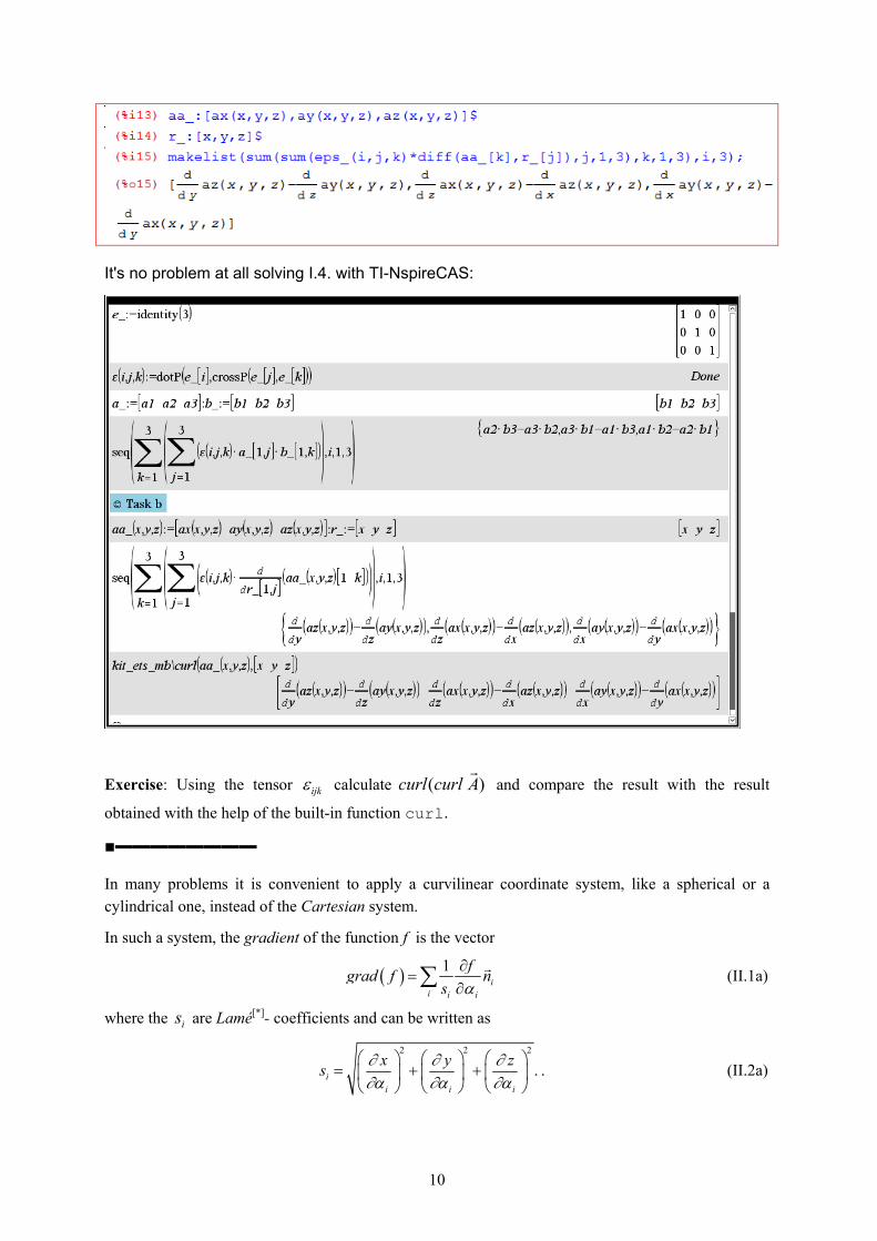
I.4. Using the definitions above calculate:

a) the components of the cross product of the following vectors:

[ , , ], [ , , ]x y z x y zA A A A B B B B

,

b) the components of the curl of the vector

[ ( , , ), ( , , ), ( , , )]x y zA A x y z A x y z A x y x

.

Solution:

We enter the unit vectors collected in an identity matrix and the Levi-Civita tensor:

%o7 is not correct. Why that? Further investigation shows that the vector product v v

results in 0

instead of the zero vector.

What to do? Easy enough: define your own cross product!

Now it is correct. We proceed with problem b):

10

It's no problem at all solving I.4. with TI-NspireCAS:

Exercise: Using the tensor ijk calculate ) ( Acurlcurl

and compare the result with the result

obtained with the help of the built-in function curl.

■▬▬▬▬▬▬▬▬ In many problems it is convenient to apply a curvilinear coordinate system, like a spherical or a cylindrical one, instead of the Cartesian system.

In such a system, the gradient of the function f is the vector

1i

i i i

fgrad f n

s

(II.1a)

where the si are Lamé[*]- coefficients and can be written as

2 2 2

.ii i i

x y zs

. (II.2a)

11

x, y, z are the Cartesian coordinates and

1 2 3( , , )

denote curvilinear coordinates and in

denote the local unit vectors.

The divergence of the vector field A A A A( , , )1 2 3 is the following scalar quantity

divAs s s

s s A s s A s s A

1

1 2 3

2 3 1

1

1 3 2

2

1 2 3

3

( ) ( ) ( ) (II.3a)

The curl of a vector field A A A A( , , )1 2 3 is of the form

31 2

2 3 1 3 1 2

1 2 3

1 1 2 2 3 3

nn n

s s s s s s

curl A

s A s A s A

(II.4a)

The Laplacian of the function f may be written as

2 3 1 3 1 2

3 31 1 2 2

1 2 3 1 2 3

1

s s s s s s ff fss s

fs s s

(II.5a)

To solve the next problems we will use the definitions from above, as well as the built-functions of the computer algebra systems.

[1] Gabriel Lamé, French mathematician 1795-1870. Well known is the Lamé-Curve 1n n

x y

a b

which

with n>1 is also called "super ellipse".

■▬▬▬▬▬▬▬▬

12

I.5. Determine the gradient of the generic function f(r,θ,φ) defined in spherical coordinates.

Solution:

We enter the Cartesian and the spherical coordinates and the relations between them, followed by

the definition of the Lamé coefficients. Applying trigreduce on I.1a gives the gradient – but

not in its most comfortable form. The second component can be rewritten as ( , , )

.sin( )

df r

dr

DERIVE enables the same procedure. It is not necessary to manipulate the result in order to obtain the final result. DERIVE offers a second – much shorter – method using an extended GRAD-function:

spherical is the coordinate geometry matrix with the independent variables in the first row and the corresponding Lamé coefficients in the second one.

Comment: In case of the right-hand coordinate system, in which the positive z-axis is

associated with the north pole, the colatitude is measured in radians south from the north

pole and colongitude is measured in radians east from the positive x-axis. In the DERIVE

function the angles and have the reverse meaning. It means that is replaced by and

by , which can be seen when we compare results %o7 (wxMaxima) and #2 (DERIVE).

13

Let's have a look on the TI-NspireCAS screen:

Exercise: First generate the geometry matrices for Cartesian, spherical and cylindrical coordinates and then write a generalized function for calculating the gradient for all systems.

■▬▬▬▬▬▬▬▬

14

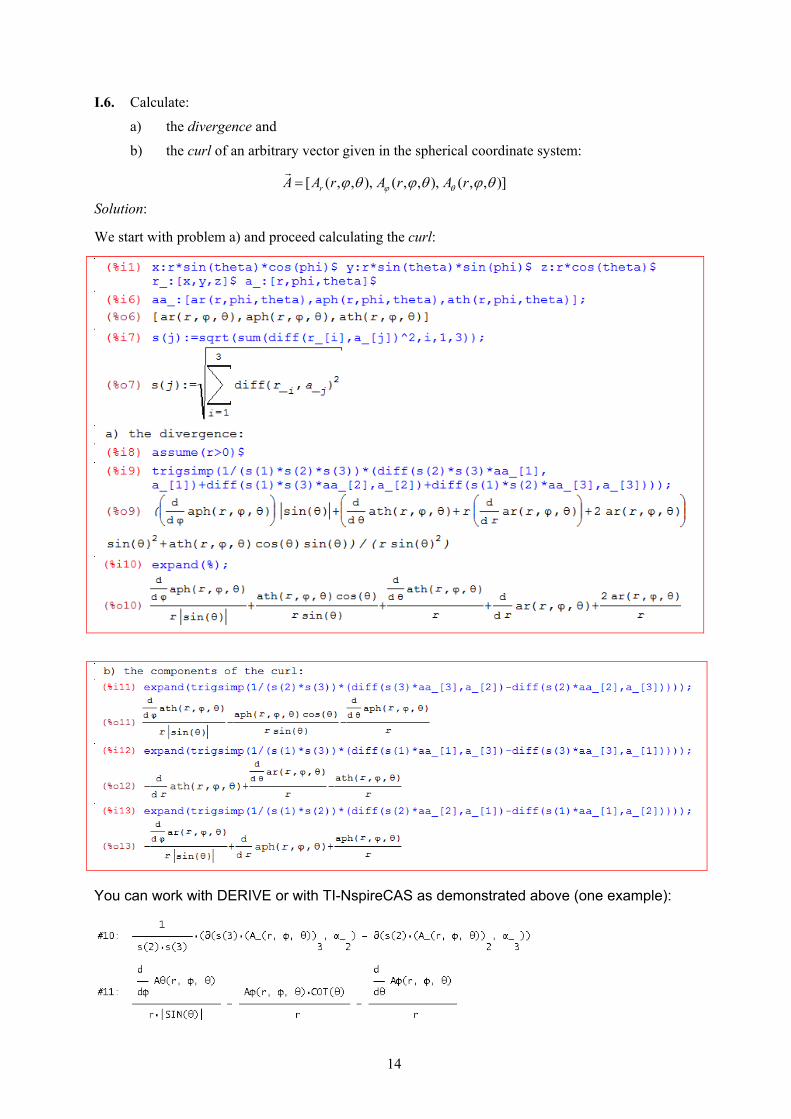
I.6. Calculate:

a) the divergence and

b) the curl of an arbitrary vector given in the spherical coordinate system:

[ ( , , ), ( , , ), ( , , )]rA A r A r A r

Solution:

We start with problem a) and proceed calculating the curl:

You can work with DERIVE or with TI-NspireCAS as demonstrated above (one example):

15

Exercise: Calculate the divergence of an arbitrary vector in cylindrical coordinates.

[ ( , , ), ( , , ), ( , , )].r zA A r z A r z A r z

■▬▬▬▬▬▬▬▬

I.7. Find the expression for the Laplacian of the function Φ(r, φ, θ) in spherical coordinates.

Solution:

We enter definition (I.5a) in a more concise form:

3

31

3 21

1

( )1( , , )

( )( )

k

i i i

j

s kf r

s is j

We can compare with the DERIVE result (consider that φ and θ are interchanged!):

Exercise: Find the Laplacian of function f(r,φ,z) in cylindrical coordinates.

16

II. Electric Field

Introduction

The most elementary part of physics dealing with electromagnetic interactions is called electrostatics. Electrostatics describes the interaction between stationary electric charges. The force

of interaction between two point charges obeys Coulomb’s law. Force F

acting on a charge q

whose position is ,r due to a charge Q at ,R

is given by

F

qQ

r Rr R

14 0

3( ) ,

where o denotes the permittivity in a vacuum.

Electrostatic interactions may also be described in a different way, by means of the concept of

an electric field. Within this formalism, the force F

acting on a charge q is the product of the

charge q and the electric field E

caused by the charge Q

,F q E

hence

30

1( ) .

4

F QE r R

q r R

The modern formulation of electrostatics is based on Gauss's law*, which may be written in the form

0

,S

QE dS

where Q is the total charge giving rise to the electrostatic field E

, confined by a closed surface S. In differential notation Gauss's law is of the form

0

,div E

where is the charge density.

One very important property of an electrostatic field is the fact that it can be described by a scalar function called the potential. This is a consequence of conservative nature of electrostatic

force. Field intensity E

and potential are related to each other by the equation

( ).E grad

(*) https://en.wikipedia.org/wiki/Gauss's_law

17

Thus, Gauss's law, expressed in terms of the potential, reads

2

0

,

which is known as Poisson's law ( 2 denotes the Laplace operator).

The electric field created by a system of electric charges is the vector sum of the fields created by the individual charges (the principle of superposition).

Using the equations given above, we can solve standard exercises as presented below. Some of them will deal with discrete charges, the other ones with continuously distributed charges.

PROBLEMS

II.1 Split point charge Q into two point charges q and (Q – q), separated by a distance of d, so that the force of interaction between them is maximum.

Solution: According to Coulomb's law, the magnitude of the force of repulsion between the charges is given by

and

The problem can also be solved by directly finding the maximum value of the function F (even its nominator only) i.e. by solving the equation

( ) 0.d

q Q qdq

Let’s find the solution of the above equation

and then check the kind of the turning point by evaluating the second derivative for the obtained solution

From %o3 and %o5 we see that at q = Q/2 the interactive force is maximum.

Note: In the above exercise evaluation of sign function is not necessary. See below

18

We will skip the DERIVE and the TI-NspireCAS treatment as well because we recognize the quadratic function with zeros at q1 = 0 and q2 = Q. As the graph is a downwards open parabola its vertex is at q0 = Q/2.

■▬▬▬▬▬▬▬▬ II.2 We consider a system of an infinite number of point charges Q, which are distributed on a

half-line in such a way that the first charge is put at a distance of d from the beginning of the

half-line, A, and each successive distance is chosen to be as times greater than the previous

one. Find the force acting on a point charge q placed at A.

Solution: The resultant force acting on q is the algebraic sum of Coulomb forces originating from the successive charges Q.

Let’s try to evaluate the above expression.

The above sum was calculated with i.e. the force takes the simple form for

For we get

Let us notice that in our series (geometrical series) the ratio 2

1

appears.

19

Hence the solution of our problem (This is the DERIVE solution:

With TI-NspireCAS we cannot distinguish between lower and uppercase characters, so we denote Q as qq:

II.3 Three stationary charges 321 and , QQQ are placed at the following positions 1 1 1 1( , , z ),R x y

2 2 2 2 3 3 3 3( , , z ) and ( , , z )R x y R x y

, respectively.

a) Write down expressions describing the field potential at the point ( , , ).r x y z

b) Compute the resultant force acting on an electron of charge q for the data:

x= 6m, y= –7m, z= 9m, 1 2 34 , 3 , 0.5Q C Q C Q C ,

1 2 3(0, 2, 0), ( 3,2,0) and (0,0,0)R R R

.

20

Solution: The potential at the point ,r

due to a single charge Qj placed at the point given by the position

vector jR

can be expressed as

4

1

0 j

jj

Rr

Q

According to the principle of superposition, the resultant potential is

j

j ,

a) To make the notation more concise the components of the position vectors jR

of the charges

jQ are entered in the form of the matrix R_.

while the charges as components of the vector Q_.

Then the resultant potential at ( , , )r x y z

can be written as follows:

with

21

b) The desired force has the form

F F F

where

gradEEqF

,

We load the file “vect” and enter the above relations.

The magnitude of the resultant force is

We import the value of the electron charge and electric constant from the utility file

“physical_constants”.

In the next step we evaluate the magnitude of the resultant force at the point [6m, 7m,9m]r

.

In the final step we replace symbol “.” by ”*”.

Simplifying units returns

Next page shows the respective DERIVE session followed by the TI-NspireCAS screens:

22

  TI-NspireCAS treatment is following. The gradient function is not provided by the system, so we use Michel Beaudin's library (presented in DNL#98) in order to apply his grad function. Elementary charge q and electric constant (permittivity in a vacuum) ε0 are provided among

the “Constants” in the “Unit Conversions” which can be found in the Documents Toolbox.

 

 

23

 ■▬▬▬▬▬▬▬▬

 II.4 Three point charges Q1, Q2, Q3 are placed as shown in Fig II.4 .

Fig II.4

a) Give the formula for the resulting electric field in a generic point ( , , ).r x y z

b) Calculate all Cartesian components of the electric field on the x-axis.

c) For identical charge (Q1 = Q2 = Q3 = Q) and the distances x1 = x2 = y1 = y3 = b calculate

the parameter 2y

b for which the field component Ey of the resultant field

disappears at x = 0.

d) Plot the curve Ey(x) for the calculated parameter η.

Solution:

a) First we enter the given data:

24

According to the principle of superposition (page 16), the resultant field at the point r

can be expressed as

b) We calculate all Cartesian components of electric field along the x-axis:

c) We extract the field component Ey:

At the origin of the reference system and for all identical charges and the distances

1 2 1 3 2, x x y y b y b we have

It is desired be equal to zero. To find the parameter it remains to solve the above equation

Hence the desired parameter value is 1

42 .

25

Then the explicit form of Ey is

(d) Now we plot the desired component Ey(x) (for the calculated parameter η value) and the

following remaining parameters values: ε0 = 1, Q = 1, b = 1 (needs loading library "draw").

-0.06

-0.05

-0.04

-0.03

-0.02

-0.01

0

-3 -2 -1 0 1 2 3

Ey(x)

The TI-Nspire treatment follows:

26

It is not necessary to add any restrictions for the variables for solving the equation.

Now we can plot f1(x).

27

■▬▬▬▬▬▬▬▬

II.5 Equal charges of value Q are placed in the vertices of a regular hexagon with sides of length a.

Fig II.5

Calculate:

a) the potential of the field in the centre of the hexagon,

b) the electric field and potential in the centre of one given side of your choice.

Solution:

Remember, the potential of the electric field at the point r

resulting from a charge jQ placed in a

point jR

is described by the relation

j

j

j

Q

r R

1

4 0 ,

In the problem discussed jQ Q , (j=1, 2 ,..., 6). Hence, the resultant potential can be written in

the form 6 6

1 10 0

1 1= .

4 4j

j jj j

Q Q

r R r R

28

The components of the position vectors jR

, taking the centre of the hexagon as the origin of the

coordinate system, are given by:

acos , asin , 0, ( 1,2,...,6)3 3j j jx j y j z j

We enter the formulae for the position vectors of the charges, the position vector of the observed point and the resultant potential according to the equation from above:

a) Then the potential in the centre of the hexagon is

b) In the centre of any given side the potential is

To calculate the field we enter the well known relation between field and the potential

.E grad

and then we calculate the field in the centre of one side of the hexagon (let's say in the point

0, 3, 02

ax y z

.

DERIVE and TI-NspireCAS treatments are very similar. Exercise: Compute the magnitude of the electric field and potential in the centres of all remaining sides of the hexagon and compare the obtained results.

■▬▬▬▬▬▬▬▬

29

II.6 There are five charges 1 2 3 4 0, , , and Q Q Q Q Q located as shown in Fig. II.6.

Fig. II.6

a) Find the relation between charges 1 2 3 4, , , Q Q Q Q for which the resulting acting on

the charge Q0 disappears?

b) Plot the equipotential curves and the 3D-plot of the potential.

Solution:

One of the solutions, namely: 1 2 3 4 Q Q Q Q (full symmetry) is obvious. We try to find the

remaining solutions.

a) In the problem we have

To find the remaining solutions we take advantage of relations met in the previous task. The

potential of the electric field at the point r

resulting from a charge Qj placed in a point jR

is

described by the relation

Let us apply the connection between potential and field strength and calculate the field strength at

the location point of charge 0.Q

The electric field vector disappears in the desired point if every its component is zero. This implies that we have to solve two equations. We try to solve this equation system e.g. for the unknowns Q1 and Q2.

30

From the received solution we can conclude that the resultant power acting on charge Q0 disappears when conditions Q1 = Q3 and Q2 = Q4 are fulfilled.

Of course, if every component of any vector is equal zero then its value (length of the vector) is equal to zero. We are getting the task to the solution of only one equation

[0,0,0]

0r

EE

.

We try to solve this equation for one unknown e.g. for Q1:

As charges are real we deduce from %o14 that Q2 = Q4 and further Q1 = Q3.

Of course, the same relations between charges are being received by solving the equation with respect to any other charge e.g. Q2 (see above %o15).

We can obtain solution of the problem in a single step applying the solve command:

b) Let's produce the plots:

We generate the 3D-plot of the potential.

31

This is another form of the plot:

The equipotential curves in the xy-plane are plotted:

The two plots below show the DERIVE plots (after similar calculations):

32

The TI-NspireCAS 3D-plot of the potential looks pretty good (left hand side), but unfortunately it is not possible to produce its contour plot.

What we can do to get an impression of the contour lines, is tracing the surface.

See below the trace for z = 0.08 (left) and z = 0.16 (right).

With the symbolic pocket calculator Voyage 200 we can plot the surface and its contour plot as well. The screen shots right and below are demonstrating this. It is understandable that we cannot expect high quality plots like those done on a PC but for a hand held product the plots are pretty good.

■▬▬▬▬▬▬▬▬

33

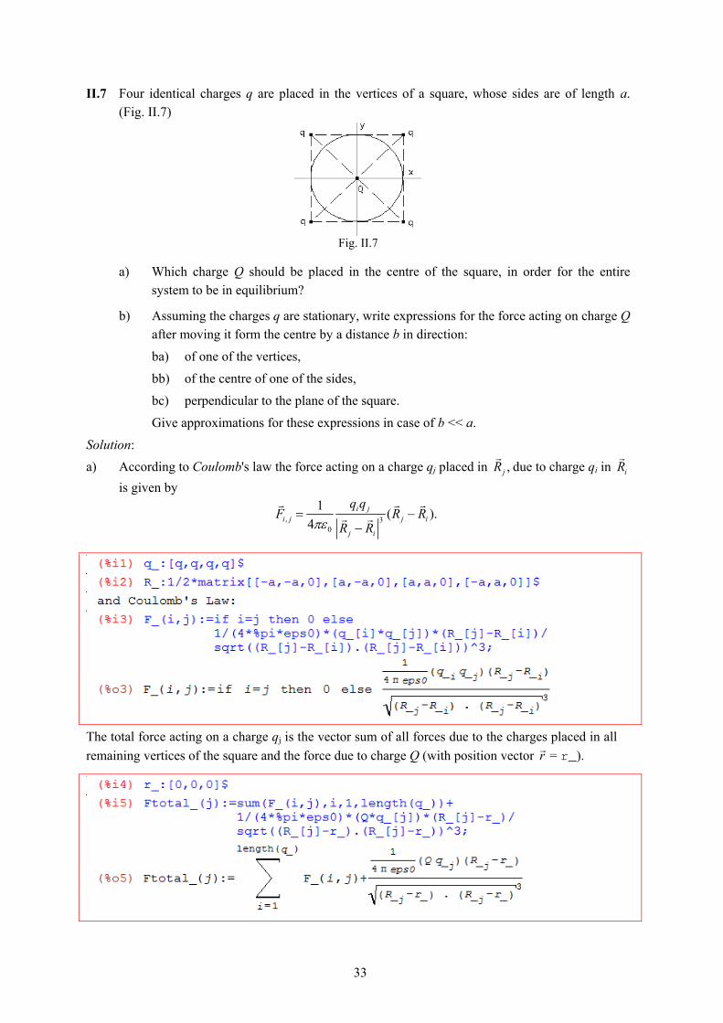
II.7 Four identical charges q are placed in the vertices of a square, whose sides are of length a. (Fig. II.7)

Fig. II.7

a) Which charge Q should be placed in the centre of the square, in order for the entire

system to be in equilibrium?

b) Assuming the charges q are stationary, write expressions for the force acting on charge Q after moving it form the centre by a distance b in direction:

ba) of one of the vertices,

bb) of the centre of one of the sides,

bc) perpendicular to the plane of the square.

Give approximations for these expressions in case of b << a.

Solution:

a) According to Coulomb's law the force acting on a charge qj placed in ,jR

due to charge qi in iR

is given by

, 30

1( ).

4i j

i j j i

j i

q qF R R

R R

The total force acting on a charge qj is the vector sum of all forces due to the charges placed in all

remaining vertices of the square and the force due to charge Q (with position vector r

= r_).

34

The system will be in equilibrium when the resultant force acting on one of the charges q from the other charges equals zero. First we will find the required charge Q for j = 1.

The total force should be zero for all indices j. Let's verify the obtained solution:

b) Now we will calculate the force FQ

arising on charge Q due to its displacement. Q is placed at

position ( , , )r x y z

.

ba) The resulting force acting on charge Q

can be entered in the following form (%i14). For small displacements b << a we will introduce the parameter δ (b = δ a) and then perform the Taylor expansion of force

FQ

= FQ_ up to the first order term.

35

We see that the calculated force is repulsive. Let's calculate the magnitude of this force, too:

bb) Now charge Q moves towards the centre of a side of the square:

For a small displacement we get:

We see that the calculated force is repulsive again.

bc) In the last case we have a displacement in direction perpendicular to the plane of the square (see next figure).

We perform the same procedure as above and we find out that now the resulting force is attractive.

Resuming we see (results %o16, %o19 and %o21) that in point (0,0,0) the equilibrium state of charge Q is an unstable one.

DERIVE and TI-NspireCAS treatment as well are easy to perform and deliver the same results.

■▬▬▬▬▬▬▬▬

36

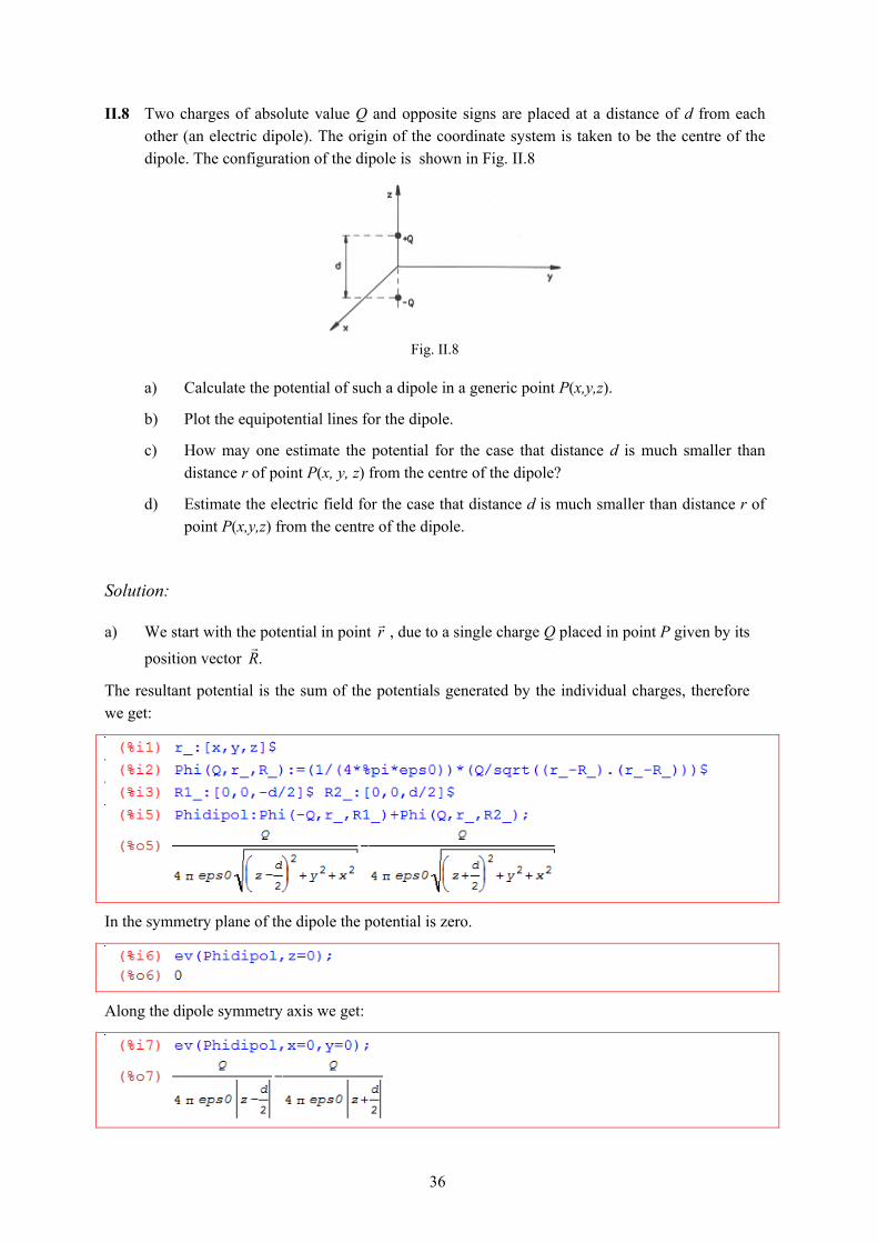
II.8 Two charges of absolute value Q and opposite signs are placed at a distance of d from each other (an electric dipole). The origin of the coordinate system is taken to be the centre of the dipole. The configuration of the dipole is shown in Fig. II.8

Fig. II.8

a) Calculate the potential of such a dipole in a generic point P(x,y,z).

b) Plot the equipotential lines for the dipole.

c) How may one estimate the potential for the case that distance d is much smaller than distance r of point P(x, y, z) from the centre of the dipole?

d) Estimate the electric field for the case that distance d is much smaller than distance r of point P(x,y,z) from the centre of the dipole.

Solution:

a) We start with the potential in point r

, due to a single charge Q placed in point P given by its

position vector .R

The resultant potential is the sum of the potentials generated by the individual charges, therefore we get:

In the symmetry plane of the dipole the potential is zero.

Along the dipole symmetry axis we get:

37

b) Let's plot the equipotential curves in the xz-plane (i.e. for y = 0):

c) In order to estimate the potential of the dipole we use the parameter d

r describing the ratio

of the length of the dipole to the distance of the observed point from the centre of the dipole and then calculate the Taylor expansion of the potential with respect to the parameter δ preserving only the first order term of the expansion. Then we will return to the previous variables.

38

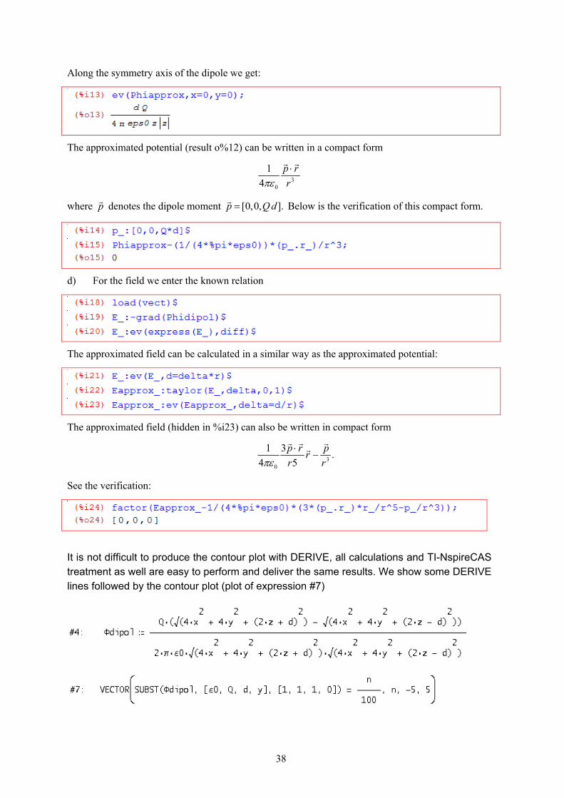
Along the symmetry axis of the dipole we get:

The approximated potential (result o%12) can be written in a compact form

30

1

4

p r

r

where p

denotes the dipole moment [0,0, ].p Q d

Below is the verification of this compact form.

d) For the field we enter the known relation

The approximated field can be calculated in a similar way as the approximated potential:

The approximated field (hidden in %i23) can also be written in compact form

30

1 3.

4 5

p r pr

r r

See the verification:

It is not difficult to produce the contour plot with DERIVE, all calculations and TI-NspireCAS treatment as well are easy to perform and deliver the same results. We show some DERIVE lines followed by the contour plot (plot of expression #7)

39

With TI-Nspire we proceed like in Example II.6: we plot the surface and then trace in y-direction which is upwards in our case (left: y = 0.2, right: y= -0.04).

Exercise: There are three point charges located on a line (linear quadrupole). Plot the equipotential lines and produce a 3D plot of the potential of this quadrupole with charge –q at x = –a, the second charge –q at x = a and the third charge 2q located at the origin of the reference system.

■▬▬▬▬▬▬▬▬

40

II.9 Point charge Q is located at a distance b from the centre of a grounded conducting sphere of radius R (b < R). Find the position and magnitude of an image charge q which generates a zero potential on the spherical surface. Plot the equipotential lines.

Solution:

The potential at a distance r from point charge Q can be expressed as

0

1( , ) .

4

QQ r

r

By symmetry, the image charge must lie on the straight line connecting Q and the centre of the sphere.

Fig. II.9

The potential must be zero on the surface of the sphere. In particular it must be zero in the nearest and farthest points on the equator of the sphere which contains Q. Hence we build two equations and solve the system for a and q.

From %o4 we deduce magnitude q and distance a of the image charge:

Then the potential is

The equipotential lines lie in the xz-plane. They are presented on the next page (ε0 = 1, Q = 1, b = 5, R = 3).

41

There is no problem calculating and plotting with DERIVE:

■▬▬▬▬▬▬▬▬

42

The following problems deal with systems of continuous charge distributions.

II.10 Calculate the electrical field potential and the field intensity vector for the field created by a thin rod of length l with uniform charge density.

Solution: The configuration of the system is shown in Fig. II.10.

Fig. II.10

The field caused at point P(x,y) due to the charge on an infinitesimally small segment of the rod dx is given by

0

1,

4dx

dr

where σ denotes the line charge density, r is the distance of the observed point P from the element dx.

2 2( )r y x x .

The resultant potential is expressed by the following integral:

0 0

1 .

4

l dxr

Then the field intensity is the gradient of the field potential:

.E grad

We transfer these expressions into "Maxima language" and then calculate the potential Φ:

At the symmetry axis of the rod (x = l/2) we get

43

Let' now find the field intensity:

For the axis of symmetry Maxima gives:

For an infinite long rod the field is inverse proportional to the distance from the rod:

It is interesting to perform the calculation from above using another CAS, e.g. DERIVE:

%o4 (Maxima) should be identical with #4 (DERIVE):

44

Identity of %o8 and #5 can be checked easily manually and %o9 #6. What about Φ and its AREA-functions?

The expression for the potential is rather complicated in DERIVE, the expression for the field intensity is complicated in both systems. However, field intensity can take a much

simpler form introducing angles 1 and 2 (see Fig. II.10a).

Fig. II.10a

We can read off: 1 21 2

tan( ) tan( ) , .tan( ) tan( )

d d d db l b

b b l

and

In this case it turns out that the Maxima calculation is more complicated:

But finally we also reach our goal!

45

II.11 Calculate the force of the mutual interaction of two uniformly charged rods of length L1 and L2 lying on the same line and of charge Q1 and Q2 respectively. The distance between the rods is d . (Parameters for the plot: ε0 = 1, Q1 = 1, Q2 = 2, L1 = 0.5, L2 = 1.5)

Solution: We use Coulomb’s law:

L1 L2

dx1 dx2

d

L1 L2

d

The force of interaction between two charged segments of lengths dx1 and dx2 with coordinates x1 and x2 (starting points of the segments) is given by

1 21 22

0 1 2

1

4 ( )dF dx dx

x x

where 21 , are the charge densities of the rods ( 11

1

Q

L , 2

22

Q

L ).

The resultant force is obtained by integration

1 1 2 1 1 2

1 1

1 2 1 22 1 2 12 2

0 2 1 0 1 2 2 10 0

1 1( ) ( )

4 ( ) 4 ( )

L L d L L L d L

L d L d

Q QF dx dx dx dx

x x L L x x

.

We enter the expressions from above and proceed with the integration:

%o5 can be simplified to the compact form:

Fig. II.11

46

Now we can assume parameter values and then plot force F vs distance d:

0.006

0.008

0.01

0.012

0.014

0.016

0.018

2 2.5 3 3.5 4 4.5 5

F(d)

Here are the TI-NspireCAS screens:

47

■▬▬▬▬▬▬▬▬

II.12 A thin electric rod is formed in the shape of an arc, which is a fragment given by the angle 0 of

a circle of Radius R. The rod is uniformly charged with charge Q. Find the vector of the electric field strength for any point z0 along the axis of the circle passing the centre and perpendicular to the plane of the circle. Discuss the result obtained (ε0 = Q = R = 1).

Solution:

Fig. II.12

According to Fig. II.12 the vector of the electric field strength can be calculated using the formula

30

1( , ) ,

4

o

oo

E z r R dr

where 0

Q

l is the charge density with 0 0 ,l R and the vector 0 0(0 ,0 , ) ( , , )r x y z x y z

with x = R cos(), y = R sin(). ( r

is the direction vector from the wire to the point on the axis.)

48

We enter the relations given above and then calculate the field.

Now let us analyze the result obtained: At the centre of the circle (z0 = 0) we get the field:

When the arc turns out to become the full circle (0 = 2π) then only the z-component of field E_ is

nonzero – as should be expected:

We extract the 3rd component of the field and we can easily see (from %o8) that at a large distance (|z0| >> R) the charged circle is equivalent to a point charge.

In infinity the field is zero.

We find the extremal value of the field for the full ring:

The field takes its extreme values in the points 2

0,0, .2

R

We enter the given parameter values and then we can plot the graph of the z-component of the field.

49

-0.03

-0.02

-0.01

0

0.01

0.02

0.03

-10 -5 0 5 10

Ez(z0)

Unfortunately Maxima does not provide such a wonderful tool as sliders for further investigation of the influence of parameters. Most other CAS do. We show the application of sliders to study the influence of charge Q and radius R as well.

Left hand side is a screen shot of DERIVE, right hand side a screen shot of TI-NspireCAS handheld. With TI-NspireCAS we can easily find the turning points, too.

Exercise: Consider two half circles of radii R mutually perpendicular with coinciding centres and uniformly charged with charge Q. Find the vector of the electric field strength and its magnitude in the circles' centre.

Hint: Use solution of problem II.12.

■▬▬▬▬▬▬▬▬

50

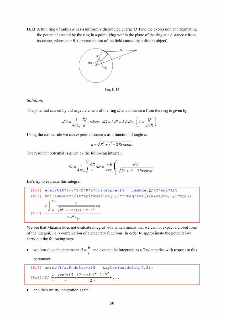
II.13 A thin ring of radius R has a uniformly distributed charge Q. Find the expression approximating the potential created by the ring in a point lying within the plane of the ring at a distance r from its centre, where r>>R. (approximation of the field caused by a distant object).

Fig. II.13

Solution: The potential caused by a charged element of the ring dl at a distance a from the ring is given by

0

1,

4

dQd

a where .

2

QdQ dl R d

R

Using the cosine rule we can express distance a as a function of angle :

2 2 2 cos .a R r Rr

The resultant potential is given by the following integral:

22

2 20 0

0 0

1.

4 4 2 cos

R R dd

a R r Rr

Let's try to evaluate this integral.

We see that Maxima does not evaluate integral %o3 which means that we cannot expect a closed form of the integral, i.e. a combination of elementary functions. In order to approximate the potential we carry out the following steps:

we introduce the parameter R

r and expand the integrand as a Taylor series with respect to this

parameter

and then we try integration again:

51

So we get the final result of the above approximation (%o6). But let us resubstitute for and bring the

result in a neat form (cancelling needs the factor command!).

We can work through the problem with TI-NspireCAS without any problems in the same way (including the cancellation )!

Exercise: Show that the electric field in the considered approximation is identical to the field caused by a point charge.

■▬▬▬▬▬▬▬▬

52

II.14 A circular plate of radius R is uniformly charged with a surface charge density .

a) Calculate the field potential and electric field in a point lying a distance z away from the plate along the axis of symmetry perpendicular to the plate.

b) By applying the appropriate limit calculate the function describing the field intensity resulting from an uniformly charged plate.

c) Find an approximation for the field potential and intensity for the case that the radius of the plate is small with respect to the distance z.

Solution: The sketch of the situation is shown in Fig. II.14.

Fig. II.14

Similar to II.13 the potential resulting from charge Q in a point with distance l from the plate is given by

0

1,

4

dQd

l where 2 2l r z is the distance of charge dQ from the observed point.

dQ = ds is the charge of the surface element of the plate. In polar coordinates ds = r dr d, therefore

we have

.dQ ds r dr d

The potential caused by the plate is given by the integral

2

00

0

.4

R

rdr d

l

Taking into account the relation between field strength and field potential is – in the meanwhile well known – given by

( )E grad

and the symmetry of the problem (only the z-component of the field strength can differ from zero), it is sufficient to calculate this component only:

.z

dE

dz

53

a) We enter the expressions from above and calculate potential and field strength.

b) To get the result for the plane (R ) it is sufficient to calculate the limit of Ez..

c)

Remark: Of course, the electric field caused by a uniformly charged plane can be most easily obtained by applying Gauss' law.

Different methods of calculating the field strength deriving from the plain homogeneously loaded up still exist. We use the estimated electric field originating from the endless bar homogeneously loaded up (problem II.10 expression %o9).

The obtained result has the form 0

,2 d

where λ

denotes the linear charge intensity and d the distance of the point of observation from the bar. We try to use this result for our calculation. For this purpose we will divide the plane in stripes of widths dx.

Fig. II.14a

Charge dQ contained in surface element ds = dx dy is dQ = ds = dx dy. On the other hand

dQ = λ dy.

Comparing these two expressions for dQ we get λ = dx. Therefore in the solved exercise we have

20 0

1

2 2

dx r rdE E dx

r r r

with [ ,0, ].r x z

x

y

54

It is resulting from the symmetry of the problem, that only the z-component of the filed should be nonzero. We will calculate the field and then read off this component:

Let's perform the same calculation with DERIVE:

There we find another output for the third component of the field – and an undefined first component, too.

In fact, calculation of the x-component is not trivial, namely in the calculation procedure

the integral 2 2

.x

dxx z

This integral can be transformed by substitution to the form .du

u

Not each CAS returns the

satisfactory result. For example DERIVE gives "?" which is undefined. Maxima gives 0.

Below we show the calculation of the limit procedure stepwise:

0 0 0 0 0 0lim lim lim ln lim ln lim ln lim ln 0.

a

a a a a a aa

du du du a a a

u u u a

For calculating the field strength from the plain homogeneously loaded up it is possible also to take advantage of the model describing the field strength from the dielectric circular ring homogeneously charged.

Make appropriate calculations. Use the result %o8 of problem II.12.

Fig. II.14b

2 2 3/ 24 ( )0

z dQdE

z R z

with 2dQ R dR

2 2 3/ 2 2 2 3/ 20 00 0 0

2

4 ( ) 2 ( )z z

z R dR z R dRE dE

R z R z

y

x

z

R dR

E

55

d) Approximations for potential and electric field (for R << z) can be obtained by expanding the

respective expressions as Taylor series with respect to the parameter .R

z

Remark: In a similar way we can solve the analogous problem for a ring (a circle with the centre removed) with inner radius R1 and outer radius R2.

■▬▬▬▬▬▬▬▬ II.15 A fragment of a thin dielectric circular arc characterized by two radii 1 2and R R , and by the

angle 0 (see Fig.II.15) is charged with a radial dependent surface density ( ) .k

RR

Find

the components of the vector of the electric strength. Analyze the obtained results.

Solution:

The present problem is more general than the previous one. Because of the geometry of the problem it is convenient to use polar coordinates. The strength of the electric field can be expressed by the integral

0 0

2 2

1 2 0 3 30 0

1 1

1 ( ) 1 ( )( , , , )

4 4

0 0

R Rr r r r

E z R R ds R dR dr r

R R

where (see Fig. II.15) vector r

has components (0 ,0 , 0) ( , , ).x y z x y z

The relationship between Cartesian and polar coordinates is

cos , sin .x R y R

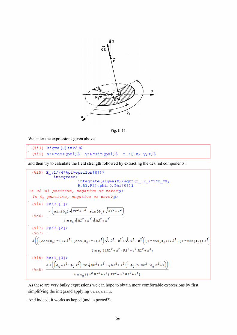
56

Fig. II.15

We enter the expressions given above

and then try to calculate the field strength followed by extracting the desired components:

As these are very bulky expressions we can hope to obtain more comfortable expressions by first

simplifying the integrand applying trigsimp.

And indeed, it works as hoped (and expected?).

57

In case of a full circle (0 = 2π) we get:

As one would expect only the z-component of the field is results as nonzero.

In case of an infinite plane (R1 = 0, R2 = ) we obtain:

So we received the well known result that the field strength is inverse proportional to the distance from the plane (see also problem II.10).

What will happen in case of a constant surface density?

58

As should be expected for the full circle of radius R2 (R1 = 0) we obtain %o12, which is the same as that obtained in the previous problem (II.14, expression %o4).

For the infinite plane we get the well known result (%o11) that field strength does not depend on the distance of the observed point from the plane.

■▬▬▬▬▬▬▬▬ II.16 A non-conductive rectangular plate of dimension a b lying in the xy-plane with its centre

in the origin is charged. The surface density depends on the position vector in the following

way: 0( ) 1 .y

yb

Find the vector of the electric field strength caused by this plate in a

generic point P(0,0,z0).

Solution:

Electric field strength in point P created by an element dx dy of the plate can be expressed according Coulomb's Law in the form

0 0 0 00 0

( ) ( )1 ( ) 1 ( )0 0 ,2 24 4( ) ( )

r r r rr rdE ds dx dy

r r r rr r r r

where 0 0( , , ), (0,0, )r x y z r z

denote the position vectors of the element of the plate dx dy and the

observed point, respectively.

Fig. II.16

The resultant vector of the electric field strength is obtained by integrating the above expression over the surface of the plate

/ 2 / 2 / 2 / 20 0

320 0 0 0/ 2 / 2 / 2 / 2 0

( ) ( )1 ( ) 1( ) .

4 ( ) 4

a b a b

a b a b

r r r rrE dy dx r dy dx

r r r r r r

59

The above integral seems to be too hard for wxMaxima, therefore we apply DERIVE.

We enter the data and the define the components:

The components are:

We can plot the components depending on z0 for special data:

■▬▬▬▬▬▬▬▬

60

II.17 An electric charge Q is distributed uniformly on a semi-sphere of radius R. Find the vector of the electric field in an arbitrary point on the axis of symmetry of the sphere.

Find the vector of the electric field in the centre of the sphere and in point B(0,0,-R).

Solution:

The contribution to the vector of the electric field dE

produced by an element dS of the semi-sphere is

given by

3 30 0

1 1 ,

4 4

dQ dSdE r r

r r

,

where denotes the surface charge density, 2

,2

Q

R

and at the observed point (0,0,z0) the vector r

is

0 0(0 ,0 , ) ( , , ).r r x y z z r x y z z

Fig. II.17

The resultant field vector is obtained by integrating the above expression over the whole semi-sphere

3 30 0

1 .

4 4S S

rE r dS dS

r r

If we use spherical coordinates

sin cos , sin sin , cos ,x R y R z R

then the surface element dS is given by: 2 sindS R d d

and the field vector in a point (0,0, 0z ) on the z axis can be written in the form:

/ 2 / 22 222

0 3 30 00 00 0

( ) sin sin .4 4

r R rE z R d d d d

r r

We enter the expression above and try to calculate the field vector (%06):

61

factor(E_) gives the simplest form of the result (cancelling z0):

To get the field in point B and in the centre we have to perform the respective substitutions (z0 = –R and z0 = 0):

Note: If we would like to calculate the field in the centre using result %o6 we need to apply the

limit command (see the error message as answer in %i11):

TI-NspireCAS has no problems performing the double integration:

62

II.18 A cylindrical dielectric layer characterized by two radii R1, R2 and height H is uniformly charged with a charge Q. Find the vector of the electric field

a) on the axis of symmetry,

b) in the centre of the base circle (see Fig. II.18).

Fig. II.18 Solution:

The contribution of an element dV of the hollow cylinder to the field vector dE

in point r

, is given

by

3 30 0

1 1,

4 4

dQdE r r dV

r r

where denotes the charge density 2 2

2 1

Q

R R H

.

The resultant field vector is the result of integrating dE

over the whole cylinder

0

3 30

1 .

4 4V V

rE r dV dV

r r

Due to the symmetry of the system, it is convenient to use cylindrical coordinates: According to Fig II.18 we can write

) , ,() ,0 ,0( 00 zzyxrzzyxrr

with

cos , sin , .x R y R dV R dR d dz

The resultant vector of the electric field is of the form

2

1

2

30

00

.4

H

R

R

rE R dR d dz

r

We enter the expressions given above:

63

a) At first we try to calculate the strength of the field using the trigsimp command within

the integration.

Graphic representation is obtained as follows.

b) In the point of interest (z0 = 0) the field takes a simpler form:

The many parameters invite introducing sliders for analyzing their influence on the strength of the field. We do this supported by TI-NspireCAS (we could also use DERIVE for this purpose). We can also ask for the position of the maximum strength.

64

Calculation is easy done. The screen below shows the graph from above (black) and the graph variable by moving the sliders (red). The maximum strength of the black graph is

given for z0 5.1 using the TI's Analyze-tool. It cannot be calculated exactly.

■▬▬▬▬▬▬▬▬

65

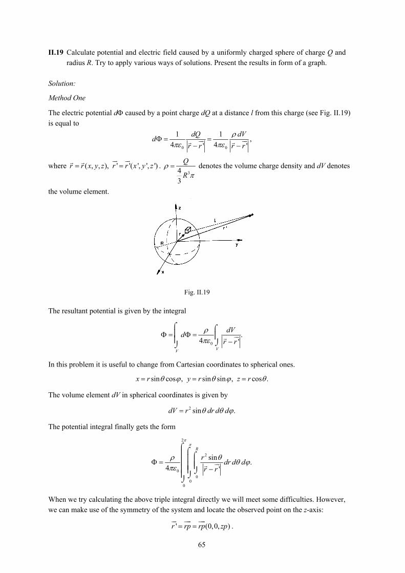
II.19 Calculate potential and electric field caused by a uniformly charged sphere of charge Q and radius R. Try to apply various ways of solutions. Present the results in form of a graph.

Solution:

Method One

The electric potential d caused by a point charge dQ at a distance l from this charge (see Fig. II.19)

is equal to

0 0

1 1,

4 4' '

dQ dVd

r r r r

where ( , , ), ' '( ', ', ')r r x y z r r x y z

. 34

3

Q

R

denotes the volume charge density and dV denotes

the volume element.

Fig. II.19 The resultant potential is given by the integral

0

.4 '

VV

dVd

r r

In this problem it is useful to change from Cartesian coordinates to spherical ones.

sin cos , sin sin , cos .x r y r z r

The volume element dV in spherical coordinates is given by

2 sin .dV r dr d d

The potential integral finally gets the form

2

2

00

00

sin.

4 '

R

rdr d d

r r

When we try calculating the above triple integral directly we will meet some difficulties. However, we can make use of the symmetry of the system and locate the observed point on the z-axis:

' (0,0, )r rp rp zp

.

66

Note: variable zp plays the role of the distance l of the observed point form the centre of the sphere.

We start the evaluation procedure:

We notice that Maxima is unable to perform the integration. Let's try to assist the program by stepwise integrating starting with the innermost integral:

Now we get a result for which can be further simplified:

The absolute value expression indicates that we have to distinguish between two cases:

R zp (observed point is inside the sphere) and R < zp (observed point is outside the sphere).

67

Thus we can enter the potential in form of a piecewise defined function (zp):

Field strength calculation uses the well known relation ( ).E grad

In our problem we need only

consider differentiation wrt zp.

Inside the sphere field strength increases proportional to the distance from the centre of the sphere

( zp), whereas outside it decreases inversely proportional to this distance 2

1.

zp

It is no problem to perform the integration with DERIVE:

68

But I came across problems working with TI-NspireCAS. I could perform the integration, but I could not obtain the "inside" result.

I wrote to Michel Beaudin (Canada) and he knew how to do overcome the problem. See Michel's answer and advice as well:

Josef, note that if the point is inside the sphere, we have R > zp.  So in order to compute the  value of 

« phi » in your Nspire file, yo need to split the integral into 2 parts because you don’t know if r is 

between 0 and zp or between zp and rr.  Doing this, Nspire gets the same results as good old Derive 

(see the file).   In Derive, we don’t need to do this because Derive is able to compute the whole 

integral because Derive is using a special rule of integration involving signum functions :  

int(f(x)*sign(a*x+b) = …….. 

Many thanks to Michel.

The plots are following on page 71.

69

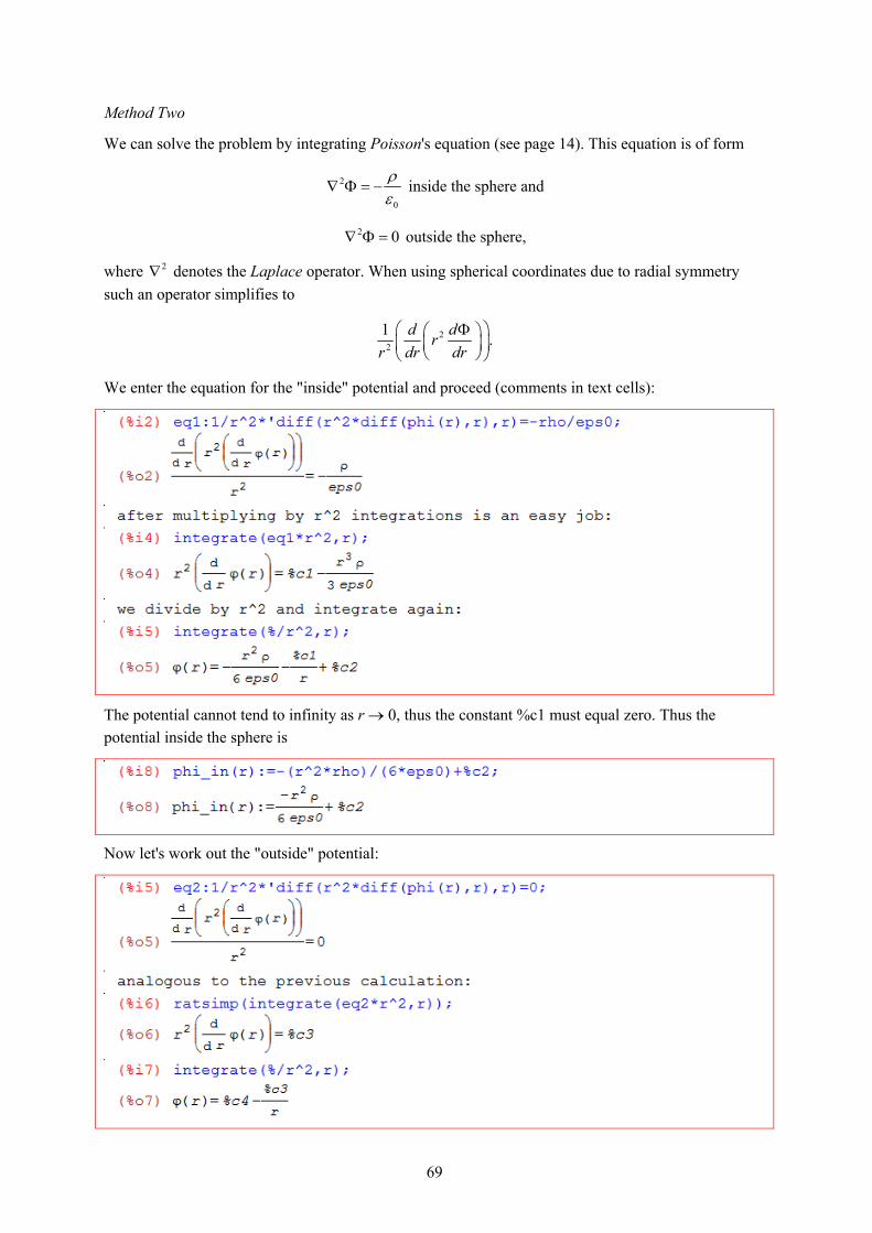
Method Two

We can solve the problem by integrating Poisson's equation (see page 14). This equation is of form

2

0

inside the sphere and

2 0 outside the sphere,

where 2 denotes the Laplace operator. When using spherical coordinates due to radial symmetry

such an operator simplifies to

22

1.

d dr

r dr dr

We enter the equation for the "inside" potential and proceed (comments in text cells):

The potential cannot tend to infinity as r 0, thus the constant %c1 must equal zero. Thus the

potential inside the sphere is

Now let's work out the "outside" potential:

70

It remains to determine the integration constants %c2 to %c4, from the boundary conditions:

the potential must tend to 0 for r and

potential and strength must be continuous on the surface of the sphere

which leads to the following three equations which can easily be solved:

We define the integration constants and bring the potential in its final concise form:

Finally we calculate the field strength:

71

Exercise: Substitute 34

3

Q

R

and check if results of Method 2 meet the results of Method 1.

We plot for Q = 1, eps0 = 1 and R = 2.

Potential (above) and Strength (below)

Method Three

The solution can be found in a much easier way using Gauss' law. This is left to the reader.

■▬▬▬▬▬▬▬▬

72

II.20 A solid dielectrical sphere with an empty spherical cavity is charged uniformly with volume

charge density . The centre of the spherical cavity is placed at a distance r0 from the centre

of the solid. Find the strength of the electric field at any point inside the cavity.

Fig. II.20

Solution: The spherical cavity can be treated as a uniformly charged sphere with zero volume charge

density, which can be modelled as a superposition of a positive density (+) and a negative density

(-) of equal magnitude. Then, by the superposition principle, the resultant electric field can be

calculated as the vector sum of the fields produced by the whole solid sphere of charge density

(+) and the sphere of charge density (- ) corresponding to the cavity.

From the solution of Problem II.16, we know that inside a uniformly charged solid sphere the electric field is given by

30

E r

.

According to Fig. II.20, we can write

1 2 1 2 00 0 0 0

.3 3 3 3

E R R R R r

■▬▬▬▬▬▬▬▬ II.21 We consider a system of two conducting balls of radii r1 and r2, separated by a large (in

comparison with the radii) distance d. How should a charge Q be distributed between the balls, if the force acting between the balls is to decrease after the balls have been connected by a thin wire?

Solution:

Since the distance between the balls is much larger than the sum of their radii, the balls can be treated as point charges. Therefore, the force acting between them is of the form

73

where Q1 is the charge on the ball of radius r1 and (Q – Q1) the charge on the other ball. After the balls have been connected by a thin wire, the charge is redistributed and the new force is

where q1 and (Q – q1) are new charges.

When the balls are connected by a wire, then the potential difference disappears (the potentials on the balls are the same). Using the expression for the potential on a metallic ball of radius r charged with a charge q

one can write the equation

1 1 1 2( , ) ( , ).q r Q q r

Charge q1 is the solution of the above equation:

In order to find Q1 we have to solve the following inequality

F1 < F i.e. F1 – F < 0.

It can easily be seen that the above inequality is true within the zeros of a second order polynomial (parabola). Let's find these zeros now.

From %o7 we can conclude that for r2 < r1 the solution is

2 11

1 2 1 2

Q r Q rQ

r r r r

and consequently when r2 > r1 then we have

1 21

1 2 1 2

.Q r Q r

Qr r r r

The screen shots on the next page demonstrate that DERIVE and TI-NspireCAS as well can solve the inequality F1 – F < 0.

74

The solution of TI-NspireCAS is a "little bit" bulky and includes a lot of additional information. It should not be really funny to read this solution on a handheld.

■▬▬▬▬▬▬▬▬ II.22 The sketch shows two point charges Q and 2Q. Ql charge is uniformly distributed on the

segment of length l.

Fig. II.22

Find the angel and relationship of Ql/Q charges for which the Coulomb force is

disappearing in the centre of the coordinate system.

Solution:

Coulomb force is zero implies the electric field to be zero. Therefore it remains to inspect the electric field. The resultant field is a vector sum of the fields created by the point charges and the Ql charge. For the point charges we have

75

and for the charge Ql we will write

Then the resultant field is the sum and will be evaluated applying the requested relationship of the

charges Ql = Q ( is the factor of proportionality).

We try to find the desired parameters and in one single step.

(Remember, the solve function doesn't need the right hand side of the equation when it equals zero.)

As this does not work we will try to find the solution step by step (good old elimination method). From the first equation we get

We know that trig equations in most cases have more solutions – let's try later with another CAS.

Now we will proceed finding .

Finally we are verifying the correctness of the obtained solution.

76

We will tackle this problem with TI-NspireCAS and DERIVE as well. TI-NspireCAS allows solving the system of equations in one step but the output is again more than bulky so that it might not be comfortable to read it off from the handheld. At the other hand TI-NspireCAS gives more than one solution.

So does DERIVE. Calculation procedure is not complicated and the output is very handsome, isn't it.