cascade sliding mode control of a field oriented induction motors...
TRANSCRIPT

1. Introduction
The induction machine is widely used in industry, because of its mechanical robustness, lowmaintenance requirement, and relatively low cost. However, from control point of view,control of the induction machines is one of the most challenging topics. Its control is complexbecause the dynamic of the induction machine is nonlinear, multivariable, and highly coupled.Furthermore, there are various parameter uncertainties and disturbances in the system. Therotor resistances, for example, can vary up to 100% because of rotor heating during operation.In the last few years, many versions of a nonlinear state feedback control schemes, such as,input-output feedback linearization ((Marino et al., 1993)), passivity-based control ((Ortega& Espinoza, 1993; Ortega et al., 1996)) and Backstepping (Kanellakopoulos et al. (1991);Krstic et al. (1995)) have been applied to the IM drive. Adaptive versions of most of thosenonlinear control schemes are also available for the effective compensation of the parameteruncertainties and disturbances in the induction motor systems (Ebrahim & Murphy (2006);Marino et al. (1993); Ortega et al. (1993); Rashed et al. (2006)). A fundamental problem inthe design of feedback controllers is that of stabilizing and achieving a specified transientperformance in the presence of external disturbances and plant parameter variations.Since the publication of the survey paper by (Utkin (1977)), significant interest on Slidingmode control has been generated in the control research community worldwide. Thisinterest is increased in the last two decades due to the possibility to implement this controlin industrial applications with the advances of the power electronics technology and theavailability of cheap and fast computation.One of the most intriguing aspects of sliding mode is the discontinuous nature of the controlaction whose primary function of each of the feedback channels is to switch between twodistinctively different system structures (or components) such that a new type of systemmotion, called sliding mode, exists in a manifold. This peculiar system characteristic isclaimed to result in superior system performance which includes insensitivity to parametervariations, and complete rejection of disturbances (Young et al. (1999)).In this paper, a nonlinear adaptive Sliding mode speed and rotor flux control schemecombined with field orientation for the induction-motor drive has been developed. Somesliding surfaces are chosen for which an appropriate logic commutation associated to thesesurfaces is determined. One important characteristic of the proposed controller is its cascadestructure; witch gives a high performance using simple sliding surfaces. Furthermore, in orderto reduce chattering phenomenon, smooth control functions with appropriate threshold have
Abdellatif REAMA, Fateh MEHAZZEM and Arben CELAESIEE Paris- Paris Est University
France
Cascade Sliding Mode Control of a Field Oriented Induction Motors
with Varying Parameters
8
www.intechopen.com

been chosen. The rotor flux is estimated using the rotor-circuit model and, thus, is insensitiveto the stator resistance. A stable model reference adaptive system (MRAS) rotor-resistanceand load torque estimators have been designed using the measured stator current and rotorspeed, and voltage command.
2. Indirect field-oriented control of the IM
Assuming linear magnetic circuits and balanced three phase windings, the fifth-ordernonlinear model of IM (Krauss (1995)), expressed in the stator frame is :
dω
dt=
3npLm
2JL2(λ2ai1b − λ2bi1a) −
TL
J
dλ2a
dt= −
R2
L2λ2a − npωλ2b +
R2
L2Lmi1a
dλ2b
dt= −
R2
L2λ2b + npωλ2a +
R2
L2Lmi1b (1)
di1a
dt=
LmR2
σL1L22
λ2a +npLm
σL1L2ωλ2b −
L2mR2 + L2
2R1
σL1L22
i1a+1
σL1u1a
di1b
dt=
LmR2
σL1L22
λ2b −npLm
σL1L2ωλ2a −
L2mR2 + L2
2R1
σL1L22
i1b+1
σL1u1b
We can see that the model described by (1) is highly coupled, multivariable and nonlinearsystem. It is very difficult to control the IM directly based on this model. State transformationto simplify the system representation is required. A well-known method to this end isthe transformation of the field orientation principle. It involves basically a change ofthe representations of the state vector (i1a, i1b, λ2a, λ2b) in the fixed stator frame (a, b) intoa new state vector in a frame (d, q) which rotates along with the flux vector (λ2a, λ2b).Mathematically, the field oriented transformation can be described as:
i1d =λ2ai1a + λ2bi1b√
λ22a + λ2
2b
, i1q =λ2ai1b − λ2bi1a√
λ22a + λ2
2b
(2)
λ2d =√
λ22a + λ2
2b, λ2q = 0, ρ = arctan
(
λ2b
λ2a
)
Where much simplification is gained by the fact that λ2q = 0 . Using this transformation andthe notations in the Nomenclature, the state equations (1) can be rewritten in the new statevariables as:
dw
dt= μλ2di1q −
TL
J
di1q
dt= −η1i1q − βnpωλ2d − npωi1d − R2(η2i1q+αLm
i1qi1d
λ2d) +
1
σL1u1q
λ2d
dt= −αR2λ2d + αLmR2i1d
156 Sliding Mode Control
www.intechopen.com
di1d
dt= −η1i1d + npωi1q + R2(−η2i1d + αβλ2d + αLm
i21q
λ2d)+
1
σL1u1d (3)
dρ
dt= npω + αLmR2
i1q
λ2d
The decoupling control method with compensation is to choose inverter output voltages suchthat:
u∗
1d =
(
Kp + Ki1
s
)
(i∗1d − i1d) − ρL1σi∗1q + L1σdi∗1q
dt
u∗
1q =
(
Kp + Ki1
s
)
(
i∗1q − i1q
)
+ ρL1σi∗1d + ρLm
L2λ2d (4)
Where Kp, Ki are PI controller gains.For that, we need the estimation of the rotor flux as given by
˙λ2d = −αR2λ2d + αLmR2i1d (5)
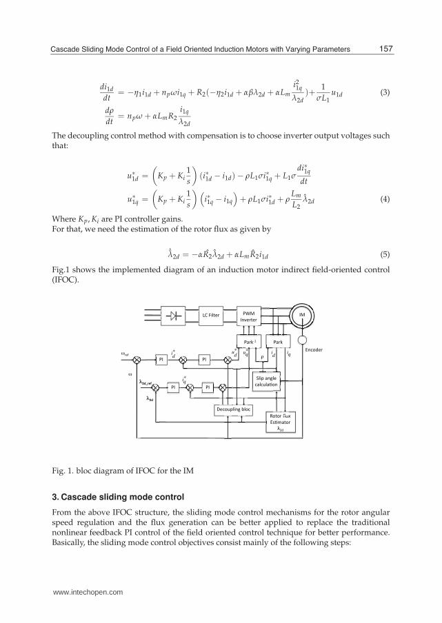
Fig.1 shows the implemented diagram of an induction motor indirect field-oriented control(IFOC).
%' &! $46=0; (+' %8A0;=0;
(,;5 (,;5EF
*64: ,8360 .,6.@6,>98
)9=9; 2@B #<>7,=9;
DG/
"0.9@:6483 -69.
8
(% (%
(% (%
2@B6483 -693
#8.9/0; ρ
ud
* uq* i
diqω;01
ω
λλ&!%$"#
λ&!
id
*
iq*
Fig. 1. bloc diagram of IFOC for the IM
3. Cascade sliding mode control
From the above IFOC structure, the sliding mode control mechanisms for the rotor angularspeed regulation and the flux generation can be better applied to replace the traditionalnonlinear feedback PI control of the field oriented control technique for better performance.Basically, the sliding mode control objectives consist mainly of the following steps:
157Cascade Sliding Mode Control of a Field Oriented Induction Motors with Varying Parameters
www.intechopen.com

3.1 Design of the switching surfaces
We choose the sliding surface to obtain a sliding mode regime which guarantees theconvergence of the state x to its desired value xd according to the relation (6) (Slotine & Li(1991):
S(x) =
(
d
dt+ λ
)r−1
e (6)
Where e = xd − x: tracking errorλ: positive coefficientr: relative degreeSuch in IFOC structure, we have four PI controllers; we will define four sliding surfaces(Mahmoudi et al. (1999)):
S1 (ω) = ωre f − ω
S2 (λ2d) = λ2dre f − λ2d
S3
(
i1q
)
= i∗1q − i1q (7)
S4 (i1d) = i∗1d − i1d
3.2 Control calculation
Two parts have to be distinguished in the control design procedure. The first one concerns theattractivity of the state trajectory to the sliding surface and the second represents the dynamicresponse of the representative point in sliding mode. This latter is very important in termsof application of nonlinear control techniques, because it eliminates the uncertain effect of themodel and external perturbation. For that, the structure of a sliding mode controller includestwo terms:
uc = ueq + un (8)
Where-ueq is called equivalent control which is used when the system state is in the sliding mode. It
is calculated from S (x) = 0.-un is given to guarantee the attractivity of the variable to be controlled towards thecommutation surface. This latter is achieved by the condition (Slotine & Li (1991); Utkin(1993)).
S (x) .S (x) < 0 (9)
A simple form of the control action using sliding mode theory is a relay function; witch has adiscontinuous form given by:
un = −k.sgn (S (x)) (10)
k is a constant and is chosen positive to satisfy attractivity and stability conditions.
158 Sliding Mode Control
www.intechopen.com

3.2.1 For the rotor flux regulation
S2 (λ2d) = 0 ⇒ i1deq =λ2d + Trλ2dre f
Lm(11)
S2 (λ2d) S2 (λ2d) < 0 ⇒ i1dn = Kφ.sign (S2 (λ2d)) (12)
Thus the controller is
i1dc = i1deq + i1dn (13)
3.2.2 For the direct current regulation
S4 (i1d) = 0 ⇒
u1deq = σL1 i1dre f + Rsmi1d − σL1ωsi1q −Lm
L2Trλ2d
(14)
S4 (i1d) S4 (i1d) < 0 ⇒ u1dn = Kd.sign (S4 (i1d)) (15)
The controller is given by
u1dc = u1deq + u1dn (16)
3.2.3 For the speed regulation
S1 (ω) = 0 ⇒ i1qeq =Jωre f + Fω + TL
pLm
L2λ2d
(17)
S1 (ω) S1 (ω) < 0 ⇒ i1qn = Kω .sign (S1 (ω)) (18)
The controller is given by
i1qc = i1qeq + i1qn (19)
3.2.4 For the quadrature current regulation
S3
(
i1q
)
= 0 ⇒
u1qeq = σL1 i1qre f + Rsmi1q + σL1ωsi1d +Lm
L2ωλ2d
(20)
S3
(
i1q
)
S3
(
i1q
)
< 0 ⇒ u1qn = Kq.sign(
S3
(
i1q
))
(21)
The controller is given by
u1qc = u1qeq + u1qn (22)
To satisfy stability condition of the system, all of the following gains (Kd, Kq, Kφ, Kω) shouldbe chosen positive.
159Cascade Sliding Mode Control of a Field Oriented Induction Motors with Varying Parameters
www.intechopen.com

4. Load torque estimator
Since the load torque is not exactly known, its estimation is introduced. The mechanicalequation gives
TL =pLm
L2λ2di1q − J
dω
dt− Fω (23)
5. Mras rotor resistance identification
As the estimated rotor flux is sensitive to rotor-resistance variation, a stable rotor-resistanceMRAS estimator can be developed. We can rewrite the dynamic model of an inductionmotor given before by equations (11) as a compact form given by (Leonhard (1984); Pavlov& Zaremba (2001)) :
dw
dt=
3
2
npLm
JL2iT1 Mλ2 −
TL
J(24)
dλ2
dt=
(
−R2
L2I + npwM
)
λ2 +R2
L2Ji1 (25)
di1dt
= −J
σL1L2
(
−R2
L2I + npwM
)
λ2 −1
σL1
(
R1 +J2R2
L22
)
i1 +1
σL1u1 (26)
Where
I =
(
1 00 1
)
, M =
(
0 −11 0
)
In order to design a rotor resistance identifier equations (25) (26) are transformed to eliminatethe unobservable rotor flux. At this point an assumption is made that the rotor speed changessignificantly slower relative to the rotor flux. Thus it may be treated as a constant parameter.First differentiating (26) and eliminating λ2 gives
d2i1dt2
= (α1 I + wβ1 M)di1dt
+ (α2 I + wβ2 M) i1 + (α3 I + wβ3 M) u1 + α4du1
dt(27)
where
α1 = −1
σL1
(
R1 +L2
mR2
L22
)
−R2
L2, β1 = np,
α2 = −R2R1
σL2L1, β2 =
npR1
σL1,
α3 =R2
σL1L2, β3 = −
np
σL1, α4 =
1
σL1.
Adding cdi1/dt, c > 0, to both sides of (27) and formally dividing by (d/dt + c) transforms(27) to
di1dt
= a + ωb + ǫ (28)
160 Sliding Mode Control
www.intechopen.com
where ǫ → 0 exponentially and the functions a and b are linear combinations of the filteredstator current and stator voltage command:
a = (c + α1) i11 + α2i10 + α3u10 + α4u11
b = M (β1i11 + β2i10 + β3u10)
where
i10 =1
s + ci1, i11 =
s
s + ci1
u10 =1
s + cu1, u11 =
s
s + cu1 (29)
Here s denotes d/dt.To obtain a reference model for the rotor resistance identification the part of the right-handside of (28) containing R2 is separated:
di1dt
= f1 + R2 f2 + ωM f3 + ǫ (30)
where
f1 = (c + ρ1) i11 + ρ2u11
f2 = γ1i11 + γ2i10 + γ3u10 (31)
f3 = β1i11 + β2i10 + β3u10
Coefficients in (31) are calculated according to the following formulae:
ρ1 = −R1
σL1, ρ2 =
1
σL1,
β1 = np, β2 =npR1
σL1, β3 = −
np
σL1,
γ1 = −1
L2
(
1 +L2
m
σL1L2
)
, γ2 =ρ1
L2, γ3 =
ρ2
L2.
Since ω is available for measurement the design of an R2 identifier is straightforward. Itis based on the MRAS identification approach (Sastry & Bodson (1989)) with(30) being areference model.Within this approach an identifier consists of a tuning model depending on an estimate of theunknown parameter and a mechanism to adjust the estimate. This adjustment is performedto make the output of the tuning model asymptotically match the output of the referencemodel. In our case the tuning model is given by
di1dt
= −L(
i1 − i1)
+ f1 + ωM f3 + R2 f2 (32)
where L > 0 is a constant and R2 is the estimate of R2. The dynamics of the error e = i1 − i1 isthe following
de
dt= −Le +
(
R2 − R2
)
f2 − ǫ (33)
161Cascade Sliding Mode Control of a Field Oriented Induction Motors with Varying Parameters
www.intechopen.com
The adjustment equation for R2 is
dR2
dt= −γ
(
i1 − i1)T
f2, γ > 0. (34)
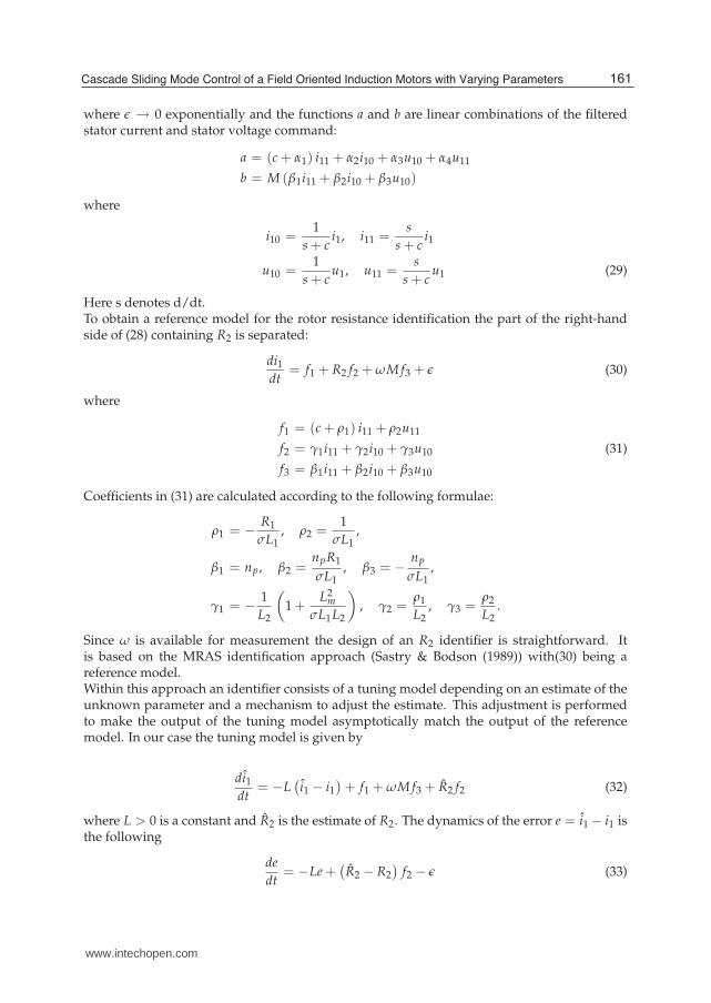
Fig. 2. Overall bloc diagram of the control scheme for IM
6. Simulations results
The overall configuration of the control system for IM is shown in Fig.2. The effectivenessof the proposed controller combined with the rotor resistance and load torque estimationshas been verified by simulations in Matlab/Simulink. The parameters of the induction motorused are given in Appendix. The simulation results have been obtained under a constant loadtorque of 10 Nm.Parameters of the Sliding mode controllers are: Kd = 500, Kq = 500, Kφ = 400 and Kω = 300.Parameters of the MRAS identifier are: γ = 0.2, L = 100 and c = 0.01.Results obtained are shown in Fig.3. The reference speed is set to 200 rad/s until t=4s, when itis reversed to -200rad/s to allow drive to operate in the generating mode. The reference fluxis set to 0.4wb. The load torque is changed from 0 to 10 Nm at t=0.6s. The rotor resistanceand the load torque estimators are activated. It can be seen that the estimated load torqueconverges very quickly to the actual value. In addition, the estimated values of R2 follow itsactual value very closely.In order to show the convergence capability of the MRAS rotor resistance estimator, at t=1.2s, the interne value of R2 in the MAS model has been disturbed and varied intentionally 30%
!
"#
$
#%
&
!
'(
"#)(
!
!
*
'
!
!
ˆ
162 Sliding Mode Control
www.intechopen.com

of its initial value and held constant until t=2.5s, at the same moment, the rotor resistanceestimator is disconnected from the control structure.It can be noted that the error in the estimated value of R2 produces a steady state error in thespeed and the rotor flux control and also generates an error in the estimated value of the loadtorque.At t=2.5s, the initial value of R2 in MAS model has restored and the rotor resistance estimatorhas been reconnected and the rotor resistance is seen to converge to the actual value and alsothe other system variables.At t=4s, the reference speed is reversed to -200 rad/s to allow the drive to operate in thegenerating mode.The results show a stable operation of the drive in the various operating modes.
0 1 2 3 4 5 6 7-250
-200
-150
-100
-50
0
50
100
150
200
250
0 1 2 3 4 5 6 70
0.1
0.2
0.3
0.4
0.5
0.6
0.7
0 1 2 3 4 5 6 7-2
0
2
4
6
8
10
12
0 1 2 3 4 5 6 71.1
1.2
1.3
1.4
1.5
1.6
1.7
1.8
1.9
Time (s)
R2
_es
t, R
2(o
hm
s)
T
l_es
t, T
l(N
.m)
F
lux (
wb
)
S
pee
d (
rad/s
)
d
ref_d
2
2
λ
λ
ω
ωref
L
L
T
T
2
2
R
R
(a)
(b)
(d)
(c)
Fig. 3. Tracking Performance and parameters estimates : a)reference and actual motorspeeds, b)reference and actual rotor flux, c)TL and TL(N.m), d)R2 and R2(Ω).
163Cascade Sliding Mode Control of a Field Oriented Induction Motors with Varying Parameters
www.intechopen.com

Furthermore, simulation results have been performed to show the capability of the load torqueestimator to track the rapid load torque changes and also to show the performance of flux andspeed control. The results are shown in Fig. 4. These results have been obtained using thesame parameters used for the results in Fig. 3. The rotor resistance and load torque estimatorsare activated at t=0.2s. The load torque has been reversed from 10 Nm to -10 Nm at t=2s. Itcan be seen from Fig. 4 that the estimated load torque converges rapidly to its actual valueand the rotor resistance estimator is stable. In addition, the results in Fig. 4 show an excellentcontrol of rotor flux and speed.
Time (s)
R2
_es
t, R
2(o
hm
s)
Tl_
est
, T
l(N
.m)
F
lux (
wb)
Sp
eed (
rad/s
)
0 1 2 3 4 5 6 7-250
-200
-150
-100
-50
0
50
100
150
200
250
0 1 2 3 4 5 6 70
0.1
0.2
0.3
0.4
0.5
0.6
0.7
0 1 2 3 4 5 6 7-15
-10
-5
0
5
10
15
0 1 2 3 4 5 6 71.2
1.21
1.22
1.23
1.24
1.25
1.26
1.27
1.28
ω
ωref
d
ref_d
2
2
λ
λ
L
L
T
T
2
2
R
R
(a)
(b)
(c)
(d)
Fig. 4. Tracking Performance and parameters estimates : a)reference and actual motorspeeds, b)reference and actual rotor flux, c)TL and TL(N.m), d)R2 and R2(Ω).
Thus, the simulation results confirm the robustness of the proposed scheme with respect tothe variation of the rotor resistance and load torque.
164 Sliding Mode Control
www.intechopen.com

7. Conclusions and future works
In this paper, a novel scheme for speed and flux control of induction motor using onlineestimations of the rotor resistance and load torque have been described. The nonlinearcontroller presented provides voltage inputs on the basis of rotor speed and stator currentsmeasurements and guarantees rapid tracking of smooth speed and rotor flux references forunknown parameters (rotor resistance and load torque) and non-measurable state variables(rotor flux). In simulation results, we have shown that the proposed nonlinear adaptivecontrol algorithm achieved very good tracking performance within a wide range of theoperation of the IM. The proposed method also presented a very interesting robustnessproperties with respect to the extreme variation of the rotor resistance and reversal of theload torque. The other interesting feature of the proposed method is that it is simple and easyto implement in real time.From a practical point of view, in order to reduce the chattering phenomenon due to thediscontinuous part of the controller, the sign(.) functions have been replaced by the saturation
functions(.)
(. )+0.01(Slotine & Li (1991).
It would be meaningful in the future work to implement in real time the proposed algorithmin order to verify its robustness with respect to the discretization effects, parameteruncertainties and modelling inaccuracies.
Induction motor dataStator resistance 1.34 Ω
Rotor resistance 1.24 Ω
Mutual inductance 0.17 HRotor inductance 0.18 HStator inductance 0.18 HNumber of pole pairs 2 H
Motor load inertia 0.0153 Kgm2
NomenclatureR1, R2 rotor, stator resistancei1, i2 rotor, stator currentλ1, λ2 rotor, stator flux linkageλ2d amlpitude of rotor flux linkageu1, u2 rotor, stator voltage inputω rotor angular speedωs stator angular frequencyρ rotor flux anglenp number of pole pairsL1, L2 rotor, stator inductanceTr rotor time constantLm mutual inductanceJ, TL inercia, load torqueF coefficient of friction(.)d, (.)q in (d,q) frame(.)a, (.)b in (a,b) frame(.) estimate of (.)(.∗) reference of (.)
165Cascade Sliding Mode Control of a Field Oriented Induction Motors with Varying Parameters
www.intechopen.com

σ = 1 −L2
m
L1L2, α =
1
L2, β =
Lm
σL1L2, η1 =
R1
σL1
η2 =L2
m
σL1L22
, μ =3npLm
2JL2, Rsm = R1 +
L2m
L22
R2
8. References
Ebrahim, A. & Murphy, G. (2006). Adaptive backstepping control of an induction motor undertime-varying load torque and rotor resistance uncertainty, Proceedings of the 38thSoutheastern Symposium on System Theory Tennessee Technological University Cookeville .
Kanellakopoulos, I., Kokotovic, P. V. & Morse, A. S. (1991). Systematic design ofadaptive controllers for feedback linearizable systems, IEEE Trans. Automatic Control36: 1241–1253.
Krauss, P. C. (1995). Analysis of electric machinery, IEEE Press 7(3): 212–222.Krstic, M., Kannellakopoulos, I. & Kokotovic, P. (1995). Nonlinear and adaptive control
design, Wiley and Sons Inc., New York pp. 1241–1253.Leonhard, W. (1984). Control of electric drives, Springer Verlag .Mahmoudi, M., Madani, N., Benkhoris, M. & Boudjema, F. (1999). Cascade sliding mode
control of field oriented induction machine drive, The European Physical Journalpp. 217–225.
Marino, R., Peresada, S. & Valigi, P. (1993). Adaptive input-output linearizing control ofinduction motors, IEEE Transactions on Automatic Control 38(2): 208–221.
Ortega, R., Canudas, C. & Seleme, S. (1993). Nonlinear control of induction motors:Torque traking with unknown disturbance, IEEE Transaction On Automatic Control38: 1675–1680.
Ortega, R. & Espinoza, G. (1993). Torque regulation of induction motor, Automatica29: 621–633.
Ortega, R., Nicklasson, P. & Perez, G. E. (1996). On speed control of induction motor,Automatica 32(3): 455–460.
Pavlov, A. & Zaremba, A. (2001). Real-time rotor and stator resistances estimation of aninduction motor, Proceedings of NOLCOS-01, St-Petersbourg .
Rashed, M., MacConnell, P. & Stronach, A. (2006). Nonlinear adaptive state-feedbackspeed control of a voltage-fed induction motor with varying parameters, IEEETRANSACTIONS ON INDUSTRY APPLICATIONS 42(3): 1241–1253.
Sastry, S. & Bodson, M. (1989). Adaptive control: stability, c onvergence, and robustness,Prentice Hall. New Jersey .
Slotine, J. J. & Li, W. (1991). Applied nonlinear control, Prentice Hall. New York .Utkin, V. (1993). Sliding mode control design principles and applications to electric drives,
IEEE Transactions On Industrial Electronics 40: 26–36.Utkin, V. I. (1977). Variable structure systems with sliding modes, IEEE Transaction on
Automatic Control AC-22: 212–222.Young, K. D., Utkin, V. I. & Ozguner, U. (1999). A control engineer’s guide to sliding mode
control, IEEE Transaction on Control Systems Technology 7(3): 212–222.
166 Sliding Mode Control
www.intechopen.com

Sliding Mode ControlEdited by Prof. Andrzej Bartoszewicz
ISBN 978-953-307-162-6Hard cover, 544 pagesPublisher InTechPublished online 11, April, 2011Published in print edition April, 2011
InTech EuropeUniversity Campus STeP Ri Slavka Krautzeka 83/A 51000 Rijeka, Croatia Phone: +385 (51) 770 447 Fax: +385 (51) 686 166www.intechopen.com
InTech ChinaUnit 405, Office Block, Hotel Equatorial Shanghai No.65, Yan An Road (West), Shanghai, 200040, China
Phone: +86-21-62489820 Fax: +86-21-62489821
The main objective of this monograph is to present a broad range of well worked out, recent applicationstudies as well as theoretical contributions in the field of sliding mode control system analysis and design. Thecontributions presented here include new theoretical developments as well as successful applications ofvariable structure controllers primarily in the field of power electronics, electric drives and motion steeringsystems. They enrich the current state of the art, and motivate and encourage new ideas and solutions in thesliding mode control area.
How to referenceIn order to correctly reference this scholarly work, feel free to copy and paste the following:
Abdellatif Reama, Fateh Mehazzem and Arben Cela (2011). Cascade Sliding Mode Control of a Field OrientedInduction Motors with Varying Parameters, Sliding Mode Control, Prof. Andrzej Bartoszewicz (Ed.), ISBN: 978-953-307-162-6, InTech, Available from: http://www.intechopen.com/books/sliding-mode-control/cascade-sliding-mode-control-of-a-field-oriented-induction-motors-with-varying-parameters